


1. Introduction
Natural convection induced by internal heat production is a phenomenon that occurs very often in geophysical, astrophysical and engineering systems (Goluskin Reference Goluskin2015). By following the analysis recently given by Creyssels (Reference Creyssels2020), the purpose of this paper is to extend the many theoretical, numerical and experimental results of Rayleigh–Bénard (RB) convection to two internally heated (IH) convection systems shown in figures 1(a) and 1(b). In RB convection, convective flow is produced by thermal boundary conditions that cause heat to enter through the lower hot plate and exit through the upper cold plate. In this case, convection is controlled by the temperature difference between the plates ( ${\rm \Delta} T$) and the height of the cell (
 $h$), or by the Rayleigh number defined as
 \begin{equation} Ra = \frac{g \beta {\rm \Delta} T h^3}{\nu \kappa}, \end{equation}
where  $g$ is the uniform gravitational acceleration,
  $\beta$,
  $\nu$ and
  $\kappa$ are, respectively, the coefficient of thermal expansion, the kinematic viscosity and the thermal diffusivity of the fluid. On the contrary, for IH convection, the flow is produced by a volumetric source of internal heating (
 $q$ in W m
 $^{-3}$), itself produced by chemical or nuclear reactions, or by radiation. Instead of using
  $Ra$, the Rayleigh–Roberts number (Roberts Reference Roberts1967) is adopted as follows
 \begin{equation} Rr = \frac{g \beta q h^5}{\lambda \nu \kappa}, \end{equation}
where  $\lambda$ is the thermal conductivity of the fluid. A first approach of IH convection is to take
  $q$ constant and uniform throughout the volume. Using
  $h^2 / \kappa$ as the unit of time,
  $h$ as the unit of length and
  $q h^2/ \lambda$ as the unit of temperature, the dimensionless Boussinesq equations governing the velocity
  $(\tilde{\boldsymbol{u}})$, pressure
  $(\tilde{p})$ and temperature
  $(\tilde{T})$ are the incompressibility condition (
 $\boldsymbol {\nabla }\boldsymbol {\cdot }\boldsymbol {u}$) and
 $$\begin{gather} \widetilde{\partial_t} \tilde{\boldsymbol{u}} + \tilde{\boldsymbol{u}} \boldsymbol{\cdot} \widetilde{\boldsymbol{\nabla}} \tilde{\boldsymbol{u}} ={-} \widetilde{\boldsymbol{\nabla}} \tilde{p} + Pr \widetilde{\nabla}^2 \tilde{\boldsymbol{u}} + Pr \, Rr \, \tilde{T} \, \boldsymbol{\hat{e}}_z, \end{gather}$$
 $$\begin{gather}\widetilde{\partial_t} \tilde{T} + \tilde{\boldsymbol{u}} \boldsymbol{\cdot} \widetilde{\boldsymbol{\nabla}} \tilde{T} = \widetilde{\nabla}^2 \tilde{T} + 1, \end{gather}$$
where dimensionless variables and operators are designated by tildes,  $\boldsymbol {\hat {e}}_z$ is the vertical unit vector and
  $Pr$ is the Prandtl number. With regard to thermal boundary conditions, we consider hereafter those used by most of previous studies i.e. fixed and equal temperature conditions (
 $T_0$) at the top and bottom plates. By adopting this condition, modelling an IH convection experiment becomes a great challenge because in a single cell, there are both positive and negative vertical mean temperature gradients (see figure 1b). This leads to both turbulent convection and a stably stratified lower boundary layer. Therefore, the experiments on RB and IH convection have some similarities but also some differences. For both cases, the mean temperature is almost constant in the middle of the cell and we call it the temperature of the ‘bulk flow’ (
 $\bar {T}_b$). At high
  $Ra$ numbers and assuming negligible non-Boussinesq effects,
  $\bar {T}_b$ is equal to the average of the top and bottom plate temperatures for a RB experiment, while
  $\bar {T}_b$ is the maximum of the mean temperature in an IH convection cell (see figure 1b). Besides, the two thermal boundary layers located near the top and bottom plates have the same thickness for a RB experiment. On the contrary, heating in volume leads to an asymmetry between the two thermal boundary layers. The mean temperature profile was measured by Goluskin & van der Poel (Reference Goluskin and van der Poel2016) and is shown in figure 1(b). Therefore, the upper boundary layer is similar to that observed in a RB experiment, whereas in the lower boundary layer, the mean temperature gradient tends to stop convective flows produced in the upper region of the cell. Consequently, in an IH convection cell, the thickness of the lower boundary layer is greater than that of the upper boundary layer (
 $\delta _{bot} > \delta _{top}$). In addition, the difference in thickness must increase as the Rayleigh number increases. Likewise, at a fixed
  $Ra$ number, the mean vertical heat flux is constant for a RB experiment and is given by the Nusselt number as
  $\varPhi _{RB} = Nu_{RB} ({\lambda {\rm \Delta} T}/{h})$. In contrast, in an IH convection cell, the heat produced inside the fluid is evacuated through both lower and upper boundaries, leading to a mean vertical heat flux that changes sign from the bottom plate to the top plate (see figure 1b). As the mechanisms that drive the two thermal boundary layers are different, the heat fluxes through the upper and lower plates are not equal in absolute value. A coefficient
  $\alpha$ can be defined to quantify this down–up asymmetry. Indeed, the fraction of heat produced inside the fluid flowing outwards from the bottom plate can be written as
 \begin{equation} q_{bot} = \left(\tfrac{1}{2}-\alpha\right) q, \end{equation}
leading to a heat flux at the bottom plate equal to  $- q_{bot} h \boldsymbol {e}_z$. In steady state, energy conservation yields to a heat flux that leaves through the top plate as
  $q_{top} h \boldsymbol {e}_z$, with
 \begin{equation} q_{top} = \left(\tfrac{1}{2}+\alpha\right) q. \end{equation}
Then, for each plate, we can define one Nusselt number as
 $$\begin{gather} Nu_{bot} = \frac{q_{bot} h^2}{\lambda {\rm \Delta} T}, \end{gather}$$
 $$\begin{gather}Nu_{top} = \frac{q_{top} h^2}{\lambda {\rm \Delta} T}. \end{gather}$$
To be consistent with the definition of the Nusselt number adopted for RB convection experiments, the characteristic temperature difference  ${\rm \Delta} T$ used in (1.7) and (1.8) is
  ${\rm \Delta} T = 2 (\bar {T}_b - T_0)$. There is therefore a factor 2 by comparing the definitions of
  $Nu_{bot}$ and
  $Nu_{top}$ given in previous studies on IH convection (Goluskin Reference Goluskin2015). Note also that other definitions of Nusselt numbers are given in the literature. Instead of using
  $\bar {T}_b$, the mean fluid temperature (
 $\langle \bar {T} \rangle$, where angle brackets denote an average over the entire volume) can be chosen as temperature reference in (1.7) and (1.8). Figure 6(a) shows that the difference of temperature
  $\bar {T}_b - \langle \bar {T} \rangle$ becomes negligible only for very high Rayleigh–Roberts numbers.

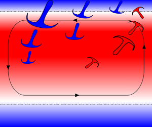
Figure 1. Two convective systems are theoretically studied here. Configuration (a) is closer to standard RB experiments since the two hot and cold plates play the same role and the same heat flux ( $\varPhi _0$) crosses them. But the heat flux at the centre of the cell is lower or greater than
  $\varPhi _0$, depending on the sign of
  $q$:
$q$:  $\bar {\varPhi }_a(z\!=\!h/2) = {\varPhi }_0-qh/2$. Configuration (b) is more complex because the upper half-cell is very similar to the upper half-cell of RB experiments whereas the flow is stratified in the lower part of the bottom half-cell. The heat flux at the bottom plate is negative (
 $-q_{bot}h$) and is not equal in absolute value to the heat flux at the top plate (
 $q_{top}h$). Besides,
  $q_{top}>q_{bot}$. For configuration (b), the mean temperature profile
  $\bar {T}(z)$ was measured by Goluskin & van der Poel (Reference Goluskin and van der Poel2016). The upper and lower thermal boundary layers of thickness
  $\delta _{top}$ and
  $\delta _{bot}$ are also displayed for each configuration.
Kulacki & Goldstein (Reference Kulacki and Goldstein1972), Jahn & Reineke (Reference Jahn and Reineke1974), Mayinger et al. (Reference Mayinger, Jahn, Reineke and Steinberner1975), Ralph et al. (Reference Ralph, McGreevy and Peckover1977), Lee et al. (Reference Lee, Lee and Suh2007), Wörner et al. (Reference Wörner, Schmidt and Grötzbach1997) and Goluskin & van der Poel (Reference Goluskin and van der Poel2016) have measured experimentally and numerically the Nusselt numbers  $Nu_{top}$ and
  $Nu_{bot}$ as a function of the control parameter
  $Rr$. As is usual for RB experiments, they presented their results as power-law fits. The value of
  $Nu_{top}$ has been found to increase with
  $Rr$ at rates between
  $Rr^{0.20}$ and
  $Rr^{0.24}$ (see table 1). The value of
  $Nu_{bot}$ increases more slowly with
  $Rr$, at rates between
  $Rr^{0.10}$ and
  $Rr^{0.17}$. Up to now, no theory has been able to predict these exponents whereas, for RB convection, the theory developed by Grossmann & Lohse (Reference Grossmann and Lohse2000, Reference Grossmann and Lohse2001) (henceforth the GL theory, (2.18) and (2.19)) describes well the behaviour of
  $Nu_{RB}(Ra, Pr)$ and
  $Re_{RB}(Ra, Pr)$. Creyssels (Reference Creyssels2020) has recently developed a simple theoretical model to predict the
  $Ra$ and
  $Pr$-dependent Nusselt number for a modified RB experiment in which heat is injected by volume but only in the lower thermal boundary layer. At the same time, the upper boundary layer is cooled with the same rate in order to have a constant energy in the convection cell, as in a standard RB cell. Note that Lepot, Aumaître & Gallet (Reference Lepot, Aumaître and Gallet2018) and Bouillaut et al. (Reference Bouillaut, Lepot, Aumaître and Gallet2019) presented an experimental method to bypass the cooling boundary layer in order to perform this modified RB experiment. For configuration shown in figure 1(b), the problem is much more complex since the symmetry between the two plates is broken. Because of this, GL theory is first extended to the modified RB configuration (a) (see figure 1a) for which the fluid is confined between two horizontal plates of different temperature (
 ${\rm \Delta} T >0$ is fixed). To preserve the symmetry between the two plates, the lower part of the cell for configuration (a) is cooled with the same volumetric power as the upper part is heated
 \begin{equation} q_v(z) = \left\{\begin{array}{@{}cc} -q, & \mbox{for} \ 0\leq z \leq h/2, \\ +q , & \mbox{for} \ h/2 \leq z \leq h . \end{array}\right. \end{equation}
In steady state, energy conservation yields the following variation of the heat flux averaged over a horizontal cross-section:
 \begin{equation} \bar{\varPhi}_a(z) = \left\{\begin{array}{@{}cc} \varPhi_0 - q z, & \mbox{for} \ 0\leq z \leq h/2, \\ \varPhi_0 - q (h-z), & \mbox{for} \ h/2 \leq z \leq h, \end{array}\right., \end{equation}
where  $\varPhi _0$ is the heat flux that crosses each horizontal plate. For configuration (a), the Nusselt number can then be defined as for standard RB experiment using
 \begin{equation} Nu_a = \frac{\varPhi_0 h}{\lambda {\rm \Delta} T}. \end{equation}
The Nusselt ( $Nu_a$) and Reynolds (
 $Re_a$) numbers depend on three non-dimensional parameters:
  $Ra$,
$Ra$,  $Pr$ and
  $Q$, where
  $Q$ represents the non-dimensional form of the volumetric heating or cooling sources
 \begin{equation} Q = \frac{q h^2}{\lambda {\rm \Delta} T}. \end{equation}
Note that: (i)  $Nu_a = Nu_{RB}(Ra,Pr)$ when
  $Q=0$; (ii)
  $Q$ can be either positive or negative; (iii) a priori,
  $Nu_a < Nu_{RB}$ and
  $Re_a < Re_{RB}$ when
  $Q>0$ whereas
  $Nu_a > Nu_{RB}$ and
  $Re_a > Re_{RB}$ if
  $Q<0$; (iv)
  $\bar {\varPhi }_a(z)$ must be positive to avoid the weakening of the turbulent flow in the centre of the cell and the appearance of a stratified flow. The condition
  $\bar {\varPhi }_a(h/2) = \varPhi _0 - q ({h}/{2})>0$ implies that
  $Q<2Nu_a$. Finally, for
  $Q>0$, the upper boundary layer and the turbulent flow observed in the upper half of the cell of configuration (a) are similar to those observed in the upper half of a cell of configuration (b). However,
  $Q$ is a control parameter in configuration (a) while
  $Q$ must be measured or predicted in configuration (b) because
  ${\rm \Delta} T = 2 (\bar {T}_b - T_0)$ is a function of
  $Rr$ and
  $Pr$. For configuration (b), using the Grossmann & Lohse (Reference Grossmann and Lohse2000) ansatz based on the decomposition of the kinetic and thermal dissipation rates, Wang, Shishkina & Lohse (Reference Wang, Shishkina and Lohse2021) have theoretically modelled the inverse of
  $Q$ (
$Q$ ( $\tilde \varDelta \approx 1/Q$) by power laws of
  $Rr$ and
  $Pr$ (see table 1 in Wang et al. (Reference Wang, Shishkina and Lohse2021). In § 2, the GL theory is adapted to configuration (a) and the two (2.20) and (2.21) predict the evolution of
  $Nu_a$ and
  $Re_a$ as a function of
  $Ra$,
$Ra$,  $Pr$ and
  $Q$. Under the same conditions (same
  $Ra$,
$Ra$,  $Pr$ and
  $Q$), we assume in § 3.1 that both
  $Nu_{top}$ and
  $Re_b$ measured in configuration (b) are given by
  $Nu_a(Ra,Pr,Q)$ and
  $Re_a(Ra,Pr,Q)$ (3.1) and (3.2). In § 3.2, a theoretical model based on Prandtl–Blasius–Pohlhausen theory is derived to predict
  $Nu_{bot}$ as a function of the Reynolds number (3.10). Finally, these predictions for the
  $Ra$ and
  $Pr$ dependence of
  $Nu_{top}$ and
  $Nu_{bot}$ are compared with three-dimensional experimental and numerical results in § 4. A detailed comparison with the two-dimensional results of Goluskin & Spiegel (Reference Goluskin and Spiegel2012) and Wang et al. (Reference Wang, Shishkina and Lohse2021) is given in Appendix A.
Table 1. Previous results giving Nusselt numbers as a function of  $Rr$ for experiments and numerical simulations of three-dimensional IH convection (Goluskin Reference Goluskin2015).

2. Grossmann & Lohse (Reference Grossmann and Lohse2001) theory for RB experiment with volumetric energy sources (configuration a)
To predict the variations of Nusselt numbers with  $Ra$ and
  $Pr$ for internal heating and cooling convection experiments, Creyssels (Reference Creyssels2020) proposed the assumption that, for high
  $Ra$ numbers, the dynamical structure of the convective flow be considered to be the same as that in standard RB experiments. Notably, he assumed that the 5 dimensionless parameters (
 $a$,
$a$,  $c_1$–
 $c_4$) defined within the framework of the GL theory do not depend on the way the heat is injected and extracted in the experiment. Besides, the thickness of each thermal boundary layer is assumed to be only controlled by the difference of temperature between the bulk flow and the corresponding plate using the following equation ((2.1) in Creyssels Reference Creyssels2020):
 \begin{equation} \frac{\delta_{T}}{h} = \frac{1}{2 Nu_{RB}(Ra,Pr)}. \end{equation}
Then, the central idea of the GL theory is to split both mean kinetic energy and thermal dissipation rates into two contributions each, one from the bulk (Bu) and one from the boundary layers (BLs) as
 $$\begin{gather} \langle\epsilon_u\rangle = \langle\epsilon_u\rangle_{Bu} + \langle\epsilon_u\rangle_{BL}, \end{gather}$$
 $$\begin{gather}\langle \epsilon_T \rangle = \langle \epsilon_T \rangle_{Bu} + \langle \epsilon_T \rangle_{BL} , \end{gather}$$
and each contribution is modelled as follows:
 $$\begin{gather} \langle{\epsilon_u}\rangle_{Bu} {\sim} \frac{U_a^2}{h/U_0} \left(1-\frac{\delta_u}{h} \right)\approx \frac{\nu^3}{h^4} Re_0^3, \end{gather}$$
 $$\begin{gather}\langle{\epsilon_T}\rangle_{Bu} {\sim} \frac{({\rm \Delta} T)^2}{h/U_a^{edge}} \left(1-\frac{\delta_T}{h} \right) \approx \kappa \left ( \frac{{\rm \Delta} T}{h} \right)^2 Re_a Pr f \left(\frac{\delta_u}{\delta_T} \right), \end{gather}$$
 $$\begin{gather}\langle{\epsilon_u}\rangle_{BL} {\sim} \nu \left(\frac{U_a}{\delta_u}\right )^2 \frac{\delta_u}{h} = \frac{\nu^3}{h^4} Re_a^2 \frac{h}{\delta_u}, \end{gather}$$
 $$\begin{gather}\langle{\epsilon_T}\rangle_{BL} {\sim} \kappa \left( \frac{{\rm \Delta} T}{\delta_T}\right )^2 \frac{\delta_T}{h} = \kappa \left (\frac{{\rm \Delta} T}{h}\right)^2 \frac{h}{\delta_T}. \end{gather}$$
In (2.4)–(2.6),  $U_a$ represents the characteristic velocity of the bulk flow. Grossmann & Lohse (Reference Grossmann and Lohse2001) introduced the function
  $0 \leq f \leq 1$ because the relevant velocity at the edge between the thermal BL and the thermal bulk can be less than
  $U_a$, depending on the ratio
  $\delta _u / \delta _T$. They gave
  $f(x) = (1 + x^n )^{-1/n}$, with
  $n=4$ as an example of function
  $f$. Besides, they assumed that the velocity BLs are Blasius like, with a thickness of
 \begin{equation} \frac{\delta_{u}}{h} = \frac{a}{\sqrt{Re_a}}. \end{equation}
For the mean kinetic energy and thermal dissipation rates, the balances of the turbulent kinetic energy and of the thermal variance give the following two exact relations (Creyssels Reference Creyssels2020):
 \begin{align} \langle\epsilon_u\rangle = \frac{g \beta}{h} \left[\int_{0}^h \frac{\bar{\varPhi}_a(z)}{\rho c_p} \mathrm{d}z -\frac{\lambda {\rm \Delta} T}{\rho c_p}\right], \end{align}
 \begin{align} \langle \epsilon_T \rangle = \frac{1}{h} \int_{0}^h \bar{T}(z) \frac{q_v(z)}{\rho c_p} \mathrm{d}z + \frac{{\rm \Delta} T \varPhi_0}{\rho c_p h} . \end{align}
Using (1.10), (1.1), (1.12) and (1.11), (2.9) becomes
 \begin{equation} \langle\epsilon_u\rangle = \frac{\nu^3}{h^4} \frac{\left(Nu_a -1 -\dfrac{Q}{4}\right) Ra}{Pr^{2}}. \end{equation}
As the GL theory is based on Prandtl–Blasius–Pohlhausen laminar boundary layers (Grossmann & Lohse Reference Grossmann and Lohse2000), the mean temperature can be written as (Creyssels Reference Creyssels2020)

with  $\varTheta _P$ the Pohlhausen temperature profile, which is assumed to be independent of the Prandtl number. In particular,
  $\varTheta _P(0)=0$ and
  $\varTheta _P(\eta )\to 1$ when
  $\eta \gg 1$. Using (1.9), (2.12), (1.12) and (1.11), (2.10) then becomes
 \begin{equation} \langle \epsilon_T \rangle = \kappa \left ( \frac{{\rm \Delta} T}{h} \right )^2 \left[Nu_a - \lambda_d \frac{\delta_T}{h} Q \right] , \end{equation}
where  $\lambda _d = \int _0^{\infty } [1 - \varTheta _P(\eta )] \mathrm {d} \eta$ denotes the displacement thickness of the mean temperature profile (
 $\lambda _d \approx 0.57$ for a Blasius profile).
From decomposition of the two global dissipation rates (2.2) and (2.3), four regimes of convection (I, II, III and IV) can be defined depending on whether the bulk or the BL contributions dominate the global dissipations. For regimes  $II$ and
  $IV$, the kinetic energy dissipation rate is dominated by its bulk contribution whereas, for regimes
  $I$ and
  $III$,
  $\langle {\epsilon _u} \rangle \sim \langle {\epsilon _u}\rangle _{BL}$. Combining (2.4) and (2.11), or (2.6) and (2.11), and using (2.8), we obtain
 \begin{equation} \frac{\left(Nu_a -1 -\dfrac{Q}{4} \right) Ra}{Pr^{2}} \sim (Re_a)^{\theta_i}, \end{equation}
whereas, for standard RB convection, we have
 \begin{equation} \frac{(Nu_{RB} -1 ) Ra}{Pr^{2}} \sim (Re_{RB})^{\theta_i}, \end{equation}
with  $\theta _{II} = \theta _{IV} = 3$ and
  $\theta _{I} = \theta _{III} = 5/2$.
Regimes  $III$ and
  $IV$ are obtained for high
  $Ra$ numbers for which thermal dissipation rate is dominated by its bulk contribution whereas, for regimes
  $I$ and
  $II$,
$II$,  $\langle {\epsilon _T} \rangle \sim \langle {\epsilon _T}\rangle _{BL}$. For standard RB convection, Grossmann & Lohse (Reference Grossmann and Lohse2000) predicted
 \begin{equation} (Nu_{RB})^{\phi_i} \sim Re_{RB} Pr f \left( \frac{2 a Nu_{RB}}{\sqrt{Re_{RB}}} \right), \end{equation}
with  $\phi _{III} = \phi _{IV} = 1$ and
  $\phi _{I} = \phi _{II} = 2$. For internal heating and cooling convection, combining (2.5) and (2.13), or (2.7) and (2.13), and using (2.1), yields
 \begin{equation} Nu_a - \frac{\lambda_d}{2} \frac{Q}{Nu_{RB}} \sim \left\{\begin{array}{@{}l} Re_a Pr f \left( \dfrac{2 a Nu_{RB}}{\sqrt{Re_a}} \right) \quad \mbox{(regimes } III \hbox{ and } IV), \\ Nu_{RB} \sim \sqrt{Re_{RB} Pr f \left( \dfrac{2 a Nu_{RB}}{\sqrt{Re_{RB}}} \right)} \quad \mbox{({regimes} } I \hbox{ and } II). \end{array}\right. \end{equation}
 As the 4 previous regimes can only be observed experimentally and numerically for extreme values of the  $Ra$ and
  $Pr$ numbers, Grossmann & Lohse (Reference Grossmann and Lohse2001) proposed describing RB convection at any
  $Ra$ and
  $Pr$ numbers as a mixture of these 4 regimes. Equations (2.15) and (2.16) are then generalized as
 $$\begin{gather} {(Nu_{RB}-1) Ra } Pr^{{-}2} = \frac{c_1}{2a} Re_{RB}^{5/2} + c_2 Re_{RB}^3, \end{gather}$$
 $$\begin{gather}Nu_{RB} = c_3 \sqrt{Re_{RB} Pr f \left( \frac{2 a Nu_{RB}}{\sqrt{Re_{RB}}} \right)} + c_4 {Re_{RB} Pr f \left( \frac{2 a Nu_{RB}}{\sqrt{Re_{RB}}} \right)}. \end{gather}$$
By applying this idea to internal heating convection, (2.14) and (2.17) are generalized using the two following equations:
 $$\begin{gather} \left(Nu_a -1 -\frac{Q}{4} \right ) \frac{Ra }{Pr^2} = \frac{c_1}{2a} Re_{a}^{5/2} + c_2 Re_{a}^3, \end{gather}$$
 $$\begin{gather}Nu_a - \frac{\lambda_d}{2} \frac{Q}{Nu_{RB}} = c_3 \sqrt{Re_{RB} Pr f \left( \frac{2 a Nu_{RB}}{\sqrt{Re_{RB}}} \right)} + c_4 {Re_{a} Pr f \left( \frac{2 a Nu_{RB}}{\sqrt{Re_{a}}} \right)}. \end{gather}$$
 Equations (2.20) and (2.21) give the  $Nu_a$ and
  $Re_a$ numbers as functions of the 3 parameters
  $Ra$,
$Ra$,  $Pr$ and
  $Q$. Figures 2(a) and 2(b) show the ratios
  $Nu_a/Nu_{RB}$ and
  $Re_a/Re_{RB}$ as a function of
  $Q$ compensated by
  $Nu_{RB}(Ra,Pr)$ for
  $Pr=1$ and for 3 different
  $Ra$ numbers:
  $Ra=10^6$ (solid line),
  $Ra=10^{10}$ (dashed line) and
  $Ra=10^{14}$ (dash-dotted line). As expected, heating the lower part of the cell (
 $Q < 0$) increases both
  $Nu_a$ and
  $Re_a$ while heating the upper part of the cell (
 $Q > 0$) decreases both
  $Nu_a$ and
  $Re_a$. At fixed ratio
  $Q/Nu_{RB}$ and when
  $Ra$ increases, both ratios
  $Nu_a/Nu_{RB}$ and
  $Re_a/Re_{RB}$ increase for
  $Q<0$ and they decrease for
  $Q>0$. This can easily be explained by the fact that convection is described by a mixture of regimes
  $II$ and
  $IV$ for
  $Pr=1$ and the higher
  $Ra$, the lower the portion corresponding to regime
  $II$. Besides,
  $Nu_a \approx Nu_{RB}$ for pure regime
  $II$ whereas we have
 \begin{equation} \frac{Nu_a}{Nu_{RB}} = \left (\frac{Re_a}{Re_{RB}} \right )^{3/2} = \frac{1}{2} + \frac{1}{2} \sqrt{1- \frac{Q}{Nu_{RB}}} \end{equation}
for pure regime  $IV$ and
  $\delta _u > \delta _T$ (or
  $Pr \geq 1$). To obtain (2.22), the system of (2.20) and (2.21) is solved with
  $c_1=c_3=0$ (regime
  $IV$), assuming that
  $Nu_a \gg 1 > ({\lambda _d}/{2}) ({Q}/{Nu_{RB}})$ and for
  $\delta _u > \delta _T$ [
 $f(\delta _u/\delta _T) \approx \delta _T/\delta _u$]. Figures 2(a) and 2(b) show that ratios
  $Nu_a/Nu_{RB}$ and
  $Re_a/Re_{RB}$ tend to the solution given by (2.22) when
  $Ra \to \infty$ and
  $Pr=1$.

Figure 2. Results of the extension of GL theory for turbulent convection with uniform volumetric sources. Values of  $Nu_a/Nu_{RB}$ (a) and
  $Re_a/Re_{RB}$ (b) as a function of
  $Q$ normalized by
  $Nu_{RB}(Ra,Pr)$ for
  $Pr=1$ and for 3 different
  $Ra$ numbers:
  $Ra=10^6$ (solid line),
  $Ra=10^{10}$ (dashed line) and
  $Ra=10^{14}$ (dash-dotted line). The black dotted line represents regime
  $IV_u$ (2.22) i.e. the limit of system of (2.20) and (2.21) when
  $Ra \to \infty$ and
  $Pr \geq 1$. Values of
  $Nu_a/Nu_{RB}$ (c) and
  $Re_a/Re_{RB}$ (d) as a function of
  $Pr$ for
  $Ra = 10^9$ and from top to bottom:
  $Q/Nu_{RB} = -1$,
  $-0.5$,
  $0.5$ and
  $1$.
$1$.
Finally, when fixing  $Ra$ and
  $Q$, and for
  $Pr\geq 1$, ratios
  $Nu_a/Nu_{RB}$ and
  $Re_a/Re_{RB}$ depend very little on
  $Pr$ (see figure 2c,d), in agreement with the solution of pure regime
  $IV_u$ (2.22). On the contrary, when
  $Pr$ decreases from 1 to 0 and even if
  $Ra$ is held constant, both
  $Re_{RB} Pr$ and
  $Re_a Pr$ decrease. As a result, the importance of regime
  $II$ in the mixture of regimes represented in (2.21) increases and thus ratio
  $Nu_a/Nu_{RB}$ approaches 1 (figure 2c,d).
These results are used in the following section to study the configuration shown in figure 1(b) for which both non-dimensional numbers  $Ra$ and
  $Q$ are not control parameters. Indeed, they both depend on the temperature of the bulk flow (
 $\bar {T}_b$) and thus
  $\bar {T}_b$ need to be either measured or predicted. However, for configuration (b), using definitions (1.1) and (1.12), we have:
  $Rr = Ra \, Q$, with
  $Rr$ the Rayleigh number adopted for IH convection experiment (1.2).
3. Theory for IH convection experiment (configuration b)
3.1. Model for the top Nusselt number
The main assumption of this model is to assume that the flow in the upper half of the configuration shown in figure 1(b) is similar to the flow seen in the upper half of the cell of configuration (a). By analogy with RB convection for which  $Nu_{RB} \sim Ra^{1/3}$ means that the two boundary layers behave independently of each other, we assume here that the upper boundary layer is not sensitive to the flow structure that controls the lower boundary layer. Therefore, the thickness of the top BL (
 $\delta _{top}$), the heat flux at the top plate (
 $q_{top}h$) and the characteristic velocity (
 $U_b$) are only controlled by the following parameters:
  ${\rm \Delta} T = 2(\bar {T}_b -T_0)$,
  $q$,
$q$,  $h$ and
  $Pr$. In non-dimensional form, it is assumed that
  $Nu_{top}$ and
  $Re_b$ are given by the Nusselt and Reynolds numbers calculated for configuration (a) under the same conditions
 $$\begin{gather} Nu_{top} (Rr,Pr) = Nu_a(Ra,Pr,Q), \end{gather}$$
 $$\begin{gather}Re_b (Rr,Pr) = Re_a(Ra,Pr,Q) . \end{gather}$$
Besides, modelling both  $Nu_{bot}$ and
  $Nu_{top}$ is sufficient to give
  $Ra$ and
  $Q$ as a function of the two control parameters
  $Rr$ and
  $Pr$. Indeed, using (1.2)–(1.8), (1.1) and (1.12) become
 $$\begin{gather} Q(Rr,Pr) = Nu_{bot} + Nu_{top}, \end{gather}$$
 $$\begin{gather}Ra(Rr,Pr) = \frac{Rr}{Nu_{bot} + Nu_{top}}. \end{gather}$$
3.2. Model for the bottom Nusselt number
Since the mean temperature gradient is positive throughout the lower boundary layer (see figure 1b), forced convection is the main mechanism that drives the heat flux at the lower plate. Assuming static large scale flow, also called ‘wind flow’, a laminar velocity boundary layer develops against the bottom plate in the same way as a Blasius boundary layer. Using the theory of Prandtl–Blasius–Pohlhausen (Schlichting Reference Schlichting1979), the thickness of the thermal boundary layer is given by
 \begin{equation} \frac{\delta_{T,x}}{x} = \frac{1}{A\, \mathcal{F}(Pr) \,{Re_x^{1/2}}},\end{equation}
with  $x$ the horizontal coordinate,
  $A \approx 0.33$ and
  $\mathcal {F}(1)=1$. Here,
  $\delta _T$ is defined as
  $(\delta _T)^{-1} = ({\mathrm {d} \varTheta _P}/{\mathrm {d} z})_{z = 0}$, with
  $\varTheta _P = (T-T_0)/(\bar {T}_b-T_0)$ the non-dimensional difference of temperature. The Prandtl-dependent function
  $\mathcal {F}$ varies as
  $Pr^{1/3}$ when
  $Pr \geq 0.5$, whereas, when
  $Pr$ decreases, the exponent of the power-law behaviour of
  $\mathcal {F}$ increases up to 1/2. In the range
  $10^{-3} \leq Pr \leq 10^3$,
  $\mathcal {F}$ can be approximated by
  $\mathcal {F}(Pr) = d_1 Pr^{1/2} f(d_2 Pr^{1/6})$ with a precision of
  ${\pm }1\,\%$, using
  $f(x) = (1+x^n)^{-1/n}$,
  $n=4$,
  $d_1=1.68$ and
  $d_2=1.63$.
At the bottom plate ( $z=0$), the local heat flux is the sum of two contributions
 \begin{equation} \varPhi_x = \varPhi_{x,P} + \varPhi_{x,q}. \end{equation}
Here,  $\varPhi _{x,P}$ and
  $\varPhi _{x,q}$ represent, respectively, the heat flux given by the theory of Prandtl–Blasius–Pohlhausen and the heat flux due to the presence of volumetric heat sources inside the thermal boundary layer
 $$\begin{gather} \varPhi_{x,P} = A \, \mathcal{F}(Pr) \, Re_x^{1/2} \frac{\lambda (\bar{T}_b-T_0)}{x}, \end{gather}$$
 $$\begin{gather}\varPhi_{x,q} = B \, q \delta_{T,x}. \end{gather}$$
In (3.8),  $B$ is a numerical constant to be determined using experiments or numerical simulations. In the case of
  $\varPhi _{x,P}=0$ (pure conductive state),
  $B=0.5$.
Assuming an aspect ratio of 1 for the cell and using (3.7), (3.8) and (3.5), the integration of the local heat flux  $\varPhi _x$ (3.6) between
  $x=0$ and
  $x = h$ gives
 \begin{equation} \bar{\varPhi}_{bot} = \frac{1}{h}\int_0^h \varPhi_x = \frac{2 A \, \mathcal{F}(Pr)}{h} \lambda (\bar{T}_b - T_0) Re_b^{1/2} + \frac{2 B q h }{3 A \, \mathcal{F}(Pr) Re_b^{1/2}}. \end{equation}
Using (3.9) and (1.12), the bottom Nusselt number can be calculated as
 \begin{equation} Nu_{bot} = \frac{\bar{\varPhi}_{bot} h }{2 \lambda (\bar{T}_b - T_0)} = A \, \mathcal{F}(Pr) \, Re_b^{1/2} + \frac{2 B}{3 A \, \mathcal{F}(Pr)} \frac{Q}{Re_b^{1/2}}. \end{equation}
Likewise, from (3.5), the mean bottom boundary layer thickness can be written as
 \begin{equation} \frac{\bar{\delta}_{bot}}{h} = \frac{1}{h^2} \int_{0}^h \delta_{T,x} \,\mathrm{d} x = \frac{2}{3 A \, \mathcal{F}(Pr) \, Re_b^{1/2} }. \end{equation}
3.3. Mean fluid temperature  $\langle \bar {T} \rangle$

Both models presented in §§ 3.1 and 3.2 are based on Blasius profiles for the  $z$-evolution of
  $\bar {T}(z)$ in the two boundary layers. In addition,
  $\bar {T}(z) \approx \bar {T}_b$ in the bulk flow i.e. for
  ${\bar {\delta }_{bot} \ll z \ll h-\delta _{top}}$. Thus, for configuration (b), using (2.12b),
  $\bar {T}(z)$ can be expressed as

The thicknesses of the bottom and top boundary layers ( $\bar {\delta }_{bot}$ and
  $\bar {\delta }_{top}$) are given by (2.1) and (3.11), respectively. Using (3.12), the mean fluid temperature can be calculated yielding
 \begin{align} \frac{\bar{T}_b - \langle \bar{T} \rangle}{\bar{T}_b - T_0} &= {\lambda_d} \frac{\bar{\delta}_{bot} + \bar{\delta}_{top}}{h}, \end{align}
 \begin{align} &= {\lambda_d} \left ( \frac{2}{3 A \, \mathcal{F}(Pr) \, Re_b^{1/2} } + \frac{1}{2 Nu_{RB}} \right ), \end{align}
with  $Re_b(Rr,Pr)$ (3.2) and
  $Nu_{RB}({Ra},Pr)$ with
  $Ra(Rr,Pr)$ (3.4).
4. Comparison between theories and numerical results
Theoretical predictions for  $Nu_{top}$,
  $Nu_{bot}$ and mean fluid temperature are tested below using experimental and numerical results on three-dimensional IH convection (see table 1 and Goluskin (Reference Goluskin2015) for a literature survey). A comparison between the theories and two-dimensional simulations of IH convection (Goluskin & Spiegel Reference Goluskin and Spiegel2012; Goluskin & van der Poel Reference Goluskin and van der Poel2016; Wang et al. Reference Wang, Shishkina and Lohse2021) is given in Appendix A.
4.1. Top Nusselt number
Figures 3(a) and 3(b) show the variations of  $Nu_{top}$ (filled squares) defined by (1.8) and given by Goluskin & van der Poel (Reference Goluskin and van der Poel2016) for IH convection simulations. The variations of the Nusselt number obtained for standard RB simulations are also shown (data from Pandey & Verma (Reference Pandey and Verma2016) and Shishkina et al. (Reference Shishkina, Emran, Grossmann and Lohse2017), open symbols). Clearly, at constant
  $Ra$ and
  $Pr$,
$Pr$,  $Nu_{top}$ is slightly lower than
  $Nu_{RB}$. Dashed and solid lines represent, respectively, GL theory for RB convection (2.18) and (2.19) and for RB convection with volumetric energy sources (2.20) and (2.21). For the latter case,
  $Q$ and
  $Ra$ are calculated using (3.3), (3.4) and the data of Goluskin & van der Poel (Reference Goluskin and van der Poel2016). A good agreement between the numerical simulations and the extension of GL theory is observed both by plotting
  $Nu_{top}$ as a function of
  $Ra$ for
  $Pr=1$ (figure 3a) and by considering the variations of
  $Nu_{top}$ with
  $Pr$ for
  $Ra \approx 1.7 \times 10^6$ (figure 3b).

Figure 3. The compensated Nusselt number for standard RB convection (open symbols) and for IH convection (filled squares) as a function of  $Ra$ for
  $Pr=1$ (a) and against
  $Pr$ for
  $Ra \approx 1.7 \times 10^6$ (b). For IH convection,
  $Ra$ values are calculated using (3.4). Dashed lines: Grossmann & Lohse (Reference Grossmann and Lohse2001) theory with prefactors given by Stevens et al. (Reference Stevens, van der Poel, Grossmann and Lohse2013) (2.18) and (2.19). Solid blue lines: extension of GL theory for convection with volumetric energy sources (2.20) and (2.21).
4.2. Bottom Nusselt number
The theory developed in § 3.2 to predict the variations of  $Nu_{bot}$ is based on forced convection in the lower half of the cell and the theory of Blasius. Therefore, to get
  $Nu_{bot}$ with good precision, a very good estimate of the Reynolds number is necessary (see (3.10)). However, to date there are no experimental or numerical measurements for either
  $Re_b(Rr,Pr)$ or
  $Re_a(Ra,Pr,Q)$ in three dimensions. Even for RB convection, experimental and numerical measurements of the Reynolds number have larger uncertainties than those of the Nusselt number because they require measurement of velocity fluctuations throughout the cell. In addition, several definitions of
  $Re$ are given in the literature (root mean square of the velocity, root mean square of the vertical velocity, maximum of the velocity fluctuations, maximum mean velocity along the heated plate). Likewise, the GL theory is less effective in predicting
  $Re_{RB}$ than
  $Nu_{RB}$. Figures 4(a) and 4(b) show the variations of
  $Re_{RB}$ as a function of
  $Ra$ and
  $Pr$ given by Pandey & Verma (Reference Pandey and Verma2016) and Shishkina et al. (Reference Shishkina, Emran, Grossmann and Lohse2017). For both cases i.e.
  $Pr=1$,
  $10^5 \leq Ra \leq 5\times 10^8$ (figure 4a) and
  $Ra = 1.7 \times 10^6$,
  $0.1 \leq Pr \leq 10$,
  $Re_{RB}$ can be fitted by a power law of
  $Ra$ and
  $Pr$ as
 \begin{equation} Re_{RB} \approx 0.15 \, Ra^{1/2} Pr^{-\gamma}, \end{equation}
with  $\gamma \approx 0.86$. As no data on
  $Re_a$ are available, the same power-law behaviour will be used for
  $Re_a$. In addition, the extension of the GL theory (see § 2) predicts that
  $Re_a/Re_{RB} \approx 0.8$ in the range of
  $Ra$,
$Ra$,  $Pr$ and
  $Q$ investigated by Goluskin & van der Poel (Reference Goluskin and van der Poel2016) (see figure 4a,b). Thus, the following equation will be use to give
  $Re_a$ or
  $Re_b$ as a function of
  $Ra$ and
  $Pr$:
$Pr$:
 \begin{equation} Re_b(R,Pr) = Re_a(Ra,Pr,Q) = 0.12 \, Ra^{1/2} Pr^{-\gamma}. \end{equation}
Figure 4. The compensated Reynolds number for standard RB convection as a function of  $Ra$ for
  $Pr=1$ (a) and against
  $Pr$ for
  $Ra\approx 1.7 \times 10^6$ (b) (symbols as figure 3). Also shown: the predictions of the GL theory (dashed lines, (2.18) and (2.19)) and those of its extension to convection with volumetric heat source (solid lines, (2.20) and (2.21)). For the second case,
  $Ra$ and
  $Q$ are calculated using (3.4) and (3.3) and the data of Goluskin & van der Poel (Reference Goluskin and van der Poel2016). The horizontal lines represent power-law behaviours (upper line: (4.1), lower line: (4.2)).
Using (4.2), (3.10) gives  $Nu_{bot}$ as a function of
  $Ra$,
$Ra$,  $Pr$ and
  $Q$. Note that
  $Ra$ and
  $Q$ are calculated from the data of Goluskin & van der Poel (Reference Goluskin and van der Poel2016) and using (3.3) and (3.4). Figure 5(a,b) shows that the (3.10) describes well both the evolution of
  $Nu_{bot}$ with
  $Ra$ and with
  $Pr$, using
  $A=0.21$ (not far away from 0.33) and
  $B= 0.4$ (close to the value 0.5 which characterizes a purely conductive boundary layer).

Figure 5. Value of  $Nu_{bot}$ vs
  $Ra$ (a) and
  $Pr$ (b). Symbols: data from Goluskin & van der Poel (Reference Goluskin and van der Poel2016). Solid lines: (3.10) with
  $A=0.21$ and
  $B=0.4$. Dashed lines: first term of (3.10) (
 ${\propto } \sqrt {Re} \propto Ra^{1/4}$). Dotted lines: second term of (3.10) (
 $\propto Q/\sqrt {Re}$).
4.3. Mean fluid temperature $\langle \bar {T} \rangle$

The model presented in § 3 also predicts the evolution with  $Ra$ and
  $Pr$ of the difference between the mean fluid temperature (
 $\langle \bar {T} \rangle$) and the temperature of the bulk flow (
 $\bar {T}_b$). Figure 6(a,b) shows a good agreement between (3.14) and the numerical results of Goluskin (Reference Goluskin2015) using no new adjustable parameters. Indeed, as for figure 5(a,b),
  $A$ is taken equal to
  $0.21$ whereas the displacement thickness of the mean temperature profile is given by the Blasius theory (
 $\lambda _d = 0.57$). As shown by (3.13), the dimensionless temperature difference
  $(\bar {T}_b -\langle \bar {T} \rangle )/(\bar {T}_b - T_0)$ is equal to the sum of the thicknesses of the two boundary layers. For
  $Ra > 10^5$, as
  $\bar {\delta }_{bot} \gg \bar {\delta }_{top}$ and
  $Re_b \propto Ra^{1/2}$ (see (4.2)), (3.14) can be approximated by
 \begin{equation} {\frac{\bar{T}_b - \langle \bar{T} \rangle}{\bar{T}_b - T_0}} {\approx} {{\lambda_d} \frac{\bar{\delta}_{bot}}{h} \propto Ra^{{-}1/4} } \end{equation}
where  ${\bar {\delta }_{bot}}/{h} \propto {Re_b}^{-1/2}$ (see (3.11)) and
  $Re_b \propto Ra^{1/2}$ (4.2). As the Rayleigh number increases, the thicknesses of the upper and lower boundary layers decrease, which also results in a decrease of
  $\bar {T}_b -\langle \bar {T} \rangle$.

Figure 6. Difference between the temperature of the bulk flow ( $\bar {T}_b$) and the mean fluid temperature (
 $\langle \bar {T} \rangle$) as a function of
  $Ra$ (a) and
  $Pr$ (b). Symbols: data from Goluskin & van der Poel (Reference Goluskin and van der Poel2016). Solid lines: (3.14) with
  $A=0.21$ and
  $\lambda _d = 0.57$. Dashed lines: first term of (3.14) i.e.
  $\lambda _d ({\bar {\delta }_{bot}}/{h}) \propto {Re_b}^{-1/2} \propto Ra^{-1/4}$. Dotted blue lines: second term of (3.14) i.e.
  $\lambda _d ({\bar {\delta }_{top}}/{h}) \propto 1 / {Nu_{RB}} \propto Ra^{-\theta _{RB}}$ with
  $\theta _{RB}\approx 0.3$ (see § 4.4).
4.4. Approximation of $Nu_{top}$ and $Nu_{bot}$ by power laws of $Rr$


For  $10^5 \leq Ra \leq 10^9$ and
  $Pr\geq 1$, numerical simulations (Goluskin & van der Poel Reference Goluskin and van der Poel2016; Pandey & Verma Reference Pandey and Verma2016; Shishkina et al. Reference Shishkina, Emran, Grossmann and Lohse2017) and GL theory show that both
  $Nu_{RB}$ and
  $Nu_{top}$ can be approximated by a power law of
  $Ra$ with an exponent
  $\theta _{RB} \approx 0.3$ (see also figure 3a). Neglecting
  $Nu_{bot}$ in front of
  $Nu_{top}$, (3.4) yields
  $Ra \sim Rr^{{1}/{(1+\theta _{RB})}}$. Consequently, we get
 \begin{equation} Nu_{top} \approx 0.18 \, Rr^{{\theta_{RB}}/{(1+\theta_{RB})}}\approx 0.18 \, Rr^{0.23}. \end{equation}
This scaling for  $Nu_{top}$ is consistent with the independent theoretical findings of Wang et al. (Reference Wang, Shishkina and Lohse2021). Indeed, for regimes
  $I_{\infty }^{<}$ and
  $IV_u$, Wang et al. (Reference Wang, Shishkina and Lohse2021) have shown that
  $Q \approx \tilde {\varDelta }^{-1} \sim Rr^{1/4}$ whereas for regimes
  $I_u$ and
  $I_l$,
  $Q \approx \tilde {\varDelta }^{-1} \sim Rr^{1/5}$.
Using (4.2) and assuming again  $Q \approx Nu_{top}$, (3.10) becomes
 \begin{align} Nu_{bot} &\approx 0.11 \, Pr^{-{\varGamma}} \, Rr^{{1}/{4(1+\theta_{RB})}} + 0.42 \, Pr^{{\varGamma}} \, Rr^{{(\theta_{RB}-1/4)}/{(1+\theta_{RB})}}, \end{align}
 \begin{align} &\approx 0.11 \, Pr^{{-}0.10} \, Rr^{0.19} + 0.42 \, Pr^{0.10} \, Rr^{0.04}. \end{align}
Indeed, for  $Pr\geq 1$,
  $\mathcal {F}(Pr) \approx Pr^{1/3}$ and
  ${\varGamma } = {\gamma }/{2} - \frac {1}{3} \approx 0.10$. Equation (4.6) shows that
  $Nu_{bot}$ can be expressed by the sum of two power laws of
  $Rr$ with exponents 0.04 and 0.19 (see also figure 7). This explains the high variability of the measured exponents when the experimental or numerical results are fitted by a single power law (see table 1). Since the experiments of Ralph et al. (Reference Ralph, McGreevy and Peckover1977) were performed for higher
  $Rr$ numbers (
 $4 \cdot 10^{8}\text {--}10^{12}$) than the other works, the corresponding exponent (0.17) is larger than the exponents calculated using the other results (
 ${\sim }0.10$). Of course, the observed differences are also due to experimental uncertainties, boundary conditions and the way the thermal power
  $q_v$ is imposed in volume in the fluid.

Figure 7. Values of  $Nu_{top}$ (squares) and
  $Nu_{bot}$ (circles) vs
  $Rr$ for
  $Pr=1$ (data from Goluskin & van der Poel Reference Goluskin and van der Poel2016). Solid upper line:
  $Nu_{top} \propto Rr^{0.23}$ (4.4). Solid lower line: (3.10) with
  $A=0.21$ and
  $B=0.4$. Dashed line:
  $Nu_{bot} = 0.11 \, Rr^{0.19} + 0.42 \, Rr^{0.04}$ (4.6). Dotted line:
  $Nu_{bot} = 0.11 \, Rr^{0.19}$.
5. Conclusions
The Grossmann & Lohse (Reference Grossmann and Lohse2001) theory has been extended here to RB convection with volumetric energy sources in the fluid (configuration a). The two equations of the GL theory (2.18) and (2.19) have been modified to take account of the effect of the new non-dimensional parameter  $Q= qh^2/(\lambda {\rm \Delta} T)$. Equations (2.20) and (2.21) predict the evolution of
  $Nu_a$ and
  $Re_a$ as a function of
  $Ra$,
$Ra$,  $Pr$ and
  $Q$. Besides, these two equations can also describe the top Nusselt number
  $Nu_{top}$ and the Reynolds number of an IH convection experiment (configuration b). In this case, the non-dimensional parameter
  $Rr = Ra \, Q$ is the control parameter of the IH convection system whereas
  $Ra$ and
  $Q$ are theoretically modelled using
  $Q = Nu_{top}+ Nu_{bot}$, with
  $Nu_{top} = Nu_a(Ra,Pr,Q)$ and
  $Nu_{bot}(Re_a,Pr,Q)$. The bottom Nusselt number is the sum of two terms (3.10). The first term can be modelled using the Prandtl–Blasius–Pohlhausen theory and is proportional to square root of the Reynolds number. The second term comes from the presence of volumetric energy sources and is proportional to
  $Q/\sqrt {Re}$. In agreement with the independent theoretical findings of Wang et al. (Reference Wang, Shishkina and Lohse2021), for high
  $Rr$ numbers,
  $Nu_{top}$ scales as
  $Rr^{{\theta _{RB}}/{(1+\theta _{RB})}}$, with
  $\theta _{RB}$ the exponent of the power-law behaviour of
  $Nu_{RB}$ with
  $Ra$. These predictions are confirmed by experimental and numerical results and show that natural and forced convections are the two mechanisms that control the heat fluxes in an IH convection experiment.
Acknowledgements
B. Castaing is gratefully thanked for his suggestions and the review of the article.
Declaration of interests
The authors report no conflict of interest.
Appendix A. Comparison between theories and numerical results for two-dimensional IH convection
For two-dimensional IH convection, the predictions of the theoretical work presented in § 3 can be tested thanks to the numerical investigations of Goluskin & Spiegel (Reference Goluskin and Spiegel2012) and Wang et al. (Reference Wang, Shishkina and Lohse2021). Figure 8(a,b) shows the variations of  $Nu_{top}$ and
  $Re$ as a function of the Rayleigh number (
 $Ra = Rr/(Nu_{top}+Nu_{bot})$), for
  $Pr=1$. For comparison purposes, the measured Nusselt and Reynolds numbers for RB convection are also displayed. We observe very little difference between
  $Nu_{top}$ and
  $Nu_{RB}$ whereas the Reynolds number is approximately 65 % lower for IH convection than for RB convection. With good precision,
  $Nu_{top}$ and
  $Re_b$ can be approximated by power laws of
  $Ra$ as
 \begin{align} Nu_{top} &\approx Nu_{RB} \approx 0.25 \, Ra^{0.25}, \end{align}
 \begin{align} Re_b &\approx 0.65 \, Re_{RB} \approx 0.038 \, Pr^{0.86} \, Ra^{0.58}. \end{align}
The results for two-dimensional IH convection are therefore slightly different from those obtained for three-dimensional IH convection. In three dimensions, numerical data of Goluskin (Reference Goluskin2015) and the extension of the GL theory show that  $0.83 \leq Nu_{top} / Nu_{RB} \leq 0.91$ and
  $Re_b \approx 0.8 \, Re_{RB}$ (using GL theory) whereas
  $Nu_{top} \approx Nu_{RB}$ and
  $Re_b \approx 0.65 \, Re_{RB}$ in two dimensions. However, beyond these small differences, the two- and three-dimensional numerical results validate the theoretical approach chosen here to separate the IH convection cell into two distinct parts. The upper half of the cell behaves like the upper half of a RB convection cell (
 $Nu_{top} \sim Nu_{RB}$) and controls the Reynolds number. The heat transfer at the bottom plate is controlled by the Reynolds number and, using the theory of Blasius,
  $Nu_{bot}$ is given by (3.10). Indeed, figure 8(a) shows a good agreement between the results of Wang et al. (Reference Wang, Shishkina and Lohse2021) (red squares) and (3.10) (red solid line) using
  $A_{2D} = 0.28$ and
  $B_{2D}= B_{3D} = 0.4$. In two dimensions, the parameter
  $A$ is therefore slightly higher than in three dimensions (
 $A_{3D} \approx 0.22$) and closer to the value for a Blasius boundary layer (
 $A \approx 0.33$). A greater difference is observed between the data from Goluskin & Spiegel (Reference Goluskin and Spiegel2012) (red diamonds) and (3.10). This is probably due to the fact that the equation that gives the Reynolds number (A2) is less well verified when the Rayleigh number is low.

Figure 8. Results for two-dimensional IH and RB convection. (a) Values of  $Nu_{top}$ and
  $Nu_{bot}$ compensated by
  $Ra^{1/3}$ as a function of
  $Ra$. Data from Goluskin & Spiegel (Reference Goluskin and Spiegel2012) (diamonds) and Wang et al. (Reference Wang, Shishkina and Lohse2021) (squares),
  $Pr = 1$. The results for RB convection (
 $Nu_{RB} Ra^{-1/3}$) are also shown: Johnston & Doering (Reference Johnston and Doering2009) (asterisks), Zhu et al. (Reference Zhu, Mathai, Stevens, Verzicco and Lohse2018) (stars) and Zhang, Zhou & Sun (Reference Zhang, Zhou and Sun2017) (plusses:
  $Pr=0.7$, crosses:
  $Pr=5.3$). Blue dashed line: (A1). Red solid line: (3.10) with
  $A_{2D} = 0.28$ and
  $B_{2D} = 0.4$. (b) Compensated Reynolds number (
 $Re Pr^{0.86} / Ra^{1/2}$) vs
  $Ra$. Blue solid line: (A2).
The up–down asymmetry that turbulent convection induces is quantified measuring the coefficient  $\alpha$. From definitions given by (1.5)–(1.7),
  $\alpha$ is directly linked to the ratio of
  $Nu_{top}$ over
  $Nu_{bot}$
 \begin{equation} 2 \alpha = \frac{\dfrac{Nu_{top}}{Nu_{bot}}-1}{\dfrac{Nu_{top}}{Nu_{bot}}+1}. \end{equation}
Both for two- and three-dimensional IH convection, figure 9 shows that the theory presented in § 3 describes well the evolution of the asymmetry coefficient with  $Ra$. However, the evolution of
  $\alpha$ with
  $Ra$ is different in two dimensions than in three dimensions. In particular, for two dimensions,
  $\alpha$ saturates and even decreases when
  $Ra$ increases. This behaviour is well described by (3.10). For high
  $Ra$ numbers, (3.10) can be approximated by
  $Nu_{bot} \sim Re^{1/2}$. Using (A2) (two dimensional) or (4.2) (three dimensions), we obtain
  $Nu_{bot} \sim Ra^{0.29}$ for two dimensions while
  $Nu_{bot} \sim Ra^{0.25}$ for three dimensions. As
  $Nu_{top} \sim Ra^{0.25}$ for two dimensions (A1) and
  $Nu_{top} \sim Ra^{0.3}$ for three dimensions (see § 4.4),
  $Nu_{top} / Nu_{bot}$ varies as
  $Ra^{-0.04}$ for two dimensions and as
  $Ra^{0.05}$ for three dimensions IH convection. That is why, for
  $Ra \gtrapprox 10^7$,
  $\alpha$ decreases with
  $Ra$ in two dimensions while
  $\alpha$ continues to increase with
  $Ra$ in three dimensions (see figure 9).

Figure 9. Asymmetry coefficient  $\alpha$ vs
  $Ra$ for two-dimensional (red open symbols) and three-dimensional IH convection (blue circles: data of Goluskin & van der Poel Reference Goluskin and van der Poel2016). Red solid line: (A3) and using (A1), (A2) and (3.10). Blue dashed line: (A3) and using (4.4), (4.2) and (3.10). Lower and upper dotted lines: (A3) with
  $Nu_{top} / Nu_{bot} \sim Ra^{-0.04}$ and
  $Nu_{top} / Nu_{bot} \sim Ra^{0.05}$, respectively.


