


1 Introduction
Particulate flows are central in a wide variety of fields, including geology (Yamato et al.
Reference Yamato, Tartese, Duretz and May2012; Glazner Reference Glazner2014), geophysics (Shen, Hibler & Leppäranta Reference Shen, Hibler and Leppäranta1987), biology (Freund Reference Freund2014), industry (Meakin et al.
Reference Meakin, Huang, Malthe-Sørenssen and Thøgersen2013) and technology (Stroock et al.
Reference Stroock, Dertinger, Ajdari, Mezić, Stone and Whitesides2002; Whitesides Reference Whitesides2006). Particle suspensions in simple shear have been extensively studied in the last decades. One topic of great interest is shear-induced self-diffusion. For Brownian suspensions (finite particle Péclet number), one can expect net displacement perpendicular to the direction of shear even for single particles. In non-Brownian creeping flows (Reynolds number
 $\rightarrow 0$
), however, single particles follow streamlines and do not translate perpendicular to the shear direction, and two smooth circular particles follow completely deterministic trajectories with no net displacement perpendicular to the shear direction over long times. Despite this symmetry for smooth circular particle pairs, the hydrodynamic interaction between several particles leads to translation of particles normal to the direction of shear (Leighton & Acrivos Reference Leighton and Acrivos1987a
). This translation takes the form of random walks for individual particles, but they are in principle reversible.
$\rightarrow 0$
), however, single particles follow streamlines and do not translate perpendicular to the shear direction, and two smooth circular particles follow completely deterministic trajectories with no net displacement perpendicular to the shear direction over long times. Despite this symmetry for smooth circular particle pairs, the hydrodynamic interaction between several particles leads to translation of particles normal to the direction of shear (Leighton & Acrivos Reference Leighton and Acrivos1987a
). This translation takes the form of random walks for individual particles, but they are in principle reversible.
In practice, strongly sheared suspensions lose this reversibility due to irreversible non-hydrodynamic interactions such as particle contacts (Da Cunha & Hinch Reference Da Cunha and Hinch1996; Arp & Mason Reference Arp and Mason1977) and friction (Seto et al. Reference Seto, Mari, Morris and Denn2013). Arp & Mason (Reference Arp and Mason1977) suggested that irreversible trajectories originate from particle contacts. Da Cunha & Hinch (Reference Da Cunha and Hinch1996) further demonstrated that irreversible trajectories occur even for pairs of particles – if they are rough. More recently, Pham, Butler & Metzger (Reference Pham, Butler and Metzger2016) showed that, in periodically sheared suspensions, there is a critical strain amplitude for the onset of irreversible trajectories that correlates with particle roughness.
In this paper, we study the purely hydrodynamic limit, where there are no particle contacts in the system by definition. Even in the absence of particle contacts, where the system is in principle deterministic and reversible, it is chaotic (Pine et al. Reference Pine, Gollub, Brady and Leshansky2005; Corte et al. Reference Corte, Chaikin, Gollub and Pine2008) and shear-induced self-diffusion occurs (Drazer et al. Reference Drazer, Koplik, Khusid and Acrivos2002; Gaspard Reference Gaspard2005).
The first experimental constraints on shear-induced self-diffusivity were reported by Eckstein, Bailey & Shapiro (Reference Eckstein, Bailey and Shapiro1977), and was followed by an improved study by Leighton & Acrivos (Reference Leighton and Acrivos1987a
). They used a single radioactively marked particle in a particle suspension in a Couette device to measure self-diffusion in the velocity gradient direction, and found a concentration dependence of the shear-induced self-diffusion coefficient
 $D_{s}$
. They also argued that
$D_{s}$
. They also argued that
 $D_{s}$
scales with the particle radius
$D_{s}$
scales with the particle radius
 $r$
and the shear rate
$r$
and the shear rate
 $\dot{\unicode[STIX]{x1D6FE}}$
as
$\dot{\unicode[STIX]{x1D6FE}}$
as
 $D_{s}/\dot{\unicode[STIX]{x1D6FE}}r^{2}$
.
$D_{s}/\dot{\unicode[STIX]{x1D6FE}}r^{2}$
.
Since the development of Stokesian dynamics (Brady & Bossis Reference Brady and Bossis1988) as well as accelerated Stokesian dynamics (Sierou & Brady Reference Sierou and Brady2001), a large number of numerical studies have been performed to quantify the self-diffusion coefficient of sheared suspensions (e.g. Marchioro & Acrivos Reference Marchioro and Acrivos2001; Sierou & Brady Reference Sierou and Brady2004; Leshansky & Brady Reference Leshansky and Brady2005), and good agreement between numerical and experimental data has been demonstrated. The effects of walls have also been studied, and it has been found that the shear-induced diffusion near the boundaries is anomalous (Yeo and Maxey Reference Yeo and Maxey2010).
While studies in the past decades have set constraints on shear-induced self-diffusion of particles in the velocity gradient direction, in the direction of shear and in the vorticity direction (Breedveld et al.
Reference Breedveld, Van Den Ende, Bosscher, Jongschaap and Mellema2002; Sierou & Brady Reference Sierou and Brady2004) for bidisperse suspensions (Chang & Powell Reference Chang and Powell1994) and for non-spherical particles (Rusconi & Stone Reference Rusconi and Stone2008), as well as permeable particles (Abade et al.
Reference Abade, Cichocki, Ekiel-Jeżewska, Nägele and Wajnryb2011), few studies have measured the shear-induced self-diffusivity of the fluid phase surrounding the particles. One such study is the experiments carried out by Breedveld et al. (Reference Breedveld, van den Ende, Tripathi and Acrivos1998). They used two different particle sizes with a diameter ratio of approximately 10 (tracers and particles) and measured both the tracer and the particle diffusivity, and found that the tracer diffusivity was around
 $0.7$
times the particle diffusivity. A very recent experiment of fluid dispersion in periodically sheared suspensions by Souzy, Pham & Metzger (Reference Souzy, Pham and Metzger2016) reports the opposite; that the dispersion coefficient in the fluid phase is slightly larger than in the solid phase.
$0.7$
times the particle diffusivity. A very recent experiment of fluid dispersion in periodically sheared suspensions by Souzy, Pham & Metzger (Reference Souzy, Pham and Metzger2016) reports the opposite; that the dispersion coefficient in the fluid phase is slightly larger than in the solid phase.
Several studies have been performed on enhanced heat and mass transport across sheared suspensions (e.g. Wang & Keller Reference Wang and Keller1985; Metzger, Rahli & Yin Reference Metzger, Rahli and Yin2013b
; Souzy et al.
Reference Souzy, Yin, Villermaux, Abid and Metzger2015). Wang & Keller (Reference Wang and Keller1985) measured the enhanced mass diffusion and found
 $D_{s}/D\sim Pe^{0.89}$
, where
$D_{s}/D\sim Pe^{0.89}$
, where
 $D_{s}$
is the measured diffusivity and
$D_{s}$
is the measured diffusivity and
 $D$
is the molecular diffusivity, for
$D$
is the molecular diffusivity, for
 $\unicode[STIX]{x1D719}\sim 0.4$
at large
$\unicode[STIX]{x1D719}\sim 0.4$
at large
 $Pe$
. Metzger et al. (Reference Metzger, Rahli and Yin2013b
) performed experiments on neutrally buoyant particle suspensions in a Couette device where they measured the heat transfer enhancement as the suspension was sheared at low Reynolds numbers. They found a linear relationship between the increased thermal diffusivity and the particle volume fraction, and related it to the self-diffusivity of the particles. Souzy et al. (Reference Souzy, Yin, Villermaux, Abid and Metzger2015) developed the experiment further, and investigated the dispersion of a thin layer of dye (rhodamine) initially placed close to the boundary. Interestingly, they observed that the fluid phase is superdiffusive close to the boundary, and they also observed chaotic mixing patterns as the dye was transported into the bulk by rotating particles.
$Pe$
. Metzger et al. (Reference Metzger, Rahli and Yin2013b
) performed experiments on neutrally buoyant particle suspensions in a Couette device where they measured the heat transfer enhancement as the suspension was sheared at low Reynolds numbers. They found a linear relationship between the increased thermal diffusivity and the particle volume fraction, and related it to the self-diffusivity of the particles. Souzy et al. (Reference Souzy, Yin, Villermaux, Abid and Metzger2015) developed the experiment further, and investigated the dispersion of a thin layer of dye (rhodamine) initially placed close to the boundary. Interestingly, they observed that the fluid phase is superdiffusive close to the boundary, and they also observed chaotic mixing patterns as the dye was transported into the bulk by rotating particles.
Several theoretical approaches to enhanced diffusivity exist (e.g. Leal Reference Leal1973; Nir & Acrivos Reference Nir and Acrivos1976; Goldshmit & Nir Reference Goldshmit and Nir1989). Leal (Reference Leal1973) studied the effective conductivity of a dilute suspension of spherical drops at low particle Péclet numbers, and in the case of rigid particles they found enhanced mass diffusion
 $D_{s}/D\sim \unicode[STIX]{x1D719}Pe^{3/2}$
in the dilute limit for small Péclet numbers (
$D_{s}/D\sim \unicode[STIX]{x1D719}Pe^{3/2}$
in the dilute limit for small Péclet numbers (
 $Pe\ll 1$
). Nir & Acrivos (Reference Nir and Acrivos1976) studied the limit of large Péclet numbers (
$Pe\ll 1$
). Nir & Acrivos (Reference Nir and Acrivos1976) studied the limit of large Péclet numbers (
 $Pe\gg 1$
), and found
$Pe\gg 1$
), and found
 $D_{s}/D\sim \unicode[STIX]{x1D719}Pe^{1/11}$
. Nir & Acrivos also found the expression
$D_{s}/D\sim \unicode[STIX]{x1D719}Pe^{1/11}$
. Nir & Acrivos also found the expression
 $D_{s}/D\sim \unicode[STIX]{x1D719}\log (Pe)^{2}$
for cylinders in simple shear. Wang et al. (Reference Wang, Koch, Yin and Cohen2009) proposed a different theoretical model, which in the bulk is
$D_{s}/D\sim \unicode[STIX]{x1D719}\log (Pe)^{2}$
for cylinders in simple shear. Wang et al. (Reference Wang, Koch, Yin and Cohen2009) proposed a different theoretical model, which in the bulk is
 $D_{s}/D=1+PeD_{H}/D$
, where
$D_{s}/D=1+PeD_{H}/D$
, where
 $D_{H}$
is the hydrodynamic diffusivity, which is an increasing function of
$D_{H}$
is the hydrodynamic diffusivity, which is an increasing function of
 $\unicode[STIX]{x1D719}$
.
$\unicode[STIX]{x1D719}$
.
The role of particle rotation rates in enhanced transport properties in sheared suspensions has been explored by several authors (e.g. Keller Reference Keller1971; Nadim, Cox & Brenner Reference Nadim, Cox and Brenner1986; Deslouis, Ezzidi & Tribollet Reference Deslouis, Ezzidi and Tribollet1991; Souzy et al. Reference Souzy, Yin, Villermaux, Abid and Metzger2015, Reference Souzy, Pham and Metzger2016). The idea was first introduced by Keller (Reference Keller1971). An explicit calculation for cylinders was done by Nadim et al. (Reference Nadim, Cox and Brenner1986). They found that, for a periodic suspension of fixed rotating cylinders, the transverse diffusivity of fluid tracers in the suspension is functionally dependent on the rotation rate of the cylinders.
The aim of this paper is to study the structures that form in the fluid phase, as well as the enhanced mass transport in sheared suspensions. In order to study this, we introduce a finite element model for rigid particles in Stokes flow. This provides us with the full solution of the highly accurate fluid velocity and pressure fields, as well as particle velocities at every time step, which makes it a viable method for studies of structures in the fluid phase as well as enhanced transport properties. The particle Péclet number is assumed to be infinite, but we introduce a finite fluid tracer Péclet number
 $Pe=\dot{\unicode[STIX]{x1D6FE}}r^{2}/D$
(non-zero molecular diffusivity
$Pe=\dot{\unicode[STIX]{x1D6FE}}r^{2}/D$
(non-zero molecular diffusivity
 $D$
). First, we investigate the patterns of mixing in the fluid phase at finite Péclet numbers using the diffusive strip method, which allows us to investigate the developing concentration field originating from initially thin filaments of fluid tracer particles. We characterize the structures forming using the fractal dimension found from box counting, and show that it scales with the mean square displacement of fluid tracer particles in the fluid phase. We further quantify mixing by measurements of the self-diffusion coefficient for both the solid and the fluid phase using fluid tracer particles. At infinite Péclet numbers, we find that the self-diffusion coefficient of the fluid phase is larger than in the solid phase, which is probably related to the rotational degree of freedom of the particles. For finite Péclet numbers, this difference is further amplified, and we measure the mass transport enhancement
$D$
). First, we investigate the patterns of mixing in the fluid phase at finite Péclet numbers using the diffusive strip method, which allows us to investigate the developing concentration field originating from initially thin filaments of fluid tracer particles. We characterize the structures forming using the fractal dimension found from box counting, and show that it scales with the mean square displacement of fluid tracer particles in the fluid phase. We further quantify mixing by measurements of the self-diffusion coefficient for both the solid and the fluid phase using fluid tracer particles. At infinite Péclet numbers, we find that the self-diffusion coefficient of the fluid phase is larger than in the solid phase, which is probably related to the rotational degree of freedom of the particles. For finite Péclet numbers, this difference is further amplified, and we measure the mass transport enhancement
 $D_{s}/D$
, which we find to fit the functional form
$D_{s}/D$
, which we find to fit the functional form
 $D_{s}/D=1+\unicode[STIX]{x1D6FD}\unicode[STIX]{x1D719}^{\unicode[STIX]{x1D6FC}}Pe^{\unicode[STIX]{x1D701}}$
, with
$D_{s}/D=1+\unicode[STIX]{x1D6FD}\unicode[STIX]{x1D719}^{\unicode[STIX]{x1D6FC}}Pe^{\unicode[STIX]{x1D701}}$
, with
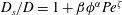
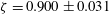
 $\unicode[STIX]{x1D6FD}=2.98\pm 0.39$
,
$\unicode[STIX]{x1D6FD}=2.98\pm 0.39$
,
 $\unicode[STIX]{x1D6FC}=1.61\pm 0.26$
and
$\unicode[STIX]{x1D6FC}=1.61\pm 0.26$
and
 $\unicode[STIX]{x1D701}=0.900\pm 0.031$
.
$\unicode[STIX]{x1D701}=0.900\pm 0.031$
.
The paper is structured as follows. In § 2 we introduce an adaptive unstructured finite element method for modelling two-dimensional suspensions at zero Reynolds number, and we discuss the discretization and system set-up in § 3. We then quantify the structures of mixing in the fluid phase in § 4, before we quantify mixing through concentration distributions in § 5, and through the shear-induced self-diffusion coefficient for both phases and at finite Péclet numbers in § 6. We sum up and conclude in § 7.
2 Model description
Numerous numerical techniques have been used to study particle suspensions. Among them we find dissipative particle dynamics (Hoogerbrugge & Koelman Reference Hoogerbrugge and Koelman1992), the lattice Boltzmann method (Ladd & Verberg Reference Ladd and Verberg2001) as well as the Lagrange multiplier fictitious domain method (Glowinski et al. Reference Glowinski, Pan, Hesla and Joseph1999) and the finite element method (Maury Reference Maury1999). The most widely used technique for suspensions at zero Reynolds number is Stokesian dynamics (Brady & Bossis Reference Brady and Bossis1988; Sierou & Brady Reference Sierou and Brady2001). In this paper, we use a two-dimensional finite element method for rigid non-Brownian fully lubricated particles in Stokes flow (i.e. zero Reynolds number and infinite Péclet number). The implementation is based on MILAMIN (Dabrowski, Krotkiewski & Schmid Reference Dabrowski, Krotkiewski and Schmid2008), which is an efficient open-source implementation of a finite element model Stokes solver in MATLAB; we have used this model previously to investigate the transient nature of suspensions and the statistics of close particle encounters (Thøgersen, Dabrowski & Malthe-Sørenssen Reference Thøgersen, Dabrowski and Malthe-Sørenssen2016).
We solve the incompressible Stokes equations. Conservation of mass yields
 $$\begin{eqnarray}\unicode[STIX]{x1D735}\boldsymbol{\cdot }\boldsymbol{v}=0,\end{eqnarray}$$
where
 $\boldsymbol{v}$
is the velocity field. Conservation of momentum yields
$\boldsymbol{v}$
is the velocity field. Conservation of momentum yields
 $$\begin{eqnarray}\unicode[STIX]{x1D735}\boldsymbol{\cdot }\unicode[STIX]{x1D748}=\mathbf{0},\end{eqnarray}$$
where
 $\mathbf{0}$
ensures a neutrally buoyant suspension. Here
$\mathbf{0}$
ensures a neutrally buoyant suspension. Here
 $\unicode[STIX]{x1D748}$
is the stress tensor,
$\unicode[STIX]{x1D748}$
is the stress tensor,
 $$\begin{eqnarray}\unicode[STIX]{x1D748}=-p\unicode[STIX]{x1D644}+\unicode[STIX]{x1D64F},\end{eqnarray}$$
where
 $p$
is the pressure,
$p$
is the pressure,
 $\unicode[STIX]{x1D644}$
is the identity matrix and
$\unicode[STIX]{x1D644}$
is the identity matrix and
 $$\begin{eqnarray}\unicode[STIX]{x1D64F}=\unicode[STIX]{x1D707}(\unicode[STIX]{x1D735}\boldsymbol{v}+(\unicode[STIX]{x1D735}\boldsymbol{v})^{\text{T}})\end{eqnarray}$$
is the deviatoric stress tensor.
We introduce an approximation space through a set of basis functions for velocity and pressure, which are usually called shape functions. We use a mixed formulation finite element method and the seven-node Crouzeix–Raviart triangular element (Crouzeix & Raviart Reference Crouzeix and Raviart1973). We use
 $N_{i}$
to denote continuous shape functions for velocity, and
$N_{i}$
to denote continuous shape functions for velocity, and
 $\unicode[STIX]{x1D6F1}_{i}$
for linear discontinuous shape functions for pressure. Approximations of velocities and pressure marked with
$\unicode[STIX]{x1D6F1}_{i}$
for linear discontinuous shape functions for pressure. Approximations of velocities and pressure marked with
 $\tilde{~}$
are then
$\tilde{~}$
are then
 $$\begin{eqnarray}\tilde{v}_{x}(x,y)=\mathop{\sum }_{i=1}^{nnod}N_{i}(x,y)v_{x,i},\end{eqnarray}$$
 $$\begin{eqnarray}\tilde{v}_{y}(x,y)=\mathop{\sum }_{i=1}^{nnod}N_{i}(x,y)v_{y,i},\end{eqnarray}$$
and
 $$\begin{eqnarray}\tilde{p}(x,y)=\mathop{\sum }_{i=1}^{np}\unicode[STIX]{x1D6F1}_{i}(x,y)p_{i},\end{eqnarray}$$
where
 $nnod$
and
$nnod$
and
 $np$
are the number of velocity and pressure degrees of freedom, respectively. In Voigt notation, we define the following quantities at the element level:
$np$
are the number of velocity and pressure degrees of freedom, respectively. In Voigt notation, we define the following quantities at the element level:
 $$\begin{eqnarray}\unicode[STIX]{x1D63D}_{el}=\left(\begin{array}{@{}ccc@{}}{\displaystyle \frac{\unicode[STIX]{x2202}N_{1}}{\unicode[STIX]{x2202}x}} & 0 & \cdots \\ 0 & {\displaystyle \frac{\unicode[STIX]{x2202}N_{1}}{\unicode[STIX]{x2202}y}} & \cdots \\ {\displaystyle \frac{\unicode[STIX]{x2202}N_{1}}{\unicode[STIX]{x2202}y}} & {\displaystyle \frac{\unicode[STIX]{x2202}N_{1}}{\unicode[STIX]{x2202}x}} & \cdots \\ \end{array}\right),\end{eqnarray}$$
 $$\begin{eqnarray}\unicode[STIX]{x1D63F}_{el}=\unicode[STIX]{x1D707}\left(\begin{array}{@{}ccc@{}}\frac{4}{3} & -\frac{2}{3} & 0\\ -\frac{2}{3} & \frac{4}{3} & 0\\ 0 & 0 & 1\end{array}\right),\end{eqnarray}$$
 $$\begin{eqnarray}\unicode[STIX]{x1D72B}_{el}=\left(\begin{array}{@{}cccc@{}}\unicode[STIX]{x1D6F1}_{1} & \unicode[STIX]{x1D6F1}_{2} & \unicode[STIX]{x1D6F1}_{3} & \cdots \end{array}\right),\end{eqnarray}$$
 $$\begin{eqnarray}\unicode[STIX]{x1D63E}_{el}=\left(\begin{array}{@{}ccc@{}}{\displaystyle \frac{\unicode[STIX]{x2202}N_{1}}{\unicode[STIX]{x2202}x}} & {\displaystyle \frac{\unicode[STIX]{x2202}N_{1}}{\unicode[STIX]{x2202}y}} & \cdots \\ \end{array}\right).\end{eqnarray}$$
The weak formulation of Stokes equations can then be written through the following matrices:
 $$\begin{eqnarray}\unicode[STIX]{x1D63C}_{el}=\iint _{\unicode[STIX]{x1D6FA}}\unicode[STIX]{x1D63D}_{el}^{\text{T}}\unicode[STIX]{x1D63F}_{el}\unicode[STIX]{x1D63D}_{el}\,\text{dx}\,\text{dy},\end{eqnarray}$$
 $$\begin{eqnarray}\unicode[STIX]{x1D64C}_{el}=\iint _{\unicode[STIX]{x1D6FA}}\unicode[STIX]{x1D72B}_{el}\unicode[STIX]{x1D63E}_{el}^{\text{T}}\,\text{dx}\,\text{dy},\end{eqnarray}$$
and
 $$\begin{eqnarray}\unicode[STIX]{x1D648}_{el}=\iint _{\unicode[STIX]{x1D6FA}}\unicode[STIX]{x1D72B}_{el}\unicode[STIX]{x1D72B}_{el}^{\text{T}}\,\text{dx}\,\text{dy},\end{eqnarray}$$
where the integrals over the domain
 $\unicode[STIX]{x1D6FA}$
are carried out at an element level. Using isoparametric elements, the elements are mapped onto a fixed reference frame in the local coordinates
$\unicode[STIX]{x1D6FA}$
are carried out at an element level. Using isoparametric elements, the elements are mapped onto a fixed reference frame in the local coordinates
 $[\unicode[STIX]{x1D712},\unicode[STIX]{x1D701}]$
. The derivatives of the shape functions of global coordinates
$[\unicode[STIX]{x1D712},\unicode[STIX]{x1D701}]$
. The derivatives of the shape functions of global coordinates
 $x$
and
$x$
and
 $y$
are found from the derivatives of the shape functions with respect to the local coordinates:
$y$
are found from the derivatives of the shape functions with respect to the local coordinates:
 $$\begin{eqnarray}\left\{\frac{\unicode[STIX]{x2202}N_{i}}{\unicode[STIX]{x2202}x},\frac{\unicode[STIX]{x2202}N_{i}}{\unicode[STIX]{x2202}y}\right\}=\left\{\frac{\unicode[STIX]{x2202}N_{i}}{\unicode[STIX]{x2202}\unicode[STIX]{x1D712}},\frac{\unicode[STIX]{x2202}N_{i}}{\unicode[STIX]{x2202}\unicode[STIX]{x1D701}}\right\}\unicode[STIX]{x1D645}^{-1},\end{eqnarray}$$
where
 $\unicode[STIX]{x1D645}$
is the Jacobian,
$\unicode[STIX]{x1D645}$
is the Jacobian,
 $$\begin{eqnarray}\unicode[STIX]{x1D645}=\left(\begin{array}{@{}cc@{}}{\displaystyle \frac{\unicode[STIX]{x2202}x}{\unicode[STIX]{x2202}\unicode[STIX]{x1D712}}} & {\displaystyle \frac{\unicode[STIX]{x2202}x}{\unicode[STIX]{x2202}\unicode[STIX]{x1D701}}}\\ {\displaystyle \frac{\unicode[STIX]{x2202}y}{\unicode[STIX]{x2202}\unicode[STIX]{x1D712}}} & {\displaystyle \frac{\unicode[STIX]{x2202}y}{\unicode[STIX]{x2202}\unicode[STIX]{x1D701}}}\end{array}\right).\end{eqnarray}$$
The volume integrals over
 $\unicode[STIX]{x1D6FA}$
are carried out using elementwise quadrature, which yields sums over
$\unicode[STIX]{x1D6FA}$
are carried out using elementwise quadrature, which yields sums over
 $nip$
integration points located at
$nip$
integration points located at
 $[\unicode[STIX]{x1D712}_{k},\unicode[STIX]{x1D701}_{k}]$
:
$[\unicode[STIX]{x1D712}_{k},\unicode[STIX]{x1D701}_{k}]$
:
 $$\begin{eqnarray}\displaystyle & \displaystyle \unicode[STIX]{x1D63C}_{el}=\mathop{\sum }_{k=1}^{nip}W_{k}\left(\unicode[STIX]{x1D63D}_{el}^{\text{T}}\unicode[STIX]{x1D63F}_{el}\unicode[STIX]{x1D63D}_{el}|\unicode[STIX]{x1D645}|\right)_{[\unicode[STIX]{x1D712}_{k},\unicode[STIX]{x1D701}_{k}]}, & \displaystyle\end{eqnarray}$$
 $$\begin{eqnarray}\displaystyle & \displaystyle \unicode[STIX]{x1D64C}_{el}=\mathop{\sum }_{k=1}^{nip}W_{k}\left(\unicode[STIX]{x1D72B}_{el}^{\text{T}}\unicode[STIX]{x1D63E}_{el}|\unicode[STIX]{x1D645}|\right)_{[\unicode[STIX]{x1D712}_{k},\unicode[STIX]{x1D701}_{k}]}, & \displaystyle\end{eqnarray}$$
 $$\begin{eqnarray}\displaystyle & \displaystyle \unicode[STIX]{x1D648}_{el}=\mathop{\sum }_{k=1}^{nip}W_{k}\left(\unicode[STIX]{x1D72B}_{el}^{\text{T}}\unicode[STIX]{x1D72B}_{el}|\unicode[STIX]{x1D645}|\right)_{[\unicode[STIX]{x1D712}_{k},\unicode[STIX]{x1D701}_{k}]}, & \displaystyle\end{eqnarray}$$
where
 $|\unicode[STIX]{x1D645}|$
is the Jacobian determinant, and
$|\unicode[STIX]{x1D645}|$
is the Jacobian determinant, and
 $W_{k}$
are integration point specific weights. Using a weighted residual Galerkin method yields a symmetric, albeit indefinite, matrix equation. The full matrix assembly yields the global matrix equation, where we use the augmented Lagrangian method and solve
$W_{k}$
are integration point specific weights. Using a weighted residual Galerkin method yields a symmetric, albeit indefinite, matrix equation. The full matrix assembly yields the global matrix equation, where we use the augmented Lagrangian method and solve
 $$\begin{eqnarray}\left(\begin{array}{@{}cc@{}}\unicode[STIX]{x1D63C}+\unicode[STIX]{x1D706}\unicode[STIX]{x1D64C}\unicode[STIX]{x1D648}^{-1}\unicode[STIX]{x1D64C}^{\text{T}} & \unicode[STIX]{x1D64C}\\ \unicode[STIX]{x1D64C}^{\text{T}} & 0\\ \end{array}\right)\left(\begin{array}{@{}c@{}}v\\ p\end{array}\right)=\left(\begin{array}{@{}c@{}}g\\ h\end{array}\right).\end{eqnarray}$$
Here, we have introduced the general term
 $[\boldsymbol{g},\boldsymbol{h}]$
for the right-hand side after boundary conditions have been applied. In practice,
$[\boldsymbol{g},\boldsymbol{h}]$
for the right-hand side after boundary conditions have been applied. In practice,
 $$\begin{eqnarray}\unicode[STIX]{x1D64C}^{\text{T}}(\unicode[STIX]{x1D63C}+\unicode[STIX]{x1D706}\unicode[STIX]{x1D64C}\unicode[STIX]{x1D648}^{-1}\unicode[STIX]{x1D64C}^{\text{T}})^{-1}\unicode[STIX]{x1D64C}p=\unicode[STIX]{x1D64C}^{\text{T}}(\unicode[STIX]{x1D63C}+\unicode[STIX]{x1D706}\unicode[STIX]{x1D64C}\unicode[STIX]{x1D648}^{-1}\unicode[STIX]{x1D64C}^{\text{T}})^{-1}g-h\end{eqnarray}$$
is solved iteratively for
 $p$
using a preconditioned conjugate gradient method, with
$p$
using a preconditioned conjugate gradient method, with
 $\unicode[STIX]{x1D648}$
as the preconditioner. Since the pressures shape functions are discontinuous,
$\unicode[STIX]{x1D648}$
as the preconditioner. Since the pressures shape functions are discontinuous,
 $\unicode[STIX]{x1D648}^{-1}$
can be obtained at the element level, which improves performance significantly. For the augmented matrix
$\unicode[STIX]{x1D648}^{-1}$
can be obtained at the element level, which improves performance significantly. For the augmented matrix
 $\unicode[STIX]{x1D63C}+\unicode[STIX]{x1D706}\unicode[STIX]{x1D64C}\unicode[STIX]{x1D648}^{-1}\unicode[STIX]{x1D64C}^{\text{T}}$
, we use Cholesky decomposition, which only has to be carried out once, so that the incremental steps can be calculated efficiently using the method of backward–forward substitution. The resulting incompressible velocity field can be recovered from
$\unicode[STIX]{x1D63C}+\unicode[STIX]{x1D706}\unicode[STIX]{x1D64C}\unicode[STIX]{x1D648}^{-1}\unicode[STIX]{x1D64C}^{\text{T}}$
, we use Cholesky decomposition, which only has to be carried out once, so that the incremental steps can be calculated efficiently using the method of backward–forward substitution. The resulting incompressible velocity field can be recovered from
 $$\begin{eqnarray}v=(\unicode[STIX]{x1D63C}+\unicode[STIX]{x1D706}\unicode[STIX]{x1D64C}\unicode[STIX]{x1D648}^{-1}\unicode[STIX]{x1D64C}^{\text{T}})^{-1}(g-\unicode[STIX]{x1D64C}p).\end{eqnarray}$$
For a more detailed discussion about implementation and optimization procedures, we refer to Dabrowski et al. (Reference Dabrowski, Krotkiewski and Schmid2008).
The rigidity of particles is enforced directly on the matrix level through a matrix transformation. Using an operator
 $\unicode[STIX]{x1D64B}$
, we replace
$\unicode[STIX]{x1D64B}$
, we replace
 $\unicode[STIX]{x1D63C}$
,
$\unicode[STIX]{x1D63C}$
,
 $\unicode[STIX]{x1D64C}$
and
$\unicode[STIX]{x1D64C}$
and
 $\boldsymbol{g}$
in (2.20) with
$\boldsymbol{g}$
in (2.20) with
 $$\begin{eqnarray}\unicode[STIX]{x1D63C}_{p}=\unicode[STIX]{x1D64B}^{\text{T}}\unicode[STIX]{x1D63C}\unicode[STIX]{x1D64B},\end{eqnarray}$$
 $$\begin{eqnarray}\unicode[STIX]{x1D64C}_{p}=\unicode[STIX]{x1D64C}\unicode[STIX]{x1D64B}\end{eqnarray}$$
and
 $$\begin{eqnarray}\boldsymbol{g}_{p}=\unicode[STIX]{x1D64B}^{\text{T}}\boldsymbol{g},\end{eqnarray}$$
respectively. The resulting matrix equation is still symmetric and positive definite, and ensures that the net forces and torques on the particles vanish. The particle motion is fully coupled to the velocity field of the fluid phase, as we solve for all velocities simultaneously. Note that there are no constraints on the particle shape, as long as the particle centre of mass is given. The operator
 $\unicode[STIX]{x1D64B}$
can be found in appendix A. Validation of the implementation can be found in appendix B.
$\unicode[STIX]{x1D64B}$
can be found in appendix A. Validation of the implementation can be found in appendix B.
3 Discretization and system set-up
Direct modelling of particle suspensions is numerically challenging. In particular, in finite element models with unstructured body-fitting meshes, particle overlaps is a problem if we wish to run systems to very large strains. Increasing the resolution between particles is crucial for accuracy, but, since particles can be arbitrarily close, this may lead to unconstrained computational costs, and ill-conditioned systems of equations due to numerous small elements in between close particle pairs. Still, mesh refinement in particle apertures as well as a small enough time step make it possible to run the system to large enough strains to address shear-induced self-diffusion for particle volume fractions up to
 $\unicode[STIX]{x1D719}=0.4$
, without introducing any artificial repulsive forces between the particles.
$\unicode[STIX]{x1D719}=0.4$
, without introducing any artificial repulsive forces between the particles.
In this paper we study the purely hydrodynamic limit without repulsive forces between the particles. In order to achieve this, special care has to be taken over spatial discretization as well as over time integration. We generate an unstructured triangular mesh at every time step using ‘Triangle’ (Shewchuk Reference Shewchuk1996), and use adaptive mesh refinement to ensure that there are at least two mesh elements between all particle pairs at any time during the simulation. In this way we ensure that the velocity field is accurately computed between close particles (quadratic velocity profiles can be represented within a single triangular element). For time integration we use the second-order Runge–Kutta method with time step
 $\dot{\unicode[STIX]{x1D6FE}}\,\text{d}t=0.02$
. If particle overlap is detected, the simulation is terminated, which for dense suspensions sets limits on the maximum strains that we can reach. For statistical measures, it would be beneficial to have one very long run rather than ensemble averaging over multiple shorter ones, but due to computational challenges the latter is used throughout the paper.
$\dot{\unicode[STIX]{x1D6FE}}\,\text{d}t=0.02$
. If particle overlap is detected, the simulation is terminated, which for dense suspensions sets limits on the maximum strains that we can reach. For statistical measures, it would be beneficial to have one very long run rather than ensemble averaging over multiple shorter ones, but due to computational challenges the latter is used throughout the paper.
A strength of the finite element method is that it allows access to the velocity field in the fluid at all time steps. This means that, in addition to measuring the shear-induced self-diffusion of the solid phase, we can also measure the shear-induced self-diffusivity of the fluid phase using the fluid velocity field. While we acknowledge that particle shape can play a role in migration of particles (Rusconi & Stone Reference Rusconi and Stone2008), we limit this study to monodisperse discs.
The system set-up is demonstrated in figure 1. We use a simulation box with dimensions
 $L\times L$
. The left and right boundaries are periodic (the rows and columns of the corresponding periodic degrees of freedom are replaced by their sums in the system of equations (2.20)), and we set up a shear rate
$L\times L$
. The left and right boundaries are periodic (the rows and columns of the corresponding periodic degrees of freedom are replaced by their sums in the system of equations (2.20)), and we set up a shear rate
 $\dot{\unicode[STIX]{x1D6FE}}$
in the
$\dot{\unicode[STIX]{x1D6FE}}$
in the
 $x$
-direction by applying Dirichlet boundary conditions at the top and bottom boundaries: constant
$x$
-direction by applying Dirichlet boundary conditions at the top and bottom boundaries: constant
 $v_{x}$
and zero
$v_{x}$
and zero
 $v_{y}$
. The strain
$v_{y}$
. The strain
 $\unicode[STIX]{x1D6FE}=\dot{\unicode[STIX]{x1D6FE}}\,\text{d}t$
is then the dimensionless time in the system. We initialize the system of particles using random sequential adsorption (Widom Reference Widom1966), with a small initial particle radius. We then increase the radius of the particles and iterate until no overlaps are present using a steepest descent algorithm.
$\unicode[STIX]{x1D6FE}=\dot{\unicode[STIX]{x1D6FE}}\,\text{d}t$
is then the dimensionless time in the system. We initialize the system of particles using random sequential adsorption (Widom Reference Widom1966), with a small initial particle radius. We then increase the radius of the particles and iterate until no overlaps are present using a steepest descent algorithm.
Figure 2 shows a snapshot of a simulation of
 $N=4096$
particles at volume fraction
$N=4096$
particles at volume fraction
 $\unicode[STIX]{x1D719}=0.3$
in simple shear. The presence of particles perturbs the velocity field and sets up a non-zero velocity field in the
$\unicode[STIX]{x1D719}=0.3$
in simple shear. The presence of particles perturbs the velocity field and sets up a non-zero velocity field in the
 $y$
-direction, both for the particles and for the fluid. In figure 2(c) one can see a low-velocity layer (
$y$
-direction, both for the particles and for the fluid. In figure 2(c) one can see a low-velocity layer (
 $y$
-component) close to the boundary that is approximately two particle diameters thick. In bounded domains, one can also find swapping trajectories (Zurita-Gotor, Bławzdziewicz & Wajnryb Reference Zurita-Gotor, Bławzdziewicz and Wajnryb2007) as well as layered hexagonal structures close to the boundaries (Gallier et al.
Reference Gallier, Lemaire, Lobry and Peters2016). Layers of low velocity close to the boundary introduce boundary effects on measurements of mean square displacement as well as shear-induced self-diffusion that scale with
$y$
-component) close to the boundary that is approximately two particle diameters thick. In bounded domains, one can also find swapping trajectories (Zurita-Gotor, Bławzdziewicz & Wajnryb Reference Zurita-Gotor, Bławzdziewicz and Wajnryb2007) as well as layered hexagonal structures close to the boundaries (Gallier et al.
Reference Gallier, Lemaire, Lobry and Peters2016). Layers of low velocity close to the boundary introduce boundary effects on measurements of mean square displacement as well as shear-induced self-diffusion that scale with
 $1/\sqrt{N}$
. Throughout this paper we will use the scaling with
$1/\sqrt{N}$
. Throughout this paper we will use the scaling with
 $1/\sqrt{N}$
when we look at measurements towards infinite system sizes. An alternative approach that was taken by Gallier et al. (Reference Gallier, Lemaire, Peters and Lobry2014) is to perform measurements in the core region (mid 50 %) in order to remove boundary effects. Figure 3 shows the probability density of the fluid velocity field for systems of
$1/\sqrt{N}$
when we look at measurements towards infinite system sizes. An alternative approach that was taken by Gallier et al. (Reference Gallier, Lemaire, Peters and Lobry2014) is to perform measurements in the core region (mid 50 %) in order to remove boundary effects. Figure 3 shows the probability density of the fluid velocity field for systems of
 $N=1024$
and
$N=1024$
and
 $\unicode[STIX]{x1D719}\in [0.1,0.4]$
equilibrated for
$\unicode[STIX]{x1D719}\in [0.1,0.4]$
equilibrated for
 $\dot{\unicode[STIX]{x1D6FE}}t=20$
from simulations of
$\dot{\unicode[STIX]{x1D6FE}}t=20$
from simulations of
 $4\times 10^{4}$
fluid tracer particles integrated forward in time with a second-order Adams–Bashforth method with time step
$4\times 10^{4}$
fluid tracer particles integrated forward in time with a second-order Adams–Bashforth method with time step
 $\dot{\unicode[STIX]{x1D6FE}}\,\text{d}t=0.02$
. The boundary effects have been removed by removing tracers in a band of width
$\dot{\unicode[STIX]{x1D6FE}}\,\text{d}t=0.02$
. The boundary effects have been removed by removing tracers in a band of width
 $4r$
near the top and bottom boundaries.
$4r$
near the top and bottom boundaries.

Figure 1. Sketch of the system set-up. The left and right boundaries are periodic, while the top and bottom boundaries have velocities in opposite directions to give a background shear rate
 $\dot{\unicode[STIX]{x1D6FE}}$
. The particle configuration is a snapshot from a simulation of
$\dot{\unicode[STIX]{x1D6FE}}$
. The particle configuration is a snapshot from a simulation of
 $N=1024$
particles at volume fraction
$N=1024$
particles at volume fraction
 $\unicode[STIX]{x1D719}=0.4$
at
$\unicode[STIX]{x1D719}=0.4$
at
 $\unicode[STIX]{x1D6FE}=30$
.
$\unicode[STIX]{x1D6FE}=30$
.

Figure 2. Snapshot of simulation at
 $\unicode[STIX]{x1D6FE}=30$
of 4096 particles at volume fraction
$\unicode[STIX]{x1D6FE}=30$
of 4096 particles at volume fraction
 $\unicode[STIX]{x1D719}=0.3$
in simple shear. The top and bottom boundaries have fixed velocities in the
$\unicode[STIX]{x1D719}=0.3$
in simple shear. The top and bottom boundaries have fixed velocities in the
 $x$
-direction, while the left and right boundaries are periodic. (a) The
$x$
-direction, while the left and right boundaries are periodic. (a) The
 $x$
-component of the velocity field. (b) Close-up of the
$x$
-component of the velocity field. (b) Close-up of the
 $x$
-component of the velocity field with subtracted background shear rate. (c) Close-up of the
$x$
-component of the velocity field with subtracted background shear rate. (c) Close-up of the
 $y$
-component of the velocity field. The presence of particles sets up a non-zero
$y$
-component of the velocity field. The presence of particles sets up a non-zero
 $y$
-component of the velocity field, leading to shear-induced self-diffusion of particles as well as of the surrounding fluid. (d) Close-up of the curl field
$y$
-component of the velocity field, leading to shear-induced self-diffusion of particles as well as of the surrounding fluid. (d) Close-up of the curl field
 $\boldsymbol{e}_{z}\boldsymbol{\cdot }\unicode[STIX]{x1D735}\times \boldsymbol{v}$
, where
$\boldsymbol{e}_{z}\boldsymbol{\cdot }\unicode[STIX]{x1D735}\times \boldsymbol{v}$
, where
 $\boldsymbol{e}_{z}$
is the unit vector out of the plane.
$\boldsymbol{e}_{z}$
is the unit vector out of the plane.

Figure 3. Probability density of the fluid velocity field for
 $N=1024$
and
$N=1024$
and
 $\unicode[STIX]{x1D719}\in [0.1,0.4]$
. (a) The
$\unicode[STIX]{x1D719}\in [0.1,0.4]$
. (a) The
 $y$
-component of the velocity field scaled with the shear rate
$y$
-component of the velocity field scaled with the shear rate
 $\dot{\unicode[STIX]{x1D6FE}}$
and the particle radius
$\dot{\unicode[STIX]{x1D6FE}}$
and the particle radius
 $r$
. (b) The
$r$
. (b) The
 $x$
-component of the velocity field scaled with the shear rate
$x$
-component of the velocity field scaled with the shear rate
 $\dot{\unicode[STIX]{x1D6FE}}$
and the system size
$\dot{\unicode[STIX]{x1D6FE}}$
and the system size
 $L$
. (c) The
$L$
. (c) The
 $x$
-component of the velocity, where the background velocity field
$x$
-component of the velocity, where the background velocity field
 $\dot{\unicode[STIX]{x1D6FE}}y$
has been subtracted, scaled with the shear rate
$\dot{\unicode[STIX]{x1D6FE}}y$
has been subtracted, scaled with the shear rate
 $\dot{\unicode[STIX]{x1D6FE}}$
and the particle radius
$\dot{\unicode[STIX]{x1D6FE}}$
and the particle radius
 $r$
. (The breaking of symmetry in panel (c) is a system size effect, which becomes evident when the particle concentration is not perfectly constant in the
$r$
. (The breaking of symmetry in panel (c) is a system size effect, which becomes evident when the particle concentration is not perfectly constant in the
 $y$
-direction. Since shear-induced self-diffusion is slow, the average shear rate is not always identical to
$y$
-direction. Since shear-induced self-diffusion is slow, the average shear rate is not always identical to
 $\dot{\unicode[STIX]{x1D6FE}}y$
for finite strains.)
$\dot{\unicode[STIX]{x1D6FE}}y$
for finite strains.)

Figure 4. Fluid mixing in a system with
 $N=512$
,
$N=512$
,
 $\unicode[STIX]{x1D719}=0.3$
at
$\unicode[STIX]{x1D719}=0.3$
at
 $Pe=10^{4}$
. The concentration profile is estimated using the diffusive strip method. The dimensions of the window are
$Pe=10^{4}$
. The concentration profile is estimated using the diffusive strip method. The dimensions of the window are
 $(0.2\times 0.2)L$
in the central part of the simulation box.
$(0.2\times 0.2)L$
in the central part of the simulation box.

Figure 5. Fluid tracer concentration field calculated using the diffusive strip method. The concentration profiles are snapshots of a simulation at
 $\unicode[STIX]{x1D6FE}=10$
for
$\unicode[STIX]{x1D6FE}=10$
for
 $N=512$
,
$N=512$
,
 $\unicode[STIX]{x1D719}=0.3$
for
$\unicode[STIX]{x1D719}=0.3$
for
 $Pe=10^{3}$
,
$Pe=10^{3}$
,
 $10^{4}$
,
$10^{4}$
,
 $10^{5}$
and
$10^{5}$
and
 $10^{6}$
. The dimensions of the window are
$10^{6}$
. The dimensions of the window are
 $(0.6\times 0.2)L$
in the central part of the simulation box.
$(0.6\times 0.2)L$
in the central part of the simulation box.

Figure 6. Fluid tracer concentration field calculated using the diffusive strip method. The concentration profiles are snapshots of a simulation at
 $\unicode[STIX]{x1D6FE}=10$
for
$\unicode[STIX]{x1D6FE}=10$
for
 $N=512$
,
$N=512$
,
 $Pe=10^{4}$
for
$Pe=10^{4}$
for
 $\unicode[STIX]{x1D719}=0.1$
,
$\unicode[STIX]{x1D719}=0.1$
,
 $0.2$
,
$0.2$
,
 $0.3$
and
$0.3$
and
 $0.4$
. The dimensions of the window are
$0.4$
. The dimensions of the window are
 $(0.6\times 0.2)L$
in the central part of the simulation box.
$(0.6\times 0.2)L$
in the central part of the simulation box.
4 Structure of mixing in the fluid phase
While we assume that the particle Péclet number is infinite, we assume that diffusion of mass is present in the fluid phase. Recent experiments by Souzy et al. (Reference Souzy, Yin, Villermaux, Abid and Metzger2015) have shown complex structures in the fluid phase when a strip of dye is placed near the boundary in a sheared suspension. Here, we introduce finite fluid tracer Péclet numbers
 $Pe=\dot{\unicode[STIX]{x1D6FE}}r^{2}/D$
, where
$Pe=\dot{\unicode[STIX]{x1D6FE}}r^{2}/D$
, where
 $D$
is the fluid tracer diffusivity,
$D$
is the fluid tracer diffusivity,
 $r$
is the particle radius and
$r$
is the particle radius and
 $\dot{\unicode[STIX]{x1D6FE}}$
is the shear rate. We take advantage of the velocity fields that we calculate using finite elements, and use the diffusive strip method developed by Meunier & Villermaux (Reference Meunier and Villermaux2010), which allows us to study filaments of fluid tracer particles at finite Péclet numbers with strain.
$\dot{\unicode[STIX]{x1D6FE}}$
is the shear rate. We take advantage of the velocity fields that we calculate using finite elements, and use the diffusive strip method developed by Meunier & Villermaux (Reference Meunier and Villermaux2010), which allows us to study filaments of fluid tracer particles at finite Péclet numbers with strain.
4.1 Diffusive strip
To capture the structures, we initialize high-resolution lines of markers and advect them passively with the fluid velocity field set up by the particles. As the line of markers is stretched, we use linear interpolation to add points to it, with a resolution of
 $\text{d}x=5\times 10^{-4}\,L$
. As the lengths of the lines grow fairly fast, it sets limits to the strains we can reach with this method. In the following, we present results up to
$\text{d}x=5\times 10^{-4}\,L$
. As the lengths of the lines grow fairly fast, it sets limits to the strains we can reach with this method. In the following, we present results up to
 $\unicode[STIX]{x1D6FE}=15$
. Compared to a more complex refinement procedure, this could cause some errors at points where the curvature is high (Meunier & Villermaux Reference Meunier and Villermaux2010). However, the resolution used here is fairly high, so we expect these errors to be minor for
$\unicode[STIX]{x1D6FE}=15$
. Compared to a more complex refinement procedure, this could cause some errors at points where the curvature is high (Meunier & Villermaux Reference Meunier and Villermaux2010). However, the resolution used here is fairly high, so we expect these errors to be minor for
 $\unicode[STIX]{x1D6FE}\leqslant 15$
.
$\unicode[STIX]{x1D6FE}\leqslant 15$
.
We insert horizontal filaments with initial concentration
 $c_{0}$
and thickness
$c_{0}$
and thickness
 $s_{0}=1\times 10^{-4}\,L$
in the fluid phase, and integrate their position forward in time. The concentration field
$s_{0}=1\times 10^{-4}\,L$
in the fluid phase, and integrate their position forward in time. The concentration field
 $c(\boldsymbol{x})$
can then be reconstructed from
$c(\boldsymbol{x})$
can then be reconstructed from
 $$\begin{eqnarray}c(\boldsymbol{x})=\mathop{\sum }_{i}\frac{c_{0}/1.7726}{\sqrt{1+4\unicode[STIX]{x1D70F}_{i}(t)}}\exp \left[-\frac{\left((\boldsymbol{x}-\boldsymbol{c}_{i})\boldsymbol{\cdot }\unicode[STIX]{x1D748}_{i}\right)^{2}}{\unicode[STIX]{x0394}l^{2}}-\frac{\left((\boldsymbol{x}-\boldsymbol{c}_{i})\boldsymbol{\cdot }\boldsymbol{n}_{i}\right)^{2}}{s_{i}^{2}(1+4\unicode[STIX]{x1D70F}_{i}(t))}\right],\end{eqnarray}$$
where
 $\boldsymbol{n}$
and
$\boldsymbol{n}$
and
 $\unicode[STIX]{x1D748}$
are unit vectors normal and tangential to the strip,
$\unicode[STIX]{x1D748}$
are unit vectors normal and tangential to the strip,
 $$\begin{eqnarray}s_{i}=s_{0}\frac{\unicode[STIX]{x0394}x_{i}^{0}}{\unicode[STIX]{x0394}x_{i}}\end{eqnarray}$$
is the local elongation of the strip, and the dimensionless time
 $\unicode[STIX]{x1D70F}_{i}$
is found through
$\unicode[STIX]{x1D70F}_{i}$
is found through
 $$\begin{eqnarray}\frac{\text{d}\unicode[STIX]{x1D70F}_{i}}{\text{d}t}=\frac{D}{s_{i}(t)^{2}}\end{eqnarray}$$
with the initial condition
 $\unicode[STIX]{x1D70F}_{i}=0$
. In the above,
$\unicode[STIX]{x1D70F}_{i}=0$
. In the above,
 $\unicode[STIX]{x0394}l$
is the distance between the points on the strip, which is reinterpolated to the mean thickness of the strip
$\unicode[STIX]{x0394}l$
is the distance between the points on the strip, which is reinterpolated to the mean thickness of the strip
 $\unicode[STIX]{x0394}l=\left\langle s_{i}\sqrt{1+4\unicode[STIX]{x1D70F}_{i}}\right\rangle$
.
$\unicode[STIX]{x0394}l=\left\langle s_{i}\sqrt{1+4\unicode[STIX]{x1D70F}_{i}}\right\rangle$
.

Figure 7. Sketch of the box counting approach to determine the fractal dimension. The interface structure is covered with boxes of size
 $(l\times l)$
, and the number of boxes
$(l\times l)$
, and the number of boxes
 $N_{b}$
needed to cover the structure is counted. The box size is then reduced and the process repeated. In the end, we end up with the number of boxes as a function of box size,
$N_{b}$
needed to cover the structure is counted. The box size is then reduced and the process repeated. In the end, we end up with the number of boxes as a function of box size,
 $N_{b}(l)$
. The box counting dimension is then determined through (4.4).
$N_{b}(l)$
. The box counting dimension is then determined through (4.4).
The diffusive strip method requires an approximation at the particle rims. Here, we let the line of markers pass through the particles, and then set
 $c_{0}=0$
inside the particles. This allows us to keep the one-dimensional approximation to diffusion at the particle rim. Particle overlaps pose a challenge when modelling the purely hydrodynamic limit. However, for
$c_{0}=0$
inside the particles. This allows us to keep the one-dimensional approximation to diffusion at the particle rim. Particle overlaps pose a challenge when modelling the purely hydrodynamic limit. However, for
 $\unicode[STIX]{x1D6FE}<15$
, we did not encounter problems with lines overlapping, which could be attributed to the high accuracy of the velocity field from the finite element model. For larger strains, we would expect this to become increasingly problematic.
$\unicode[STIX]{x1D6FE}<15$
, we did not encounter problems with lines overlapping, which could be attributed to the high accuracy of the velocity field from the finite element model. For larger strains, we would expect this to become increasingly problematic.
Figure 4 shows the evolution of the fluid mixing as a function of strain for
 $N=512$
and
$N=512$
and
 $\unicode[STIX]{x1D719}=0.3$
at
$\unicode[STIX]{x1D719}=0.3$
at
 $Pe=10^{4}$
(note that the colour bar for
$Pe=10^{4}$
(note that the colour bar for
 $c/c_{0}$
ranges from 0 to 0.1, which is chosen to better visualize the structures). Starting from straight lines in the velocity gradient direction, the lines develop complex structures quite quickly through a series of stretching–folding events, as well as developing filaments that become thinner and increase in length as
$c/c_{0}$
ranges from 0 to 0.1, which is chosen to better visualize the structures). Starting from straight lines in the velocity gradient direction, the lines develop complex structures quite quickly through a series of stretching–folding events, as well as developing filaments that become thinner and increase in length as
 $\unicode[STIX]{x1D6FE}$
increases. Interestingly, the patterns we observe show very close resemblance to the patterns observed in a recent study by Souzy et al. (Reference Souzy, Yin, Villermaux, Abid and Metzger2015) at
$\unicode[STIX]{x1D6FE}$
increases. Interestingly, the patterns we observe show very close resemblance to the patterns observed in a recent study by Souzy et al. (Reference Souzy, Yin, Villermaux, Abid and Metzger2015) at
 $Re=5\times 10^{-3}$
, where they placed a thin layer of dye at one of the walls in a Couette device.
$Re=5\times 10^{-3}$
, where they placed a thin layer of dye at one of the walls in a Couette device.
The effect of the Péclet number is demonstrated in figure 5, which shows snapshots at
 $\unicode[STIX]{x1D6FE}=10$
for a simulation of
$\unicode[STIX]{x1D6FE}=10$
for a simulation of
 $N=512$
particles at
$N=512$
particles at
 $\unicode[STIX]{x1D719}=0.3$
for
$\unicode[STIX]{x1D719}=0.3$
for
 $Pe=10^{3}$
,
$Pe=10^{3}$
,
 $10^{4}$
,
$10^{4}$
,
 $10^{5}$
and
$10^{5}$
and
 $10^{6}$
. Figure 5 demonstrates that the thickness of the filaments is governed by the Péclet number, but that the structure that is forming is in this case well captured also for
$10^{6}$
. Figure 5 demonstrates that the thickness of the filaments is governed by the Péclet number, but that the structure that is forming is in this case well captured also for
 $Pe=10^{3}$
. We will come back to the effects of the Péclet number on enhanced transport properties in § 6.2
$Pe=10^{3}$
. We will come back to the effects of the Péclet number on enhanced transport properties in § 6.2
To investigate the effect of particle volume fraction on the structures that form, we perform diffusive strip simulations for
 $\unicode[STIX]{x1D719}=0.1$
,
$\unicode[STIX]{x1D719}=0.1$
,
 $0.2$
,
$0.2$
,
 $0.3$
and
$0.3$
and
 $0.4$
. Figure 6 shows snapshots at
$0.4$
. Figure 6 shows snapshots at
 $\unicode[STIX]{x1D6FE}=10$
for these different particle volume fractions for a system of
$\unicode[STIX]{x1D6FE}=10$
for these different particle volume fractions for a system of
 $N=512$
particles. From figure 6 it is clear that mixing is more efficient at higher particle volume fractions, which we will also quantify through the shear-induced self-diffusion coefficient in § 6. From figures 4 and 6, it is clear that the structures increase in complexity, not only with increasing strain, but also with increasing particle volume fraction. Using these observations, we will now measure the evolution of the fractal dimension of these structures, and introduce a scaling relation that relates the fractal dimension to the mean square displacement of passive tracers in the fluid phase.
$N=512$
particles. From figure 6 it is clear that mixing is more efficient at higher particle volume fractions, which we will also quantify through the shear-induced self-diffusion coefficient in § 6. From figures 4 and 6, it is clear that the structures increase in complexity, not only with increasing strain, but also with increasing particle volume fraction. Using these observations, we will now measure the evolution of the fractal dimension of these structures, and introduce a scaling relation that relates the fractal dimension to the mean square displacement of passive tracers in the fluid phase.
4.2 Structure characterization
To quantify these patterns we perform systematic simulations consisting of lines of markers for simulations with
 $N\in [256,1024]$
and
$N\in [256,1024]$
and
 $\unicode[STIX]{x1D719}\in [0.1,0.4]$
up to strains of
$\unicode[STIX]{x1D719}\in [0.1,0.4]$
up to strains of
 $\unicode[STIX]{x1D6FE}=15$
, and measure the fractal dimension using box counting (Meakin Reference Meakin1998). For these measurements, we use the line of passive tracers at infinite Péclet number with infinitesimal thickness. The strategy of box counting to measure the fractal dimension is outlined in figure 7; we cover the domain by boxes of size
$\unicode[STIX]{x1D6FE}=15$
, and measure the fractal dimension using box counting (Meakin Reference Meakin1998). For these measurements, we use the line of passive tracers at infinite Péclet number with infinitesimal thickness. The strategy of box counting to measure the fractal dimension is outlined in figure 7; we cover the domain by boxes of size
 $(l\times l)$
, and then count the number of boxes
$(l\times l)$
, and then count the number of boxes
 $N_{b}$
that are needed to cover the structure. This step is performed for
$N_{b}$
that are needed to cover the structure. This step is performed for
 $l\in [L/10^{3},~L/10]$
, and the fractal dimension
$l\in [L/10^{3},~L/10]$
, and the fractal dimension
 $F$
is measured as the power-law exponent of
$F$
is measured as the power-law exponent of
 $N_{b}$
as a function of
$N_{b}$
as a function of
 $l$
:
$l$
:
 $$\begin{eqnarray}F=-\!\left\langle \frac{\text{d}\log N_{b}(l)}{\text{d}\log l}\right\rangle _{l\in [L/10^{3},\,L/10]}.\end{eqnarray}$$
To avoid system size effects in our measurements of
 $F$
, we use five strips of passive tracers in the central part of the domain and average over these. The strips are separated by a distance
$F$
, we use five strips of passive tracers in the central part of the domain and average over these. The strips are separated by a distance
 $\unicode[STIX]{x0394}y/L=1/32$
. Then
$\unicode[STIX]{x0394}y/L=1/32$
. Then
 $F$
is measured as a function of time for a number of
$F$
is measured as a function of time for a number of
 $N$
and
$N$
and
 $\unicode[STIX]{x1D719}$
, and is plotted in figure 8. In line with the observed increase in complexity of the mixing pattern as a function of
$\unicode[STIX]{x1D719}$
, and is plotted in figure 8. In line with the observed increase in complexity of the mixing pattern as a function of
 $\unicode[STIX]{x1D6FE}$
(figure 4), the fractal dimension increases with
$\unicode[STIX]{x1D6FE}$
(figure 4), the fractal dimension increases with
 $\unicode[STIX]{x1D6FE}$
. In addition, we observe that the fractal dimension grows faster for larger values of
$\unicode[STIX]{x1D6FE}$
. In addition, we observe that the fractal dimension grows faster for larger values of
 $\unicode[STIX]{x1D719}$
, consistent with the increasing complexity we observed in figure 6. The fractal dimension of a line is
$\unicode[STIX]{x1D719}$
, consistent with the increasing complexity we observed in figure 6. The fractal dimension of a line is
 $1$
, and for a space-filling structure in two dimensions it is
$1$
, and for a space-filling structure in two dimensions it is
 $2$
, i.e. the fractal dimension is a measure of how well a structure fills space. From this picture, we can derive a simple scaling relation to collapse the data in figure 8.
$2$
, i.e. the fractal dimension is a measure of how well a structure fills space. From this picture, we can derive a simple scaling relation to collapse the data in figure 8.

Figure 8. Fractal dimension
 $F$
measured using the box counting approach in (4.4) as a function of strain for a number of particle numbers
$F$
measured using the box counting approach in (4.4) as a function of strain for a number of particle numbers
 $N$
and particle volume fractions
$N$
and particle volume fractions
 $\unicode[STIX]{x1D719}$
. We obtain a good data collapse by scaling the
$\unicode[STIX]{x1D719}$
. We obtain a good data collapse by scaling the
 $x$
-axis with the mean square displacement of the fluid phase (inset).
$x$
-axis with the mean square displacement of the fluid phase (inset).
Consider two fluid markers with infinitesimal spacing initially. As a strain rate is applied, this introduces an average relative displacement of the two according to the mean square displacement of the fluid. Now consider the rectangle that has the two fluid markers as two of its corners. Its area
 $A$
is proportional to the square root of mean square displacement in the
$A$
is proportional to the square root of mean square displacement in the
 $x$
and
$x$
and
 $y$
directions:
$y$
directions:
 $$\begin{eqnarray}A\sim \sqrt{\langle \unicode[STIX]{x0394}x(t)^{2}\rangle \langle \unicode[STIX]{x0394}y(t)^{2}\rangle }.\end{eqnarray}$$
Since
 $\langle \unicode[STIX]{x0394}x^{2}\rangle$
is largely dominated by the background shear rate, we can simplify this to
$\langle \unicode[STIX]{x0394}x^{2}\rangle$
is largely dominated by the background shear rate, we can simplify this to
 $$\begin{eqnarray}\langle \unicode[STIX]{x0394}x(t)^{2}\rangle \simeq (\dot{\unicode[STIX]{x1D6FE}}t)^{2}\langle \unicode[STIX]{x0394}y(t)^{2}\rangle ,\end{eqnarray}$$
so that
 $$\begin{eqnarray}A\sim \dot{\unicode[STIX]{x1D6FE}}t\langle \unicode[STIX]{x0394}y(t)^{2}\rangle .\end{eqnarray}$$
The scaling of the
 $y$
-axis is found by scaling
$y$
-axis is found by scaling
 $\unicode[STIX]{x0394}y(t)$
with
$\unicode[STIX]{x0394}y(t)$
with
 $r$
. The
$r$
. The
 $\langle \unicode[STIX]{x0394}y(t)^{2}\rangle$
value is measured from simulations of
$\langle \unicode[STIX]{x0394}y(t)^{2}\rangle$
value is measured from simulations of
 $4\times 10^{4}$
passive tracers uniformly distributed in the domain, integrated forward in time with a second-order Adams–Bashforth scheme with
$4\times 10^{4}$
passive tracers uniformly distributed in the domain, integrated forward in time with a second-order Adams–Bashforth scheme with
 $\dot{\unicode[STIX]{x1D6FE}}\,\text{d}t=0.02$
. Comparison of different system sizes introduces the additional scaling with
$\dot{\unicode[STIX]{x1D6FE}}\,\text{d}t=0.02$
. Comparison of different system sizes introduces the additional scaling with
 $\sqrt{N}$
. Note that this is due not to boundary effects in
$\sqrt{N}$
. Note that this is due not to boundary effects in
 $F$
, but to boundary effects in the measurement of the mean square displacement. The strips where we measure the fractal dimension are far from the boundary where boundary effects are negligible. An alternative approach to the introduction of
$F$
, but to boundary effects in the measurement of the mean square displacement. The strips where we measure the fractal dimension are far from the boundary where boundary effects are negligible. An alternative approach to the introduction of
 $\sqrt{N}$
would be to measure the mean square displacement only in the central part of the domain. The final scaling for the evolution of the fractal dimension is then
$\sqrt{N}$
would be to measure the mean square displacement only in the central part of the domain. The final scaling for the evolution of the fractal dimension is then
 $$\begin{eqnarray}F\sim \frac{\dot{\unicode[STIX]{x1D6FE}}t\langle \unicode[STIX]{x0394}y(t)^{2}\rangle }{r^{2}\sqrt{N}}.\end{eqnarray}$$
The fractal dimension of the mixing structure lies between 1 and 2. In our measurements we approximate the interface that passes through particles as lines. Since the interface cannot fill the solid phase, this means that in our case
 $F\in [1,~2-\unicode[STIX]{x1D719}]$
by definition. This is due to the straight segments of the interface drawn through the particles, which have fractal dimension
$F\in [1,~2-\unicode[STIX]{x1D719}]$
by definition. This is due to the straight segments of the interface drawn through the particles, which have fractal dimension
 $F=1$
. Note that this scaling originates from our definition, and that the scaling will be different with a different definition of how we represent the interface in the particles. Combining these simple scaling arguments, we scale the
$F=1$
. Note that this scaling originates from our definition, and that the scaling will be different with a different definition of how we represent the interface in the particles. Combining these simple scaling arguments, we scale the
 $x$
-axis as (4.8) and the
$x$
-axis as (4.8) and the
 $y$
-axis as
$y$
-axis as
 $(F-1)/(1-\unicode[STIX]{x1D719})$
in order to rescale the fractal dimension to
$(F-1)/(1-\unicode[STIX]{x1D719})$
in order to rescale the fractal dimension to
 $[0,1]$
. The data collapse is shown in the inset of figure 8. Given the simplicity of the scaling argument, the collapse is very good, and provides a simple relation between the fractal dimension of the interface and the shear-induced self-diffusivity of the fluid phase.
$[0,1]$
. The data collapse is shown in the inset of figure 8. Given the simplicity of the scaling argument, the collapse is very good, and provides a simple relation between the fractal dimension of the interface and the shear-induced self-diffusivity of the fluid phase.

Figure 9. Probability density of concentration in the fluid phase in the central region
 $(1\times 0.2)L$
from diffusive strip simulations of systems of
$(1\times 0.2)L$
from diffusive strip simulations of systems of
 $N=512$
for various
$N=512$
for various
 $\dot{\unicode[STIX]{x1D6FE}}t$
,
$\dot{\unicode[STIX]{x1D6FE}}t$
,
 $\unicode[STIX]{x1D719}$
and
$\unicode[STIX]{x1D719}$
and
 $Pe$
. (a) Probability density as a function of
$Pe$
. (a) Probability density as a function of
 $c/c_{0}$
for
$c/c_{0}$
for
 $\unicode[STIX]{x1D719}=0.3$
,
$\unicode[STIX]{x1D719}=0.3$
,
 $Pe=10^{4}$
and
$Pe=10^{4}$
and
 $\dot{\unicode[STIX]{x1D6FE}}t$
corresponding to figure 4. (b) Probability density as a function of the inverse concentration
$\dot{\unicode[STIX]{x1D6FE}}t$
corresponding to figure 4. (b) Probability density as a function of the inverse concentration
 $c_{0}/c-1$
for
$c_{0}/c-1$
for
 $\unicode[STIX]{x1D719}=0.3$
,
$\unicode[STIX]{x1D719}=0.3$
,
 $Pe=10^{4}$
and
$Pe=10^{4}$
and
 $\dot{\unicode[STIX]{x1D6FE}}t$
corresponding to figure 4. (c) Probability density as a function of the inverse concentration
$\dot{\unicode[STIX]{x1D6FE}}t$
corresponding to figure 4. (c) Probability density as a function of the inverse concentration
 $c_{0}/c-1$
for
$c_{0}/c-1$
for
 $\unicode[STIX]{x1D719}\in [0.1,0.4]$
at
$\unicode[STIX]{x1D719}\in [0.1,0.4]$
at
 $\dot{\unicode[STIX]{x1D6FE}}t=10$
at
$\dot{\unicode[STIX]{x1D6FE}}t=10$
at
 $Pe=10^{4}$
. (d) Probability density as a function of the inverse concentration
$Pe=10^{4}$
. (d) Probability density as a function of the inverse concentration
 $c_{0}/c-1$
for
$c_{0}/c-1$
for
 $\unicode[STIX]{x1D719}=0.3$
at
$\unicode[STIX]{x1D719}=0.3$
at
 $\dot{\unicode[STIX]{x1D6FE}}t=10$
for
$\dot{\unicode[STIX]{x1D6FE}}t=10$
for
 $Pe\in [10^{3},10^{4}]$
.
$Pe\in [10^{3},10^{4}]$
.
5 Mixing at small strains – concentration distributions from the diffusive strip method
For the strains reached using the diffusive strip method, the shear-induced self-diffusive regime has not been established (see e.g. the velocity autocorrelation function in figure 11). In order to quantify mixing at these strains, we measure the distribution of tracer concentration fields from the previous section as a function of
 $\dot{\unicode[STIX]{x1D6FE}}t$
for various
$\dot{\unicode[STIX]{x1D6FE}}t$
for various
 $\unicode[STIX]{x1D719}$
and
$\unicode[STIX]{x1D719}$
and
 $Pe$
.
$Pe$
.
Figure 9 shows the concentration distribution
 $c_{0}/c$
in the fluid phase for
$c_{0}/c$
in the fluid phase for
 $\dot{\unicode[STIX]{x1D6FE}}t\in [0.02,5]$
,
$\dot{\unicode[STIX]{x1D6FE}}t\in [0.02,5]$
,
 $\unicode[STIX]{x1D719}\in [0.1,0.4]$
and
$\unicode[STIX]{x1D719}\in [0.1,0.4]$
and
 $Pe\in [10^{3},10^{6}]$
. Figure 9(a) shows the concentration distribution for
$Pe\in [10^{3},10^{6}]$
. Figure 9(a) shows the concentration distribution for
 $\unicode[STIX]{x1D719}=0.3$
at
$\unicode[STIX]{x1D719}=0.3$
at
 $Pe=10^{4}$
as
$Pe=10^{4}$
as
 $\dot{\unicode[STIX]{x1D6FE}}t$
increases. The initial distribution is U-shaped, with a peak at
$\dot{\unicode[STIX]{x1D6FE}}t$
increases. The initial distribution is U-shaped, with a peak at
 $c/c_{0}=1$
(as was also described by Meunier & Villermaux (Reference Meunier and Villermaux2010)), which quickly shifts to lower concentrations, and the distribution becomes dominated by the low concentrations between the strips. To highlight instead the changes close to the strip, we also give the probability density of the inverse of the concentration
$c/c_{0}=1$
(as was also described by Meunier & Villermaux (Reference Meunier and Villermaux2010)), which quickly shifts to lower concentrations, and the distribution becomes dominated by the low concentrations between the strips. To highlight instead the changes close to the strip, we also give the probability density of the inverse of the concentration
 $c_{0}/c-1$
(figure 9
b). Then one can clearly see the decay and shift of the peak concentration as a function of
$c_{0}/c-1$
(figure 9
b). Then one can clearly see the decay and shift of the peak concentration as a function of
 $\dot{\unicode[STIX]{x1D6FE}}t$
. Figure 9(c,d) shows the dependence on the concentration probability density at
$\dot{\unicode[STIX]{x1D6FE}}t$
. Figure 9(c,d) shows the dependence on the concentration probability density at
 $\dot{\unicode[STIX]{x1D6FE}}t$
on
$\dot{\unicode[STIX]{x1D6FE}}t$
on
 $\unicode[STIX]{x1D719}$
and
$\unicode[STIX]{x1D719}$
and
 $Pe$
, respectively. Increasing the particle volume fraction shifts the peak concentration and widens the inverse concentration distribution. The same applies on decreasing the Péclet number, which demonstrates a strong dependence on the concentration distribution of fluid tracers even at large
$Pe$
, respectively. Increasing the particle volume fraction shifts the peak concentration and widens the inverse concentration distribution. The same applies on decreasing the Péclet number, which demonstrates a strong dependence on the concentration distribution of fluid tracers even at large
 $Pe$
. This is also clearly visible in figure 5. Interestingly, increasing strain, increasing particle volume fraction and decreasing Péclet number all result in very similar changes to the inverse fluid tracer concentration distribution.
$Pe$
. This is also clearly visible in figure 5. Interestingly, increasing strain, increasing particle volume fraction and decreasing Péclet number all result in very similar changes to the inverse fluid tracer concentration distribution.
We also measure the average concentration averaged over the
 $x$
-direction
$x$
-direction
 $\langle c/c_{0}\rangle _{x}$
as a function of
$\langle c/c_{0}\rangle _{x}$
as a function of
 $\dot{\unicode[STIX]{x1D6FE}}t$
. The shape of the distribution for
$\dot{\unicode[STIX]{x1D6FE}}t$
. The shape of the distribution for
 $Pe=10^{4}$
,
$Pe=10^{4}$
,
 $\unicode[STIX]{x1D719}=0.3$
and
$\unicode[STIX]{x1D719}=0.3$
and
 $N=512$
is shown in figure 10(a). This distribution widens as the strain increases. In order to investigate the effect of
$N=512$
is shown in figure 10(a). This distribution widens as the strain increases. In order to investigate the effect of
 $\unicode[STIX]{x1D719}$
and
$\unicode[STIX]{x1D719}$
and
 $Pe$
, we measure the width of the average concentration as a function of
$Pe$
, we measure the width of the average concentration as a function of
 $\dot{\unicode[STIX]{x1D6FE}}t$
, which we define as the standard deviation of the normalized concentration distribution,
$\dot{\unicode[STIX]{x1D6FE}}t$
, which we define as the standard deviation of the normalized concentration distribution,
 $$\begin{eqnarray}\unicode[STIX]{x1D6E5}_{y}\equiv \text{std}\left(\frac{\langle c/c_{0}\rangle _{x}}{\displaystyle \int _{-L/2}^{L/2}\langle c/c_{0}\rangle _{x}}\right),\end{eqnarray}$$
where
 $\unicode[STIX]{x1D6E5}_{y}$
increases with
$\unicode[STIX]{x1D6E5}_{y}$
increases with
 $\dot{\unicode[STIX]{x1D6FE}}t$
and with increasing
$\dot{\unicode[STIX]{x1D6FE}}t$
and with increasing
 $\unicode[STIX]{x1D719}$
. However, it is more or less independent of
$\unicode[STIX]{x1D719}$
. However, it is more or less independent of
 $Pe$
for
$Pe$
for
 $Pe>10^{3}$
. This demonstrates that, although the probability density of concentration has a clear dependence on
$Pe>10^{3}$
. This demonstrates that, although the probability density of concentration has a clear dependence on
 $Pe$
for
$Pe$
for
 $Pe\in [10^{3},10^{6}]$
, the spatial distribution of concentration measured through
$Pe\in [10^{3},10^{6}]$
, the spatial distribution of concentration measured through
 $\unicode[STIX]{x0394}_{y}$
is largely dominated by advection for
$\unicode[STIX]{x0394}_{y}$
is largely dominated by advection for
 $Pe\geqslant 10^{3}$
.
$Pe\geqslant 10^{3}$
.

Figure 10. (a) Concentration averaged over
 $x$
as a function of
$x$
as a function of
 $y/r$
averaged over nine diffusive strips shifted to
$y/r$
averaged over nine diffusive strips shifted to
 $y/r=0$
at
$y/r=0$
at
 $\dot{\unicode[STIX]{x1D6FE}}t=0$
, for
$\dot{\unicode[STIX]{x1D6FE}}t=0$
, for
 $Pe=10^{4}$
,
$Pe=10^{4}$
,
 $\unicode[STIX]{x1D719}=0.3$
and
$\unicode[STIX]{x1D719}=0.3$
and
 $N=512$
. (b) Width of the average concentration
$N=512$
. (b) Width of the average concentration
 $\unicode[STIX]{x1D6E5}_{y}$
as a function of
$\unicode[STIX]{x1D6E5}_{y}$
as a function of
 $\dot{\unicode[STIX]{x1D6FE}}t$
. The width is taken to be the standard deviation of the normalized average concentration distribution.
$\dot{\unicode[STIX]{x1D6FE}}t$
. The width is taken to be the standard deviation of the normalized average concentration distribution.
6 Mixing at large strains – shear-induced self-diffusion
At large strains, the mixing of particles in a suspension close to equilibrium is described by the self-diffusion coefficient. In this section, we measure the self-diffusion coefficient for both the fluid and the solid phase. Before we measure the diffusion coefficient, we equilibrate the system for
 $\dot{\unicode[STIX]{x1D6FE}}t=20$
, which is chosen because of the decay of the velocity autocorrelation function in the
$\dot{\unicode[STIX]{x1D6FE}}t=20$
, which is chosen because of the decay of the velocity autocorrelation function in the
 $y$
-direction (figure 11
b). This resulting mixing of the particles can be described using the self-diffusion coefficient
$y$
-direction (figure 11
b). This resulting mixing of the particles can be described using the self-diffusion coefficient
 $D_{s}$
. Note that the self-diffusion coefficient is actually a tensor of rank 2 in two-dimensional systems that are not isotropic (see e.g. Breedveld et al.
Reference Breedveld, Van Den Ende, Bosscher, Jongschaap and Mellema2002). In this work we focus on the translation of particles normal to the direction of shear, and in the following,
$D_{s}$
. Note that the self-diffusion coefficient is actually a tensor of rank 2 in two-dimensional systems that are not isotropic (see e.g. Breedveld et al.
Reference Breedveld, Van Den Ende, Bosscher, Jongschaap and Mellema2002). In this work we focus on the translation of particles normal to the direction of shear, and in the following,
 $D_{s}$
will denote this component of the self-diffusion tensor (often denoted
$D_{s}$
will denote this component of the self-diffusion tensor (often denoted
 $D_{s,\langle yy\rangle }$
in the literature). Also note that self-diffusion and collective diffusion are in general two separate quantities. In this paper we discuss self-diffusion normal to the direction of shear only. The interested reader is referred to Leighton & Acrivos (Reference Leighton and Acrivos1987b
), Phillips et al. (Reference Phillips, Armstrong, Brown, Graham and Abbott1992), Marchioro & Acrivos (Reference Marchioro and Acrivos2001), Mauri (Reference Mauri2003), Leshansky & Brady (Reference Leshansky and Brady2005) and Leshansky, Morris & Brady (Reference Leshansky, Morris and Brady2008), for example, for discussions on the collective shear-induced diffusivity.
$D_{s,\langle yy\rangle }$
in the literature). Also note that self-diffusion and collective diffusion are in general two separate quantities. In this paper we discuss self-diffusion normal to the direction of shear only. The interested reader is referred to Leighton & Acrivos (Reference Leighton and Acrivos1987b
), Phillips et al. (Reference Phillips, Armstrong, Brown, Graham and Abbott1992), Marchioro & Acrivos (Reference Marchioro and Acrivos2001), Mauri (Reference Mauri2003), Leshansky & Brady (Reference Leshansky and Brady2005) and Leshansky, Morris & Brady (Reference Leshansky, Morris and Brady2008), for example, for discussions on the collective shear-induced diffusivity.
Three different ways of measuring self-diffusivity are reported in the literature. The simplest one is to determine self-diffusion from the mean square displacement using the Einstein–Smoluchowski relation in one dimension,
 $$\begin{eqnarray}D_{s}=\frac{1}{2}\lim _{t\rightarrow \infty }\frac{\text{d}}{\text{d}t}\langle \unicode[STIX]{x0394}y(t)^{2}\rangle ,\end{eqnarray}$$
where the brackets
 $\langle ~\rangle$
denote an ensemble average over available time intervals of length
$\langle ~\rangle$
denote an ensemble average over available time intervals of length
 $t$
. Equivalently, self-diffusivity can be probed through the integral over the velocity autocorrelation function
$t$
. Equivalently, self-diffusivity can be probed through the integral over the velocity autocorrelation function
 $\text{VACF}=(1/N)\sum _{i=1}^{N}\langle v_{i}^{y}(t^{\prime }),v_{i}^{y}(0)\rangle$
:
$\text{VACF}=(1/N)\sum _{i=1}^{N}\langle v_{i}^{y}(t^{\prime }),v_{i}^{y}(0)\rangle$
:
 $$\begin{eqnarray}D_{s}=\frac{1}{N}\int _{0}^{\infty }\mathop{\sum }_{i=1}^{N}\langle v_{i}^{y}(t^{\prime }),v_{i}^{y}(0)\rangle \,\text{d}t^{\prime }.\end{eqnarray}$$
A third approach that has been used for measuring shear-induced diffusion in suspensions involves the self-dynamic structure factor (Leshansky & Brady Reference Leshansky and Brady2005; Leshansky et al. Reference Leshansky, Morris and Brady2008).
Figure 11 demonstrates the various ways of measuring the self-diffusivity for a system consisting of 512 particles at volume fraction
 $\unicode[STIX]{x1D719}=0.1$
. In order to remove system size effects, we measure the self-diffusivity using the integral over the velocity autocorrelation function for particle numbers
$\unicode[STIX]{x1D719}=0.1$
. In order to remove system size effects, we measure the self-diffusivity using the integral over the velocity autocorrelation function for particle numbers
 $N$
from
$N$
from
 $64$
to
$64$
to
 $1024$
for fractions from
$1024$
for fractions from
 $\unicode[STIX]{x1D719}=0.1$
,
$\unicode[STIX]{x1D719}=0.1$
,
 $0.2$
and
$0.2$
and
 $0.4$
, and up to
$0.4$
, and up to
 $4096$
for
$4096$
for
 $\unicode[STIX]{x1D719}=0.3$
. Assuming that there is a thin layer at the boundary that has a thickness proportional to the particle radius, and that does not contribute to the self-diffusion coefficient because the
$\unicode[STIX]{x1D719}=0.3$
. Assuming that there is a thin layer at the boundary that has a thickness proportional to the particle radius, and that does not contribute to the self-diffusion coefficient because the
 $y$
-component of velocity is small, we expect that the system size effect in the diffusion coefficient will scale as
$y$
-component of velocity is small, we expect that the system size effect in the diffusion coefficient will scale as
 $N^{-1/2}$
. This allows us to extrapolate towards a large particle number as shown in figure 11(d). Figure 12 shows
$N^{-1/2}$
. This allows us to extrapolate towards a large particle number as shown in figure 11(d). Figure 12 shows
 $D_{s}(\unicode[STIX]{x1D719})$
extrapolated towards infinite resolution for volume fractions up to
$D_{s}(\unicode[STIX]{x1D719})$
extrapolated towards infinite resolution for volume fractions up to
 $\unicode[STIX]{x1D719}=0.4$
. The best fit for a power law yields
$\unicode[STIX]{x1D719}=0.4$
. The best fit for a power law yields
 $D_{s}(\unicode[STIX]{x1D719})\sim \unicode[STIX]{x1D719}^{1.38\pm 0.50}$
. We do not expect this relation to hold for volume fractions that approach the jamming threshold where previous studies suggested that
$D_{s}(\unicode[STIX]{x1D719})\sim \unicode[STIX]{x1D719}^{1.38\pm 0.50}$
. We do not expect this relation to hold for volume fractions that approach the jamming threshold where previous studies suggested that
 $D_{s}$
will flatten out at high volume fractions (Breedveld et al.
Reference Breedveld, Van Den Ende, Bosscher, Jongschaap and Mellema2002; Metzger et al.
Reference Metzger, Rahli and Yin2013b
), and, as the system jams, vertical motion is inhibited. However, simulating large volume fractions using finite elements for strains large enough to assess self-diffusion remains a very challenging task numerically. In addition we expect that particle interactions such as friction become increasingly important as the volume fraction increases (Boyer, Guazzelli & Pouliquen Reference Boyer, Guazzelli and Pouliquen2011; Seto et al.
Reference Seto, Mari, Morris and Denn2013).
$D_{s}$
will flatten out at high volume fractions (Breedveld et al.
Reference Breedveld, Van Den Ende, Bosscher, Jongschaap and Mellema2002; Metzger et al.
Reference Metzger, Rahli and Yin2013b
), and, as the system jams, vertical motion is inhibited. However, simulating large volume fractions using finite elements for strains large enough to assess self-diffusion remains a very challenging task numerically. In addition we expect that particle interactions such as friction become increasingly important as the volume fraction increases (Boyer, Guazzelli & Pouliquen Reference Boyer, Guazzelli and Pouliquen2011; Seto et al.
Reference Seto, Mari, Morris and Denn2013).
Table 1. Shear-induced self-diffusivity compared to three-dimensional simulations from Sierou & Brady (Reference Sierou and Brady2004) where they used accelerated Stokesian dynamics (ASD). The results from Sierou & Brady match experimental measurements fairly well, although there are large variations of self-diffusivities measured from experiments. Our measured finite element method (FEM) results are systematically higher, which is expected for a two-dimensional system.

In table 1,
 $D_{s}$
obtained from our simulations are shown along with one example from Sierou & Brady (Reference Sierou and Brady2004) in three dimensions using accelerated Stokesian dynamics simulations. Qualitatively, our results show similar
$D_{s}$
obtained from our simulations are shown along with one example from Sierou & Brady (Reference Sierou and Brady2004) in three dimensions using accelerated Stokesian dynamics simulations. Qualitatively, our results show similar
 $\unicode[STIX]{x1D719}$
dependence as their results, although the self-diffusion coefficients from two-dimensional simulations are significantly larger than those obtained from three-dimensional simulations. While the self-diffusivity is larger in two dimensions than it is in three dimensions, the underlying mechanisms are the same.
$\unicode[STIX]{x1D719}$
dependence as their results, although the self-diffusion coefficients from two-dimensional simulations are significantly larger than those obtained from three-dimensional simulations. While the self-diffusivity is larger in two dimensions than it is in three dimensions, the underlying mechanisms are the same.

Figure 11. (a) Mean square displacement in the vertical direction of
 $N=512$
particles in simple shear at volume fraction
$N=512$
particles in simple shear at volume fraction
 $\unicode[STIX]{x1D719}=0.1$
. Initially, the displacement is ballistic and goes as
$\unicode[STIX]{x1D719}=0.1$
. Initially, the displacement is ballistic and goes as
 $(\dot{\unicode[STIX]{x1D6FE}}t)^{2}$
, before it becomes diffusive at
$(\dot{\unicode[STIX]{x1D6FE}}t)^{2}$
, before it becomes diffusive at
 $\dot{\unicode[STIX]{x1D6FE}}t\sim 20$
and goes as
$\dot{\unicode[STIX]{x1D6FE}}t\sim 20$
and goes as
 $\dot{\unicode[STIX]{x1D6FE}}t$
. The self-diffusivity is determined from the slopes of either of the two curves. (b) Velocity autocorrelation function (
$\dot{\unicode[STIX]{x1D6FE}}t$
. The self-diffusivity is determined from the slopes of either of the two curves. (b) Velocity autocorrelation function (
 $v_{y}$
) for 512 particles at volume fraction
$v_{y}$
) for 512 particles at volume fraction
 $\unicode[STIX]{x1D719}=0.1$
: grey lines, different simulations; blue (darker) line, ensemble average. (c) Integral of velocity autocorrelation function (
$\unicode[STIX]{x1D719}=0.1$
: grey lines, different simulations; blue (darker) line, ensemble average. (c) Integral of velocity autocorrelation function (
 $v_{y}$
) for
$v_{y}$
) for
 $N=512$
particles at volume fraction
$N=512$
particles at volume fraction
 $\unicode[STIX]{x1D719}=0.1$
: grey lines, different simulations; blue (darker) line, ensemble average. (d) Extrapolation
$\unicode[STIX]{x1D719}=0.1$
: grey lines, different simulations; blue (darker) line, ensemble average. (d) Extrapolation
 $N\rightarrow \infty$
to remove system size effects measured with the integral over the velocity autocorrelation function. For
$N\rightarrow \infty$
to remove system size effects measured with the integral over the velocity autocorrelation function. For
 $N\rightarrow \infty$
,
$N\rightarrow \infty$
,
 $D_{s}/\dot{\unicode[STIX]{x1D6FE}}r^{2}$
is
$D_{s}/\dot{\unicode[STIX]{x1D6FE}}r^{2}$
is
 $0.031\pm 0.008$
. All data in this figure are for the solid phase, and are scaled upon the radius
$0.031\pm 0.008$
. All data in this figure are for the solid phase, and are scaled upon the radius
 $r$
and the shear rate
$r$
and the shear rate
 $\dot{\unicode[STIX]{x1D6FE}}$
for dimensionless quantities.
$\dot{\unicode[STIX]{x1D6FE}}$
for dimensionless quantities.

Figure 12. The self-diffusion coefficient
 $D_{s}$
scaled with the shear rate
$D_{s}$
scaled with the shear rate
 $\dot{\unicode[STIX]{x1D6FE}}$
and the particle radius
$\dot{\unicode[STIX]{x1D6FE}}$
and the particle radius
 $r$
as a function of particle volume fraction
$r$
as a function of particle volume fraction
 $\unicode[STIX]{x1D719}$
extrapolated towards
$\unicode[STIX]{x1D719}$
extrapolated towards
 $N\rightarrow \infty$
. The black broken lines show best fits with
$N\rightarrow \infty$
. The black broken lines show best fits with
 $D_{s}$
scaling as
$D_{s}$
scaling as
 $\unicode[STIX]{x1D719}^{\unicode[STIX]{x1D6FC}}$
. Error bars show 95 % confidence bounds
$\unicode[STIX]{x1D719}^{\unicode[STIX]{x1D6FC}}$
. Error bars show 95 % confidence bounds
6.1 Mixing in the fluid phase at infinite Péclet number
To quantify the mixing of the fluid phase, we take the same approach as for the solid phase. For a set of simulations we use the solution of the velocity field and place
 $4\times 10^{4}$
passive markers uniformly in the fluid phase and advect them using a second-order Adams–Bashforth method with time step
$4\times 10^{4}$
passive markers uniformly in the fluid phase and advect them using a second-order Adams–Bashforth method with time step
 $\dot{\unicode[STIX]{x1D6FE}}\,\text{d}t=0.02$
. For each simulation we integrate the velocity autocorrelation function and extrapolate towards infinite resolution as in figure 11. For error estimates we use the fluctuations in the integrated autocorrelation function when convergence is reached. Figure 12 and table 1 show the results for the shear-induced self-diffusivity. We see that the shear-induced self-diffusivity of the fluid phase is systematically larger than for the solid phase. Assuming that the scaling of
$\dot{\unicode[STIX]{x1D6FE}}\,\text{d}t=0.02$
. For each simulation we integrate the velocity autocorrelation function and extrapolate towards infinite resolution as in figure 11. For error estimates we use the fluctuations in the integrated autocorrelation function when convergence is reached. Figure 12 and table 1 show the results for the shear-induced self-diffusivity. We see that the shear-induced self-diffusivity of the fluid phase is systematically larger than for the solid phase. Assuming that the scaling of
 $D_{s}$
with
$D_{s}$
with
 $\unicode[STIX]{x1D719}$
follows
$\unicode[STIX]{x1D719}$
follows
 $D_{s}\sim \unicode[STIX]{x1D719}^{\unicode[STIX]{x1D6FC}}$
, we measure
$D_{s}\sim \unicode[STIX]{x1D719}^{\unicode[STIX]{x1D6FC}}$
, we measure
 $\unicode[STIX]{x1D6FC}=1.38\pm 0.50$
for the solid phase, and
$\unicode[STIX]{x1D6FC}=1.38\pm 0.50$
for the solid phase, and
 $\unicode[STIX]{x1D6FC}=1.61\pm 0.26$
for the fluid phase.
$\unicode[STIX]{x1D6FC}=1.61\pm 0.26$
for the fluid phase.
6.1.1 Origin of different behaviour of the two phases
Our observation of larger
 $D_{s}$
in the fluid phase than in the solid phase contradicts the experimental findings of tracer diffusivities or suspensions of spherical particles by Breedveld et al. (Reference Breedveld, van den Ende, Tripathi and Acrivos1998), who found that tracer diffusivities were approximately 70 % of the particle diffusivities. Apart from the differences between cylinders and spheres, there are several possible explanations for this discrepancy. In the experiments, they use finite-sized particles as an approximation of fluid tracers with a diameter ratio of approximately 10, while our tracers are truly infinitesimal. Both experiments (Zarraga & Leighton Reference Zarraga and Leighton2002) and simulations (Chang & Powell Reference Chang and Powell1994) have demonstrated that the self-diffusion coefficient is influenced by the particle size ratio in bimodal suspensions. In addition, the experiments were limited to fairly small strains (
$D_{s}$
in the fluid phase than in the solid phase contradicts the experimental findings of tracer diffusivities or suspensions of spherical particles by Breedveld et al. (Reference Breedveld, van den Ende, Tripathi and Acrivos1998), who found that tracer diffusivities were approximately 70 % of the particle diffusivities. Apart from the differences between cylinders and spheres, there are several possible explanations for this discrepancy. In the experiments, they use finite-sized particles as an approximation of fluid tracers with a diameter ratio of approximately 10, while our tracers are truly infinitesimal. Both experiments (Zarraga & Leighton Reference Zarraga and Leighton2002) and simulations (Chang & Powell Reference Chang and Powell1994) have demonstrated that the self-diffusion coefficient is influenced by the particle size ratio in bimodal suspensions. In addition, the experiments were limited to fairly small strains (
 $\unicode[STIX]{x1D6FE}<1$
). In our simulations, we study the fully hydrodynamic limit, and have no additional interactions between the particles, such as, for example, frictional contacts, which could be present in a major contributor to particle dispersion in experiments (Pham, Metzger & Butler Reference Pham, Metzger and Butler2015). Interestingly, a recent experiment by Souzy et al. (Reference Souzy, Pham and Metzger2016) of dispersion in the fluid phase of a periodically sheared suspension supports our results; they also report that the dispersion in the fluid phase is slightly larger than in the solid phase for strains larger than the critical strain amplitude where irreversible particle motion occurs.
$\unicode[STIX]{x1D6FE}<1$
). In our simulations, we study the fully hydrodynamic limit, and have no additional interactions between the particles, such as, for example, frictional contacts, which could be present in a major contributor to particle dispersion in experiments (Pham, Metzger & Butler Reference Pham, Metzger and Butler2015). Interestingly, a recent experiment by Souzy et al. (Reference Souzy, Pham and Metzger2016) of dispersion in the fluid phase of a periodically sheared suspension supports our results; they also report that the dispersion in the fluid phase is slightly larger than in the solid phase for strains larger than the critical strain amplitude where irreversible particle motion occurs.
Several authors have related enhanced transport properties in suspensions to particle rotations (e.g. Keller Reference Keller1971; Nadim et al.
Reference Nadim, Cox and Brenner1986; Deslouis et al.
Reference Deslouis, Ezzidi and Tribollet1991; Souzy et al.
Reference Souzy, Yin, Villermaux, Abid and Metzger2015, Reference Souzy, Pham and Metzger2016). The close relation between the self-diffusivity of the two phases that we report here implies that the governing factor of enhanced transport properties in the fluid is the translational diffusivity. However, we find it likely that the differences between the two phases is related to particle rotations, which was also reported by Souzy et al. (Reference Souzy, Pham and Metzger2016). We find that these differences increase with increasing
 $\unicode[STIX]{x1D719}$
. Figure 13 shows the mean and standard deviation of the particle angular velocity
$\unicode[STIX]{x1D719}$
. Figure 13 shows the mean and standard deviation of the particle angular velocity
 $\unicode[STIX]{x1D714}$
as a function of particle volume fraction
$\unicode[STIX]{x1D714}$
as a function of particle volume fraction
 $\unicode[STIX]{x1D719}$
. The mean angular particle velocity
$\unicode[STIX]{x1D719}$
. The mean angular particle velocity
 $\langle \unicode[STIX]{x1D714}\rangle$
is independent of the volume fraction, and is given by the simple relation
$\langle \unicode[STIX]{x1D714}\rangle$
is independent of the volume fraction, and is given by the simple relation
 $\unicode[STIX]{x1D714}=\dot{\unicode[STIX]{x1D6FE}}/2$
, which is expected for an isotropic distribution of particles in the fully hydrodynamic limit. This means that
$\unicode[STIX]{x1D714}=\dot{\unicode[STIX]{x1D6FE}}/2$
, which is expected for an isotropic distribution of particles in the fully hydrodynamic limit. This means that
 $\langle \unicode[STIX]{x1D714}\rangle$
does not explain our observations (as also pointed out by Metzger et al. (Reference Metzger, Rahli and Yin2013b
)).
$\langle \unicode[STIX]{x1D714}\rangle$
does not explain our observations (as also pointed out by Metzger et al. (Reference Metzger, Rahli and Yin2013b
)).

Figure 13. Mean angular velocity
 $\langle \unicode[STIX]{x1D714}\rangle$
(▫) and standard deviation of the angular velocity
$\langle \unicode[STIX]{x1D714}\rangle$
(▫) and standard deviation of the angular velocity
 $\text{std}(\unicode[STIX]{x1D714})$
(○) as a function of particle volume fraction
$\text{std}(\unicode[STIX]{x1D714})$
(○) as a function of particle volume fraction
 $\unicode[STIX]{x1D719}$
averaged over time. While
$\unicode[STIX]{x1D719}$
averaged over time. While
 $\langle \unicode[STIX]{x1D714}\rangle$
is constant with
$\langle \unicode[STIX]{x1D714}\rangle$
is constant with
 $\unicode[STIX]{x1D719}$
at
$\unicode[STIX]{x1D719}$
at
 $\langle \unicode[STIX]{x1D714}\rangle =\dot{\unicode[STIX]{x1D6FE}}/2$
,
$\langle \unicode[STIX]{x1D714}\rangle =\dot{\unicode[STIX]{x1D6FE}}/2$
,
 $\text{std}(\unicode[STIX]{x1D714})$
increases with
$\text{std}(\unicode[STIX]{x1D714})$
increases with
 $\unicode[STIX]{x1D719}$
.
$\unicode[STIX]{x1D719}$
.
Nadim et al. (Reference Nadim, Cox and Brenner1986) found that the transverse conductivity of fluid tracers in the suspension is functionally dependent on
 $\unicode[STIX]{x1D714}$
in a periodic suspension of fixed rotating cylinders. If the same applies locally in a freely moving suspension, it would imply a functional dependence between the variance of
$\unicode[STIX]{x1D714}$
in a periodic suspension of fixed rotating cylinders. If the same applies locally in a freely moving suspension, it would imply a functional dependence between the variance of
 $\unicode[STIX]{x1D714}$
and the mean square displacement of fluid tracer particles. Figure 13 shows that the standard deviation of
$\unicode[STIX]{x1D714}$
and the mean square displacement of fluid tracer particles. Figure 13 shows that the standard deviation of
 $\unicode[STIX]{x1D714}$
increases with
$\unicode[STIX]{x1D714}$
increases with
 $\unicode[STIX]{x1D719}$
. Although this is no stringent proof, it offers a possible explanation of the differences between the self-diffusion coefficients of the two phases.
$\unicode[STIX]{x1D719}$
. Although this is no stringent proof, it offers a possible explanation of the differences between the self-diffusion coefficients of the two phases.

Figure 14. Enhanced mass diffusivity
 $D_{s}/D$
as a function of
$D_{s}/D$
as a function of
 $\unicode[STIX]{x1D719}^{\unicode[STIX]{x1D6FC}}Pe$
, where we have used
$\unicode[STIX]{x1D719}^{\unicode[STIX]{x1D6FC}}Pe$
, where we have used
 $\unicode[STIX]{x1D6FC}=1.61$
found from simulations at infinite Péclet number in figure 12. We find that the data fit the functional form
$\unicode[STIX]{x1D6FC}=1.61$
found from simulations at infinite Péclet number in figure 12. We find that the data fit the functional form
 $D_{s}/D=1+\unicode[STIX]{x1D6FD}\unicode[STIX]{x1D719}^{\unicode[STIX]{x1D6FC}}Pe^{\unicode[STIX]{x1D701}}$
fairly well for the entire range of
$D_{s}/D=1+\unicode[STIX]{x1D6FD}\unicode[STIX]{x1D719}^{\unicode[STIX]{x1D6FC}}Pe^{\unicode[STIX]{x1D701}}$
fairly well for the entire range of
 $Pe\in [5,10^{4}]$
and
$Pe\in [5,10^{4}]$
and
 $\unicode[STIX]{x1D719}\in [0.1,0.4]$
with
$\unicode[STIX]{x1D719}\in [0.1,0.4]$
with
 $\unicode[STIX]{x1D6FD}=2.98\pm 0.39$
and
$\unicode[STIX]{x1D6FD}=2.98\pm 0.39$
and
 $\unicode[STIX]{x1D701}=0.900\pm 0.031$
.
$\unicode[STIX]{x1D701}=0.900\pm 0.031$
.
6.2 Enhanced diffusivity – finite Péclet numbers
To investigate the shear-induced self-diffusion in the fluid phase for finite Péclet numbers, we use the discretized advection diffusion equation that was developed by Wang et al. (Reference Wang, Koch, Yin and Cohen2009), and has also been used by Metzger et al. (Reference Metzger, Rahli and Yin2013b
). The step length
 $\unicode[STIX]{x0394}\boldsymbol{x}$
of the fluid tracers is found from a forward Euler integration using the velocity from the finite element simulations, and a random step that depends on the fluid tracer diffusivity
$\unicode[STIX]{x0394}\boldsymbol{x}$
of the fluid tracers is found from a forward Euler integration using the velocity from the finite element simulations, and a random step that depends on the fluid tracer diffusivity
 $D$
. In two dimensions, we have
$D$
. In two dimensions, we have
 $$\begin{eqnarray}\unicode[STIX]{x0394}\boldsymbol{x}=\boldsymbol{v}\,\text{d}t+\unicode[STIX]{x1D74C}\sqrt{4D\,\text{d}t},\end{eqnarray}$$
where
 $\unicode[STIX]{x1D74C}$
is a random unit vector, and
$\unicode[STIX]{x1D74C}$
is a random unit vector, and
 $\dot{\unicode[STIX]{x1D6FE}}\,\text{d}t=0.02$
. We are interested in the diffusion of mass, so we use specular reflection of the tracers if they overlap with the boundaries or the particles. Simulations are then carried out for
$\dot{\unicode[STIX]{x1D6FE}}\,\text{d}t=0.02$
. We are interested in the diffusion of mass, so we use specular reflection of the tracers if they overlap with the boundaries or the particles. Simulations are then carried out for
 $Pe\in [5,~1\times 10^{4}]$
,
$Pe\in [5,~1\times 10^{4}]$
,
 $N\in [64,1024]$
and
$N\in [64,1024]$
and
 $\unicode[STIX]{x1D719}\in [0.1,0.4]$
, and the resulting shear-induced self-diffusion coefficient is measured using (6.1). The results are then extrapolated towards
$\unicode[STIX]{x1D719}\in [0.1,0.4]$
, and the resulting shear-induced self-diffusion coefficient is measured using (6.1). The results are then extrapolated towards
 $N\rightarrow \infty$
as described in the previous section. The resulting
$N\rightarrow \infty$
as described in the previous section. The resulting
 $D_{s}$
values as a function of
$D_{s}$
values as a function of
 $Pe$
and
$Pe$
and
 $\unicode[STIX]{x1D719}$
are shown in table 1. As the Péclet number decreases,
$\unicode[STIX]{x1D719}$
are shown in table 1. As the Péclet number decreases,
 $D_{s}$
is more and more affected by
$D_{s}$
is more and more affected by
 $D$
, but there are measurable effects even for Péclet numbers as high as
$D$
, but there are measurable effects even for Péclet numbers as high as
 $10^{4}$
.
$10^{4}$
.
In line with the theoretical model by Wang et al. (Reference Wang, Koch, Yin and Cohen2009), as well as the observation of a scaling
 $D_{s}/D\sim Pe^{0.89}$
(Wang & Keller Reference Wang and Keller1985), and recent results for enhanced thermal transport by Metzger et al. (Reference Metzger, Rahli and Yin2013b
), we attempt to fit our data to the functional form
$D_{s}/D\sim Pe^{0.89}$
(Wang & Keller Reference Wang and Keller1985), and recent results for enhanced thermal transport by Metzger et al. (Reference Metzger, Rahli and Yin2013b
), we attempt to fit our data to the functional form
 $$\begin{eqnarray}D_{s}/D=1+\unicode[STIX]{x1D6FD}\unicode[STIX]{x1D719}^{\unicode[STIX]{x1D6FC}}Pe^{\unicode[STIX]{x1D701}}.\end{eqnarray}$$
Figure 14 shows the enhancement of the diffusivity
 $D_{s}/D$
as a function of
$D_{s}/D$
as a function of
 $Pe\,\unicode[STIX]{x1D719}^{\unicode[STIX]{x1D6FC}}$
, where
$Pe\,\unicode[STIX]{x1D719}^{\unicode[STIX]{x1D6FC}}$
, where
 $\unicode[STIX]{x1D6FC}=1.61$
comes from the dependence
$\unicode[STIX]{x1D6FC}=1.61$
comes from the dependence
 $D_{s}\sim \unicode[STIX]{x1D719}^{\unicode[STIX]{x1D6FC}}$
that was measured at
$D_{s}\sim \unicode[STIX]{x1D719}^{\unicode[STIX]{x1D6FC}}$
that was measured at
 $Pe=\infty$
. We find that (6.4) provides a decent approximation across the entire range of
$Pe=\infty$
. We find that (6.4) provides a decent approximation across the entire range of
 $Pe$
and
$Pe$
and
 $\unicode[STIX]{x1D719}$
, and measure
$\unicode[STIX]{x1D719}$
, and measure
 $\unicode[STIX]{x1D6FD}=2.98\pm 0.39$
and
$\unicode[STIX]{x1D6FD}=2.98\pm 0.39$
and
 $\unicode[STIX]{x1D701}=0.900\pm 0.031$
. The dependence
$\unicode[STIX]{x1D701}=0.900\pm 0.031$
. The dependence
 $D_{s}/D\sim Pe^{\unicode[STIX]{x1D701}}$
with
$D_{s}/D\sim Pe^{\unicode[STIX]{x1D701}}$
with
 $\unicode[STIX]{x1D701}<1$
that we measure for a suspension of cylinders is consistent with the experimental results for spheres by Wang & Keller (Reference Wang and Keller1985) (similar exponent at large
$\unicode[STIX]{x1D701}<1$
that we measure for a suspension of cylinders is consistent with the experimental results for spheres by Wang & Keller (Reference Wang and Keller1985) (similar exponent at large
 $Pe$
), as well as recent results on enhanced thermal transport in suspensions of spheres by Metzger et al. (Reference Metzger, Rahli and Yin2013b
) (similar functional dependence), who also argued that
$Pe$
), as well as recent results on enhanced thermal transport in suspensions of spheres by Metzger et al. (Reference Metzger, Rahli and Yin2013b
) (similar functional dependence), who also argued that
 $\unicode[STIX]{x1D701}<1$
implies that there are memory effects of the molecular diffusion even at large Péclet numbers.
$\unicode[STIX]{x1D701}<1$
implies that there are memory effects of the molecular diffusion even at large Péclet numbers.
7 Discussion and conclusion
In this paper we introduced a two-dimensional adaptive unstructured finite element method for linear incompressible flow of suspensions at zero Reynolds number, and used it to study mixing in sheared suspensions. Direct numerical modelling of particle suspensions using the finite element model is challenging, and, in particular, close particle pairs are a fundamental problem for several reasons. First, particles can get arbitrarily close without touching, which poses issues about the resolution between the particles. Second, large gradients in both velocities and stresses are often associated with close particle pairs, so that it is important to obtain a decent resolution in these strategic areas. Particle overlaps pose a big challenge when modelling dense systems. And even though mesh refinement in strategic areas helps, it does not solve the problem, since infinitesimal distances between particles are not inhibited by Stokes equations. Still, mesh refinement allows us to run fairly dense systems to large enough strains to perform statistical analyses when combined with ensemble averaging.
If a dye is introduced into a sheared suspension, complex structures form in the fluid phase. Starting from thin filaments placed in the fluid phase, we characterized these structures using the diffusive strip method, and the structures show close resemblance to recent structures observed in experiments (Souzy et al.
Reference Souzy, Yin, Villermaux, Abid and Metzger2015). As demonstrated in figures 4 and 8, from our simulations, we observe complicated structures developing with increased strain. The fractal dimension of these structures quickly increase towards
 $(F-1)/(1-\unicode[STIX]{x1D719})=1$
, and is governed by the mean square displacement in the fluid phase as well as the particle volume fraction.
$(F-1)/(1-\unicode[STIX]{x1D719})=1$
, and is governed by the mean square displacement in the fluid phase as well as the particle volume fraction.
At infinite Péclet number, we found that the shear-induced self-diffusion coefficient of the fluid phase is larger than for the solid phase. This observation has recently been observed in experiments (Souzy et al. Reference Souzy, Pham and Metzger2016), and we hypothesize that this difference is related to the rotational degree of freedom of the particles. One possible way to investigate further the relation between particle rotations and enhanced diffusivity in the fluid phase would be through simulations with full slip boundary conditions at the particle rims, which should remove effects of particle rotation in the motion of the fluid phase.
In reality, the shear-induced self-diffusion is a form of forced convection and has to be combined with the thermal or mass diffusion in order to assess the transport properties of the sheared suspension. At finite Péclet number, the differences between the fluid and the solid phase are further amplified. The differences in shear-induced self-diffusivity of the solid and the fluid phases has consequences for the way we interpret the relation between enhanced heat and mass transport of sheared suspensions and shear-induced self-diffusion as was done by Metzger et al. (Reference Metzger, Rahli and Yin2013b ). Although the shear-induced self-diffusion coefficients of the solid and the fluid phases are strongly coupled, our results suggest that the velocity field in the fluid phase needs to be determined in order to accurately correlate shear-induced self-diffusion with enhanced thermal and mass diffusivity. While particle trajectories are more readily available in experiments, particle image velocimetry measurements giving the fluid velocity field as was done by Souzy et al. (Reference Souzy, Yin, Villermaux, Abid and Metzger2015) to characterize fluid transport close to the boundary look promising.
To compare this to the self-diffusion coefficients of the fluid phase from figure 12, we need some constraint for
 $\dot{\unicode[STIX]{x1D6FE}}$
and
$\dot{\unicode[STIX]{x1D6FE}}$
and
 $r$
. Typical numbers reported for slowly sheared systems in the literature are
$r$
. Typical numbers reported for slowly sheared systems in the literature are
 $\dot{\unicode[STIX]{x1D6FE}}\approx 1~\text{s}^{-1}$
(Metzger et al.
Reference Metzger, Rahli and Yin2013b
), while particle sizes can be in the range
$\dot{\unicode[STIX]{x1D6FE}}\approx 1~\text{s}^{-1}$
(Metzger et al.
Reference Metzger, Rahli and Yin2013b
), while particle sizes can be in the range
 $r\in [1~\unicode[STIX]{x03BC}\text{m},~1~\text{mm}]$
. While we do expect the self-diffusivity to be lower in three dimensions, these assumptions would result in
$r\in [1~\unicode[STIX]{x03BC}\text{m},~1~\text{mm}]$
. While we do expect the self-diffusivity to be lower in three dimensions, these assumptions would result in
 $D_{s}\in [10^{-13}~\text{m}^{2}~\text{s}^{-1},~10^{-7}~\text{m}^{2}~\text{s}^{-1}]$
, which for millimetre-sized particles is approximately of the same order as the thermal diffusivity of water (the thermal diffusivity of water at room temperature is
$D_{s}\in [10^{-13}~\text{m}^{2}~\text{s}^{-1},~10^{-7}~\text{m}^{2}~\text{s}^{-1}]$
, which for millimetre-sized particles is approximately of the same order as the thermal diffusivity of water (the thermal diffusivity of water at room temperature is
 $D_{\text{H}_{2}\text{O}}\simeq 1.5\times 10^{-7}~\text{m}^{2}~\text{s}^{-1}$
(James Reference James1968)). For enhanced mass transport, we can compare the shear-induced self-diffusivity to the diffusion coefficients of, for example, methane and carbon dioxide in water, which are
$D_{\text{H}_{2}\text{O}}\simeq 1.5\times 10^{-7}~\text{m}^{2}~\text{s}^{-1}$
(James Reference James1968)). For enhanced mass transport, we can compare the shear-induced self-diffusivity to the diffusion coefficients of, for example, methane and carbon dioxide in water, which are
 $D_{\text{CH}_{4}}\simeq 1.5\times 10^{-9}~\text{m}^{2}~\text{s}^{-1}$
and
$D_{\text{CH}_{4}}\simeq 1.5\times 10^{-9}~\text{m}^{2}~\text{s}^{-1}$
and
 $D_{\text{CO}_{2}}\simeq 2\times 10^{-9}~\text{m}^{2}~\text{s}^{-1}$
, respectively (Cussler Reference Cussler2009). For rhodamine dye in water, the diffusion coefficient is
$D_{\text{CO}_{2}}\simeq 2\times 10^{-9}~\text{m}^{2}~\text{s}^{-1}$
, respectively (Cussler Reference Cussler2009). For rhodamine dye in water, the diffusion coefficient is
 $D_{\text{rhodamine}}\simeq 4.14\times 10^{-10}~\text{m}^{2}~\text{s}^{-1}$
(Culbertson, Jacobson & Ramsey Reference Culbertson, Jacobson and Ramsey2002), and for rhodamine dye in the mixture used by Souzy et al. (Reference Souzy, Yin, Villermaux, Abid and Metzger2015), the diffusion coefficient is as low as
$D_{\text{rhodamine}}\simeq 4.14\times 10^{-10}~\text{m}^{2}~\text{s}^{-1}$
(Culbertson, Jacobson & Ramsey Reference Culbertson, Jacobson and Ramsey2002), and for rhodamine dye in the mixture used by Souzy et al. (Reference Souzy, Yin, Villermaux, Abid and Metzger2015), the diffusion coefficient is as low as
 $D\simeq 10^{-13}~\text{m}^{2}~\text{s}^{-1}$
. This means that, to enhance mass transport in sheared suspensions, one can use even lower shear rates or smaller particles than one would need in order to significantly enhance thermal transport.
$D\simeq 10^{-13}~\text{m}^{2}~\text{s}^{-1}$
. This means that, to enhance mass transport in sheared suspensions, one can use even lower shear rates or smaller particles than one would need in order to significantly enhance thermal transport.
Here, we have found that the enhanced transport fits the functional form
 $D_{s}/D=1+\unicode[STIX]{x1D6FD}\unicode[STIX]{x1D719}^{\unicode[STIX]{x1D6FC}}Pe^{\unicode[STIX]{x1D701}}$
with
$D_{s}/D=1+\unicode[STIX]{x1D6FD}\unicode[STIX]{x1D719}^{\unicode[STIX]{x1D6FC}}Pe^{\unicode[STIX]{x1D701}}$
with
 $\unicode[STIX]{x1D6FD}=2.98\pm 0.39$
,
$\unicode[STIX]{x1D6FD}=2.98\pm 0.39$
,
 $\unicode[STIX]{x1D6FC}=1.61\pm 0.26$
and
$\unicode[STIX]{x1D6FC}=1.61\pm 0.26$
and
 $\unicode[STIX]{x1D701}=0.900\pm 0.031$
for
$\unicode[STIX]{x1D701}=0.900\pm 0.031$
for
 $\unicode[STIX]{x1D719}\in [0.1,0.4]$
and
$\unicode[STIX]{x1D719}\in [0.1,0.4]$
and
 $Pe\in [5,10^{4}]$
. The functional dependence that we find is similar to recent results for enhanced heat transport in suspensions of spheres (Metzger et al.
Reference Metzger, Rahli and Yin2013b
), as well as experimental results for enhanced mass diffusivity in suspensions of spheres for large
$Pe\in [5,10^{4}]$
. The functional dependence that we find is similar to recent results for enhanced heat transport in suspensions of spheres (Metzger et al.
Reference Metzger, Rahli and Yin2013b
), as well as experimental results for enhanced mass diffusivity in suspensions of spheres for large
 $Pe$
that have reported
$Pe$
that have reported
 $D_{s}/D\sim Pe^{0.89}$
(Wang & Keller Reference Wang and Keller1985).
$D_{s}/D\sim Pe^{0.89}$
(Wang & Keller Reference Wang and Keller1985).
In microfluidic experiments, the Reynolds number is usually very small, and mixing can be difficult (Stroock et al. Reference Stroock, Dertinger, Ajdari, Mezić, Stone and Whitesides2002; Lee et al. Reference Lee, Chang, Wang and Fu2011). Using particles as mixers is therefore a possible option to enhance mass and thermal transport in microfluidic devices. Workamp, Saggiomo & Dijksman (Reference Workamp, Saggiomo and Dijksman2015) used the concept of enhanced transport properties in sheared suspensions to create a simple microfluidic mixer where the pressure drop across the mixer is low. This microfluidic mixer consists of a cylindrical chamber filled with particles, and a shear motion is set up using a moving magnet. As demonstrated in this paper, the enhancement of mass transport in such systems can be huge.
An additional aspect has to be taken into account if the mixing occurs in a system with a non-homogeneous
 $\dot{\unicode[STIX]{x1D6FE}}$
, as in Poiseuille flow, for example. In systems with a non-zero shear-induced collective diffusion coefficient, which scales with
$\dot{\unicode[STIX]{x1D6FE}}$
, as in Poiseuille flow, for example. In systems with a non-zero shear-induced collective diffusion coefficient, which scales with
 $\dot{\unicode[STIX]{x1D6FE}}$
, particles would migrate from regions of high shear stress towards regions of lower shear stress (Leighton & Acrivos Reference Leighton and Acrivos1987b
). In the case of Poiseuille flow, this would result in migration towards the centre of the channel for a suspension initially distributed uniformly in space (Boschan, Aguirre & Gauthier Reference Boschan, Aguirre and Gauthier2015). This change of particle density could potentially lower the shear-induced self-diffusion coefficient close to the boundary because the particle concentration decreases there.
$\dot{\unicode[STIX]{x1D6FE}}$
, particles would migrate from regions of high shear stress towards regions of lower shear stress (Leighton & Acrivos Reference Leighton and Acrivos1987b
). In the case of Poiseuille flow, this would result in migration towards the centre of the channel for a suspension initially distributed uniformly in space (Boschan, Aguirre & Gauthier Reference Boschan, Aguirre and Gauthier2015). This change of particle density could potentially lower the shear-induced self-diffusion coefficient close to the boundary because the particle concentration decreases there.
In this paper we have studied the fully hydrodynamic limit. This means that the Reynolds number is zero, the particle Péclet number is infinite and there are no additional interactions between the particles such as normal contact, friction or repulsive forces. While we have simulated the purely hydrodynamic limit, several works have demonstrated the importance of particle contacts (e.g. Blanc, Peters & Lemaire Reference Blanc, Peters and Lemaire2011; Seto et al. Reference Seto, Mari, Morris and Denn2013; Gallier et al. Reference Gallier, Lemaire, Peters and Lobry2014; Pham et al. Reference Pham, Metzger and Butler2015, Reference Pham, Butler and Metzger2016). Not only do particle contacts alter the suspension microstructure (Blanc et al. Reference Blanc, Peters and Lemaire2011), for periodically sheared suspensions there is an onset of irreversible particle trajectories that occurs at a critical strain amplitude which correlates strongly with particle roughness Pham et al. (Reference Pham, Butler and Metzger2016). In periodically sheared suspensions, neither lubrication interactions Metzger & Butler (Reference Metzger and Butler2010) nor long-range hydrodynamic interactions Metzger, Pham & Butler (Reference Metzger, Pham and Butler2013a ) are the source of irreversibility. The irreversible behaviour is dominated by particle contact. It is worth noting that, while there is no direct source of irreversibility in our model, since the system is chaotic and all numerical models are subject to numerical errors, numerical error is bound to be a source of irreversibility at large strains.
Frictional interactions, repulsive forces, finite particle Péclet numbers and non-zero Reynolds numbers can all break the fore–aft symmetry that is present in the purely hydrodynamic limit (Bossis & Brady Reference Bossis and Brady1984; Brady & Morris Reference Brady and Morris1997; Metzger et al. Reference Metzger, Pham and Butler2013a ; Haddadi & Morris Reference Haddadi and Morris2014; Pham et al. Reference Pham, Metzger and Butler2015). Breaking of fore–aft symmetry will probably affect the motion of the particles, increasingly so as the particle volume fraction increases and the frequency of particle collisions increases. We also find it likely that any of these additional particle interactions could influence the shear-induced self-diffusion coefficient that we measure, both in the solid and in the fluid phase. We leave the investigation of the effect of additional particle interactions on shear-induced self-diffusion for future studies.
Acknowledgements
We acknowledge support from the Norwegian High Performance Computing (NOTUR) network through the grant of machine access. K.T. acknowledges support from VISTA – a basic research programme funded by Statoil, conducted in close collaboration with The Norwegian Academy of Science and Letters. M.D. acknowledges support from a PGI-NRI research grant (61.9015.1601.00.0).
Appendix A. The
 $\unicode[STIX]{x1D64B}$
operator
$\unicode[STIX]{x1D64B}$
operator

Consider a point at the rim of a rigid particle with three degrees of freedom,
 $v_{x}^{particle}$
,
$v_{x}^{particle}$
,
 $v_{y}^{particle}$
and
$v_{y}^{particle}$
and
 $\unicode[STIX]{x1D714}^{particle}$
(two translational and one rotational). The transformation from the three degrees of freedom of the circle to two translational degrees of freedom in a point at the rim can be carried out by a matrix operation:
$\unicode[STIX]{x1D714}^{particle}$
(two translational and one rotational). The transformation from the three degrees of freedom of the circle to two translational degrees of freedom in a point at the rim can be carried out by a matrix operation:
 $$\begin{eqnarray}\left(\begin{array}{@{}c@{}}v_{x}\\ v_{y}\end{array}\right)=\left(\begin{array}{@{}ccc@{}}1 & 0 & \unicode[STIX]{x0394}y\\ 0 & 1 & -\unicode[STIX]{x0394}x\\ \end{array}\right)\left(\begin{array}{@{}c@{}}v_{x}^{particle}\\ v_{y}^{particle}\\ \unicode[STIX]{x1D714}^{particle}\end{array}\right),\end{eqnarray}$$
where
 $(\unicode[STIX]{x0394}x,\unicode[STIX]{x0394}y)$
is the distance to the centre of mass of the particle. For a system with
$(\unicode[STIX]{x0394}x,\unicode[STIX]{x0394}y)$
is the distance to the centre of mass of the particle. For a system with
 $N$
particles and
$N$
particles and
 $n$
degrees of freedom, we replace the degrees of freedom along all particle rims with
$n$
degrees of freedom, we replace the degrees of freedom along all particle rims with
 $3N$
degrees of freedom: two velocity components and the angular velocity. Rigid particles are introduced in the system as a hole in the mesh, and we introduce the operator
$3N$
degrees of freedom: two velocity components and the angular velocity. Rigid particles are introduced in the system as a hole in the mesh, and we introduce the operator
 $\unicode[STIX]{x1D64B}$
that sets rigid constraints on the nodes associated with the particle boundaries. The operator
$\unicode[STIX]{x1D64B}$
that sets rigid constraints on the nodes associated with the particle boundaries. The operator
 $\unicode[STIX]{x1D64B}$
replaces the degrees of freedom at the rims by three new degrees of freedom by performing the transformation in (A 1) on all particle rims. If we denote the velocity nodes at the rim by
$\unicode[STIX]{x1D64B}$
replaces the degrees of freedom at the rims by three new degrees of freedom by performing the transformation in (A 1) on all particle rims. If we denote the velocity nodes at the rim by
 $i,j,k,\ldots ,$
and assume that the matrix equation is set up with
$i,j,k,\ldots ,$
and assume that the matrix equation is set up with
 $v_{x}$
corresponding to even numbers and
$v_{x}$
corresponding to even numbers and
 $v_{y}$
to odd numbers, we can set up the full operator
$v_{y}$
to odd numbers, we can set up the full operator

where the subscript
 $p$
denotes the new particle indices. The left side of the matrix is close to the identity matrix, but the columns corresponding to the nodes at the particle rims are removed. The transformation from (A 1) is set up at the corresponding particle indices on the right side of the matrix. With this set-up, the velocity degrees of freedom associated with the particles will be at the end of the velocity part of the solution vector, which makes it straightforward to extract the particle velocities.
$p$
denotes the new particle indices. The left side of the matrix is close to the identity matrix, but the columns corresponding to the nodes at the particle rims are removed. The transformation from (A 1) is set up at the corresponding particle indices on the right side of the matrix. With this set-up, the velocity degrees of freedom associated with the particles will be at the end of the velocity part of the solution vector, which makes it straightforward to extract the particle velocities.


Appendix B. Validation
We validate the code against the analytical solution of single inclusions in simple shear, which is given by Schmid & Podladchikov (Reference Schmid and Podladchikov2003). The root mean squared error term of the velocity,
 $e_{rms,v}$
, and the pressure,
$e_{rms,v}$
, and the pressure,
 $e_{rms,p}$
, in the domain can then be calculated through the integrals
$e_{rms,p}$
, in the domain can then be calculated through the integrals
 $$\begin{eqnarray}e_{rms,v}=\frac{1}{\dot{\unicode[STIX]{x1D6FE}}rV}\int _{V}\sqrt{(v-v_{an})^{2}}\,\text{d}V\end{eqnarray}$$
and
 $$\begin{eqnarray}e_{rms,p}=\frac{1}{\dot{\unicode[STIX]{x1D6FE}}\unicode[STIX]{x1D707}V}\int _{V}\sqrt{(p-p_{an})^{2}}\,\text{d}V,\end{eqnarray}$$
where
 $v_{an}$
and
$v_{an}$
and
 $p_{an}$
are the analytical solutions. To evaluate the error term, we use a domain size
$p_{an}$
are the analytical solutions. To evaluate the error term, we use a domain size
 $4r\times 4r$
, where the boundary conditions are given by the analytical solution at those specific coordinates. Figure 15 shows the calculated velocity field as well as the integrated error. The unstructured mesh is close to uniform, with an average side length of the triangles
$4r\times 4r$
, where the boundary conditions are given by the analytical solution at those specific coordinates. Figure 15 shows the calculated velocity field as well as the integrated error. The unstructured mesh is close to uniform, with an average side length of the triangles
 $\text{d}r$
, and the error in the velocity field decreases as
$\text{d}r$
, and the error in the velocity field decreases as
 $(\text{d}r/r)^{-2}$
.
$(\text{d}r/r)^{-2}$
.
In the full simulations, we force the number of elements between close particles,
 $Nel$
, to be at least two, and we use a time step
$Nel$
, to be at least two, and we use a time step
 $\dot{\unicode[STIX]{x1D6FE}}\,\text{d}t=0.02$
. To test the sensitivity of our results to the discretization, we performed simulations of a system of
$\dot{\unicode[STIX]{x1D6FE}}\,\text{d}t=0.02$
. To test the sensitivity of our results to the discretization, we performed simulations of a system of
 $N=512$
particles at
$N=512$
particles at
 $\unicode[STIX]{x1D719}=0.3$
for
$\unicode[STIX]{x1D719}=0.3$
for
 $Nel\in [2,10]$
and
$Nel\in [2,10]$
and
 $\dot{\unicode[STIX]{x1D6FE}}\,\text{d}t\in [0.0125,0.05]$
. We find that the measured velocity autocorrelation function is not particularly sensitive to the discretization in this range (figure 16), and that the measured particle diffusion coefficients are within what we find when using ensemble averaging (see figure 11).
$\dot{\unicode[STIX]{x1D6FE}}\,\text{d}t\in [0.0125,0.05]$
. We find that the measured velocity autocorrelation function is not particularly sensitive to the discretization in this range (figure 16), and that the measured particle diffusion coefficients are within what we find when using ensemble averaging (see figure 11).

Figure 16. (a) Velocity autocorrelation function for a system of
 $N=512$
and
$N=512$
and
 $\unicode[STIX]{x1D719}=0.3$
for various spatial and temporal resolutions. (b) Integral over the velocity autocorrelation function that is used to determine the self-diffusion coefficient.
$\unicode[STIX]{x1D719}=0.3$
for various spatial and temporal resolutions. (b) Integral over the velocity autocorrelation function that is used to determine the self-diffusion coefficient.


