


1. Introduction
Foam fracture has important consequences in applications such as metal foam manufacture (Banhart Reference Banhart2001), foam flotation (Farrokhpay Reference Farrokhpay2011) and oil recovery (Farajzadeh et al. Reference Farajzadeh, Andrianov, Krastev, Hirasaki and Rossen2012). In addition, liquid foams are a useful macroscale analogue of the microscopic structure of a crystalline solid (Bragg & Nye Reference Bragg and Nye1947; Gouldstone, Van Vliet & Suresh Reference Gouldstone, Van Vliet and Suresh2001), exhibiting qualitatively similar features such as dislocations, defects or grain boundaries. In foams, the processes of deformation, plasticity and material failure on the bubble scale are accessible in detail to modelling. This understanding can then be used to elucidate the underlying mechanisms of fracture operating close to the crack tip and inform new microscopic models for failure of crystalline solids. The importance of microscopic structure details near crack tips has been the subject of many prominent studies (Buehler et al. Reference Buehler, Tang, van Duin and Goddard2007; Guozden, Jagla & Marder Reference Guozden, Jagla and Marder2010; Livne et al. Reference Livne, Bouchbinder, Svetlizky and Fineberg2010), but experimental data are hard to obtain. Foam experiments provide systems with relatively easily accessible length and time scales.
Studies with bubble rafts have addressed related questions to those introduced above (Dollet & Graner Reference Dollet and Graner2007; Arciniaga, Kuo & Dennin Reference Arciniaga, Kuo and Dennin2011; Kuo & Dennin Reference Kuo and Dennin2013), but here we consider a scenario with more systematic control of the applied stress: the failure of a monolayer of foam bubbles between parallel plates (a quasi-two-dimensional liquid foam), investigated experimentally by Hilgenfeldt, Arif & Tsai (Reference Hilgenfeldt, Arif and Tsai2008). The foam propagates forwards on the application of a net pressure drop between its ends, while the leading edge is unstable to two different mechanisms of fracture (Hilgenfeldt et al. Reference Hilgenfeldt, Arif and Tsai2008; Arif, Tsai & Hilgenfeldt Reference Arif, Tsai and Hilgenfeldt2010, Reference Arif, Tsai and Hilgenfeldt2012), analogous to the failure mechanisms of a crystalline solid. For low rates of application of driving pressure, a slow ductile mode is observed, where the void propagates as bubbles around the leading edge of the void interchange neighbours through the T1 process (Hilgenfeldt et al. Reference Hilgenfeldt, Arif and Tsai2008); photos of the experiment are shown in figure 1(a,b). For higher rates of applied driving pressure, a rapid brittle mode is initiated, where the void propagates by successive rupture of liquid films due to Rayleigh–Taylor instability on the receding gas–liquid interface, with the crack oriented approximately parallel to the pressure gradient (Arif et al. Reference Arif, Tsai and Hilgenfeldt2010); this is shown in the photos in figure 1(c,d). In a certain parameter regime, the crack speed gradually decreases as it propagates, and the system eventually exhibits a brittle-to-ductile transition (Arif et al. Reference Arif, Tsai and Hilgenfeldt2012). Brittle fracture is also observed when driving with a fixed flow rate; for example, for an aqueous foam continuously inflated in the interior, the patterns formed by instabilities on the leading edge of the crack qualitatively resemble patterns driven by the Saffman–Taylor instability in viscous liquids (Ben Salem, Cantat & Dollet Reference Ben Salem, Cantat and Dollet2013b ).
Foam fracture is accessible to modelling, using elements of fluid dynamics, stability theory and surface chemistry; the full model is summarized in § 2. In this paper we examine the fracture of aqueous surfactant-laden foams using a network modelling approach pioneered by Stewart & Davis (Reference Stewart and Davis2012) (henceforth referred to as SD) (see also Stewart & Davis Reference Stewart and Davis2013) developed for understanding molten metallic foams, extending it to include three-dimensional deformations by tracking the out-of-plane motion of the liquid films and incorporating an explicit criterion for Rayleigh–Taylor instability in these films using the scaling laws derived by Stewart, Davis & Hilgenfeldt (Reference Stewart, Davis and Hilgenfeldt2013). In our formulation we trace the motion of the liquid structures in the foam (bubble vertices, Plateau borders and liquid films) using governing equations derived explicitly from the full equations: the modelling details are explicated in § 3, but those readers more interested in the predictions can move directly to § 4. This network modelling approach is similar in spirit to discrete approaches for studying fracture in crystalline solids, such as molecular dynamics models for the motion of individual atoms (see e.g. Holian & Ravelo Reference Holian and Ravelo1995; Buehler, Abraham & Gao Reference Buehler, Abraham and Gao2003) or discrete models tracing the motion of dislocations (see e.g. Weertman Reference Weertman1996; Deshpande, Needleman & Van der Giessen Reference Deshpande, Needleman and Van der Giessen2002). In § 4 we demonstrate how our model exhibits both ductile and brittle fracture independently depending on the system parameters and elucidates the stress distribution around the bubble crack in both regimes. In § 5 we show the effects of pre-existing microstructural dislocation defects on brittle crack propagation.

Figure 1. Typical snapshots of the two modes of fracture in an aqueous foam. (a,b) Two snapshots of ductile fracture spaced 0.06 s apart, where the red dashed circle indicates a T1 transition happening on the ductile crack tip. (c,d) Two snapshots of brittle fracture spaced 0.7 ms apart, where the red dashed ellipse indicates the breaking lamella that marks the front of the crack tip. The experimental protocol is discussed at length in Hilgenfeldt et al. (Reference Hilgenfeldt, Arif and Tsai2008) and Arif et al. (Reference Arif, Tsai and Hilgenfeldt2010, Reference Arif, Tsai and Hilgenfeldt2012). The scale bar in each panel measures 2 mm.
2. The model
We consider the dynamics of a monolayer of monodisperse soap bubbles confined between two parallel plates a uniform distance
 $b^{\ast }$
apart, which are uniformly wetted with a thin film of liquid. These bubbles are separated by very thin liquid films, lamellae, which intersect the film lining the plates in regions known as horizontal Plateau borders (HPBs) and intersect each other in regions known as vertical Plateau borders (VPBs) spanning the walls of the cell (see figure 2). In experiments, VPBs have typically three surrounding lamellae, which can be shown to minimize the surface energy of the system. HPBs and VPBs intersect on the plates in regions of liquid known as Plateau border nodes (PBNs). We are concerned here with low liquid fraction, where almost all the liquid in the foam is in the PBN, HPB and VPB structures.
$b^{\ast }$
apart, which are uniformly wetted with a thin film of liquid. These bubbles are separated by very thin liquid films, lamellae, which intersect the film lining the plates in regions known as horizontal Plateau borders (HPBs) and intersect each other in regions known as vertical Plateau borders (VPBs) spanning the walls of the cell (see figure 2). In experiments, VPBs have typically three surrounding lamellae, which can be shown to minimize the surface energy of the system. HPBs and VPBs intersect on the plates in regions of liquid known as Plateau border nodes (PBNs). We are concerned here with low liquid fraction, where almost all the liquid in the foam is in the PBN, HPB and VPB structures.
The liquid is assumed to be an incompressible Newtonian fluid of constant density
 ${\it\rho}$
, viscosity
${\it\rho}$
, viscosity
 ${\it\mu}$
and surface tension
${\it\mu}$
and surface tension
 ${\it\gamma}^{\ast }$
, whereas the gas is an inviscid compressible Newtonian fluid. Furthermore, we ignore the effect of gravity and other external fields.
${\it\gamma}^{\ast }$
, whereas the gas is an inviscid compressible Newtonian fluid. Furthermore, we ignore the effect of gravity and other external fields.
We assume that the bounding plates delineate a channel of constant width
 $d^{\ast }$
, sealed to the atmosphere along each long edge by two other pre-wetted plates, forming a Hele-Shaw cell geometry where the gas–liquid foam is quasi-two-dimensional. We further assume that this Hele-Shaw cell is open at its ends, and the foam is supported by prescribed upstream and downstream pressures, denoted as
$d^{\ast }$
, sealed to the atmosphere along each long edge by two other pre-wetted plates, forming a Hele-Shaw cell geometry where the gas–liquid foam is quasi-two-dimensional. We further assume that this Hele-Shaw cell is open at its ends, and the foam is supported by prescribed upstream and downstream pressures, denoted as
 $P_{u}$
and
$P_{u}$
and
 $P_{d}$
, respectively. In equilibrium, these pressures are equal,
$P_{d}$
, respectively. In equilibrium, these pressures are equal,
 $P_{u}=P_{d}=\breve{P}$
.
$P_{u}=P_{d}=\breve{P}$
.
In cross-section, the foam is initially arranged as an array of approximately hexagonal bubbles of side length
 $L$
, with small modifications at the ends to account for the prescribed upstream and downstream pressures. Motion of the foam is driven by the pressure drop
$L$
, with small modifications at the ends to account for the prescribed upstream and downstream pressures. Motion of the foam is driven by the pressure drop
 ${\rm\Delta}P=P_{u}-P_{d}$
. This set-up mimics the experimental configuration of Hilgenfeldt and coworkers (Hilgenfeldt et al.
Reference Hilgenfeldt, Arif and Tsai2008; Arif et al.
Reference Arif, Tsai and Hilgenfeldt2010, Reference Arif, Tsai and Hilgenfeldt2012).
${\rm\Delta}P=P_{u}-P_{d}$
. This set-up mimics the experimental configuration of Hilgenfeldt and coworkers (Hilgenfeldt et al.
Reference Hilgenfeldt, Arif and Tsai2008; Arif et al.
Reference Arif, Tsai and Hilgenfeldt2010, Reference Arif, Tsai and Hilgenfeldt2012).

Figure 2. Close-up of the structure of a hexagonal gas bubble in the foam: (a) experimental image of the foam, highlighting both HPBs and VPBs; (b) corresponding set-up of the network model, including PBNs (filled circles), HPBs (thick lines) and VPBs (thin lines).
2.1. Governing equations and non-dimensionalization
We scale lengths on
 $L$
, velocities on
$L$
, velocities on
 $U_{0}=({\rm\Delta}P/{\it\rho})^{1/2}$
and time on
$U_{0}=({\rm\Delta}P/{\it\rho})^{1/2}$
and time on
 $L/U_{0}$
. Denoting dimensional liquid and gas pressures as
$L/U_{0}$
. Denoting dimensional liquid and gas pressures as
 $p^{\ast }$
and
$p^{\ast }$
and
 $P^{\ast }$
, respectively, we scale pressures according to
$P^{\ast }$
, respectively, we scale pressures according to
 $$\begin{eqnarray}p^{\ast }=({\rm\Delta}P)p,\quad P^{\ast }=({\rm\Delta}P)P,\end{eqnarray}$$
where dimensionless variables use the same symbol without the star; in particular,
 $p$
and
$p$
and
 $P$
represent the liquid and gas pressures, respectively. This results in six dimensionless groups,
$P$
represent the liquid and gas pressures, respectively. This results in six dimensionless groups,
 $$\begin{eqnarray}\displaystyle {\it\gamma}=\frac{{\it\gamma}^{\ast }}{{\rm\Delta}PL},\quad \mathscr{R}=\frac{{\it\rho}U_{0}L}{{\it\mu}},\quad P_{0}=\frac{\breve{P}}{{\rm\Delta}P},\quad d=\frac{d^{\ast }}{L},\quad b=\frac{b^{\ast }}{L},\quad h_{l}=\frac{h_{l}^{\ast }}{L},\qquad & & \displaystyle\end{eqnarray}$$
denoting the surface-tension parameter, Reynolds number and the baseline bubble pressurization, respectively, as well as the dimensionless Hele-Shaw cell width and depth, and the dimensionless film thickness. It should be noted that this is a different scaling to that used in Stewart et al. (Reference Stewart, Davis and Hilgenfeldt2013), where lengths were scaled with respect to the typical film thickness
 $h_{l}^{\ast }$
.
$h_{l}^{\ast }$
.
In the foam fracture experiments of Hilgenfeldt and coworkers, the dimensional driving pressure ranges between several hundred and 3000 Pa, so the parameters
 ${\it\gamma}$
and
${\it\gamma}$
and
 $\mathscr{R}$
vary over wide ranges. We adopt parameters typical of experiments here, with
$\mathscr{R}$
vary over wide ranges. We adopt parameters typical of experiments here, with
 ${\it\rho}=1000~\text{kg}~\text{m}^{-3}$
,
${\it\rho}=1000~\text{kg}~\text{m}^{-3}$
,
 ${\it\gamma}^{\ast }=0.025~\text{N}~\text{m}^{-1}$
,
${\it\gamma}^{\ast }=0.025~\text{N}~\text{m}^{-1}$
,
 ${\rm\Delta}P=1000~\text{Pa}$
,
${\rm\Delta}P=1000~\text{Pa}$
,
 ${\it\mu}=10^{-3}~\text{Pa}~\text{s}$
,
${\it\mu}=10^{-3}~\text{Pa}~\text{s}$
,
 $L=2~\text{mm}$
(typical side length of the bubbles) and
$L=2~\text{mm}$
(typical side length of the bubbles) and
 $h_{l}^{\ast }=1~{\rm\mu}\text{m}$
(Arif et al.
Reference Arif, Tsai and Hilgenfeldt2012), so that
$h_{l}^{\ast }=1~{\rm\mu}\text{m}$
(Arif et al.
Reference Arif, Tsai and Hilgenfeldt2012), so that
 ${\it\gamma}=0.0125$
,
${\it\gamma}=0.0125$
,
 $\mathscr{R}=2000$
,
$\mathscr{R}=2000$
,
 $P_{0}=100$
and
$P_{0}=100$
and
 $h_{l}=5\times 10^{-4}$
. In this case the observed speeds of ductile cracks are typically
$h_{l}=5\times 10^{-4}$
. In this case the observed speeds of ductile cracks are typically
 $10~\text{cm}~\text{s}^{-1}$
, while the observed speeds of brittle cracks are typically
$10~\text{cm}~\text{s}^{-1}$
, while the observed speeds of brittle cracks are typically
 $10~\text{m}~\text{s}^{-1}$
. This parameter regime is treated in this paper (§ 4) and is the same as that considered by Stewart et al. (Reference Stewart, Davis and Hilgenfeldt2013). It should be noted that the baseline pressure
$10~\text{m}~\text{s}^{-1}$
. This parameter regime is treated in this paper (§ 4) and is the same as that considered by Stewart et al. (Reference Stewart, Davis and Hilgenfeldt2013). It should be noted that the baseline pressure
 $P_{0}$
appears explicitly in the ideal gas law (3.11) below.
$P_{0}$
appears explicitly in the ideal gas law (3.11) below.
We introduce a Cartesian coordinate system,
 $(x,y,z)$
representing the coordinate along the channel width (
$(x,y,z)$
representing the coordinate along the channel width (
 $0\leqslant x\leqslant d$
), the channel length (the direction of driving) and the channel depth (
$0\leqslant x\leqslant d$
), the channel length (the direction of driving) and the channel depth (
 $-b/2\leqslant z\leqslant b/2$
), respectively. The applied pressure difference, and the general direction of crack propagation, will be in the positive
$-b/2\leqslant z\leqslant b/2$
), respectively. The applied pressure difference, and the general direction of crack propagation, will be in the positive
 $y$
direction.
$y$
direction.
Flow in the liquid phase is governed by the Navier–Stokes equations. Writing the liquid velocity field as
 $\boldsymbol{u}(\boldsymbol{x},t)$
and the liquid pressure as
$\boldsymbol{u}(\boldsymbol{x},t)$
and the liquid pressure as
 $p(\boldsymbol{x},t)$
, these take the dimensionless form
$p(\boldsymbol{x},t)$
, these take the dimensionless form
 $$\begin{eqnarray}\displaystyle \boldsymbol{{\rm\nabla}}\boldsymbol{\cdot }\boldsymbol{u}=0,\quad \boldsymbol{u}_{t}+(\boldsymbol{u}\boldsymbol{\cdot }\boldsymbol{{\rm\nabla}})\boldsymbol{u}=-\boldsymbol{{\rm\nabla}}p+\mathscr{R}^{-1}{\rm\nabla}^{2}\boldsymbol{u}. & & \displaystyle\end{eqnarray}$$
We denote the corresponding liquid stress tensor and rate-of-strain tensor as
 $$\begin{eqnarray}{\bf\sigma}=-p\unicode[STIX]{x1D644}+2\mathscr{R}^{-1}\unicode[STIX]{x1D640},\quad \unicode[STIX]{x1D640}={\textstyle \frac{1}{2}}[\boldsymbol{{\rm\nabla}}\boldsymbol{u}+(\boldsymbol{{\rm\nabla}}\boldsymbol{u})^{\text{T}}],\end{eqnarray}$$
respectively. For gas–liquid interfaces along
 $g(\boldsymbol{x},t)=0$
, with corresponding unit vectors normal and tangential to the interface denoted as
$g(\boldsymbol{x},t)=0$
, with corresponding unit vectors normal and tangential to the interface denoted as
 $\hat{\boldsymbol{n}}$
and
$\hat{\boldsymbol{n}}$
and
 $\hat{\boldsymbol{t}}$
, respectively, we apply the kinematic condition,
$\hat{\boldsymbol{t}}$
, respectively, we apply the kinematic condition,
 $$\begin{eqnarray}\frac{\text{d}g}{\text{d}t}=0\quad (g=0),\end{eqnarray}$$
and enforce continuity of normal stress in the form
 $$\begin{eqnarray}\displaystyle -p+P+2\mathscr{R}^{-1}\hat{\boldsymbol{n}}\boldsymbol{\cdot }\unicode[STIX]{x1D640}\boldsymbol{\cdot }\hat{\boldsymbol{n}}={\it\gamma}\mathscr{K}\quad (g=0), & & \displaystyle\end{eqnarray}$$
where
 $\mathscr{K}$
is the curvature of the interface and
$\mathscr{K}$
is the curvature of the interface and
 $P$
is the gas pressure in the bubble adjacent to the free surface. Furthermore, we assume that the interfaces are free of tangential stress in the form
$P$
is the gas pressure in the bubble adjacent to the free surface. Furthermore, we assume that the interfaces are free of tangential stress in the form
 $$\begin{eqnarray}\displaystyle \hat{\boldsymbol{n}}\boldsymbol{\cdot }\unicode[STIX]{x1D640}\boldsymbol{\cdot }\hat{\boldsymbol{t}}=0\quad (g=0). & & \displaystyle\end{eqnarray}$$
This approximation should hold for the purpose of modelling the experiments (Hilgenfeldt et al. Reference Hilgenfeldt, Arif and Tsai2008; Arif et al. Reference Arif, Tsai and Hilgenfeldt2010, Reference Arif, Tsai and Hilgenfeldt2012), in which an abundance of detergent was used as a surfactant, mobilizing the gas–liquid interfaces and avoiding strong Marangoni stresses (Stebe, Lin & Maldarelli Reference Stebe, Lin and Maldarelli1991; Stebe & Maldarelli Reference Stebe and Maldarelli1994; Wang, Papageorgiou & Maldarelli Reference Wang, Papageorgiou and Maldarelli1999; Fuerstman et al. Reference Fuerstman, Lai, Thurlow, Shevkoplyas, Stone and Whitesides2007; Le Merrer et al. Reference Le Merrer, Lespiat, Höhler and Cohen-Addad2015).
3. Network model
The system of equations described above involves two interacting fluid phases evolving over several length scales. Full numerical simulations of this system become prohibitively expensive for a large number of bubbles, so, to make progress in understanding the dynamics, we reduce to a network model in a manner similar to SD.
Each PBN is mapped to a single point in space, where its mass is assumed to act (shown as filled circles in figure 3); these nodes move dynamically across the plates driven by surface-tension forces (§ 3.1). HPBs are dragged across the plate by the motion of the attached PBNs (§ 3.2) as well as being driven by pressure drops, while VPBs deform according to the pressure drop across the free surfaces and so can be modelled as lines joining the nodes. Each liquid lamellar sheet is then bounded by four Plateau borders, two HPBs and two VPBs (§ 3.2.2).
We also assume motion is symmetric in the midline
 $z=0$
(suppressing shear-induced stretching of VPBs), so the dynamics of the network can be captured by following only the motion of the nodes and borders on the lower plate (
$z=0$
(suppressing shear-induced stretching of VPBs), so the dynamics of the network can be captured by following only the motion of the nodes and borders on the lower plate (
 $z=-b/2$
), and the system is then analogous to the set-up in SD.
$z=-b/2$
), and the system is then analogous to the set-up in SD.

Figure 3. Plateau border nodes (PBNs): (a) three-dimensional sketch of a trijunction PBN of side length
 $\overline{a}_{p}$
and height
$\overline{a}_{p}$
and height
 $H$
in the interior of the foam (
$H$
in the interior of the foam (
 $M=3$
,
$M=3$
,
 $N=3$
); (b) cross-section of an interior trijunction PBN in the plane of the plates (
$N=3$
); (b) cross-section of an interior trijunction PBN in the plane of the plates (
 $M=3$
,
$M=3$
,
 $N=3$
); (c) three-dimensional sketch of a sidewall PBN of side length
$N=3$
); (c) three-dimensional sketch of a sidewall PBN of side length
 $\overline{a}_{p}$
and height
$\overline{a}_{p}$
and height
 $H$
(
$H$
(
 $M=3$
,
$M=3$
,
 $N=2$
); (d) cross-section of a sidewall PBN in the plane of the plates (
$N=2$
); (d) cross-section of a sidewall PBN in the plane of the plates (
 $M=3$
,
$M=3$
,
 $N=2$
). The solid curves in (a,b) represent the curved PBN surface, and the straight dashed lines represent the enclosing tetrahedron.
$N=2$
). The solid curves in (a,b) represent the curved PBN surface, and the straight dashed lines represent the enclosing tetrahedron.
3.1. Plateau border nodes
Consider a PBN of volume
 $V_{p}$
and total perimeter
$V_{p}$
and total perimeter
 $L_{p}$
as it makes contact with the liquid film on the plates, as sketched in figure 3(a). In a similar manner to SD, we assume that this PBN can be represented by a single point on the lower plate,
$L_{p}$
as it makes contact with the liquid film on the plates, as sketched in figure 3(a). In a similar manner to SD, we assume that this PBN can be represented by a single point on the lower plate,
 $\boldsymbol{x}_{p}$
moving with velocity
$\boldsymbol{x}_{p}$
moving with velocity
 $\boldsymbol{u}_{p}$
. In general, this PBN has
$\boldsymbol{u}_{p}$
. In general, this PBN has
 $M$
gas–liquid interfaces and
$M$
gas–liquid interfaces and
 $N$
surrounding HPBs. In equilibrium, each of these gas–liquid interfaces has equal radius of curvature in both directions, denoted as
$N$
surrounding HPBs. In equilibrium, each of these gas–liquid interfaces has equal radius of curvature in both directions, denoted as
 $\overline{a}_{p}$
. Away from equilibrium, the interfacial curvatures will necessarily be different, but, as shown in appendix A, we can express the final governing equations in terms of
$\overline{a}_{p}$
. Away from equilibrium, the interfacial curvatures will necessarily be different, but, as shown in appendix A, we can express the final governing equations in terms of
 $\overline{a}_{p}$
alone.
$\overline{a}_{p}$
alone.
Denoting the driving force (in the plane of the plate cross-section sketched in figure 3
b) on each gas–liquid interface as
 $\boldsymbol{F}_{pm}$
(
$\boldsymbol{F}_{pm}$
(
 $m=1,\ldots ,M$
), we pose a model for node motion as a volume-averaged form of (2.3a,b
), expressed as
$m=1,\ldots ,M$
), we pose a model for node motion as a volume-averaged form of (2.3a,b
), expressed as
 $$\begin{eqnarray}\displaystyle & \displaystyle \frac{\text{d}\boldsymbol{x}_{p}}{\text{d}t}=\boldsymbol{u}_{p}, & \displaystyle\end{eqnarray}$$
 $$\begin{eqnarray}\displaystyle & \displaystyle \frac{\text{d}}{\text{d}t}(V_{p}\boldsymbol{u}_{p})=\mathop{\sum }_{m=1}^{M}\boldsymbol{F}_{pm}-{\it\gamma}^{1/3}\mathscr{R}^{-2/3}L_{p}K|\boldsymbol{u}_{p}|^{2/3}\hat{\boldsymbol{e}}_{p}, & \displaystyle\end{eqnarray}$$
 $\hat{\boldsymbol{e}}_{p}$
is a unit vector in the direction of
$\hat{\boldsymbol{e}}_{p}$
is a unit vector in the direction of
 $\boldsymbol{u}_{p}$
, and the form of the viscous drag term follows from the calculation of Cantat (Reference Cantat2013), where
$\boldsymbol{u}_{p}$
, and the form of the viscous drag term follows from the calculation of Cantat (Reference Cantat2013), where
 $K$
is a numerical coefficient. A justification of this model is presented in appendix A.
$K$
is a numerical coefficient. A justification of this model is presented in appendix A.
If
 $M=3$
and
$M=3$
and
 $N=3$
, as is the case for all ordinary PBNs in the interior of the foam domain, the driving force
$N=3$
, as is the case for all ordinary PBNs in the interior of the foam domain, the driving force
 $\boldsymbol{F}_{pm}$
(
$\boldsymbol{F}_{pm}$
(
 $m=1,2,3$
) is proportional to the angle swept out between the two adjoining HPBs, which we denote as
$m=1,2,3$
) is proportional to the angle swept out between the two adjoining HPBs, which we denote as
 ${\it\phi}_{m1}\leqslant {\it\phi}\leqslant {\it\phi}_{m2}$
(
${\it\phi}_{m1}\leqslant {\it\phi}\leqslant {\it\phi}_{m2}$
(
 $m=1,2,3$
), as shown in figure 3(b) (where the angle
$m=1,2,3$
), as shown in figure 3(b) (where the angle
 ${\it\phi}$
is measured relative to the
${\it\phi}$
is measured relative to the
 $x$
axis), in the form
$x$
axis), in the form
 $$\begin{eqnarray}\boldsymbol{F}_{pm}=-{\textstyle \frac{2}{3}}\overline{a}_{p}{\it\gamma}[\hat{\boldsymbol{x}}\sin {\it\phi}-\hat{\boldsymbol{y}}\cos {\it\phi}]_{{\it\phi}_{m1}}^{{\it\phi}_{m2}}\quad (m=1,2,3).\end{eqnarray}$$
A detailed justification of this force model is presented in appendix A; note that
 $\boldsymbol{F}_{pm}$
(
$\boldsymbol{F}_{pm}$
(
 $m=1,2,3$
) has been scaled on
$m=1,2,3$
) has been scaled on
 ${\rm\Delta}PL^{2}$
. An alternative way of obtaining (3.2a
) is to denote the outward-pointing tangent to the two HPBs surrounding interface
${\rm\Delta}PL^{2}$
. An alternative way of obtaining (3.2a
) is to denote the outward-pointing tangent to the two HPBs surrounding interface
 $m$
as
$m$
as
 $\boldsymbol{t}_{m1}$
and
$\boldsymbol{t}_{m1}$
and
 $\boldsymbol{t}_{m2}$
 $(m=1,2,3)$
(see figure 3
b), and write
$(m=1,2,3)$
(see figure 3
b), and write
 $$\begin{eqnarray}\boldsymbol{F}_{pm}={\textstyle \frac{2}{3}}\overline{a}_{p}{\it\gamma}(\boldsymbol{t}_{m1}+\boldsymbol{t}_{m2})\quad (m=1,2,3).\end{eqnarray}$$
We approximate
 $\overline{a}_{p}$
by representing the PBN as a regular tetrahedron of side length
$\overline{a}_{p}$
by representing the PBN as a regular tetrahedron of side length
 $\overline{a}_{p}$
, so that its volume and perimeter on the plates take the forms
$\overline{a}_{p}$
, so that its volume and perimeter on the plates take the forms
 $$\begin{eqnarray}V_{p}=\frac{\overline{a}_{p}^{3}}{6\sqrt{2}},\quad L_{p}=3\overline{a}_{p}.\end{eqnarray}$$
In this network model, we assume that the volume of liquid in the PBN is unchanged by motion of the surrounding HPBs in the elongation limit of SD. The opposite limit, termed extrusion by SD, where the HPB exchanges mass with the PBN to maintain a constant HPB cross-sectional area, cannot accommodate the significant elongation of the HPB required in ductile fracture, as the fluid drains completely from the two surrounding PBNs.
Conversely, consider
 $M=2$
and
$M=2$
and
 $N=3$
, where the PBN is adjacent to a sidewall of the Hele-Shaw cell (on
$N=3$
, where the PBN is adjacent to a sidewall of the Hele-Shaw cell (on
 $x=0$
or
$x=0$
or
 $x=d$
); a sketch of a PBN adjacent to
$x=d$
); a sketch of a PBN adjacent to
 $x=0$
is shown in figure 3(c). The total driving force in the plane of the plates has a component in the
$x=0$
is shown in figure 3(c). The total driving force in the plane of the plates has a component in the
 $\hat{\boldsymbol{y}}$
direction only and takes the form (see figure 3
d)
$\hat{\boldsymbol{y}}$
direction only and takes the form (see figure 3
d)
 $$\begin{eqnarray}\hat{\boldsymbol{y}}\boldsymbol{\cdot }\mathop{\sum }_{m=1}^{2}\boldsymbol{F}_{pm}={\it\gamma}\overline{a}_{p}\sin {\it\alpha},\end{eqnarray}$$
where
 ${\it\alpha}$
is the deflection of the PBN from the
${\it\alpha}$
is the deflection of the PBN from the
 $\hat{\boldsymbol{x}}$
axis (see figure 3 and also appendix A for more details). We approximate
$\hat{\boldsymbol{x}}$
axis (see figure 3 and also appendix A for more details). We approximate
 $\overline{a}_{p}$
by representing the PBN as half a square pyramid of side length
$\overline{a}_{p}$
by representing the PBN as half a square pyramid of side length
 $\overline{a}_{p}$
, so that its volume and perimeter as it makes contact with the plates take the form
$\overline{a}_{p}$
, so that its volume and perimeter as it makes contact with the plates take the form
 $$\begin{eqnarray}V_{p}=\frac{\overline{a}_{p}^{3}}{6\sqrt{2}},\quad L_{p}=4\overline{a}_{p}.\end{eqnarray}$$
Here
 $L_{p}$
measures the PBN perimeter on both the base and sidewall. Hence, the drag force for PBNs along the walls of the plate is a factor of
$L_{p}$
measures the PBN perimeter on both the base and sidewall. Hence, the drag force for PBNs along the walls of the plate is a factor of
 $4/3$
larger than for trijunction PBNs in the interior due to the longer perimeter in contact with the plates.
$4/3$
larger than for trijunction PBNs in the interior due to the longer perimeter in contact with the plates.
Following a film rupture (discussed below in § 3.2.2), it is sometimes convenient to retain the redundant PBN in the calculation, as the formation of HPBs that sweep out angles greater than
 ${\rm\pi}$
(larger than a semicircle) can cause numerical difficulties. A sketch of the redundant PBN geometry is given in SD (figure 11). We denote this case
${\rm\pi}$
(larger than a semicircle) can cause numerical difficulties. A sketch of the redundant PBN geometry is given in SD (figure 11). We denote this case
 $M=2$
and
$M=2$
and
 $N=2$
, and model its motion analogously to (3.1a
),
$N=2$
, and model its motion analogously to (3.1a
),
 $$\begin{eqnarray}\displaystyle & \displaystyle \frac{\text{d}\boldsymbol{x}_{p}}{\text{d}t}=\boldsymbol{u}_{p}, & \displaystyle\end{eqnarray}$$
 $$\begin{eqnarray}\displaystyle & \displaystyle V_{2}\frac{\text{d}\boldsymbol{u}_{p}}{\text{d}t}=\mathop{\sum }_{m=1}^{2}\boldsymbol{F}_{pm}-K_{2}|\boldsymbol{u}_{p}|^{2/3}\hat{\boldsymbol{e}}_{p}, & \displaystyle\end{eqnarray}$$
where
 $\hat{\boldsymbol{e}}_{p}$
is a unit vector in the direction of
$\hat{\boldsymbol{e}}_{p}$
is a unit vector in the direction of
 $\boldsymbol{u}_{p}$
and the constants
$\boldsymbol{u}_{p}$
and the constants
 $V_{2}$
and
$V_{2}$
and
 $K_{2}$
are chosen so that the motion of the redundant node is always strongly overdamped (the simulation employs
$K_{2}$
are chosen so that the motion of the redundant node is always strongly overdamped (the simulation employs
 $V_{2}=10^{-5}{\it\gamma}H$
and
$V_{2}=10^{-5}{\it\gamma}H$
and
 $K_{2}=0.01{\it\gamma}H$
, proportional to
$K_{2}=0.01{\it\gamma}H$
, proportional to
 ${\it\gamma}H$
as
${\it\gamma}H$
as
 $\boldsymbol{F}_{pm}$
is proportional to
$\boldsymbol{F}_{pm}$
is proportional to
 ${\it\gamma}H$
, but is not sensitive to the precise values). We model the driving force as dependent only on the difference in the angles swept out on either side of the two adjoining HPBs, denoted as
${\it\gamma}H$
, but is not sensitive to the precise values). We model the driving force as dependent only on the difference in the angles swept out on either side of the two adjoining HPBs, denoted as
 ${\rm\Delta}{\it\phi}_{m}$
(
${\rm\Delta}{\it\phi}_{m}$
(
 $m=1,2$
), respectively,
$m=1,2$
), respectively,
 $$\begin{eqnarray}\boldsymbol{F}_{pm}={\it\gamma}H(-1)^{m}{\rm\Delta}{\it\phi}_{m}\hat{\boldsymbol{e}}_{12}\quad (m=1,2),\end{eqnarray}$$
where
 $\hat{\boldsymbol{e}}_{12}$
is a unit vector in the direction parallel to the line that originates at the node and bisects the angle
$\hat{\boldsymbol{e}}_{12}$
is a unit vector in the direction parallel to the line that originates at the node and bisects the angle
 ${\rm\Delta}{\it\phi}_{1}$
. This type of force is discussed in more detail by SD. In the limit where both
${\rm\Delta}{\it\phi}_{1}$
. This type of force is discussed in more detail by SD. In the limit where both
 ${\rm\Delta}{\it\phi}_{1}$
and
${\rm\Delta}{\it\phi}_{1}$
and
 ${\rm\Delta}{\it\phi}_{2}$
are close to
${\rm\Delta}{\it\phi}_{2}$
are close to
 ${\rm\pi}$
, then
${\rm\pi}$
, then
 $$\begin{eqnarray}\mathop{\sum }_{m}\boldsymbol{F}_{pm}=2{\it\gamma}H(\boldsymbol{t}_{1}+\boldsymbol{t}_{2}),\end{eqnarray}$$
where
 $\boldsymbol{t}_{1}$
and
$\boldsymbol{t}_{1}$
and
 $\boldsymbol{t}_{2}$
are tangent vectors pointing away from the node along the two adjoining HPBs.
$\boldsymbol{t}_{2}$
are tangent vectors pointing away from the node along the two adjoining HPBs.
If any two trijunction PBNs (
 $M=3$
,
$M=3$
,
 $N=3$
) come within a fixed distance
$N=3$
) come within a fixed distance
 $D=2\overline{a}_{p}$
, we implement a T1 transition as a vertex rearrangement in the manner described in SD. However, if a trijunction PBN comes within
$D=2\overline{a}_{p}$
, we implement a T1 transition as a vertex rearrangement in the manner described in SD. However, if a trijunction PBN comes within
 $D$
of the PBNs on the sidewalls of the cell (
$D$
of the PBNs on the sidewalls of the cell (
 $M=2$
,
$M=2$
,
 $N=3$
located along
$N=3$
located along
 $x=0$
or
$x=0$
or
 $x=d$
), we do not implement a T1 transition but instead hold the
$x=d$
), we do not implement a T1 transition but instead hold the
 $x$
coordinate of the trijunction PBN fixed, so that, when a PBN reaches the wall, it remains at the wall for the remainder of the simulation. This assumption is used to minimize interactions with the sidewalls, and does not influence the dynamics of fracture significantly (see discussion regarding figure 6 in § 4.2 below). Lastly, if any redundant PBN (
$x$
coordinate of the trijunction PBN fixed, so that, when a PBN reaches the wall, it remains at the wall for the remainder of the simulation. This assumption is used to minimize interactions with the sidewalls, and does not influence the dynamics of fracture significantly (see discussion regarding figure 6 in § 4.2 below). Lastly, if any redundant PBN (
 $M=2$
,
$M=2$
,
 $N=2$
) comes within
$N=2$
) comes within
 $D$
of a trijunction node, then the redundant node is simply removed from the calculation and its mass added to that of the trijunction node.
$D$
of a trijunction node, then the redundant node is simply removed from the calculation and its mass added to that of the trijunction node.
3.2. Horizontal Plateau borders and films
Consider an HPB of volume
 $V_{h}(t)$
and total arclength
$V_{h}(t)$
and total arclength
 $S_{h}$
sketched in figure 4. We assume that this HPB is spatially uniform with constant cross-sectional area
$S_{h}$
sketched in figure 4. We assume that this HPB is spatially uniform with constant cross-sectional area
 $A_{h}$
and with uniform curvature
$A_{h}$
and with uniform curvature
 ${\it\kappa}_{h}(t)$
in the plane of the plate. A cross-section through this structure is illustrated in figure 4(b). In equilibrium, we assume that the out-of-plane radii of curvature of both interfaces are
${\it\kappa}_{h}(t)$
in the plane of the plate. A cross-section through this structure is illustrated in figure 4(b). In equilibrium, we assume that the out-of-plane radii of curvature of both interfaces are
 $\overline{a}_{h}$
. In general, the out-of-plane radii of curvature are different, but, as shown in appendix B, we can express the final equations in terms of
$\overline{a}_{h}$
. In general, the out-of-plane radii of curvature are different, but, as shown in appendix B, we can express the final equations in terms of
 $\overline{a}_{h}$
alone.
$\overline{a}_{h}$
alone.

Figure 4. Horizontal Plateau borders (HPBs): (a) three-dimensional sketch of HPB geometry; (b) cross-section through the HPB midpoint in the plane normal to the gas–liquid interfaces; (c) cross-section through HPB in the plane of the plates.
This HPB is dragged across the liquid layer lining the plates by the motion of the surrounding nodes, denoted
 $\boldsymbol{x}_{p1}$
and
$\boldsymbol{x}_{p1}$
and
 $\boldsymbol{x}_{p2}$
, but also experiences a local pressure drop between the two adjacent bubbles, denoted
$\boldsymbol{x}_{p2}$
, but also experiences a local pressure drop between the two adjacent bubbles, denoted
 ${\rm\Delta}P_{l}$
, which causes additional deflection to the HPB curvature. We denote the midpoint of the straight line between the two adjoining PBNs on the lower plate as
${\rm\Delta}P_{l}$
, which causes additional deflection to the HPB curvature. We denote the midpoint of the straight line between the two adjoining PBNs on the lower plate as
 $\boldsymbol{x}_{h0}=(\boldsymbol{x}_{p1}+\boldsymbol{x}_{p2})/2$
and hence denote the HPB midpoint in the laboratory frame as
$\boldsymbol{x}_{h0}=(\boldsymbol{x}_{p1}+\boldsymbol{x}_{p2})/2$
and hence denote the HPB midpoint in the laboratory frame as
 $\boldsymbol{x}_{h}=\boldsymbol{x}_{h0}+x_{h}\hat{\boldsymbol{n}}_{h}$
, where
$\boldsymbol{x}_{h}=\boldsymbol{x}_{h0}+x_{h}\hat{\boldsymbol{n}}_{h}$
, where
 $\hat{\boldsymbol{n}}_{h}$
is the unit vector normal to
$\hat{\boldsymbol{n}}_{h}$
is the unit vector normal to
 $(\boldsymbol{x}_{p1}-\boldsymbol{x}_{p2})$
in the plane of the plate (cf. appendix B). Here we compute the curvature of the HPB in the plane of the plates from the deflection
$(\boldsymbol{x}_{p1}-\boldsymbol{x}_{p2})$
in the plane of the plate (cf. appendix B). Here we compute the curvature of the HPB in the plane of the plates from the deflection
 $x_{h}$
using
$x_{h}$
using
 $$\begin{eqnarray}{\it\kappa}_{h}=\text{sgn}(x_{h})\left(\frac{L_{h}^{2}}{8|x_{h}|}+\frac{|x_{h}|}{2}\right)^{-1},\end{eqnarray}$$
where
 $L_{h}=|\boldsymbol{x}_{p1}-\boldsymbol{x}_{p2}|$
. This equation follows from simple geometry, where
$L_{h}=|\boldsymbol{x}_{p1}-\boldsymbol{x}_{p2}|$
. This equation follows from simple geometry, where
 $1/{\it\kappa}_{h}$
is the radius of the circular segment, with
$1/{\it\kappa}_{h}$
is the radius of the circular segment, with
 $L_{h}$
as its chord length and
$L_{h}$
as its chord length and
 $x_{h}$
as its height.
$x_{h}$
as its height.
In § 3.2.2 we also track the deflection of the centre of the lamella from the projection of the centre of the HPB onto the midplane of the channel, which we denote as
 $x_{l}$
, as shown in figure 4.
$x_{l}$
, as shown in figure 4.
The equations of motion for the HPB will, in general, contain inertial terms that are important in our modelling of the brittle regime of fracture. In the ductile regime, however, we find that inertia is negligible throughout, so that the computations can be significantly sped up by a simplified version using a quasi-static model for HPB bending, which we discuss first. It should be noted that our assumption of uniform HPB curvature is restrictive for fast-moving systems: simulations of the viscous froth model obtain highly non-uniform HPBs (Green et al. Reference Green, Bramley, Lue and Grassia2006, Reference Green, Grassia, Lue and Embley2009; Grassia et al. Reference Grassia, Montes-Atenas, Lue and Green2008). However, tracking these non-uniform structures is extremely expensive numerically and the assumption of uniform curvature is used here for tractability.
3.2.1. Ductile HPB model
In the ductile regime, we consider a quasi-static model for the HPB curvature that neglects the out-of-plane motion of the films entirely (
 $x_{l}=0$
in figure 4). In this model the in-plane HPB curvature,
$x_{l}=0$
in figure 4). In this model the in-plane HPB curvature,
 ${\it\kappa}_{h}$
, instantaneously balances the applied pressure drop according to the Young–Laplace law,
${\it\kappa}_{h}$
, instantaneously balances the applied pressure drop according to the Young–Laplace law,
 $$\begin{eqnarray}{\rm\Delta}P_{l}=2{\it\gamma}{\it\kappa}_{h},\end{eqnarray}$$
similar to SD. As demonstrated below, the time scales for HPB motion in ductile fracture are never fast enough to inject significant inertial effects into this force balance. This formulation also ignores viscous effects in the HPB.
3.2.2. Brittle HPB and film model
In the regime of much faster brittle fracture, HPBs near the crack will experience rapid acceleration, and inertial terms become important. We consider a dynamic model for the evolution of the HPB midpoint in the form of a scalar equation,
 $$\begin{eqnarray}\displaystyle \hat{\boldsymbol{n}}_{h}\boldsymbol{\cdot }\frac{\text{d}}{\text{d}t}\left(V_{h}\frac{\text{d}\boldsymbol{x}_{h}}{\text{d}t}\right) & = & \displaystyle L_{h}\left(\overline{a}_{h}\frac{({\rm\Delta}P_{l}-2{\it\gamma}{\it\kappa}_{h})}{\cos {\it\beta}}+2{\it\gamma}\sin {\it\beta}\right)\nonumber\\ \displaystyle & & \displaystyle -\,{\it\gamma}^{1/3}\mathscr{R}^{-2/3}L_{h}K\hat{\boldsymbol{n}}_{h}\boldsymbol{\cdot }\hat{\boldsymbol{e}}_{h}\left|\frac{\text{d}\boldsymbol{x}_{h}}{\text{d}t}\right|^{2/3},\end{eqnarray}$$
where
 $\hat{\boldsymbol{e}}_{h}$
is a unit vector in the direction of
$\hat{\boldsymbol{e}}_{h}$
is a unit vector in the direction of
 $\dot{\boldsymbol{x}}_{h}$
,
$\dot{\boldsymbol{x}}_{h}$
,
 ${\it\beta}$
is the angle that the tangent to the lamella attached to the HPB makes with the horizontal plate (see figure 4) and
${\it\beta}$
is the angle that the tangent to the lamella attached to the HPB makes with the horizontal plate (see figure 4) and
 ${\it\kappa}_{h}$
is as defined in (3.5). This equation is justified in appendix B. Equation (3.6) is a fixed point of (3.7) with
${\it\kappa}_{h}$
is as defined in (3.5). This equation is justified in appendix B. Equation (3.6) is a fixed point of (3.7) with
 ${\it\beta}=0$
. Note that, in this bending model appropriate for the brittle regime, we assume that the arclength of the HPB can be approximated by the straight-line distance between the two end points (
${\it\beta}=0$
. Note that, in this bending model appropriate for the brittle regime, we assume that the arclength of the HPB can be approximated by the straight-line distance between the two end points (
 $S_{h}\approx L_{h}$
) and we neglect the time rate of change of the unit normal
$S_{h}\approx L_{h}$
) and we neglect the time rate of change of the unit normal
 $\hat{\boldsymbol{n}}_{h}$
as subdominant effects. The first term on the right-hand side represents the driving force due to the applied pressure drop across the HPB, while the second represents the drag force as the HPB is pulled across the precursor film by the motion of the PBNs attached at both ends and follows from Cantat (Reference Cantat2013).
$\hat{\boldsymbol{n}}_{h}$
as subdominant effects. The first term on the right-hand side represents the driving force due to the applied pressure drop across the HPB, while the second represents the drag force as the HPB is pulled across the precursor film by the motion of the PBNs attached at both ends and follows from Cantat (Reference Cantat2013).
In the brittle regime, we also consider the out-of-plane motion of the liquid films attached to the HPBs spanning between the plates. A liquid lamella of uniform thickness
 $h_{l}\ll 1$
and surface area
$h_{l}\ll 1$
and surface area
 $A_{l}=L_{h}b$
is attached to two HPBs both with midline curvature
$A_{l}=L_{h}b$
is attached to two HPBs both with midline curvature
 ${\it\kappa}_{h}$
(due to symmetry, see figure 4
b) and with out-of-plane curvature
${\it\kappa}_{h}$
(due to symmetry, see figure 4
b) and with out-of-plane curvature
 ${\it\kappa}_{p}$
. In a similar manner to the HPBs, we capture the out-of plane deformation by considering the deflection of the lamellar midpoint relative to
${\it\kappa}_{p}$
. In a similar manner to the HPBs, we capture the out-of plane deformation by considering the deflection of the lamellar midpoint relative to
 $\boldsymbol{x}_{l0}=\boldsymbol{x}_{h}+(b/2)\hat{\boldsymbol{z}}$
, such that
$\boldsymbol{x}_{l0}=\boldsymbol{x}_{h}+(b/2)\hat{\boldsymbol{z}}$
, such that
 $\boldsymbol{x}_{l}=\boldsymbol{x}_{l0}+\hat{\boldsymbol{n}}_{h}x_{l}$
(cf. figure 4 and appendix B). The scalar equation for this out-of-plane displacement is then
$\boldsymbol{x}_{l}=\boldsymbol{x}_{l0}+\hat{\boldsymbol{n}}_{h}x_{l}$
(cf. figure 4 and appendix B). The scalar equation for this out-of-plane displacement is then
 $$\begin{eqnarray}\displaystyle \hat{\boldsymbol{n}}_{h}\boldsymbol{\cdot }\frac{\text{d}}{\text{d}t}\left(A_{l}h_{l}\frac{\text{d}\boldsymbol{x}_{l}}{\text{d}t}\right)=A_{l}({\rm\Delta}P_{l}-2{\it\gamma}({\it\kappa}_{h}+{\it\kappa}_{p}))-\frac{A_{l}K_{l}}{h_{l}\mathscr{R}}\hat{\boldsymbol{n}}_{h}\boldsymbol{\cdot }\frac{\text{d}\boldsymbol{x}_{l}}{\text{d}t}, & & \displaystyle\end{eqnarray}$$
where
 $K_{l}$
is a constant representing the internal viscous damping in the film as it elongates, this damping being linearly proportional to the velocity of the out-of-plane deflection in the frame of the plates. This drag force also accounts for the resistance in the VPBs along two edges of the lamellar sheet. For simplicity, we assume that the thickness of the film,
$K_{l}$
is a constant representing the internal viscous damping in the film as it elongates, this damping being linearly proportional to the velocity of the out-of-plane deflection in the frame of the plates. This drag force also accounts for the resistance in the VPBs along two edges of the lamellar sheet. For simplicity, we assume that the thickness of the film,
 $h_{l}$
, remains constant throughout its motion. The curvature of the liquid lamella can be calculated approximately from its end points
$h_{l}$
, remains constant throughout its motion. The curvature of the liquid lamella can be calculated approximately from its end points
 $\boldsymbol{x}_{p1}$
and
$\boldsymbol{x}_{p1}$
and
 $\boldsymbol{x}_{p2}$
and midpoint
$\boldsymbol{x}_{p2}$
and midpoint
 $\boldsymbol{x}_{l}$
as
$\boldsymbol{x}_{l}$
as
 $$\begin{eqnarray}{\it\kappa}_{p}=\text{sgn}(x_{l})\left(\frac{b^{2}}{8|x_{l}|}+\frac{|x_{l}|}{2}\right)^{-1}.\end{eqnarray}$$
In this formulation the deflection of the film centre from the HPB midpoint is small, where
 $-b/2\leqslant x_{l}\leqslant b/2$
. Note that in the ductile regime the net driving force on the liquid film midline is always identically zero due to (3.6), so the films remain uniform in the out-of-plane direction, and equations like (3.8) are not needed.
$-b/2\leqslant x_{l}\leqslant b/2$
. Note that in the ductile regime the net driving force on the liquid film midline is always identically zero due to (3.6), so the films remain uniform in the out-of-plane direction, and equations like (3.8) are not needed.
As a liquid lamella is accelerated by the driving pressure, its gas–liquid interfaces can become unstable via the Rayleigh–Taylor mechanism. For example, Keller & Kolodner (Reference Keller and Kolodner1954) considered the stability of a long (two-dimensional) liquid film of ideal fluid (without surfactant) with initially flat interfaces as it is uniformly accelerated by an applied driving pressure. Expressing their results in our notation, the interfaces are long-wavelength unstable when the perturbation wavelength exceeds the critical value
 ${\it\lambda}_{c}$
,
${\it\lambda}_{c}$
,
 $$\begin{eqnarray}{\it\lambda}_{c}=2{\rm\pi}\left(\frac{h_{l}{\it\gamma}}{{\rm\Delta}P_{s}}\right)^{1/2},\end{eqnarray}$$
where
 ${\rm\Delta}P_{s}$
is a measure of the excess pressure across the film. In our case we calculate
${\rm\Delta}P_{s}$
is a measure of the excess pressure across the film. In our case we calculate
 ${\rm\Delta}P_{s}={\rm\Delta}P_{l}-2{\it\gamma}({\it\kappa}_{h}+{\it\kappa}_{p})$
. In Stewart et al. (Reference Stewart, Davis and Hilgenfeldt2013) the stability calculation is generalized to a long thin viscous sheet with parameter values pertinent to the experiments of Arif et al. (Reference Arif, Tsai and Hilgenfeldt2012), demonstrating that in this case the Rayleigh–Taylor instability is well approximated by the inviscid limit (
${\rm\Delta}P_{s}={\rm\Delta}P_{l}-2{\it\gamma}({\it\kappa}_{h}+{\it\kappa}_{p})$
. In Stewart et al. (Reference Stewart, Davis and Hilgenfeldt2013) the stability calculation is generalized to a long thin viscous sheet with parameter values pertinent to the experiments of Arif et al. (Reference Arif, Tsai and Hilgenfeldt2012), demonstrating that in this case the Rayleigh–Taylor instability is well approximated by the inviscid limit (
 $h_{l}\mathscr{R}\gg 1$
), where the maximal growth rate
$h_{l}\mathscr{R}\gg 1$
), where the maximal growth rate
 ${\it\sigma}_{m}$
from Keller & Kolodner (Reference Keller and Kolodner1954) can be approximated for
${\it\sigma}_{m}$
from Keller & Kolodner (Reference Keller and Kolodner1954) can be approximated for
 ${\it\gamma}/h_{l}\gg 1$
as
${\it\gamma}/h_{l}\gg 1$
as
 $$\begin{eqnarray}\displaystyle {\it\sigma}_{m}=\left\{\begin{array}{@{}ll@{}}(2h_{l}{\it\gamma})^{-1/2}{\rm\Delta}P_{s}, & L_{h}\geqslant {\it\lambda}_{c},\\ 0, & L_{h}<{\it\lambda}_{c}.\end{array}\right. & & \displaystyle\end{eqnarray}$$
Similar Rayleigh–Taylor growth laws were also used by Bremond & Villermaux (Reference Bremond and Villermaux2005) to explain bursting of accelerated soap films in a shock tube. To capture film breakage, we assign an initial small perturbation
 ${\it\eta}$
to the lamellar thickness with initial value
${\it\eta}$
to the lamellar thickness with initial value
 ${\it\eta}(0)={\it\eta}_{0}\ll h_{l}$
. We estimate a lower bound for
${\it\eta}(0)={\it\eta}_{0}\ll h_{l}$
. We estimate a lower bound for
 ${\it\eta}_{0}$
by considering thermal effects alone, equating the energy scale
${\it\eta}_{0}$
by considering thermal effects alone, equating the energy scale
 $k_{B}T$
of thermal fluctuations to the additional surface energy obtained by deforming a film interface. This computation results in an estimated dimensional perturbation of
$k_{B}T$
of thermal fluctuations to the additional surface energy obtained by deforming a film interface. This computation results in an estimated dimensional perturbation of
 ${\approx}0.8~\text{nm}$
, and we therefore adopt a numerical value of the same order of magnitude,
${\approx}0.8~\text{nm}$
, and we therefore adopt a numerical value of the same order of magnitude,
 ${\it\eta}_{0}=0.001h_{l}$
. For computational simplicity, we assume that the stability calculation of Keller & Kolodner (Reference Keller and Kolodner1954) (for an unbounded film) can be used to approximate the growth of Rayleigh–Taylor instability in these foam lamellae when the critical wavelength for instability is less than the length of the film. Hence, the fastest perturbation growth occurs at the rate
${\it\eta}_{0}=0.001h_{l}$
. For computational simplicity, we assume that the stability calculation of Keller & Kolodner (Reference Keller and Kolodner1954) (for an unbounded film) can be used to approximate the growth of Rayleigh–Taylor instability in these foam lamellae when the critical wavelength for instability is less than the length of the film. Hence, the fastest perturbation growth occurs at the rate
 ${\it\sigma}_{m}$
(given by (3.9b
)), so that
${\it\sigma}_{m}$
(given by (3.9b
)), so that
 $$\begin{eqnarray}\displaystyle \frac{\text{d}{\it\eta}}{\text{d}t}={\it\sigma}_{m}{\it\eta}-K_{s}({\it\eta}-{\it\eta}_{0}),\quad {\it\eta}\geqslant {\it\eta}_{0}. & & \displaystyle\end{eqnarray}$$
We have here modified the growth of the perturbation by a damping term, taking into account that the films between bubbles do not remain uniform flat sheets (with perturbations) in a driven foam, but show considerable, fast deformation of their outline, which leads to additional friction that will tend to counteract the perturbation growth. We assign
 $K_{s}$
as a constant damping parameter, active when
$K_{s}$
as a constant damping parameter, active when
 ${\it\eta}$
grows beyond
${\it\eta}$
grows beyond
 ${\it\eta}_{0}$
because the same acceleration that deforms the film also drives the perturbation. In cases where
${\it\eta}_{0}$
because the same acceleration that deforms the film also drives the perturbation. In cases where
 $K_{s}>{\it\sigma}_{m}$
, the damping will overwhelm the growth of the perturbation and the film will remain stable, and hence never rupture. But in the brittle simulations below (§§ 4.3 and 5), we focus on a parameter regime where at least some of the films are unstable. The film is modelled to rupture when the perturbation
$K_{s}>{\it\sigma}_{m}$
, the damping will overwhelm the growth of the perturbation and the film will remain stable, and hence never rupture. But in the brittle simulations below (§§ 4.3 and 5), we focus on a parameter regime where at least some of the films are unstable. The film is modelled to rupture when the perturbation
 ${\it\eta}$
becomes equal to the lamellar thickness
${\it\eta}$
becomes equal to the lamellar thickness
 $h_{l}$
. In this formulation the film thickness is assumed to remain fixed, although in practice the thickness will decrease slightly as the film midline is deflected. In the simulations below we highlight that this deflection is very small during brittle fracture, so this assumption of constant thickness does not influence the results significantly. This formulation also prohibits Rayleigh–Taylor instability during ductile fracture, where
$h_{l}$
. In this formulation the film thickness is assumed to remain fixed, although in practice the thickness will decrease slightly as the film midline is deflected. In the simulations below we highlight that this deflection is very small during brittle fracture, so this assumption of constant thickness does not influence the results significantly. This formulation also prohibits Rayleigh–Taylor instability during ductile fracture, where
 ${\rm\Delta}P_{s}$
is always uniformly zero through (3.6).
${\rm\Delta}P_{s}$
is always uniformly zero through (3.6).
3.3. Post-rupture rearrangement
Following the rupture of a liquid film, the now-redundant PBNs (
 $M=2$
,
$M=2$
,
 $N=2$
) on either side must rearrange due to a surface-tension force, eventually ‘dissolving’ into new HPBs formed from merging the other two HPBs previously attached to either node. In the brittle fracture experiments of Arif et al. (Reference Arif, Tsai and Hilgenfeldt2010, Reference Arif, Tsai and Hilgenfeldt2012), it is observed that this post-rupture rearrangement occurs very rapidly, with the new HPBs becoming uniformly curved on a time scale comparable to that between successive film breakages. For simplicity, we therefore impose that the rearrangement occurs instantaneously, with the two pairs of HPBs combined together into new HPBs with uniform curvatures that exactly balance the pressure drops between the respective bubble and the crack opening with no out-of-plane deformation. The new HPB curvature is determined using a Newton–Raphson method, where the pressure in the off-crack bubble is calculated at each step based on the volume of the bubble using (3.11) below. Furthermore, we reset the new film perturbation to its initial value, since any accumulated growth of the instability will be washed out by the rapid rearrangement of liquid. It should be noted that in rare cases a newly rearranged HPB can adopt an equilibrium curvature greater than a semicircle, inducing an ambiguity in the area of the corresponding segment. In this case we retain the redundant node at the midpoint of the newly formed HPB, and in the simulations we use the overdamped model (3.4) to evolve this point.
$N=2$
) on either side must rearrange due to a surface-tension force, eventually ‘dissolving’ into new HPBs formed from merging the other two HPBs previously attached to either node. In the brittle fracture experiments of Arif et al. (Reference Arif, Tsai and Hilgenfeldt2010, Reference Arif, Tsai and Hilgenfeldt2012), it is observed that this post-rupture rearrangement occurs very rapidly, with the new HPBs becoming uniformly curved on a time scale comparable to that between successive film breakages. For simplicity, we therefore impose that the rearrangement occurs instantaneously, with the two pairs of HPBs combined together into new HPBs with uniform curvatures that exactly balance the pressure drops between the respective bubble and the crack opening with no out-of-plane deformation. The new HPB curvature is determined using a Newton–Raphson method, where the pressure in the off-crack bubble is calculated at each step based on the volume of the bubble using (3.11) below. Furthermore, we reset the new film perturbation to its initial value, since any accumulated growth of the instability will be washed out by the rapid rearrangement of liquid. It should be noted that in rare cases a newly rearranged HPB can adopt an equilibrium curvature greater than a semicircle, inducing an ambiguity in the area of the corresponding segment. In this case we retain the redundant node at the midpoint of the newly formed HPB, and in the simulations we use the overdamped model (3.4) to evolve this point.
3.4. Gas bubbles
We compute the pressure in bubble
 $j$
(
$j$
(
 $j$
is a global index spanning all the bubbles in the foam) using the polytropic equation of state,
$j$
is a global index spanning all the bubbles in the foam) using the polytropic equation of state,
 $$\begin{eqnarray}P_{j}V_{j}^{{\it\gamma}_{g}}=P_{0}V_{j0}^{{\it\gamma}_{g}},\end{eqnarray}$$
where
 $P_{j}$
and
$P_{j}$
and
 $V_{j}$
are the pressure and current volume of bubble
$V_{j}$
are the pressure and current volume of bubble
 $j$
and
$j$
and
 $V_{0j}$
its initial volume, and
$V_{0j}$
its initial volume, and
 ${\it\gamma}_{g}$
is a constant;
${\it\gamma}_{g}$
is a constant;
 ${\it\gamma}_{g}=1$
is the isothermal limit, considered for ductile simulations reported in § 4.2, while
${\it\gamma}_{g}=1$
is the isothermal limit, considered for ductile simulations reported in § 4.2, while
 ${\it\gamma}_{g}=7/5$
is the adiabatic limit for air, considered for the brittle simulations reported in § 4.3. In this latter case, the fast dynamical time scales in bubbles near the crack tip necessitate the adiabatic approximation, while it introduces no great error for bubbles farther away. In our model we calculate the total volume of a bubble from the locations of the points of each constituent PBN and the curvature of each surrounding HPB and liquid lamella, in a similar manner to SD. As the time scales of either fracture mode are short compared to those of diffusive coarsening (Hilgenfeldt, Koehler & Stone Reference Hilgenfeldt, Koehler and Stone2001; Koehler, Hilgenfeldt & Stone Reference Koehler, Hilgenfeldt and Stone2001), we assume that gas does not diffuse between the bubbles across the liquid films. The driving pressure upstream is assumed constant throughout, ignoring the small changes in the mass of gas in the upstream region that occur as a bubble is absorbed into the crack through a film rupture. It should be noted that, while (3.11) does not explicitly enforce incompressibility of the bubbles, the large baseline pressure means that changes in volume during motion remain very small.
${\it\gamma}_{g}=7/5$
is the adiabatic limit for air, considered for the brittle simulations reported in § 4.3. In this latter case, the fast dynamical time scales in bubbles near the crack tip necessitate the adiabatic approximation, while it introduces no great error for bubbles farther away. In our model we calculate the total volume of a bubble from the locations of the points of each constituent PBN and the curvature of each surrounding HPB and liquid lamella, in a similar manner to SD. As the time scales of either fracture mode are short compared to those of diffusive coarsening (Hilgenfeldt, Koehler & Stone Reference Hilgenfeldt, Koehler and Stone2001; Koehler, Hilgenfeldt & Stone Reference Koehler, Hilgenfeldt and Stone2001), we assume that gas does not diffuse between the bubbles across the liquid films. The driving pressure upstream is assumed constant throughout, ignoring the small changes in the mass of gas in the upstream region that occur as a bubble is absorbed into the crack through a film rupture. It should be noted that, while (3.11) does not explicitly enforce incompressibility of the bubbles, the large baseline pressure means that changes in volume during motion remain very small.
3.5. Deviatoric stress
Beyond the pressure distribution in the foam, we can explore other stress components in the model. We estimate the microscopic stress tensor (per bubble) following the method outlined by Edwards & Grinev (Reference Edwards and Grinev1999) for disordered granular arrays. For the gas bubble with index
 $j$
, with
$j$
, with
 $n_{j}$
surrounding PBNs and HPBs/films, we denote
$n_{j}$
surrounding PBNs and HPBs/films, we denote
 $\boldsymbol{x}_{j}$
as the geometric centre of the
$\boldsymbol{x}_{j}$
as the geometric centre of the
 $n_{j}$
surrounding PBNs located at
$n_{j}$
surrounding PBNs located at
 $\boldsymbol{x}_{js}$
(
$\boldsymbol{x}_{js}$
(
 $s=1,\ldots ,n_{j}$
) and construct the displacement of each vertex relative to
$s=1,\ldots ,n_{j}$
) and construct the displacement of each vertex relative to
 $\boldsymbol{x}_{j}$
as
$\boldsymbol{x}_{j}$
as
 $\boldsymbol{r}_{s}=\boldsymbol{x}_{js}-\boldsymbol{x}_{j}$
(
$\boldsymbol{r}_{s}=\boldsymbol{x}_{js}-\boldsymbol{x}_{j}$
(
 $s=1,\ldots ,n_{j}$
). At each PBN we then compute the surface-tension force (3.2a
) acting along the HPB/film that does not form an edge of bubble
$s=1,\ldots ,n_{j}$
). At each PBN we then compute the surface-tension force (3.2a
) acting along the HPB/film that does not form an edge of bubble
 $j$
, represented as
$j$
, represented as
 $\boldsymbol{f}_{s}=[2{\it\gamma}\cos {\it\phi}_{s},2{\it\gamma}\sin {\it\phi}_{s},0]$
when the tangent to the HPB/film at the PBN is oriented at an angle
$\boldsymbol{f}_{s}=[2{\it\gamma}\cos {\it\phi}_{s},2{\it\gamma}\sin {\it\phi}_{s},0]$
when the tangent to the HPB/film at the PBN is oriented at an angle
 ${\it\phi}_{s}$
relative to the unit vector in the
${\it\phi}_{s}$
relative to the unit vector in the
 $x$
direction, denoted
$x$
direction, denoted
 $\hat{\boldsymbol{x}}$
. Following Edwards & Grinev (Reference Edwards and Grinev1999) we then compute the components of the microscopic stress tensor for bubble
$\hat{\boldsymbol{x}}$
. Following Edwards & Grinev (Reference Edwards and Grinev1999) we then compute the components of the microscopic stress tensor for bubble
 $j$
in the form
$j$
in the form
 $$\begin{eqnarray}{\it\Sigma}_{{\it\alpha}{\it\beta}}^{j}=\frac{1}{2}(\unicode[STIX]{x1D61B}_{{\it\alpha}{\it\beta}}^{j}+\unicode[STIX]{x1D61B}_{{\it\beta}{\it\alpha}}^{j}),\quad \unicode[STIX]{x1D61B}_{{\it\alpha}{\it\beta}}^{j}=\frac{1}{A_{j}}\mathop{\sum }_{s=1}^{n_{j}}f_{s{\it\alpha}}r_{s{\it\beta}}.\end{eqnarray}$$
Note that the moments have been normalized on
 $A_{j}$
, the area of the bubble
$A_{j}$
, the area of the bubble
 $j$
in the plane of the plates. When the foam is in equilibrium, we expect
$j$
in the plane of the plates. When the foam is in equilibrium, we expect
 $\unicode[STIX]{x1D64F}^{j}$
to be symmetric, but slight deviations due to dynamical effects require the symmetrization of
$\unicode[STIX]{x1D64F}^{j}$
to be symmetric, but slight deviations due to dynamical effects require the symmetrization of
 ${\it\bf\Sigma}^{j}$
. In the results below we consider the deviatoric stress per bubble,
${\it\bf\Sigma}^{j}$
. In the results below we consider the deviatoric stress per bubble,
 $$\begin{eqnarray}\unicode[STIX]{x1D64E}^{j}={\it\bf\Sigma}^{j}-{\textstyle \frac{1}{2}}\,\text{Tr}({\it\bf\Sigma}^{j}).\end{eqnarray}$$
We compute the principal stresses
 ${\it\lambda}_{1}^{j}$
and
${\it\lambda}_{1}^{j}$
and
 ${\it\lambda}_{2}^{j}$
and their corresponding principal directions using the eigenvalues and eigenvectors of
${\it\lambda}_{2}^{j}$
and their corresponding principal directions using the eigenvalues and eigenvectors of
 $\unicode[STIX]{x1D64E}^{j}$
. In the results below, we consider the change in these principal stresses during foam fracture and illustrate them as a map across the entire foam. We do not use this approach to compute the stress in the bubbles adjacent to the rigid sidewalls since the force adhering the PBN to the wall is not accounted for explicitly in the model. In addition, we compute the maximum deviatoric stress exerted on each bubble,
$\unicode[STIX]{x1D64E}^{j}$
. In the results below, we consider the change in these principal stresses during foam fracture and illustrate them as a map across the entire foam. We do not use this approach to compute the stress in the bubbles adjacent to the rigid sidewalls since the force adhering the PBN to the wall is not accounted for explicitly in the model. In addition, we compute the maximum deviatoric stress exerted on each bubble,
 $$\begin{eqnarray}\overline{\mathit{S}}^{j}=\sqrt{-\text{det}(\unicode[STIX]{x1D64E}^{j})}\geqslant 0,\end{eqnarray}$$
as a global measure of elastic stress associated with volume-conserving deformations (or nearly volume-conserving ones). Another approach for understanding the elastic stress distribution would be to construct a texture tensor for the deforming foam (Aubouy et al. Reference Aubouy, Jiang, Glazier and Graner2003), but this is not considered here.
3.6. Numerical method
The temporal evolution of the network-model structure is accomplished by simultaneous numerical solution of equations (3.1a ) (with forces given by (3.2a ) and (3.3a )), (3.6) and (3.11) in the ductile case; and of equations (3.1a ) (with forces given by (3.2a ) and (3.3a )), (3.4a ) (with forces given by (3.4c )), (3.7), (3.8), (3.10) and (3.11) in the brittle case.
The numerical method employs solver ode15s in Matlab, using event tracking in a manner similar to SD. In particular, events of interest include T1 transitions when any two nodes come within the distance
 $D\ll 1$
, or film rupture when the perturbation to the lamellar interface becomes equal to the film thickness.
$D\ll 1$
, or film rupture when the perturbation to the lamellar interface becomes equal to the film thickness.
4. Results
4.1. Equilibrium configuration
In simulations, we employ parameter values comparable to those in the experiments of Arif et al. (Reference Arif, Tsai and Hilgenfeldt2012), with surface-tension parameter
 ${\it\gamma}=0.0125$
, Reynolds number
${\it\gamma}=0.0125$
, Reynolds number
 $\mathscr{R}=2000$
, baseline bubble pressurization
$\mathscr{R}=2000$
, baseline bubble pressurization
 $P_{0}=100$
and dimensionless channel width
$P_{0}=100$
and dimensionless channel width
 $b=0.5$
. For bubbles in the interior, the initial volume of gas is chosen to correspond to a regular hexagon of side length 1,
$b=0.5$
. For bubbles in the interior, the initial volume of gas is chosen to correspond to a regular hexagon of side length 1,
 $V_{j0}=3b\sqrt{3}/2$
; and for bubbles on the sidewalls, we have
$V_{j0}=3b\sqrt{3}/2$
; and for bubbles on the sidewalls, we have
 $V_{0}=5b\sqrt{3}/4$
. Also, in agreement with the typical experimental foam liquid fractions of 0.5 %–2 %, we choose the initial HPB and PBN radii of curvature as
$V_{0}=5b\sqrt{3}/4$
. Also, in agreement with the typical experimental foam liquid fractions of 0.5 %–2 %, we choose the initial HPB and PBN radii of curvature as
 $\overline{a}_{h}=0.1$
and
$\overline{a}_{h}=0.1$
and
 $\overline{a}_{p}=2\overline{a}_{h}=0.2$
, respectively, and set the initial thickness of the lamellae as
$\overline{a}_{p}=2\overline{a}_{h}=0.2$
, respectively, and set the initial thickness of the lamellae as
 $h_{l}=5\times 10^{-4}$
. We also set the threshold for topological transition as
$h_{l}=5\times 10^{-4}$
. We also set the threshold for topological transition as
 $D=2\overline{a}_{h}=0.2$
.
$D=2\overline{a}_{h}=0.2$
.
We consider an initial configuration composed of 191 hexagonal bubbles in a domain 11 bubbles wide and between 16 to 18 bubbles long with a spatial inhomogeneity (or notch) on the leading edge of the foam which is off-centre between the two sides of the channel. The notch is inspired by experiments, where the localized injection of air into the foam leads to an initially inhomogeneous driving, favouring crack initiation at a certain
 $x$
coordinate varying from run to run. As in experiment, we find that a notch helps the crack attain a stable propagation over a shorter time.
$x$
coordinate varying from run to run. As in experiment, we find that a notch helps the crack attain a stable propagation over a shorter time.
We begin by computing a static equilibrium of the system, where all the VPBs and films are perpendicular to the plates, displayed in figure 5(a). The corresponding gas pressure distribution in the bubbles is shown in figure 5(b), alongside the spatial distribution of the gas pressure along the midline of the channel (
 $x=d/2$
). The corresponding maximal deviatoric stress in the initial configuration is shown in figure 5(c); note the non-zero stress values in the non-hexagonal bubbles along the leading and trailing edges of the foam.
$x=d/2$
). The corresponding maximal deviatoric stress in the initial configuration is shown in figure 5(c); note the non-zero stress values in the non-hexagonal bubbles along the leading and trailing edges of the foam.

Figure 5. Initial conditions for the foam simulations using
 $P_{0}=100$
and
$P_{0}=100$
and
 ${\it\gamma}=0.0125$
: (a) geometry of the foam; (b) pressure distribution in the bubbles (subtracting the baseline pressure
${\it\gamma}=0.0125$
: (a) geometry of the foam; (b) pressure distribution in the bubbles (subtracting the baseline pressure
 $P_{0}$
); (c) maximal deviatoric stress in the bubbles. The cross in each bubble illustrates the principal directions of deviatoric stress.
$P_{0}$
); (c) maximal deviatoric stress in the bubbles. The cross in each bubble illustrates the principal directions of deviatoric stress.
Having established an equilibrium configuration, we apply a driving pressure to the foam (assuming that all structures in the foam are initially at rest) by incrementing the pressure in the upstream bubble by one (dimensionless) unit, which causes the entire foam to propagate forwards and the bubbles on the upstream leading edge to rearrange by deforming the Plateau borders and the lamellar sheets. The driving pressure is increased linearly over a ramping time interval
 $t_{R}$
according to
$t_{R}$
according to
 $$\begin{eqnarray}P_{u}=\left\{\begin{array}{@{}ll@{}}\displaystyle P_{0}+t/t_{R}\quad & (0\leqslant t\leqslant t_{R}),\\ \displaystyle P_{0}+1\quad & (t>t_{R}).\end{array}\right.\end{eqnarray}$$
Note that a difference in ramping time is the main distinction between ductile and brittle crack propagation in the foam experiments (Hilgenfeldt et al.
Reference Hilgenfeldt, Arif and Tsai2008; Arif et al.
Reference Arif, Tsai and Hilgenfeldt2010). As in fracture of metals capable of brittle and ductile crack propagation, the distinguishing control parameter is the rate of applied stress (Hirsch & Roberts Reference Hirsch and Roberts1997), with large rates (small
 $t_{R}$
) leading to brittle and small rates (large
$t_{R}$
) leading to brittle and small rates (large
 $t_{R}$
) leading to ductile failure. We now consider the propagation of ductile (§ 4.2) and brittle (§ 4.3) fracture through the foam.
$t_{R}$
) leading to ductile failure. We now consider the propagation of ductile (§ 4.2) and brittle (§ 4.3) fracture through the foam.

Figure 6. Ductile fracture of an aqueous foam for
 ${\it\gamma}=0.0125$
,
${\it\gamma}=0.0125$
,
 $\mathscr{R}=2000$
,
$\mathscr{R}=2000$
,
 $K=4.94$
,
$K=4.94$
,
 $D=2\bar{a}_{h}$
and
$D=2\bar{a}_{h}$
and
 $P_{0}=100$
with
$P_{0}=100$
with
 ${\it\gamma}_{h}=1$
(isothermal). (a–c) Snapshots of the tip of the ductile crack at three approximately equally spaced time intervals. (d) The location of T1 events relative to the position
${\it\gamma}_{h}=1$
(isothermal). (a–c) Snapshots of the tip of the ductile crack at three approximately equally spaced time intervals. (d) The location of T1 events relative to the position
 $y_{f}$
(the
$y_{f}$
(the
 $y$
coordinate of the most advanced node at the crack tip) in the time interval
$y$
coordinate of the most advanced node at the crack tip) in the time interval
 $225\leqslant t\leqslant 275$
, distinguishing those T1s that occur on the crack tip (filled circles) from those in the interior of the foam (crosses). (e) The crack tip position
$225\leqslant t\leqslant 275$
, distinguishing those T1s that occur on the crack tip (filled circles) from those in the interior of the foam (crosses). (e) The crack tip position
 $y_{f}$
, where the open circles indicate the times of panels (a–c). (f) Snapshot of the entire foam at the time point labelled (c).
$y_{f}$
, where the open circles indicate the times of panels (a–c). (f) Snapshot of the entire foam at the time point labelled (c).
4.2. Ductile fracture
In the ductile fracture experiments, the driving pressure increases slowly (
 $t_{R}=100$
). Also, the eventual ductile crack (analogous to the finger of a Saffman–Taylor instability (cf. Saffman Reference Saffman1986; Ben-Amar & Poire Reference Ben-Amar and Poire1999)) represents a region of increased pressure whose difference from the ambient pressure decays uniformly throughout the medium in front of the crack tip. Thus, the expected pressure distribution in the foam during ductile crack propagation has a linear profile with constant pressure drop per bubble. In order to choose a pressure drop per bubble consistent with the experimental situation, where the length of the foam is typically 100 bubbles, our simulations for foams of 16–18 bubble length must therefore have a correspondingly smaller pressure drop
$t_{R}=100$
). Also, the eventual ductile crack (analogous to the finger of a Saffman–Taylor instability (cf. Saffman Reference Saffman1986; Ben-Amar & Poire Reference Ben-Amar and Poire1999)) represents a region of increased pressure whose difference from the ambient pressure decays uniformly throughout the medium in front of the crack tip. Thus, the expected pressure distribution in the foam during ductile crack propagation has a linear profile with constant pressure drop per bubble. In order to choose a pressure drop per bubble consistent with the experimental situation, where the length of the foam is typically 100 bubbles, our simulations for foams of 16–18 bubble length must therefore have a correspondingly smaller pressure drop
 ${\rm\Delta}P_{d}$
with
${\rm\Delta}P_{d}$
with
 $0<{\rm\Delta}P_{d}\leqslant 1$
. Thus, we replace (4.1) by the modified ramping protocol
$0<{\rm\Delta}P_{d}\leqslant 1$
. Thus, we replace (4.1) by the modified ramping protocol
 $$\begin{eqnarray}P_{u}=\left\{\begin{array}{@{}l@{}}\displaystyle P_{0}+{\rm\Delta}P_{d}\,t/t_{R}\quad (0\leqslant t\leqslant t_{R}),\quad \\ \displaystyle P_{0}+{\rm\Delta}P_{d}\quad (t>t_{R}).\quad \end{array}\right.\end{eqnarray}$$
To simulate ductile fracture, we apply the pressure ramping
 ${\rm\Delta}P_{d}=0.15$
units (0.009375 per bubble) slowly over
${\rm\Delta}P_{d}=0.15$
units (0.009375 per bubble) slowly over
 $t_{R}=100$
. We employ the quasi-static model for HPB bending described in § 3.2.1 and use the PBN damping parameter
$t_{R}=100$
. We employ the quasi-static model for HPB bending described in § 3.2.1 and use the PBN damping parameter
 $K=4.94$
, consistent with the predictions of Cantat (Reference Cantat2013) in the limit of zero tangential stress on the gas–liquid interfaces, based on the earlier work of Bretherton (Reference Bretherton1961) for a closely fitting bubble moving in a capillary tube. The scaling laws elucidated by this work were verified experimentally for low propagation speeds by Dollet & Cantat (Reference Dollet and Cantat2010). The other damping coefficients are not needed in the ductile case.
$K=4.94$
, consistent with the predictions of Cantat (Reference Cantat2013) in the limit of zero tangential stress on the gas–liquid interfaces, based on the earlier work of Bretherton (Reference Bretherton1961) for a closely fitting bubble moving in a capillary tube. The scaling laws elucidated by this work were verified experimentally for low propagation speeds by Dollet & Cantat (Reference Dollet and Cantat2010). The other damping coefficients are not needed in the ductile case.
In figure 6(a–c) we show three snapshots of the crack tip during a ductile fracture at approximately equally spaced time intervals (cf. figure 6
e). The full profile of the foam at
 $t=350$
(corresponding to figure 6
c) is also shown in figure 6(f). As the driving pressure is applied to the foam, the HPBs on the leading edge adjust their curvatures (figure 6
a), altering the angles swept out around the adjacent PBNs, permitting a net driving force on those nodes in the direction of driving. As the foam advances, the initial imperfection on the leading edge is expanded and undergoes several T1 transitions in the bulk as a ductile crack forms (figure 6
b,c). The positions of these T1 events in the time interval
$t=350$
(corresponding to figure 6
c) is also shown in figure 6(f). As the driving pressure is applied to the foam, the HPBs on the leading edge adjust their curvatures (figure 6
a), altering the angles swept out around the adjacent PBNs, permitting a net driving force on those nodes in the direction of driving. As the foam advances, the initial imperfection on the leading edge is expanded and undergoes several T1 transitions in the bulk as a ductile crack forms (figure 6
b,c). The positions of these T1 events in the time interval
 $225\leqslant t\leqslant 275$
(between (b) and (c)) are shown in figure 6(d), with the
$225\leqslant t\leqslant 275$
(between (b) and (c)) are shown in figure 6(d), with the
 $y$
coordinates given relative to the
$y$
coordinates given relative to the
 $y$
position of the crack tip
$y$
position of the crack tip
 $y_{f}$
. We observe 24 T1s in this interval (five on the tip of the crack), a number that is consistent with the geometric requirement of repositioning the bubbles initially in front of the crack towards its sides. The crack, with a width of
$y_{f}$
. We observe 24 T1s in this interval (five on the tip of the crack), a number that is consistent with the geometric requirement of repositioning the bubbles initially in front of the crack towards its sides. The crack, with a width of
 ${\approx}9$
units, advances approximately 6.3 units during this time interval relative to the most upstream point on the leading edge of the foam, so that an area of
${\approx}9$
units, advances approximately 6.3 units during this time interval relative to the most upstream point on the leading edge of the foam, so that an area of
 ${\approx}57$
units has to be swept clear of bubbles by T1 transitions. Given that a regular hexagonal bubble has an area of
${\approx}57$
units has to be swept clear of bubbles by T1 transitions. Given that a regular hexagonal bubble has an area of
 $3\sqrt{3}/2$
, this corresponds to approximately 22 bubbles. In figure 6(e) we show the position
$3\sqrt{3}/2$
, this corresponds to approximately 22 bubbles. In figure 6(e) we show the position
 $y=y_{f}$
of the farthest-advanced leading-edge PBN as a function of time. The length of the ductile crack increases continuously and its speed of propagation during its interval of uniform lengthening translates into
$y=y_{f}$
of the farthest-advanced leading-edge PBN as a function of time. The length of the ductile crack increases continuously and its speed of propagation during its interval of uniform lengthening translates into
 ${\approx}0.1~\text{m}~\text{s}^{-1}$
, consistent with ductile crack propagation speeds measured in experiment (Hilgenfeldt et al.
Reference Hilgenfeldt, Arif and Tsai2008; Arif et al.
Reference Arif, Tsai and Hilgenfeldt2010). The corresponding
${\approx}0.1~\text{m}~\text{s}^{-1}$
, consistent with ductile crack propagation speeds measured in experiment (Hilgenfeldt et al.
Reference Hilgenfeldt, Arif and Tsai2008; Arif et al.
Reference Arif, Tsai and Hilgenfeldt2010). The corresponding
 $y$
position of the midpoints of the bubbles marked as A and B (figure 6
f) are also shown for comparison. These illustrate how bubbles that become entrained in the crack-tip advance are then left behind as the tip passes (but the foam is still translating as a whole). In the example of figure 6, the foam exhibits a total of 135 T1 events before the lamellae and HPBs along the trailing edge (i.e. the edge of the foam along which it meets the ambient pressure at the downstream end) of the foam become so distorted that they bulge outside the domain (
$y$
position of the midpoints of the bubbles marked as A and B (figure 6
f) are also shown for comparison. These illustrate how bubbles that become entrained in the crack-tip advance are then left behind as the tip passes (but the foam is still translating as a whole). In the example of figure 6, the foam exhibits a total of 135 T1 events before the lamellae and HPBs along the trailing edge (i.e. the edge of the foam along which it meets the ambient pressure at the downstream end) of the foam become so distorted that they bulge outside the domain (
 $t\approx 365$
); the simulation is halted at this point. These dynamics of ductile fracture are in qualitative agreement with the experiments of Arif et al. (Reference Arif, Tsai and Hilgenfeldt2010, Reference Arif, Tsai and Hilgenfeldt2012). Early in the simulation the crack tip approaches very close to the rigid wall, where our assumption that the edge films cannot undergo T1 transitions results in somewhat elongated HPBs along the sidewall (figure 6
f). However, at later times the crack becomes confined to the centre of the channel (figure 6
c,f) and the lengths of the films attached to the sidewalls are always much longer than the T1 threshold in the vicinity of the crack tip. This effect would be further suppressed in wider computational domains, but this is not considered in the present study.
$t\approx 365$
); the simulation is halted at this point. These dynamics of ductile fracture are in qualitative agreement with the experiments of Arif et al. (Reference Arif, Tsai and Hilgenfeldt2010, Reference Arif, Tsai and Hilgenfeldt2012). Early in the simulation the crack tip approaches very close to the rigid wall, where our assumption that the edge films cannot undergo T1 transitions results in somewhat elongated HPBs along the sidewall (figure 6
f). However, at later times the crack becomes confined to the centre of the channel (figure 6
c,f) and the lengths of the films attached to the sidewalls are always much longer than the T1 threshold in the vicinity of the crack tip. This effect would be further suppressed in wider computational domains, but this is not considered in the present study.

Figure 7. Gas pressure and maximal deviatoric stress for the ductile fracture example shown in figure 6. Colour maps of: (a) pressure distribution in the foam at point (a) labelled on figure 6(e) (subtracting the baseline pressure
 $P_{0}$
); (b) pressure distribution at point (c) in figure 6(e) (subtracting the baseline pressure
$P_{0}$
); (b) pressure distribution at point (c) in figure 6(e) (subtracting the baseline pressure
 $P_{0}$
); (c) maximal deviatoric stress distribution at point (a) labelled on figure 6(e); (d) maximal deviatoric stress distribution at point (c) in figure 6(e). In (c,d) the lines represent the magnitude and direction of the principal elastic stresses. To the right of each panel we further illustrate the distribution of the gas pressure (a,b) and maximal deviatoric stress (c,d) averaged over the
$P_{0}$
); (c) maximal deviatoric stress distribution at point (a) labelled on figure 6(e); (d) maximal deviatoric stress distribution at point (c) in figure 6(e). In (c,d) the lines represent the magnitude and direction of the principal elastic stresses. To the right of each panel we further illustrate the distribution of the gas pressure (a,b) and maximal deviatoric stress (c,d) averaged over the
 $x$
coordinate, denoted with an overbar.
$x$
coordinate, denoted with an overbar.
Figure 7(a,b) presents a colour map of the corresponding gas pressure distribution for the entire foam at the two snapshots in figure 6(a,c). To the right of each panel we also plot the pressure distribution averaged across the
 $x$
coordinate. As expected, we observe a linear pressure in the bubbles ahead of the crack tip, with the pressure decreasing from
$x$
coordinate. As expected, we observe a linear pressure in the bubbles ahead of the crack tip, with the pressure decreasing from
 $P_{0}+{\rm\Delta}P_{d}$
to
$P_{0}+{\rm\Delta}P_{d}$
to
 $P_{0}$
. Conversely, the bubbles behind the crack tip are in approximate equilibrium with the driving pressure (
$P_{0}$
. Conversely, the bubbles behind the crack tip are in approximate equilibrium with the driving pressure (
 $P_{0}+{\rm\Delta}P_{d}$
). As expected, the pressure variations in figure 7(a,b) are much greater than in the initial configuration shown in figure 5(b). The distribution of maximum deviatoric stress
$P_{0}+{\rm\Delta}P_{d}$
). As expected, the pressure variations in figure 7(a,b) are much greater than in the initial configuration shown in figure 5(b). The distribution of maximum deviatoric stress
 $\overline{\mathit{S}}^{j}$
in the foam during ductile fracture is shown in figure 7(c,d) at the same time intervals, along with plots of
$\overline{\mathit{S}}^{j}$
in the foam during ductile fracture is shown in figure 7(c,d) at the same time intervals, along with plots of
 $\overline{\mathit{S}}^{j}$
averaged in the
$\overline{\mathit{S}}^{j}$
averaged in the
 $x$
direction (ahead of the crack only). We observe a zone of stress concentration ahead of the tip with an extent of approximately five bubbles. For longer distances ahead of the tip, the stress profile relaxes to a plateau value determined by the friction against the sidewalls. Near the downstream end of the foam, the stress rises sharply, corresponding to the deformations in bubbles accommodating the boundary of the foam.
$x$
direction (ahead of the crack only). We observe a zone of stress concentration ahead of the tip with an extent of approximately five bubbles. For longer distances ahead of the tip, the stress profile relaxes to a plateau value determined by the friction against the sidewalls. Near the downstream end of the foam, the stress rises sharply, corresponding to the deformations in bubbles accommodating the boundary of the foam.

Figure 8. Stress induced for the ductile fracture simulation shown in figure 6 in a bubble to the side of the main crack, labelled with an asterisk in figure 6(a). (a–c) These three snapshots of the bubble of interest display the approximately equally spaced times marked (a)–(c) on figure 6(e). The lines represent the magnitude and direction of the principal elastic stresses (thick lines represent extension, thin lines compression). (d) The corresponding gas pressure in the bubble of interest. (e) The absolute difference between the principal elastic stresses in the bubble of interest. (f) Close-up of (e) for the time interval
 $200\leqslant t\leqslant 260$
, where the points marked with a cross correspond to a T1 event occurring within 6 length units of the bubble centre. In (d,e) the times of T1 events involving the bubble of interest are highlighted by arrows.
$200\leqslant t\leqslant 260$
, where the points marked with a cross correspond to a T1 event occurring within 6 length units of the bubble centre. In (d,e) the times of T1 events involving the bubble of interest are highlighted by arrows.
As the ductile fracture propagates through the foam, the surrounding bubbles are distorted by the motion of the crack tip before subsequently relaxing back to equilibrium shapes once the tip has progressed sufficiently far downstream. These dynamical deformations are accessible in full detail to our modelling. In figure 8 we consider the elastic stresses induced by this deformation for a particular bubble highlighted with an asterisk in figure 6(a) (using the methodology described in § 3.5). In figure 8(a–c) we illustrate the direction and magnitude of the principal elastic stresses in the bubble of interest and those surrounding it at the three times indicated in figure 6(e), computed from (3.12). Positive (negative) principal stresses indicating elongation (compression) in that direction are shown as thick (thin) lines. In figure 8(d), we record the pressure in the bubble of interest. Its dynamics is largely dominated by the overall pressurization of the foam, with an approximately linear increase as the driving pressure is applied according to (4.2), and a settling to an equilibrium pressure comparable to the applied upstream pressure for long times. But prominent features are also present at two times when the bubble is involved in T1 transitions as the crack tip passing close by necessitates rearrangements, firstly gaining an extra edge (
 $t\approx 152.6$
), then losing one (
$t\approx 152.6$
), then losing one (
 $t\approx 219.6$
). Gaining (losing) an edge leads to a decrease (increase) in bubble pressure, in agreement with von Neumann’s law. Such microstructural features are much more prominent when the maximum shear stress is probed: figure 8(e,f) shows the absolute difference between the principal elastic stresses
$t\approx 219.6$
). Gaining (losing) an edge leads to a decrease (increase) in bubble pressure, in agreement with von Neumann’s law. Such microstructural features are much more prominent when the maximum shear stress is probed: figure 8(e,f) shows the absolute difference between the principal elastic stresses
 ${\it\lambda}_{1,2}$
as a function of time. On top of a gradual buildup and subsequent relaxation of elastic stress as the crack tip passes, we notice a rich structure that, in a single bubble, reflects much of the plastic deformations occurring in its vicinity. Aside from the two T1s that this bubble is directly involved in, the close-up in figure 8(f) shows that smaller features in the principal stress difference correlate perfectly with the times of T1 events occurring within 6 length units of the bubble centre (each marked with an
${\it\lambda}_{1,2}$
as a function of time. On top of a gradual buildup and subsequent relaxation of elastic stress as the crack tip passes, we notice a rich structure that, in a single bubble, reflects much of the plastic deformations occurring in its vicinity. Aside from the two T1s that this bubble is directly involved in, the close-up in figure 8(f) shows that smaller features in the principal stress difference correlate perfectly with the times of T1 events occurring within 6 length units of the bubble centre (each marked with an
 $\times$
). This figure illustrates that T1 transitions normally serve to relax deviatoric stresses on a bubble by making it closer to isotropic, although the magnitude and duration of this relaxation can vary widely depending on where the T1 takes place.
$\times$
). This figure illustrates that T1 transitions normally serve to relax deviatoric stresses on a bubble by making it closer to isotropic, although the magnitude and duration of this relaxation can vary widely depending on where the T1 takes place.
4.3. Brittle fracture
To simulate brittle fracture of the foam, we apply the pressure ramping (4.1) quickly over a short time interval
 $t_{R}=0.1$
. In this case we solve the dynamic model for the HPB rearrangement (3.7) and the motion of the attached liquid films (3.8), as detailed in § 3.2.2. The rapid motion of liquid elements in the vicinity of a brittle crack tip gives rise to more sources of dissipation, and potentially more complicated fluid flows (boundary layers, flow separation, etc.), than the Bretherton-like motion captured by these equations (which assumes Stokes flow). However, in the absence of a better, more quantitative approximation, we continue to use the value
$t_{R}=0.1$
. In this case we solve the dynamic model for the HPB rearrangement (3.7) and the motion of the attached liquid films (3.8), as detailed in § 3.2.2. The rapid motion of liquid elements in the vicinity of a brittle crack tip gives rise to more sources of dissipation, and potentially more complicated fluid flows (boundary layers, flow separation, etc.), than the Bretherton-like motion captured by these equations (which assumes Stokes flow). However, in the absence of a better, more quantitative approximation, we continue to use the value
 $K=4.94$
from Cantat (Reference Cantat2013) and used in § 4.2. Furthermore we set the out-of-plane damping on the film motion to
$K=4.94$
from Cantat (Reference Cantat2013) and used in § 4.2. Furthermore we set the out-of-plane damping on the film motion to
 $K_{l}=0.5$
. To incorporate breakage of films by the Rayleigh–Taylor mechanism, we utilize the approximate perturbation growth rate (3.9b
) (Keller & Kolodner Reference Keller and Kolodner1954) and impose a modest damping on the growth of the perturbation,
$K_{l}=0.5$
. To incorporate breakage of films by the Rayleigh–Taylor mechanism, we utilize the approximate perturbation growth rate (3.9b
) (Keller & Kolodner Reference Keller and Kolodner1954) and impose a modest damping on the growth of the perturbation,
 $K_{s}=15$
. A value of this order avoids unrealistically long ‘ringing’ of destabilizing film oscillations, which are absent in experiments (Arif et al.
Reference Arif, Tsai and Hilgenfeldt2010, Reference Arif, Tsai and Hilgenfeldt2012), whilst too large damping will prevent all crack propagation.
$K_{s}=15$
. A value of this order avoids unrealistically long ‘ringing’ of destabilizing film oscillations, which are absent in experiments (Arif et al.
Reference Arif, Tsai and Hilgenfeldt2010, Reference Arif, Tsai and Hilgenfeldt2012), whilst too large damping will prevent all crack propagation.

Figure 9. Brittle fracture of an aqueous foam for
 ${\it\gamma}=0.0125$
,
${\it\gamma}=0.0125$
,
 $P_{0}=100$
and
$P_{0}=100$
and
 $\mathscr{R}=2000$
using
$\mathscr{R}=2000$
using
 $K=4.94$
,
$K=4.94$
,
 $K_{l}=0.5$
and
$K_{l}=0.5$
and
 $K_{s}=15$
while
$K_{s}=15$
while
 ${\it\gamma}_{h}=7/5$
(adiabatic), with the pressure ramped linearly according to (4.1). (a–c) Three snapshots of the foam at approximately equally spaced time intervals, highlighted on figure 10 with open circles. Crosses indicate the position
${\it\gamma}_{h}=7/5$
(adiabatic), with the pressure ramped linearly according to (4.1). (a–c) Three snapshots of the foam at approximately equally spaced time intervals, highlighted on figure 10 with open circles. Crosses indicate the position
 $x_{l}$
for each film in the plane
$x_{l}$
for each film in the plane
 $z=0$
. (d–f) Colour maps of the films, where the shading corresponds to the local film acceleration (heavier shading corresponds to larger acceleration).
$z=0$
. (d–f) Colour maps of the films, where the shading corresponds to the local film acceleration (heavier shading corresponds to larger acceleration).
In figure 9(a–c) are shown three snapshots of brittle fracture at approximately equally spaced time intervals. Correspondingly, in figure 9(d–f) we illustrate the same snapshots but instead shade the films according to their net (dimensionless) acceleration
 ${\rm\Delta}P_{s}/h_{l}$
, where heavier shading represents larger acceleration. As the driving pressure is applied, all the films on the leading edge of the foam experience large driving pressures (much greater than the Laplace–Young pressure) and are accelerated forwards, meaning that they are susceptible to Rayleigh–Taylor instability. The perturbation grows most quickly in the film directly ahead of the inhomogeneity (notch) on the leading edge of the foam, promoting its rupture ahead of the others. This film breakage enlarges the notch into a crack along the line of driving, which we henceforth refer to as the primary crack (figure 9
a). Several other films along the leading edge also rupture, forming a number of secondary cracks. However, as elucidated below, a combination of perturbation damping and pressure changes around the crack tip (driven by the post-rupture rearrangement) eventually suppresses the elongation of the side cracks (figure 9
c) and the void localizes to a single line of breakages along the main crack in direct agreement with the experiments of Arif et al. (Reference Arif, Tsai and Hilgenfeldt2010) and Arif et al. (Reference Arif, Tsai and Hilgenfeldt2012). The parameter
${\rm\Delta}P_{s}/h_{l}$
, where heavier shading represents larger acceleration. As the driving pressure is applied, all the films on the leading edge of the foam experience large driving pressures (much greater than the Laplace–Young pressure) and are accelerated forwards, meaning that they are susceptible to Rayleigh–Taylor instability. The perturbation grows most quickly in the film directly ahead of the inhomogeneity (notch) on the leading edge of the foam, promoting its rupture ahead of the others. This film breakage enlarges the notch into a crack along the line of driving, which we henceforth refer to as the primary crack (figure 9
a). Several other films along the leading edge also rupture, forming a number of secondary cracks. However, as elucidated below, a combination of perturbation damping and pressure changes around the crack tip (driven by the post-rupture rearrangement) eventually suppresses the elongation of the side cracks (figure 9
c) and the void localizes to a single line of breakages along the main crack in direct agreement with the experiments of Arif et al. (Reference Arif, Tsai and Hilgenfeldt2010) and Arif et al. (Reference Arif, Tsai and Hilgenfeldt2012). The parameter
 $K_{l}$
(appearing in (3.8)) plays an important role in localizing the brittle fracture into a single line of breakages: if chosen too small, the pressure changes ahead of the crack quickly suppress fracture propagation, whereas if chosen too large, a number of secondary cracks propagate in the foam at close to the speed of the main crack.
$K_{l}$
(appearing in (3.8)) plays an important role in localizing the brittle fracture into a single line of breakages: if chosen too small, the pressure changes ahead of the crack quickly suppress fracture propagation, whereas if chosen too large, a number of secondary cracks propagate in the foam at close to the speed of the main crack.

Figure 10. Length of the main brittle crack as a function of time for
 ${\it\gamma}=0.0125$
,
${\it\gamma}=0.0125$
,
 $P_{0}=100$
,
$P_{0}=100$
,
 $\mathscr{R}=2000$
and
$\mathscr{R}=2000$
and
 $K_{s}=15$
, where the open circles correspond to the snapshots highlighted in figure 9.
$K_{s}=15$
, where the open circles correspond to the snapshots highlighted in figure 9.
The corresponding position of the crack tip
 $y=y_{f}(t)$
is displayed in figure 10. As expected from the dynamics, the primary crack elongates in discrete steps, where the open circles correspond to the snapshots shown in figure 9. Very quickly, the intra-breakage time becomes very nearly constant and the crack speed uniform (figure 10). This indicates that the crack propagates steadily with a mechanical environment around the crack tip that translates faithfully along the crack path every time a film is broken. We estimate this speed of propagation by calculating the slope of the stepwise structure, as shown by the dashed triangle on figure 10. In dimensional units, the corresponding fracture speed is
$y=y_{f}(t)$
is displayed in figure 10. As expected from the dynamics, the primary crack elongates in discrete steps, where the open circles correspond to the snapshots shown in figure 9. Very quickly, the intra-breakage time becomes very nearly constant and the crack speed uniform (figure 10). This indicates that the crack propagates steadily with a mechanical environment around the crack tip that translates faithfully along the crack path every time a film is broken. We estimate this speed of propagation by calculating the slope of the stepwise structure, as shown by the dashed triangle on figure 10. In dimensional units, the corresponding fracture speed is
 ${\approx}40~\text{m}~\text{s}^{-1}$
, consistent with the order of magnitude of the speeds experimentally observed Arif et al. (Reference Arif, Tsai and Hilgenfeldt2010, Reference Arif, Tsai and Hilgenfeldt2012).
${\approx}40~\text{m}~\text{s}^{-1}$
, consistent with the order of magnitude of the speeds experimentally observed Arif et al. (Reference Arif, Tsai and Hilgenfeldt2010, Reference Arif, Tsai and Hilgenfeldt2012).
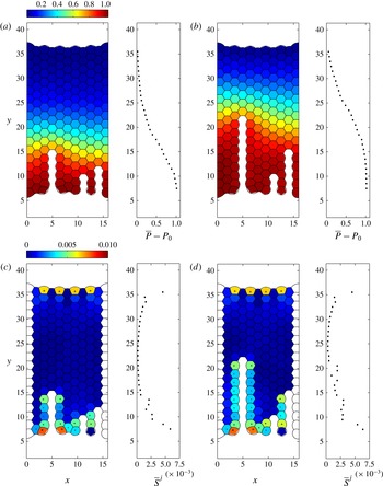
Figure 11. Gas pressure and maximal deviatoric stress for the brittle fracture example shown in figure 9. Colour maps of: (a) pressure distribution in the foam at point (a) of figure 10(a) (subtracting the baseline pressure
 $P_{0}$
); (b) pressure distribution at point (b) in figure 10(a) (subtracting the baseline pressure
$P_{0}$
); (b) pressure distribution at point (b) in figure 10(a) (subtracting the baseline pressure
 $P_{0}$
); (c,d) maximal deviatoric stress distributions at these same time points, respectively. In panels (c,d) the lines represent the magnitude and direction of the principal elastic stresses. To the right of each panel we further illustrate the distribution of the gas pressure (a,b) or maximal elastic stress (c,d) averaged over the
$P_{0}$
); (c,d) maximal deviatoric stress distributions at these same time points, respectively. In panels (c,d) the lines represent the magnitude and direction of the principal elastic stresses. To the right of each panel we further illustrate the distribution of the gas pressure (a,b) or maximal elastic stress (c,d) averaged over the
 $x$
coordinate, denoted with an overbar.
$x$
coordinate, denoted with an overbar.
Figure 11 further underlines the strongly localized character of the brittle crack tip. Figure 11(a,b) shows two snapshots of the entire foam (at the points labelled (a,b) in figure 10), with the bubble pressure distribution colour-coded, along with
 $x$
-averaged pressure profiles. As the primary crack advances, the increase in pressure is transmitted through the structure, with the transition between the initial pressure (
$x$
-averaged pressure profiles. As the primary crack advances, the increase in pressure is transmitted through the structure, with the transition between the initial pressure (
 ${\approx}P_{0}$
) and the driving pressure (
${\approx}P_{0}$
) and the driving pressure (
 $P_{0}+1$
) taking place in a narrow boundary layer (figure 11
a,b) of approximately five bubbles width. Note also how the pressure isolines tend to follow the regular lattice of the foam, indicating that microstructure is important for the details of this pressure wave transported at the speed of the brittle crack tip. This is a striking illustration and confirmation of the finding Arif et al. (Reference Arif, Tsai and Hilgenfeldt2010, Reference Arif, Tsai and Hilgenfeldt2012) that brittle cracks in foams are supersonic (cf. Guozden et al.
Reference Guozden, Jagla and Marder2010), outrunning relaxation of stress and pressure in the bulk of the foam and constantly re-establishing a localized stress distribution around their tips.
$P_{0}+1$
) taking place in a narrow boundary layer (figure 11
a,b) of approximately five bubbles width. Note also how the pressure isolines tend to follow the regular lattice of the foam, indicating that microstructure is important for the details of this pressure wave transported at the speed of the brittle crack tip. This is a striking illustration and confirmation of the finding Arif et al. (Reference Arif, Tsai and Hilgenfeldt2010, Reference Arif, Tsai and Hilgenfeldt2012) that brittle cracks in foams are supersonic (cf. Guozden et al.
Reference Guozden, Jagla and Marder2010), outrunning relaxation of stress and pressure in the bulk of the foam and constantly re-establishing a localized stress distribution around their tips.
By contrast, figure 11(c,d) illustrates, by a colour plot of the maximum deviatoric stress and its
 $x$
-averaged magnitude at the same time points, that bubble deformation caused by crack propagation is exclusively confined to the boundaries of the foam and of the newly generated crack. This confirms the brittle character of this type of material failure. A static signature of increased deviatoric stress can be seen towards the upstream boundary of the foam, but it remains unchanged until the brittle crack has reached that boundary, again confirming the supersonic character of propagation. It is interesting to note that, even far upstream of the crack tip, the aftermath of the passing crack leaves a significant amount of noise in the
$x$
-averaged magnitude at the same time points, that bubble deformation caused by crack propagation is exclusively confined to the boundaries of the foam and of the newly generated crack. This confirms the brittle character of this type of material failure. A static signature of increased deviatoric stress can be seen towards the upstream boundary of the foam, but it remains unchanged until the brittle crack has reached that boundary, again confirming the supersonic character of propagation. It is interesting to note that, even far upstream of the crack tip, the aftermath of the passing crack leaves a significant amount of noise in the
 $x$
-averaged deviatoric stress (correlated with the tips of secondary cracks, figure 11
c,d).
$x$
-averaged deviatoric stress (correlated with the tips of secondary cracks, figure 11
c,d).

Figure 12. Brittle fracture propagates by successive film rupture. (a–f) Six snapshots of the foam in the line of driving. (g) Pressure in the bubbles labelled A–C in (a) along the line of driving. (h) Perturbation dynamics in the films labelled (i)–(vi) in (a) in the line of driving; circles indicate points of rupture while dotted lines indicate the times of panels (a–f) at the instant before rupture occurs. (i) Pressure in the bubbles labelled D and E to the right of the main crack; note that the pressure spikes arising due to instantaneous rearrangement of the HPBs induce an increase in bubble pressure. (j) Perturbation growth in the film labelled (v) to the right of the main crack; this film does not rupture. Crosses in (a–f) indicate the position
 $x_{l}$
for each film in the plane
$x_{l}$
for each film in the plane
 $z=0$
.
$z=0$
.
The detailed simulation developed here gives further insight into the microscopic mechanism of successive film rupture by which the brittle crack elongates. In figure 12 we focus attention on a small region of the foam in and around the main brittle crack. Six snapshots of the propagation are shown in figure 12(a–f) at the six time points labelled with open circles in figure 12(h) (shown just before rupture occurs), while in figure 12(g) we plot the gas pressure in the three bubbles labelled A–C in the line of driving as a function of time and the corresponding temporal growth of the perturbation in the six rupturing films labelled (i)–(vi) (figure 12
h). It can be appreciated that the instabilities of successive films are proceeding simultaneously and reach the critical perturbation strength at regular time intervals that, when converted to dimensional quantities, are approximately
 $80~{\rm\mu}\text{s}$
, close to experimentally measured values (Arif et al.
Reference Arif, Tsai and Hilgenfeldt2010). Also in agreement with those experiments, the final, greatest increase of perturbation growth in a given film occurs after the film directly behind has ruptured (observe how the dotted lines indicating these ruptures in figure 12(h) occur simultaneously with the kinks in the curves indicating abruptly increased acceleration).
$80~{\rm\mu}\text{s}$
, close to experimentally measured values (Arif et al.
Reference Arif, Tsai and Hilgenfeldt2010). Also in agreement with those experiments, the final, greatest increase of perturbation growth in a given film occurs after the film directly behind has ruptured (observe how the dotted lines indicating these ruptures in figure 12(h) occur simultaneously with the kinks in the curves indicating abruptly increased acceleration).
Figure 12(i), by comparison, plots the gas pressures in the two bubbles labelled D and E to the right of the main crack, with the corresponding temporal growth of the perturbation in the film labelled (vii) between them shown in figure 12(j). The pressure in these bubbles shows characteristic peak signatures when the neighbouring bubbles suffer a film breakage and the fluid from the rupture rearranges. For example, the pressure in bubble D rises quickly once film (ii) has ruptured (figure 12 i), which drives a large acceleration of film (vii) (figure 12 j), causing the perturbation in this film to grow. However, the pressure difference is suppressed once film (iii) has ruptured, the perturbation in film (v) is damped out and the film remains intact. This intricate interplay of pressures and accelerations shows that the local environment of every bubble and every film is important for its fate during fracture.
5. Brittle fracture close to a microstructural defect
Our network model elucidates the role of microstructural elements in setting the direction and speed of foam fracture in a regular hexagonal array, in qualitative and semi-quantitative agreement with the experiments. Given the importance of the precise arrangement and orientation of the microstructure, our model can be further interrogated for the effects of irregularities in the foam. An important question of practical relevance is how propagating brittle cracks interact with structures of pre-existing disorder in the fracture path (Shilo et al. Reference Shilo, Sherman, Be’ery and Zolotoyabko2002; Sherman & Be’ery Reference Sherman and Be’ery2004). To this end, we introduce topological defects in the foam structure described in figure 5 by enforcing two T1 transitions in two non-neighbouring films directly ahead of the initial notch in the line of driving and then allow the system to find a new static equilibrium. The resulting structure has two dislocation defects (two pairs of bubbles with seven and five sides). Assuming that all the bubbles have an equal mass results in two very short HPBs in the new equilibrium, joining the seven- and six-sided bubbles. To overcome this effect, we increase (decrease) the mass in the seven-sided (five-sided) bubbles by 20 % and recompute the static configuration, shown in figure 13(a) along with the corresponding bubble pressure distribution (figure 13 b) and the maximal deviatoric stress in the foam (figure 13 c). Note that the presence of defects imposes significant static pressure differences in and around their locations, consistent with what can be expected from von Neumann’s law (von Neumann Reference von Neumann and Smith1952). They also lead to bubble deformations comparable to those near the initial notch (figure 13 c). The applied pressure differences of a brittle fracture are, however, much larger than these static imprints (cf. figure 12). Note that the maximal deviatoric stress in the pentagonal bubbles is quite small, as these smaller-volume bubbles with higher internal pressures can attain isotropic regular shapes: the pressure difference between the small bubble and any of its neighbours is typically larger than the pressure differences between the neighbours themselves.

Figure 13. Initial configuration for a pair of dislocation defects in the foam structure directly ahead of the line of driving for
 $P_{0}=100$
and
$P_{0}=100$
and
 ${\it\gamma}=0.0125$
. The mass of gas in the seven-sided (five-sided) bubbles has been increased (decreased) by 20 %: (a) initial structure of the foam; (b) colour plot of the global pressure distribution in the foam (subtracting the baseline pressure
${\it\gamma}=0.0125$
. The mass of gas in the seven-sided (five-sided) bubbles has been increased (decreased) by 20 %: (a) initial structure of the foam; (b) colour plot of the global pressure distribution in the foam (subtracting the baseline pressure
 $P_{0}$
); (c) colour plot of the maximum deviatoric stress in the foam.
$P_{0}$
); (c) colour plot of the maximum deviatoric stress in the foam.

Figure 14. Brittle fracture around a pair of dislocations for
 ${\it\gamma}=0.0125$
,
${\it\gamma}=0.0125$
,
 $P_{0}=100$
and
$P_{0}=100$
and
 $\mathscr{R}=2000$
using
$\mathscr{R}=2000$
using
 $K=4.94$
,
$K=4.94$
,
 $K_{l}=0.5$
and
$K_{l}=0.5$
and
 $K_{s}=15$
for pressure ramped linearly according to (4.1). (a–f) Six snapshots of the foam in the line of driving. (g) Pressure in the bubbles labelled A and D in (a). (h) Perturbation in the films labelled (i)–(v) in (a) (the sixth, unlabelled, trace corresponds to the film directly ahead of (v), not shown on panels (a–f)), where open circles and dotted lines indicate the times of panels (a–f) at the instant before rupture occurs. (i) Pressure in the bubbles labelled B and C in (a). (j) Perturbation in the films labelled (v) and (vi). Crosses in (a–f) indicate the position
$K_{s}=15$
for pressure ramped linearly according to (4.1). (a–f) Six snapshots of the foam in the line of driving. (g) Pressure in the bubbles labelled A and D in (a). (h) Perturbation in the films labelled (i)–(v) in (a) (the sixth, unlabelled, trace corresponds to the film directly ahead of (v), not shown on panels (a–f)), where open circles and dotted lines indicate the times of panels (a–f) at the instant before rupture occurs. (i) Pressure in the bubbles labelled B and C in (a). (j) Perturbation in the films labelled (v) and (vi). Crosses in (a–f) indicate the position
 $x_{l}$
for each film in the plane
$x_{l}$
for each film in the plane
 $z=0$
.
$z=0$
.
We consider brittle fracture of the initial defect configuration shown in figure 13(b) using the same ramping protocol (4.1) with
 $t_{R}=0.1$
. In figure 14 we illustrate six snapshots as the brittle crack propagates through the foam close to the defect at the six time points labelled with open circles in figure 14(h) (shown just before rupture occurs). The brittle fracture initiates as a straight line of film breakages in the direction of driving originating at the notch similar to figure 9 (figure 14
a). Upon encountering the first defect (film (i), figure 14
b), the crack has now reached a seven-sided bubble ahead with a lower gas pressure than all those around, so the crack propagates into this bubble and remains approximately straight (figure 14
b). In a similar manner, the crack propagates by rupturing film (ii) into the irregular hexagonal bubble directly ahead, between defects (figure 14
c). Next, the crack now encounters a five-sided bubble (second defect) directly ahead, which has a larger pressure than those in the bubbles to either side, so that the next film to rupture is not film (vi) directly ahead, but film (iii) adjoining the seven-sided bubble to the left of the crack tip, since this is the site of greatest pressure difference (figure 14
d). Upon engulfing this seven-sided bubble, the crack then propagates regularly forwards in a straight line of ruptures, with film breakage into the bubble directly ahead of the crack tip where the pressure difference across the film is greatest (figure 14
e,f, films (iv) and (v)). Slightly later, there is an additional side breakage of film (vii) to the right of the five-sided bubble as shown in figure 15(c). Similar side breakages are often observed in the experiments of Arif et al. (Reference Arif, Tsai and Hilgenfeldt2010). In figure 14(g) we plot the pressures in the bubbles labelled A and D in figure 14(a), while figure 14(h) depicts the corresponding growth of the perturbation in each of the films (i)–(v) in figure 14(a). Also, in figure 14(i) we plot the pressures in the bubbles labelled B and C in figure 14(a), while figure 14(j) depicts the corresponding growth of the perturbation in the films labelled (vi) and (vii) in figure 14(a). Notably, film (vi) undergoes instability almost in parallel with film (iii), but its perturbation amplitude is reset through the fluid rearrangement after the rupture of film (iii) and never gets close to rupture again. It is noteworthy that the distribution of deviatoric stress in the initial structure (figure 13
c) prefigures the deviation of the crack path. Selective localized displacements of brittle cracks encountering defects have been described in experimental metal fracture from fracture surface data (Shilo et al.
Reference Shilo, Sherman, Be’ery and Zolotoyabko2002; Sherman & Be’ery Reference Sherman and Be’ery2004); in our model, the microscopic details of the analogous process can be studied.
$t_{R}=0.1$
. In figure 14 we illustrate six snapshots as the brittle crack propagates through the foam close to the defect at the six time points labelled with open circles in figure 14(h) (shown just before rupture occurs). The brittle fracture initiates as a straight line of film breakages in the direction of driving originating at the notch similar to figure 9 (figure 14
a). Upon encountering the first defect (film (i), figure 14
b), the crack has now reached a seven-sided bubble ahead with a lower gas pressure than all those around, so the crack propagates into this bubble and remains approximately straight (figure 14
b). In a similar manner, the crack propagates by rupturing film (ii) into the irregular hexagonal bubble directly ahead, between defects (figure 14
c). Next, the crack now encounters a five-sided bubble (second defect) directly ahead, which has a larger pressure than those in the bubbles to either side, so that the next film to rupture is not film (vi) directly ahead, but film (iii) adjoining the seven-sided bubble to the left of the crack tip, since this is the site of greatest pressure difference (figure 14
d). Upon engulfing this seven-sided bubble, the crack then propagates regularly forwards in a straight line of ruptures, with film breakage into the bubble directly ahead of the crack tip where the pressure difference across the film is greatest (figure 14
e,f, films (iv) and (v)). Slightly later, there is an additional side breakage of film (vii) to the right of the five-sided bubble as shown in figure 15(c). Similar side breakages are often observed in the experiments of Arif et al. (Reference Arif, Tsai and Hilgenfeldt2010). In figure 14(g) we plot the pressures in the bubbles labelled A and D in figure 14(a), while figure 14(h) depicts the corresponding growth of the perturbation in each of the films (i)–(v) in figure 14(a). Also, in figure 14(i) we plot the pressures in the bubbles labelled B and C in figure 14(a), while figure 14(j) depicts the corresponding growth of the perturbation in the films labelled (vi) and (vii) in figure 14(a). Notably, film (vi) undergoes instability almost in parallel with film (iii), but its perturbation amplitude is reset through the fluid rearrangement after the rupture of film (iii) and never gets close to rupture again. It is noteworthy that the distribution of deviatoric stress in the initial structure (figure 13
c) prefigures the deviation of the crack path. Selective localized displacements of brittle cracks encountering defects have been described in experimental metal fracture from fracture surface data (Shilo et al.
Reference Shilo, Sherman, Be’ery and Zolotoyabko2002; Sherman & Be’ery Reference Sherman and Be’ery2004); in our model, the microscopic details of the analogous process can be studied.

Figure 15. Snapshots of the gas pressure distribution in the defective foam structure with two dislocations (subtracting the baseline pressure
 $P_{0}$
). All parameters are as in figure 14. The same overall pattern of pressure in brittle fracture as for a regular foam persists, but shifts position by one bubble width upon encountering the defects.
$P_{0}$
). All parameters are as in figure 14. The same overall pattern of pressure in brittle fracture as for a regular foam persists, but shifts position by one bubble width upon encountering the defects.
Examining the global pressure distribution across the foam as the crack propagates through the defective region, we see in figure 15 that the localized drop-off of pressure in front of the crack tip persists as in the case of the regular foam, including the orientation of the pressure isolines along the main symmetry lines of the foam. However, the entire pressure pattern shifts with the position change of the crack tip. Thus, encounters of the fracture with this type of defect influence crack propagation (and can lead to a minimal retardation of effective speed in the
 $y$
direction), but are not prone to change the overall pattern of fracture.
$y$
direction), but are not prone to change the overall pattern of fracture.
6. Discussion
We have constructed a large-scale network model to explore the fracture of an aqueous foam monolayer by an applied driving pressure. Asymptotic ordinary differential equation models were developed for the dynamics of each liquid structure in the foam, i.e. the horizontal and vertical Plateau borders and their intersection at Plateau border nodes as well as the liquid lamellae spanning between the plates. These reduced models are coupled to an ideal gas law in the bubbles and constraints on T1 transitions when any two PBNs come within a fixed distance, in addition to scaling laws for the growth of Raleigh–Taylor instability in the liquid lamellae as they are accelerated forwards. This model exploits the observation that for low liquid fractions the HPBs and VPBs are typically long and thin. For slow non-inertial motion, a reduced model is used for the PBN to simplify and save computational effort, neglecting the interfacial curvature in the out-of-plane direction.
It should be stressed that the model includes descriptions of physical phenomena on many different length and time scales, from the microseconds of film instability to the seconds of pressure ramping and ductile crack propagation. The modular approach, and the advantages of combining integral properties into geometrically simplified elements, leads to an efficient multiscale formalism that allows for exploration of the rich behaviour observed in experiment, but without the limitations to experimental microstructure preparation.
The model is successful in reproducing and quantifying the two experimentally observed modes of fracture, selected depending on the rate of applied stress (the rise time of applied pressure). When the pressure driving is applied slowly, our model predicts the propagation of a crack via a ductile fracture, where the void enlarges by successive T1 transitions as bubbles surrounding the crack interchange neighbours (figure 6). When viewed at length scales much larger than the size of individual bubbles, this mode of propagation can be understood as a fingering instability (Saffman Reference Saffman1986; Zocchi et al. Reference Zocchi, Shaw, Libchaber and Kadanoff1987) in a viscoelastic medium (Ro & Homsy Reference Ro and Homsy1995; Ben-Amar & Poire Reference Ben-Amar and Poire1999). Similar dynamics are also exhibited as a large single bubble propagates through a monodisperse foam (Cantat & Delannay Reference Cantat and Delannay2003, Reference Cantat and Delannay2005). The present model, however, allows for detailed tracking of the deformations and displacements of individual bubbles, and thus for an evaluation of the role of the microstructural make-up of the foam. It therefore gives access to a novel type of fingering study in media with discrete domain structure.
The developing ductile crack settles into a finger with a width that is a finite fraction of the channel width, and displays a propagation speed consistent with the experiments of Hilgenfeldt et al. (Reference Hilgenfeldt, Arif and Tsai2008) when using comparable parameters to those experiments. The model also shows rapid development of the expected linear pressure profile in the entire foam in front of the crack tip. Beyond such foam-scale measures, the simulations yield detailed information on the geometry of individual bubbles and the inferred stress on the bubbles. We demonstrate that T1 transitions in which bubbles participate, as well as other T1 transitions nearby, leave distinctive traces in the stress and strain of the bubbles, superimposed on the longer-time dynamics as the bubble repositions itself relative to the passing crack tip.
By contrast, when the pressure driving is applied rapidly, our model instead predicts the propagation of a crack by a brittle fracture, where the void enlarges by successive rupture of liquid films in a line parallel to the applied pressure gradient (figure 9). The simulations show a well-defined localized stress concentration at the tip of this crack that stably propagates at a speed much higher than that of the ductile fracture. This speed is again consistent with that observed in experiment (Arif et al.
Reference Arif, Tsai and Hilgenfeldt2010, Reference Arif, Tsai and Hilgenfeldt2012), while the pressure in front of the crack tip now drops to the ambient pressure within a thin layer forwards of the crack tip (this layer has a width of a few bubble lengths). This shows that, as was postulated in (Arif et al.
Reference Arif, Tsai and Hilgenfeldt2010, Reference Arif, Tsai and Hilgenfeldt2012), the stress field does not propagate through the entire foam, but is slaved to the dynamics of the crack tip, where a Rayleigh–Taylor instability sets the time scale of successive film breakage, and thus of fracture speed. The deviatoric stress in bubbles around the propagating brittle crack is very localized (in keeping with the fracture characterization as brittle), and the brittle crack settles very quickly into a consistent, constant-speed propagation. Deformation signals do not propagate into the bulk of the foam ahead of the crack, and the fracture can therefore be termed supersonic. This model could potentially be used to elucidate the mechanisms of brittle-to-ductile transition (observed in the experiments of Arif et al. (Reference Arif, Tsai and Hilgenfeldt2012)) by systematically changing
 $t_{R}$
, but this will be left for future study.
$t_{R}$
, but this will be left for future study.
Given the extreme localization of stress in the brittle mode, and the high selectivity with which the next film to break is determined as the film straight ahead of the current crack tip, it is natural to ask for modifications in the crack propagation caused by frozen defects in the initial foam structure. Our model allows for versatile exploration of this question, and we have shown here that dislocation defects indeed deflect the crack tip (consistent with experiments), as the static pressure variations around the defect are sufficient to alter the sequence of film breakages from that in a completely ordered foam. The film straight ahead of the fracture tip is now not necessarily the most unstable one, as the crack preferentially seeks passage through bubbles with a larger number of neighbours, which possess lower static pressure. The result is a displacement of the crack tip, with no lasting or larger-scale disturbance of the propagation mode or the accompanying pressure field, which quickly readjust. The versatility and generality of our model allows for a detailed discussion of the role of microstructure and defects in brittle and ductile fracture, which will be the focus of a future publication, including a systematic study of defect orientation and density. In addition, this model allows examination of the role of interfacial boundary conditions in the propagation and suppression of fracture, as investigated experimentally by Ben Salem, Cantat & Dollet (Reference Ben Salem, Cantat and Dollet2013a ) in a slightly different geometry, where they found that incompressible interfaces result in significantly slower propagation and fracture of the foam compared to mobile interfaces. Such studies will be of use not just as a general model system for crack propagation in heterogeneous media, but directly for applications where film breakage and fracture of foam are crucial phenomena, such as foam flotation or secondary oil recovery.
Acknowledgements
Funding from NSF grant no. CMMI-0826703 is very gratefully acknowledged (P.S.S. and S.H.D.). The authors would also like to thank the anonymous referees for their very helpful comments.
Appendix A. Plateau border nodes
Consider a PBN on the wall of the domain (
 $M=2$
,
$M=2$
,
 $N=3$
, as shown in figure 3
c). We assume that the outer shape of the PBN can be approximated as half of a square pyramid of side length
$N=3$
, as shown in figure 3
c). We assume that the outer shape of the PBN can be approximated as half of a square pyramid of side length
 $\overline{a}_{p}$
, height
$\overline{a}_{p}$
, height
 $H=\overline{a}_{p}/\sqrt{2}$
and volume
$H=\overline{a}_{p}/\sqrt{2}$
and volume
 $V_{p}=1/(6\sqrt{2})\overline{a}_{p}^{3}$
.
$V_{p}=1/(6\sqrt{2})\overline{a}_{p}^{3}$
.
Having determined the height and volume, we now turn to computing the forces. In the plane of the plate we enforce that each pair of gas–liquid interfaces must meet tangentially at the same point along the tangent to the adjoining HPB (see PBN cross-section in figure 3 d).
For simplicity (and tractability), we neglect the interfacial curvature in the out-of-plane direction and assume that in each horizontal cross-section of the PBN the two gas–liquid interfaces have constant radius of curvature
 $a_{pm}$
(
$a_{pm}$
(
 $m=1,\ldots ,M$
) that varies linearly in the
$m=1,\ldots ,M$
) that varies linearly in the
 $z$
coordinate. This assumption facilitates a simple method to estimate the coefficient of the restoring force on the PBN due to surface tension. However, this assumption has no influence on the additional terms that arise in the force model below (see (A 5) and (A 6)) that must be neglected to prevent violation of Plateau’s laws when the foam is in static equilibrium. Since the interface is uniformly sloped in the
$z$
coordinate. This assumption facilitates a simple method to estimate the coefficient of the restoring force on the PBN due to surface tension. However, this assumption has no influence on the additional terms that arise in the force model below (see (A 5) and (A 6)) that must be neglected to prevent violation of Plateau’s laws when the foam is in static equilibrium. Since the interface is uniformly sloped in the
 $z$
direction, we calculate the corresponding angle of inclination
$z$
direction, we calculate the corresponding angle of inclination
 ${\it\theta}$
of the tetrahedral interface relative to the
${\it\theta}$
of the tetrahedral interface relative to the
 $z$
axis. For the PBN on the lower plate (
$z$
axis. For the PBN on the lower plate (
 $z=-b/2$
) this takes the form
$z=-b/2$
) this takes the form
 $\cos {\it\theta}=\sin {\it\theta}=1/\sqrt{2}$
. In each cross-section we parametrize the circular arc of interface
$\cos {\it\theta}=\sin {\it\theta}=1/\sqrt{2}$
. In each cross-section we parametrize the circular arc of interface
 $m$
using the coordinate
$m$
using the coordinate
 ${\it\phi}_{m}$
such that
${\it\phi}_{m}$
such that
 ${\it\phi}_{m1}\leqslant {\it\phi}_{m}\leqslant {\it\phi}_{m2}$
(
${\it\phi}_{m1}\leqslant {\it\phi}_{m}\leqslant {\it\phi}_{m2}$
(
 $m=1,\ldots ,M$
), where
$m=1,\ldots ,M$
), where
 ${\it\phi}_{m}=0$
is along the
${\it\phi}_{m}=0$
is along the
 $x$
axis, so that the curvature radius of each gas–liquid interface takes the form
$x$
axis, so that the curvature radius of each gas–liquid interface takes the form
 $$\begin{eqnarray}\displaystyle & & \displaystyle a_{pm}=\overline{a}_{p}\cos {\it\theta}\tan \left(\frac{1}{2}({\it\phi}_{m2}-{\it\phi}_{m1})\right)\frac{H-{\textstyle \frac{1}{2}}b-z}{H},\nonumber\\ \displaystyle & & \displaystyle \quad \left(m=1,\ldots ,M,-\frac{1}{2}b\leqslant z\leqslant H-\frac{1}{2}b\right).\end{eqnarray}$$
The corresponding outward-pointing unit normal to each interface takes the form
 $$\begin{eqnarray}\hat{\boldsymbol{n}}_{pm}=(\cos {\it\phi}_{m}\cos {\it\theta},\sin {\it\phi}_{m}\cos {\it\theta},\sin {\it\theta})\quad (m=1,\ldots ,M).\end{eqnarray}$$
We consider the pressure on each gas–liquid interface (2.3e
), which assuming
 ${\it\gamma}\gg \mathscr{R}^{-1}$
is well approximated by
${\it\gamma}\gg \mathscr{R}^{-1}$
is well approximated by
 $$\begin{eqnarray}p_{m}=P_{m}-\frac{{\it\gamma}}{a_{pm}}\quad (m=1,\ldots ,M).\end{eqnarray}$$
Integrating, we obtain the total force exerted on the gas–liquid interface. For a PBN on the lower plate (
 $z=-b/2$
) this takes the form
$z=-b/2$
) this takes the form
 $$\begin{eqnarray}\tilde{\boldsymbol{F}}_{pm}=\int _{{\it\phi}_{m1}}^{{\it\phi}_{m2}}\int _{-b/2}^{H-b/2}\left(P_{m}-\frac{{\it\gamma}}{a_{pm}}\right)\hat{\boldsymbol{n}}_{pm}a_{pm}\,\text{d}z\,\text{d}{\it\phi}_{m}\quad (m=1,\ldots ,M).\end{eqnarray}$$
Since the PBN always remains attached to the plates, we ignore the component in the
 $\hat{\boldsymbol{z}}$
direction (and drop the tilde), and so denote the planar component of this force as
$\hat{\boldsymbol{z}}$
direction (and drop the tilde), and so denote the planar component of this force as
 $\boldsymbol{F}_{pm}$
(
$\boldsymbol{F}_{pm}$
(
 $m=1,\ldots ,M$
).
$m=1,\ldots ,M$
).
In this case it emerges that we can express
 ${\it\phi}_{m2}$
and
${\it\phi}_{m2}$
and
 ${\it\phi}_{m1}$
(
${\it\phi}_{m1}$
(
 $m=1,2$
) in terms of the deflection of the adjoining HPB from the
$m=1,2$
) in terms of the deflection of the adjoining HPB from the
 $\hat{\boldsymbol{x}}$
direction, denoted by
$\hat{\boldsymbol{x}}$
direction, denoted by
 ${\it\alpha}$
in figure 3(d), where
${\it\alpha}$
in figure 3(d), where
 ${\it\alpha}>0$
corresponds to a PBN that is deflected in the positive
${\it\alpha}>0$
corresponds to a PBN that is deflected in the positive
 $y$
direction. For example for a PBN on the sidewall at
$y$
direction. For example for a PBN on the sidewall at
 $x=0$
, as in figure 3(b,d), we can express
$x=0$
, as in figure 3(b,d), we can express
 ${\it\phi}_{11}={\rm\pi}/2+{\it\alpha}$
,
${\it\phi}_{11}={\rm\pi}/2+{\it\alpha}$
,
 ${\it\phi}_{12}={\rm\pi}$
,
${\it\phi}_{12}={\rm\pi}$
,
 ${\it\phi}_{21}={\rm\pi}$
and
${\it\phi}_{21}={\rm\pi}$
and
 ${\it\phi}_{22}=3{\rm\pi}/2+{\it\alpha}$
. The total force on the PBN in the direction along
${\it\phi}_{22}=3{\rm\pi}/2+{\it\alpha}$
. The total force on the PBN in the direction along
 $y$
is
$y$
is
 $$\begin{eqnarray}\hat{\boldsymbol{y}}\boldsymbol{\cdot }\mathop{\sum }_{m=1}^{2}\boldsymbol{F}_{pm}=\frac{\overline{a}_{p}^{2}}{4\sqrt{2}}\frac{(P_{1}-P_{2})}{\cos {\it\alpha}}+\overline{a}_{p}{\it\gamma}\sin {\it\alpha}.\end{eqnarray}$$
The first term on the right-hand side of (A 5) involves the net pressure difference between the bubbles on either side of the HPB. However, retaining this term violates Plateau’s law in the initial static equilibrium: the HPBs joining to the wall are no longer perpendicular to the wall, especially at the upstream and downstream ends of the foam, where there are appreciable pressure differences between bubbles. Hence, for consistency in this network model formulation, we formally neglect terms of
 $O(\overline{a}_{p}^{2})$
to obtain the force model (3.3a
) at leading order. The neglect of this term is discussed further below (A 6).
$O(\overline{a}_{p}^{2})$
to obtain the force model (3.3a
) at leading order. The neglect of this term is discussed further below (A 6).
Analogously, we consider a trijunction PBN (
 $M=3$
,
$M=3$
,
 $N=3$
) as described in § 3.1 and depicted in figure 4(a,b). In this case the outer shape of the PBN is approximated as a regular tetrahedron of side length
$N=3$
) as described in § 3.1 and depicted in figure 4(a,b). In this case the outer shape of the PBN is approximated as a regular tetrahedron of side length
 $\overline{a}_{p}$
and height
$\overline{a}_{p}$
and height
 $H=\sqrt{2/3}\,\overline{a}_{p}$
with corresponding volume
$H=\sqrt{2/3}\,\overline{a}_{p}$
with corresponding volume
 $V_{p}=1/(6\sqrt{2})\overline{a}_{p}^{3}$
(figure 3
a). We again neglect the interfacial curvature in the out-of-plane direction and enforce that each pair of gas–liquid interfaces must meet tangentially at the same point along the tangent to the adjoining HPB (see cross-section in figure 3
b). We parametrize each circular arc of interface
$V_{p}=1/(6\sqrt{2})\overline{a}_{p}^{3}$
(figure 3
a). We again neglect the interfacial curvature in the out-of-plane direction and enforce that each pair of gas–liquid interfaces must meet tangentially at the same point along the tangent to the adjoining HPB (see cross-section in figure 3
b). We parametrize each circular arc of interface
 $m$
(in the plane of the plates) using the coordinate
$m$
(in the plane of the plates) using the coordinate
 ${\it\phi}_{m}$
such that
${\it\phi}_{m}$
such that
 ${\it\phi}_{m1}\leqslant {\it\phi}_{m}\leqslant {\it\phi}_{m2}$
 $(m=1,\ldots ,M)$
, so that the radius of curvature of each interface is given by (A 1) and the corresponding outward-pointing normal by (A 2). In this case the corresponding angle of inclination
$(m=1,\ldots ,M)$
, so that the radius of curvature of each interface is given by (A 1) and the corresponding outward-pointing normal by (A 2). In this case the corresponding angle of inclination
 ${\it\theta}$
of the tetrahedral interface relative to the
${\it\theta}$
of the tetrahedral interface relative to the
 $z$
axis fulfills
$z$
axis fulfills
 $\cos {\it\theta}=\sqrt{2}/\sqrt{3}$
and
$\cos {\it\theta}=\sqrt{2}/\sqrt{3}$
and
 $\sin {\it\theta}=1/\sqrt{3}$
.
$\sin {\it\theta}=1/\sqrt{3}$
.
The pressure on each gas–liquid interface is given by (A 3), so the total force on each interface in the plane of the plates is given by
 $$\begin{eqnarray}\displaystyle \boldsymbol{F}_{pm}=\frac{2\overline{a}_{p}}{3}\left(\frac{a_{pm}}{2\sqrt{3}}P_{m}-{\it\gamma}\right)[\hat{\boldsymbol{x}}\sin {\it\phi}_{m}-\hat{\boldsymbol{y}}\cos {\it\phi}_{m}]_{{\it\phi}_{m1}}^{{\it\phi}_{m2}}\quad (m=1,\ldots ,M). & & \displaystyle\end{eqnarray}$$
However, as in (A 5), this force contains a contribution from a term reflecting the net pressure difference between the adjacent bubbles, which must be neglected for the force balance to be consistent with Plateau’s law, resulting in the force term (3.2a ). This additional term also appears in the entirely two-dimensional system of Cantat (Reference Cantat2013) and is not a consequence of our assumption of linear variation of the PBN curvature in the out-of-plane direction. Neglecting this component seems reasonable in the ductile regime reported in § 4.2, but in the brittle regime this extra term could be significant around the tip of the crack. To confirm that its neglect is reasonable, we have repeated the simulations reported in § 4.3 while including this extra term and have found that its inclusion results in no qualitative and little quantitative difference to the behaviour. We are therefore satisfied that neglecting this contribution to the driving force is not influencing our results significantly.
In addition, there are two contributions to the viscous drag on the PBN as it moves. Most importantly, there is a drag force due to the precursor liquid layer on the plates which originates from the matching region between the PBN and the liquid film on the plate. The viscous shear force per unit length for a spatially extended PBN moving at speed
 $U$
can be written in the compact form
$U$
can be written in the compact form
 $$\begin{eqnarray}K\frac{{\it\gamma}^{1/3}}{\mathscr{R}^{2/3}}U^{2/3},\end{eqnarray}$$
where
 $K$
is an
$K$
is an
 $O(1)$
constant that depends on the tangential stress condition on the gas–liquid interface. In the very viscous limit this constant can be calculated explicitly: for example, imposing no-tangential stress on the interfaces results in
$O(1)$
constant that depends on the tangential stress condition on the gas–liquid interface. In the very viscous limit this constant can be calculated explicitly: for example, imposing no-tangential stress on the interfaces results in
 $K=4.94$
(Cantat Reference Cantat2013). For simplicity, we assume that this form of the drag term also applies to our finite PBN structures, where we approximate the total viscous drag as it moves across the plates using (A 7) integrated around the outer perimeter of the PBN in contact with the liquid layer on the plate. We recognize that the constant
$K=4.94$
(Cantat Reference Cantat2013). For simplicity, we assume that this form of the drag term also applies to our finite PBN structures, where we approximate the total viscous drag as it moves across the plates using (A 7) integrated around the outer perimeter of the PBN in contact with the liquid layer on the plate. We recognize that the constant
 $K$
may vary depending on the geometry between sidewall PBN (
$K$
may vary depending on the geometry between sidewall PBN (
 $M=2$
,
$M=2$
,
 $N=3$
) and a trijunction PBN (
$N=3$
) and a trijunction PBN (
 $M=3$
,
$M=3$
,
 $N=3$
), as well as on the local surfactant concentration, but for simplicity in the simulations reported in § 4 we assume
$N=3$
), as well as on the local surfactant concentration, but for simplicity in the simulations reported in § 4 we assume
 $K=4.94$
across all the PBN structures (and indeed the HPBs discussed in appendix B below). There is an additional drag force due to internal viscous dissipation in the node, but this contribution is
$K=4.94$
across all the PBN structures (and indeed the HPBs discussed in appendix B below). There is an additional drag force due to internal viscous dissipation in the node, but this contribution is
 $O(\mathscr{R}^{-1})$
(recall
$O(\mathscr{R}^{-1})$
(recall
 $\mathscr{R}=2000$
in experiments) and can be neglected in comparison to (A 7).
$\mathscr{R}=2000$
in experiments) and can be neglected in comparison to (A 7).
Appendix B. Horizontal Plateau borders
Consider the HPB of volume
 $V_{h}$
discussed in § 3.1 and shown in figure 4(a), where the two HPB gas–liquid interfaces (indexed with
$V_{h}$
discussed in § 3.1 and shown in figure 4(a), where the two HPB gas–liquid interfaces (indexed with
 $m=1,2$
) are uniformly curved in both directions (see cross-sections in figure 4
b,c). When the adjoining liquid lamella is perpendicular to the plates, these interfaces have constant radius of curvature
$m=1,2$
) are uniformly curved in both directions (see cross-sections in figure 4
b,c). When the adjoining liquid lamella is perpendicular to the plates, these interfaces have constant radius of curvature
 $\overline{a}_{h}$
. In general, we parametrize each gas–liquid interface using polar coordinates with constant radius
$\overline{a}_{h}$
. In general, we parametrize each gas–liquid interface using polar coordinates with constant radius
 $1/|{\it\kappa}_{h}|$
and angle
$1/|{\it\kappa}_{h}|$
and angle
 ${\it\phi}_{m}$
in the plane of the plate (
${\it\phi}_{m}$
in the plane of the plate (
 ${\it\phi}_{m1}\leqslant {\it\phi}_{m}\leqslant {\it\phi}_{m2}$
, where
${\it\phi}_{m1}\leqslant {\it\phi}_{m}\leqslant {\it\phi}_{m2}$
, where
 ${\it\phi}_{m}$
is measured anticlockwise relative to the
${\it\phi}_{m}$
is measured anticlockwise relative to the
 $x$
axis,
$x$
axis,
 $m=1,2$
), and constant radius
$m=1,2$
), and constant radius
 $a_{hm}$
and angle
$a_{hm}$
and angle
 ${\it\theta}_{m}$
in the plane normal to the plate (
${\it\theta}_{m}$
in the plane normal to the plate (
 ${\it\theta}_{m1}\leqslant {\it\theta}_{m}\leqslant {\it\theta}_{m2}$
, where
${\it\theta}_{m1}\leqslant {\it\theta}_{m}\leqslant {\it\theta}_{m2}$
, where
 ${\it\theta}_{m}$
is measured anticlockwise from the
${\it\theta}_{m}$
is measured anticlockwise from the
 $z$
axis,
$z$
axis,
 $m=1,2$
). To leading order, the curvatures of the interfaces in the plane of the plate must be identical, denoted
$m=1,2$
). To leading order, the curvatures of the interfaces in the plane of the plate must be identical, denoted
 ${\it\kappa}_{h}(t)$
and defined in (3.5), while the curvatures of these HPB interfaces in the out-of-plane direction are denoted
${\it\kappa}_{h}(t)$
and defined in (3.5), while the curvatures of these HPB interfaces in the out-of-plane direction are denoted
 $a_{hm}$
(
$a_{hm}$
(
 $m=1,2$
), where
$m=1,2$
), where
 $$\begin{eqnarray}a_{hm}=\overline{a}_{h}\tan ({\textstyle \frac{1}{2}}{\rm\pi}-{\textstyle \frac{1}{2}}({\it\theta}_{m2}-{\it\theta}_{m1}))\quad (m=1,2).\end{eqnarray}$$
When the attached film is perpendicular to the plates,
 $a_{h1}=a_{h2}=\overline{a}_{h}$
. The corresponding normal to interface
$a_{h1}=a_{h2}=\overline{a}_{h}$
. The corresponding normal to interface
 $m$
takes the form
$m$
takes the form
 $$\begin{eqnarray}\hat{\boldsymbol{n}}_{hm}({\it\theta}_{m},{\it\phi}_{m})=(\cos {\it\phi}_{m}\sin {\it\theta}_{m},\sin {\it\phi}_{m}\sin {\it\theta}_{m},\cos {\it\theta}_{m})\quad (m=1,2).\end{eqnarray}$$
For
 ${\it\gamma}\gg \mathscr{R}^{-1}$
, the liquid pressure on each interface follows from the normal stress condition (2.3e
), in the form
${\it\gamma}\gg \mathscr{R}^{-1}$
, the liquid pressure on each interface follows from the normal stress condition (2.3e
), in the form
 $$\begin{eqnarray}p_{m}=P_{m}-{\it\gamma}\left(\frac{1}{a_{hm}}+{\it\kappa}_{h}\right)\quad (m=1,2),\end{eqnarray}$$
where we have enforced that the gas–liquid interfaces intersect on the tangent to the HPB as it passes through the PBN (see figure 4). We compute the force exerted across each HPB interface by integrating over the gas–liquid interface,
 $$\begin{eqnarray}\tilde{\boldsymbol{F}}_{hm}=\int _{{\it\phi}_{m1}}^{{\it\phi}_{m2}}\int _{{\it\theta}_{m1}}^{{\it\theta}_{m2}}\left(P_{m}-{\it\gamma}\left(\frac{1}{a_{hm}}+{\it\kappa}_{h}\right)\right)\hat{\boldsymbol{n}}_{hm}\frac{a_{hm}}{|{\it\kappa}_{h}|}\,\text{d}{\it\theta}_{m}\,\text{d}{\it\phi}_{m}\quad (m=1,2).\end{eqnarray}$$
Denoting the deflection of the tangent to the adjoining lamella as the angle
 ${\it\beta}$
(where
${\it\beta}$
(where
 ${\it\beta}>0$
represents a deflection in the positive
${\it\beta}>0$
represents a deflection in the positive
 $x_{h}$
direction), the angles
$x_{h}$
direction), the angles
 ${\it\phi}_{m1}$
and
${\it\phi}_{m1}$
and
 ${\it\phi}_{m2}$
can then be expressed in terms of
${\it\phi}_{m2}$
can then be expressed in terms of
 ${\it\beta}$
. For example, for the HPB shown in figure 4(b), we can express
${\it\beta}$
. For example, for the HPB shown in figure 4(b), we can express
 ${\it\theta}_{11}={\rm\pi}$
,
${\it\theta}_{11}={\rm\pi}$
,
 ${\it\theta}_{12}=3{\rm\pi}/2-{\it\beta}$
,
${\it\theta}_{12}=3{\rm\pi}/2-{\it\beta}$
,
 ${\it\theta}_{21}={\rm\pi}/2-{\it\beta}$
and
${\it\theta}_{21}={\rm\pi}/2-{\it\beta}$
and
 ${\it\theta}_{22}={\rm\pi}$
. Hence, we obtain the total driving force on the HPB (neglecting the component in the
${\it\theta}_{22}={\rm\pi}$
. Hence, we obtain the total driving force on the HPB (neglecting the component in the
 $\hat{\boldsymbol{z}}$
direction and dropping the tilde) in terms of
$\hat{\boldsymbol{z}}$
direction and dropping the tilde) in terms of
 ${\it\beta}$
(substituting (B 1)) as
${\it\beta}$
(substituting (B 1)) as
 $$\begin{eqnarray}\mathop{\sum }_{m=1}^{2}\boldsymbol{F}_{hm}=L_{h}\left(\overline{a}_{h}\frac{({\rm\Delta}P_{l}-2{\it\gamma}{\it\kappa}_{h})}{\cos {\it\beta}}+2{\it\gamma}\sin {\it\beta}\right)\hat{\boldsymbol{n}}_{h},\end{eqnarray}$$
where
 ${\rm\Delta}P_{l}=P_{1}-P_{2}$
.
${\rm\Delta}P_{l}=P_{1}-P_{2}$
.
In the ductile regime, we assume that the film does not bend significantly in the out-of-plane direction (
 ${\it\beta}=0$
) and the net force on HPB is uniformly zero, so we can compute the HPB curvature from (3.6) obtained by enforcing that (B 5) is identically zero. Conversely, in the brittle regime, we conduct a force balance about the geometric centre of the HPB (denoted
${\it\beta}=0$
) and the net force on HPB is uniformly zero, so we can compute the HPB curvature from (3.6) obtained by enforcing that (B 5) is identically zero. Conversely, in the brittle regime, we conduct a force balance about the geometric centre of the HPB (denoted
 $\boldsymbol{x}_{h}$
). The drag force per unit length takes a form identical to (A 7) as derived by Cantat (Reference Cantat2013), so the balance of linear momentum on the HPB takes the approximate form
$\boldsymbol{x}_{h}$
). The drag force per unit length takes a form identical to (A 7) as derived by Cantat (Reference Cantat2013), so the balance of linear momentum on the HPB takes the approximate form
 $$\begin{eqnarray}\frac{\text{d}}{\text{d}t}\left(V_{h}\frac{\text{d}\boldsymbol{x}_{h}}{\text{d}t}\right)=L_{h}\left(\overline{a}_{h}\frac{({\rm\Delta}P_{l}-2{\it\gamma}{\it\kappa}_{h})}{\cos {\it\beta}}+2{\it\gamma}\sin {\it\beta}\right)\hat{\boldsymbol{n}}_{h}-L_{h}K\frac{{\it\gamma}^{1/3}}{\mathscr{R}^{2/3}}\hat{\boldsymbol{e}}_{h}\left|\frac{\text{d}\boldsymbol{x}_{h}}{\text{d}t}\right|^{2/3},\end{eqnarray}$$
where
 $\hat{\boldsymbol{e}}_{h}$
is a unit vector in the direction of
$\hat{\boldsymbol{e}}_{h}$
is a unit vector in the direction of
 $\dot{\boldsymbol{x}}_{h}$
. Taking the component of (B 6) in the direction of
$\dot{\boldsymbol{x}}_{h}$
. Taking the component of (B 6) in the direction of
 $\hat{\boldsymbol{n}}_{h}$
(the unit normal to the HPB midline introduced in § 3.2), we obtain a scalar governing equation for the deflection of the HPB midline in the form (3.7). Note that in this model we neglect the time dependence of the unit normal
$\hat{\boldsymbol{n}}_{h}$
(the unit normal to the HPB midline introduced in § 3.2), we obtain a scalar governing equation for the deflection of the HPB midline in the form (3.7). Note that in this model we neglect the time dependence of the unit normal
 $\hat{\boldsymbol{n}}_{h}$
.
$\hat{\boldsymbol{n}}_{h}$
.
Note that, if the HPB equation (B 6) is dominated by the balance between the capillary term
 $2L_{h}{\it\gamma}\sin ({\it\beta})$
and the drag term, and likewise if the film out-of-plane motion (3.8a
) is dominated by the Young–Laplace term
$2L_{h}{\it\gamma}\sin ({\it\beta})$
and the drag term, and likewise if the film out-of-plane motion (3.8a
) is dominated by the Young–Laplace term
 ${\rm\Delta}P_{l}=2{\it\gamma}({\it\kappa}_{h}+{\it\kappa}_{p})$
, then it is possible to derive a version of the viscous froth model (Grassia et al.
Reference Grassia, Montes-Atenas, Lue and Green2008).
${\rm\Delta}P_{l}=2{\it\gamma}({\it\kappa}_{h}+{\it\kappa}_{p})$
, then it is possible to derive a version of the viscous froth model (Grassia et al.
Reference Grassia, Montes-Atenas, Lue and Green2008).


