


1. Introduction
Solid–liquid phase change and the accompanying thermal flows remain an active research area, being ubiquitous in geophysical and industrial processes, such as the evolution of ice crust (Z. Wang, Calzavarini & Sun Reference Wang, Calzavarini and Sun2021a; Wang et al. Reference Wang, Calzavarini, Sun and Toschi2021b,Reference Wang, Jiang, Du, Sun and Calzavarinid), the formation of the Earth's inner core (Alboussiere, Deguen & Melzani Reference Alboussiere, Deguen and Melzani2010), and particularly, thermal energy storage (Wang, Faghri & Bergman Reference Wang, Faghri and Bergman2010). The last of the listed examples has drawn considerable attention due to the ever-growing global energy issues and the consequent environmental problems, encouraging researchers from different fields to explore new energy storage technologies. Thus far, thermal energy is usually stored in three ways: sensible heat, latent heat performed by phase change materials (PCMs), and thermo-chemical heat. Comparatively speaking, the highest storage density is observed in thermo-chemical heat, but its operating temperature range is generally the narrowest, limiting its commercial viability (Nazir et al. Reference Nazir, Batool, Osorio, Isaza-Ruiz, Xu, Vignarooban, Phelan and Kannan2019). For the two other ways, the storage density of latent heat is generally 5–14 times higher than that of sensible heat (Garg, Mullick & Bhargava Reference Garg, Mullick and Bhargava2012). Meanwhile, the latent heat storage technique shows the most flexible operating temperature range because many types of PCMs are available for selection. Each type of PCM generally presents a unique and almost constant operating temperature (melting point), thereby resulting in nearly isothermal charging and discharging processes (Sharma et al. Reference Sharma, Tyagi, Chen and Buddhi2009; Dutil et al. Reference Dutil, Rousse, Salah, Lassue and Zalewski2011; Zhou, Zhao & Tian Reference Zhou, Zhao and Tian2012; Shokouhmand & Kamkari Reference Shokouhmand and Kamkari2013; Dhaidan & Khodadadi Reference Dhaidan and Khodadadi2015). These favourable properties contributed to the promising applications of PCMs in various situations, including electronics cooling (Baby & Balaji Reference Baby and Balaji2013; Levin, Shitzer & Hetsroni Reference Levin, Shitzer and Hetsroni2013), thermal comfort in buildings (Lee et al. Reference Lee, Medina, Raith and Sun2015; Ramakrishnan et al. Reference Ramakrishnan, Wang, Alam, Sanjayan and Wilson2016), thermal protection of spacecraft (Swanson & Birur Reference Swanson and Birur2003; Kim et al. Reference Kim, Hyun, Lee and Rhee2013) and smart textiles (Sarier & Onder Reference Sarier and Onder2012). The consistently growing interest in PCMs has currently stimulated massive investigation efforts on their melting processes, which aim mainly to predict the melting rate, defined as the time derivative of the melted liquid fraction  $f_l$. The melting rate is closely related to thermal flow dynamics; thus this rate is one of the most important parameters in fundamental scientific understanding (Esfahani et al. Reference Esfahani, Hirata, Berti and Calzavarini2018). The melting rate also determines the energy storage efficiency, therefore being a key factor to consider in engineering applications (Hannoun, Alexiades & Mai Reference Hannoun, Alexiades and Mai2003).
The melting of PCMs is governed by conservation laws of mass, momentum and energy. Normalising the melting system, the following four dimensionless control parameters are generally deduced: the Rayleigh number  ${Ra}$, the Prandtl number
  ${Pr}$, the Stefan number
  ${Ste}$, and the aspect ratio of the cavity
  $\gamma$, which have been studied extensively (Bertrand et al. Reference Bertrand1999; Huang, Wu & Cheng Reference Huang, Wu and Cheng2013; Li, Yang & Zhang Reference Li, Yang and Zhang2014; Esfahani et al. Reference Esfahani, Hirata, Berti and Calzavarini2018; Hasan & Saha Reference Hasan and Saha2021). Rayleigh number
  ${Ra}$ weighs the relative intensity of convection over diffusion, influencing significantly the melting interface morphology and the melting rate (Ho & Viskanta Reference Ho and Viskanta1984; Gau & Viskanta Reference Gau and Viskanta1985; Wang, Amiri & Vafai Reference Wang, Amiri and Vafai1999; Shokouhmand & Kamkari Reference Shokouhmand and Kamkari2013). A small
  ${Pr}$ lengthens the conduction stage, and alleviates the convection effect on the interface morphology and melting rate (Webb & Viskanta Reference Webb and Viskanta1986; Wolff & Viskanta Reference Wolff and Viskanta1988). A large
  ${Ste}$ would delay the onset of convection, indicating that the melting of PCMs is energetically inexpensive (Kim, Lee & Choi Reference Kim, Lee and Choi2008; Esfahani et al. Reference Esfahani, Hirata, Berti and Calzavarini2018). In addition to the Stefan number,
  $\gamma$ also affects the onset of convection (Gadgil & Gobin Reference Gadgil and Gobin1984; El Qarnia, Draoui & Lakhal Reference El Qarnia, Draoui and Lakhal2013; Behbahan et al. Reference Behbahan, Noghrehabadi, Wong, Pop and Behbahani-Nejad2019). Hamad et al. (Reference Hamad, Egelle, Gooneratne and Russell2021) found recently that an earlier transition from conduction to convection will be observed during the PCM melting, when the width of a rectangular container is increased. It is seen clearly that all these control parameters influence the melting rate. Thus developing a prediction, including all their effects, is necessary. In addition to the four dimensionless numbers, the melting rate also depends on the cavity shape (cylinder, sphere, rectangular, etc.) (Bareiss & Beer Reference Bareiss and Beer1984; Dhaidan & Khodadadi Reference Dhaidan and Khodadadi2015), inclination angle (Baby & Balaji Reference Baby and Balaji2013; Sharifi et al. Reference Sharifi, Robak, Bergman and Faghri2013; Kamkari, Shokouhmand & Bruno Reference Kamkari, Shokouhmand and Bruno2014; Yang et al. Reference Yang, Guo, Liu, Jin and He2019) and thermal boundary conditions, such as uniform or partial heating with constant heat flux or temperature (Zhang et al. Reference Zhang, Chen, Wang and Wu1993; Gong, Devahastin & Mujumdar Reference Gong, Devahastin and Mujumdar1999; Jourabian, Farhadi & Darzi Reference Jourabian, Farhadi and Darzi2013; Rui et al. Reference Rui, Li, Ma, Cai, Nie and Peng2020).
Amongst various PCM melting configurations, the most frequently employed one is a rectangular cavity placed horizontally and heated uniformly on a vertical wall (figure 1). A considerable amount of research has been conducted experimentally or numerically for this configuration, to explore the effect of dimensionless control parameters on melting behaviours. The investigated PCMs cover from low  ${Pr}$ metals (Gau & Viskanta Reference Gau and Viskanta1986; Webb & Viskanta Reference Webb and Viskanta1986; Wolff & Viskanta Reference Wolff and Viskanta1988; Campbell & Koster Reference Campbell and Koster1994; Bertrand et al. Reference Bertrand1999) to medium
  ${Pr}$ water (Boger & Westwater Reference Boger and Westwater1967) and high
  ${Pr}$ materials, such as paraffins (Bareiss & Beer Reference Bareiss and Beer1984; Ho & Viskanta Reference Ho and Viskanta1984; Bénard, Gobin & Martinez Reference Bénard, Gobin and Martinez1985; Bertrand et al. Reference Bertrand1999; Kadri et al. Reference Kadri, Dhifaoui, Dutil, Jabrallah and Rousse2015; Faden et al. Reference Faden, Linhardt, Höhlein, König-Haagen and Brüggemann2019), fatty acids (Shokouhmand & Kamkari Reference Shokouhmand and Kamkari2013; Kamkari et al. Reference Kamkari, Shokouhmand and Bruno2014) and polyethylene glycol (PEG) (Wang et al. Reference Wang, Amiri and Vafai1999; Ahmad et al. Reference Ahmad, Bontemps, Sallée and Quenard2006; Hamad et al. Reference Hamad, Egelle, Cummings and Russell2017, Reference Hamad, Egelle, Gooneratne and Russell2021). Amongst these studies, several fitting expressions, usually termed ‘correlations’, are reported for the melted liquid fraction
  $f_l$, as summarised in table 1.

Figure 1. Schematic of PCM melting in a rectangular cavity, and the boundary conditions. The origin of coordinates  $O$ lies in the bottom left corner.
Table 1. Summary of the reported correlations for the melted liquid fraction  $f_l$ in the literature. Note that the definitions of dimensionless numbers are already unified in this table, as given in (2.6a–d) and (2.7a,b) in § 2.

The first correlation was reported by Ho & Viskanta (Reference Ho and Viskanta1984), in which  $f_l$ depends on a combination of the dimensionless control numbers as
  ${Ra}^{0.25}\,{Ste}\,{Fo_x }\,\gamma ^2$ for n-octadecane (table 1, row 1). In this expression,
  ${Fo_x}=\alpha t/L_x^2$ is the Fourier number, i.e. the dimensionless time based on the thermal diffusivity
  $\alpha$ and the horizontal dimension of the rectangular cavity
  $L_x$. A similar dependence was reported later by Bénard et al. (Reference Bénard, Gobin and Martinez1985) for the same material (table 1, row 2). However, the reported dependencies (table 1, rows 1 and 2) were found to be insufficient to achieve data regression for the experimental measurements on gallium melting as performed by Gau & Viskanta (Reference Gau and Viskanta1986), which has been used widely to test numerical models and other experiments (Kadri et al. Reference Kadri, Dhifaoui, Dutil, Jabrallah and Rousse2015). Therefore, instead of using the
  ${Ra}^{0.25}\,{Ste}\,{Fo_x}\,\gamma ^2$ combination, Gau & Viskanta (Reference Gau and Viskanta1986) considered
  ${Ste}$,
  ${Fo_x}$,
  ${Ra}$ and
  $\gamma$ as individual independent variables, and reported a different correlation (table 1, row 3), where a
  $\gamma ^{0.14}$ dependence was found. Meanwhile, a second correlation, which also fits well on the experimental data, was obtained by replacing
  ${Ra}$ with
  ${Ste}$ (table 1, row 3). In this correlation, a remarkably weak and opposite dependence on the aspect ratio was
  $\gamma ^{-0.0137}$, which is inconsistent with the first correlation. Subsequently, a similar experiment conducted by Wolff & Viskanta (Reference Wolff and Viskanta1988) with tin indicates that
  ${Ra}$ plays an important role in the melting process due to its generally high value (
 $9.0 \times 10^4 \leq {Ra} \leq 2.1 \times 10^5$), despite the weak dependence in the correlation (table 1, row 4). This finding indicates that the first correlation by Gau & Viskanta (Reference Gau and Viskanta1986) is more reasonable than the second correlation, to some extent. However, the
  $\gamma$ dependence is opposite. In the same year, Jany & Bejan (Reference Jany and Bejan1988) proposed numerically another correlation (table 1, row 5) in a quite different form, in which a parameter combination
  ${Ste}\,{Fo_x}\,\gamma ^2$ was employed. However, the reported correlation leads to a substantial overestimation (Duan et al. Reference Duan, Xiong and Yang2019). More than 10 years later, Wang et al. (Reference Wang, Amiri and Vafai1999) revisited the melting experiment with high
  ${Pr}$ material PEG900 and reported a correlation (table 1, row 6). Compared with the first correlation by Gau & Viskanta (Reference Gau and Viskanta1986), the authors found a similar dependence on
  ${Fo_x}$ yet a quite different one on
  ${Ste}$. Moreover, this correlation does not include the effect of
  $\gamma$. Du et al. (Reference Du, Yuan, Jia, Cheng and Mao2007) investigated experimentally the melting process of ethanolamine (MEA)–water binary mixture, and reported a correlation for the melted liquid fraction
  $f_l$ (table 1, row 7). In this correlation, the dependencies on
  ${Fo_x}$ and
  $\gamma$ are very close to those in the first correlation by Gau & Viskanta (Reference Gau and Viskanta1986). However, a major discrepancy exists in
  ${Ra}$ dependence. Recently, Duan et al. (Reference Duan, Xiong and Yang2019) investigated numerically the water–ice melting process and obtained a third-order polynomial correlation (table 1, row 8), which is substantially different from the existing correlations. Overall, the existing correlations obtained from different or even the same studies are incompatible, and none of these correlations includes the effect of
  ${Pr}$. Thus, on the basis of the existing data, obtaining a general solution for the melted liquid fraction
  $f_l$ by an experimental or numerical fit is almost impossible. Thus theoretical explorations starting from the governing equations of the melting process are inevitable.
When it comes to the theoretical modelling, PCM melting includes a strong nonlinear interaction between the evolving melting interface and convection. Therefore, only the simplest one-dimensional infinite or semi-infinite configuration can be solved analytically (Hamdan & Elwerr Reference Hamdan and Elwerr1996; Hannoun et al. Reference Hannoun, Alexiades and Mai2003; Hamdan & Al-Hinti Reference Hamdan and Al-Hinti2004; Dutil et al. Reference Dutil, Rousse, Salah, Lassue and Zalewski2011; Kadri et al. Reference Kadri, Dhifaoui, Dutil, Jabrallah and Rousse2015; Rui et al. Reference Rui, Li, Ma, Cai, Nie and Peng2020). For the two-dimensional (2-D) and three-dimensional (3-D) geometric configurations, the melting system is analytically accessible only under some simplifications. For the rectangle configuration emphasised in the present paper, Hamdan & Elwerr (Reference Hamdan and Elwerr1996) simplified the melting interface as an inclined plane, and the local melting layer thickness was assumed to be  $S(y)=S_0+y \tan (\phi )$. In the assumption,
  $S_0$ is the local thickness of the liquid PCM at the bottom wall, where the melting is considered to be dominated by conduction. Angle
  $\phi$ is the inclination angle of the interface, and is estimated by trial and error based on a nonlinear equation. Obviously, although the melting interface is simplified and described by two parameters (
 $S_0$ and
  $\phi$), its expression and that of the melted liquid fraction
  $f_l$ cannot be provided explicitly due to the estimation of
  $\phi$. Moreover, the predicted
  $f_l$ deviates from that of Webb & Viskanta (Reference Webb and Viskanta1986) despite its agreement with the measurements of Bénard et al. (Reference Bénard, Gobin and Martinez1985). This deviation is because the interface inclination angle was calibrated by the experimental data of Bénard et al. (Reference Bénard, Gobin and Martinez1985), which, however, cannot be generalised, as previously mentioned. Thus the analytical attempts for 2-D and 3-D PCM melting models remain to be pushed forward, in order to develop a feasible and universal prediction for the melted liquid fraction
  $f_l$, and its melting rate.
This paper is devoted to the theoretical prediction of the melting process in a rectangle PCM melting system. Numerical simulations based on an improved lattice Boltzmann method are performed to illustrate and to inform the derivations, and available data in the literature are employed to validate the prediction. The remainder of the paper is organised as follows. Section 2 first presents the equations governing the melting process and provides some brief information regarding the involved numerical simulations. A comparison between pure thermal flows without phase change and melting thermal flows is also presented to offer a deep insight into the melting processes. Section 3 derives and verifies the theoretical predictions for the entire melting process. Section 4 introduces the discussions on the distorted melting interface, parameter space, 3-D effect and transitions between two successive melting stages. Section 5 concludes the paper.
2. Thermal flows
2.1. Governing equations
As shown in figure 1, the most frequently employed configuration in the PCM melting cases is considered. In the figure, a 2-D horizontally placed rectangular cavity is filled with a block of pure solid PCM, presenting a uniform bulk temperature  $T_m$ at its melting point. The left wall temperature is raised to
  $T_b > T_m$ at some point, but that of the right wall is maintained at
  $T_m$; two horizontal walls are adiabatic. The solid PCM near the left wall then will melt into liquid, and thermal convection will be induced eventually and driven by buoyancy. A laminar incompressible Newtonian fluid flow is assumed for thermal convection as in previous studies, which effectively predicted the PCM melting process (Webb & Viskanta Reference Webb and Viskanta1986; Brent, Voller & Reid Reference Brent, Voller and Reid1988; Chakraborty & Chatterjee Reference Chakraborty and Chatterjee2007; Huang et al. Reference Huang, Wu and Cheng2013; Luo et al. Reference Luo, Yao, Yi and Tan2015; Duan et al. Reference Duan, Xiong and Yang2019). In this case, the equations governing the velocity field
  $\boldsymbol {u}$ and the pressure
  $p$ inside the melted liquid can be written respectively as
 $$\begin{gather} {\boldsymbol\nabla }\boldsymbol{\cdot} \boldsymbol{u} = 0, \end{gather}$$
 $$\begin{gather}\rho \left(\frac{\partial \boldsymbol{u}}{\partial t} + \boldsymbol{u} \boldsymbol{\cdot} \boldsymbol{\nabla} \boldsymbol{u} \right) = \rho \boldsymbol{g} \beta ( T- T_{ref}) + \mu\,{\nabla}^2 \boldsymbol{u} -\boldsymbol{\nabla} p , \end{gather}$$
where the term  $\rho \boldsymbol {g} \beta ( T- T_{ref})$ is the buoyancy estimated under the Boussinesq approximation, implying that the effect of temperature variations is considered only on liquid density
  $\rho$. Here,
  $\boldsymbol {g}$ is the gravity acceleration,
  $\beta$ is the thermal expansion coefficient, and
  $\mu$ is the dynamic viscosity of liquid PCM. Also,
  $T_{ref} = (T_b + T_m)/2$ is the reference temperature, and the temperature field
  $T$ is described by the energy equation
 \begin{equation} \frac{\partial T}{\partial t} + \frac{\mathcal{L} }{C_p}\, \frac{\partial f_l }{\partial t}+ \boldsymbol{u}\boldsymbol{\cdot} \boldsymbol{\nabla} T = \alpha\,{\nabla}^2 T ,\end{equation}
where the viscous dissipation is neglected as usual. Here,  $C_p$ is the specific heat capacity at constant pressure, and
  $\mathcal {L}$ is the melting latent heat of PCM. The second term on the left-hand side denotes the contribution from the phase change latent heat, in which
  $f_l = s L_y/(L_x L_y)=s/L_x$ is the melted liquid fraction, with
  $s L_y$ and
  $L_x L_y$ being volumes of the melted liquid layer and the cavity, respectively, as shown in figure 1. The thermo-physical properties of the solid and liquid phases are assumed to be isotropic, equal and constant. Accordingly, the velocity and thermal boundary conditions are presented as
 $$\begin{gather} \boldsymbol{u} |_{{all\ walls}}= 0, \end{gather}$$
 $$\begin{gather}T|_{{left\ wall}}= T_b , \quad T|_{{right\ wall}}= T_m \quad {\rm and} \quad \left.\frac{\partial T}{\partial y} \right|_{{horizontal\ walls}}= 0. \end{gather}$$
The corresponding control parameters are the Rayleigh number, the Prandtl number, the Stefan number and the aspect ratio of the cavity, which are defined respectively as
 \begin{equation} {Ra}=\frac{|\boldsymbol{g}|\beta\,{\rm \Delta} T\,L_y^3}{ \nu \alpha}, \quad {Pr}=\frac{\nu}{\alpha}, \quad {Ste} = \frac{ C_p\,{\rm \Delta} T}{\mathcal{L}} \quad {\rm and} \quad \gamma = \frac{L_x}{L_y},\end{equation}
where  ${\rm \Delta} T=T_b-T_m$ is the temperature difference between the two vertical walls,
  $L_x$ and
  $L_y$ are respectively the width and height of the cavity, and
  $\nu = \mu /\rho$ is the kinematic viscosity of liquid PCM. The melted liquid fraction would increase monotonically during the melting process, driven by the heat flux injected from the left wall of the cavity. This flux and the resultant temperature distribution both evolve with time, and are described respectively by the averaged Nusselt number
  ${Nu}$ and the dimensionless temperature field
  $\theta$, which are defined as
 \begin{equation} {Nu}=\frac{\displaystyle \int_0^{L_y} q_x(y)\, {\rm d} y}{\rho C_p \alpha\,{\rm \Delta} T}\quad {\rm and} \quad \theta = \frac{T-T_m}{{\rm \Delta} T} ,\end{equation}
where  $q_x(y) =u_xT-\rho C_p \alpha \,\partial T/\partial x$ is the local horizontal heat flux, with
  $u_x$ being the horizontal flow velocity, and
  $q_x(y)$ can be simplified to
  $q_x(y) =-\rho C_p \alpha \,\partial T/\partial x$ at the left wall due to the no-slip condition (
 $u_x=0$) there. The above definition of
  $Nu$ is the same as those employed in previous studies (Kakac, Aung & Viskanta Reference Kakac, Aung and Viskanta1985; Jany & Bejan Reference Jany and Bejan1988; Huang et al. Reference Huang, Wu and Cheng2013; Duan et al. Reference Duan, Xiong and Yang2019), and
  $Nu$ is denoted as the ratio of the total heat transfer rate per unit length to the conductive heat transfer rate per unit length, as the corresponding dimensions of both numerator and denominator are W m
 $^{-1}$. Dividing both the numerator and the denominator by
  $L_y$, the present definition can be converted to the standard definition
  $Nu={-L_y^{-1}\int _0^{L_y}( \rho C_p \alpha \,\partial T/\partial x )\, {\rm d} y}/({\rho C_p \alpha \,{\rm \Delta} T/L_y})$ as in Shishkina (Reference Shishkina2016), where
  $Nu$ is the ratio between the average horizontal heat flux and the conductive heat flux. Introducing
  $X=x/L_y$ and
  $Y=y/L_y$, the standard definition leads to another definition,
  $Nu=-({L_y}/{{\rm \Delta} T}) \int _0^{1} ({\partial T}/{\partial x})\,{\rm d}Y=-\int _0^{1} ({\partial \theta }/{\partial X})\,{\rm d}Y$, which is usually used for numerical calculations, indicating that
  $Nu$ represents the dimensionless temperature gradient (Webb & Viskanta Reference Webb and Viskanta1986; Jany & Bejan Reference Jany and Bejan1988; He et al. Reference He, Qi, Hu, Qin, Li and Ding2011; Rakotondrandisa, Danaila & Danaila Reference Rakotondrandisa, Danaila and Danaila2019).
This system is not solvable analytically due to the mathematical difficulty; thus numerical simulations are conducted using a custom-made code by implementing the improved lattice Boltzmann method for the solid–liquid phase change developed by Huang et al. (Reference Huang, Wu and Cheng2013), in order to illustrate the following analysis. The implemented numerical model has been well tested by the Stefan solution of the one-dimensional conduction melting problem, and by the 2-D convection melting problem (Huang et al. Reference Huang, Wu and Cheng2013). In this model, the immersed moving boundary scheme is adopted to simulate the evolution of the melting interface. Thus no extra velocity and thermal boundary conditions are imposed at the melting interface. In addition, the Gibbs–Thomson effect associated with the surface energy of the melting interface, which is crucial at micro-scales, is ignored herein as in the previous studies (Favier, Purseed & Duchemin Reference Favier, Purseed and Duchemin2019; Purseed et al. Reference Purseed, Favier, Duchemin and Hester2020; Wang et al. Reference Wang, Jiang, Du, Sun and Calzavarini2021c).
The numerical model involves the following nine parameters: the product of gravity acceleration and thermal expansion coefficient  $|\boldsymbol {g}|\beta$, temperatures at the hot and cold cavity walls (
 $T_b$ and
  $T_m$), numbers of grid nodes (
 $N_x$ and
  $N_y$), fluid viscosity (
 $\nu$), thermal diffusivity (
 $\alpha$), the specific heat capacity at constant pressure (
 $C_p$), and the melting latent heat (
 $\mathcal {L}$). Amongst these parameters, the numbers of grid nodes (
 $N_x$ and
  $N_y$) are selected following the rule of grid independence and the cavity aspect ratio; temperatures at the left and right walls are respectively
  $T_b=400$ in lattice units and
  $T_m=300$ in lattice units, and the specific heat capacity is
  $C_p=1000$ in lattice units for all simulations. Then other parameters can be deduced from the Rayleigh number, the Prandtl number, the Stefan number and the Mach number
  $Ma=\sqrt {|\boldsymbol {g}|\beta \,{\rm \Delta} T\,L_y}/C_s$, where
  $\sqrt {|\boldsymbol {g}|\beta \,{\rm \Delta} T\, L_y}$ is the characteristic convection velocity, and
  $C_s=1/\sqrt {3}$ is the sound speed in lattice units. In all simulations,
  $Ma$ is set to 0.1 to ensure that the melted liquid flow is fully incompressible. The above parameters in the numerical simulations presented in this paper are summarised in table 2.
Table 2. Numerical parameters in the simulations presented in the figures.

2.2. Melting thermal flows
This subsection first discusses the thermal flow without liquid–solid phase change (termed pure thermal flow) for comparison, to explore the thermal flow in the presence of a melting interface (termed melting thermal flow). Pure and melting thermal flows are both described by the conservation laws in (2.1)–(2.3), and are solved numerically by the custom-made lattice Boltzmann method code.
In the case of the pure thermal flow, the cavity is filled with liquid PCM at the start of the simulation, also presenting a uniform temperature at its melting point  $T_m$, and the boundary conditions are exactly the same as shown in figure 1. The left wall temperature is raised at some point, and the liquid PCM will start to flow under the temperature difference
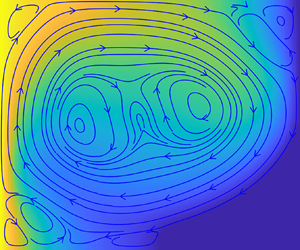
  ${\rm \Delta} T$ between the two vertical walls, reaching a steady state after a sufficiently long time. A series of numerical simulations is conducted, and similar flow patterns are observed. The resultant velocity and temperature fields of one typical case are shown in figure 2(a). This figure reveals that, in addition to the large convective vortex, whose size is comparable to the size of the cavity, four small convective corner rolls also exist due to the confinement of cavity walls, where the flow velocity is low. Moreover, the convective roll at the bottom right corner presents the lowest temperature. Analogically speaking, in the case of melting thermal flow, the solid PCM at the bottom right corner, wherein the thermal convection is also the weakest, will be the most difficult part to be melted.

Figure 2. Steady pure thermal flow at  ${Ra}=2.5 \times 10^4$,
  ${Pr}=0.02$,
  ${Ste}=0.01$ and
  $\gamma =1$. (a) Dimensionless temperature field
  $\theta$ and streamlines. (b) Local temperature profiles at three altitudes. (c) Average thicknesses of TBLs at the left and right walls.
The local temperature profiles at three altitudes,  $y=L_y/4$,
  $L_y/2$ and
  $3L_y/4$, are shown in figure 2(b), and a sandwich structure is observed. Two thermal boundary layers (TBLs) are present at the left and right walls, and their local thicknesses are not equal at the same altitude
  $y$, except at
  $y=L_y/2$. This is due to the local heat accumulation along the flow directions near the vertical walls, as shown in figure 2(a). The local temperature profile in the
  $x$-direction is linear within the TBL, and presents nearly a plateau in between, corresponding to the vortex core. The temperature variation is limited within the two TBLs. Thus the average TBL thickness
  $\delta _T$ can be estimated by extrapolating the temperature profile linearly to
  ${\rm \Delta} T/2$, i.e.
  $\theta = 0.5$:
 \begin{equation} \delta_T ={-}({{\rm \Delta} T}/{2})/({\partial \bar T}/{\partial x}),\end{equation}
where  $\bar T=\int _{0}^{L_y} T \, {\rm d} y /L_y$ is the average temperature over the vertical wall, or the melting interface in the case of melting thermal flows (Belmonte, Tilgner & Libchaber Reference Belmonte, Tilgner and Libchaber1994; Takeshita et al. Reference Takeshita, Segawa, Glazier and Sano1996; Verzicco & Camussi Reference Verzicco and Camussi1999; Zhou et al. Reference Zhou, Stevens, Sugiyama, Grossmann, Lohse and Xia2010; Zhou & Xia Reference Zhou and Xia2010; Scheel & Schumacher Reference Scheel and Schumacher2014; Ng et al. Reference Ng, Ooi, Lohse and Chung2015). Then the total heat transfer rate per unit length injected from the left wall is evaluated as
  $\int _0^{L_y} q_x \,{{\rm d} y} = - \rho C_p \alpha \,( {\partial \bar T}/{\partial x} )\,L_y = \rho C_p \alpha \,{\rm \Delta} T\,{L_y}/({2\delta _T})$, which is indeed independent of the cavity height
  $L_y$ due to the fact that
  $L_y/\delta _T$ is invariant once the Rayleigh number and Prandtl number are given (Shishkina Reference Shishkina2016). Introducing the definition of
  $Nu$ in (2.7a,b), the average Nusselt number is obtained as
 \begin{equation} {Nu} = {L_y}/{(2 \delta_T)}.\end{equation}
As expected, the average thicknesses of the TBLs at the left and right walls are the same (figure 2c), because the energy conservation at the steady state requires that the input energy from the left wall, characterised by  ${Nu}^l=L_y/(2 \delta _{T}^l)$, should be equal to the output energy from the right wall, characterised by
  ${Nu}^r=L_y/(2\delta _{T}^r)$, where
  $\delta _{T}^l$ and
  $\delta _{T}^r$ are the average TBL thicknesses at the left and right walls of the cavity, respectively.
Furthermore, the average Nusselt number can be related to the dimensionless control parameters. For a laminar pure thermal flow, the scaling law for  $Nu$ has been derived theoretically as
  $Nu \sim Ra^{1/4}\,Pr^{1/4}$ for
  $Pr \leq 0.1$, and
  $Nu \sim Ra^{1/4}\,Pr^{0}$ for
  $Pr>0.1$, and validated in the range
  $10^5 \leq Ra \leq 10^{10}$ (Shishkina Reference Shishkina2016). Later, Q. Wang et al. (Reference Wang, Liu, Verzicco, Shishkina and Lohse2021) confirmed this scaling law numerically, providing a scaling law
  $Nu \sim Ra^{0.26}$ for
  $Pr>0.1$. Combining these results, the average Nusselt number is fitted and expressed as
 \begin{equation} Nu =\left\{ \begin{array}{@{}ll} 0.53\,{Ra}^{1/4}\,{Pr}^{1/4}, & {\rm if} \ {Pr}\leq0.1,\\[2pt] 0.24\,{Ra}^{0.26}\,{Pr}^0, & {\rm elsewhere.} \end{array}\right.\end{equation}
It is worth noticing that the theoretically predicted scaling  $Nu \sim Ra^{1/4}$ at
  $Pr>0.1$ also fits the data reported by Shishkina (Reference Shishkina2016) and Q. Wang et al. (Reference Wang, Liu, Verzicco, Shishkina and Lohse2021), and presents a negligible difference from
  $Nu \sim Ra^{0.26}$ at high
  $Ra$. However, at low
  $Ra$,
$Ra$,  $Nu \sim Ra^{1/4}$ shows a noticeable deviation with respect to the previous data, as observed by Q. Wang et al. (Reference Wang, Liu, Verzicco, Shishkina and Lohse2021). Thus we choose to employ
  $Nu \sim Ra^{0.26}$ at
  $Pr>0.1$, as in (2.10).
According to (2.9), the average TBL thickness normalised by  $L_y$ is then
 \begin{equation} \frac{\delta_T}{L_y} =\left\{ \begin{array}{@{}ll} 0.94\,{Ra}^{{-}1/4}\,{Pr}^{{-}1/4}, & {\rm if} \ {Pr}\leq0.1,\\[2pt] 2.08\,{Ra}^{{-}0.26}\,{Pr}^0, & {\rm elsewhere,} \end{array}\right.\end{equation}
predicting  $\delta _T/L_y=0.1988$ for
  ${Ra}=2.5 \times 10^4\ {\rm and} {Pr}=0.02$, which is in good agreement with the numerical result (figure 2c).
For the melting thermal flow, simulations are conducted under the same boundary conditions as those for the pure thermal flow, except that the cavity is initially filled with solid PCM, and an evolving melting interface exists. In the simulations, the melting interface is located by connecting the mesh points with a local melting fraction  $1/2$, and will overlap with the right cold wall at the end of the melting process.
The interface evolution behaviours and corresponding thermal flow dynamics are similar in different simulations.To illustrate the melting process, the time evolution of the melting interface for a typical case, with the accompanying flow and temperature fields appended, is shown in figures 3(a–c). These melting processes are usually interpreted by the well-known two-stage melting model (Bareiss & Beer Reference Bareiss and Beer1984; Ho & Viskanta Reference Ho and Viskanta1984; Gau & Viskanta Reference Gau and Viskanta1986; Wolff & Viskanta Reference Wolff and Viskanta1988; Bertrand et al. Reference Bertrand1999; Wang et al. Reference Wang, Amiri and Vafai1999; Du et al. Reference Du, Yuan, Jia, Cheng and Mao2007; Huang et al. Reference Huang, Wu and Cheng2013; Shokouhmand & Kamkari Reference Shokouhmand and Kamkari2013; Li et al. Reference Li, Yang and Zhang2014; Luo et al. Reference Luo, Yao, Yi and Tan2015; Hamad et al. Reference Hamad, Egelle, Cummings and Russell2017, Reference Hamad, Egelle, Gooneratne and Russell2021). In the first stage, the melted liquid layer is thin; thus the viscosity dominates the flow. Accordingly, the heat is transferred via conduction; therefore the melting interface remains parallel with the left wall (figure 3a). As time goes by, the melted liquid layer thickens increasingly, and the buoyancy gradually overcomes the viscosity to dominate the flow. Consequently, the rising hot liquid continuously scours the upper region of the PCM, and generates a distorted melting interface (figure 3b). In this second stage, thermal convection comes into play and eventually dominates the heat transfer. In addition, a part of the right cold wall will be exposed directly to the hot melted liquid during the final phase of the melting process (figure 3c), as observed in the existing studies (Bénard et al. Reference Bénard, Gobin and Martinez1985; Duan et al. Reference Duan, Xiong and Yang2019; Rakotondrandisa et al. Reference Rakotondrandisa, Danaila and Danaila2019; Yang et al. Reference Yang, Guo, Liu, Jin and He2019). In these studies, this final phase of the melting process is considered to be the last part of the second convection stage. However, their  $f_l$ versus
  $Fo_x$ curves reveal that the melting rate
  $\partial f_l/ \partial {Fo_x}= \partial (s/L_x)/ \partial {Fo_x}$ will decrease significantly as in figure 3(e) once the cold cavity wall is exposed to the melted liquid, indicating the change in heat transfer characteristics. Thus introducing a third stage is necessary to characterise the melting process. Meanwhile, in the bottom right corner where the remnant solid PCM is left, the thermal convection will decay significantly as informed by the discussions on the pure thermal flow. Thus this third stage is referred to as ‘the decaying convection stage’. Consequently, the traditional two-stage model should be updated to a three-stage melting model, including conduction, convection and decaying convection.

Figure 3. Melting thermal flow at  $Ra = 2.5 \times 10^4$,
  $Pr = 0.02$,
  $Ste = 0.01$ and
  $\gamma = 1$. (a–c) Dimensionless temperature fields and streamlines. (d) Horizontal intersection between solid PCM and the bottom wall (
 $x_0$) from present simulation (circles), from Rakotondrandisa et al. (Reference Rakotondrandisa, Danaila and Danaila2019) (squares), and from Bénard et al. (Reference Bénard, Gobin and Martinez1985) (triangles). (e) Comparison between average thicknesses of TBLs (
 $\delta _{T}^l$ and
  $\delta _{T}^i$) and the average thickness of the melted liquid layer (
 $s$). Three melting stages are in turn labelled in orange, green and grey in the background. (f) The average Nusselt number
  $Nu$ obtained from the melting thermal flows performed by Webb & Viskanta (Reference Webb and Viskanta1986) (circles) and Rakotondrandisa et al. (Reference Rakotondrandisa, Danaila and Danaila2019) (triangles). The red dashed line is
  $Nu$ scaling (see (2.10)) developed in the pure thermal flow by Shishkina (Reference Shishkina2016).
For the thermal convection, it is found that the convection intensity gathers mainly at the upper part of the cavity due to the buoyancy in the second and third stages, and becomes negligible close to the bottom wall (figures 3b,c). That is, the propagation of the horizontal intersection  $x_0$ between solid PCM and the cavity bottom wall is driven by conduction, indicating
  $x_0/L_x \sim \sqrt {Fo_x}$ as stated by Hamdan & Elwerr (Reference Hamdan and Elwerr1996) and Hamdan & Al-Hinti (Reference Hamdan and Al-Hinti2004). To have a convincing validation,
  $x_0$ from the presented simulation in figures 3(a–c) and those reported in the studies of Rakotondrandisa et al. (Reference Rakotondrandisa, Danaila and Danaila2019) and Bénard et al. (Reference Bénard, Gobin and Martinez1985), are normalised by
  $L_x$ and presented as functions of
  $Fo_x$ as shown in figure 3(d). Accordingly, the fitting correlations of the three data sets are
  $x_0/L_x=0.13\,Fo_x^{0.50}$,
  $x_0/L_x=0.25\,Fo_x^{0.52}$ and
  $x_0/L_x=0.52\,Fo_x^{0.53}$, where the scaling exponents are very close to the expected value of
  $1/2$, and increase very slightly when
  $Ra$ varies widely from
  $10^4$ to
  $10^9$. This finding indicates that the conduction dominance at the bottom wall is reasonable.
The following discusses the TBLs in the melting thermal flow. In figure 3(e), the average thickness of the TBL at the left wall ( $\delta _{T}^l$) and that at the melting interface (
 $\delta _{T}^i$) are shown for the melting case presented in figures 3(a–c). Meanwhile, the average thicknesses of the melted liquid layer (
 $s$) from the present simulation and those from Huang et al. (Reference Huang, Wu and Cheng2013) are also appended for comparison, wherein a good agreement is achieved. For the configuration under consideration, the first stage lasts for
  ${Fo_x} \leq 2.7$ (figure 3e), where the melted liquid layer is saturated with TBLs, i.e.
  $s=\delta _{T}^l+\delta _{T}^i$, verifying the dominance of conduction in the heat transfer mechanism. In the second stage (
 $2.7< Fo_x \leq 25.9$), thermal convection is sufficiently strong to separate the two TBLs; thus
  $s>\delta _{T}^l+\delta _{T}^i$, constituting a sandwich structure as well. In the third stage (
 $Fo_x>25.9$),
  $s>\delta _{T}^l+\delta _{T}^i$ still holds, while
  $\delta _{T}^i$ in this stage comprises two parts: TBLs along the liquid–solid PCM interface and the uncovered right cold wall (figure 3c). As for the relation between
  $\delta _{T}^l$ and
  $\delta _{T}^i$, it is found that they are approximately equal to each other, rather than the identical equality as observed in the pure thermal flow (figure 2c). Such an approximately equal behaviour can also be explained from the viewpoint of energy conservation. PCM melting is an unsteady process, wherein the bulk temperature of the melted liquid varies over time. Consequently, the input energy, characterised by
  ${Nu}^l=L_y/(2 \delta _{T}^l)$, is divided into two parts: one is responsible for the variation of the bulk temperature of the melted liquid, corresponding to the sensible heat; the other is transferred to the melting interface, characterised by
  ${Nu}^i=L_y/(2\delta _{T}^i)$, to compensate for the melting latent heat or the leaking energy through the uncovered right cold wall. The sensible heat is negligible due to the low Stefan number under consideration, resulting in
  ${Nu}^l \approx {{Nu}}^i$; thus
  $\delta _{T}^l \approx \delta _{T}^i$. The approximately equal
  $Nu^l \approx Nu^i$ has also been reported by Bénard et al. (Reference Bénard, Gobin and Martinez1985), wherein
  $Ste = 0.084$.
Furthermore, it is easy to conclude that the average thickness of the TBL is  $\delta _{T}^l=\delta _{T}^i=s/2$ in the conduction-dominated first stage, after which a comparison between figures 2(c) and 3(e) shows that the average TBL thicknesses in the melting thermal flow are approximate to those in the corresponding pure thermal flow. In addition to the data in the present study, the results from the existing studies are also presented in figure 3(f). The averaged Nusselt number in the melting thermal flows reported by Webb & Viskanta (Reference Webb and Viskanta1986) and Rakotondrandisa et al. (Reference Rakotondrandisa, Danaila and Danaila2019) are approximately equal to their counterparts in pure thermal flows, as discussed by Shishkina (Reference Shishkina2016). Considering
  $Nu=L_y/(2\delta _T)$, the averaged TBL thicknesses in a melting thermal flow are approximately equal to those in the pure thermal flow under the same configurations. Herein, the approximate equality is attributed to the energetically expensive PCM melting at low
  ${Ste}$; thus a time scale separation between the thermal convection and the melting interface migration exists. That is, thermal convection at low
  $Ste$ would adapt rapidly to the melting interface migration, being in a nearly quasi-steady state. Thus approximately equal average TBL thicknesses are observed in melting and pure thermal flows under the same configurations. This approximate equality has also been observed in pure and melting Rayleigh–Bénard convections (Esfahani et al. Reference Esfahani, Hirata, Berti and Calzavarini2018).
In summary, a comparison with the pure thermal flow deepens the understanding of the melting thermal flow, and the following conclusive points, which will inform the theoretical modelling in the subsequent section, are realised. (I) In addition to the conduction–convection two-stage description, a third melting stage is suggested, wherein the melting rate decreases continuously until the end of the melting process. (II) The propagation of the horizontal intersection  $x_0$ between solid PCM and the cavity bottom wall is driven by heat conduction. (III) The average thickness of the TBL at the left wall (
 $\delta _{T}^l$) and that at the melting interface (
 $\delta _{T}^i$) are approximately equal at low
  $Ste$. (IV) In the first stage, the average thickness of the TBL is
  $\delta _T=s/2$, and after this stage, the averaged TBL thickness in the melting thermal flow is approximately equal to that in the pure thermal flow under the same configurations.
3. Predictions
Theoretical analyses on the melting problem presented in § 2.1 are performed in this section, based on the discussions in § 2.2.
The vicinity region within the TBL is examined to describe the evolution of the melting interface. The vertically averaged position of the melting interface (dashed line in figure 1) is denoted by  $s$. The velocity
  $\boldsymbol {u}$ is negligible when the melted liquid flow is close to the interface, due to the no-slip condition therein. Accordingly, (2.3) in the limit of
  $x\to s$ simplifies to
 \begin{equation} \frac{\partial T}{\partial t} + \frac{\mathcal{L} }{C_p}\, \frac{\partial f_l }{\partial t} = \alpha\,{\nabla}^2 T .\end{equation}
 In addition to  $\theta$, the following dimensionless quantities are further introduced:
 \begin{equation} x'=x/\delta_T, \quad y'=y/L_y \quad {\rm and} \quad t'=t/t_0, \end{equation}
where  $t_0$ is the characteristic time necessary to achieve a melted liquid fraction of
  $f_l$. Equation (3.1) is then normalised as follows:
 \begin{equation} \frac{\partial \theta}{\partial t'} + \frac{1}{ {Ste} }\, \frac{\partial f_l}{\partial t'} =\frac{\alpha t_0}{\delta_T^2} \left( \frac{\partial^2 \theta}{\partial x'^2} +\frac{\delta_T^2}{L_y^2}\,\frac{\partial^2 \theta}{\partial y'^2}\right).\end{equation}
On the one hand, thermal energy for a PCM is stored mainly in the form of latent heat rather than sensible heat. It thus leads to  $1/ {Ste} \gg 1$, indicating that the first unsteady term on the left-hand side is negligible compared with the second one. On the other hand, the average thickness
  $\delta _T$ of the TBL is usually substantially smaller than the cavity length scale
  $L_y$. Thus only the temperature gradient along the
  $x$-direction is retained in the diffusive term. Therefore, (3.3) is further simplified to
 \begin{equation} \frac{1}{ {Ste} }\,\frac{\partial f_l}{\partial t'} = \frac{\alpha t_0}{\delta_T^2}\,\frac{\partial^2 \theta}{\partial x'^2},\end{equation}
and its dimensional form is
 \begin{equation} \mathcal{L}\,\frac{\partial f_l}{\partial t} =C_p \alpha\, \frac{\partial^2 T}{\partial x^2}.\end{equation}
That is, the latent heat necessary for the PCM melting is compensated by the thermal diffusion in the  $x$-direction. Integrating the above equation over the cavity (
 $0 \leq x \leq L_x$,
  $0 \leq y \leq L_y$) as in the previous studies (Esfahani et al. Reference Esfahani, Hirata, Berti and Calzavarini2018; Favier et al. Reference Favier, Purseed and Duchemin2019), the following can be obtained:
 \begin{equation} \mathcal{L}\,\frac{\partial f_l}{\partial t}\,L_x L_y =C_p \alpha \int_{0}^{L_y} \left[ \left(\frac{\partial T}{\partial x}\right)_r- \left(\frac{\partial T}{\partial x}\right)_l \right] \rm{d}y,\end{equation}
where the subscripts ‘ $r$’ and ‘
 $l$’ denote the right (
 $x=L_x$) and left (
 $x=0$) walls, respectively,
  $-C_p \alpha \int _{0}^{L_y} ({\partial T}/{\partial x})_l \,\rm {d} y >0$ is the input energy, and
  $C_p \alpha \int _{0}^{L_y} ({\partial T}/{\partial x})_r \, \rm {d} y \leq 0$ is the leaking energy through the right cold wall.
3.1. Predictions for the first and second stages
Three stages are identified for the PCM melting in a rectangle cavity. This subsection considers the first and second stages, where the right wall of the cavity is covered entirely by the solid PCM with the same temperature  $T_m$; thus no energy leaks out. This leads from (3.6) to
 \begin{equation} \mathcal{L}\,\frac{\partial f_l}{\partial t}\,L_x L_y ={-}C_p \alpha \left(\frac{\partial \bar T}{\partial x}\right)_l L_y.\end{equation}
Considering  $f_l=s/L_x$, this equation becomes
 \begin{equation} \frac{\partial s }{\partial t} ={-}\frac{C_p \alpha }{\mathcal{L}} \left(\frac{\partial \bar T}{\partial x}\right)_l= \frac{C_p \alpha }{\mathcal{L}}\,\frac{ {\rm \Delta} T}{2 \delta_T},\end{equation}
where (2.8) is used to relate  $\delta _T$ and the average temperature gradient. It should be noted that (3.8) is applicable for only the first and second stages. In the third stage, a part of the right cold wall is directly exposed to the melted liquid (figure 3c), thus inducing energy leakage. Then (3.6) becomes
  $\mathcal {L}\,({\partial f_l}/{\partial t})\,L_x L_y < -C_p \alpha \,({\partial \bar T}/{\partial x})_l\,L_y$, explaining the melting rate in the third stage being smaller than that (see (3.7)) in the second stage, as observed in figure 3(e) and existing studies (Bénard et al. Reference Bénard, Gobin and Martinez1985; Duan et al. Reference Duan, Xiong and Yang2019; Rakotondrandisa et al. Reference Rakotondrandisa, Danaila and Danaila2019; Yang et al. Reference Yang, Guo, Liu, Jin and He2019).
Section 2.2 concluded that after the first stage, the average thickness of the TBL in a melting thermal flow is approximately equal to that (see (2.11)) in the pure thermal flow under the same configuration. Meanwhile,  $\delta _T = s/2$ in the first stage; thus the average TBL thickness in melting thermal flows can be summarised as
 \begin{equation} \delta_T = \min (s/2, kL_y\,{Ra}^m\,{Pr}^n),\end{equation}
where  $k=0.94$,
  $m=-0.25$,
  $n=-0.25$ for
  ${Pr}\leq 0.1$, and
  $k=2.08$,
  $m=-0.26$,
  $n=0$ for
  ${Pr}>0.1$, as indicated in (2.11).
Substituting (3.9) into (3.8), the average thickness of the melted liquid layer  $s$ is then obtained by integration as
 \begin{equation} s =\left\{ \begin{array}{@{}ll} \sqrt{2 \alpha t\,{Ste} }, & {\rm if} \ s \leq 2 k L_y\,{Ra}^{m}\,{Pr}^n,\\[3pt] \dfrac{\alpha t\,{Ste} }{2 k L_y\,{Ra}^m\,{Pr}^n} + k L_y\,{{Ra}^{m}\,{Pr}^n}, & {\rm elsewhere,} \end{array}\right.\end{equation}
where we have imposed the boundary conditions that  $s (t=0)=0$ and
  $s$ is a continuous function with respect to
  $t$. Consequently, the melted liquid fraction
  $f_l$ during the first and second stages is derived macroscopically as
 \begin{equation} f_l =\frac{s}{L_x}=\left\{ \begin{array}{@{}ll} \sqrt{2\,{Fo_x}\,{Ste}}, & {\rm if} \ f_l \leq 2 k\,{Ra}^{m}\,{Pr}^n / \gamma,\\[2pt] \gamma\,{Fo_x}\,{Ste} / (2 k\,{Ra}^m\,{Pr}^n) + k\,{Ra}^m\,{Pr}^n / \gamma, & {\rm elsewhere}, \end{array}\right.\end{equation}
where  $s /L_y =\gamma s/L_x =\gamma f_l$ were used.
3.2. Prediction for the third stage
In the third stage, the upper part of the cavity right cold wall is exposed to the hot liquid PCM, and the remnant solid PCM is located in the bottom right corner, which is simplified into a rectangle with  $x_0 \leq x \leq L_x$ and
  $0 \leq y \leq y_0$, as shown in figure 4(a). In this stage, the energy reaching the melting interface is divided into two parts (figure 4a): the part at
  $0 \leq y \leq y_0$ drives the PCM melting, and the other part at
  $y_0 \leq y \leq L_y$ leaks out through the uncovered right cold wall. Thus the leaking energy can be estimated as
  $C_p \alpha \,({\partial \bar T}/{\partial x})_i\,(L_y-y_0)$, with the subscript ‘
 $i$’ denoting the melting interface. Substituting this estimation into (3.6), one gets
 \begin{equation} \mathcal{L}\,\frac{\partial f_l}{\partial t}\,L_x L_y = C_p \alpha \left(\frac{\partial \bar T}{\partial x}\right)_i (L_y-y_0)-C_p \alpha\left(\frac{\partial \bar T}{\partial x}\right)_l L_y ={-}C_p \alpha \left(\frac{\partial \bar T}{\partial x} \right)_l y_0,\end{equation}
where the equation on the right is obtained from that at low  $Ste$,
  $\delta _T^l \approx \delta _T^i$; thus
  $({\partial \bar T}/{\partial x})_l \approx ({\partial \bar T}/{\partial x})_i$, as discussed in § 2.2.

Figure 4. (a) Schematic of the PCM melting during the third stage, where the red line is the melting interface, and its upper part ( $y_0 \leq y \leq L_y$) overlaps the uncovered right cold wall. (b) Melting rate of three stages normalised by that of the second stage. In addition to the present simulations (circles and squares), the results from Bénard et al. (Reference Bénard, Gobin and Martinez1985) (triangles) and Huang et al. (Reference Huang, Wu and Cheng2013) (stars) are also presented.
Equations (3.7) and (3.12) indicate that the melting rate ( $\partial f_l /\partial t$) depends only on the averaged input heat flux
  $-C_p \alpha \,({\partial \bar T}/{\partial x})_l=C_p \alpha \,{{\rm \Delta} T}/({2 \delta _T})$, and the vertical projected areas of the solid PCM, which are
  $L_y$ and
  $y_0$ in the first two stages and the third one, respectively. This is consistent with the result of Baehr & Stephan (Reference Baehr and Stephan2011), who showed that the thermal power, proportional to the melting rate in the present study, is determined by the dot product between the average input heat flux (
 $\boldsymbol {q}$) and the surface element (
 $\boldsymbol {A}$) as
  $\boldsymbol {q} \boldsymbol {\cdot } \boldsymbol {A}=|\boldsymbol {q}|\,|\boldsymbol {A}| \cos \psi$, thus depending on the projected area
  $|\boldsymbol {A}| \cos \psi$ rather than the absolute area
  $|\boldsymbol {A}|$. Here,
  $\psi$ is the local intersection angle between
  $\boldsymbol {q}$ and
  $\boldsymbol {A}$.
In addition,  $\delta _T$ in the second and third stages is approximately the same (figures 3e,f), because in these two stages the thermal convection takes effect and the characteristic convection velocity (
 $\sqrt {|\boldsymbol {g}|\beta \,{\rm \Delta} T\,L_y}$) is invariant, resulting in an unchanged average TBL thickness
  $\delta _T$. Thus (3.12) can be divided by (3.7) to cancel out the average temperature gradient, resulting in
 \begin{equation} \left.\left(\frac{\partial f_l}{\partial t}\right)_3 \right/ \left(\frac{\partial f_l}{\partial t}\right)_2 =\frac{y_0}{L_y}, \end{equation}
where subscripts ‘2’ and ‘3’ denote the second and third stages, respectively. This equation indicates clearly that the melting rate in the third stage will gradually decrease compared with that in the second one, because  $y_0$ will gradually move downwards as the melting continues. Therefore, this equation attributes the continuously decreasing melting rate in the third stage to the decrease in the vertical projected area, which, relatively speaking, is more direct in understanding than the explanation by Shokouhmand & Kamkari (Reference Shokouhmand and Kamkari2013). They explained that the decreasing melting rate is attributed to the depression of the convection current, due to the increase in the bulk temperature of liquid PCM and the stratification of temperature fields.
Close to the bottom wall, heat transfer is dominated by conduction (Hamdan & Elwerr Reference Hamdan and Elwerr1996), as discussed in § 2.2. Introducing the values of  ${Ste}$ in figure 3(d) into the first branch of (3.10), the horizontal intersections are calculated as
  $x_0/L_x=s/L_x=0.14\sqrt {Fo_x}$,
  $x_0/L_x=s/L_x=0.30 \sqrt {Fo_x}$ and
  $x_0/L_x=s/L_x=0.41\sqrt {Fo_x}$, where the multiplicative factors (0.14, 0.30 and 0.41) are respectively close to the fitting coefficients 0.13, 0.25 and 0.52 in figure 3(d). Thus the horizontal intersection
  $x_0 = s$ can be calculated from the present conduction solution, yielding
 \begin{equation} x_0 = L_x\sqrt{2 {Fo_x} \, {Ste}}. \end{equation}
The vertical intersection  $y_0$ between solid PCM and the right wall (figure 4a) is estimated from the definition of melted liquid fraction
  $f_l = 1-{(L_x-x_0)y_0}/{(L_x L_y)}$ as
 \begin{equation} \frac{y_0}{L_y} = \frac{1-f_l}{1-\sqrt{2 {Fo_x} \, {Ste} }}.\end{equation}
During the second stage, the melting rate  ${\partial f_l}/{\partial {Fo_x}}$ is obtained from the second branch of (3.11) as
 \begin{equation} \left( \frac{\partial f_l}{\partial {Fo_x}} \right)_2 = \frac{\gamma\,{Ste}}{2 k\,{Ra}^m\,{Pr}^n},\end{equation}
which is obviously a constant over time. Then, according to (3.13), the melting rate in the third stage is evaluated as
 \begin{equation} \left( \frac{\partial f_l}{\partial {Fo_x}} \right)_3= \frac{y_0}{L_y}\,\frac{\gamma\,{Ste}}{2 k\,{Ra}^m\,{Pr}^n}= \frac{1-f_l}{1-\sqrt{2 {Fo_x} \, {Ste} }}\, \frac{\gamma\,{Ste}}{2 k\,{Ra}^m\,{Pr}^n},\end{equation}
where (3.15) and (3.16) were introduced. Assuming that the third stage starts from the point  $(Fo_{x}^c,\,f_{l}^c )$, an integration of (3.17) then gives
 \begin{align} f_l = 1- (1-f_{l}^c) \left(\frac{1-\sqrt{2 {Fo_x} \, {Ste} }}{1- \sqrt{2 {Fo_{x}^c} \, {Ste} }} \right)^{{\gamma}/{(2 k\,{Ra}^m\,{Pr}^n)}} \exp \left[\frac{\gamma (\sqrt{2 {Fo_x} \, {Ste} } - \sqrt{2 {Fo_{x}^c} \, {Ste} })}{2 k\,{Ra}^m\,{Pr}^n} \right]. \end{align}
In order to predict  $f_l^c$, the melting rate of the entire melting process is divided by that of the second stage as
  $({\partial f_l}/{\partial Fo_x}) / ({\partial f_l}/{\partial Fo_x} )_2$, as shown in figure 4(b). In this figure, a very short transition from the second to the third stages is observed, where the ratio sharply decreases from 1 to around 0.5. As denoted by (3.13), this ratio after the second stage is equal to
  $y_0/L_y$. Therefore, the sharp decrease indicates that the vertical intersection between solid PCM and the right wall moves downwards rapidly when
  $y_0/L_y>0.5$. This is quite reasonable because the thermal convection intensity concentrates mainly on the upper part of the cavity due to buoyancy. Meanwhile, the transition is very short-lived; therefore it is reasonable to assume that the starting point of the third stage is also the end point of the second stage. Thus the transition point
  $(Fo_x^c,f_l^c)$ satisfies the equations
 $$\begin{gather} \left(\frac{y_0}{L_y}\right)_c = \frac{1-f_l^c}{1-\sqrt{2 {Fo_x^c} \, {Ste} }} \approx \frac{1}{2}, \end{gather}$$
 $$\begin{gather}f_l^c = \gamma\,{Fo_x^c}\,{Ste} / (2 k\,{Ra}^m\,{Pr}^n) + k\,{Ra}^m\,{Pr}^n / \gamma, \end{gather}$$
where the second equation is the second branch of (3.11). Combining the two equations above, the following is obtained:
 \begin{equation} \left. \begin{array}{l} f_l^c = \tfrac{1}{2}+\sqrt{\mathcal{A}+\mathcal{B}}, \\ \mathcal{A} =\tfrac{1}{2} k\,Ra^m\,Pr^n\,(\gamma-k\,Ra^m\,Pr^n)/ \gamma^2, \\ \mathcal{B}=\tfrac{1}{2} k \sqrt{2 \gamma k\,Ra^{3m}\,Pr^{3n}-3k^2\,Ra^{4m}\, Pr^{4n}}/\gamma^2\end{array} \right\}\end{equation}
and
 \begin{equation} {Fo}_x^c=2k\,{Ra}^m\,{Pr}^n\,(\,f_{l}^c-k\,{Ra}^m\,{Pr}^n/\gamma)/(\gamma\,{Ste}). \end{equation}
The onset of the third stage,  $(\,f_{l}^c, Fo_{x}^c)$, has now been determined. Further combining (3.11) and (3.18), the full prediction for the melted liquid fraction at all stages is obtained as
 \begin{align} f_l =\left\{
\begin{array}{@{}ll} \sqrt{2 {Fo_x} \, {Ste} }, & {\rm if}\ f_l
\leq 2
k\,{Ra}^{m}\,{Pr}^n /
\gamma,\\
\gamma\,{Fo_x}\,{Ste} / (2
k\,{Ra}^m\,{Pr}^n) +
k\,{Ra}^m\,{Pr}^n /
\gamma, & {\rm if} \ 2
k\,{Ra}^{m}\,{Pr}^n /
\gamma \leq f_l \leq f_{l}^{c},\\
\begin{aligned} & 1- (1-f_{l}^c) \left(\dfrac{1-\sqrt{2
{Fo_x} \, {Ste} }}{1- \sqrt{2 {Fo_{x}^c} \, {Ste} }}
\right)^{{\gamma}/{(2
k\,{Ra}^m\,{Pr}^n)}}\\ & \quad
\times \exp\left[\dfrac{\gamma (\sqrt{2 {Fo_x} \,
{Ste} } - \sqrt{2 {Fo_{x}^c} \, {Ste} })}{2
k\,{Ra}^m\,{Pr}^n}\right],\end{aligned} & {\rm elsewhere}.
\end{array}\right.
\end{align}
\begin{align} f_l =\left\{
\begin{array}{@{}ll} \sqrt{2 {Fo_x} \, {Ste} }, & {\rm if}\ f_l
\leq 2
k\,{Ra}^{m}\,{Pr}^n /
\gamma,\\
\gamma\,{Fo_x}\,{Ste} / (2
k\,{Ra}^m\,{Pr}^n) +
k\,{Ra}^m\,{Pr}^n /
\gamma, & {\rm if} \ 2
k\,{Ra}^{m}\,{Pr}^n /
\gamma \leq f_l \leq f_{l}^{c},\\
\begin{aligned} & 1- (1-f_{l}^c) \left(\dfrac{1-\sqrt{2
{Fo_x} \, {Ste} }}{1- \sqrt{2 {Fo_{x}^c} \, {Ste} }}
\right)^{{\gamma}/{(2
k\,{Ra}^m\,{Pr}^n)}}\\ & \quad
\times \exp\left[\dfrac{\gamma (\sqrt{2 {Fo_x} \,
{Ste} } - \sqrt{2 {Fo_{x}^c} \, {Ste} })}{2
k\,{Ra}^m\,{Pr}^n}\right],\end{aligned} & {\rm elsewhere}.
\end{array}\right.
\end{align}
This prediction contains the effects of all dimensionless control numbers under consideration, and is valid when  ${Ste}$ is sufficiently small. The upper limit of
  $Ste$ will be discussed in the next subsection.
3.3. Validation
In this subsection, the predicted melted liquid fraction  $f_l$ (see (3.23)) is validated by comparing with the reported data, which are mainly from the previous studies listed in table 1. Note that the numerical data obtained by Jany & Bejan (Reference Jany and Bejan1988) cited in table 1 are not employed herein, because their correlation (and thus the numerical data) greatly overestimates the existing experiment and numerical results, as indicated by Duan et al. (Reference Duan, Xiong and Yang2019). Moreover, the experimental studies by Wolff & Viskanta (Reference Wolff and Viskanta1988), Wang et al. (Reference Wang, Amiri and Vafai1999) and Du et al. (Reference Du, Yuan, Jia, Cheng and Mao2007) used multiple group data to fit their
  $f_l$ correlations. However, the authors did not provide complete information regarding dimensionless control parameters; thus their data are not employed herein either. In order to perform a thorough validation, the numerical results from Huang et al. (Reference Huang, Wu and Cheng2013) and Rakotondrandisa et al. (Reference Rakotondrandisa, Danaila and Danaila2019) are also supplemented.
The collected reported data cover a wide range of dimensionless control parameters (Ho & Viskanta Reference Ho and Viskanta1984; Bénard et al. Reference Bénard, Gobin and Martinez1985; Gau & Viskanta Reference Gau and Viskanta1986; Brent et al. Reference Brent, Voller and Reid1988; Chakraborty & Chatterjee Reference Chakraborty and Chatterjee2007; Huang et al. Reference Huang, Wu and Cheng2013; Duan et al. Reference Duan, Xiong and Yang2019; Faden et al. Reference Faden, Linhardt, Höhlein, König-Haagen and Brüggemann2019; Rakotondrandisa et al. Reference Rakotondrandisa, Danaila and Danaila2019), namely  $2.5\times 10^5 \leq {Ra} \leq 1.09 \times 10^9$,
  $0.02 \leq {Pr} \leq 56.2$,
  $0.01 \leq {Ste} \leq 0.132$ and
  $0.3876 \leq \gamma \leq 1.4$. Figure 5 shows that although the reported data resulted in a series of different fitting correlations as summarised in table 1, all these data can be predicted by the present solution (see (3.23)). By contrast, the prediction accuracy in the third stage is less satisfying than that in the first and second stages (figures 5d–f). This is probably due to the rectangular simplification of remnant solid PCM (figure 4a), and the approximation in the derivation of
  $\,f_{l}^{c}$ (see (3.19)). Nevertheless, in the present validation, the maximum relative error
  $E_r=\{|f_l^p-f_l^t|/f_l^t\}_{max}$ in the third stage is still within
  $10\,\%$, where the superscripts‘
 $p$’ and ‘
 $t$’ represent the prediction and reported results, respectively.

Figure 5. The predictions are tested against the reported data available with different PCMs: (a) and (b) n-octadecane; (c) gallium; (d) tin; (e) and (f) n-octadecane. In all panels, the orange, green and grey backgrounds are used to denote the first (conduction), the second (convection) and the third (decaying convection) stages, respectively.
The previous section indicated that the prediction (3.23) is valid only at low Stefan numbers. We discuss now its upper limit in a numerical way due to the lack of reported experimental measurements. In figure 6, the predicted  $f_l$ is compared to the simulated data. As expected, the relative error between the present solution and the simulation result rises as
  ${Ste}$ increases. It is found that
  ${Ste}$ should not exceed
  $0.3$, when the maximum relative error
  $E_r$ is required to be less than 10
  $\%$.
$\%$.

Figure 6. The upper limit of  $Ste$. Simulations and predictions are performed with
  ${Ra}=1.0 \times 10^5$,
  ${Pr}=0.02$ and
  $\gamma =1.0$: (a)
  ${Ste}=0.2$, (b)
  ${Ste}=0.3$, and (c)
  ${Ste}=0.4$.
4. Discussions
This section will first explain further the effect of the distorted melting interface. Parameter space and 3-D effect will then be discussed, and transitions between the two successive stages will be discussed as well in the end.
4.1. Effect of the distorted melting interface
During the melting process, the geometry of the melted liquid layer, characterised by the melting interface, is evolving continuously, and its influence on melted liquid flow and heat transfer is incorporated in the derivation implicitly, by the average input heat flux ( $C_p \alpha {{\rm \Delta} T}/{(2 \delta _T)}$) and the vertical projected area of the solid PCM. The two factors determine the melting rate uniquely, as mentioned previously.
In the first and second stages, the solid PCM occupies the entire right cold wall, and the vertical projected area is always  $L_y$, regardless of whether the melting interface is distorted or not. Thus the influence of altered geometry is exerted on the melting rate by changing the average input heat flux, which is incorporated in the model via the average thickness of the TBL,
  $\delta _T = \min (s/2, kL_y\,{Ra}^m\,{Pr}^n)$ (see (3.9)). This expression indicates that in the first stage, the heat conduction will increase the aspect ratio of the melted liquid geometry (
 $s/L_y$), and thus thicken the TBL. In the second stage, the altered geometry will not change the average thickness of the TBL, because during this stage, thermal convection takes effect and the characteristic convection velocity (
 $\sqrt {|\boldsymbol {g}|\beta \,{\rm \Delta} T\,L_y}$) is irrelevant to
  $s$, resulting in the fact that
  $\delta _T$ is also independent of
  $s$. In the third stage, the average input heat flux also remains unchanged, for the same reason as in the second stage. Thus the influence of altered geometry is realised by changing the vertical projected area, which is
  $y_0$ in this stage and has been incorporated in the prediction for
  $f_l$ via the melting rate ratio (3.17).
In the derivation, the melting interface position is simplified as the average thickness of the melted liquid layer ( $s$). This simplification removes the effect of interface curvature in the second and third stages, but its influence on the
  $f_l$ solution is negligible. This is because the interface distortion does not change the vertical projected area of solid PCM and influences only rather trivially the average input heat flux in the melting thermal flow, compared with that in the pure thermal flow, as shown in figure 3(f).
4.2. Parameter space and 3-D effect
In this study, (3.8) is the central equation in the modelling, relating the average thickness of the melted liquid layer to the average thickness of the TBL, which is obtained by normalising the energy equation (2.3) at a low Stefan number (the upper limit  $Ste \leq 0.3$ is deduced with an allowable error of
  $E_r<$10 % a posteriori). Then the solutions of
  $f_l$ in the first and second stages are solved directly from (3.8), with the average TBL thickness (
 $\delta _T$) determined from the scaling law of
  $Nu$ in a laminar flow regime, which is derived and validated in the range
  $10^5 \leq Ra \leq 10^{10}$ by Shishkina (Reference Shishkina2016). In the third stage,
  $f_l$ cannot be solved by (3.8) due to the leaking energy, which instead is modelled by establishing the relation of melting rate between the second and third stages (see (3.17)), where no extra restrictive condition is introduced. Thus the parameter space to which the predictions in this study are applicable corresponds to a laminar melting process with
  $Ra \leq 10^{10}$ and
  $Ste \leq 0.3$. This parameter space is consistent with the existing studies (Ho & Viskanta Reference Ho and Viskanta1984; Bénard et al. Reference Bénard, Gobin and Martinez1985; Gau & Viskanta Reference Gau and Viskanta1986; Webb & Viskanta Reference Webb and Viskanta1986; Brent et al. Reference Brent, Voller and Reid1988; Jany & Bejan Reference Jany and Bejan1988; Wolff & Viskanta Reference Wolff and Viskanta1988; Wang et al. Reference Wang, Amiri and Vafai1999; Chakraborty & Chatterjee Reference Chakraborty and Chatterjee2007; Huang et al. Reference Huang, Wu and Cheng2013; Luo et al. Reference Luo, Yao, Yi and Tan2015; Duan et al. Reference Duan, Xiong and Yang2019), which also focus on the laminar melting process, since the PCM container in the engineering applications is usually small, indicating a low Rayleigh number.
In this study, the modelling is conducted in a 2-D situation, while the predictions are also applicable to 3-D cases. In the existing numerical studies, 3-D experimental data have been reproduced successfully by various 2-D laminar computational models (Webb & Viskanta Reference Webb and Viskanta1986; Brent et al. Reference Brent, Voller and Reid1988; Chakraborty & Chatterjee Reference Chakraborty and Chatterjee2007; Duan et al. Reference Duan, Xiong and Yang2019; Rakotondrandisa et al. Reference Rakotondrandisa, Danaila and Danaila2019). For example, Brent et al. (Reference Brent, Voller and Reid1988) and Chakraborty & Chatterjee (Reference Chakraborty and Chatterjee2007) both performed 2-D numerical simulations on the melting of gallium, predicting the 3-D experimental data by Gau & Viskanta (Reference Gau and Viskanta1986). As shown in figure 5(c), an overall agreement is achieved, and the acceptable error is attributed to the composite result of 3-D effects, experimental uncertainties and unaccounted variations in thermo-fluid properties (Chakraborty & Chatterjee Reference Chakraborty and Chatterjee2007), indicating that the 3-D effects will not affect the melting process significantly. Moreover, in the existing experimental studies, Ho & Viskanta (Reference Ho and Viskanta1984), Bénard et al. (Reference Bénard, Gobin and Martinez1985) and Wolff & Viskanta (Reference Wolff and Viskanta1988) performed a series of 2-D and laminar simulations, and obtained quite good numerical predictions against their experimental data. Thus it is reasonable to conclude that the difference between 3-D and 2-D melting processes is trivial in the laminar regime. This is in line with expectations due to the absence of a 3-D turbulent vortex. Therefore, the predictions in the present study agree with the 3-D experimental data and the 2-D simulation results, as shown in figure 5.
4.3. Transitions between two successive stages
As in (3.23), the transition from the first to the second stage is determined by  $f_l \leq 2k\,{Ra}^m\,{Pr}^n/\gamma$. Therefore, a decreasing
  $\gamma$ would prolong the first stage and delay the transition, which explains the observation of Hamad et al. (Reference Hamad, Egelle, Gooneratne and Russell2021) that an increasing cavity width (
 $L_x$), i.e. increasing
  $\gamma$, results in an early transition from first to second melting stages. Furthermore, setting
  $f_l = 2k\,{Ra}^m\,{Pr}^n/\gamma =1$ leads to a critical Rayleigh number
 \begin{equation} {Ra}_c=\left(\frac{\gamma}{2k\,{Pr}^n }\right)^{1/m}, \end{equation}
below which the melting process is always dominated by conduction, and no transition will occur.
The transition from the second to the third stage is characterised by  $\,f_{l}^c$ (see (3.21)). It is in a complicated mathematical form, and deriving a simple and convenient critical Rayleigh number to help avoid the third stage is difficult. However, this transition could still provide some instructions to optimise the latent heat system. For example, for a given operation condition with preset
  $Ra$ and
  $Pr$, the aspect ratio of cavity (
 $\gamma$) can be determined numerically by imposing
  $f_l^c=1$ to shorten the third stage and thus reduce the energy leakage.
5. Conclusions
The PCM melting problem is revisited in this paper in order to derive a full prediction of the melted liquid fraction for the entire melting process. In contrast to the commonly known traditional conduction–convection two-stage model, a three-stage model, where a third ‘decaying convection’ stage is recognised in the last part of the melting process, is more reasonable. In the third stage included in the present study, the leaking energy is considered quantitatively, and the continuously decreasing melting rate is explained directly. Based on this three-stage description, the melted liquid fraction  $f_l$ is derived analytically piecewise. The piecewise solution naturally includes the effects of all dimensionless control parameters (
 $Ra$,
$Ra$,  $Pr$,
$Pr$,  $Ste$ and
  $\gamma$), and is able to predict reported results available in the literature, even though these results lead to different fitting correlations as summarised in table 1.
The prediction developed in this study applies to a laminar melting process, and the corresponding parameter space reads  $Ra \leq 10^{10}$ and
  $Ste \leq 0.3$, covering the PCM melting in industrial processes. However, the present solution is inapplicable to the water–ice melting, because a density anomaly, in which the water density undergoes a maximum at
  $4\,^\circ$C and cannot be regarded as a constant, exists in this process. This anomaly is unique to water (Kamkari et al. Reference Kamkari, Shokouhmand and Bruno2014), and has been reported to affect significantly the water–ice melting behaviour (Z. Wang et al. Reference Wang, Calzavarini and Sun2021a,Reference Wang, Calzavarini, Sun and Toschib,Reference Wang, Jiang, Du, Sun and Calzavarinic). Thus the influence of this anomaly on the
  $f_l$ solution needs further investigation. Other research directions should include the sub-cooling and cavity inclination effects, which are commonly encountered in practical applications.
Acknowledgements
We are deeply grateful to Professor C. Sun from Tsinghua University for a critical reading of the manuscript.
Funding
This work is supported by Shenzhen Science and Technology Programme (grant no. RCBS20200714114940144), and National Natural Science Foundation of China (NSFC12102114).
Declaration of interests
The authors report no conflict of interest.
Data availability statement
The data that support the findings of this study are available from the authors on request.


