


1. Introduction
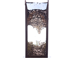
In order to motivate our study, we begin with a specific application. Silicon is commonly produced in submerged arc furnaces (Valderhaug & Sletfjerding Reference Valderhaug and Sletfjerding1991; Valderhaug Reference Valderhaug1992; Schei, Tuset & Tveit Reference Schei, Tuset and Tveit1998; Sloman et al. Reference Sloman, Please, Van Gorder, Valderhaug, Birkeland and Wegge2017), where the oxidisation of quartz rock (SiO $_2$) by lumps of carbon is driven by the heat from electrodes (Halvorsen, Schei & Downing Reference Halvorsen, Schei and Downing1992; Schei et al. Reference Schei, Tuset and Tveit1998; Myrhaug, Tuset & Tveit Reference Myrhaug, Tuset and Tveit2004; Kadkhodabeigi, Tveit & Johansen Reference Kadkhodabeigi, Tveit and Johansen2011). Raw materials are continually added to the top of the furnace to balance the average rate at which material is consumed, with the resulting molten silicon produced then collecting in a pool, before eventually being drained and allowed to solidify (Benham et al. Reference Benham, Hildal, Please and Van Gorder2016a,Reference Benham, Hildal, Please and Van Gorderb; Brosa Planella, Please & Van Gorder Reference Brosa Planella, Please and Van Gorder2019). The mix of solid and granular material above the pool is called the furnace charge. A solid and viscous liquid blockage, known as furnace crust, can build up at the base of the charge (Sloman et al. Reference Sloman, Please, Van Gorder, Valderhaug, Birkeland and Wegge2017; Sloman, Please & Van Gorder Reference Sloman, Please and Van Gorder2018). This crust forms a ceiling-like structure above the pool, creating a cavity containing just gas where no solids or liquids are present. This crust zone is constantly losing material from its lower surface, due to melting and dripping caused by radiative heating from below, but is simultaneously replenished at its upper surface as the granular raw materials melt and stick together, behaving as a highly viscous fluid. Since the crust can resist the raw materials from reaching the hot lower part of the furnace where the dominant reactions occur, it can adversely influence the production of silicon, and as a result the crust has to be broken up with machinery on an hourly basis. This breaking up of the crust is dangerous to operators due to the pressurised hot gas in the furnace, which can flow out uncontrollably once the crust is broken. It is worth noting that silicon is also commonly produced with iron content as ferrosilicon, and when the iron content is high the process does not have the same problematic crust formation (Ksiazek, Tangstad & Ringdalen Reference Ksiazek, Tangstad and Ringdalen2016), possibly due to the added weight of the iron and the lower viscosity of the crust. We examine these hypotheses by developing a thermo-mechanical model of furnace crust, using the simplified cylindrical geometry of experimental furnaces used by Elkem ASA, known as ‘pilot furnaces’ (Sloman et al. Reference Sloman, Please, Van Gorder, Valderhaug, Birkeland and Wegge2017). Annotated images of pilot furnace experiments are shown in figure 1. Since our model generalises the features of furnace crust we anticipate that it will be useful for other applications where a mixture of flow, heating, viscosity changes and material loss occur.

Figure 1. Image of pilot furnace experiment, with (left) and without (right) epoxy injected to take the place of the gas cavity. Note in the experiments the bottom region indicated fallen material will contain some solids that started there. However, in industrial furnaces this will be comprised almost entirely of fallen material.
The charge consists of two regions: an upper region of solid particles, behaving like a granular material, and a lower region comprising a mixture of solid and viscous liquid materials, which are reacting with each other and a background gas. A detailed model of both viscous and granular effects could be excessively complex so, since the highly viscous crust is our main region of interest, it is reasonable to choose a viscous rather than granular modelling framework. For simplicity, we model the lower region as a one-phase viscous liquid, with viscosity dependent on temperature. Granular bridging in the upper charge has not been observed in either industrial or pilot furnaces, likely because the friction coefficient between the walls and the grains is small. Since the solid particles in the upper charge fall down into the space below, we neglect any solid friction between particles and model the granular region as a region of hydrostatic pressure with no horizontal motion of particles. Thus, the upper charge region acts like a dead load, applying pressure to the lower region. This simplification of granular dynamics is taken, since our motivation is to better understand the crust behaviour. In industrial operation raw materials are continually added to keep the top surface as flat as possible, so we assume a fixed top of our granular region. We also ignore the influence of the background gas and any reactions that might create or remove material within the lower charge region. A similar physical configuration has been considered by Ceseri & Stockie (Reference Ceseri and Stockie2014), where a horizontal cylinder comprises three ordered regions of gas, liquid, and solid, respectively. In their paper heating from the gas influences a Stefan condition at the gas–liquid interface, and a long, thin limit is considered.
There have been a variety of studies on the flow and subsequent dripping of a viscous fluid within a vertical tube or similarly confined geometry. A one-dimensional theory of the unsteady extension of a viscous thread under its own weight is derived by Wilson (Reference Wilson1988), and this model holds when viscosity, capillarity and gravity are important but inertia is negligible. Drop formation from a capillary tube for two-phase low Reynolds number flows in a cylindrical geometry was later studied through simulations by Zhang & Stone (Reference Zhang and Stone1997). Tuck, Stokes & Schwartz (Reference Tuck, Stokes and Schwartz1997) model an initially rectangular viscous liquid held fixed between two vertical walls. In the tall, thin limit the profile is parabolic, but is parabolic squared (or quartic shaped) in the short, wide limit. The transition from slow dripping to a jet has been considered by Clanet & Lasheras (Reference Clanet and Lasheras1999), with this transition corresponding to a critical Weber number defined in terms of Bond numbers. Stokes, Tuck & Schwartz (Reference Stokes, Tuck and Schwartz2000) then consider the extensional flow of a viscous fluid forming a droplet. They find a critical ‘crisis time’ at which break-off of a droplet occurs (when inertial effects are neglected). Although it is common to neglect inertia in such flows, the role of inertia in problems of viscous drop formation was considered in Stokes & Tuck (Reference Stokes and Tuck2004).
We are interested in the interactions between thermal effects and flow of the furnace charge. The charge moves under gravity, subject to radiative heating below, from the base of the furnace. In the present paper, we consider the flow of a solid material fed into a vertical tube which melts and flows (as a liquid with strong viscosity dependence on temperature) downward with increasing temperature. There are a variety of scenarios for which this would occur. Natural applications include convection of planetary mantles (Fowler Reference Fowler1985), planetary core formation (Ockendon et al. Reference Ockendon, Tayler, Emerman and Turcotte1985), the dynamics of ice sheet flows (Fowler Reference Fowler1992) and the melting of thin films (Zippelius, Halperin & Nelson Reference Zippelius, Halperin and Nelson1980). Industrial applications include the manufacture of glass and optical fibre, with related models applied to the flow of molten glass (Stokes Reference Stokes1998; Griffiths & Howell Reference Griffiths and Howell2008), the pulling of a hollow glass tube that is being radiatively heated (Huang et al. Reference Huang, Wylie, Miura and Howell2007) and the fabrication of microstructured optical fibres (Tronnolone et al. Reference Tronnolone, Stokes, Foo and Ebendorff-Heidepriem2016; Mavroyiakoumou, Griffiths & Howell Reference Mavroyiakoumou, Griffiths and Howell2019). The winterisation of biodiesel at temperatures below 273 K involves heating of a solid back to a liquid before the biodiesel can be used, and the temperature-dependent viscosity of biodiesel was described by Kerschbaum & Rinke (Reference Kerschbaum and Rinke2004). In most of these applications, there is a melting from solid to liquid phase. Extensional flow of viscous threads was considered by Wylie & Huang (Reference Wylie and Huang2007). Our primary motivating example, however, will be the dynamics found within submerged arc furnaces used in the production of silicon, and in that case the flow is driven by radiative heating from the bottom. For such a configuration, due to continual heating, the viscosity will decrease further until a critical value, after which the fluid drips. This results in three regions: at the top a cool hydrostatic region (granular), then in the middle a warm, highly viscous liquid region (crust), and finally a hot gas-filled region into which the liquid drips (cavity).
At the top of the crust gas condenses, causing particles to stick together, and quartz particles begin to soften and melt. The bottom of the crust is heated from below and the behaviour here is more complex. The mixture can become so hot that there is frequent dripping to the pool below, gas can react with silicon carbide to form low-viscosity silicon and viscous quartz can react with solid carbon and silicon carbide to form gas (Schei et al. Reference Schei, Tuset and Tveit1998; Sloman et al. Reference Sloman, Please, Van Gorder, Valderhaug, Birkeland and Wegge2017). The interface is not smooth, and there can be hanging filaments of material which will drip off. Since we develop a fluid dynamics model motivated by silicon furnaces, rather than attempting to replicate all physical effects observed, we treat both interfaces as isotherms for simplicity. The granular-viscous isotherm represents a condensation temperature, and the viscous-gas isotherm represents a dripping temperature. The energy balance at the lower interface is given by a Stefan condition, with latent heat corresponding to chemical reactions or vaporisation, such as found in the application of liquid flowing through hot porous rock (Woods & Fitzgerald Reference Woods and Fitzgerald1993; Woods Reference Woods1999). We neglect the effect of surface tension, which may influence the detailed shape of the boundary.
There is a wealth of literature concerning temperature-dependent fluid mechanics problems. For example, Ockendon & Ockendon (Reference Ockendon and Ockendon1977) consider a channel of Newtonian fluid that is instantaneously heated or cooled from the walls. A Cartesian channel is assumed, but results are also given for an axisymmetric cylindrical channel. Pearson (Reference Pearson1977) also considers a channel heated from the wall with viscosity having an exponential dependence on temperature. Bergstrøm et al. (Reference Bergstrøm, Cowley, Fowler and Seward1989) and Fitt & Howell (Reference Fitt and Howell1998) analyse two-phase flow with thermally dependent viscosity in furnace electrodes, which is similar to our application of interest. The problem of a warm liquid flowing over a cold semi-infinite solid is examined by Huppert (Reference Huppert1989), with freezing of the liquid and melting of the solid both possible. Further asymptotic limits of this model are studied by King & Riley (Reference King and Riley2000). Models of a similar flavour can also be used to describe problems in application areas such as volcanic eruptions and lava flows (Wylie & Lister Reference Wylie and Lister1995; Lister & Dellar Reference Lister and Dellar1996; Griffiths Reference Griffiths2000), welding (Dowden, Davis & Kapadia Reference Dowden, Davis and Kapadia1983) and fusion reactors (Hassanein, Kulcinski & Wolfer Reference Hassanein, Kulcinski and Wolfer1984).
There are several means of modelling variations in viscosity, with the dependence of viscosity on temperature discussed by several authors (Ockendon & Ockendon Reference Ockendon and Ockendon1977; Pearson Reference Pearson1977; Solomatov Reference Solomatov1995; Wylie & Lister Reference Wylie and Lister1995). The dependence of viscosity on temperature is most often considered to be either exponential ( $\textrm {e}^{-\beta T}$) or algebraic (
 $1-\beta T$) in nature. The exponential decrease of viscosity with temperature is alternately referred to as Reynold's law (Myers, Charpin & Tshehla Reference Myers, Charpin and Tshehla2006) or Nahme's law (Becker & McKinley Reference Becker and McKinley2000; Myers et al. Reference Myers, Charpin and Tshehla2006) in the literature. A variety of studies employ such an exponential dependence of viscosity on temperature (Joseph Reference Joseph1964; Ockendon & Ockendon Reference Ockendon and Ockendon1977; Pearson Reference Pearson1977; Ockendon Reference Ockendon1979; Costa & Macedonio Reference Costa and Macedonio2005), and this will be a sensible choice for our application for silicon furnaces. The situation where the fluid carries a suspension of solid particles has also been well studied (Brinkman Reference Brinkman1952; Chong, Christiansen & Baer Reference Chong, Christiansen and Baer1971; Mueller, Llewellin & Mader Reference Mueller, Llewellin and Mader2009; Mader, Llewellin & Mueller Reference Mader, Llewellin and Mueller2013). A dense suspension limit is examined by Stickel & Powell (Reference Stickel and Powell2005), with Chang & Powell (Reference Chang and Powell1994) studying the influence of the particle size on the rheology. In the furnace crust the solid volume fraction is sufficiently small that variations in the size influence viscosity by orders of magnitude less than variations in temperature. This is shown by noting that the solid particles in the crust have approximately twice the concentration as the viscous quartz (SiO
 $_2$), due to the overall furnace reaction
  $\textrm {SiO}_2+2\textrm {C}\to \textrm {Si}+2\textrm {CO}$ (Schei et al. Reference Schei, Tuset and Tveit1998), and convert to solid silicon carbide particles through the reaction
  $\textrm {SiO}+2\textrm {C}\to \textrm {SiC}+\textrm {CO}$ (Sloman et al. Reference Sloman, Please, Van Gorder, Valderhaug, Birkeland and Wegge2017). Assuming molar volumes
  $2M_{C}/\rho _{C}=1.06\times 10^{-5}, M_{SiC}/\rho _{SiC}=1.25\times 10^{-5}$(Sloman et al. Reference Sloman, Please, Van Gorder, Valderhaug, Birkeland and Wegge2017) and
  $M_{\textrm {SiO}_2}/\rho _{\textrm {SiO}_2}=6.01\times 10^{-2}/2650=2.27\times 10^{-5}$ m
 $^{3}$ mol
 $^{-1}$ (Pabst & Gregorová Reference Pabst and Gregorová2013), and neglecting the small gas fraction, the granular volume fraction ranges from
  $\phi \sim 0.32$ to
  $\phi \sim 0.36$, which is less than the jamming density
  $\phi =0.65$ used by Stickel & Powell (Reference Stickel and Powell2005), and means that changes in solid volume fraction will likely have less influence than changes in temperature on the viscosity. As pointed out by Fitt & Aitchison (Reference Fitt and Aitchison1993) for the related problem of the melting and baking of carbon paste, although such carbon paste is really a two-phase mixture, there is strong industrial interest in treating the paste as a single phase for tractability of models, and therefore an effective viscosity for the whole mixture is desired. Therefore, although the crust likely exhibits non-Newtonian behaviour, we take a similar point of view, treating this region as a homogeneous Newtonian fluid.
Aside from silicon furnaces, there are a variety of applications for the heating and dripping of a solid into a liquid within a thin tube, with perhaps the most common modern application related to phase-change materials. Melting of thin tubes of initially solid phase-change materials, such as paraffin, n-eicosane or RT27 (Rubitherm GmbH), which are heated from below, were studied experimentally and numerically in a variety of works (Sparrow & Broadbent Reference Sparrow and Broadbent1982; Jones et al. Reference Jones, Sun, Krishnan and Garimella2006; Shmueli, Ziskind & Letan Reference Shmueli, Ziskind and Letan2010; Bechiri & Mansouri Reference Bechiri and Mansouri2019), with phase-change nanocomposites such as those based on graphene also attracting attention (Das et al. Reference Das, Takata, Kohno and Harish2016). The melting of both pure substances, as well as substances with impurities, has also been considered (Sparrow, Gurtcheff & Myrum Reference Sparrow, Gurtcheff and Myrum1986). In all of these applications, the vertical tube geometry strongly influences the melting, compares with horizontal tubes or other configurations (Shmueli et al. Reference Shmueli, Ziskind and Letan2010), and this dependence on geometry can play a role in geometric configurations used for thermal energy storage systems (Liu, Yao & Wu Reference Liu, Yao and Wu2013; Dhaidan & Khodadadi Reference Dhaidan and Khodadadi2015). More detailed numerical analysis of phase-change materials melted by heating a vertical cylinder from below suggests the emergence of a moving solid–liquid phase front, with the role of convection also discussed (Wu & Lacroix Reference Wu and Lacroix1995).
Regarding the dripping of thermoviscous fluids confined within cylindrical tubes, a related application can be found within food science (White, Moggridge & Wilson Reference White, Moggridge and Wilson2008). For such foodstuffs, drainage rates are important to know for maintaining the efficiency of industrial processes. Recently, Ali et al. (Reference Ali, Underwood, Lee and Wilson2016) carried out experiments with different sized tubes in order to determine rates of self-drainage of honey and two Marmite(TM) varieties. In their experimental configuration, additional material was added to the top of the cylinder, preventing air entrainment. Detailed modelling of drop formation was not considered, but instead the net rate of material flow was calculated experimentally, as for such applications knowing the total mass flux over time is of greater industrial relevance than is precise knowledge of drop shape and structure. As honey and Marmite(TM) are strongly thermoviscous Ali et al. (Reference Ali, Underwood, Lee and Wilson2016), it is theoretically possible to employ different thermal profiles in order to enhance the rate of dripping (subject to keeping the temperature within a range that prevents spoilage).
Despite the experimental findings and numerical simulations related to applications involving areas as diverse as silicon furnaces, phase-change materials, and melting ice, there is not much work in the literature related to the analysis of such configurations. Motivated by the aforementioned applications, as well as the literature on thermoviscous fluids, in § 2 we develop a two-dimensional axisymmetric model for the flow of a material which melts and then drips. In § 3, we simplify this model by assuming a tall, thin geometry, akin to what is commonly seen in real-world applications. In § 4 we consider steady-state behaviour and perform an asymptotic analysis of the tall, thin geometry model in a variety of physically relevant distinguished limits. We perform numerical simulations of the model in § 5, and in § 6 discuss our results and possible extensions to our work.
2. Thermally driven dripping of a highly viscous fluid in a cylinder
We use an axisymmetric cylindrical geometry, with coordinate system  $(r,z)$, where
  $r$ is the radius and
  $z$ is the height. We do not model the base of the cylinder so consider the semi-infinite region
  $z\leq 0$. We model the crust as a one-phase viscous fluid, with viscosity dependent on temperature. The viscous crust lies above the cavity where there is constant gas pressure and no fluid and the free boundary, at
  $z=-a(r,t)$, separates these regions, where we assume
  $a(r,t)\geq 0$. The movement and shape of this interface will be influenced by the viscous motion of the fluid and thermal heating, and is modelled as a dripping isotherm. We model the granular upper region as a region of hydrostatic pressure with no horizontal motion of particles. This acts like a dead load, applying pressure to the viscous crust below. The granular and viscous regions are separated by the interface
  $z=-b(r,t)$, where we assume
  $0\leq b(r,t)\leq a(r,t)$. This will also be determined by an isotherm, replicating a condensation temperature. We have chosen not to track the behaviour of the material that drips from the viscous crust, and so
  $a(r,t)$ and
  $b(r,t)$ can grow unboundedly. We suppose that material is added to the top of the granular region at a rate which ensures a flat, horizontal top at
  $z=0$, and so only need to consider two free boundaries. A schematic of the geometry is given in figure 2.

Figure 2. A schematic of the two-dimensional geometry, with moving interfaces at  $z=-a(r,t)$ and
  $z=-b(r,t)$, which both have initial conditions
  $a(r,0)=b(r,0)=h$. The temperature of the heat source beneath the fluid is
  $T_h$, the lower and upper fluid interfaces are at isotherms
  $T_d$ and
  $T_k$, respectively, and the top of the domain is at the cold temperature
  $T_c$, where
  $T_c \leq T_k \leq T_d \leq T_h$.
The viscous fluid in  $-a(r,t) \leq z \leq -b(r,t)$ has a Reynolds number such that the Stokes equations hold. The fluid is taken to have a constant density,
  $\rho$, but a thermally varying viscosity,
  $\eta$, so that
 \begin{gather} 0=-\boldsymbol{\nabla} p + \boldsymbol{\nabla} \boldsymbol{\cdot} (\eta ( \boldsymbol{\nabla} \boldsymbol{u}+\boldsymbol{\nabla} \boldsymbol{u}^{T}) ) - \rho g \boldsymbol{k}, \quad \mbox{for } -a(r,t) \leq z \leq -b(r,t), \ r\leq R, \end{gather}
 \begin{gather}\boldsymbol{\nabla} \boldsymbol{\cdot} \boldsymbol{u}=0, \quad \mbox{for } -a(r,t) \leq z \leq -b(r,t), \ r\leq R, \end{gather}
where  $\boldsymbol{u}$ denotes the velocity field and g denotes the acceleration due to gravity. The pressure in the granular region
  $-b(r,t) \leq z \leq 0$ is given by
 \begin{equation} p=p_{atm}-\rho gz, \quad \mbox{for } -b(r,t) \leq z \leq 0, \end{equation}
with no shear stresses and where we have assumed that the granular region has same constant density,  $\rho$, as the fluid region. The flow in this region is assumed to be purely vertical and independent of height. We have continuity of velocity at the interface
  $z=-b(r,t)$, giving
 \begin{equation} \boldsymbol{u}(z,r,t)=\boldsymbol{u}(-b(r,t),r,t), \quad \mbox{for } -b(r,t) \leq z \leq 0, \ r\leq R. \end{equation}
and also continuity of normal and tangential stresses (which we describe in detail later).
We assume that both the viscous and granular regions can be described by the temperature,  $T(r,z,t)$, and the same constant thermal conductivity,
  $k$. Since we neglect any heat from reactions, the governing equation is
 \begin{equation} \frac{\partial T}{\partial t}+\boldsymbol{u} \boldsymbol{\cdot} \boldsymbol{\nabla} T=\kappa \nabla^{2} T, \quad \mbox{for } -a(r,t) \leq z \leq 0, \ r\leq R, \end{equation}
where we have written the convective term as  $\boldsymbol {u} \boldsymbol{\cdot} \boldsymbol {\nabla } T$ due to incompressibility. Since the problem is axisymmetric, we have that
 \begin{equation} T=T(r,z,t), \quad \boldsymbol{u}(r,z,t)=u_r(r,z,t) \boldsymbol{e}_r + u_z(r,z,t) \boldsymbol{k}, \end{equation}
where  $\boldsymbol{e}_r$ denotes the unit vector in the r (radial) direction.
We will solve the fluid problem for  $\boldsymbol {u}$ in the viscous region
  $-a(r,t) \leq z \leq -b(r,t)$, but the thermal problem in the whole fluid domain
  $-a(r,t) \leq z \leq 0$.
The boundary conditions for the viscous fluid are that there is no flux or slip on the radial walls,
 \begin{equation} u_r=0, \quad u_z=0, \quad \mbox{at } r=R, \end{equation}
and that velocity is bounded at  $r=0$,
 \begin{equation} \|\boldsymbol{u}\| \mbox{ bounded as } r\to 0. \end{equation}
We further assume that the cylinder is insulated at the walls and that temperature is bounded along the centreline, so we have
 \begin{equation} \frac{\partial T}{\partial r}=0 \mbox{ at } r=R, \quad T \mbox{ bounded as } r \to 0.\end{equation}
We assume that the top is replenished with cold material,
 \begin{equation} T=T_c, \quad \mbox{at } z=0, \end{equation}
and that the interface  $z=-b(r,t)$ is determined by the condensation isotherm
 \begin{equation} T=T_k, \quad \mbox{at } z=-b(r,t). \end{equation}
The material starts from cold, so we have the initial condition
 \begin{equation} T=T_c, \quad \mbox{at } t=0. \end{equation}
 The behaviour at the lower interface,  $z=-a(r,t)$, is more complex. We have not included a heat source as part of the heat equation (2.5), but energy radiates from the base of the cylinder to cause the lower charge to drip down to the pool below. We thus assume that there is a radiative heat source of constant temperature
  $T_h$ at
  $z=-\infty$. We choose to model the interface
  $z=-a(r,t)$ as an isotherm, corresponding to the temperature at which the fluid drops off instead of staying as a coherent mixture on the time scale of interest. We use the boundary condition
 \begin{equation} T=T_d, \quad \mbox{at } z=-a(r,t), \end{equation}
where  $T_d < T_h$ is the ‘dripping temperature’. There is a natural time scale over which the fluid will viscously deform into drops, and for there to be a stable boundary at the isotherm corresponding to
  $T=T_d$ this time scale should be much less than the time scale over which the temperature of the fluid is changing. As we later see through asymptotic approximations and numerical simulations, parameter values for which the dripping isotherm remains at a fixed height result in a thermal solution which quickly tends to steady state, and therefore heating of the fluid occurs with the slow rate of downward motion. In this case, the time scale for drop formation is much less than the time scale on which the temperature of a given volume element of fluid changes. In the opposite case, where the fluid moves fast enough so that heating of a given volume element is rapid, drops cannot form fast enough, and there is no such stable boundary. Rather, in this regime the dripping isotherm does not occur at steady state, and the fluid is in free fall. We observe both cases, and find that it is the balance between the Stefan and Péclet numbers which dictates whether there is either a stable dripping isotherm or the fluid is in free fall.
To describe the motion of the interface, we use the Stefan condition for convecting material, which is given by
 \begin{equation} \rho L (V_n -\boldsymbol{u}\boldsymbol{\cdot}\boldsymbol{n})=[\boldsymbol{q}\boldsymbol{\cdot} \boldsymbol{n}]^{+}_{-}, \quad \mbox{at } z=-a(r,t).\end{equation}
Here  $\boldsymbol {q}$ is the heat flux,
  $V_n$ is the normal velocity of the interface,
  $\boldsymbol {n}$ is the normal vector to the boundary and
  $L$ is the latent heat of vaporisation, since some of the fluid will be vaporised instead of dripping. Terms on the left-hand side correspond to the interface moving upwards and the fluid moving downwards. The special limit
  $L \to 0$ where no latent heat is given off is considered later in § 4.2.4.
Returning to (2.14), we note that  $V_n$ is given by (see Ockendon et al. Reference Ockendon, Howison, Lacey and Movchan2003)
 \begin{equation} V_n=-\frac{1}{\|\boldsymbol{\nabla} a \|}\frac{\partial (-a)}{\partial t}, \end{equation}
and that the outward normal to the boundary from the fluid is
 \begin{equation} \boldsymbol{n}=\frac{\boldsymbol{\nabla} (-a)}{\|\boldsymbol{\nabla} a \|} =-\frac{1}{\sqrt{1+\left(\dfrac{\partial a}{\partial r}\right)^{2}}}\begin{pmatrix} \dfrac{\partial a}{\partial r}\\ 1 \end{pmatrix}.\end{equation}
Taking care of the signs of the normals for the radiative and conductive fluxes on the right-hand side of (2.16), we obtain
 \begin{align} \rho L \left(\frac{1}{\|\boldsymbol{\nabla} a \|}\frac{\partial (-a)}{\partial t} +\boldsymbol{u}\boldsymbol{\cdot}\frac{\boldsymbol{\nabla} (-a)}{\|\boldsymbol{\nabla} a \|}\right)=-k \boldsymbol{\nabla} T \boldsymbol{\cdot} \boldsymbol{n}-\epsilon_R \sigma ({T_h}^{4}-T_d^{4}) \boldsymbol{k}\boldsymbol{\cdot} \boldsymbol{n}, \quad \mbox{at } z=-a(r,t), \end{align}
for  $\boldsymbol {n}$ given by (2.16), latent heat
  $L$ [m
 $^{-2}$s
 $^{-2}$], emissivity
  $\epsilon _R$ (to avoid confusion with
  $\epsilon$ in § 4.2) and Stefan–Boltzmann constant
  $\sigma$ [kg K
 $^{-4}$ s
 $^{-3}$]. The first term on the right-hand side is the conductive flux lost from the surface, and the second term is the radiative flux from the hot heat source to the surface. We can thus multiply through by
  $\| \boldsymbol {\nabla } a \|$, giving
 \begin{align} \rho L \left(-\frac{\partial a}{\partial t} - u_r \frac{\partial a}{\partial r}-u_z\right)=k\left(\frac{\partial T}{\partial r}\frac{\partial a}{\partial r}+\frac{\partial T}{\partial z}\right)+\epsilon_R \sigma (T_h^{4}-T_d^{4}), \quad \mbox{at } z=-a(r,t). \end{align}
Note that (2.17) includes a simplified radiative flux. More precisely we might account for radiative contributions from each point of the surface of the cavity, however, to do this consistently makes the model inaccessible to analytical progress so we assume a simple heat source radiating at temperature  $T_h$ from
  $z=-\infty$.
At the  $z=-a(r,t)$ boundary, we have that the normal stress is equal to the atmospheric pressure in the gas. In practice there may be some over-pressure in
  $z < - a(r,t)$, but this is not included in our model. We also have that the tangential component of stress is zero. These conditions can be written
 \begin{gather} \boldsymbol{n}\boldsymbol{\cdot} \varSigma \boldsymbol{n}=-p_{atm}, \quad \mbox{at } z=-a(r,t), \end{gather}
 \begin{gather}\quad \boldsymbol{t}\boldsymbol{\cdot} \varSigma \boldsymbol{n}=0, \quad \mbox{at } z=-a(r,t), \end{gather}
for stress tensor,  $\varSigma$, normal vector,
  $\boldsymbol {n}$, and tangent vector,
  $\boldsymbol {t}$. Angular terms do not contribute, so we only give the relevant terms in the tensor
 \begin{equation} \varSigma =\begin{bmatrix} \varSigma_{rr} & \varSigma_{rz} \\ \varSigma_{zr} & \varSigma_{zz} \end{bmatrix} =\begin{bmatrix} -p+2\eta \dfrac{\partial u_r}{\partial r} & \eta \left( \dfrac{\partial u_r}{\partial z} + \dfrac{\partial u_z}{\partial r} \right) \\ \eta \left( \dfrac{\partial u_r}{\partial z} + \dfrac{\partial u_z}{\partial r} \right) & -p+2\eta \dfrac{\partial u_z}{\partial z} \end{bmatrix}. \end{equation}
Since the tangent vector is given by
 \begin{equation} \boldsymbol{t}=\frac{1}{\sqrt{1+\left(\dfrac{\partial a}{\partial r}\right)^{2}}}\begin{pmatrix} 1 \\ -\dfrac{\partial a}{\partial r} \end{pmatrix}, \end{equation}
and noting that  $\varSigma _{rz}=\varSigma _{zr}$, we obtain
 \begin{gather} \frac{1}{1+\left( \dfrac{\partial a}{\partial r}\right)^{2}}\left[\varSigma_{rr} \left(\frac{\partial a}{\partial r} \right)^{2} +2 \varSigma_{rz}\frac{\partial a}{\partial r}+\varSigma_{zz}\right]=-p_{atm}, \quad \mbox{at } z=-a(r,t), \end{gather}
 \begin{gather}\frac{1}{1+\left( \dfrac{\partial a}{\partial r}\right)^{2}}\left[-\varSigma_{rr} \frac{\partial a}{\partial r}-\varSigma_{rz}\left(1-\left( \frac{\partial a}{\partial r}\right)^{2} \right)+ \varSigma_{zz}\frac{\partial a}{\partial r}\right]=0, \quad \mbox{at } z=-a(r,t). \end{gather}
 As mentioned earlier, at  $z=-b(r,t)$, we have analogous conditions arising from continuity of normal and tangential stress. The normal stress is equal to the hydrostatic pressure in the upper region, and the tangential stress is zero. Defining
  $\boldsymbol {n_b}$ and
  $\boldsymbol {t_b}$ as
 \begin{gather} \boldsymbol{n_b}=\frac{1}{\sqrt{1+\left(\dfrac{\partial b}{\partial r}\right)^{2}}}\begin{pmatrix} \dfrac{\partial b}{\partial r}\\ 1 \end{pmatrix}, \end{gather}
 \begin{gather}\boldsymbol{t_b}=\frac{1}{\sqrt{1+\left(\dfrac{\partial b}{\partial r}\right)^{2}}}\begin{pmatrix} 1 \\ -\dfrac{\partial b}{\partial r} \end{pmatrix}, \end{gather}
respectively, we write the stress conditions as
 \begin{gather} \boldsymbol{n_b}\boldsymbol{\cdot} \varSigma \boldsymbol{n_b}=-p_{atm}-\rho g b(r,t), \quad \mbox{at } z=- b(r,t), \end{gather}
 \begin{gather}\boldsymbol{t_b}\boldsymbol{\cdot} \varSigma \boldsymbol{n_b}=0, \quad \mbox{at } z=- b(r,t). \end{gather}
 We assume that the free surfaces start at a given height  $z=-h$, so we have initial conditions
 \begin{equation} a(r,0)=h, \quad b(r,0)=h. \end{equation}
We are aware that this introduces a singularity into the problem, since the viscous region is non-existent initially. However, this is the case in experiments, and later in § 5 we find that a viscous region develops naturally in numerical simulations.
To close the system, we need a constitutive relationship between viscosity and temperature and, since an exponential function is typically used (Ockendon & Ockendon Reference Ockendon and Ockendon1977; Pearson Reference Pearson1977), we set
 \begin{equation} \eta=\eta_s \exp(-\lambda_s(T-T_d)),\end{equation}
for positive parameter  $\eta _s$ and non-negative parameter
  $\lambda _s$.
Our system is thus comprised of (2.1), (2.2), (2.5), boundary conditions (2.4), (2.7a,b)–(2.10), (2.13), (2.23), (2.24), (2.26), initial conditions (2.12) and (2.27), interface conditions (2.11) and (2.18) and the viscosity relationship (2.28).
3. Derivation of the tall, thin cylinder model
We now non-dimensionalise our system under the assumption that the cylinder is tall and thin. We introduce the aspect ratio  $\delta =R/h$, giving the ratio of radial to vertical length scales, and assume that
  $\delta$ is a small parameter with
  $0< \delta \ll 1$. We introduce the scalings
 \begin{equation} \left.\begin{array}{c@{}} u_r=\delta U \bar{u}_r, \quad u_z = U \bar{u}_z, \quad r= \delta h \bar{r}, \quad z=h \bar{z}, \quad a=h\bar{a}, \quad b=h\bar{b}, \\ p =p_{atm}+\dfrac{U \eta_s}{\delta^{2} h} \bar{p}, \quad \eta=\eta_s \bar{\eta}, \quad T=T_c+(T_d-T_c)\bar{T}, \quad t=\dfrac{\rho L h^{2}}{k(T_d-T_c)}\bar{t}, \end{array}\right\} \end{equation}
where we have chosen the Stefan time scale balancing the movement of the interface with the conductive heat flux from the fluid. For the velocity scale we have taken the average speed for Poiseuille flow due to gravity in a cylinder of radius  $R$ for a fluid of constant viscosity
  $\eta _s$, namely
  $U=({\rho g}/{8 \eta _s})R^{2}$.
We find that the leading-order system, as  $\delta \to 0$, will depend on the dimensionless parameters
 \begin{equation} \left. \begin{array}{c@{}} St=\dfrac{C_p (T_d-T_c)}{L}, \quad Pe=\dfrac{U h}{\kappa}, \quad \gamma=\dfrac{\epsilon_R \sigma (T_h^{4}-T_d^{4})}{k(T_d-T_c)/h}, \\ T_b=\dfrac{T_k - T_c}{T_d - T_c}, \quad \lambda=\lambda_s (T_d-T_c). \end{array}\right\}\end{equation}
The Stefan number,  $St$, measures the ratio of sensible heat to latent heat, the thermal Péclet number,
  $Pe$, measures the ratio of the rate of thermal convection to the rate of thermal conduction and the parameter
  $\gamma$ is the ratio of radiative to convective thermal fluxes;
  $T_b$ represents the condensation temperature and
  $\lambda$ the sensitivity of the viscosity to temperature variations. As we examine the problem in the small
  $\delta$ limit, so that the problem domain is a long and thin cylinder, we will treat
  $St, Pe, \gamma , T_b$, and
  $\lambda$ as
  ${O}(1)$ parameters.
Regarding the furnace application, while the latent heat of the mixture is uncertain, for quartz rock the latent heat of vaporisation is  $L=1.56\times 10^{5}$ [J kg
 $^{-1}$] and the corresponding specific heat capacity is
  $C_p = 1.23\times 10^{3}$ [J (kg K)
 $^{-1}$], both calculated from values in Richet et al. (Reference Richet, Bottinga, Denielou, Petitet and Tequi1982) at 1700 K using the molar mass
  $M_{\textrm {SiO}_2}=6.009\times 10^{-2}$ kg mol
 $^{-1}$. A typical difference between the dripping temperature
  $T_d$ and the cold temperature
  $T_c$ at which material enters the furnace is
  $T_d - T_c \sim 1000$ K, which gives an estimate of the Stefan number as
  $St \sim 8$. However, this is a rough estimate, and the Stefan number will be small, order one, or large, depending on particular parameter values, including the temperature difference
  $T_d - T_c$. We will explore these and other scalings in § 4.
For convenience from hereon we drop the overbar notation in (3.1), and obtain the system
 \begin{gather} \frac{\partial u_z}{\partial z}+\frac{1}{r}\frac{\partial}{\partial r}\left(r u_r \right)=0, \end{gather}
 \begin{gather}0=-\frac{\partial p}{\partial z}+\frac{1}{r}\frac{\partial}{\partial r} \left(r \eta \frac{\partial u_z}{\partial r} \right)-8+{O}(\delta^{2}), \end{gather}
 \begin{gather}0=-\frac{\partial p}{\partial r}+{O}(\delta^{2}), \end{gather}
 \begin{gather}\frac{\partial T}{\partial t}+\frac{Pe}{St} \left(u_r\frac{\partial T}{\partial r}+u_z \frac{\partial T}{\partial z}\right)=\frac{1}{St} \left( \frac{1}{\delta^{2}}\frac{1}{r}\frac{\partial}{\partial r}\left(r \frac{\partial T}{\partial r} \right) +\frac{\partial^{2} T}{\partial z^{2}}\right), \end{gather}
 \begin{gather}\eta=\exp(-\lambda(T-1)). \end{gather}
We have the following boundary and initial conditions
 \begin{gather} T(r,-a(r,t),t)=1, \quad T(r,0,t)=0, \quad \frac{\partial T}{\partial r}(1,z,t)=0, \quad T \mbox{ bounded as } r \to 0, \end{gather}
 \begin{gather}T(r,z,0)=0, \end{gather}
 \begin{gather}u_r(1,z,t)=0, \quad u_z(1,z,t)=0, \quad \|\boldsymbol{u}\| \mbox{ is bounded as } r\to 0. \end{gather}
We note that the atmospheric pressure terms  $p_{atm}$ cancel in both stress conditions (2.23) and (2.24), and hence we find
 \begin{align} &\left(-\frac{p}{\delta^{2}}+2\eta \frac{\partial u_r}{\partial r} \right)\frac{1}{\delta^{2}}\left(\frac{\partial a}{\partial r}\right)^{2} +2\eta \left(\delta \frac{\partial u_r}{\partial z}+\frac{1}{\delta}\frac{\partial u_z}{\partial r}\right)\frac{1}{\delta}\frac{\partial a}{\partial r}\nonumber\\ &\quad-\frac{p}{\delta^{2}}+2\eta \frac{\partial u_z}{\partial z}=0, \quad \mbox{at } z=-a(r,t), \end{align}
 \begin{align} &-\left(-\frac{p}{\delta^{2}}+2\eta\frac{\partial u_r}{\partial r}\right)\frac{1}{\delta}\frac{\partial a}{\partial r}-\eta\left(\delta \frac{\partial u_r}{\partial z}+\frac{1}{\delta}\frac{\partial u_z}{\partial r} \right)\left(1-\frac{1}{\delta^{2}} \left(\frac{\partial a}{\partial r}\right)^{2}\right)\nonumber\\ &\quad +\left(-\frac{p}{\delta^{2}}+2\eta\frac{\partial u_z}{\partial z} \right)\frac{1}{\delta}\frac{\partial a}{\partial r}=0 \quad \mbox{at } z=-a(r,t). \end{align}
Similarly the free stress conditions (2.26) on the upper surface become
 \begin{align} &\left(-\frac{p}{\delta^{2}}+2\eta \frac{\partial u_r}{\partial r} \right)\frac{1}{\delta^{2}}\left(\frac{\partial b}{\partial r}\right)^{2}-2\eta \left(\delta \frac{\partial u_r}{\partial z}+\frac{1}{\delta}\frac{\partial u_z}{\partial r}\right)\frac{1}{\delta}\frac{\partial b}{\partial r}-\frac{p}{\delta^{2}}+2\eta \frac{\partial u_z}{\partial z}\nonumber\\ &\quad =-\frac{8}{\delta^{2}}b(r,t)\left(1+\frac{1}{\delta^{2}}\left(\frac{\partial b}{\partial r} \right)^{2} \right), \quad \mbox{at } z=-b(r,t), \end{align}
 \begin{align} &\left(-\frac{p}{\delta^{2}}+2\eta\frac{\partial u_r}{\partial r}\right)\frac{1}{\delta}\frac{\partial b}{\partial r}+\eta\left(\delta \frac{\partial u_r}{\partial z}+\frac{1}{\delta}\frac{\partial u_z}{\partial r} \right)\left(1-\frac{1}{\delta^{2}} \left(\frac{\partial b}{\partial r}\right)^{2}\right)\nonumber\\ &\quad -\left(-\frac{p}{\delta^{2}}+2\eta\frac{\partial u_z}{\partial z} \right)\frac{1}{\delta}\frac{\partial b}{\partial r}=0, \quad \mbox{at } z=-b(r,t). \end{align}
We also have the interface conditions
 \begin{gather} -\frac{\partial a}{\partial t}-\frac{Pe}{St} \left( u_r \frac{\partial a}{\partial r}+u_z\right)=\gamma + \frac{\partial T}{\partial z}+\frac{1}{\delta^{2}} \frac{\partial T}{\partial r}\frac{\partial a}{\partial r}, \quad \mbox{at } z=-a(r,t), \end{gather}
 \begin{gather}a(0,t)=1, \end{gather}
 \begin{gather}T(-b(r,t),r,t)=T_b, \end{gather}
 \begin{gather}b(0,t)=1. \end{gather}
3.1. Derivation of the leading-order system
Since we have taken a tall, thin limit, we expect that the lower interface is flat to leading order. To demonstrate this, we note that the leading-order terms in (3.3i) and (3.3j) are
 \begin{equation} -p \left( \frac{\partial a}{\partial r}\right)^{2}=0, \quad \eta \frac{\partial u_z}{\partial r}\left( \frac{\partial a}{\partial r}\right)^{2}=0. \end{equation}
If we did not take  ${\partial a}/{\partial r}=0$, then in addition to zero pressure
  $p=0$, we would also need the vertical component of velocity to be radially independent at the interface. Due to the no-flux condition on the wall, this would require zero vertical velocity across the whole interface, and hence throughout the entire fluid region. Thus, since we want to include convection in our model, we must have that the interface is flat to leading order.
Further, letting  $a=a_0(t) + \delta a_1(r,t) +{O}(\delta ^{2})$ we note that the next-order term in (3.3i) is given by
 \begin{equation} -p_0 \left(\frac{\partial a_1}{\partial r} \right)^{2}-p_0=0, \end{equation}
for leading-order pressure  $p_0$. We thus obtain a zero pressure condition on the flat, lower interface
 \begin{equation} p_0=0, \quad \mbox{at } z=-a_0(t). \end{equation}
By similar reasoning with (3.3k) and (3.3l), we also obtain a flat upper interface to leading order, so  $b=b_0(t)+{O}(\delta )$, and we find the pressure condition
 \begin{equation} p_0=8b_0(t), \quad \mbox{at } z=-b_0(t). \end{equation}
 We now expand the temperature, velocity, pressure and viscosity variables. Due to the  $\delta ^{-2}$ term in the heat equation (3.3d), we consider expansions of the form
 \begin{gather} T= T_0 +\delta^{2} T_1 +{O}(\delta^{4}), \end{gather}
 \begin{gather}\boldsymbol{u}=\boldsymbol{u}_0+\delta^{2} \boldsymbol{u}_1 +{O}(\delta^{4}), \end{gather}
 \begin{gather}p=p_{0} +\delta^{2} p_{1} +{O}(\delta^{4}), \end{gather}
 \begin{gather}\eta=\eta_0 + \delta^{2} \eta _1 + {O}(\delta^{4}). \end{gather}
The leading-order thermal equation is
 \begin{equation} 0=\frac{1}{St} \frac{1}{r}\frac{\partial}{\partial r}\left(r \frac{\partial T_0}{\partial r} \right), \end{equation}
which, combined with either the boundedness of  $T_0$ as
  $r \to 0$ or the vanishing normal derivative on the wall
  $r=1$, gives
  $T_0=T_0(z,t)$ (for
  $St={O}(1)$ in
  $\delta$, which we have assumed). This, in turn, gives that the leading-order viscosity is also radially independent, with
 \begin{equation} \eta_0(z,t)=\exp(-\lambda (T_0(z,t)-1) ). \end{equation}
The leading-order fluid equations are
 \begin{gather} \frac{\partial u_{z0}}{\partial z}+\frac{1}{r}\frac{\partial}{\partial r}\left(r u_{r0} \right)=0, \end{gather}
 \begin{gather}0=-\frac{\partial p_{0}}{\partial z}+\frac{1}{r}\frac{\partial}{\partial r} \left(r \eta_0 \frac{\partial u_{z0}}{\partial r} \right)-8, \end{gather}
 \begin{gather}0=-\frac{\partial p_{0}}{\partial r}, \end{gather}
 \begin{gather}u_{r0}(1,z,t)=u_{z0}(1,z,t)=0, \end{gather}
 \begin{gather}u_{r0}, \quad u_{z0} \mbox{ bounded as } r\to 0, \end{gather}
 \begin{gather}p_0(r,-a_0(t),t)=0, \quad p(r,-b_0(t),t)=8b_0(t). \end{gather}
Since the leading-order pressure  $p_0$ is also radially independent, (3.11b) can be integrated twice to give
 \begin{equation} u_{z0}=-\frac{1}{\eta_0(z,t)}\left(\frac{\partial p_0}{\partial z}+8 \right)\left(\frac{1-r^{2}}{4} \right). \end{equation}
Integrating the incompressibility condition (3.11a) radially gives
 \begin{equation} \int_{0}^{1} r\frac{\partial u_{z0}}{\partial z}\, \textrm{d} r+[r u_{r0} ]_{r=0}^{r=1}=0. \end{equation}
The boundary conditions on  $u_{r0}$, combined with (3.12), give
 \begin{equation} \frac{\partial}{\partial z}\left( \frac{1}{\eta_0}\left( \frac{\partial p_0}{\partial z}+8\right) \right)=0,\end{equation}
and hence  $u_{z0}$ is independent of height
  $z$. Substituting
  $u_{z0}$ into the incompressibility condition (3.11a), we find that
  $u_{r0}=0$. Thus, to leading order, the fluid moves downward with a velocity that is the same at each height, yet which varies radially and temporally. We have that
 \begin{equation} \boldsymbol{u}_0= -2 f(t)(1-r^{2})\boldsymbol{k}, \end{equation}
where  $f(t)$ can be interpreted as the average speed of the fluid, since
 \begin{equation} \left|\frac{2\pi \displaystyle\int_{r=0}^{1} 2 f(t) (r^{2}-1) r \, \textrm{d} r}{2 \pi \displaystyle\int_{r=0}^{1} r \, \textrm{d} r}\right|=f(t). \end{equation}
We can find  $f(t)$ by substituting (3.15) into (3.11b), which when rearranged gives
 \begin{equation} 8 f(t) \eta_0=8+\frac{\partial p_0}{\partial z}. \end{equation}
Integrating (3.17) vertically between  $z=-a_0(t)$ and
  $z=-b_0(t)$, we have
 \begin{align} 8 f(t) \int_{-a_0(t)}^{-b_0(t)}\eta_0 (z,t) \, \textrm{d} z =[p_0 + 8 z ]_{z=-a_0(t)}^{z=-b_0(t)}=8b_0(t)+8(-b_0(t) + a_0(t)), \end{align}
and hence we obtain
 \begin{equation} f(t)=\frac{a_0(t)}{\displaystyle\int_{z=-a_0(t)}^{-b_0(t)}\eta_0(z,t) \, \textrm{d} z}. \end{equation}
Thus,  $f(t)$ is a ratio of the gravitational force in the numerator driving the fluid downwards to the viscous force in the denominator resisting motion. Note that the weight of the whole charge is felt, but the resistance is due only to the viscosity of the lower region. We note that in the case of constant viscosity (
 $\lambda =0$), and no granular region (
 $T_b=1$), we have that
  $f(t)\equiv 1$, and we recover the usual Poiseuille flow results.
We determine an equation for  $T_0(z,t)$ by considering the
  ${O}(1)$ heat equation, namely
 \begin{equation} \frac{\partial T_0}{\partial t}+\frac{Pe}{St}u_{z0} \frac{\partial T_0}{\partial z}=\frac{1}{St} \left(\frac{1}{r}\frac{\partial}{\partial r}\left(r \frac{\partial T_1}{\partial r} \right) +\frac{\partial^{2} T_0}{\partial z^{2}}\right). \end{equation}
Integrating (3.20) radially, noting that  $T_0$ is independent of
  $r$, gives
 \begin{equation} \frac{1}{2} \frac{\partial T_0}{\partial t}-\frac{1}{2}\frac{Pe}{St} f(t) =\frac{1}{St} \int_{r=0}^{1} \frac{\partial}{\partial r}\left(r \frac{\partial T_1}{\partial r} \right)\, \textrm{d} r +\frac{1}{2}\frac{1}{St}\frac{\partial^{2} T_0}{\partial z^{2}}. \end{equation}
Since  $T_1$ is bounded at
  $r \to 0$ and has a zero normal derivative on the wall
  $r=1$, we are left with
 \begin{equation} \frac{\partial T_0}{\partial t}-\frac{Pe}{St}f(t)\frac{\partial T_0}{\partial z}=\frac{1}{St}\frac{\partial^{2} T_0 }{\partial z^{2}}, \quad \mbox{in } -a_0(t) \leq z \leq 0, \end{equation}
with the corresponding initial and boundary conditions
 \begin{equation} T_0(z,0)=0,\quad T_0(-a_0(t),t)=1, \quad T_0(0,t)=0. \end{equation}
We note that the location of the interface  $z=-b(t)$ is determined by
 \begin{equation} T_0(-b_0(t),t)=T_b. \end{equation}
We also need to determine the leading-order Stefan condition. Considering the leading-order terms in (3.3m) gives
 \begin{equation} -\frac{\textrm{d} a_0}{\textrm{d} t}+\frac{Pe}{St} 2f(t)(1-r^{2})=\gamma +\frac{\partial T_0}{\partial z}, \quad \mbox{at } z=-a_0(t), \end{equation}
which cannot be satisfied by the leading-order solution, because  $a_0$ and
  $T_0$ are independent of
  $r$ and
  $f(t) >0$, so nothing can balance the single term with radial dependence. The problem arises because we have shown that the lowest-order interface
  $a_0(t)$ is flat, and that the lowest-order temperature
  $T_0$ is radially independent. However, at higher orders, the interface is not flat, and varies radially. We thus we must consider an inner region adjacent to the interface where temperature could potentially vary radially. We expect this region to be of thickness
  ${O}(\delta )$, and hence in a domain that is not tall and thin. We now consider this boundary region to find that we should impose a radially averaged boundary condition on the lowest-order outer problem.
3.2. Averaged velocity from inner region
We consider the small inner region at the bottom of the lower, viscous region by defining the inner variables  $a_I(r,t), \hat {z}$, and
  $T_I(\hat {z},r,t)$ as
 \begin{equation} a=a_0(t) + \delta a_I(r,t), \quad T=1+\delta T_I(\hat{z},r,t), \quad z=-a_0(t) +\delta \hat{z}, \end{equation}
where  $r, t \geq 0$ and
  $\hat {z} \geq -a_I$. We have assumed that the correction term lies below the leading-order interface, i.e.
  $a_I >0$. A schematic diagram of the inner region is given in figure 3.

Figure 3. Schematic of the inner region near  $z=-a_0(t)$.
The leading-order temperature equation in the inner region is given by
 \begin{equation} \hat{\nabla}^{2} T_I=0, \quad \hat{z} \geq -a_I(r,t), \end{equation}
where the hat on the Laplacian denotes derivatives with respect to  $r$ and
  $\hat {z}$. We have the inner velocity profile,
  $\boldsymbol {u}_I$, which scales with the outer velocity and satisfies the incompressibility condition
  $\hat {\boldsymbol {\nabla }} \boldsymbol{\cdot} \boldsymbol {u}_I=0$.
The leading-order Stefan condition in the inner region is given by
 \begin{equation} -\frac{\textrm{d} a_0(t)}{\textrm{d} t}+\frac{Pe}{St} \boldsymbol{u}_I \boldsymbol{\cdot} \hat{\boldsymbol{\nabla}} (-a_I) =\gamma-\hat{\boldsymbol{\nabla}} T_I \boldsymbol{\cdot} \hat{\boldsymbol{\nabla}}(- a_I), \quad \mbox{at } \hat{z}=-a_I, \end{equation}
or, alternatively, by
 \begin{equation} -\frac{1}{\| \hat{\boldsymbol{\nabla}} (-a_I) \|}\frac{\textrm{d} a_0(t)}{\textrm{d} t}+\frac{Pe}{St} \boldsymbol{u}_I \boldsymbol{\cdot} \boldsymbol{n}_I =\frac{\gamma}{\| \hat{\boldsymbol{\nabla}} (-a_I) \|}-\hat{\boldsymbol{\nabla}} T_I \boldsymbol{\cdot} \boldsymbol{n}_I, \quad \mbox{at } \hat{z}=-a_I, \end{equation}
where we have defined the downwards pointing inner normal  $\boldsymbol {n}_I=\hat {\boldsymbol {\nabla }} (-a_I)/\|\hat {\boldsymbol {\nabla }}(-a_I)\|$. We also have that
 \begin{equation} T_I=0, \quad \mbox{at } \hat{z}=a_I, \quad \frac{\partial T_I}{\partial r}=0=u_{Iz}=u_{Ir}, \quad \mbox{ at } r=1, \end{equation}
and the matching conditions with the leading-order outer variables  $T_0$ and
  $\boldsymbol {u}_0$. Using Van Dyke's matching principle, noting that
  $T_{0z}(-a_0(t) + \delta \hat {z},t) = T_{0z}(-a_0(t),t)+{O}(\delta )$, we have
 \begin{equation} \frac{\partial T_I}{\partial \hat{z}}(\infty,r,t) =\frac{\partial T_0}{\partial z}(-a_0(t),t), \quad \boldsymbol{u}_I(\infty,r,t)=\boldsymbol{u_0}(-a_0(t),t). \end{equation}
 Integrating (3.29) along the surface  $\hat {z}=-a_I(r,t)$, we obtain
 \begin{align} \iint_{\hat{z}=-a_I}\left( - \frac{1}{\| \hat{\boldsymbol{\nabla}} (-a_I) \|}\frac{\textrm{d} a_0(t)}{\textrm{d} t}+\frac{Pe}{St} \boldsymbol{u}_I \boldsymbol{\cdot} \boldsymbol{n}_I \right)\, \textrm{d} S =\iint_{\hat{z}=-a_I} \left(\frac{\gamma}{\| \hat{\boldsymbol{\nabla}} (-a_I) \|}-\hat{\boldsymbol{\nabla}} T_I \boldsymbol{\cdot} \boldsymbol{n}_I \right) \, \textrm{d} S. \end{align}
Using the divergence theorem in the region bounded by  $\hat {z}=a_I, \hat {z}=\infty$ and the cylindrical wall
  $r=1$, and noting that
  $\hat {\nabla }^{2} T_I=0$, we find
 \begin{equation} \iint_{\hat{z}=-a_I}\hat{\boldsymbol{\nabla}} T_I \boldsymbol{\cdot} \boldsymbol{n}_I \, \textrm{d} S = -\iint_{\hat{z}=\infty}\hat{\boldsymbol{\nabla}}T_I \boldsymbol{\cdot} \boldsymbol{k} \, \textrm{d} S. \end{equation}
Since  $\hat {\boldsymbol {\nabla }}T_I \to \boldsymbol {\nabla } T_0 (-a_0(t),t)$ as
  $\hat {z}\to \infty$, we obtain
 \begin{equation} \iint_{\hat{z}=-a_I}\hat{\boldsymbol{\nabla}}T_I \boldsymbol{\cdot} \boldsymbol{n}_I \, \textrm{d} S =-\int_{\theta=0}^{2\pi} \int_{r=0}^{1} r\frac{\partial T_0}{\partial z}(-a_0(t),t) \, \textrm{d} r \, \textrm{d} \theta= -\pi \frac{\partial T_0}{\partial z}(-a_0(t),t). \end{equation}
Similarly, since  $\boldsymbol {u}_I$ is incompressible and there are zero flux conditions on the walls, we can use the divergence theorem to write
 \begin{equation} \iint_{\hat{z}=-a_I}\boldsymbol{u}_I \boldsymbol{\cdot} \boldsymbol{n}_I \, \textrm{d} S =-\iint_{\hat{z}=\infty}\boldsymbol{u}_I \boldsymbol{\cdot} \boldsymbol{k} \, \textrm{d} S = -\int_{\theta=0}^{2\pi} \int_{r=0}^{1} r u_{z0}(-a_0(t),t) \, \textrm{d} r \, \textrm{d} \theta= \pi f(t), \end{equation}
where we have used  $\boldsymbol {u}_0=-2f(t)(1-r^{2})\boldsymbol {k}$ from the outer problem (3.15).
Noting that
 \begin{equation} \iint_{\hat{z}=-a_I} \frac{1}{\| \hat{\boldsymbol{\nabla}}(-a_I) \|} \, \textrm{d} S = \iint_{\hat{z}=-a_I} -\boldsymbol{k}\boldsymbol{\cdot} \boldsymbol{n}_I \, \textrm{d} S = \pi, \end{equation}
is the projected area of the surface onto the plane orthogonal to  $\boldsymbol {k}$, and that
  ${\textrm {d} a_0}/{\textrm {d} t}$ and
  $\gamma$ are constant with respect to the integrals, we find
 \begin{equation} -\frac{\textrm{d} a_0(t)}{\textrm{d} t}+\frac{Pe}{St}f(t)=\gamma + \frac{\partial T_0}{\partial z}, \quad \mbox{at } z=-a_0(t). \end{equation}
Thus our analysis of the inner problem has identified that we should impose a radially averaged boundary condition (3.37), instead of (3.25), on the flat outer position of the interface for the lowest-order outer variables. Equation (3.37) is an averaged Stefan condition and closes the leading-order outer problem.
3.3. Statement of the model for a tall, thin cylinder
We simplify the notation used in the previous sections when we derived the lowest-order behaviour by dropping the  $0$ subscripts, so that the problem we seek to study is given by
 \begin{gather} \frac{\partial T}{\partial t}-\frac{f(t) Pe}{ St}\frac{\partial T}{\partial z}=\frac{1}{St}\frac{\partial^{2} T}{\partial z^{2}},\quad \mbox{for } -a(t) \leq z \leq 0, \end{gather}
 \begin{gather}-\frac{\textrm{d} a}{\textrm{d} t}+\frac{f(t) Pe}{St}=\gamma + \frac{\partial T}{\partial z}, \quad \mbox{at } z=-a(t), \end{gather}
 \begin{gather}T(0,t)=0, \end{gather}
 \begin{gather}T(-b(t),t)=T_b, \end{gather}
 \begin{gather}T(-a(t),t)=1, \end{gather}
 \begin{gather}T(z,0)=0, \end{gather}
 \begin{gather}a(0)=1, \quad b(0)=1, \end{gather}
where
 \begin{equation} f(t)=\frac{a(t)}{\displaystyle\int_{z=-a(t)}^{-b(t)}\exp(-\lambda(T(z,t)-1)) \, \textrm{d} z}. \end{equation}
Upon solving this system for  $T(z,t), a(t), b(t)$ and
  $f(t)$, we may determine the fluid velocity, which is given by
 \begin{equation} \boldsymbol{u}=-2f(t)(1-r^{2})\boldsymbol{k}, \end{equation}
as well as the volumetric flow rate of material across the interface  $z=-a(t)$, which is given by
 \begin{align} Q(t) &= -\int_{\theta=0}^{2\pi} \int_{r=0}^{1}\left(\frac{\textrm{d} a}{\textrm{d} t} -\boldsymbol{u}\boldsymbol{\cdot} \boldsymbol{n}\right) r \, \textrm{d} r \, \textrm{d} \theta \nonumber\\ &= -2\pi \int_{\theta=0}^{\pi} \int_{r=0}^{1} \left( \frac{\textrm{d} a}{\textrm{d} t}-2f(t)(1-r^{2})\right)r \,\mathrm{d}r \nonumber\\ &= \pi\left( f(t)-\frac{\textrm{d} a}{\textrm{d} t}\right). \end{align}
Here we have chosen to define  $Q>0$ in (3.40) when material is dripping from the base of the fluid. A schematic diagram of the tall, thin model is given in figure 4.

Figure 4. Schematic of the problem geometry for the tall, thin cylinder model (3.38). The viscous region (blue) is separated from the granular region (red) above by the isotherm  $T=T_b$ at
  $z=-b(t)$ and is bounded below by the isotherm
  $T=1$ at
  $z=-a(t)$. The top of the granular region is cold,
  $T=0$, and at a fixed height
  $z=0$. The moving boundaries have initial conditions
  $a(0)=b(0)=1$.
4. Steady-state dynamics and asymptotic analysis
In some furnace operations and experiments, the thickness of the crust appears to become steady in time, suggesting that the dynamics of (3.38) tends toward a steady-state solution. In this section, we first analyse the steady states of (3.38) for general parameter values in § 4.1. Later, in § 4.2, we carry out an asymptotic analysis of (3.38) under various distinguished asymptotic limits of the model parameters, in order to better understand the qualitative dependence of these steady-state solutions to (3.38) on these model parameters.
4.1. Steady-state solutions
For our model, we find that steady-state solutions cannot be written in an explicit closed form, but depend upon an implicit equation for  $f$ that arises from (3.38h), which must be solved numerically. We find two roots to this equation, corresponding to two steady states. We show numerical evidence suggesting that one of these steady states is stable, while the other steady state is unstable. Subsequently, in § 5.2, we plot bifurcation diagrams of the model behaviour in parameter space.
Suppose we look for a steady-state solution, so that  $a(t)=a^{*}, b(t)=b^{*}, T(z,t)=T^{*}(z)$ and
  $f(t)=f^{*}$. The system (3.38) then becomes
 \begin{gather} -f^{*} Pe \frac{\textrm{d} T^{*}}{\textrm{d} z} =\frac{\textrm{d}^{2} T^{*}}{\textrm{d} z^{2}}, \quad \mbox{in } -a^{*} \leq z \leq 0, \end{gather}
 \begin{gather}\frac{f^{*} Pe}{St}=\gamma+\frac{\partial T^{*}}{\partial z}, \quad \mbox{at } z=-a^{*}, \end{gather}
 \begin{gather}T^{*}(-a^{*})=1, \quad T^{*}(0)=0, \end{gather}
 \begin{gather}T^{*}(-b^{*})=T_b, \end{gather}
 \begin{gather}f^{*}=\frac{a^{*}}{\displaystyle\int_{z=-a^{*}}^{-b^{*}}\exp\left(-\lambda(T^{*}-1) \right)\, \textrm{d} z}. \end{gather}
The equation (4.1a) combined with the boundary conditions (4.1c) can be solved to find the steady-state temperature profile
 \begin{equation} T^{*}(z)=\frac{\exp(-f^{*}Pe\, z)-1}{\exp(\,f^{*}Pe\, a^{*})-1}. \end{equation}
We can then use the Stefan condition (4.1b) to find an equation for the position of the free boundary, which reads
 \begin{equation} \frac{f^{*} Pe}{ St}=\gamma-f^{*} Pe\frac{\exp(\,f^{*} Pe\, a^{*})}{\exp(\,f^{*} Pe\, a^{*})-1}. \end{equation}
This can be rearranged to determine that the lower interface is at
 \begin{equation} a^{*}=\frac{1}{f^{*} Pe}\ln\left(\frac{\dfrac{\gamma }{f^{*} Pe}-\dfrac{1}{St}}{\dfrac{\gamma }{f^{*} Pe}-\dfrac{1}{St}-1}\right).\end{equation}
We use the isotherm (4.1d) to find that the upper interface is at
 \begin{equation} b^{*}=\frac{1}{f^{*} Pe}\ln(1+T_b(\exp(\,f^{*} Pe\, a^{*})-1 )). \end{equation}
When  $T_b=0$, the upper interface is at the top of the domain (
 $b^{*}=0$). When
  $T_b=1$, we find that (4.5) simplifies to give
  $b^{*}=a^{*}$, which is also expected. Note that we have not yet found
  $a^{*}$ and
  $b^{*}$ explicitly as functions of the parameters
  $Pe, St, \gamma , T_b$, and
  $\lambda$, since (4.4) and (4.5) still have a dependence on
  $f^{*}$. The crucial equation we have not yet used is (4.1e), which we write as the implicit integral equation for
  $f^{*}$
 \begin{equation} f^{*}=\frac{a^{*}}{\displaystyle\int_{z=-a^{*}}^{-b^{*}}\exp\left(-\lambda\left(\frac{\exp\left(-f^{*} Pe\, z\right)-1}{\exp\left(\,f^{*} Pe\, a^{*}\right)-1}-1\right) \right)\, \textrm{d} z}.\end{equation}
We thus seek the solutions  $a^{*}, b^{*}$, and
  $f^{*}$ to the coupled equations (4.4)–(4.6), noting that if we can find
  $f^{*}$ we can subsequently obtain
  $a^{*}$ and
  $b^{*}$ through substitution.
To help solve the problem (4.4)–(4.6) we make the change of variable
 \begin{equation} \theta =\frac{\gamma }{f^{*} Pe}-\frac{1}{St}. \end{equation}
This allows us to write (4.4), (4.5) and (4.6), respectively, as
 \begin{gather} a^{*}=\frac{1}{f^{*}Pe}\ln\left(\frac{\theta}{\theta-1}\right)=\frac{1}{\gamma}\left(\theta+\frac{1}{St} \right)\ln\left(\frac{\theta}{\theta-1}\right), \end{gather}
 \begin{gather}b^{*}=\frac{1}{f^{*}Pe}\ln \left(1+\frac{T_b}{\theta -1} \right)=\frac{1}{\gamma}\left(\theta+\frac{1}{St} \right)\ln \left(1+\frac{T_b}{\theta -1} \right), \end{gather}
 \begin{gather}f^{*} \textrm{e}^{\lambda} \int_{z=-a^{*}}^{-b^{*}}\exp \left(-\lambda (\theta-1) \left(\exp\left(-f^{*} Pe\, z\right)-1 \right) \right)\, \textrm{d} z=\frac{1}{\gamma}\left(\theta+\frac{1}{St} \right)\ln\left(\frac{\theta}{\theta-1}\right). \end{gather}
We now look for the solutions  $a^{*}, b^{*}$ and
  $\theta$ of the system (4.8)–(4.10).
We must take care to ensure the logarithms in (4.8)–(4.10) are well-defined. The parameters  $St, Pe$ and
  $\gamma$ are all positive,
  $T_b \in [0,1]$ and
  $f^{*}$ is non-negative. The logarithm in (4.8) and (4.10) is not well defined for
  $\theta \in [0,1]$. In the case that
  $\theta <0$, we have
  $a^{*}<0$ and thus a steady state at
  $z=-a^{*}$ which is above the top of the domain, which is evidently not physically attainable. The logarithm in (4.9) is not defined for
  $\theta \in [1-T_b,1]$. For
  $\theta <1-T_b$ we have
  $b^{*}<0$, which is also not physically attainable. Hence, we must have
  $\theta >1$ for physically relevant steady states to exist.
We seek to simplify (4.10), by making the substitution
 \begin{equation} w=\lambda(\theta-1)\exp(-f^{*} Pe\, z),\end{equation}
which transforms (4.10) to
 \begin{equation} -\frac{ \textrm{e}^{\lambda \theta}}{Pe} \int_{w=\lambda \theta}^{\lambda(\theta+T_b-1)} \frac{\textrm{e}^{-w} }{w}\, \textrm{d} w=\frac{1}{\gamma}\left(\theta+\frac{1}{St} \right)\ln\left(\frac{\theta}{\theta-1}\right).\end{equation}
Using the exponential integral  $E_1(x)$, given by
 \begin{equation} E_1(x)=\int_{x}^{\infty} \frac{\textrm{e}^{-t}}{t} \, \textrm{d} t, \end{equation}
we can rewrite (4.12) as
 \begin{equation} \textrm{e}^{\lambda \theta}( E_1(\lambda(\theta-1+T_b))-E_1( \lambda \theta) )=\frac{Pe}{\gamma}\left(\theta+\frac{1}{St}\right)\ln\left(\frac{\theta}{\theta-1}\right). \end{equation}
Since there is a one-to-one mapping between  $f^{*}$ and
  $\theta$ (defined in (4.7)), each root of (4.14) for
  $\theta$ corresponds to a steady state
  $f^{*}$. Note also that
  $Pe/\gamma$ acts as one parameter in (4.14), and so there are only four parameter groupings in (4.14), being
  $St, T_b, \lambda$ and
  $Pe/\gamma$. In exploring this parameter regime we recall we require
  $\theta >1$, which implies
  $f^{*} < {\gamma }/{Pe (1+1/St)}$.
Numerical evidence suggests the existence of at most one stable steady state for given parameters, although we shall now show that multiple steady states are possible, with the additional steady state seemingly unstable. We introduce the function
 \begin{equation} \phi(\theta)= \textrm{e}^{\lambda \theta}\left( E_1\left(\lambda(\theta-1+T_b)\right)-E_1\left( \lambda \theta\right) \right)-\frac{Pe}{\gamma}\left(\theta+\frac{1}{St}\right)\ln\left(\frac{\theta}{\theta-1}\right), \end{equation}
so that each zero of (4.15) corresponds to a root of (4.14). If the partial derivatives of  $\phi$ were all single-signed then it could have at most one root. This is true for the derivatives with respect to
  $St, Pe/\gamma$, and
  $T_b$, but unfortunately not for
  $\lambda$ and
  $\theta$. Instead, to determine the number of roots of (4.14), we plot contours of roots of
  $\phi$ for
  $\lambda$ against
  $\theta$, for different values of the other parameters. If the contours are monotonic, then only one steady state is possible. However, if several possible
  $\theta$ exist for each
  $\lambda$, then multiple steady states are possible. In the parameter space explored, we find curves exhibiting the existence of two steady states, and give an example of this in figure 5, circling the location of two roots for
  $T_b=0.8$ and
  $\lambda =1$. We plot values of
  $\lambda$ within the range
  $\lambda \in [-10,10]$ for demonstrative purposes, although in practice we expect the viscosity of the fluid to increase as temperature decreases, and hence are only interested in
  $\lambda \geq 0$. We shall later show through numerical simulations that solutions tend toward only one of these steady state, with the other being unstable.

Figure 5. Contour plots of roots of (4.15) for  $\theta$, given a value of
  $\lambda$ and
  $T_b$, for
  $Pe=1, St=2$ and
  $\gamma =30$. The multiple roots for
  $T_b=0.8$ and
  $\lambda =1$ are circled.
For each fixed value of  $T_b$ in figure 5, there are values of
  $\lambda$ for which one root occurs for
  $\theta$ close to
  $1$, and the other for large
  $\theta$. We now examine each of these limits.
For  $\theta$ near 1, we note that
 \begin{equation} \frac{\gamma}{f^{*} Pe}-\dfrac{1}{St} \sim 1. \end{equation}
In particular, for the large Stefan number limit where there is small latent heat, we see that this corresponds to heating and convection being in approximate balance. To analyse the case of  $\theta \sim 1$ more formally, we set
  $\theta =1+\theta _{\epsilon }$, where
  $0< \theta _{\epsilon } \ll 1$. From (4.7) we have
 \begin{equation} f^{*}=\frac{\gamma}{Pe}\left(\frac{1}{1+\dfrac{1}{St}}\right)+{O}(\theta_{\epsilon}). \end{equation}
Substituting  $\theta =1+\theta _{\epsilon }$ into (4.8) and (4.9), and Taylor expanding the relevant quantities, we find
 \begin{align} \left.\begin{array}{c@{}} \displaystyle a^{*}=\dfrac{1}{\gamma}\left( 1+ \theta_{\epsilon} + \dfrac{1}{St}\right) \ln \left(\dfrac{1+\theta_{\epsilon}}{1+\theta_{\epsilon}-1} \right)=-\dfrac{1}{\gamma}\left(1+\dfrac{1}{St}\right) \ln \theta_{\epsilon}+ {O}\left(\theta_{\epsilon}\ln \theta_{\epsilon} \right), \\ \displaystyle b^{*}=\dfrac{1}{\gamma}\left( 1+ \theta_{\epsilon} + \dfrac{1}{St}\right) \ln \left(1+\dfrac{T_b}{1+\theta_{\epsilon}-1} \right)=-\dfrac{1}{\gamma}\left(1+\dfrac{1}{St}\right) \ln \theta_{\epsilon}+ {O}\left(1 \right). \end{array}\right\}\end{align}
We can find the value of  $\theta _{\epsilon }$ in terms of the dimensionless parameters by expanding (4.14) in
  $\theta _{\epsilon }$, namely
 \begin{equation} \textrm{e}^{\lambda}(E_1(\lambda T_b)-E_1(\lambda))=\frac{Pe}{\gamma}\left(1+\frac{1}{St}\right)\ln \left(\frac{1}{\theta_{\epsilon}} \right)+{O}(\theta_{\epsilon}), \end{equation}
to give the approximation
 \begin{equation} \theta_{\epsilon}\approx \exp \left[ -\left(\frac{\textrm{e}^{\lambda}(E_1(\lambda T_b)-E_1(\lambda))}{\dfrac{Pe}{\gamma}\left(1+\dfrac{1}{St}\right) }\right) \right], \end{equation}
and hence the approximation (4.18) is valid if the parameter values  $\lambda , T_b, St, \gamma$ and
  $Pe$ ensure that
  $\theta _{\epsilon } \ll 1$.
We note from (4.18) that  $a^{*}$ and
  $b^{*}$ can become arbitrarily large as
  $\theta _{\epsilon }\searrow 0$, corresponding to
  $\theta \searrow 1$. Hence, reducing the heating, or increasing the convective term, one can lower the steady states. If the heating is too low, however, so that
  $\theta <1$, then no steady state exists and the interfaces fall indefinitely. We later show that numerical simulations suggest that the root close to
  $\theta =1$ corresponds to the unstable steady state.
In figure 5 we observe there is also a root for large  $\theta$, so
 \begin{equation} \frac{\gamma}{f^{*} Pe}-\frac{1}{St} \gg 1. \end{equation}
This corresponds physically to large heating or small convection. To find an approximation to this root we consider  $1/\theta \to 0$, and use (4.7) to find
 \begin{equation} f^{*}=\frac{\gamma}{Pe}\frac{1}{\theta}+{O}\left(\frac{1}{\theta^{2}}\right). \end{equation}
We can then expand the logarithms in (4.8) and (4.9), to obtain
 \begin{equation} \left.\begin{array}{c@{}} a^{*} =\dfrac{1}{\gamma}+{O}\left(\dfrac{1}{\theta}\right),\\ b^{*}=\dfrac{T_b}{\gamma}+{O}\left(\dfrac{1}{\theta}\right). \end{array}\right\}\end{equation}
Continuing on, we expand (4.14) in  ${1}/{\theta }$, namely
 \begin{equation} \frac{1}{\theta} \left(\frac{\textrm{e}^{\lambda(1-T_b)}-1}{\lambda}\right) =\frac{Pe}{\gamma}+\frac{1}{\theta}\frac{Pe}{\gamma}\left(\frac{1}{2}+ \frac{1}{St}\right)+{O}\left({\frac{1}{\theta^{2}}}\right), \end{equation}
to find
 \begin{equation} \theta\approx \frac{\gamma}{Pe}\left(\frac{\textrm{e}^{\lambda(1-T_b)}-1}{\lambda}\right)-\left(\frac{1}{2}+\frac{1}{St}\right). \end{equation}
From (4.23) we see that  $a^{*} \to 1/\gamma , b^{*} \to T_b/ \gamma$ as
  $\theta \to \infty$, so we can determine how close to the top of the domain the interfaces will be if input parameters are chosen to have very large heating or small convection. Note also that (4.23) gives us a possible scaling for the dimensional thickness of
  $a^{*}$ and
  $b^{*}$ as
 \begin{gather} \mbox{dimensional thickness of }a^{*}=\frac{k(T_d-T_c)}{\epsilon_R \sigma (T_h^{4}-T_d^{4})}, \end{gather}
 \begin{gather}\mbox{dimensional thickness of }b^{*}=\frac{k(T_k-T_c)}{\epsilon_R \sigma (T_h^{4}-T_d^{4})}. \end{gather}
We observe that the initial dimensional height  $h$ has scaled out of the problem, which is reassuring since this is artificially imposed. Although in practice there is a floor where the dripped material accumulates, there is nothing in this model to prevent the interfaces from moving below the dimensional initial condition of
  $z=-h$. We suspect that the root corresponding to large
  $\theta$ corresponds to the stable steady state.
4.2. Asymptotic limits of the tall, thin model
We now consider special limits of the tall, thin model by exploiting the possible sizes of the dimensionless parameters  $T_b, Pe, St, \gamma$ and
  $\lambda$. In each case, we assume that the aspect ratio
  $\delta$, used to derive the tall, thin model in § 3, is smaller than any other parameter we subsequently take to be small. We list some possible dominant balances which admit steady states in table 1, indicating which parameters we take to be small in each case. These distinguished limits are as follows:
• Case A: the material is falling slowly, since the Péclet number is small. This could be due to high viscosity or low density, or alternatively high thermal diffusivity.
• Case B: the radiative heating from underneath the charge is very large.
• Case C: the radiative heating is large and the Stefan number is small. This could correspond to a small temperature difference between the top and bottom of the charge.
• Case D: the Stefan number is large. This could be caused by very small latent heat.
• Case E: the radiative heating is large and the Péclet number is small, with the Stefan number being extremely small, balancing the ratio of convection to heating.
• Case F: the convective term is small and does not balance with other parameters, so this gives a limit without convection.
Table 1. Table of dominant balances which give steady states in the model (3.38).

We examine each of these limits in turn. The ratio  $(a-b)/a$ gives the relative thickness of the crust to the total size of the charge, and so we start by analysing balances A and B, as these lead to a thin crust. Then, we analyse balances C, D, E and F, as these cases give rise to an
  ${O}(1)$ crust thickness.
To examine cases A and B we introduce a small parameter,  $\epsilon$, defined by
 \begin{equation} \epsilon = 1-T_b, \end{equation}
and consider the limit  $0 < \epsilon \ll 1$. Since we have already taken the aspect ratio
  $\delta$ to be small, we note that we are taking the limit
  $0 < \delta \ll \epsilon \ll 1$, so that the thin crust region is still much taller than it is wide. We find it easier to introduce the small parameter in terms of temperature rather than height, but we assume that for
  ${O}(1)$ time,
  $b(t)-a(t)={O}(\epsilon )$, and so we introduce the
  ${O}(1)$ variable
  $c(t)>0$ such that
 \begin{equation} b(t)=a(t)-\epsilon c(t). \end{equation}
If we substitute  $T_b=1-\epsilon$ into (4.14), and expand in terms of
  $\epsilon$, assuming all other parameters are
  ${O}(1)$, we obtain
 \begin{equation} \frac{\epsilon}{\theta}=\frac{Pe}{\gamma}\left(\theta+\frac{1}{St}\right) \ln\left(\frac{\theta}{\theta-1}\right)+{O}(\epsilon^{2}).\end{equation}
We need to find a balance for the  $\epsilon$ term, which cannot be achieved if
  $Pe, St, \gamma , \theta$ and
  $\ln (\theta /(\theta -1))$ are all
  ${O}(1)$ parameters. We note that
  $Pe, \gamma$ and
  $St$ are all positive, and that in previous analysis we showed that
  $\theta >1$ is required for physically realistic steady states (i.e.
  $a^{*},b^{*} \geq 0$). There are several limits in which a necessary balance can be found, and we will examine each of these in turn.
After considering cases A and B, we will consider dominant balances for which the relative size of the crust to the total charge is not small, but order one. These are cases C, D, E and F.
4.2.1. Case A: small Péclet number,  $Pe={O}(\epsilon )$

If the Péclet number is small, then thermal convection is small compared to thermal conduction, and so the material is falling relatively slowly. We scale  $Pe=\epsilon \widehat {Pe}$, where
  $\widehat {Pe}$ is an
  ${O}(1)$ constant, and treat
  $St, \gamma$ and
  $\lambda$ as
  ${O}(1)$ constants.
We seek to write the system (3.38) in terms of  $\epsilon$. We first consider (3.38h), use the integral mean value theorem and assume that
  $a(t)={O}(1)$ to obtain
 \begin{equation} f(t)=\frac{a(t)}{\displaystyle\int_{z=-a(t)}^{-a(t)+\epsilon c(t)} \exp(-\lambda(T(z,t)-1)) \, \textrm{d} z}=\frac{1}{\epsilon}\left( \frac{a(t)}{c(t)}+{O}(\epsilon)\right). \end{equation}
At the upper interface, we have
 \begin{equation} T(-a(t)+\epsilon c(t),t)=1-\epsilon, \end{equation}
which can be expanded to give
 \begin{equation} T(-a(t),t)+\epsilon c(t) T_z(-a(t),t)=1-\epsilon +{O}(\epsilon^{2}), \end{equation}
and hence
 \begin{equation} c(t)=-\frac{1}{T_z(-a(t),t)}, \end{equation}
providing  $T_z(-a(t),t)$ is negative and
  ${O}(1)$. We thus have the leading-order system
 \begin{gather} \frac{\partial T}{\partial t}+T_z(-a(t),t)a(t)\frac{ \widehat{Pe}}{ St}\frac{\partial T}{\partial z}=\frac{1}{St}\frac{\partial^{2} T}{\partial z^{2}},\quad \mbox{for } -a(t) \leq z \leq 0, \end{gather}
 \begin{gather}-\frac{\textrm{d} a}{\textrm{d} t}-\frac{\partial T}{\partial z}(-a(t),t)a(t)\frac{\widehat{Pe}}{St}=\gamma + \frac{\partial T}{\partial z}, \quad \mbox{at } z=a(t), \end{gather}
 \begin{gather}T(-a(t),t)=1, \quad T(0,t)=0, \end{gather}
 \begin{gather}T(z,0)=0, \quad a(0)=0. \end{gather}
We look for steady states as before, finding
 \begin{equation} T^{*}(z)=\frac{\exp(-T^{*}_z(-a^{*})a^{*}\,\widehat{Pe} z)-1}{\exp(T_z(-a^{*}){a^{*}}^{2}\widehat{Pe}^{\vphantom{A^A}})-1}, \end{equation}
which we can differentiate to find the implicit relationship for  $T^{*}_z(a^{*})$
 \begin{equation} T^{*}_z(-a^{*})=-T^{*}_z(-a^{*})a^{*}\widehat{Pe} \frac{\exp(T^{*}_z(-a^{*}){a^{*}}^{2}\widehat{Pe})}{\exp(T_z(-a^{*}){a^{*}}^{2}\widehat{Pe}^{\vphantom{A^A}})-1}.\end{equation}
Since  $T^{*}_z(a^{*}) \neq 0$ by assumption, we can rearrange (4.36) to obtain
 \begin{equation} T^{*}_z(-a^{*})=-\frac{\ln(1+a^{*}\widehat{Pe} )}{{a^{*}}^{2}\widehat{Pe}^{\vphantom{A^A}}}. \end{equation}
The Stefan condition (4.34b) gives
 \begin{equation} -T^{*}_z(-a^{*})a^{*}\frac{\widehat{Pe}}{St}=\gamma+T^{*}_z(-a^{*}), \end{equation}
and hence we can substitute in  $T^{*}_z(a^{*})$ from (4.37) to obtain the implicit equation for
  $a^{*}(\gamma ,St,\widehat {Pe})$, i.e.
 \begin{equation} \frac{\ln (1+a^{*}\widehat{Pe})}{a^{*}\widehat{Pe}^{\vphantom{A^A}}}=\frac{\gamma}{1+a^{*}\dfrac{\widehat{Pe}^{\vphantom{A^A}}}{St}}. \end{equation}
 In our tall, thin model the averaged convection comes from  $Pe \,f(t)$, with the downwards motion under gravity caused by the weight of the fluid, resisted by the viscous layer. When the viscous layer is thin, i.e. there is a thin crust, the weight of the fluid will be too strong and the charge will undergo free fall. However, if the thermal convection is slow, due to a small Péclet number, then the gravitational and viscous effects are in balance,
  $Pe \,f(t) ={O}(1)$, and the system is able to run to a steady state.
4.2.2. Case B: large heating, $\gamma \gg 1$

Suppose instead that  $Pe={O}(1)$, but that
  $\gamma \gg 1$, meaning that the radiative heating into the fluid is very large. Again we keep
  $\lambda$ and
  $St$ as
  ${O}(1)$ constants. We look for balances such that the system tends to a steady state, and so examine the steady state system (4.1). A possible balance from the Stefan condition (4.1b) is
  $f={O}(\gamma )$. However, if
  $f \gg 1$, then (4.1a) and (4.1c) cannot be satisfied unless there is a boundary layer of size
  ${O}(1/f)={O}(1/\gamma )$. In order to allow matching with the outer solution, the boundary layer has to be at the end near
  $z=-a^{*}$. In this boundary layer
  $T_z={O}(\gamma )$, and hence all three terms balance in the Stefan condition. We thus consider the scalings
 \begin{equation} f^{*}=\gamma \hat{f}, \quad z= -a^{*} + \frac{1}{\gamma}y, \end{equation}
so that in the boundary layer we have
 \begin{equation} T_{inner} (y)=\exp(-\hat{f}Pe\, y ), \end{equation}
where we have applied the boundary condition  $T(-a^{*})=1$ and matched with the outer solution
  $T_{\textrm {outer}}\equiv 0$. Note that the inner solution is thus the composite solution for the whole region, so
 \begin{equation} T(z)=\exp(-\hat{f}Pe\, \gamma (z+a^{*}) ). \end{equation}
The Stefan condition (4.1b) thus gives
 \begin{equation} \hat{f} \gamma\frac{Pe}{St}=\gamma -\hat{f}Pe\, \gamma, \end{equation}
so that
 \begin{equation} \hat{f}=\frac{1}{Pe}\frac{St}{1+St}. \end{equation}
Applying the boundary condition  $T(-b^{*})=1-\epsilon$, we find
 \begin{equation} a^{*}-b^{*}=-\left(1+\frac{1}{St}\right)\frac{1}{\gamma}\ln(1-\epsilon).\end{equation}
Since  $\lambda ={O}(1)$, we have that
 \begin{equation} f^{*}=\gamma \hat{f}=\frac{a^{*}}{a^{*}-b^{*}}, \end{equation}
which is the reciprocal of the ratio of the thickness of the viscous crust to the total thickness of the charge (including the crust), and hence, combining (4.44) and (4.45) with (4.46), the thickness of the total charge is
 \begin{equation} a^{*}=-\frac{1}{Pe}\ln(1-\epsilon)=\frac{\epsilon}{Pe}+{O}(\epsilon^{2}), \end{equation}
while the relative thickness of the crust to the total charge is
 \begin{equation} \frac{a^{*}-b^{*}}{a^{*}}=\frac{1}{\gamma}Pe \left(1+\frac{1}{St}\right), \end{equation}
which is size  ${O}(1/\gamma )$. Thus, we have a thin crust for all
  $\gamma \gg 1$. Notice that these results have been derived with
  $\gamma$ independent of
  $\epsilon$, so hold regardless of the relative sizes of
  $\epsilon$ and
  $\gamma ^{-1}$.
4.2.3. Case C: small Stefan number, $St \ll 1$

Suppose that the Stefan number is small, so that we have  $0 < St \ll 1$. This could correspond physically to very large latent heat, or to very small specific heat. We rescale our problem onto the fast time scale
  $t=St \hat {t}$, and for a balance we must have large heating, i.e.
  $\gamma =\hat {\gamma }/St$. With these scalings we obtain the system
 \begin{gather} \frac{\partial T}{\partial \hat{t}}-{f(\hat{t}) Pe}\frac{\partial T}{\partial z}=\frac{\partial^{2} T}{\partial z^{2}}, \quad \mbox{in } -a(\hat{t}) \leq z \leq 0, \end{gather}
 \begin{gather}-\frac{\textrm{d} a}{\textrm{d} \hat{t}}+{f(\hat{t}) Pe}={\hat{\gamma}} + St \frac{\partial T}{\partial z}, \quad \mbox{at } z=-a(\hat{t}), \end{gather}
 \begin{gather}T(-a(\hat{t}),\hat{t})=1, \quad T(-b(\hat{t}),\hat{t})=T_b, \quad T(1,\hat{t})=0, \end{gather}
 \begin{gather}T(z,0)=0, \end{gather}
 \begin{gather}f(\hat{t})=\frac{a(\hat{t})}{\displaystyle\int_{z=-a(\hat{t})}^{-b(\hat{t})}\exp\left(-\lambda(T(z,\hat{t})-1)\right) \, \textrm{d} z}, \end{gather}
 \begin{gather}a(0)=1, \quad b(0)=1. \end{gather}
In the limit  $St \to 0$, we obtain the usual system, but without the conductive flux in the Stefan condition (4.49b). Looking for a steady-state solution, we find that from (4.49b) we must have
  $\hat {\gamma }=Pe \,f^{*}$, and hence the heating from below and the convective term are identically in balance. The intuition behind this statement is that if the heating is too high, or convection too small, all the charge will be melted and the domain will shrink. Conversely, if the heating is too small, or convection too fast, the charge will undergo free fall.
We find the steady-state temperature
 \begin{equation} T^{*}(z)=\frac{\exp(-f^{*}Pe\, z)-1}{\exp(\,f^{*}Pe\, a^{*})-1}=\frac{\exp(-\hat{\gamma} z)-1}{\exp(\hat{\gamma} a^{*})-1}, \end{equation}
and thus obtain the integral equation for  $f^{*}$, as follows:
 \begin{equation} \frac{a^{*}}{\displaystyle\int_{z=-a^{*}}^{-b^{*}}\exp( -\lambda (T^{*}(z)-1)) \, \textrm{d} z}=\frac{\hat{\gamma}}{Pe}.\end{equation}
Note that we cannot determine  $a^{*}$ from the Stefan condition (4.49b), since the conductive flux does not feature. Instead, we can rearrange (4.51) using algebraic steps analogous to those used in § 4.1. Changing the variable
  $a^{*}$ to
 \begin{equation} \varTheta = \frac{\exp(\hat{\gamma}a^{*})}{\exp(\hat{\gamma}a^{*})-1},\end{equation}
we obtain
 \begin{equation} \textrm{e}^{\lambda \varTheta}(E_1( \lambda \varTheta) - E_1 (\lambda (\varTheta - 1+T_b) ) )=\frac{Pe}{\hat{\gamma}}\ln \left(\frac{\varTheta}{\varTheta-1} \right). \end{equation}
Upon finding a root of (4.53), we then obtain
 \begin{gather} a^{*}=\frac{1}{\hat{\gamma}}\ln\left(\frac{\varTheta}{\varTheta-1} \right), \end{gather}
 \begin{gather}b^{*}=\frac{1}{\hat{\gamma}}\ln\left(1+\frac{T_b}{\varTheta-1} \right). \end{gather}
 We remark that while this approach may appear similar to the method used to find general steady states in § 4.1, the ordering of algebraic steps is different. This is because we cannot define the change of variables as in (4.7), since writing  $\theta =(1/St)({\hat {\gamma }}/{f^{*} Pe}-1)$ is not compatible with the condition
  $\hat {\gamma }=f^{*} Pe$. Instead, we first take the limit
  $St \to 0$, and then subsequently make the change of variables (4.52).
4.2.4. Case D: large Stefan number, $St \gg 1$

The case of a large Stefan number,  $St \gg 1$, could correspond to the limit of small latent heat, where the fluid drips off without any vaporisation due to phase-change or chemical reactions.
If a steady state exists, then it can be explored by taking the limit  $St \to \infty$ in (4.4) and (4.5), giving
 \begin{gather} a^{*}=\frac{1}{f^{*}Pe}\ln\left(\frac{\gamma/f^{*}Pe}{\gamma/f^{*}Pe-1}\right), \end{gather}
 \begin{gather}b^{*}=\frac{1}{f^{*}Pe}\ln \left(1+\frac{T_b}{\gamma/f^{*}Pe -1} \right). \end{gather}
Here,  $f^{*}$ can be found from the root of (4.15), with
  $St \to \infty$ and
  $\theta \to \gamma /f^{*}Pe$.
We note from (4.55b) that we require  $f^{*}Pe/\gamma <1$ for a steady state to exist. Since the integral term
  $f^{*} \geq 1$, no steady states exist if
  $Pe/\gamma >1$. For the simplified case of
  $\lambda =0=T_b$, on the bifurcation plot in figure 10 we can see that for large
  $St$ all that matters is the value of
  $Pe/\gamma$. This ratio is given in terms of physical dimensional parameters as
 \begin{equation} \frac{Pe}{\gamma}=\frac{{Uh}/{\kappa}}{{\epsilon_R \sigma (T_h^{4}-T_d^{4})}h/{k(T_d-T_c)} }=\frac{U \rho C_p (T_d - T_c)}{\epsilon_R \sigma (T_h^{4}-T_d^{4})}. \end{equation}
Using the Poiseuille velocity scaling  $U=({\rho g}/{8 \eta _s})R^{2}$, we can further write
 \begin{equation} \frac{Pe}{\gamma}=\frac{\rho^{2} g R^{2} C_p (T_d - T_c)}{8 \eta_s \epsilon_R \sigma (T_h^{4}-T_d^{4})}. \end{equation}
We see that a higher density or lower viscosity will lead to a higher value of  $Pe/\gamma$ in (4.57), if all other quantities remain the same. This could explain why a continuous downwards flow is often experienced in ferro-silicon, but not silicon, production in practical furnace operations. Of course, the other parameters will not be the same in both settings, and so specific values should be used when comparing these processes.
4.2.5. Case E: large heating and small convection
Suppose  $\gamma \gg 1, Pe \ll 1, St=(Pe/\gamma ) \widehat {St}$, with
  $\lambda ={O}(1)$ and
  $1-T_b={O}(1)$. Then we have the steady state
  $T^{*}(z)=-z/a^{*}$ and
  $b^{*}=T_b a^{*}$, and can integrate the denominator in
  $f^{*}$ to find
  $f^{*}=\lambda /(\exp (\lambda (1-T_b))-1 )$. There is no way to find
  $a^{*}$ from the Stefan condition, unless
  $a^{*}={O}(\gamma ^{-1})$. We thus set
  $a^{*}=\gamma ^{-1} \hat {a}$, and from the steady-state Stefan condition obtain
  $\hat {a}=\widehat {St}/(\widehat {St}-f^{*})$, and hence
 \begin{equation} a^{*}=\frac{1}{\gamma}\frac{\widehat{St}}{\widehat{St}^{\vphantom{A^A}}-\lambda/\exp(\lambda(1-T_b) )}, \end{equation}
with  $a^{*}-b^{*}=(1-T_b)a^{*}$. This corresponds physically to the case of a large latent heat,
  $L$, and a high source temperature
  $T_h$.
4.2.6. Case F: no convection
Suppose  $f\,Pe \ll 1$, for example if the material is very light or highly thermally conductive. Then, for all other parameters being
  ${O}(1)$, we recover a problem similar to the canonical Stefan problem, without convection, but with a radiative flux, namely
 \begin{gather} \frac{\partial T}{\partial t}=\frac{1}{St}\frac{\partial^{2} T}{\partial z^{2}},\quad \mbox{for } -a(t) \leq z \leq 0, \end{gather}
 \begin{gather}-\frac{\textrm{d} a}{\textrm{d} t}=\gamma + \frac{\partial T}{\partial z}, \quad \mbox{at } z=-a(t), \end{gather}
 \begin{gather}T(-a(t),t)=1, \quad T(-b(t),t)=T_b, \quad T(0,t)=0, \end{gather}
 \begin{gather}T(z,0)=0, \end{gather}
 \begin{gather}a(0)=1, \quad b(0)=1. \end{gather}
The system (4.59) admits the steady-state solution
 \begin{equation} T^{*}(z)=-\frac{z}{a^{*}}, \quad a^{*}=\frac{1}{\gamma}, \quad b^{*}=\frac{T_b}{\gamma}, \end{equation}
and hence the ratio of the thickness of the crust to the total charge is given by
 \begin{equation} \frac{a^{*}-b^{*}}{a^{*}}=1-T_b. \end{equation}
Since convection did not enter the problem, the presence of the upper interface  $z=-b(t)$ is artificial, since it has no influence on the system, but merely marks where we believe the crust meets the rest of the charge.
4.2.7. Summary of behaviour in the distinguished limits
We have discussed several special limits of the model (3.38) that allow steady-state behaviour. When the convective term is small or the top of the crust is highly viscous (case A), or the radiative heating is very large (case B), it is possible for a thin crust to support the weight of the granular region. In other limits, order-one relative crust thickness is required for the existence of a steady state. These limits are a small or large Stefan number (cases C and D), and small convective term, with or without large radiative heating (cases E and F). We envisage that these limits discussed will be constructive for a range of applications, not just for silicon furnace behaviour.
5. Numerical simulation of the tall, thin cylinder model
We have developed a one-dimensional model (3.38) for temperature and the motion of the interfaces, which depends upon five parameters, namely  $Pe, St, \gamma , T_b$ and
  $\lambda$. We now study the dynamics of the tall, thin model (3.38). First we perform numerical simulations by mapping the problem onto a fixed domain and using a semi-implicit finite volume scheme. These simulations provide us with a better understanding of the transient dynamics leading to the steady states discussed in § 4.1. In some cases there appears to be no stable steady state, and this corresponds to the case of a free falling liquid which does not form a viscous crust of fixed thickness. We are able to numerically find the boundary in parameter space separating parameters leading to steady state behaviour (corresponding to fixed crust development) and parameters leading to a fluid in free fall.
5.1. Numerical simulations in time
It is natural to use a finite volume scheme to obtain numerical solutions of our one-dimensional problem. To account for the moving lower interface, we map the problem from the moving domain  $z\in [-a(t),0]$ onto the fixed domain
  $x\in [0,1]$, with the transformation
  $x=({z}/{a(t)})+1, \tau =t$. In addition to the moving interfaces, potential difficulties come from the non-local convective term
  $f(t)$, and to perform the necessary quadrature we use an in-built trapezium rule implementation in Matlab. When finding the temperature from the discretised version of (3.38a) in the transformed coordinates, we use a scheme that is implicit in
  $T$ but explicit in the coefficients of
  $T$ derivatives. Details of our numerical scheme are provided in appendix A. We use a spatial step of
  ${\rm \Delta} x=4\times 10^{-3}$ and a time step of
  ${\rm \Delta} t=10^{-4}$, unless otherwise stated.
In order to demonstrate a sample dynamics, we plot the evolution of temperature and velocity in the original domain for one set of parameters, in figure 6. For the parameter values used, the system tends towards a steady state.

Figure 6. Heat maps of temperature profiles  $T$ (a–c) and vertical velocity component
  $u_z$ (d–f) at times
  $t=0.01$ (a,d),
  $t=0.1$ (b,e) and
  $t=1$ (c,f). In the temperature heat maps we illustrate the location of the interfaces
  $z=-a(t)$ and
  $z=-b(t)$ by solid and dashed lines, respectively. Parameter values used are
  $St=0.1, Pe=1.2, \lambda =0.1, T_b=0.1$ and
  $\gamma =20$. (a)
  $T$ at
  $t=0.01$, (b)
  $T$ at
  $t=0.1$, (c)
  $T$ at
  $t=1$, (d)
  $u_z$ at
  $t=0.01$, (e)
  $u_z$ at
  $t=0.1$ and (f)
  $u_z$ at
  $t=1$.
We are mostly interested in the position of the interfaces, with temperature being an intermediate variable to this end. We thus show some example trajectories of the distances  $a(t)$ and
  $b(t)$ from the top of the domain, where we vary one parameter but keep the other four fixed. In figure 7 we vary the dimensionless condensation temperature,
  $T_b$. Note that for some parameter values the system tends towards a steady state, but for larger
  $T_b$ both interfaces move downwards to
  $z=-\infty$. The relative crust thickness,
  $(a-b)/a$ tends to a positive value when the system runs to a stable steady state, but when the system is in free fall it tends to zero, since
  $a$ and
  $b$ become unbounded. For early time
  $Q(t)$ has a large negative spike due to the initial downwards motion of the interface
  $z=-a(t)$, caused by the discontinuity between the initial condition and the lower boundary condition for the temperature. As the temperature at the base increases, due to radiative heating from below, the interface rises. In the case of the steady-state cases
  $T_b=0$ and
  $T_b=0.1$ the flux tends to
  $Q^{*}=\pi f^{*}$, as given in (3.40). The pilot furnace experiments discussed in Sloman et al. (Reference Sloman, Please, Van Gorder, Valderhaug, Birkeland and Wegge2017) take 80 minutes, which roughly corresponds to the dimensionless time for the interfaces to reach steady state in figure 7.

Figure 7. Plots showing the influence of varying the parameter  $T_b$ for (a) the position of the interfaces
  $z=-a(t)$ in solid lines and
  $z=-b(t)$ in dashed lines, (b) the relative crust thickness
  $(a(t)-b(t))/a(t)$, (c) the volumetric material flux
  $Q(t)$, given by (3.40), all over time. Other parameter values used are
  $St=0.1, Pe=1.2, \lambda =0.1$ and
  $\gamma =20$.
In figure 8 we vary the Péclet number  $Pe$. For small values of the Péclet number, the system tends towards a steady state, but the interfaces undergo free fall for larger values of the Péclet number, since thermal convection is strong enough to overcome the radiative heating. As with figure 7, we find that the relative crust thickness tends to a positive value when the system is in steady state, but tends to zero when the system is in free fall. Similarly, we get a positive flux
  $Q(t)$ after an initial transient period, when the system runs to steady state. In the model we have set initial conditions for the interfaces as
  $a(0)=b(0)=1$. Despite the potential numerical problem from having an initially singular viscous domain, the simulations seem to cope, with the interfaces separating in a very fast transient period, as demonstrated in figures 7 and 8.

Figure 8. Plots showing the influence of varying the parameter  $Pe$ for (a) the position of the interfaces
  $z=-a(t)$ in solid lines and
  $z=-b(t)$ in dashed lines, (b) the relative crust thickness
  $(a(t)-b(t))/a(t)$, (c) the volumetric material flux
  $Q(t)$, given by (3.40), all over time. Other parameter values used are
  $St=0.1, \lambda =0.1, \gamma =20$ and
  $T_b=0.1$.
Our numerical simulations suggest that the steady-state solution corresponding to the larger  $\theta$ root from (4.14) is stable, while the steady state corresponding to the smaller
  $\theta$ root is unstable. In figure 9 we plot trajectories starting from steady states corresponding to the circled points shown in figure 5. In each case we set the initial temperature profile to be
  $T^{*}(z)$ and
  $f(0)=f^{*}$. All values used were to five decimal places. The upper trajectories (solid lines) return to the steady state, but the lower trajectories (dashed lines) move away from their respective steady states, eventually undergoing free fall. This explains why at most one steady state was found from numerical solutions of the model in § 5.1. Whenever we have two steady states, we find from numerical simulations that it is the steady state with larger
  $a$ and
  $b$ which is unstable and drops.

Figure 9. Plot showing the evolution of trajectories from a stable steady state (solid) and unstable steady state (dashed) for  $z=-a(t)$ (red) and
  $z=-b(t)$ (blue). Parameter values used are
  $Pe=1, St=2, \gamma =30, T_b=0.8$ and
  $\lambda =1$. A spatial step size of
  ${\rm \Delta} x= 4 \times 10^{-3}$ and a time step of
  ${\rm \Delta} \tau =10^{-6}$ are used.
Numerical simulations of the model thus show that either the interfaces and temperature tend to a steady state, or the interfaces drop indefinitely, and so the charge experiences free fall. When there is free fall, this is not completed in finite time, but the interfaces eventually move at an approximately constant velocity. The steady states shown in figures 6–8 appear to be stable, in as much they can be obtained numerically for different initial conditions, within a given region of attraction. We now turn our attention to examining how the steady states vary with the model parameters.
5.2. Long-time steady-state dynamics
In figures 7 and 8 we showed example trajectories that tend to a stable steady state, and others which underwent free fall. It is of interest to determine where in the parameter space stable steady states will occur, and so here we present bifurcation diagrams illustrating where stable steady states can be found.
We first consider the simplified case  $\lambda =0$ and
  $T_b=0$. This corresponds to the upper interface fixed at the top of the domain,
  $z=0$, and the whole charge being filled with a viscous fluid of constant viscosity. In this limit, we have
  $f^{*}=1$, with the gravity and viscous terms in balance, and the material flux given by
  $Q^{*}=\pi$ from (3.40). For any values of
  $Pe, St$, and
  $\gamma$ the location of
  $a^{*}$ can be determined from (4.4). We plot how
  $a^{*}$ depends on
  $Pe$ and
  $St$ for fixed
  $\gamma$, in figure 10. Where a steady state exists, its value is given by the heat map provided. The region where steady states cannot exist is labelled free fall. Note that there is a thin boundary layer where the steady state
  $a^{*}$ can be arbitrarily large, although we have just plotted steady states to a value of
  $a^{*}=2$, due to difficulties in numerical resolution. The interface between steady state and free fall in parameter space is given by
  $\theta =1$. Using (4.7), with
  $f^{*}=1$, we find that this corresponds to
  $Pe(1+({1}/{St}))=\gamma$, which asymptotes to
  $Pe=\gamma$ as
  $St$ becomes large. Thus, for large
  $St$, if the Péclet number is sufficiently large then the charge will keep on falling under gravity.

Figure 10. Heat maps of the value of the steady state  $a^{*}$, comparing
  $Pe$ and
  $St$, for fixed
  $\gamma =8, \lambda =0$ and
  $T_b=0$.
We also consider the general case  $\lambda >0$ and
  $T_b>0$. To find steady-state solutions we must first find zeros of (4.15) and then substitute the solution
  $\theta ^{*}$ into (4.8). In figure 11 we show heat maps of
  $a^{*}$, the material flux
  $Q^{*}$, the crust thickness
  $a^{*}-b^{*}$ and the relative crust thickness
  $(a^{*}-b^{*})/a^{*}$. The necessary root finding was achieved using a inbuilt solver in Matlab. We see that the steady state
  $a^{*}$ is greatest away from the interface between steady state and free fall. There is a narrow region for small
  $Pe$ where the flux
  $Q^{*}$ is very large. Although the fluid is falling slowly, since
  $a^{*}$ is small the top of the granular region has to be refilled rapidly, causing a high flux through the interface
  $z=-a^{*}$. Both the crust thickness and relative crust thickness are fairly constant in the parameter regime considered, although the crust thickness decreases as the Stefan number increases and the relative crust thickness decreases as the Péclet number increases. As with figure 10, there is difficulty with numerical resolution close to the boundary in parameter space between steady state and free fall.

Figure 11. Heat maps of the steady-state values of  $a^{*}$ (a),
  $Q^{*}$ (b),
  $a^{*}-b^{*}$ (c) and
  $(a^{*}-b^{*})/a^{*}$ (d). Parameter values used are
  $\gamma =20, \lambda =0.2$ and
  $T_b=0.8$. (a) Interface position
  $a^{*}$. (b) Volumetric material flux
  $Q^{*}$. (c) Crust thickness
  $a^{*}-b^{*}$. (d) Relative crust thickness
  $(a^{*}-b^{*})/a^{*}$.
We can also determine where the steady states  $a^{*}$ and
  $b^{*}$ occur for general
  $T_b$ and
  $\lambda$, and thus where the system undergoes free fall. We know that steady states only exist for
  $\theta >1$, and that as
  $\theta \searrow 1$ the value of
  $a^{*}$ becomes arbitrarily large. Since the interface is given by
  $\theta =1$, we numerically find the root of (4.15) with a value of
  $\theta$ slightly greater than
  $\theta =1$, showing us where the edge of the steady-state region is. This allows us to draw bifurcation diagrams, demonstrating where a stable steady state or free fall will occur. We do not plot the value of the steady state
  $a^{*}$, when it occurs, but it will decrease as distance from the bifurcation interface increases. In figure 12 we show bifurcation plots of
  $Pe$ against
  $St$ for different
  $\lambda$ and for different
  $T_b$, and in figure 13 we show plots of
  $Pe$ against
  $T_b$ for different
  $\gamma$ and for different
  $\lambda$. These plots have been obtained using Mathematica, with a value of
  $\theta =1+10^{-6}$, which is sufficiently close to
  $\theta =1$.

Figure 12. Plots showing the interface between where the solutions tend to steady states  $a^{*}$ and
  $b^{*}$ and where the fluid undergoes free fall, with
  $\gamma =8$ in both cases. Plots were generated in Mathematica by letting
  $\theta =1+10^{-6}$. In (a) we vary
  $\lambda$, with values shown
  $\lambda =10^{-6},0.1,0.2,0.3,0.4$ and
  $T_b=0$. In (b) we vary
  $T_b$, with values shown
  $T_b=10^{-1},10^{-2},10^{-3},10^{-4},10^{-5},0$ and
  $\lambda =0.1$.

Figure 13. Plots showing the interface between where the solutions tend to steady states  $a^{*}$ and
  $b^{*}$ and where the fluid undergoes free fall, with
  $St=1$ in both cases. Plots were generated in Mathematica by letting
  $\theta =1+10^{-6}$. In (a) we vary
  $\gamma$, with values shown
  $\gamma =10,20,30,40,50$ and
  $\lambda =0.1$. In (b) we vary
  $\lambda$, with values shown
  $\lambda =10^{-6},1,2,3,4,5$ and
  $\gamma =30$.
We can also consider how the thickness of the crust is influenced by the dimensionless parameters in the model by plotting the result of parametric sweeps of the Péclet number against  $\gamma , St, T_b$, and
  $\lambda$ in figure 14. For each curve we found the steady-state value by determining the root of (4.15) for 100 values of
  $Pe$ in the range plotted. For some parameters steady states cease to exist when the Péclet number is above a certain value, as shown in figures 12 and 13. In these cases we have only drawn the curve up to that value. In each case we see that the crust thickness increases with
  $Pe$. As seen in figures 8, 10 and 11,
  $a^{*}$ increases with the Péclet number, since material falls at a faster rate and so the crust will form lower down. This could explain why the crust increases in size, since
  $b^{*}$ would not increase by more than
  $a^{*}$. Conversely, as
  $\gamma$ increases the thickness of the crust decreases, since higher heating from beneath the liquid causes
  $a^{*}$ to decrease. A higher value of the Stefan number also reduces the crust thickness, since there will be less latent heat at the interface
  $z=-a^{*}$ and so the radiative heating will cause more material to be consumed and the interface to be driven higher, narrowing the crust. We might expect that a higher value of
  $T_b$ would lead to a thinner crust, since the crust exists over a narrower temperature range, due to condition (4.1d). However, the opposite is true, as shown in figure 14. This is due to condition (4.1e), whereby a larger crust is required to balance the additional weight that comes from the upper region
  $z>-b^{*}$. Similarly, larger
  $\lambda$ leads to a smaller steady-state crust, since the crust becomes more viscous and does not need to be as thick to balance the weight from above.

Figure 14. Plots of the crust thickness  $a^{*}-b^{*}$ against
  $Pe$ using parameter sweeps in (a)
  $\gamma$, (b)
  $St$, (c)
  $T_b$, (d)
  $\lambda$. When not stated in the plot, fixed parameter values are
  $St=1, \gamma =10, \lambda =1$ and
  $T_b=0.5$.
6. Discussion
We have developed a mathematical model for the flow of a thermoviscous fluid within a vertical tube which is heated from below. This model was motivated by a scenario where a highly viscous fluid melts, flows, and eventually drips due to a temperature dependent viscosity. We study this model in the limit of a tall, thin geometry, with this specific limit motivated by industrial applications such as the flow of material in a silicon or ferro-silicon furnace. To better understand the dynamics of this model, we classified the steady states, performed asymptotic analysis of the model in various distinguished limits and carried out numerical simulations to deduce the time evolution of solutions.
Our analysis and simulations suggest the two possible long-time behaviours. Either a steady state occurs in which the viscous crust region remains in place, or the crust is in free fall. We find that increasing the Péclet number would move the system towards free fall, as would decreasing  $St, \gamma$ and
  $\lambda$, and increasing
  $T_b$. Physically this means a denser, less viscous material is less likely to exhibit steady-state solutions, potentially explaining why crust formation is observed in silicon furnaces but not in some ferro-silicon furnaces. The cooler the bottom heat source, or the thinner the crust region, the more likely a natural flow of raw material to the base of the furnace will be, while in the opposite of either of these regimes, the flow of material may become blocked. Indeed, in the case of a high degree of heating from below, our model suggests a rising of the viscous charge region within the tube, and this agrees with physical experiments from Elkem ASA.
Of particular interest in industrial applications are parameter regimes for which the viscous crust region is thin, which is the scenario seen in silicon production. Unless the Péclet number is small, the viscosity is highly temperature dependent, or the radiative heating from below is large, the crust will not become thick enough to support the weight of the charge. Another limit of special interest is the large Stefan number regime, which is relevant because of the small amount of latent heat  $L$ involved in dripping from the base of the furnace charge. In this limit, the locations of stable steady-state interfaces depend on the ratio of the Péclet number to the radiative heating,
  $Pe/\gamma$. The smaller this ratio is, the higher in the furnace steady states will form. In practice, steady states are not observed in industrial silicon furnaces, but rather the gas cavity is seen to increase, with the cavity ceiling rising before it is stoked. In our model this would correspond to the early time period when a steady state has not yet been reached, and so the time scale to reach steady state would be slower than the stoking time scale. Similarly, in some ferro-silicon furnaces, continual flow is observed, which could correspond to free fall in the model. Alternatively, the model may predict a steady-state position of the lower interface,
  $z=-a^{*}$, which lies beneath the initial location
  $z=-a(r,0)=-h$, but cannot be obtained in practice since the charge will eventually hit the floor of the furnace.
Regarding future directions, in the model (3.38) we have assumed that the heat transfer is by conduction and convection within the viscous crust region. The main benefit of using conduction is that the analysis is simpler. However, the results are only really relevant to lower temperature applications because at high furnace temperatures radiation between particles plays a strong role in the diffusive thermal mechanism. One option is to consider the thermal conductivity to be a cubic function of the temperature, although for the high temperature regime this functional form should likely be generalised (Kiradjiev et al. Reference Kiradjiev, Halvorsen, Van Gorder and Howison2019).
We have made many assumptions in creating a model of the behaviour of the charge in a silicon furnace. Many of these might be relaxed to make the model more physically realistic but more complicated and less accessible to analysis. In this paper, the processes of heating in the charge, gas transport and condensation of gasses has been represented in the bulk by a thermally dependent viscosity function,  $\eta (T)$. However, further effects could be included, to model how the viscosity depends on distinct phases, such as coupling the fluid flow and temperature with a reaction model for mass transfer between different solid, liquid, and gaseous chemical species. The local chemical concentration is known to modify the viscosity of some chemical flows (Tan & Homsy Reference Tan and Homsy1986; Manickam & Homsy Reference Manickam and Homsy1994). In some settings involving chemical reactions, an exponential dependence of viscosity on chemical concentrations has been employed (Hejazi et al. Reference Hejazi, Trevelyan, Azaiez and De Wit2010; Hejazi & Azaiez Reference Hejazi and Azaiez2012) and this may be one way in which the assumed exponential dependence of viscosity on temperature may be generalised to better describe viscosity changes due to changes in phase in our model. Additionally, the bulk viscosity of the crust region may change when carbon particles in the charge react with silicon monoxide gas to form silicon carbide, so it may be useful to couple the heat and mass transfer model to a non-Newtonian model for fluid–particle mixtures (Stickel & Powell Reference Stickel and Powell2005; Mueller et al. Reference Mueller, Llewellin and Mader2009).
Acknowledgements
This publication is based on work supported by the EPSRC Centre for Doctoral Training in Industrially Focused Mathematical Modelling (EP/L015803/1) in collaboration with Elkem ASA. The authors thank A. M. Valderhaug and R. G. Birkeland (both Elkem ASA) for helpful discussions regarding this work.
Declaration of interests
The authors report no conflict of interest.
Appendix A. Numerical scheme for the tall, thin model
In this section, we summarise the numerical scheme used in the numerical simulations shown in § 5.
We define new variables as
 \begin{equation} x=1+\frac{z}{a(t)}, \quad \tau =t, \end{equation}
for  $x \in [0,1], \tau \geq 0$, and introduce the quantity
 \begin{equation} \phi(x,\tau)=a(t)T(z,t), \end{equation}
to rewrite the system (3.38) in conservative form as
 \begin{gather} \frac{\partial \phi}{\partial \tau}+\frac{\partial}{\partial x}\left(\left((1-x)\frac{a'(\tau)}{a(\tau)}-\frac{f(\tau)}{a(\tau)}\frac{Pe}{St}\right)\phi -\frac{1}{St}\frac{1}{a(\tau)^{2}}\frac{\partial \phi}{\partial x}\right)=0, \end{gather}
 \begin{gather}-\frac{\textrm{d} a}{\textrm{d} \tau}+f(\tau)\frac{ Pe}{St}=\gamma +\frac{1}{a(\tau)^{2}} \frac{\partial \phi}{\partial x}, \quad \mbox{at } x=0, \end{gather}
 \begin{gather}\phi(1,\tau)=0, \end{gather}
 \begin{gather}\phi\left(1-\frac{b(\tau)}{a(\tau)},\tau\right)=a(\tau)T_b, \end{gather}
 \begin{gather}\phi(0,\tau)=a(\tau), \end{gather}
 \begin{gather}\phi(x,0)=0, \end{gather}
 \begin{gather}a(0)=1, \quad b(0)=1, \end{gather}
where
 \begin{equation} f(\tau)=\left[{\int_{x=0}^{1-({b(\tau)}/{a(\tau)})}\exp\left(-\lambda \left(\frac{\phi(x,\tau)}{a(\tau)}-1\right) \right)\, \textrm{d} x}\right]^{-1}. \end{equation}
Defining
 \begin{equation} \psi(x,\tau):=(1-x)\frac{a'(\tau)}{a(\tau)}-\frac{f(\tau)}{a(\tau)}\frac{Pe}{St}, \end{equation}
we can write the partial differential equation (A 3a) as
 \begin{equation} \frac{\partial \phi}{\partial \tau}+\frac{\partial(\psi\phi )}{\partial x}=\frac{1}{a(\tau)^{2}}\frac{\partial^{2} \phi}{\partial x^{2}}.\end{equation}
 We use a finite volume numerical scheme in which we have cells of width  ${\rm \Delta} x$ centred at
  $x=i$, for
  $i=1,2,\dots ,n-1$. We use the cell averages at time point
  $j$, for time step
  ${\rm \Delta} \tau$,
 \begin{equation} \bar{\phi}_i^{j} :=\frac{1}{{\rm \Delta} x}\int_{x=i-1/2}^{i+1/2} \phi^{j} \, \textrm{d} x. \end{equation}
We first update  $a$ by approximating (A 3b) using
 \begin{equation} a^{\,j+1}=a^{\,j}+{\rm \Delta}\tau\left( f^{j}\frac{ Pe}{ St} -\gamma- \frac{1}{(a^{\,j})^{2}}\frac{\bar{\phi}^{\,j}_1-\bar{\phi}^{\,j}_{0}}{{\rm \Delta} x}\right),\end{equation}
where we approximate the derivative  $\phi _x(0,\tau )$ by with a one-sided approximation, using
  $\bar {\phi }_1$, which is the first interior cell, and
  $\bar {\phi }_0$, which is the cell centred at the boundary
  $x=0$.
The next step is to semi-implicitly find  $\bar {\phi }^{\,j+1}_{i}$ from the discretised version of (A 5), which reads
 \begin{equation} \frac{\bar{\phi}^{\,j+1}_{i}-\bar{\phi}^{\,j}_{i}}{{\rm \Delta} t}+ \frac{F^{j+1}_{i+1/2}-F^{j+1}_{i-1/2}}{{\rm \Delta} x}=\frac{1}{St}\frac{1}{(a^{\,j+1})^{2}}\frac{\bar{\phi}^{\,j+1}_{i+1}-2 \bar{\phi}^{\,j+1}_{i}-\bar{\phi}^{\,j+1}_{i-1}}{{\rm \Delta} x^{2}}, \end{equation}
where we define the flux as
 \begin{equation} F^{j+1}_{i+1/2}:=\begin{cases} \psi^{j+1}_{i+1/2}\bar{\phi}^{\,j+1}_{i}, & \psi^{j+1}_{i+1/2}>0,\\ \psi^{j+1}_{i+1/2}\bar{\phi}^{\,j+1}_{i+1}, & \psi^{j+1}_{i+1/2}<0. \end{cases} \end{equation}
Here, the coefficient  $\psi ^{j+1}_{i+1/2}$ is determined by discretising (A 4) and substituting in (A 3b) for
  $a'(\tau )$, giving
 \begin{align} \psi^{j+1}_{i+1/2}\!=\!\frac{1}{a^{\,j+1}}\left[-(i+1/2){\rm \Delta} x f^{j} \frac{Pe}{St}\!-\!(1-(i+1/2){\rm \Delta} x)\gamma +\frac{1-(i+1/2){\rm \Delta} x}{a^{\,j+1}} \frac{\bar{\phi}^{\,j}_1-\bar{\phi}^{\,j}_0}{{\rm \Delta} x}\right]. \end{align}
Note that this scheme is implicit in  $\phi$ but is not fully implicit in
  $\psi$ because we have not yet calculated
  $f^{j+1}$.
We determine  $b^{\,j+1}$ from (A 3d). Since
  $\bar {\phi }$ is only defined at cells in the numerical simulations, we use a piecewise cubic interpolation to approximate the value of
  $x^{j+1}_{b}$ at which
  $\bar {\phi }^{\,j+1}_{x^{j+1}_b}=a^{\,j+1} T_b$, with
  $x^{j+1}_b=1-b^{\,j+1}/a^{\,j+1}$.
The final step within an iteration is to calculate  $f^{j+1}$. We use the trapezium rule to perform the quadrature (A 3h), remembering to multiply by the spatial step
  ${\rm \Delta} x$. Note that if the mesh is not very fine and only the boundary point is hotter than
  $T_b$, the necessary quadrature cannot be performed. If this occurs we set
  $f^{j+1}$ to be the value taken at the previous time step,
  $f^{j}$ .
To improve stability, we run predictor corrector steps before we step forward in time to  $j+2$. We first run through the algorithm as explained above to determine an initial approximation for
  $a^{\,j+1}, \bar {\phi }^{\,j+1}, b^{\,j+1}$ and
  $f^{j+1}$. We can use the notation
  $a^{\,j+1;1}$ to indicate this is the first solution found. We then refine our solution iteratively. For example, we replace (A 7) with the following:
 \begin{equation} a^{\,j+1;2}=a^{\,j}+{\rm \Delta}\tau\left( f^{j;1}\frac{ Pe}{ St} -\gamma- \frac{1}{(a^{\,j;1})^{2}}\frac{\bar{\phi}^{\,j;1}_1-\bar{\phi}^{\,j;1}_{0}}{ {\rm \Delta} x}\right),\end{equation}
and analogously find  $\bar {\phi }^{\,j+1;2}, b^{\,j+1;2}$ and
  $f^{j+1;2}$. We run through this process until the difference between iterations is sufficiently small. In practice, we measure the error as the relative norm of
  $\bar {\phi }$ between successive iterations. Once this falls below a certain tolerance threshold, we then step forward in time to find solutions at time
  $j+2$. This effectively iteratively solves the implicit backward Euler method.


