2.1. Problem statement and the governing equations

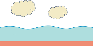
We begin by considering a thin, two-dimensional layer of an incompressible viscoelastic polymer solution in the gravitational field g (see figure 1). The solution is a binary mixture of polymeric solute and Newtonian solvent, characterized by the relaxation time $\rlap{-}{\lambda }$, viscosity ${\mu _o}$, density $\rho$, thermal conductivity $\kappa$, thermal diffusivity $\alpha$, mass diffusivity D and surface tension $\sigma$.

Figure 1. Schematic illustration of the physical system under consideration. A thin viscoelastic film (composed of a polymeric solute in a Newtonian solvent), confined between its deformable free surface $z = h(x,t)$ and a horizontal substrate in the gravitational field g, is subjected to a vertical temperature gradient. This applied temperature gradient induces a concentration gradient in the film via the Soret effect. The surface tension gradient arising from inhomogeneities in temperature and concentration at the air–liquid interface induces Marangoni convection in the liquid layer. The dashed line corresponds to the undeformed interface in the quiescent base state.

We consider the film to be of infinite horizontal extent $x \in ( - \infty ,\infty )$ with unperturbed thickness H. At the $z = 0$ plane, the film is in thermal contact with a poorly conductive rigid substrate, while a deformable free surface located at $z = h(x,t)$ separates it from the ambient gas phase. A transverse temperature gradient exists in the entire binary mixture, which is specified to be $- \vartheta$ at $z = 0$. This signifies that $\vartheta \gt 0$ $(\vartheta \lt 0)$ corresponds to the case of heating the liquid layer from the substrate (gas) side. The incorporation of the Soret effect into the analysis indicates that mass flux in the flow domain is a combination of concentration and temperature gradients (de Groot & Mazur Reference de Groot and Mazur2011). Hence, the heat ${\boldsymbol{J}_H}$ and mass ${\boldsymbol{J}_M}$ fluxes within the film are governed by

(2.1a)\begin{equation}{\boldsymbol{J}_H} ={-} \kappa {\kern 1pt} {\bf \nabla }T\end{equation}

and

(2.1b)\begin{equation}{\boldsymbol{J}_M} ={-} \rho D({\bf \nabla }c + \mathcal{S}{\kern 1pt} {\bf \nabla }T),\end{equation}

where $\mathcal{S}$ is the Soret coefficient of the mixture. For a polymeric solution, $\mathcal{S}$ can be either positive or negative depending on the solvent quality, the mole fractions of the components and the temperature of the binary mixture (Zhang & Müller-Plathe Reference Zhang and Müller-Plathe2006). A negative (positive) sign of $\mathcal{S}$ signifies the migration of polymeric solutes towards the warmer (colder) region. It follows from (2.1) that, at the conductive state, the externally applied heat flux generates a temperature difference $\Delta T = \vartheta H$, which, in turn, yields a concentration difference $\Delta c ={-} \mathcal{S}\Delta T$ across the layer.

Now, above a particular temperature gradient, the thermo- and solutocapillary effects induce Marangoni convection in this mixture. The buoyancy effect is neglected in this study considering the small thickness of the film ($H\mathrm{\ \mathbin{\lower.3ex\hbox{$\buildrel\lt \over {\smash{\scriptstyle\sim}\vphantom{_x}}$}}\ }O(1)\;\textrm{cm}$; see Pearson Reference Pearson1958). We assume the surface tension to vary linearly with temperature and solute concentration, dictated by the relationship

(2.2)\begin{equation}\sigma = {\sigma _o} - {\sigma _T}(T - {T_o}) + {\sigma _c}(c - {c_o}),\end{equation}

where ${\sigma _o}$ is the surface tension at the reference temperature ${T_o}$ and concentration ${c_o}$; and ${\sigma _T} ={-} \partial\sigma /\partial T$ and ${\sigma _c} = \partial\sigma /\partial c$ quantify the rate of change of surface tension with respect to temperature and concentration, respectively. It should be noted that for most polymeric solutions $({\sigma _T},{\sigma _c}) \gt 0$ (Doumenc et al. Reference Doumenc, Chénier, Trouette, Boeck, Delcarte, Guerrier and Rossi2013). Furthermore, except for $\sigma$, all other thermophysical properties are assumed to remain invariant with temperature in this analysis.

In the presence of a linear Soret effect, the equations governing the fields of liquid velocity $\boldsymbol{v} \equiv \{ u(x,z,t),w(x,z,t)\}$, pressure $p(x,z,t)$, temperature $T(x,z,t)$ and concentration $c(x,z,t)$ in the bulk of the film are given by

(2.3a)\begin{gather}{\bf \nabla \cdot }\boldsymbol{v} = 0,\end{gather}

(2.3b)\begin{gather}\rho \left( {\frac{{\partial \boldsymbol{v}}}{{\partial t}} + \boldsymbol{v}{\bf \cdot \nabla }\boldsymbol{v}} \right) ={-} {\bf \nabla }p + {\bf \nabla \cdot }\boldsymbol{\tau } - \rho g\boldsymbol{k},\end{gather}

(2.3c)\begin{gather}\frac{{\partial T}}{{\partial t}} + \boldsymbol{v}{\bf \cdot \nabla }T = \alpha {\nabla ^2}T,\end{gather}

(2.3d)\begin{gather}\frac{{\partial c}}{{\partial t}} + \boldsymbol{v}{\bf \cdot \nabla }c = D{\nabla ^2}c + \mathcal{S}D{\nabla ^2}T,\end{gather}

respectively, where t represents time, $\boldsymbol{\tau } = \left[ {\begin{smallmatrix}{{\boldsymbol{\tau }_{x\,x}}}&{{\boldsymbol{\tau }_{x\,z}}}\\ {{\boldsymbol{\tau }_{z\,x}}}&{{\boldsymbol{\tau }_{z\,z}}} \end{smallmatrix}} \right]$ is the deviatoric stress tensor, k is the unit vector in the z-direction and ${\bf \nabla } \equiv \{ \partial /\partial x,\partial /\partial z\}$. The above set of governing equations are accompanied by the following boundary conditions.

At the $z = 0$ plane, where the film is in thermal contact with a rigid substrate, the pertinent boundary conditions encompass the no-slip, no-penetration condition for velocity, a specified uniform normal heat flux and the mass impermeability condition, represent respectively by

(2.4a–c)\begin{equation}\boldsymbol{v} = 0,\quad \frac{{\partial T}}{{\partial z}} ={-} \vartheta ,\quad \frac{{\partial {\kern 1pt} c}}{{\partial z}} = \mathcal{S}\vartheta \quad \textrm{at}\;z = 0.\end{equation}

At the deformable free surface $z = h(x,t)$, the boundary conditions comprise the kinematic boundary condition, heat exchange with the ambient gas phase (characterized by Newton's law of cooling), mass impermeability condition and the balance of tangential and normal stress components, represented respectively by

(2.5a)\begin{gather}w = \frac{{\partial h}}{{\partial t}} + u\textrm{ }\frac{{\partial h}}{{\partial x}},\end{gather}

(2.5b)\begin{gather}- \kappa \left( {\frac{{\partial h}}{{\partial x}}\frac{{\partial T}}{{\partial x}} - \frac{{\partial T}}{{\partial z}}} \right) + q(T - {T_\infty })\sqrt {1 + {{(\partial h/\partial x)}^2}} = 0,\end{gather}

(2.5c)\begin{gather}\kappa \left( { - \frac{{\partial h}}{{\partial x}}\frac{{\partial c}}{{\partial x}} + \frac{{\partial c}}{{\partial z}}} \right) - \mathcal{S}q(T - {T_\infty })\sqrt {1 + {{(\partial h/\partial x)}^2}} = 0,\end{gather}

(2.5d)\begin{gather}\frac{1}{{\sqrt {1 + {{(\partial h/\partial x)}^2}} }}\left\{ {{\tau_{x\,z}}\left[ {1 - {{\left( {\frac{{\partial h}}{{\partial x}}} \right)}^2}} \right] + {\tau_{z{\kern 1pt} z}}\frac{{\partial h}}{{\partial x}} - {\tau_{x\,x}}\frac{{\partial h}}{{\partial x}}} \right\} = \frac{{\partial \sigma }}{{\partial x}} + \frac{{\partial \sigma }}{{\partial z}}\frac{{\partial h}}{{\partial x}},\end{gather}

(2.5e)\begin{gather}{\,-\,} p {\,+\,} \frac{1}{{1 {\,+\,} {{(\partial h/\partial x)}^2}}}\left[ {{\tau_{z{\kern 1pt} z}} {\,+\,} {\tau_{x{\kern 1pt} x}}{{\left( {\frac{{\partial h}}{{\partial x}}} \right)}^2} {\,-\,} 2\textrm{ }{\tau_{x{\kern 1pt} z}}\frac{{\partial h}}{{\partial x}}} \right] {\,=\,} \sigma \frac{{{\partial ^2}h/\partial {x^2}}}{{{{[{1 {\,+\,} {{(\partial h/\partial x)}^2}} ]}^{{3 / 2}}}}}\,\,\textrm{at}\;z = h(x,t).\end{gather}

In (2.5b,c), q denotes the rate of heat exchange between the free surface and the ambient air at temperature ${T_\infty }$. The kinematic boundary condition (2.5a) gives the interface location at time t, while the mass impermeability condition (2.5c) portrays the non-volatile behaviour of the binary mixture. The dynamics of the gas phase are decoupled here from the liquid phase by considering large differences in the physical properties between the two phases.

2.2. Constitutive model for the liquid

Viscoelastic liquids exhibit complex rheology under the simultaneous actions of viscous and elastic character. Unlike Newtonian liquids, stress exhibits here an elastic response to strain characterized by the relaxation time of the liquid. A wide variety of constitutive relationships, comprising both linear and nonlinear models, have been developed over the years to describe the rheology of viscoelastic liquids. In this analysis, we proceed with the linear Maxwell model (Maxwell Reference Maxwell1867),

(2.6)\begin{equation}\boldsymbol{\tau } + \rlap{-}{\lambda } \frac{{\partial \boldsymbol{\tau }}}{{\partial {\kern 1pt} t}} = {\mu _o}[({\bf \nabla }\boldsymbol{v}) + {({\bf \nabla }\boldsymbol{v})^\textrm{T}}],\end{equation}

which characterizes the liquid by a single relaxation time $\rlap{-}{\lambda }$ (here $\rlap{-}{\lambda }$ is interpreted as the longest relaxation time out of the spectrum of relaxation times exhibited by a viscoelastic liquid) without incorporating the rheological nonlinearity. The reasons behind adopting this particular constitutive model for this investigation are as follows. First, in the present convection phenomenon, motion is developed in a liquid film which was at rest in its equilibrium state. This indicates that the shear rates involved with the underlying process are also extremely small. A nonlinear model (viz. the upper-convected Maxwell model, wherein the ordinary time derivative of $\boldsymbol{\tau }$ in (2.6) is replaced by the ‘upper-convected’ time derivatives) is essential to describe the flow dynamics only at high shear rates. Second, since a linear stability analysis will be carried out around a quiescent base state, here any nonlinear terms in the constitutive equation will not make any contribution to the final linearized set of equations. Therefore, the stability picture obtained using a linear model will be identical to that with the inclusion of upper-convected terms. The aspects mentioned above suggest that the linearized Maxwell model is deemed sufficient to reveal the basic effect of elasticity for this analysis.

2.3. Non-dimensionalization

The boundary value problem (BVP) formulated by (2.3)–(2.5) is now non-dimensionalized by considering the unperturbed film thickness H as characteristic length scale, the thermal diffusion time ${H^2}/\alpha$ as characteristic time scale and $\vartheta H$as temperature scale.

This allows us to define the following set of dimensionless variables:

(2.7) \begin{equation}\left. \begin{array}{* {20}{c@{}}} {(\bar{x},\bar{z}) = \dfrac{{(x,z)}}{H},\quad \bar{h} = \dfrac{h}{H},\quad \bar{t} = \dfrac{t}{{{H^2}/\alpha }},\quad (\bar{u},\bar{w}) = \dfrac{{u,w}}{{(\alpha /H)}},\quad \bar{\tau } = \dfrac{\tau }{{\mu_o \alpha /{H^2}}},}\\ \bar{p} = \dfrac{p}{{\mu_o \alpha /{H^2}}},\quad \bar{T} = \dfrac{{T - {T_\infty }}}{{\vartheta H}},\quad \bar{c} = \dfrac{c}{{{\sigma_T}\vartheta H/{\sigma_c}}}. \end{array} \right\}\end{equation}

Note that, although the bulk concentration c (defined either as mass fraction or volume fraction) is a dimensionless quantity, its rescaling in the above-mentioned manner keeps this analysis coherent with the previously reported studies (Podolny et al. Reference Podolny, Oron and Nepomnyashchy2005; Shklyaev et al. Reference Shklyaev, Nepomnyashchy and Oron2009; Sarma & Mondal Reference Sarma and Mondal2018). With this choice of the non-dimensional variables, we finally obtain the governing equations and the boundary conditions (dropping the overbar sign for notational convenience) in the following dimensionless form:

(2.8a)\begin{gather}{\bf \nabla \cdot }\boldsymbol{v} = 0,\end{gather}

(2.8b)\begin{gather}P{r^{ - 1}}\left( {\frac{{\partial \boldsymbol{v}}}{{\partial t}} + \boldsymbol{v}{\bf \cdot \nabla }\boldsymbol{v}} \right) ={-} {\bf \nabla }p + {\bf \nabla \cdot }\boldsymbol{\tau } - Ga\boldsymbol{k},\end{gather}

(2.8c)\begin{gather}\frac{{\partial T}}{{\partial t}} + \boldsymbol{v}{\bf \cdot \nabla }T = {\nabla ^2}T,\end{gather}

(2.8d)\begin{gather}\frac{{\partial c}}{{\partial t}} + \boldsymbol{v}{\bf \cdot \nabla }c = Le({\nabla ^2}c + \chi {\nabla ^2}T);\end{gather}

(2.9a–c)\begin{gather}\boldsymbol{v} = 0,\quad \frac{{\partial T}}{{\partial z}} ={-} 1,\quad \frac{{\partial c}}{{\partial z}} = \chi \quad \textrm{at}\;z = 0,\end{gather}

(2.10a)\begin{gather}w = \frac{{\partial h}}{{\partial t}} + u\frac{{\partial h}}{{\partial x}},\end{gather}

(2.10b)\begin{gather}\left( {\frac{{\partial T}}{{\partial z}} - \frac{{\partial h}}{{\partial x}}\frac{{\partial T}}{{\partial x}}} \right) + BiT\sqrt {1 + {{(\partial h/\partial x)}^2}} = 0,\end{gather}

(2.10c)\begin{gather}\left( {\frac{{\partial c}}{{\partial z}} - \frac{{\partial h}}{{\partial x}}\frac{{\partial c}}{{\partial x}}} \right) - \chi BiT\sqrt {1 + {{(\partial h/\partial x)}^2}} = 0,\end{gather}

(2.10d)\begin{gather}- p + \frac{1}{{1 + {{(\partial h/\partial x)}^2}}}\left[ {{\tau_{z{\kern 1pt} z}} + {\tau_{x{\kern 1pt} x}}{{\left( {\frac{{\partial h}}{{\partial x}}} \right)}^2} - 2{\kern 1pt} {\tau_{x{\kern 1pt} z}}\frac{{\partial h}}{{\partial x}}} \right] = \varSigma \frac{{{\partial ^2}h/\partial {x^2}}}{{{{[1 + {{(\partial h/\partial x)}^2}]}^{3/2}}}},\end{gather}

(2.10e) \begin{gather} \hspace{-2pc}\dfrac{1}{{\sqrt {1 + {{(\partial h/\partial x)}^2}} }}\left\{ {{\tau_{x{\kern 1pt} z}}\left[ {1 - {{\left( {\dfrac{{\partial h}}{{\partial x}}} \right)}^2}} \right] + {\tau_{z{\kern 1pt} z}}\dfrac{{\partial h}}{{\partial x}} - {\tau_{x{\kern 1pt} x}}\dfrac{{\partial h}}{{\partial x}}} \right\}\nonumber\\ \quad\qquad = Ma\left[ { - \dfrac{{\partial T}}{{\partial x}} + \dfrac{{\partial {\kern 1pt} c}}{{\partial {\kern 1pt} x}} + {\kern 1pt} \left( { - \dfrac{{\partial T}}{{\partial z}} + \dfrac{{\partial {\kern 1pt} c}}{{\partial z}}} \right)\dfrac{{\partial h}}{{\partial {\kern 1pt} x}}} \right]\;\textrm{at}\;z = h(x,t).\end{gather}

Moreover, in non-dimensional form, the Maxwell constitutive model (2.6) reads

(2.11)\begin{equation}\boldsymbol{\tau } + De\frac{{\partial \boldsymbol{\tau }}}{{\partial t}} = [({\bf \nabla }\boldsymbol{v}) + {({\bf \nabla }\boldsymbol{v})^\textrm{T}}].\end{equation}

This problem is now characterized by the following set of dimensionless parameters: the Marangoni number Ma, the Prandtl number Pr, the Deborah number De, the (inverse) Lewis number Le, the Soret number $\chi$, the Biot number Bi, the Galileo number Ga, and the (inverse) capillary number $\varSigma$:

(2.12)\begin{equation}\left. {\begin{array}{* {20}{c@{}}} {Ma = \dfrac{{{\sigma_T}\vartheta {H^2}}}{{{\mu_o}\alpha }}\textrm{,}\quad Pr = \dfrac{{{\mu_o}}}{{\rho \alpha }},\quad De = \dfrac{{\rlap{-}{\lambda } \alpha }}{{{H^2}}},\quad Le = \dfrac{D}{\alpha },}\\ {\chi = \dfrac{{\mathcal{S}{\sigma_c}}}{{{\sigma_T}}},\quad Bi = \dfrac{{qH}}{\kappa },\quad Ga = \dfrac{{\rho g{H^3}}}{{{\mu_o}\alpha }},\quad \varSigma = \dfrac{{\sigma H}}{{{\mu_o}\alpha }}.} \end{array}} \right\}\end{equation}

The Marangoni number governs the present instability phenomenon. For the convection to set in, the thermosolutocapillary stresses must have to overcome the stabilization effects of viscous and thermal diffusion. The Marangoni number Ma gives the critical temperature difference across the film $(\vartheta H)$ at which convection appears in the film. Note that, for ${\sigma _T} \gt 0$, Ma can assume both positive and negative values depending on the direction of the applied temperature gradient $\vartheta$. A positive (negative) Ma indicates that the liquid layer is subjected to heating from below (above). However, we restrict this analysis only to positive values of Ma. The Prandtl number Pr is a material property of the liquid. Excluding the rarefied gases (which display a strong viscoelastic character with $Pr \ll 1$), for most viscoelastic liquids $Pr \gg 1$. This indicates a larger thermal diffusion time scale $({H^2}/\alpha )$ compared to the viscous diffusion time scale $(\rho {H^2}/{\mu _o})$ for such liquids. The Deborah number De is a measure of elasticity of the liquid. The value $De = 0$ indicates a Newtonian liquid ($\rlap{-}{\lambda } = 0$), while higher values of De signify enhanced elastic behaviour of the liquid. The (inverse) Lewis number Le compares the characteristic mass diffusion time scale ${H^2}/D$ to the thermal diffusion time scale ${H^2}/\alpha$. Usually Le is small for binary liquid mixtures and lies within ${10^{ - 5}} \le Le \le {10^{ - 1}}$. The Soret number $\chi$ takes into account the relative contributions of thermocapillary and solutocapillary forces to the free surface force. Note that $\chi$ can be either positive or negative based on the Soret coefficient $\mathcal{S}$ (see § 2.2). The typical value of $\chi$ varies within $- 1 \le \chi \le 1$. The Biot number Bi characterizes the heat transfer rate across the free surface. The Galileo number Ga and the (inverse) capillary number $\varSigma$ take account of the free surface deformability through the magnitude of g and $\sigma$. For a 0.1 mm thick layer of a polymeric solution with ${\mu _o} = O({10^{ - 2}})\;\textrm{Pa}\;\textrm{s}$, $\rho = O({10^3})\;\textrm{kg}\;{\textrm{m}^{ - 3}}$, $\alpha = O({10^{ - 7}})\;{\textrm{m}^2}\;{\textrm{s}^{ - 1}}$, $\sigma = O({10^{ - 2}})\;\textrm{N}\;{\textrm{m}^{ - 1}}$ and $g = O(0.1)\;\textrm{m}\;{\textrm{s}^{ - 2}}$, we obtain $Ga = 0.1$, which corresponds to the microgravity environment. It is important to note that a free surface can be treated as non-deformable in the limit $(Ga,\varSigma ) \to \infty$, which is usually the case for a liquid layer with very high surface tension in the terrestrial environment. In order to reveal the role of surface deformability on the stability characteristics of the system, we consider here two separate cases : (i) $(Ga,\varSigma ) = (0.1,{10^3})$, which represents a liquid layer with a deformable free surface in the microgravity environment, and (ii) $(Ga,\varSigma ) \to \infty$, which refers to a liquid layer with a non-deformable free surface.

4.1. Effect of elasticity and the free surface deformability

Let us first start with the monotonic instability mode. Figure 3 plots the neutral stability curves for this particular instability mode. The solid line here represents the stability threshold for a liquid layer with a deformable free surface $(Ga,\varSigma ) = (0.1,{10^3})$, while the dotted one depicts the stability margin for a non-deformable surface $(Ga,\varSigma ) \to \infty$. It can be observed that, over the entire range of disturbance wavenumber k, there exists a minimum value for the Marangoni number Ma (indicated by the marker ‘ο’; see inset of figure 3) only above which the instability first sets in in the system. We call this Ma the critical Marangoni number $(M{a_c})$ and the corresponding k and $\omega$ as the critical wavenumber $({k_c})$ and critical oscillation frequency $({\omega _c})$, respectively.

Figure 3. Neutral stability curves $Ma(k)$ for the monotonic instability mode. The solid line represents the stability threshold for a deformable free surface $(Ga,\varSigma ) = (0.1,{10^3})$, whereas the dotted line demonstrates the stability margin for a non-deformable free surface $(Ga,\varSigma ) \to \infty$. The dot (ο) mark on each neutral curve represents the critical point of the curve. The inset depicts the effect of free surface deformability on the stability threshold in the long-wave regime. Other parameters: $Bi = 0.01,\chi = 0.5$, $Le = {10^{ - 3}}$ and $Pr = 10$.

From figure 3 it is clear that, irrespective of the free surface deformability, the monotonic disturbances always emerge in the long-wave form (${k_c} \ll O(1)$). Nevertheless, the increased gravitational and surface tension forces for a non-deformable surface slightly delay the onset of these disturbances in the system ($M{a_{c,(Ga,\varSigma ) \to \infty }} \gt M{a_{c,(Ga,\varSigma ) \to (0.1,{{10}^3})}}$; see inset of figure 3). Notably, the monotonic instability threshold is not affected by the elastic behaviour of the liquid. This is due to the vanishing of any temporal components for this stationary convection (cf. (3.12)–(3.14) substituting $\lambda = 0$). The role of other non-dimensional parameters on the stability margin for this instability mode will be discussed systematically in the subsequent subsections.

We now focus our attention on the disturbances that emerge with temporal oscillations $(\omega \ne 0)$, giving rise to Hopf bifurcation. Previous investigations on the pure thermocapillary instability in a viscoelastic film (Lebon et al. Reference Lebon, Parmentier, Teller and Dauby1994; Parmentier et al. Reference Parmentier, Lebon and Regnier2000; Ramkissoon et al. Reference Ramkissoon, Ramdath, Comissiong and Rahaman2006) suggest that the oscillatory disturbances are more likely to appear in a highly viscoelastic film (highly and weakly viscoelastic liquids will be defined shortly). For the present thermosolutal convection process, we will demonstrate that, depending on the nature of the Soret coefficient (i.e. whether $\chi \gt 0$ or $\chi \lt 0$), two different oscillatory instabilities can emerge in the system. We call them the oscillatory-I and oscillatory-II modes. It is important to remark that the characteristics of the oscillatory-I mode have been extensively studied in the literature in the context of a Newtonian binary mixture (Skarda et al. Reference Skarda, Jacqmin and McCaughan1998; Podolny et al. Reference Podolny, Oron and Nepomnyashchy2005; Shklyaev et al. Reference Shklyaev, Nepomnyashchy and Oron2009; Bestehorn & Borcia Reference Bestehorn and Borcia2010). However, its behaviour for a viscoelastic binary liquid has not been investigated yet. On the other hand, to our knowledge, the oscillatory-II mode has remained entirely unexplored, even for a Newtonian binary liquid (perhaps due to limited examination over the model parameters). We will demonstrate that, for a viscoelastic binary mixture, while the oscillatory-I mode is more universal, the oscillatory-II instability can also become dominant in the system under appropriate model parameter values.

Figure 4 plots the neutral stability curves as well as the corresponding oscillation frequencies for the oscillatory-I mode. The solid and the dash-dotted lines represent here the stability margin for a deformable free surface, while their adjacent dotted lines depict the stability boundary for a non-deformable free surface.

Figure 4. (a,c) Neutral stability curves $Ma\,(k)$, and (b,d) the corresponding oscillation frequency $\omega$ for the oscillatory-I instability mode for $\chi \lt 0\textrm{ }( ={-} 0.5)$ and $\chi \gt 0\textrm{ }( = 0.5)$, respectively. For panels (a,b), the lines marked by 1 and 2 correspond to $De = 0$ and ${De = 1}$, respectively; for panels (c,d), the lines marked by 1 and 2 correspond to $De = 0.1$ and $De = 1$, respectively. In each panel, the solid and the dash-dotted lines depict the results for a deformable free surface $(Ga,\varSigma ) = (0.1,{10^3})$; the adjacent dotted line represents the results for a non-deformable free surface $(Ga\textrm{,}\varSigma ) \to \infty$. The dot (ο) mark on each neutral curve denotes the critical point (or the global minimum) of the curve. Other parameters: $Bi = 0.1$, $Le = 0.01$ and $Pr = 10$.

Figure 4(a) demonstrates that, for $\chi \lt 0$, the neutral curves consist of two branches, each characterized by a distinct local minimum. Note that, of these two minima, while one resides in the long-wave regime $({k_c} \lt O(1))$, the other lies in the short-wave regime $({k_c}\mathrm{\ \mathbin{\lower.3ex\hbox{$\buildrel\gt \over {\smash{\scriptstyle\sim}\vphantom{_x}}$}}\ }O(1))$. Accordingly, we call these branches the long-wave and short-wave branch, respectively. It can be clearly seen that, for the long-wave branch, $M{a_c}$ is a strong function of the deformability of the free surface. Similar to the monotonic mode, a reduced free surface deformability enhances the stability of the system against the long-wave oscillatory-I disturbances as well. However, the onset of these disturbances essentially remains unaffected by the elastic behaviour of the liquid (see figure 4a; the long-wave branch for $De = 0$ and 1 merge into a single curve). On the other hand, $M{a_c}$ for the short-wave branch is not influenced by the deformability of the free surface, but is governed by the elasticity of the mixture. An increased elasticity of the liquid substantially promotes here the onset of instability in the system. This suggests that, depending on the free surface deformability and the elasticity level of the liquid, either of the long-wave or short-wave branches can hold the position of global minimum (see the marker ‘ο’ on each neutral curve in figure 4a). In other words, the oscillatory-I disturbances can emerge in both the long-wave and short-wave form for $\chi \lt 0$.

Figure 4(c) shows that, for $\chi \gt 0$, the long-wave branch disappears, leaving only the short-wave branch. In particular, in this regime of $\chi$, the oscillatory-I disturbances are found only for $De \gt 0$. This indicates that the emergence of short-wave oscillatory-I instability for $\chi \gt 0$ is a sole manifestation of the elastic behaviour of the liquid. Similarly to the case $\chi \lt 0$, the stability threshold remains unaltered by the deformability of the free surface but diminishes drastically with the increasing elasticity of the mixture.

The oscillation frequency $\omega$ of the neutral perturbations corresponding to each neutral curve of figure 4(a,c) is plotted in figure 4(b,d). The deformability of the free surface controls $\omega$ only in the long-wave regime, whereas $\omega$ is primarily modulated by the elasticity of the liquid in the short-wave regime. It should be further noted that, although the $\omega \,(k)$ variation is smooth in the long-wave regime, discontinuity appears in the short-wave regime (in particular at higher values of De). In the neighbourhood of such points of discontinuity, a sudden change in the gradient of Ma(k) neutral curve occurs, as can be observed from figure 4(a,c). Similar features of the neutral curves have been reported previously by Dauby et al. (Reference Dauby, Parmentier, Lebon and Grmela1993) and Parmentier et al. (Reference Parmentier, Lebon and Regnier2000) in the context of pure thermocapillary-driven convection in a viscoelastic film.

It is now clear that, for $\chi \lt 0$, the oscillatory-I disturbances can develop in both Newtonian and viscoelastic binary mixtures. However, the elasticity of the liquid significantly influences the onset of this particular instability mode in the system. To illustrate this elasticity-based transition of the stability picture, we plot in figure 5 the critical Marangoni number $M{a_c}$, the corresponding wavenumber ${k_c}$, and oscillation frequency ${\omega _c}$ as functions of Deborah number De for both the cases of deformable (solid line) and non-deformable (dotted line) free surface. Note that $M{a_c}$ refers here to the global minimum of the oscillatory-I neutral curve. Two regimes are clearly distinguishable from the variations depicted by figure 5: a weakly elastic regime (for $De\mathrm{\ \mathbin{\lower.3ex\hbox{$\buildrel\lt \over {\smash{\scriptstyle\sim}\vphantom{_x}}$}}\ }0.1$) wherein the stability behaviour resembles that of a Newtonian binary liquid (at least for bifurcation around the conductive base state), and a strong elastic regime (for $De \gt 0.1$) where the elasticity of the liquid governs the stability threshold and the critical parameters $({k_c},{\omega _c})$. The transition between these two regimes is marked by sharp discontinuities in ${k_c}$ and ${\omega _c}$ (see the arrow marks in figure 5b,c).

Figure 5. Variation of the (a) critical Marangoni number $M{a_c}$, and the corresponding critical (b) wavenumber ${k_c}$ and (c) oscillation frequency ${\omega _c}$ with Deborah number De for the oscillatory-I instability mode for $\chi \lt 0$. The solid line depicts the variation for a deformable free surface $(Ga,\varSigma ) = (0.1,{10^3})$; and the dotted line is that for a non-deformable surface $(Ga,\varSigma ) \to \infty$. The arrow marks in panels (b,c) illustrate a switchover in the instability behaviour with the increasing elasticity of the liquid. Other parameters: $Bi = 0.1$, $Le = 0.01$ and $\chi ={-} 0.5$.

A key observation from figure 5 is that, in the weakly elastic regime, while the critical parameters ($M{a_c},{k_c},{\omega _c}$) are governed by the deformability of the free surface rather than the elasticity of the liquid, the opposite is true for the highly elastic regime. Figure 5(a) shows that the reducing deformability of the free surface dampens the onset of oscillatory-I instability for $De\mathrm{\ \mathbin{\lower.3ex\hbox{$\buildrel\lt \over {\smash{\scriptstyle\sim}\vphantom{_x}}$}}\ }0.1$. The resulting disturbances emerge in the long-wave form (${k_c} \approx 0.1$) for a deformable free surface and the short-wave form (${k_c} \approx 1$) in case of a non-deformable free surface (see figure 5b). On the other hand, for a highly viscoelastic mixture ($De \gt 0.1$), irrespective of the free surface deformability, the disturbances always set in in the short-wavelength form. An inverse variation of the parameters ($M{a_c},{k_c},{\omega _c}$) with De in this regime suggests that, for the enhanced elasticity of the binary mixture, the conductive state is more likely to bifurcate to the short-wave oscillatory-I mode with a more easily detectable convective pattern.

Another interesting feature presented by figure 5 is that, for $De \approx 0.1$ (i.e. the boundary separating the weakly and highly elastic regimes for a liquid layer with a deformable free surface), $M{a_c}$ for the onset of long-wave and short-wave oscillatory-I perturbations coincide. Therefore, a competition between the respective instability modes can take place in the system for $(De,Ga,\varSigma ) \approx (0.1,0.1,{10^3})$.

4.2. The role of thermocapillary and solutocapillary effects

In this subsection, we investigate the contributions of thermocapillary and solutocapillary forces on the development of instabilities in the system. This is done by plotting the neutral stability curves for monotonic and oscillatory modes at different values of $\chi$. Recall that $\chi = 0$ refers in this analysis to the case of purely thermocapillary-driven convection. Figure 6(a) shows that the domain of stability reduces substantially as $\chi$ increases from zero. This suggests that both thermocapillary and solutocapillary forces play a destabilizing role in the emergence of monotonic instability for $\chi \gt 0$. However, it is important to note that ${k_c}$ for this instability mode is not decided by the solutal effects (at least for a deformable surface; the case of a non-deformable surface will be discussed in figure 7). Although not shown here graphically, this particular instability mode can appear even for $\chi \lt 0$, within a narrow interval of $\chi$. This range will be identified in § 6, performing a long-wave asymptotic analysis of the problem.

Figure 6. Neutral stability curves $Ma(k)$ for the monotonic and oscillatory-I modes in the (a,c) positive and (b) negative Soret number $\chi$ domains. The long-wave branch for the oscillatory-I mode emerges only when $\chi \lt 0$. The dot (ο) mark on each neutral curve represents the critical point of the curve. Other parameters: $Bi = 0.01$, $De = 1$, $Le = {10^{ - 3}}$ and $(Ga,\varSigma ) = (0.1,{10^3})$.

Figure 7. Variation of the (a) critical Marangoni number $M{a_c}$, and the corresponding (b) critical wavenumber ${k_c}$ with $\chi$. In each panel, the solid, dash-dotted and dashed lines represent the variations for a deformable free surface $(Ga,\varSigma ) = (0.1,{10^3})$. The dotted lines adjacent to each instability mode represent the variations for a non-deformable free surface $(Ga,\varSigma ) \to \infty$. Other parameters: $Bi = 0.01$ and $Le = {10^{ - 3}}$.

Figure 6(b) demonstrates that, for the long-wave branch of oscillatory-I mode, solutocapillarity acts as stabilizing, while thermocapillarity turns into the destabilizing mechanism. Such opposite contributions of the driving forces give rise to the long-wave oscillatory-I perturbations in the system. On the other hand, thermocapillarity, coupled with the elasticity of the liquid, primarily give rise to the short-wave disturbances. Solutocapillarity provides here only a small correction to the stability margin. Interestingly, for this short-wave branch, an increasing $|\chi |$ in the range $\chi \lt 0$ weakly destabilizes the system, whereas an increment in $\chi$ for $\chi \gt 0$ leads to a mild stabilization of the system (see insets in figure 6b,c).

Figure 7 plots the variations of critical Marangoni number $M{a_c}$ and the corresponding wavenumber ${k_c}$ with $\chi$ for the cases of both a deformable and a non-deformable free surface. Clearly, an increasing $\chi \;( \gt 0)$ leads to a strong destabilization of the system with respect to the monotonic disturbances (see figure 7a). It should be noted that, for this instability mode, although the deformability of the free surface only weakly influences the stability threshold (see figure 3; this is not even perceptible in the scale of figure 7a), nevertheless, it plays an important role in determining the size of the convection cells. In figure 7(b) one can see that ${k_{c,(Ga,\varSigma ) \to \infty }} \gt {k_{c,(Ga,\varSigma ) = {\kern 1pt} (0.1,{{10}^3})}}$, implying that a highly deformable free surface allows the formation of much larger sized stationary convective patterns compared to its non-deformable counterpart.

For the oscillatory-I mode, figure 7(a) shows that an increasing $|\chi |$ augments the stability region for a Newtonian binary liquid film having a deformable free surface. However, in the case of a non-deformable free surface (or for a highly viscoelastic mixture irrespective of the free surface deformability), the stability thresholds are found to remain nearly independent of $\chi$. In this regard, it is important to observe in figure 7(b) that, for a Newtonian binary mixture with a deformable surface, ${k_c}$ lies in the long-wave regime, whereas, for a non-deformable surface (or for a highly viscoelastic mixture), ${k_c}$ resides in the short-wave regime. The fact that the solutocapillary effect is dominant only in the long-wave regime (see figure 6) thus explains the variations in figure 7(a).

Before concluding this subsection, an additional remark about figure 7(a) is necessary. Note that, at the intersection point between the neutral curves for monotonic and oscillatory-I modes, $M{a_{c,mon}} = M{a_{c,osc. \text{-} I}}$. Therefore, a competition between the respective instability modes can occur for $\chi$ values corresponding to this point. Now, for $De \gt 0$, since the oscillatory-I disturbances can appear for any $\chi \in {\mathbb R}$, and as their onset gets triggered by the increasing elasticity of the liquid, the neutral curve for the monotonic mode presented in figure 7(a) is essentially the locus of codimension-two bifurcation points. Towards the left of this curve, the conductive state bifurcates into the oscillatory-I mode, while a steady bifurcation (i.e. monotonic instability) takes place on its right.

4.3. The role of thermal and solutal diffusivities

Let us now discuss the influence of thermal and solutal diffusivities on the onset of instability in the system. Here, we will demonstrate that, based on the diffusivity ratio $Le\;( = D/\alpha )$, a different kind of oscillatory instability (i.e. oscillatory-II) can emerge in the liquid layer. Before that, we first investigate the role played by Le on the emergence of oscillatory-I disturbances.

Figure 8(a) shows that an increased solute diffusivity corresponding to higher values of Le enhances the stability of the system against the long-wave oscillatory-I disturbances. This is due to the stabilizing role of solutocapillarity (see figure 6b) in producing this instability mode. Similarly, a destabilizing (stabilizing) solutocapillary force for $\chi \lt 0\textrm{ }(\chi \gt 0)$ in the short-wave regime leads to a reduction (enhancement) in the stability threshold for higher solute diffusivity (compare figure 8a,b with figure 6b,c).

Figure 8. Effect of Lewis number Le on the monotonic and oscillatory instability threshold for (a,c) $\chi \lt 0\textrm{ }( ={-} 0.5)$ and (b) $\chi \gt 0{\kern 1pt} \textrm{ }( = 0.5)$. The dot (ο) mark on each neutral curve represents the critical point of the curve. Panel (c) shows that, for a deformable free surface at higher value of Le, a different type of long-wave oscillatory instability (oscillatory-II) can emerge in the fluid layer. Other parameters: $Bi = 0.01$, $De = 1$ and $(Ga,\varSigma ) = (0.1,{10^3})$.

Figure 8(c) shows that, for a sufficiently large Le ($\mathrm{\ \mathbin{\lower.3ex\hbox{$\buildrel\gt \over {\smash{\scriptstyle\sim}\vphantom{_x}}$}}\ }O({10^{ - 2}})$), the oscillatory-II disturbances can emerge in systems with a deformable free surface. Note that, at higher k values, the neutral curve for this particular instability mode (the dotted line) merges with the neutral curve for the monotonic mode (the solid line). This limits the appearance of oscillatory-II disturbances only in the long-wave form.

The other features of this instability mode are also quite different from those of the oscillatory-I mode. First, while the oscillatory-I instability can emerge in the system for the entire permissible range of model parameters, the oscillatory-II instability appears only in the case of a deformable free surface, for $\chi \gt 0$ and $Le\mathrm{\ \mathbin{\lower.3ex\hbox{$\buildrel\gt \over {\smash{\scriptstyle\sim}\vphantom{_x}}$}}\ }O({10^{ - 2}})$. Although not shown here graphically, such disturbances get damped with the reducing deformability of the free surface and eventually disappear in a non-deformable free surface. Second, the oscillation frequency of the oscillatory-II mode is several orders of magnitude smaller than that of the oscillatory-I mode (see figure 9). This suggests that the oscillatory-II perturbations develop with a significantly large oscillation period compared to the oscillatory-I disturbances.

Figure 9. Comparison of the oscillation frequency of neutral perturbations for the oscillatory-II mode with oscillatory-I mode (shown in the inset). Parameters: $\chi = 0.5$, $Bi = 0.01$, $De = 1$, $Le = 0.1$ and $(Ga,\varSigma ) = (0.1,{10^3})$.

Now, in order to understand the physical mechanism behind the origination of the oscillatory-II disturbances and to elucidate the role of liquid elasticity on their onset, we plot in figure 10 the variation of $M{a_c}(\chi )$ with De for this instability mode. The disappearance of these disturbances for purely thermocapillary-driven convection ($M{a_c} \to \infty$ as $\chi \to 0$) and the reduction of $M{a_c}$ with $\chi$ suggest that the competition between stabilizing thermocapillary and destabilizing solutocapillary forces gives rise to the oscillatory-II mode. A shorter mass diffusion time scale $({H^2}/D)$ is here essential to overcome the stabilizing action of thermocapillarity by the destabilizing solutocapillary force. This explains the reason behind the emergence of oscillatory-II instability only for higher values of Le $( = ({H^2}/\alpha )/({H^2}/D)\mathrm{\ \mathbin{\lower.3ex\hbox{$\buildrel\gt \over {\smash{\scriptstyle\sim}\vphantom{_x}}$}}\ }O({10^{ - 2}}))$. Another key observation from figure 10 is that the $M{a_c}(\chi )$ neutral curves for different values of $De$ (= 0 and 1) collapse onto a single curve. This implies that the stability threshold for the oscillatory-II mode is not affected by the elastic behaviour of the binary mixture.

Figure 10. Variation of the critical Marangoni number $M{a_c}$ with $\chi$ for the oscillatory-II mode at $Bi = 0.01$, $Le = 0.1$ and $(Ga,\varSigma ) = (0.1,{10^3})$. Note that no oscillatory-II instability emerges for $\chi \le 0$.

4.4. The role of heat transfer rate at the free surface

Lastly, we discuss the role of the Biot number on the stability threshold of the system. In figure 11, the neutral stability curves for each instability mode are plotted for two different values of Bi ($= {10^{ - 3}}$ and 0.1). It turns out that, at higher values of Bi, the enhanced heat transfer rate from the free surface increases the stability of the system against the long-wave disturbances (see figure 11(a,c,d) at small k). However, the influence of Bi is less significant in the short-wave regime, as reflected by the saturation of curves in this regime (see figure 11(a–c) at large k). The magnitude of Bi, therefore, bears significant importance in the emergence of long-wave instability in the liquid layer.

Figure 11. Effect of Biot number Bi on the monotonic and oscillatory instability threshold for (a) $\chi \lt 0\textrm{ }( ={-} 0.5)$, and (b,c,d) $\chi \gt 0\textrm{ }( = 0.5)$ for a film with deformable free surface $(Ga,\varSigma ) = (0.1,{10^3})$. Other parameters: $De = 1$ and $Le = 0.01$.

6.1. Monotonic mode

Let us start with the case of monotonic instability. Substitution of ${\lambda _o} = 0$ into (6.13) yields the explicit expression for the neutral stability curve of this instability mode:

(6.14)\begin{equation}M{a_{mon.}} = \frac{{48Le\mathcal{Q}(\mathcal{B} + {q^2})}}{{\mathcal{B}\chi {\kern 1pt} \mathcal{Q}{\kern 1pt} + {\kern 1pt} [\mathcal{Q}\chi + Le(72 + \mathcal{Q})(1 + \chi )]{q^2}}}.\end{equation}

Returning to the unscaled parameters k, Bi and $\varSigma$, we get

(6.15)\begin{equation}M{a_{mon.}} = \frac{{48Le(Ga + \varSigma {k^2})(Bi + {k^2})}}{{Bi\chi (Ga + \varSigma {\kern 1pt} {k^2}) + {\kern 1pt} [{\chi (Ga + \varSigma {k^2}) + Le(1 + \chi )(72 + Ga + \varSigma {k^2})} ]{k^2}}}.\end{equation}

Equation (6.15) depicts the stability boundary for a system with deformable free surface. For a non-deformable surface (i.e. in the limit $(Ga + \varSigma {k^2}) \to \infty$), the stability margin (6.15) becomes

(6.16)\begin{equation}M{a_{mon.}} = \frac{{48Le(Bi + {k^2})}}{{Bi\chi + (Le + \chi + Le{\kern 1pt} \chi ){k^2}}}.\end{equation}

The minimization of (6.15) for Ma now yields the following expression for critical wavenumber ${k_c}$:

(6.17)\begin{equation}{k_c} = \sqrt {\frac{{BiGa\varSigma + \sqrt {72BiGa\varSigma (72 + Ga - Bi\varSigma )} }}{{\varSigma (72 - Bi\varSigma )}}} \quad \textrm{for}\;\chi \ne - 1.\end{equation}

Interestingly, (6.17) also indicates the domain of validity of this approximate model. Note that, for $Bi\varSigma = 72$, one has ${k_c} \to \infty$, violating the lubrication approximation, $k \ll 1$. Therefore, the proposed model holds good only for $Bi{\kern 1pt} \varSigma \lt 72$. This event is graphically demonstrated in figure 14. One can readily see that the critical parameters $(M{a_c},{k_c})$ predicted by the long-wave theory agree with the numerical results only for $Bi{\kern 1pt} \varSigma = 10\;( \lt 72)$ (i.e. for a deformable free surface, see figure 14a).

Figure 14. Comparison of results obtained from the approximate model (solid and dash-dotted lines) with the numerical results (dotted lines) for the monotonic instability mode via the neutral stability curve (a) deformable surface $(Ga,\varSigma ) = (0.1,\,{10^3})$, and (b) non-deformable surface $(Ga,\varSigma ) \to \infty$. The dot (ο) mark on each neutral curve represents the critical point of the curve. Other parameters: $Bi = 0.01$ and $Le = 0.1$.

Equations (6.15) and (6.16) indicate that, at $k \to \infty$, irrespective of the deformability of the free surface, Ma attains the limiting value

(6.18)\begin{equation}M{a_{mon.,k \to \infty }} = \frac{{48Le}}{{Le + \chi + Le\chi }}.\end{equation}

It should be noted that, for $Bi{\kern 1pt} \varSigma \ge 72$, $Ma \to M{a_c}$ in (6.18). However, this $M{a_c}$ has lost the quantitative agreement with the numerical results owing to the violation of the long-wave approximation (compare panels figure 14a,b).

From (6.15) and (6.16) it further follows that, for $k \in [0,\infty )$, irrespective of the deformability of the free surface, Ma remains positive for $\chi \gt 0$ and becomes negative when $\chi \lt - Le/(1 + Le)$. Hence, there must be a discontinuity in the neutral curves in the domain $0 \gt \chi \gt - Le/(1 + Le)$, suggesting the emergence of instability for heating from the top as well as from below. For the case of a deformable free surface, this point of discontinuity (${k_d}$) is given by the real and positive root of

(6.19)\begin{equation}{\gamma _0}{\kern 1pt} k_d^4 + {\gamma _1}k_d^2 + {\gamma _2} = 0;\end{equation}

the coefficients ${\gamma _j}$ (j = 0–2) are presented in appendix B.

On the other hand, for a non-deformable surface, the point of discontinuity ($k_d^{nd}$) lies at

(6.20)\begin{equation}k_d^{nd} = \sqrt { - \frac{{Bi\chi }}{{Le + \chi + Le\chi }}} .\end{equation}

Thus, for $\chi \in ({0, - Le/(1 + Le)} )$, the monotonic instability sets in for heating the liquid layer from below with $k \gt {k_d}$ (or $k_d^{nd}$ for a non-deformable surface) and vice versa. For the parameter values $(Le,\chi ) = (0.1, - 0.05)$ this situation is graphically illustrated in figure 14. Here, ${k_d} = 2.8 \times {10^{ - 3}}$ and $k_d^{nd} = 0.105$ (see figure 14a,b). A comprehensive study of the stability characteristics of the branch pertaining to the negative values of Ma is beyond the scope of this paper.

Finally, a few previously reported results in the literature can be derived from the expressions (6.15) and (6.16). Since the monotonic instability threshold remains unaffected by the elastic behaviour of the liquid, therefore, in the limit $\chi = 0$, (6.15) yields the results for purely thermocapillary-driven convection in a Newtonian liquid layer (Shklyaev, Alabuzhev & Khenner Reference Shklyaev, Alabuzhev and Khenner2012). For such a film, (6.16) yields the well-known asymptotic value $M{a_{mon.}} = 48$ in the limit $(Ga,\varSigma ) \to \infty$, for either $Bi = 0$ or $k \to \infty$ (Pearson Reference Pearson1958).

6.2. Oscillatory mode

The stability threshold for this instability mode is obtained by substituting ${\lambda _o} = \textrm{i}\omega$ in (6.13). This yields

(6.21)\begin{equation}M{a_{ {\pm} {\kern 1pt} osc.}} = \frac{{({\mathcal{N}_0} - \omega _ \pm ^2{\mathcal{N}_2})({\mathcal{D}_0} - \omega _ \pm ^2{\mathcal{D}_2}) + \omega _ \pm ^2({\mathcal{N}_1} - \omega _ \pm ^2{\mathcal{N}_3})({\mathcal{D}_1} - \omega _ \pm ^2{\mathcal{D}_3})}}{{{{({\mathcal{D}_0} - \omega _ \pm ^2{\mathcal{D}_2})}^2} + \omega _ \pm ^2{{({\mathcal{D}_1} - \omega _ \pm ^2{\mathcal{D}_3})}^2}}},\end{equation}

where ${\omega _ \pm } = ({\omega _ + },{\omega _ - })$ are the oscillation frequencies for $M{a_{ {\pm} osc.}} = (M{a_{ + osc.}},M{a_{ - osc.}})$, respectively, and are given by

(6.22)\begin{align}\omega _ \pm ^2 & = \dfrac{1}{{2({{\mathcal{N}_3}{\mathcal{D}_2} - {\mathcal{N}_2}{\mathcal{D}_3}} )}}[({{\mathcal{N}_1}{\mathcal{D}_2} + {\mathcal{N}_3}{\mathcal{D}_0} - {\mathcal{N}_2}{\mathcal{D}_1} - {\mathcal{N}_0}{\mathcal{D}_3}} )\notag\\ & \quad \pm \sqrt {{{({{\mathcal{N}_2}{\mathcal{D}_1} + {\mathcal{N}_0}{\mathcal{D}_3} - {\mathcal{N}_1}{\mathcal{D}_2} - {\mathcal{N}_3}{\mathcal{D}_0}} )}^2} - 4({{\mathcal{N}_3}{\mathcal{D}_2} - {\mathcal{N}_2}{\mathcal{D}_3}} )({{\mathcal{N}_1}{\mathcal{D}_0} - {\mathcal{N}_2}{\mathcal{D}_3}} )} ]. \end{align}

Note that $\omega _ + ^2\;(\omega _ - ^2)$ refers to the oscillation frequency obtained from adding (subtracting) the square root terms in the numerator of (6.22). For a given set of model parameters $(\mathcal{B},Ca,\mathcal{D}e,Ga,Le,\chi )$, the presence of two different oscillation frequencies (i.e. ${\omega _ + }$ and ${\omega _ - }$) suggests the possible emergence of two different oscillatory instabilities in the system (namely, oscillatory-I and oscillatory-II, as discussed in § 4). Confirming the numerical results, one of the oscillation frequencies vanishes for a non-deformable surface (must be the one related with the oscillatory-II mode), for which the expressions of the neutral curve and oscillation frequency are given by

(6.23)\begin{equation}M{a_{osc.}} = \frac{{48(Bi + {k^2} + Le{k^2})}}{{[(1 + De{\kern 1pt} Le{k^2}) + \chi (1 + BiDe + De{k^2} + De{\kern 1pt} Le{k^2})]{k^2}}}\end{equation}

and

(6.24)\begin{equation}{\omega ^2} = \frac{{{\mathcal{L}_0}{k^6} + {\mathcal{L}_1}{k^4} + {\mathcal{L}_2}{k^2} + {\mathcal{L}_3}}}{{{\mathcal{L}_4}{\kern 1pt} {k^2} + {\mathcal{L}_5}}},\end{equation}

respectively. The coefficients ${\mathcal{L}_j}$ (j = 0–5) are defined in appendix C. It is worth noting that, in the limit $De = 0$, (6.23) matches with the results for a Newtonian liquid (Podolny et al. Reference Podolny, Oron and Nepomnyashchy2005).

Given the convoluted form of the neutral curves (6.21) and (6.23), any further analytical progress in estimating their validity bound now becomes a rather intricate task. Thus, we verify the accuracy of this analysis by comparing the results with numerical computations for a wide range of the parameters $(De,Le,\chi )$ within the limit $Bi\varSigma \lt 72$. For the long-wave branch of oscillatory-I mode, figure 15(a) shows that the results obtained from the approximate model agree with the numerical results in an excellent manner for both the Newtonian $(De = 0)$ and highly viscoelastic $(De = 10)$ binary mixtures. Here, the oscillation frequency is given by ${\omega _ - }$. However, this agreement is found to be poor for the short-wave branch, due to the violation of the lubrication approximation (see figure 15b). Nevertheless, the scaling adopted for De (see 6.2b) helps in achieving a qualitative agreement at higher values of De. The oscillation frequency for this branch is given by ${\omega _ + }$.

Figure 15. Comparison between results of the numerical computation (dotted lines) and the approximate model (solid and dash-dotted lines) for the oscillatory-I mode via neutral stability curve: (a) long-wave branch at $Le = 0.1$, $\chi ={-} 0.5$; and (b) short-wave branch at $Le = {10^{ - 3}}$, $\chi = 0.5$. Other parameters: $Bi = 0.01$ and $(Ga,\varSigma ) = (0.1,{10^3})$.

Finally, this approximate model also predicts the emergence of oscillatory-II instability in the system. The oscillation frequency for this mode is given by ${\omega _ - }$. Figure 16 shows that the developed model is capable of depicting the stability threshold in a fairly accurate manner for this instability mode as well.

Figure 16. Comparison of results obtained from the approximate model (solid and dash-dotted lines) with the numerical results (dotted lines) for the oscillatory-II mode via the neutral stability curve at $Bi = 0.01$, $De = 1$, $Le = 0.1$ and $(Ga,\varSigma ) = (0.1,{10^3})$.