


1 Introduction
Unsteady flow in porous media has been the subject of active research over at least the past 60 years. One of the main interests has been the propagation of acoustic waves in porous structures, which has applications in seismic waves, enhanced oil recovery, ocean bottom interactions and coastal waves, superfluid flow in porous media, among many others, in addition to the fundamental nature of deriving appropriate physical models. This was initiated by the pioneering works of Biot (Reference Biot1956a ,Reference Biot b ) to analyse effects such as wave speed, attenuation, viscous dissipation and anisotropy. An overview of the literature on the subject may lead to the classification of studies into three main groups: studies about elastic media without any fluid external forcing; studies of time-dependent flow in rigid porous media; and studies of fluid flow through elastic media. In the present work, the interest is focused upon incompressible and unsteady single-phase flow through rigid homogeneous periodic porous media. Existing reported works may be conveniently summarized by distinguishing those carried out in the time domain from those developed in the frequency domain. In the following paragraphs, a non-exhaustive literature review of both branches is presented.
The description of unsteady incompressible one-phase flow in porous media has been widely reliant on extensions to the steady version of Darcy’s law, or, when inertia is taken into account, the Darcy–Forchheimer corrected form. To the best of our knowledge, one of the earliest extensions to account for unsteady effects was put forward by Polubarinova-Kochina (Reference Polubarinova-Kochina1962). In this work, an acceleration term on the filtration velocity was kept in the macroscopic momentum equation as obtained from a direct analogy with the Stokes (or Navier–Stokes) equation in which the point velocity is replaced by the average velocity and the external force by the average friction on the solid surface of the porous matrix, i.e. the Darcy term. Despite its lack of rigorous formal derivation, this type of approach has been considered as a valid one and became classical over the past half-century (Rajagopal Reference Rajagopal2007; Bories et al. Reference Bories, Mojtabi, Prat and Quintard2008; Nield & Bejan Reference Nield and Bejan2013). This model will be referred to as the ‘heuristic model’. It has been widely used, for instance, in numerical simulations (Dogru, Alexander & Panton Reference Dogru, Alexander and Panton1978), for stability analysis of fluid flow between an impermeable plate and a porous wall (Hill & Straughan Reference Hill and Straughan2008, Reference Hill and Straughan2009) or for turbulence in a similar configuration (Breugem, Boersma & Uittenbogaard Reference Breugem, Boersma and Uittenbogaard2006) or in a confined porous medium (Jin & Kuznetsov Reference Jin and Kuznetsov2017), as well as for three-dimensional stability analysis of flow between two parallel porous walls (Tilton & Cortelezzi Reference Tilton and Cortelezzi2008), for the analysis of forced or natural convection in porous media (Kuznetsov & Nield Reference Kuznetsov and Nield2006), and for the transition to chaos in natural convection (Vadasz Reference Vadasz1999), among many other applications.
A few formal analyses have been dedicated to tentatively derive the heuristic model and some of them may have been inspired by the development of the steady macroscopic model of one-phase flow in porous media including inertia by Whitaker (Reference Whitaker1996). In fact, in this reference, the acceleration term was kept in a large part of the development although it was clearly stated, at the final stage, that the steady ancillary closure problem used to derive the closed average model was only compatible with a steady version of this model (see § 2.8 in Whitaker (Reference Whitaker1996)). However, the unsteady version of this model was used by Tilton & Cortelezzi (Reference Tilton and Cortelezzi2008) with a reference to Whitaker (Reference Whitaker1996). Two other works (Teng & Zhao Reference Teng and Zhao2000; Breugem et al. Reference Breugem, Boersma and Uittenbogaard2006) proposed a development yielding the unsteady form of the macroscopic model developed by Whitaker (Reference Whitaker1996, equation (2.26)) that, indeed, corresponds to the heuristic model. However, in these works, the closure procedure is not considered and the time-scale constraint is not addressed. Nevertheless, in a recent paper, Zhu et al. (Reference Zhu, Waluga, Wohlmuth and Manhart2014) further considered this version of the unsteady model and showed, from comparison with direct numerical simulation (DNS), that it was inappropriate. For the sake of keeping the same form of the unsteady model, the acceleration term was modified by conveniently introducing a time constant obtained by averaging the energy equation, an idea that was employed by Laushey & Popat (Reference Laushey, Popat and Tison1968) to interpret results obtained on model unconfined aquifers. Comparisons with DNS results showed agreement. However, this time constant requires knowledge of the pore-scale flow field featuring a non-closed overall model that cannot be used as a predictive one even under creeping flow conditions.
The approach making use of the heuristic model has also been very popular in wave dampening models in coastal engineering (Hall, Smith & Turcke Reference Hall, Smith and Turcke1995; Corvaro et al. Reference Corvaro, Mancinelli, Brocchini, Seta and Lorenzoni2010). In this field, however, the lack of accuracy of the approach, compared to experimental data, led numerous authors to modify the heuristic model by affecting a pre-multiplying factor, usually called ‘inertial coefficient’, to the accumulation term. Without any formal derivation, this was justified by an analogous concept of an added virtual mass force used for modelling flow around an isolated obstacle. This concept was first introduced by Sollitt & Cross (Reference Sollitt and Cross1972) and many different forms of the inertial coefficient have been proposed since then (see the short review in Burcharth & Andersen (Reference Burcharth and Andersen1995)). A formal derivation of this modified version of the heuristic model was attempted (Abderahmane et al. Reference Abderahmane, Khalifa, Wahyudi and Thomas2002) but the development suffers again, at the final stage, from a formal identification of the macroscopic model to be obtained with the microscopic model. The misleading use of the heuristic model was pointed out by Auriault (Reference Auriault1999), indicating that the macroscopic momentum equation should contain a memory effect expressed by a convolution product between the filtration velocity and a memory function. The proof of this form was anticipated by the same author (Auriault Reference Auriault1980), and almost simultaneously by Lions (Reference Lions1981). It was later reconsidered by Allaire (Reference Allaire1992), Mikelić (Reference Mikelić1994) and, more recently, in Mei & Vernescu (Reference Mei and Vernescu2010) (the term ‘permeability’ attributed to the memory function in the latter references is inadequate, as it is dimensionally incorrect). However, as will be commented upon in the following sections, the reported developments need to be completed, either by taking into account the initial condition or by explicitly providing the closure problems yielding the effective coefficients, in particular in the case where inertia is significant. Upscaling the Navier–Stokes (or Euler) equations was also addressed using the homogenization technique (Sanchez-Palencia Reference Sanchez-Palencia1980; Masmoudi Reference Masmoudi1998, Reference Masmoudi2002; Lions & Masmoudi Reference Lions and Masmoudi2005). However, as will be further commented upon in § 3.2, no complete unsteady macroscopic model was reported with this technique. Some other derivations were reported in the literature, mainly developed in the Fourier domain.
Regarding the literature about unsteady flow modelling in porous media in the frequency domain, it is worth mentioning that one serious drawback of Biot’s early theory lies in the lack of providing numerical predictions of the effective-medium coefficients involved in the macroscale model. This issue was addressed by Auriault, Borne & Chambon (Reference Auriault, Borne and Chambon1985), who used the homogenization technique to derive a Darcy-law-type model to describe unsteady creeping flow in rigid and deformable porous media, assuming the fluid to be at rest in the porous matrix as the initial condition. Predictions of the model were validated with experimental results. This study is a continuation of previous works by Lévy (Reference Lévy1979) and Auriault (Reference Auriault1980), where the homogenization method was used to study flow through elastic porous media. In the work by Lévy, the resulting expression is also a Darcy-law-type model in the frequency domain, while the work by Auriault is an extension to include inertial effects and multiphase flow. This upscaling approach was also used by Sheng & Zhou (Reference Sheng and Zhou1988) (see also Zhou & Sheng Reference Zhou and Sheng1989) to predict the dynamic permeability as a function of frequency for a variety of microstructures in the creeping flow regime. These authors proposed to scale the predicted dynamic permeability,
 $\unicode[STIX]{x1D705}(\unicode[STIX]{x1D714})$
, by its static value,
$\unicode[STIX]{x1D705}(\unicode[STIX]{x1D714})$
, by its static value,
 $\unicode[STIX]{x1D705}_{0}$
, in order to produce a universal curve independent of the microstructure when plotted against a scaled frequency (
$\unicode[STIX]{x1D705}_{0}$
, in order to produce a universal curve independent of the microstructure when plotted against a scaled frequency (
 $\unicode[STIX]{x1D714}_{c}$
) that is particular to the microscale geometry and flow properties. In this way, these authors proposed the empirical relationship
$\unicode[STIX]{x1D714}_{c}$
) that is particular to the microscale geometry and flow properties. In this way, these authors proposed the empirical relationship
 $$\begin{eqnarray}\frac{\unicode[STIX]{x1D705}(\unicode[STIX]{x1D714})}{\unicode[STIX]{x1D705}_{0}}=f\left(\frac{\unicode[STIX]{x1D714}}{\unicode[STIX]{x1D714}_{c}}\right),\end{eqnarray}$$
with
 $f$
being a so-called universal structure function independent of the microstructure. Later on, Charlaix, Kushnick & Stokes (Reference Charlaix, Kushnick and Stokes1988) reported experimental measurements of the dynamic permeability on capillary tubes and model porous media made of fused glass beads and crushed glass of different sizes for conditions in which the flow was in the transition between the creeping and inertial regimes. These authors found that their experimental measurements were in agreement with the relationship proposed by Sheng & Zhou (Reference Sheng and Zhou1988). However, their experiments were performed on samples featuring a rather narrow range of topology varieties. A little later, Johnson (Reference Johnson1989) proposed an analytical expression for
$f$
being a so-called universal structure function independent of the microstructure. Later on, Charlaix, Kushnick & Stokes (Reference Charlaix, Kushnick and Stokes1988) reported experimental measurements of the dynamic permeability on capillary tubes and model porous media made of fused glass beads and crushed glass of different sizes for conditions in which the flow was in the transition between the creeping and inertial regimes. These authors found that their experimental measurements were in agreement with the relationship proposed by Sheng & Zhou (Reference Sheng and Zhou1988). However, their experiments were performed on samples featuring a rather narrow range of topology varieties. A little later, Johnson (Reference Johnson1989) proposed an analytical expression for
 $f$
, which is given in terms not only of
$f$
, which is given in terms not only of
 $\unicode[STIX]{x1D714}_{c}$
, but also of a parameter
$\unicode[STIX]{x1D714}_{c}$
, but also of a parameter
 $M=8\unicode[STIX]{x1D6FC}_{\unicode[STIX]{x1D70F}}\unicode[STIX]{x1D705}_{0}/\unicode[STIX]{x1D700}\unicode[STIX]{x1D6EC}^{2}$
, with
$M=8\unicode[STIX]{x1D6FC}_{\unicode[STIX]{x1D70F}}\unicode[STIX]{x1D705}_{0}/\unicode[STIX]{x1D700}\unicode[STIX]{x1D6EC}^{2}$
, with
 $\unicode[STIX]{x1D6FC}_{\unicode[STIX]{x1D70F}}$
,
$\unicode[STIX]{x1D6FC}_{\unicode[STIX]{x1D70F}}$
,
 $\unicode[STIX]{x1D700}$
and
$\unicode[STIX]{x1D700}$
and
 $\unicode[STIX]{x1D6EC}$
being the tortuosity factor, the porosity and a characteristic length that was taken to be twice the pore volume to surface ratio (Johnson, Koplik & Dashen Reference Johnson, Koplik and Dashen1987), respectively.
$\unicode[STIX]{x1D6EC}$
being the tortuosity factor, the porosity and a characteristic length that was taken to be twice the pore volume to surface ratio (Johnson, Koplik & Dashen Reference Johnson, Koplik and Dashen1987), respectively.
Advances in numerical capabilities made possible predictions of the dynamics of the permeability in more complex geometries than those used before. In this regard, Chapman & Higdon (Reference Chapman and Higdon1992) solved the unsteady version of the Stokes problem in several three-dimensional periodic unit cells. The resulting average velocity was used in the unsteady version of Darcy’s law in the frequency domain to predict the dynamic permeability. In order to emphasize porosity and frequency effects, the permeability dependence upon frequency was not represented in the universal curve suggested above. In the same year, Smeulders, Eggels & Dongen (Reference Smeulders, Eggels and Van Dongen1992) reported numerical simulations and experimental measurements that corroborated the universal relationship proposed by Sheng & Zhou (Reference Sheng and Zhou1988) when more parameters are considered in the structure function. In addition, these authors rigorously derived the analytical relationship proposed by Johnson et al. (Reference Johnson, Koplik and Dashen1987) using the homogenization technique. Departures from the relationship given in (1.1) were reported by Achdou & Avellaneda (Reference Achdou and Avellaneda1992) for microgeometries consisting of corrugated tubes. These authors observed a slower convergence of the dynamic permeability towards its steady-state value than that predicted by the empirical relationship. This issue was later addressed by Cortis et al. (Reference Cortis, Smeulders, Guermond and Lafarge2003), who used DNS to show that the predictions from the relationship in (1.1) are justified for microchannels with corrugated, and even wedge-shaped, walls. In the present work, the issue of the universality of the above-mentioned empirical relation will not be further discussed.
The purpose of this article is to carry out a careful derivation of the macroscopic unsteady model for one-phase flow in rigid and periodic porous media, including inertial effects and taking into account the influence of the initial flow condition. This is achieved by upscaling the unsteady solution of the initial boundary value problem operating at the pore scale using a short-cut version of the volume averaging technique, which has the nice feature of leading to a closure scheme for the prediction of the corresponding effective-medium coefficients. The developments detailed hereafter are organized as follows. After recalling the pore-scale model in § 2, the upscaling procedure is detailed in § 3. The development is performed in the time domain, yielding the unsteady macroscopic model which involves the time rate of change of the convolution product between the dynamic apparent permeability tensor,
 $\unicode[STIX]{x1D643}_{t}$
, and the macroscopic pressure gradient, as well as an effective vectorial term,
$\unicode[STIX]{x1D643}_{t}$
, and the macroscopic pressure gradient, as well as an effective vectorial term,
 $\unicode[STIX]{x1D736}$
, which accounts for the effect of the initial condition. The two effective coefficients
$\unicode[STIX]{x1D736}$
, which accounts for the effect of the initial condition. The two effective coefficients
 $\unicode[STIX]{x1D643}_{t}$
and
$\unicode[STIX]{x1D643}_{t}$
and
 $\unicode[STIX]{x1D736}$
can be computed from the solution of two time-dependent closure problems that are explicitly provided. This general model encompasses the special case of creeping flow. Symmetry and positiveness properties of the dynamic apparent permeability tensor are investigated. In addition, illustrative examples of the dynamics of the effective coefficients are provided. Then, § 4 is dedicated to results obtained for a model periodic porous structure involving four stiff case studies, which serve as tests of the performance of the upscaled and heuristic models with respect to DNS. Concluding remarks are presented in § 5.
$\unicode[STIX]{x1D736}$
can be computed from the solution of two time-dependent closure problems that are explicitly provided. This general model encompasses the special case of creeping flow. Symmetry and positiveness properties of the dynamic apparent permeability tensor are investigated. In addition, illustrative examples of the dynamics of the effective coefficients are provided. Then, § 4 is dedicated to results obtained for a model periodic porous structure involving four stiff case studies, which serve as tests of the performance of the upscaled and heuristic models with respect to DNS. Concluding remarks are presented in § 5.

Figure 1. (a) Sketch of a porous medium including a sample of the averaging volume and the characteristic length scales. Here
 ${\mathcal{V}}_{M}$
denotes the entire domain composed of the homogeneous part (
${\mathcal{V}}_{M}$
denotes the entire domain composed of the homogeneous part (
 ${\mathcal{V}}_{Mh}$
) and the region near the boundary (
${\mathcal{V}}_{Mh}$
) and the region near the boundary (
 $I(\unicode[STIX]{x2202}{\mathcal{V}}_{M})$
), i.e.
$I(\unicode[STIX]{x2202}{\mathcal{V}}_{M})$
), i.e.
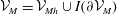 ${\mathcal{V}}_{M}={\mathcal{V}}_{Mh}\cup I(\unicode[STIX]{x2202}{\mathcal{V}}_{M})$
. (b) Position vectors associated with the averaging volume.
${\mathcal{V}}_{M}={\mathcal{V}}_{Mh}\cup I(\unicode[STIX]{x2202}{\mathcal{V}}_{M})$
. (b) Position vectors associated with the averaging volume.
2 Pore-scale model
The development starts with the classical mass and momentum Navier–Stokes equations describing flow of a single Newtonian and incompressible fluid phase
 $\unicode[STIX]{x1D6FD}$
that saturates the void space of a porous medium whose skeleton is made of a non-deformable solid phase
$\unicode[STIX]{x1D6FD}$
that saturates the void space of a porous medium whose skeleton is made of a non-deformable solid phase
 $\unicode[STIX]{x1D70E}$
such as the one sketched in figure 1(a). At any point in the pore space occupied by the
$\unicode[STIX]{x1D70E}$
such as the one sketched in figure 1(a). At any point in the pore space occupied by the
 $\unicode[STIX]{x1D6FD}$
-phase,
$\unicode[STIX]{x1D6FD}$
-phase,
 ${\mathcal{V}}_{\unicode[STIX]{x1D6FD},M}$
, and at any instant, these equations are given by
${\mathcal{V}}_{\unicode[STIX]{x1D6FD},M}$
, and at any instant, these equations are given by
 $$\begin{eqnarray}\displaystyle & \displaystyle \unicode[STIX]{x1D735}\boldsymbol{\cdot }\boldsymbol{v}_{\unicode[STIX]{x1D6FD}M}=0,\quad \text{in }{\mathcal{V}}_{\unicode[STIX]{x1D6FD},M},~t>0, & \displaystyle\end{eqnarray}$$
 $$\begin{eqnarray}\displaystyle & \displaystyle \unicode[STIX]{x1D70C}\left(\frac{\unicode[STIX]{x2202}\boldsymbol{v}_{\unicode[STIX]{x1D6FD}M}}{\unicode[STIX]{x2202}t}+\boldsymbol{v}_{\unicode[STIX]{x1D6FD}M}\boldsymbol{\cdot }\unicode[STIX]{x1D735}\boldsymbol{v}_{\unicode[STIX]{x1D6FD}M}\right)=-\unicode[STIX]{x1D735}p_{\unicode[STIX]{x1D6FD}M}+\unicode[STIX]{x1D70C}\boldsymbol{b}+\unicode[STIX]{x1D707}\unicode[STIX]{x1D6FB}^{2}\boldsymbol{v}_{\unicode[STIX]{x1D6FD}M},\quad \text{in }{\mathcal{V}}_{\unicode[STIX]{x1D6FD},M},~t>0, & \displaystyle\end{eqnarray}$$
where
 $p_{\unicode[STIX]{x1D6FD}M}$
and
$p_{\unicode[STIX]{x1D6FD}M}$
and
 $\boldsymbol{v}_{\unicode[STIX]{x1D6FD}M}$
are the fluid pressure and velocity, respectively;
$\boldsymbol{v}_{\unicode[STIX]{x1D6FD}M}$
are the fluid pressure and velocity, respectively;
 $t$
denotes time,
$t$
denotes time,
 $\unicode[STIX]{x1D70C}\boldsymbol{b}$
is the body force per unit volume,
$\unicode[STIX]{x1D70C}\boldsymbol{b}$
is the body force per unit volume,
 $\boldsymbol{b}$
being space-independent (but eventually time-varying), while
$\boldsymbol{b}$
being space-independent (but eventually time-varying), while
 $\unicode[STIX]{x1D70C}$
and
$\unicode[STIX]{x1D70C}$
and
 $\unicode[STIX]{x1D707}$
represent the density and dynamic viscosity of the fluid, respectively, which are considered constants. Furthermore, the no-slip boundary condition is enforced at the fixed solid–fluid interface,
$\unicode[STIX]{x1D707}$
represent the density and dynamic viscosity of the fluid, respectively, which are considered constants. Furthermore, the no-slip boundary condition is enforced at the fixed solid–fluid interface,
 ${\mathcal{A}}_{\unicode[STIX]{x1D6FD}\unicode[STIX]{x1D70E},M}$
,
${\mathcal{A}}_{\unicode[STIX]{x1D6FD}\unicode[STIX]{x1D70E},M}$
,
 $$\begin{eqnarray}\boldsymbol{v}_{\unicode[STIX]{x1D6FD}M}=\mathbf{0},\quad \text{at }{\mathcal{A}}_{\unicode[STIX]{x1D6FD}\unicode[STIX]{x1D70E},M},~t\geqslant 0.\end{eqnarray}$$
In addition, the velocity or the pressure at the macroscopic boundaries,
 ${\mathcal{A}}_{\unicode[STIX]{x1D6FD},M}$
, is assumed to be known and can be expressed as
${\mathcal{A}}_{\unicode[STIX]{x1D6FD},M}$
, is assumed to be known and can be expressed as
 $$\begin{eqnarray}\boldsymbol{v}_{\unicode[STIX]{x1D6FD}M}=\boldsymbol{v}_{in}\quad \text{or}\quad p_{\unicode[STIX]{x1D6FD}M}=p_{in},\quad \text{at }{\mathcal{A}}_{\unicode[STIX]{x1D6FD},M},~t>0.\end{eqnarray}$$
Finally, the corresponding initial condition is given by
 $$\begin{eqnarray}\boldsymbol{v}_{\unicode[STIX]{x1D6FD}M}=\boldsymbol{v}_{0},\quad \text{when }t=0,\quad \text{in }{\mathcal{V}}_{\unicode[STIX]{x1D6FD},M}.\end{eqnarray}$$
It is worth mentioning that, in general, measurements of
 $\boldsymbol{v}_{in}$
(or
$\boldsymbol{v}_{in}$
(or
 $p_{in}$
) and
$p_{in}$
) and
 $\boldsymbol{v}_{0}$
are not easily obtained but, nonetheless, for the development that follows, it is assumed that this information is available. However, as will be shown in the next paragraphs, not all of this information is actually required in the final upscaled model.
$\boldsymbol{v}_{0}$
are not easily obtained but, nonetheless, for the development that follows, it is assumed that this information is available. However, as will be shown in the next paragraphs, not all of this information is actually required in the final upscaled model.
3 Averaging
On the basis of the above-stated initial boundary value problem, the purpose of the analysis is to derive a macroscopic unsteady flow model including inertia. To this end, an upscaling procedure must be applied. Among techniques like homogenization (Auriault, Boutin & Geindreau Reference Auriault, Boutin and Geindreau2009) or the thermodynamically constrained averaging technique (Gray & Miller Reference Gray and Miller2014) and many others (Cushman, Bennethum & Hu Reference Cushman, Bennethum and Hu2002), the method of volume averaging (Whitaker Reference Whitaker1999) is retained in this work. In order to spatially smooth the pore-scale heterogeneities, it is necessary to introduce an averaging operator, which can be applied to the field of any piecewise continuous function,
 $\unicode[STIX]{x1D713}$
, defined everywhere in the
$\unicode[STIX]{x1D713}$
, defined everywhere in the
 $\unicode[STIX]{x1D6FD}$
-phase as
$\unicode[STIX]{x1D6FD}$
-phase as
 $$\begin{eqnarray}\langle \unicode[STIX]{x1D713}\rangle |_{\boldsymbol{x},t}=\frac{1}{V}\int _{{\mathcal{V}}_{\unicode[STIX]{x1D6FD}}(\boldsymbol{x})}\unicode[STIX]{x1D713}(\boldsymbol{r},t)\,\text{d}V,\end{eqnarray}$$
where the position vector
 $\boldsymbol{x}$
locates the centroid of the averaging domain, whereas
$\boldsymbol{x}$
locates the centroid of the averaging domain, whereas
 $\boldsymbol{y}$
and
$\boldsymbol{y}$
and
 $\boldsymbol{r}=\boldsymbol{y}\,+\,\boldsymbol{x}$
locate points within the
$\boldsymbol{r}=\boldsymbol{y}\,+\,\boldsymbol{x}$
locate points within the
 $\unicode[STIX]{x1D6FD}$
-phase with respect to
$\unicode[STIX]{x1D6FD}$
-phase with respect to
 $\boldsymbol{x}$
and a fixed coordinate system, respectively, as indicated in figure 1(b). In the above expression,
$\boldsymbol{x}$
and a fixed coordinate system, respectively, as indicated in figure 1(b). In the above expression,
 ${\mathcal{V}}$
denotes the averaging volume of measure
${\mathcal{V}}$
denotes the averaging volume of measure
 $V$
and radius
$V$
and radius
 $r_{0}$
(see figure 1
a). The averaging operator defined in (3.1a
) is usually denoted as the superficial averaging operator (Whitaker Reference Whitaker1999), a nomenclature that is employed throughout the article. In addition, the intrinsic averaging operator is defined as
$r_{0}$
(see figure 1
a). The averaging operator defined in (3.1a
) is usually denoted as the superficial averaging operator (Whitaker Reference Whitaker1999), a nomenclature that is employed throughout the article. In addition, the intrinsic averaging operator is defined as
 $$\begin{eqnarray}\langle \unicode[STIX]{x1D713}\rangle ^{\unicode[STIX]{x1D6FD}}|_{\boldsymbol{x},t}=\frac{1}{V_{\unicode[STIX]{x1D6FD}}(\boldsymbol{x})}\int _{{\mathcal{V}}_{\unicode[STIX]{x1D6FD}}(\boldsymbol{x})}\unicode[STIX]{x1D713}(\boldsymbol{r},t)\,\text{d}V,\end{eqnarray}$$
where
 $V_{\unicode[STIX]{x1D6FD}}(\boldsymbol{x})$
represents the volume of the
$V_{\unicode[STIX]{x1D6FD}}(\boldsymbol{x})$
represents the volume of the
 $\unicode[STIX]{x1D6FD}$
-phase within
$\unicode[STIX]{x1D6FD}$
-phase within
 ${\mathcal{V}}$
. The superficial and intrinsic averaging operators are related by the Dupuit–Forchheimer relationship
${\mathcal{V}}$
. The superficial and intrinsic averaging operators are related by the Dupuit–Forchheimer relationship
 $$\begin{eqnarray}\langle \unicode[STIX]{x1D713}\rangle |_{\boldsymbol{x},t}=\unicode[STIX]{x1D700}(\boldsymbol{x})\langle \unicode[STIX]{x1D713}\rangle ^{\unicode[STIX]{x1D6FD}}|_{\boldsymbol{x},t},\end{eqnarray}$$
with
 $\unicode[STIX]{x1D700}(\boldsymbol{x})\equiv V_{\unicode[STIX]{x1D6FD}}(\boldsymbol{x})/V$
denoting the porosity, which is a constant due to the rigid and homogeneous character of the medium. To facilitate the notation, subscripts
$\unicode[STIX]{x1D700}(\boldsymbol{x})\equiv V_{\unicode[STIX]{x1D6FD}}(\boldsymbol{x})/V$
denoting the porosity, which is a constant due to the rigid and homogeneous character of the medium. To facilitate the notation, subscripts
 $\boldsymbol{x}$
and
$\boldsymbol{x}$
and
 $t$
will be omitted in the remainder of the article.
$t$
will be omitted in the remainder of the article.
While carrying out the analysis, the general transport theorem (Truesdell & Toupin Reference Truesdell and Toupin1960; Slattery Reference Slattery1999) and the spatial averaging theorem (Howes & Whitaker Reference Howes and Whitaker1985) will be employed. They are respectively given by
 $$\begin{eqnarray}\displaystyle \left\langle \frac{\unicode[STIX]{x2202}\unicode[STIX]{x1D713}}{\unicode[STIX]{x2202}t}\right\rangle & = & \displaystyle \frac{\unicode[STIX]{x2202}\langle \unicode[STIX]{x1D713}\rangle }{\unicode[STIX]{x2202}t}-\frac{1}{V}\int _{{\mathcal{A}}_{\unicode[STIX]{x1D6FD}\unicode[STIX]{x1D70E}}}\boldsymbol{n}\boldsymbol{\cdot }\boldsymbol{w}\unicode[STIX]{x1D713}\,\text{d}A,\end{eqnarray}$$
 $$\begin{eqnarray}\displaystyle \langle \unicode[STIX]{x1D735}\unicode[STIX]{x1D713}\rangle & = & \displaystyle \unicode[STIX]{x1D735}\langle \unicode[STIX]{x1D713}\rangle +\frac{1}{V}\int _{{\mathcal{A}}_{\unicode[STIX]{x1D6FD}\unicode[STIX]{x1D70E}}}\boldsymbol{n}\unicode[STIX]{x1D713}\,\text{d}A.\end{eqnarray}$$
In the equations above,
 $\boldsymbol{n}$
is the unit normal vector at
$\boldsymbol{n}$
is the unit normal vector at
 ${\mathcal{A}}_{\unicode[STIX]{x1D6FD}\unicode[STIX]{x1D70E}}$
directed from the
${\mathcal{A}}_{\unicode[STIX]{x1D6FD}\unicode[STIX]{x1D70E}}$
directed from the
 $\unicode[STIX]{x1D6FD}$
-phase towards the
$\unicode[STIX]{x1D6FD}$
-phase towards the
 $\unicode[STIX]{x1D70E}$
-phase as indicated in figure 1(a) and
$\unicode[STIX]{x1D70E}$
-phase as indicated in figure 1(a) and
 $\boldsymbol{w}$
denotes the displacement velocity of
$\boldsymbol{w}$
denotes the displacement velocity of
 ${\mathcal{A}}_{\unicode[STIX]{x1D6FD}\unicode[STIX]{x1D70E}}$
. Because the porous medium is assumed to be rigid,
${\mathcal{A}}_{\unicode[STIX]{x1D6FD}\unicode[STIX]{x1D70E}}$
. Because the porous medium is assumed to be rigid,
 $\boldsymbol{w}=\mathbf{0}$
and, together with the fact that the structure is homogeneous, the above theorems may be rewritten in terms of intrinsic averages as follows:
$\boldsymbol{w}=\mathbf{0}$
and, together with the fact that the structure is homogeneous, the above theorems may be rewritten in terms of intrinsic averages as follows:
 $$\begin{eqnarray}\displaystyle \left\langle \frac{\unicode[STIX]{x2202}\unicode[STIX]{x1D713}}{\unicode[STIX]{x2202}t}\right\rangle ^{\unicode[STIX]{x1D6FD}} & = & \displaystyle \frac{\unicode[STIX]{x2202}\langle \unicode[STIX]{x1D713}\rangle ^{\unicode[STIX]{x1D6FD}}}{\unicode[STIX]{x2202}t},\end{eqnarray}$$
 $$\begin{eqnarray}\displaystyle \langle \unicode[STIX]{x1D735}\unicode[STIX]{x1D713}\rangle ^{\unicode[STIX]{x1D6FD}} & = & \displaystyle \unicode[STIX]{x1D735}\langle \unicode[STIX]{x1D713}\rangle ^{\unicode[STIX]{x1D6FD}}+\frac{1}{V_{\unicode[STIX]{x1D6FD}}}\int _{{\mathcal{A}}_{\unicode[STIX]{x1D6FD}\unicode[STIX]{x1D70E}}}\boldsymbol{n}\unicode[STIX]{x1D713}\,\text{d}A.\end{eqnarray}$$
As for any upscaling technique, a scale hierarchy is assumed as a prerequisite, namely a separation of characteristic length scales that can be stated as
 $$\begin{eqnarray}\ell _{\unicode[STIX]{x1D6FD}}\ll r_{0}\ll L,\end{eqnarray}$$
where
 $\ell _{\unicode[STIX]{x1D6FD}}$
represents the characteristic pore length scale and
$\ell _{\unicode[STIX]{x1D6FD}}$
represents the characteristic pore length scale and
 $L$
the size of the macroscopic domain.
$L$
the size of the macroscopic domain.
In order to derive a model that is expressed only in terms of macroscopic quantities, it is convenient to introduce the following spatial decomposition (Gray Reference Gray1975)
 $$\begin{eqnarray}\unicode[STIX]{x1D713}=\langle \unicode[STIX]{x1D713}\rangle ^{\unicode[STIX]{x1D6FD}}+\tilde{\unicode[STIX]{x1D713}},\quad \unicode[STIX]{x1D713}=\boldsymbol{v},p.\end{eqnarray}$$
This decomposition is intended to operate a spatial length-scale decoupling as the deviation field,
 $\tilde{\unicode[STIX]{x1D713}}$
, is expected to vary at the scale
$\tilde{\unicode[STIX]{x1D713}}$
, is expected to vary at the scale
 $\ell _{\unicode[STIX]{x1D6FD}}$
while the intrinsic average,
$\ell _{\unicode[STIX]{x1D6FD}}$
while the intrinsic average,
 $\langle \unicode[STIX]{x1D713}\rangle ^{\unicode[STIX]{x1D6FD}}$
, experiences significant variations at the scale
$\langle \unicode[STIX]{x1D713}\rangle ^{\unicode[STIX]{x1D6FD}}$
, experiences significant variations at the scale
 $L$
. This contrast can be clearly established at steady state and, for the dynamic flow process under consideration, it is assumed that this condition is satisfied at any time. As a consequence of the scale hierarchy expressed in (3.5),
$L$
. This contrast can be clearly established at steady state and, for the dynamic flow process under consideration, it is assumed that this condition is satisfied at any time. As a consequence of the scale hierarchy expressed in (3.5),
 $\langle \unicode[STIX]{x1D713}\rangle ^{\unicode[STIX]{x1D6FD}}$
can be treated as a constant at all times within the averaging volume (Whitaker Reference Whitaker1999), with the consequence that
$\langle \unicode[STIX]{x1D713}\rangle ^{\unicode[STIX]{x1D6FD}}$
can be treated as a constant at all times within the averaging volume (Whitaker Reference Whitaker1999), with the consequence that
 $$\begin{eqnarray}\langle \tilde{\unicode[STIX]{x1D713}}\rangle ^{\unicode[STIX]{x1D6FD}}\simeq 0.\end{eqnarray}$$

Figure 2. Two-dimensional sketch of a periodic structure and a geometrical periodic unit cell of side length
 $\ell$
.
$\ell$
.
The development of the macroscopic model is now carried out considering that the porous medium is periodic, which represents a classical hypothesis in upscaling methods. Under these circumstances, it is sufficient to consider the above-stated initial boundary value problem (2.1) over a periodic unit cell that will correspond to the averaging volume
 ${\mathcal{V}}$
. Here, special attention should be paid to the fact that, for unsteady flow, this periodic unit cell may not necessarily coincide with the geometrical one depicted in figure 2. This was highlighted in the study of the first Hopf bifurcation in model periodic structures in the work by Agnaou, Lasseux & Ahmadi (Reference Agnaou, Lasseux and Ahmadi2016).
${\mathcal{V}}$
. Here, special attention should be paid to the fact that, for unsteady flow, this periodic unit cell may not necessarily coincide with the geometrical one depicted in figure 2. This was highlighted in the study of the first Hopf bifurcation in model periodic structures in the work by Agnaou, Lasseux & Ahmadi (Reference Agnaou, Lasseux and Ahmadi2016).
3.1 Formal solution in a unit cell
With the above at our disposal, the analysis can be directed to the homogeneous part
 ${\mathcal{V}}_{Mh}$
of the entire domain, i.e. excluding the region
${\mathcal{V}}_{Mh}$
of the entire domain, i.e. excluding the region
 $I(\unicode[STIX]{x2202}{\mathcal{V}}_{M})$
near the macroscopic boundary of the system. A development similar to that reported by Whitaker (Reference Whitaker1996) may be followed to reach a macroscopic model involving only the average velocity and pressure. However, following the idea used in Barrere, Gipouloux & Whitaker (Reference Barrere, Gipouloux and Whitaker1992, § 2), a shorter alternative procedure, which basically consists of expressing the formal solution of the pore-scale initial boundary value problem over a periodic unit cell in terms of the driving forces, followed by an averaging step, may be adopted to considerably simplify the development. The use of periodicity is more a convenience than a necessity, since the same procedure can be adopted without this restriction. This approach is consistent with the assumption of separation of length scales in the homogeneous region of the porous medium. With this in mind, the pore-scale problem in (2.1) is rewritten in a periodic unit cell in terms of the dependent variables
$I(\unicode[STIX]{x2202}{\mathcal{V}}_{M})$
near the macroscopic boundary of the system. A development similar to that reported by Whitaker (Reference Whitaker1996) may be followed to reach a macroscopic model involving only the average velocity and pressure. However, following the idea used in Barrere, Gipouloux & Whitaker (Reference Barrere, Gipouloux and Whitaker1992, § 2), a shorter alternative procedure, which basically consists of expressing the formal solution of the pore-scale initial boundary value problem over a periodic unit cell in terms of the driving forces, followed by an averaging step, may be adopted to considerably simplify the development. The use of periodicity is more a convenience than a necessity, since the same procedure can be adopted without this restriction. This approach is consistent with the assumption of separation of length scales in the homogeneous region of the porous medium. With this in mind, the pore-scale problem in (2.1) is rewritten in a periodic unit cell in terms of the dependent variables
 $\boldsymbol{v}$
and
$\boldsymbol{v}$
and
 $p$
. Unlike
$p$
. Unlike
 $\boldsymbol{v}$
,
$\boldsymbol{v}$
,
 $p$
is not a periodic field, but the decomposition provided in (3.6) should be used so that
$p$
is not a periodic field, but the decomposition provided in (3.6) should be used so that
 $\tilde{p}$
is periodic, yielding
$\tilde{p}$
is periodic, yielding
 $$\begin{eqnarray}\displaystyle & \displaystyle \unicode[STIX]{x1D735}\boldsymbol{\cdot }\boldsymbol{v}=0,\quad \text{in }{\mathcal{V}}_{\unicode[STIX]{x1D6FD}},~t>0, & \displaystyle\end{eqnarray}$$
 $$\begin{eqnarray}\displaystyle & \displaystyle \unicode[STIX]{x1D70C}\left(\frac{\unicode[STIX]{x2202}\boldsymbol{v}}{\unicode[STIX]{x2202}t}+\boldsymbol{v}\boldsymbol{\cdot }\unicode[STIX]{x1D735}\boldsymbol{v}\right)=-\unicode[STIX]{x1D735}\tilde{p}+\unicode[STIX]{x1D707}\unicode[STIX]{x1D6FB}^{2}\boldsymbol{v}+\underbrace{(-\unicode[STIX]{x1D735}\langle p\rangle ^{\unicode[STIX]{x1D6FD}}+\unicode[STIX]{x1D70C}\boldsymbol{b})}_{source},\quad \text{in }{\mathcal{V}}_{\unicode[STIX]{x1D6FD}},~t>0, & \displaystyle\end{eqnarray}$$
 $$\begin{eqnarray}\displaystyle & \displaystyle \boldsymbol{v}=\mathbf{0},\quad \text{at }{\mathcal{A}}_{\unicode[STIX]{x1D6FD}\unicode[STIX]{x1D70E}},~t\geqslant 0, & \displaystyle\end{eqnarray}$$
 $$\begin{eqnarray}\displaystyle & \displaystyle \boldsymbol{v}=\underbrace{\boldsymbol{v}_{0}}_{source},\quad \text{in }{\mathcal{V}}_{\unicode[STIX]{x1D6FD}},\quad \text{when }t=0, & \displaystyle\end{eqnarray}$$
 $$\begin{eqnarray}\displaystyle & \displaystyle \langle \tilde{p}\rangle ^{\unicode[STIX]{x1D6FD}}=0,~t>0, & \displaystyle\end{eqnarray}$$
 $$\begin{eqnarray}\displaystyle & \displaystyle \boldsymbol{v}(\boldsymbol{r}+\boldsymbol{l}_{i})=\boldsymbol{v}(\boldsymbol{r}),\quad \tilde{p}(\boldsymbol{r}+\boldsymbol{l}_{i})=\tilde{p}(\boldsymbol{r}),\quad t>0,\quad i=1,2,3, & \displaystyle\end{eqnarray}$$
 ${\mathcal{V}}_{\unicode[STIX]{x1D6FD}}$
and
${\mathcal{V}}_{\unicode[STIX]{x1D6FD}}$
and
 $A_{\unicode[STIX]{x1D6FD}\unicode[STIX]{x1D70E}}$
, respectively, designate the region occupied by the
$A_{\unicode[STIX]{x1D6FD}\unicode[STIX]{x1D70E}}$
, respectively, designate the region occupied by the
 $\unicode[STIX]{x1D6FD}$
-phase and the solid–fluid interface within the unit cell of periodic lattice vectors
$\unicode[STIX]{x1D6FD}$
-phase and the solid–fluid interface within the unit cell of periodic lattice vectors
 $\boldsymbol{l}_{i}$
. Note that (3.8e
) and (3.8f
) replace the external boundary condition in (2.1d,e
).
$\boldsymbol{l}_{i}$
. Note that (3.8e
) and (3.8f
) replace the external boundary condition in (2.1d,e
). The nonlinear character of the above problem makes a formal solution very difficult to obtain and, for this reason, a linearization approach is of interest. Indeed, a solution at time
 $t$
can be sought assuming that the convective velocity exists and is available at a time
$t$
can be sought assuming that the convective velocity exists and is available at a time
 $t-\unicode[STIX]{x0394}t$
, for any small enough value of
$t-\unicode[STIX]{x0394}t$
, for any small enough value of
 $\unicode[STIX]{x0394}t$
. Under these circumstances, the momentum equation (3.8b
) can be approximated using a zeroth-order Taylor expansion in time, leading to the approximation
$\unicode[STIX]{x0394}t$
. Under these circumstances, the momentum equation (3.8b
) can be approximated using a zeroth-order Taylor expansion in time, leading to the approximation
 $\boldsymbol{v}|_{t}\approx \boldsymbol{v}|_{t-\unicode[STIX]{x0394}t}\equiv \boldsymbol{v}_{\unicode[STIX]{x1D6E5}}$
. In this way, equation (3.8b
) takes the form
$\boldsymbol{v}|_{t}\approx \boldsymbol{v}|_{t-\unicode[STIX]{x0394}t}\equiv \boldsymbol{v}_{\unicode[STIX]{x1D6E5}}$
. In this way, equation (3.8b
) takes the form
 $$\begin{eqnarray}\unicode[STIX]{x1D70C}\left(\frac{\unicode[STIX]{x2202}\boldsymbol{v}}{\unicode[STIX]{x2202}t}+\boldsymbol{v}_{\unicode[STIX]{x1D6E5}}\boldsymbol{\cdot }\unicode[STIX]{x1D735}\boldsymbol{v}\right)=-\unicode[STIX]{x1D735}\tilde{p}+\unicode[STIX]{x1D707}\unicode[STIX]{x1D6FB}^{2}\boldsymbol{v}+\underbrace{(-\unicode[STIX]{x1D735}\langle p\rangle ^{\unicode[STIX]{x1D6FD}}+\unicode[STIX]{x1D70C}\boldsymbol{b})}_{source},\quad \text{in }{\mathcal{V}}_{\unicode[STIX]{x1D6FD}},~t>0.\end{eqnarray}$$
This type of approximation is a consistent one and is typical in a numerical approach consisting of a linearization of the convective term that makes use of an explicit form of the convective velocity. As will be shown later, the information about the time step and the rest of the terms of the Taylor expansion in time are ultimately not required in the resulting closure problems. With the momentum balance in the form of (3.9), the initial and boundary value problem is a linear one for which a formal solution can be obtained using an integral equation formulation in terms of Green’s functions as shown by Wood & Valdés-Parada (Reference Wood and Valdés-Parada2013). This solution can be written as
 $$\begin{eqnarray}\displaystyle & \displaystyle \boldsymbol{v}=\frac{1}{\unicode[STIX]{x1D707}}\left(\frac{\unicode[STIX]{x2202}\unicode[STIX]{x1D63F}}{\unicode[STIX]{x2202}t}\,\ast \boldsymbol{\cdot }\,(-\unicode[STIX]{x1D735}\langle p\rangle ^{\unicode[STIX]{x1D6FD}}+\unicode[STIX]{x1D70C}\boldsymbol{b})+\boldsymbol{m}_{0}\right),\quad \text{in }{\mathcal{V}}_{\unicode[STIX]{x1D6FD}},~t>0, & \displaystyle\end{eqnarray}$$
 $$\begin{eqnarray}\displaystyle & \displaystyle \tilde{p}=\frac{\unicode[STIX]{x2202}\boldsymbol{d}}{\unicode[STIX]{x2202}t}\,\ast \boldsymbol{\cdot }\,(-\unicode[STIX]{x1D735}\langle p\rangle ^{\unicode[STIX]{x1D6FD}}+\unicode[STIX]{x1D70C}\boldsymbol{b})+n_{0},\quad \text{in }{\mathcal{V}}_{\unicode[STIX]{x1D6FD}},~t>0. & \displaystyle\end{eqnarray}$$
 $\ast \boldsymbol{\cdot }$
is adopted to denote the combined convolution and dot products. For two time-dependent tensors of any order,
$\ast \boldsymbol{\cdot }$
is adopted to denote the combined convolution and dot products. For two time-dependent tensors of any order,
 $\unicode[STIX]{x1D73F}_{1}$
and
$\unicode[STIX]{x1D73F}_{1}$
and
 $\unicode[STIX]{x1D73F}_{2}$
, this product is given by
$\unicode[STIX]{x1D73F}_{2}$
, this product is given by  $$\begin{eqnarray}\unicode[STIX]{x1D73F}_{1}\,\ast \boldsymbol{\cdot }\,\unicode[STIX]{x1D73F}_{2}=\int _{t_{0}=0}^{t_{0}=t}\unicode[STIX]{x1D73F}_{1}|_{t-t_{0}}\boldsymbol{\cdot }\unicode[STIX]{x1D73F}_{2}|_{t_{0}}\,\text{d}t_{0}=\int _{t_{0}=0}^{t_{0}=t}\unicode[STIX]{x1D73F}_{1}|_{t_{0}}\boldsymbol{\cdot }\unicode[STIX]{x1D73F}_{2}|_{t-t_{0}}\,\text{d}t_{0}.\end{eqnarray}$$
While writing the representations in (3.10), it is meant that
 $\unicode[STIX]{x2202}\unicode[STIX]{x1D63F}/\unicode[STIX]{x2202}t$
(respectively
$\unicode[STIX]{x2202}\unicode[STIX]{x1D63F}/\unicode[STIX]{x2202}t$
(respectively
 $\unicode[STIX]{x2202}\boldsymbol{d}/\unicode[STIX]{x2202}t$
) is the closure variable that maps
$\unicode[STIX]{x2202}\boldsymbol{d}/\unicode[STIX]{x2202}t$
) is the closure variable that maps
 $(-\unicode[STIX]{x1D735}\langle p\rangle ^{\unicode[STIX]{x1D6FD}}+\unicode[STIX]{x1D70C}\boldsymbol{b})$
onto
$(-\unicode[STIX]{x1D735}\langle p\rangle ^{\unicode[STIX]{x1D6FD}}+\unicode[STIX]{x1D70C}\boldsymbol{b})$
onto
 $\boldsymbol{v}$
(respectively
$\boldsymbol{v}$
(respectively
 $\tilde{p}$
) while
$\tilde{p}$
) while
 $\boldsymbol{m}_{0}$
(respectively
$\boldsymbol{m}_{0}$
(respectively
 $n_{0}$
) is the closure variable that maps
$n_{0}$
) is the closure variable that maps
 $\boldsymbol{v}_{0}$
onto
$\boldsymbol{v}_{0}$
onto
 $\boldsymbol{v}$
(respectively
$\boldsymbol{v}$
(respectively
 $\tilde{p}$
). At this point, it is worth mentioning that the initial conditions for
$\tilde{p}$
). At this point, it is worth mentioning that the initial conditions for
 $\unicode[STIX]{x1D63F}$
and
$\unicode[STIX]{x1D63F}$
and
 $\boldsymbol{d}$
yield unique solutions that are driven by the sources, as will be provided later in the derivations.
$\boldsymbol{d}$
yield unique solutions that are driven by the sources, as will be provided later in the derivations.
It must be mentioned that the formal solution given in (3.10) does not correspond, except when
 $\boldsymbol{v}_{0}=\mathbf{0}$
, to the one reported by Lions (Reference Lions1981) (see (5.20) therein), under creeping flow conditions, and by Mikelić (Reference Mikelić1994) (see equation (P) therein for the creeping regime solution and the ‘Proof of Theorem 1.4’ in § 2.4 for the inertial case solution in the Laplace domain). The difference lies in the fact that these authors considered the initial condition to be a function only of
$\boldsymbol{v}_{0}=\mathbf{0}$
, to the one reported by Lions (Reference Lions1981) (see (5.20) therein), under creeping flow conditions, and by Mikelić (Reference Mikelić1994) (see equation (P) therein for the creeping regime solution and the ‘Proof of Theorem 1.4’ in § 2.4 for the inertial case solution in the Laplace domain). The difference lies in the fact that these authors considered the initial condition to be a function only of
 $\boldsymbol{x}$
as proposed in (5.10) of chap. 2 in Lions (Reference Lions1981). Note that this assumption is physically questionable and it is not retained in the present work just as it was not considered by Allaire (Reference Allaire1992) for the study of unsteady creeping flow in porous media.
$\boldsymbol{x}$
as proposed in (5.10) of chap. 2 in Lions (Reference Lions1981). Note that this assumption is physically questionable and it is not retained in the present work just as it was not considered by Allaire (Reference Allaire1992) for the study of unsteady creeping flow in porous media.
The macroscopic mass and momentum conservation equations can now be obtained by applying the superficial averaging operator on (3.8a ) and (3.10a ), respectively. In order to obtain the macroscale mass conservation equation, it is also necessary to make use of the averaging theorem, together with the no-slip boundary condition, leading to
 $$\begin{eqnarray}\unicode[STIX]{x1D735}\boldsymbol{\cdot }\langle \boldsymbol{v}\rangle =0,\quad \text{in }{\mathcal{V}}_{Mh},~t>0.\end{eqnarray}$$
In addition, the macroscale filtration velocity equation is given by
 $$\begin{eqnarray}\langle \boldsymbol{v}\rangle =-\frac{1}{\unicode[STIX]{x1D707}}\left(\frac{\unicode[STIX]{x2202}\langle \unicode[STIX]{x1D63F}\rangle }{\unicode[STIX]{x2202}t}\,\ast \boldsymbol{\cdot }\,(\unicode[STIX]{x1D735}\langle p\rangle ^{\unicode[STIX]{x1D6FD}}-\unicode[STIX]{x1D70C}\boldsymbol{b})-\langle \boldsymbol{m}_{0}\rangle \right),\quad \text{in }{\mathcal{V}}_{Mh},~t>0.\end{eqnarray}$$
Here, the assumption that
 $\unicode[STIX]{x1D735}\langle p\rangle ^{\unicode[STIX]{x1D6FD}}$
can be considered as a constant within
$\unicode[STIX]{x1D735}\langle p\rangle ^{\unicode[STIX]{x1D6FD}}$
can be considered as a constant within
 ${\mathcal{V}}$
was taken into account. The effective coefficients
${\mathcal{V}}$
was taken into account. The effective coefficients
 $\langle \unicode[STIX]{x1D63F}\rangle$
and
$\langle \unicode[STIX]{x1D63F}\rangle$
and
 $\langle \boldsymbol{m}_{0}\rangle$
are determined by solving the closure problems detailed in the following section. Comments about the physics of the upscaled model and its coefficients are also provided below, together with some remarks on the existing related literature.
$\langle \boldsymbol{m}_{0}\rangle$
are determined by solving the closure problems detailed in the following section. Comments about the physics of the upscaled model and its coefficients are also provided below, together with some remarks on the existing related literature.
3.2 Closure problems and macroscopic model
Substitution of the formal solution given in (3.10) into the initial boundary value problem in (3.8) and separating the contributions from the two sources, while maintaining the convolution product with the volume source, leads to the following equations for
 $\unicode[STIX]{x1D63F}$
and
$\unicode[STIX]{x1D63F}$
and
 $\boldsymbol{d}$
:
$\boldsymbol{d}$
:
 $$\begin{eqnarray}\displaystyle & & \displaystyle \int _{t_{0}=0}^{t_{0}=t}\left(\unicode[STIX]{x1D735}\cdot \left.\frac{\unicode[STIX]{x2202}\unicode[STIX]{x1D63F}}{\unicode[STIX]{x2202}t}\right|_{t-t_{0}}\right)\boldsymbol{\cdot }(-\unicode[STIX]{x1D735}\langle p\rangle ^{\unicode[STIX]{x1D6FD}}+\unicode[STIX]{x1D70C}\boldsymbol{b})_{t_{0}}\,\text{d}t_{0}=\mathbf{0},\quad \text{in }{\mathcal{V}}_{\unicode[STIX]{x1D6FD}},~t>0,\end{eqnarray}$$
 $$\begin{eqnarray}\displaystyle & & \displaystyle \int _{t_{0}=0}^{t_{0}=t}\left[\frac{\unicode[STIX]{x1D70C}}{\unicode[STIX]{x1D707}}\left(\left.\frac{\unicode[STIX]{x2202}^{2}\unicode[STIX]{x1D63F}}{\unicode[STIX]{x2202}t^{2}}\right|_{t-t_{0}}+\boldsymbol{v}_{\unicode[STIX]{x1D6E5}}\cdot \left.\frac{\unicode[STIX]{x2202}\unicode[STIX]{x1D735}\unicode[STIX]{x1D63F}}{\unicode[STIX]{x2202}t}\right|_{t-t_{0}}\right)+\left.\frac{\unicode[STIX]{x2202}\unicode[STIX]{x1D735}\boldsymbol{d}}{\unicode[STIX]{x2202}t}\right|_{t-t_{0}}-\left.\frac{\unicode[STIX]{x2202}\unicode[STIX]{x1D6FB}^{2}\unicode[STIX]{x1D63F}}{\unicode[STIX]{x2202}t}\right|_{t-t_{0}}-\left.\unicode[STIX]{x1D644}\frac{\text{d}{\mathcal{H}}}{\text{d}t}\right|_{t-t_{0}}\right]\nonumber\\ \displaystyle & & \displaystyle \quad \cdot \,(-\unicode[STIX]{x1D735}\langle p\rangle ^{\unicode[STIX]{x1D6FD}}+\unicode[STIX]{x1D70C}\boldsymbol{b})_{t_{0}}\,\text{d}t_{0}=\mathbf{0},\quad \text{in }{\mathcal{V}}_{\unicode[STIX]{x1D6FD}},~t\geqslant 0,\end{eqnarray}$$
 $$\begin{eqnarray}\displaystyle & & \displaystyle \int _{t_{0}=0}^{t_{0}=t}\left.\frac{\unicode[STIX]{x2202}\unicode[STIX]{x1D63F}}{\unicode[STIX]{x2202}t}\right|_{t-t_{0}}\cdot (-\unicode[STIX]{x1D735}\langle p\rangle ^{\unicode[STIX]{x1D6FD}}+\unicode[STIX]{x1D70C}\boldsymbol{b})_{t_{0}}\,\text{d}t_{0}=\mathbf{0},\quad \text{at }{\mathcal{A}}_{\unicode[STIX]{x1D6FD}\unicode[STIX]{x1D70E}},~t\geqslant 0,\end{eqnarray}$$
 ${\mathcal{H}}$
represents the Heaviside function. These equations are completed with periodic boundary conditions for
${\mathcal{H}}$
represents the Heaviside function. These equations are completed with periodic boundary conditions for
 $\unicode[STIX]{x1D63F}$
and
$\unicode[STIX]{x1D63F}$
and
 $\boldsymbol{d}$
and
$\boldsymbol{d}$
and
 $\langle \unicode[STIX]{x2202}\boldsymbol{d}/\unicode[STIX]{x2202}t\rangle ^{\unicode[STIX]{x1D6FD}}=\mathbf{0}$
. Note that, at this point, the initial condition for the closure variables has not yet been defined.
$\langle \unicode[STIX]{x2202}\boldsymbol{d}/\unicode[STIX]{x2202}t\rangle ^{\unicode[STIX]{x1D6FD}}=\mathbf{0}$
. Note that, at this point, the initial condition for the closure variables has not yet been defined. In order to satisfy the above equations, valid for any macroscopic forcing
 $(-\unicode[STIX]{x1D735}\langle p\rangle ^{\unicode[STIX]{x1D6FD}}+\unicode[STIX]{x1D70C}\boldsymbol{b})$
and at any time,
$(-\unicode[STIX]{x1D735}\langle p\rangle ^{\unicode[STIX]{x1D6FD}}+\unicode[STIX]{x1D70C}\boldsymbol{b})$
and at any time,
 $\unicode[STIX]{x1D63F}$
and
$\unicode[STIX]{x1D63F}$
and
 $\boldsymbol{d}$
must satisfy the following equations, in general (this may be inferred from considering the particular case in which the macroscopic forcing is a constant):
$\boldsymbol{d}$
must satisfy the following equations, in general (this may be inferred from considering the particular case in which the macroscopic forcing is a constant):
 $$\begin{eqnarray}\displaystyle & \displaystyle \unicode[STIX]{x1D735}\boldsymbol{\cdot }\frac{\unicode[STIX]{x2202}\unicode[STIX]{x1D63F}}{\unicode[STIX]{x2202}t}=\mathbf{0},\quad \text{in }{\mathcal{V}}_{\unicode[STIX]{x1D6FD}},~t>0, & \displaystyle\end{eqnarray}$$
 $$\begin{eqnarray}\displaystyle & \displaystyle \frac{\unicode[STIX]{x1D70C}}{\unicode[STIX]{x1D707}}\left(\left.\frac{\unicode[STIX]{x2202}^{2}\unicode[STIX]{x1D63F}}{\unicode[STIX]{x2202}t^{2}}\right|_{\unicode[STIX]{x1D70F}}+\boldsymbol{v}\boldsymbol{\cdot }\left.\frac{\unicode[STIX]{x2202}\unicode[STIX]{x1D735}\unicode[STIX]{x1D63F}}{\unicode[STIX]{x2202}t}\right|_{\unicode[STIX]{x1D70F}}\right)+\left.\frac{\unicode[STIX]{x2202}\unicode[STIX]{x1D735}\boldsymbol{d}}{\unicode[STIX]{x2202}t}\right|_{\unicode[STIX]{x1D70F}}-\left.\frac{\unicode[STIX]{x2202}\unicode[STIX]{x1D6FB}^{2}\unicode[STIX]{x1D63F}}{\unicode[STIX]{x2202}t}\right|_{\unicode[STIX]{x1D70F}}-\unicode[STIX]{x1D644}\left.\frac{\text{d}{\mathcal{H}}}{\text{d}t}\right|_{\unicode[STIX]{x1D70F}}=\mathbf{0}, & \displaystyle \nonumber\\ \displaystyle & \displaystyle \qquad \text{in }{\mathcal{V}}_{\unicode[STIX]{x1D6FD}},\quad 0\leqslant \unicode[STIX]{x1D70F}\leqslant t,~t>0, & \displaystyle\end{eqnarray}$$
 $$\begin{eqnarray}\displaystyle & \displaystyle \frac{\unicode[STIX]{x2202}\unicode[STIX]{x1D63F}}{\unicode[STIX]{x2202}t}=\mathbf{0},\quad \text{at }{\mathcal{A}}_{\unicode[STIX]{x1D6FD}\unicode[STIX]{x1D70E}},~t>0, & \displaystyle\end{eqnarray}$$
 $\unicode[STIX]{x1D70F}$
denoting the elapsed time involved in the convolution product. Note that (3.14b
) is the result of taking the limit
$\unicode[STIX]{x1D70F}$
denoting the elapsed time involved in the convolution product. Note that (3.14b
) is the result of taking the limit
 $\unicode[STIX]{x0394}t\rightarrow 0$
, so that
$\unicode[STIX]{x0394}t\rightarrow 0$
, so that
 $\boldsymbol{v}_{\unicode[STIX]{x1D6E5}}\rightarrow \boldsymbol{v}$
. The value of the time step
$\boldsymbol{v}_{\unicode[STIX]{x1D6E5}}\rightarrow \boldsymbol{v}$
. The value of the time step
 $\unicode[STIX]{x1D6E5}$
and the information from the rest of the terms in the Taylor expansion in time is hence no longer required.
$\unicode[STIX]{x1D6E5}$
and the information from the rest of the terms in the Taylor expansion in time is hence no longer required. A subsequent time integration step of (3.14) from
 $\unicode[STIX]{x1D70F}=0$
to
$\unicode[STIX]{x1D70F}=0$
to
 $\unicode[STIX]{x1D70F}=t$
yields
$\unicode[STIX]{x1D70F}=t$
yields
 $$\begin{eqnarray}\displaystyle & \displaystyle \left[\unicode[STIX]{x1D735}\boldsymbol{\cdot }\unicode[STIX]{x1D63F}\right]_{\unicode[STIX]{x1D70F}=0}^{\unicode[STIX]{x1D70F}=t}=\mathbf{0},\quad \text{in }{\mathcal{V}}_{\unicode[STIX]{x1D6FD}},~t>0, & \displaystyle\end{eqnarray}$$
 $$\begin{eqnarray}\displaystyle & \displaystyle \left[\frac{\unicode[STIX]{x1D70C}}{\unicode[STIX]{x1D707}}\left(\left.\frac{\unicode[STIX]{x2202}\unicode[STIX]{x1D63F}}{\unicode[STIX]{x2202}t}\right|_{\unicode[STIX]{x1D70F}}+\boldsymbol{v}\boldsymbol{\cdot }\unicode[STIX]{x1D735}\unicode[STIX]{x1D63F}|_{\unicode[STIX]{x1D70F}}\right)+\unicode[STIX]{x1D735}\boldsymbol{d}|_{\unicode[STIX]{x1D70F}}-\unicode[STIX]{x1D6FB}^{2}\unicode[STIX]{x1D63F}|_{\unicode[STIX]{x1D70F}}-\boldsymbol{I}{\mathcal{H}}|_{\unicode[STIX]{x1D70F}}\right]_{\unicode[STIX]{x1D70F}=0}^{\unicode[STIX]{x1D70F}=t}=\mathbf{0},\quad \text{in }{\mathcal{V}}_{\unicode[STIX]{x1D6FD}},~t>0,\qquad \quad & \displaystyle\end{eqnarray}$$
 $$\begin{eqnarray}\displaystyle & [\unicode[STIX]{x1D63F}]_{\unicode[STIX]{x1D70F}=0}^{\unicode[STIX]{x1D70F}=t}=\mathbf{0},\quad \text{at }{\mathcal{A}}_{\unicode[STIX]{x1D6FD}\unicode[STIX]{x1D70E}},~t>0. & \displaystyle\end{eqnarray}$$
 $\unicode[STIX]{x1D63F}$
and
$\unicode[STIX]{x1D63F}$
and
 $\boldsymbol{d}$
are chosen to be zero.
$\boldsymbol{d}$
are chosen to be zero. As a consequence, equations (3.15) give rise to the following initial and boundary value problem for the closure variables
 $\unicode[STIX]{x1D63F}$
and
$\unicode[STIX]{x1D63F}$
and
 $\boldsymbol{d}$
:
$\boldsymbol{d}$
:
Problem I
 $$\begin{eqnarray}\displaystyle & \displaystyle \unicode[STIX]{x1D735}\boldsymbol{\cdot }\unicode[STIX]{x1D63F}=\mathbf{0},\quad \text{in }{\mathcal{V}}_{\unicode[STIX]{x1D6FD}},~t>0, & \displaystyle\end{eqnarray}$$
 $$\begin{eqnarray}\displaystyle & \displaystyle \frac{\unicode[STIX]{x1D70C}}{\unicode[STIX]{x1D707}}\left(\frac{\unicode[STIX]{x2202}\unicode[STIX]{x1D63F}}{\unicode[STIX]{x2202}t}+\boldsymbol{v}\boldsymbol{\cdot }\unicode[STIX]{x1D735}\unicode[STIX]{x1D63F}\right)=-\unicode[STIX]{x1D735}\boldsymbol{d}+\unicode[STIX]{x1D6FB}^{2}\unicode[STIX]{x1D63F}+\unicode[STIX]{x1D644},\quad \text{in }{\mathcal{V}}_{\unicode[STIX]{x1D6FD}},~t>0, & \displaystyle\end{eqnarray}$$
 $$\begin{eqnarray}\displaystyle & \displaystyle \unicode[STIX]{x1D63F}=\mathbf{0},\quad \text{at }{\mathcal{A}}_{\unicode[STIX]{x1D6FD}\unicode[STIX]{x1D70E}},~t>0, & \displaystyle\end{eqnarray}$$
 $$\begin{eqnarray}\displaystyle & \displaystyle \unicode[STIX]{x1D63F}=\mathbf{0},\quad \text{when }t=0, & \displaystyle\end{eqnarray}$$
 $$\begin{eqnarray}\displaystyle & \displaystyle \langle \boldsymbol{d}\rangle ^{\unicode[STIX]{x1D6FD}}=\mathbf{0},\quad t>0, & \displaystyle\end{eqnarray}$$
 $$\begin{eqnarray}\displaystyle & \displaystyle \unicode[STIX]{x1D63F}(\boldsymbol{r}+\boldsymbol{l}_{i})=\unicode[STIX]{x1D63F}(\boldsymbol{r}),\quad \boldsymbol{d}(\boldsymbol{r}+\boldsymbol{l}_{i})=\boldsymbol{d}(\boldsymbol{r}),\quad t>0,\quad i=1,2,3. & \displaystyle\end{eqnarray}$$
Note that in (3.16b
),
 $\unicode[STIX]{x1D63F}$
,
$\unicode[STIX]{x1D63F}$
,
 $\boldsymbol{d}$
and
$\boldsymbol{d}$
and
 $\boldsymbol{v}$
are all evaluated at the same time
$\boldsymbol{v}$
are all evaluated at the same time
 $t$
, which improves the exactness of the solution. Practically, this is possible because the pore-scale flow problem in (3.8) (the solution of which provides the field of
$t$
, which improves the exactness of the solution. Practically, this is possible because the pore-scale flow problem in (3.8) (the solution of which provides the field of
 $\boldsymbol{v}$
at time
$\boldsymbol{v}$
at time
 $t$
) can be solved independently from the closure problem on
$t$
) can be solved independently from the closure problem on
 $\unicode[STIX]{x1D63F}$
and
$\unicode[STIX]{x1D63F}$
and
 $\boldsymbol{d}$
. On the basis of this closure problem, it is readily deduced that the contribution from the remaining source (i.e. the initial velocity) leads to the following problem for
$\boldsymbol{d}$
. On the basis of this closure problem, it is readily deduced that the contribution from the remaining source (i.e. the initial velocity) leads to the following problem for
 $\boldsymbol{m}_{0}$
and
$\boldsymbol{m}_{0}$
and
 $n_{0}$
:
$n_{0}$
:
Problem II
 $$\begin{eqnarray}\displaystyle & \displaystyle \unicode[STIX]{x1D735}\boldsymbol{\cdot }\boldsymbol{m}_{0}=0,\quad \text{in }{\mathcal{V}}_{\unicode[STIX]{x1D6FD}},~t>0, & \displaystyle\end{eqnarray}$$
 $$\begin{eqnarray}\displaystyle & \displaystyle \frac{\unicode[STIX]{x1D70C}}{\unicode[STIX]{x1D707}}\left(\frac{\unicode[STIX]{x2202}\boldsymbol{m}_{0}}{\unicode[STIX]{x2202}t}+\boldsymbol{v}\boldsymbol{\cdot }\unicode[STIX]{x1D735}\boldsymbol{m}_{0}\right)=-\unicode[STIX]{x1D735}n_{0}+\unicode[STIX]{x1D6FB}^{2}\boldsymbol{m}_{0},\quad \text{in }{\mathcal{V}}_{\unicode[STIX]{x1D6FD}},~t>0, & \displaystyle\end{eqnarray}$$
 $$\begin{eqnarray}\displaystyle & \displaystyle \boldsymbol{m}_{0}=\mathbf{0},\quad \text{at }{\mathcal{A}}_{\unicode[STIX]{x1D6FD}\unicode[STIX]{x1D70E}},~t>0, & \displaystyle\end{eqnarray}$$
 $$\begin{eqnarray}\displaystyle & \displaystyle \boldsymbol{m}_{0}=\unicode[STIX]{x1D707}\boldsymbol{v}_{0},\quad \text{when }t=0, & \displaystyle\end{eqnarray}$$
 $$\begin{eqnarray}\displaystyle & \displaystyle \langle n_{0}\rangle ^{\unicode[STIX]{x1D6FD}}=0,\quad t>0, & \displaystyle\end{eqnarray}$$
 $$\begin{eqnarray}\displaystyle & \displaystyle \boldsymbol{m}_{0}(\boldsymbol{r}+\boldsymbol{l}_{i})=\boldsymbol{m}_{0}(\boldsymbol{r}),\quad n_{0}(\boldsymbol{r}+\boldsymbol{l}_{i})=n_{0}(\boldsymbol{r}),\quad t>0,\quad i=1,2,3.\qquad \quad & \displaystyle\end{eqnarray}$$
 $\ell _{\unicode[STIX]{x1D6FD}}/L$
(see Sanchez-Palencia (Reference Sanchez-Palencia1980), chap. 7, § 4, p. 142ff.). This was further investigated by Bourgeat, Marušić-Paloka & Mikelić (Reference Bourgeat, Marušić-Paloka and Mikelić1996) and also by Marušić-Paloka & Mikelić (Reference Marušić-Paloka and Mikelić2000) in the steady regime, but the procedure could be carried out for a power on the Reynolds number up to 0 (see also Balhoff, Mikelić & Wheeler Reference Balhoff, Mikelić and Wheeler2010). The approach followed here is quite different and leads to closure problems that depend on the pore-scale flow field, or more precisely, on the macroscopic forcing, as will be shown below. Indeed, an alternative formulation of the closure problems I and II is possible by substituting the formal solution given in (3.10a
) into the convective terms of the closure problems to obtain
$\ell _{\unicode[STIX]{x1D6FD}}/L$
(see Sanchez-Palencia (Reference Sanchez-Palencia1980), chap. 7, § 4, p. 142ff.). This was further investigated by Bourgeat, Marušić-Paloka & Mikelić (Reference Bourgeat, Marušić-Paloka and Mikelić1996) and also by Marušić-Paloka & Mikelić (Reference Marušić-Paloka and Mikelić2000) in the steady regime, but the procedure could be carried out for a power on the Reynolds number up to 0 (see also Balhoff, Mikelić & Wheeler Reference Balhoff, Mikelić and Wheeler2010). The approach followed here is quite different and leads to closure problems that depend on the pore-scale flow field, or more precisely, on the macroscopic forcing, as will be shown below. Indeed, an alternative formulation of the closure problems I and II is possible by substituting the formal solution given in (3.10a
) into the convective terms of the closure problems to obtain  $$\begin{eqnarray}\displaystyle & \hspace{-7.0pt}\displaystyle \frac{\unicode[STIX]{x1D70C}}{\unicode[STIX]{x1D707}}\left[\frac{\unicode[STIX]{x2202}\unicode[STIX]{x1D63F}}{\unicode[STIX]{x2202}t}+\frac{1}{\unicode[STIX]{x1D707}}\!\left(\frac{\unicode[STIX]{x2202}\unicode[STIX]{x1D63F}}{\unicode[STIX]{x2202}t}\,\ast \boldsymbol{\cdot }\,(-\unicode[STIX]{x1D735}\langle p\rangle ^{\unicode[STIX]{x1D6FD}}+\unicode[STIX]{x1D70C}\boldsymbol{b})+\boldsymbol{m}_{0}\right)\!\boldsymbol{\cdot }\unicode[STIX]{x1D735}\unicode[STIX]{x1D63F}\right]=-\unicode[STIX]{x1D735}\boldsymbol{d}+\unicode[STIX]{x1D6FB}^{2}\unicode[STIX]{x1D63F}+\unicode[STIX]{x1D644},\quad \text{in }{\mathcal{V}}_{\unicode[STIX]{x1D6FD}},~t>0, & \displaystyle \nonumber\\ \displaystyle & & \displaystyle\end{eqnarray}$$
 $$\begin{eqnarray}\displaystyle & \hspace{-7.0pt}\displaystyle \frac{\unicode[STIX]{x1D70C}}{\unicode[STIX]{x1D707}}\left[\frac{\unicode[STIX]{x2202}\boldsymbol{m}_{0}}{\unicode[STIX]{x2202}t}+\frac{1}{\unicode[STIX]{x1D707}}\!\left(\frac{\unicode[STIX]{x2202}\unicode[STIX]{x1D63F}}{\unicode[STIX]{x2202}t}\,\ast \boldsymbol{\cdot }\,(-\unicode[STIX]{x1D735}\langle p\rangle ^{\unicode[STIX]{x1D6FD}}+\unicode[STIX]{x1D70C}\boldsymbol{b})+\boldsymbol{m}_{0}\right)\!\boldsymbol{\cdot }\unicode[STIX]{x1D735}\boldsymbol{m}_{0}\right]=-\unicode[STIX]{x1D735}n_{0}+\unicode[STIX]{x1D6FB}^{2}\boldsymbol{m}_{0},\quad \text{in }{\mathcal{V}}_{\unicode[STIX]{x1D6FD}},~t>0. & \displaystyle \nonumber\\ \displaystyle & & \displaystyle\end{eqnarray}$$
 $-\unicode[STIX]{x1D735}\langle p\rangle ^{\unicode[STIX]{x1D6FD}}+\unicode[STIX]{x1D70C}\boldsymbol{b}$
and the initial field of the velocity,
$-\unicode[STIX]{x1D735}\langle p\rangle ^{\unicode[STIX]{x1D6FD}}+\unicode[STIX]{x1D70C}\boldsymbol{b}$
and the initial field of the velocity,
 $\boldsymbol{v}_{0}$
. However, from a practical viewpoint this formulation is not attractive because it involves the coupled and non-local in time solution of both closure problems, which have also become nonlinear. For the sake of ease in the computations, the strategy to follow is: (1) solve the flow problem given by (3.8) and (2) substitute the solution of the velocity into closure problems I and II written in the form given in (3.16f
) and (3.17f
), which is linear because the numerical solution of
$\boldsymbol{v}_{0}$
. However, from a practical viewpoint this formulation is not attractive because it involves the coupled and non-local in time solution of both closure problems, which have also become nonlinear. For the sake of ease in the computations, the strategy to follow is: (1) solve the flow problem given by (3.8) and (2) substitute the solution of the velocity into closure problems I and II written in the form given in (3.16f
) and (3.17f
), which is linear because the numerical solution of
 $\boldsymbol{v}$
does not require knowledge of the closure variables. Note that, in both approaches, the inputs are the macroscopic driving force and the initial flow condition. The dependence on the latter is lost under steady flow and both functionalities are not present under creeping flow conditions. In fact, only in this very specific case are the closure problems intrinsic.
$\boldsymbol{v}$
does not require knowledge of the closure variables. Note that, in both approaches, the inputs are the macroscopic driving force and the initial flow condition. The dependence on the latter is lost under steady flow and both functionalities are not present under creeping flow conditions. In fact, only in this very specific case are the closure problems intrinsic.Letting
 $$\begin{eqnarray}\displaystyle & \displaystyle \unicode[STIX]{x1D643}_{t}=\langle \unicode[STIX]{x1D63F}\rangle , & \displaystyle\end{eqnarray}$$
 $$\begin{eqnarray}\displaystyle & \displaystyle \unicode[STIX]{x1D736}=\frac{\langle \boldsymbol{m}_{0}\rangle }{\unicode[STIX]{x1D707}}, & \displaystyle\end{eqnarray}$$
 $$\begin{eqnarray}\langle \boldsymbol{v}\rangle =-\frac{1}{\unicode[STIX]{x1D707}}\frac{\unicode[STIX]{x2202}\unicode[STIX]{x1D643}_{t}}{\unicode[STIX]{x2202}t}\,\ast \boldsymbol{\cdot }\,(\unicode[STIX]{x1D735}\langle p\rangle ^{\unicode[STIX]{x1D6FD}}-\unicode[STIX]{x1D70C}\boldsymbol{b})+\unicode[STIX]{x1D736},\quad \text{in }{\mathcal{V}}_{Mh},~t>0\end{eqnarray}$$
or, equivalently,
 $$\begin{eqnarray}\langle \boldsymbol{v}\rangle =-\frac{1}{\unicode[STIX]{x1D707}}\frac{\unicode[STIX]{x2202}}{\unicode[STIX]{x2202}t}(\unicode[STIX]{x1D643}_{t}\,\ast \boldsymbol{\cdot }\,(\unicode[STIX]{x1D735}\langle p\rangle ^{\unicode[STIX]{x1D6FD}}-\unicode[STIX]{x1D70C}\boldsymbol{b}))+\unicode[STIX]{x1D736},\quad \text{in }{\mathcal{V}}_{Mh},~t>0,\end{eqnarray}$$
and this represents one of the major results of this work. It clearly shows the existence of a memory effect expressed by the convolution product that was anticipated by Auriault (Reference Auriault1980) leading to an unsteady macroscopic momentum equation, which does not resemble the heuristic model given by
 $$\begin{eqnarray}\unicode[STIX]{x1D70C}\frac{\unicode[STIX]{x2202}\langle \boldsymbol{v}\rangle ^{\unicode[STIX]{x1D6FD}}}{\unicode[STIX]{x2202}t}=-(\unicode[STIX]{x1D735}\langle p\rangle ^{\unicode[STIX]{x1D6FD}}-\unicode[STIX]{x1D70C}\boldsymbol{b})-\unicode[STIX]{x1D707}\unicode[STIX]{x1D700}\unicode[STIX]{x1D643}^{-1}\boldsymbol{\cdot }\langle \boldsymbol{v}\rangle ^{\unicode[STIX]{x1D6FD}},\quad \text{in }{\mathcal{V}}_{Mh},~t>0,\end{eqnarray}$$
where
 $\unicode[STIX]{x1D643}$
is the steady apparent permeability tensor introduced by Whitaker (Reference Whitaker1996) for the average model of steady inertial one-phase flow in homogeneous porous media. The two models only match under steady conditions. This can be proved, for instance, by considering that the macroscopic forcing remains constant after a given time. Under such conditions,
$\unicode[STIX]{x1D643}$
is the steady apparent permeability tensor introduced by Whitaker (Reference Whitaker1996) for the average model of steady inertial one-phase flow in homogeneous porous media. The two models only match under steady conditions. This can be proved, for instance, by considering that the macroscopic forcing remains constant after a given time. Under such conditions,
 $\unicode[STIX]{x1D736}\rightarrow \mathbf{0}$
in the long-time limit. Moreover, in this time limit, closure problem I in (3.16f
) conveniently coincides with the one obtained by Whitaker (Reference Whitaker1996) for steady inertial flow in homogeneous porous media and
$\unicode[STIX]{x1D736}\rightarrow \mathbf{0}$
in the long-time limit. Moreover, in this time limit, closure problem I in (3.16f
) conveniently coincides with the one obtained by Whitaker (Reference Whitaker1996) for steady inertial flow in homogeneous porous media and
 $\unicode[STIX]{x1D643}_{t}\rightarrow \unicode[STIX]{x1D643}$
. Under these circumstances, the final value theorem applied to (3.20) (or (3.21)) indicates that the average model derived above reduces to the steady form of the macroscopic inertial momentum equation (3.22) also reported by Whitaker (Reference Whitaker1996).
$\unicode[STIX]{x1D643}_{t}\rightarrow \unicode[STIX]{x1D643}$
. Under these circumstances, the final value theorem applied to (3.20) (or (3.21)) indicates that the average model derived above reduces to the steady form of the macroscopic inertial momentum equation (3.22) also reported by Whitaker (Reference Whitaker1996).
In the macroscopic equation (3.20) (or (3.21)),
 $\unicode[STIX]{x1D643}_{t}$
is homogeneous to a permeability and will be referred to as the dynamic apparent permeability tensor, the apparent character being inherent to its dependence on inertial effects. It should be noted that, except in the creeping flow regime, the effective coefficient
$\unicode[STIX]{x1D643}_{t}$
is homogeneous to a permeability and will be referred to as the dynamic apparent permeability tensor, the apparent character being inherent to its dependence on inertial effects. It should be noted that, except in the creeping flow regime, the effective coefficient
 $\unicode[STIX]{x1D643}_{t}$
depends on the initial condition and on the macroscopic forcing through the convective inertial term in closure problem I. In addition,
$\unicode[STIX]{x1D643}_{t}$
depends on the initial condition and on the macroscopic forcing through the convective inertial term in closure problem I. In addition,
 $\unicode[STIX]{x1D736}$
, which has the unit of a velocity, only contains a source due to the initial velocity field,
$\unicode[STIX]{x1D736}$
, which has the unit of a velocity, only contains a source due to the initial velocity field,
 $\boldsymbol{v}_{0}$
, and is zero when
$\boldsymbol{v}_{0}$
, and is zero when
 $\boldsymbol{v}_{0}=\mathbf{0}$
. However, the values of
$\boldsymbol{v}_{0}=\mathbf{0}$
. However, the values of
 $\unicode[STIX]{x1D736}$
are also driven by the macroscopic forcing by means of the convective term in problem II. It is important to emphasize this feature and make clear that the effective coefficients are not functions of the average velocity, which would result in a misleading macroscale model given in (3.20). Unfortunately, the dependence of the coefficients on the macroscopic forcing and the initial condition is not trivial and, as a consequence, an explicit functionality of the seepage velocity with them is not easily achievable, in general. Under non-inertial conditions, the dependence of the macroscale velocity on the macroscopic forcing is linear, albeit the dependence on the initial flow is still not trivial. For steady, creeping flow, the well-known linear dependence of the velocity on the macroscopic forcing is recovered in the form of Darcy’s law.
$\unicode[STIX]{x1D736}$
are also driven by the macroscopic forcing by means of the convective term in problem II. It is important to emphasize this feature and make clear that the effective coefficients are not functions of the average velocity, which would result in a misleading macroscale model given in (3.20). Unfortunately, the dependence of the coefficients on the macroscopic forcing and the initial condition is not trivial and, as a consequence, an explicit functionality of the seepage velocity with them is not easily achievable, in general. Under non-inertial conditions, the dependence of the macroscale velocity on the macroscopic forcing is linear, albeit the dependence on the initial flow is still not trivial. For steady, creeping flow, the well-known linear dependence of the velocity on the macroscopic forcing is recovered in the form of Darcy’s law.
The model reported in (3.20) generalizes to inertial flow the result reported by Allaire (Reference Allaire1992) for the creeping regime, which was also studied by Lions (Reference Lions1981) and later by Mikelić (Reference Mikelić1994). When restricted to this particular type of flow, the macroscale momentum equation (3.20) matches that reported in the latter two references only when the initial flow is zero. The discrepancy observed when
 $\boldsymbol{v}_{0}\neq \mathbf{0}$
lies in the fact that, as mentioned above (§ 3.1), a particular form of the initial condition was considered by Lions (Reference Lions1981) and Mikelić (Reference Mikelić1994) for the problem in the periodic unit cell. This special form of the boundary condition was, however, not retained by Allaire (Reference Allaire1992) nor in the present work. In the particular case of creeping flow and
$\boldsymbol{v}_{0}\neq \mathbf{0}$
lies in the fact that, as mentioned above (§ 3.1), a particular form of the initial condition was considered by Lions (Reference Lions1981) and Mikelić (Reference Mikelić1994) for the problem in the periodic unit cell. This special form of the boundary condition was, however, not retained by Allaire (Reference Allaire1992) nor in the present work. In the particular case of creeping flow and
 $\boldsymbol{v}_{0}=\mathbf{0}$
, envisaged by Mei & Vernescu (Reference Mei and Vernescu2010), agreement is also found with the result of this reference. In Mikelić (Reference Mikelić1994), both creeping and inertial flows were considered; unfortunately, no local closure problem was derived for the inertial case. In the work by Allaire (Reference Allaire1992),
$\boldsymbol{v}_{0}=\mathbf{0}$
, envisaged by Mei & Vernescu (Reference Mei and Vernescu2010), agreement is also found with the result of this reference. In Mikelić (Reference Mikelić1994), both creeping and inertial flows were considered; unfortunately, no local closure problem was derived for the inertial case. In the work by Allaire (Reference Allaire1992),
 $\text{A}$
therein identifies with
$\text{A}$
therein identifies with
 $\unicode[STIX]{x2202}\unicode[STIX]{x1D646}_{t}/\unicode[STIX]{x2202}t$
and
$\unicode[STIX]{x2202}\unicode[STIX]{x1D646}_{t}/\unicode[STIX]{x2202}t$
and
 $\boldsymbol{a}$
with
$\boldsymbol{a}$
with
 $\unicode[STIX]{x1D736}$
,
$\unicode[STIX]{x1D736}$
,
 $\unicode[STIX]{x1D646}_{t}$
being the dynamic permeability equivalent to
$\unicode[STIX]{x1D646}_{t}$
being the dynamic permeability equivalent to
 $\unicode[STIX]{x1D643}_{t}$
under non-inertial flow conditions. It must be emphasized that
$\unicode[STIX]{x1D643}_{t}$
under non-inertial flow conditions. It must be emphasized that
 $\text{A}$
should not be called ‘permeability’ as it is dimensionally incorrect. This terminology is also improperly used in the works by Mikelić (Reference Mikelić1994) and Mei & Vernescu (Reference Mei and Vernescu2010). Without inertia and when
$\text{A}$
should not be called ‘permeability’ as it is dimensionally incorrect. This terminology is also improperly used in the works by Mikelić (Reference Mikelić1994) and Mei & Vernescu (Reference Mei and Vernescu2010). Without inertia and when
 $\boldsymbol{v}_{0}=\mathbf{0}$
, the average model derived above also corresponds to the one presented by Auriault et al. (Reference Auriault, Borne and Chambon1985), Sheng & Zhou (Reference Sheng and Zhou1988) or Zhou & Sheng (Reference Zhou and Sheng1989) (see also Sahimi Reference Sahimi2011) and considered by Johnson et al. (Reference Johnson, Koplik and Dashen1987) that was obtained in Fourier space.
$\boldsymbol{v}_{0}=\mathbf{0}$
, the average model derived above also corresponds to the one presented by Auriault et al. (Reference Auriault, Borne and Chambon1985), Sheng & Zhou (Reference Sheng and Zhou1988) or Zhou & Sheng (Reference Zhou and Sheng1989) (see also Sahimi Reference Sahimi2011) and considered by Johnson et al. (Reference Johnson, Koplik and Dashen1987) that was obtained in Fourier space.
Regarding the ancillary closure problems related to the macroscopic models mentioned above, closure problems I and II, under creeping flow conditions, coincide with those reported by Allaire (Reference Allaire1992). However, under these conditions, closure problem I does not correspond to the ancillary problems reported by Mikelić (Reference Mikelić1994) and by Mei & Vernescu (Reference Mei and Vernescu2010). The closure problems in these two references lack compatibility between the initial and boundary conditions, thus leading to a non-regular solution as admitted by Mikelić (Reference Mikelić1994). This discrepancy is only technical and can be solved by an appropriate change of variables in the Laplace domain, leading to a modification of the initial condition, compatible with the interfacial boundary condition. Consistently, in the creeping regime, the Laplace-transformed version of closure problem I is also identical to that given by Sheng & Zhou (Reference Sheng and Zhou1988), Zhou & Sheng (Reference Zhou and Sheng1989), Mikelić (Reference Mikelić1994) and Mei & Vernescu (Reference Mei and Vernescu2010) for their corresponding so-called ‘permeability’.
It should be noted that in Lions & Masmoudi (Reference Lions and Masmoudi2005) an attempt to use the homogenization method to upscale the unsteady Navier–Stokes equations was presented. Unfortunately, the authors only succeeded to use the two-scale convergence method for the case of perfect flow (i.e. the unsteady Euler equation) and attributed their failure to upscale the unsteady incompressible Navier–Stokes equations to the existence of boundary layers. In fact, in their study no upscaled model or closure problems were provided. The drawback arising from boundary layers was also mentioned by Masmoudi (Reference Masmoudi1998) and was later circumvented by the same author for the case of compressible flow (see Masmoudi Reference Masmoudi2002). Nevertheless, the development in this latter reference yields a semi-stationary macroscopic model. The difficulty encountered by these authors arises from the fact that the solution is sought in a weak sense. It is not present in the approach followed in the current analysis.
Further considering the very particular case of the creeping regime for which the initial flow condition is such that
 $\boldsymbol{v}_{0}$
obeys a Stokes model, it can be proved that the macroscopic model derived above can be formulated in such a way that closure problem I is the only one that needs to be solved. The proof is provided in the Appendix.
$\boldsymbol{v}_{0}$
obeys a Stokes model, it can be proved that the macroscopic model derived above can be formulated in such a way that closure problem I is the only one that needs to be solved. The proof is provided in the Appendix.
Before illustrating the solution of closure problems I and II with some numerical results, it is of interest to analyse the symmetry and positiveness properties of
 $\unicode[STIX]{x1D643}_{t}$
, and this is the object of the next section.
$\unicode[STIX]{x1D643}_{t}$
, and this is the object of the next section.
3.3 Symmetry properties and positiveness of
 $\unicode[STIX]{x1D643}_{t}$

The symmetry analysis of
 $\unicode[STIX]{x1D643}_{t}$
is carried out following the approach developed in Lasseux & Valdés-Parada (Reference Lasseux and Valdés-Parada2017) and the reader is referred to this article for details of the derivations, in particular § II.A therein. It must be noted that no special assumption is needed on the pore structure within the periodic unit cell representative of the material on which closure problem I is to be solved.
$\unicode[STIX]{x1D643}_{t}$
is carried out following the approach developed in Lasseux & Valdés-Parada (Reference Lasseux and Valdés-Parada2017) and the reader is referred to this article for details of the derivations, in particular § II.A therein. It must be noted that no special assumption is needed on the pore structure within the periodic unit cell representative of the material on which closure problem I is to be solved.
The analysis starts by redirecting attention to (3.14b
), which is considered at any value of
 $0\leqslant \unicode[STIX]{x1D70F}\leqslant t$
for a given value of
$0\leqslant \unicode[STIX]{x1D70F}\leqslant t$
for a given value of
 $t$
. Pre-multiplication by
$t$
. Pre-multiplication by
 $(\unicode[STIX]{x2202}\unicode[STIX]{x1D63F}^{\text{T}}/\unicode[STIX]{x2202}t)|_{t-\unicode[STIX]{x1D70F}}$
, together with a subsequent time integration from
$(\unicode[STIX]{x2202}\unicode[STIX]{x1D63F}^{\text{T}}/\unicode[STIX]{x2202}t)|_{t-\unicode[STIX]{x1D70F}}$
, together with a subsequent time integration from
 $\unicode[STIX]{x1D70F}=0$
to
$\unicode[STIX]{x1D70F}=0$
to
 $\unicode[STIX]{x1D70F}=t$
and the application of the superficial averaging operator leads to
$\unicode[STIX]{x1D70F}=t$
and the application of the superficial averaging operator leads to
 $$\begin{eqnarray}\displaystyle & & \displaystyle \frac{\unicode[STIX]{x1D70C}}{\unicode[STIX]{x1D707}}\frac{\unicode[STIX]{x2202}}{\unicode[STIX]{x2202}t}\langle \unicode[STIX]{x1D648}^{\text{T}}\,\ast \boldsymbol{\cdot }\,\unicode[STIX]{x1D648}\rangle +\frac{\unicode[STIX]{x1D70C}}{\unicode[STIX]{x1D707}}\langle \unicode[STIX]{x1D648}^{\text{T}}\,\ast \boldsymbol{\cdot }\,\boldsymbol{v}\boldsymbol{\cdot }\unicode[STIX]{x1D735}\unicode[STIX]{x1D648}\rangle \nonumber\\ \displaystyle & & \displaystyle \quad =-\langle \unicode[STIX]{x1D648}^{\text{T}}\,\ast \boldsymbol{\cdot }\,\unicode[STIX]{x1D735}\boldsymbol{m}\rangle +\langle \unicode[STIX]{x1D648}^{\text{T}}\,\ast \boldsymbol{\cdot }\,\unicode[STIX]{x1D6FB}^{2}\unicode[STIX]{x1D648}\rangle +\frac{\text{d}\unicode[STIX]{x1D643}_{t}^{\text{T}}}{\text{d}t},\quad t>0,\end{eqnarray}$$
where, for simplicity of notation,
 $\unicode[STIX]{x1D648}=\unicode[STIX]{x2202}\unicode[STIX]{x1D63F}/\unicode[STIX]{x2202}t$
and
$\unicode[STIX]{x1D648}=\unicode[STIX]{x2202}\unicode[STIX]{x1D63F}/\unicode[STIX]{x2202}t$
and
 $\boldsymbol{m}=\unicode[STIX]{x2202}\boldsymbol{d}/\unicode[STIX]{x2202}t$
. Note that
$\boldsymbol{m}=\unicode[STIX]{x2202}\boldsymbol{d}/\unicode[STIX]{x2202}t$
. Note that
 $\unicode[STIX]{x1D648}=\mathbf{0}$
at
$\unicode[STIX]{x1D648}=\mathbf{0}$
at
 $t=0$
, in accordance with (3.16d
), given the initial condition for
$t=0$
, in accordance with (3.16d
), given the initial condition for
 $\unicode[STIX]{x1D63F}$
.
$\unicode[STIX]{x1D63F}$
.
The first term on the left-hand side of (3.23) is clearly symmetric. As shown in Lasseux & Valdés-Parada (Reference Lasseux and Valdés-Parada2017), the first term on the right-hand side is zero using the solenoidal character of
 $\unicode[STIX]{x1D648}$
, the no-slip boundary condition, periodicity and the averaging theorem. On the same basis, it can also be proved that
$\unicode[STIX]{x1D648}$
, the no-slip boundary condition, periodicity and the averaging theorem. On the same basis, it can also be proved that
 $\langle \unicode[STIX]{x1D648}^{\text{T}}\,\ast \boldsymbol{\cdot }\,\unicode[STIX]{x1D6FB}^{2}\unicode[STIX]{x1D648}\rangle =-\langle (\unicode[STIX]{x1D735}\unicode[STIX]{x1D648})^{\text{T}3}\,\ast \boldsymbol{ : }\,\unicode[STIX]{x1D735}\unicode[STIX]{x1D648}\rangle$
, where the superscript T3 stands for the transpose that permutes the first and third indices of a third-order tensor and
$\langle \unicode[STIX]{x1D648}^{\text{T}}\,\ast \boldsymbol{\cdot }\,\unicode[STIX]{x1D6FB}^{2}\unicode[STIX]{x1D648}\rangle =-\langle (\unicode[STIX]{x1D735}\unicode[STIX]{x1D648})^{\text{T}3}\,\ast \boldsymbol{ : }\,\unicode[STIX]{x1D735}\unicode[STIX]{x1D648}\rangle$
, where the superscript T3 stands for the transpose that permutes the first and third indices of a third-order tensor and
 $\boldsymbol{ : }$
is the double dot product in the sense of the nested convention. This last term can be shown to be symmetric. Finally, the second term on the left-hand side of (3.23) is skew-symmetric. The proof of this can be carried out on the basis of (12) and (13) in § II.A in the work by Lasseux & Valdés-Parada (Reference Lasseux and Valdés-Parada2017), when extended to the case where a convolution product is involved.
$\boldsymbol{ : }$
is the double dot product in the sense of the nested convention. This last term can be shown to be symmetric. Finally, the second term on the left-hand side of (3.23) is skew-symmetric. The proof of this can be carried out on the basis of (12) and (13) in § II.A in the work by Lasseux & Valdés-Parada (Reference Lasseux and Valdés-Parada2017), when extended to the case where a convolution product is involved.
From the above, the time rate of change of the dynamic apparent permeability tensor can hence be expressed as
 $$\begin{eqnarray}\displaystyle \frac{\unicode[STIX]{x2202}\unicode[STIX]{x1D643}_{t}}{\unicode[STIX]{x2202}t} & = & \displaystyle \underbrace{\frac{\unicode[STIX]{x1D70C}}{\unicode[STIX]{x1D707}}\frac{\unicode[STIX]{x2202}}{\unicode[STIX]{x2202}t}\left\langle \frac{\unicode[STIX]{x2202}\unicode[STIX]{x1D63F}^{\text{T}}}{\unicode[STIX]{x2202}t}\,\ast \boldsymbol{\cdot }\,\frac{\unicode[STIX]{x2202}\unicode[STIX]{x1D63F}}{\unicode[STIX]{x2202}t}\right\rangle +\left\langle \left(\unicode[STIX]{x1D735}\frac{\unicode[STIX]{x2202}\unicode[STIX]{x1D63F}}{\unicode[STIX]{x2202}t}\right)^{\text{T}3}\,\ast \boldsymbol{ : }\,\left(\unicode[STIX]{x1D735}\frac{\unicode[STIX]{x2202}\unicode[STIX]{x1D63F}}{\unicode[STIX]{x2202}t}\right)\right\rangle }_{symmetric\,part}\nonumber\\ \displaystyle & & \displaystyle -\underbrace{\frac{\unicode[STIX]{x1D70C}}{\unicode[STIX]{x1D707}}\left\langle \frac{\unicode[STIX]{x2202}\unicode[STIX]{x1D63F}^{\text{T}}}{\unicode[STIX]{x2202}t}\,\ast \boldsymbol{\cdot }\,\left(\unicode[STIX]{x1D735}\boldsymbol{\cdot }\left(\boldsymbol{v}\frac{\unicode[STIX]{x2202}\unicode[STIX]{x1D63F}}{\unicode[STIX]{x2202}t}\right)\right)\right\rangle }_{skew\text{-}symmetric\,part},\quad t>0,\end{eqnarray}$$
which provides the decomposition of
 $\unicode[STIX]{x1D643}_{t}$
into its irreducible parts because the operation of time integration does not alter the symmetry properties of a tensor. It should be noted that the skew-symmetric part is only due to the existence of inertial transport, thus extending the result given in § II.A of the work by Lasseux & Valdés-Parada (Reference Lasseux and Valdés-Parada2017) to unsteady conditions. As a corollary, it can be concluded that, in the creeping regime,
$\unicode[STIX]{x1D643}_{t}$
into its irreducible parts because the operation of time integration does not alter the symmetry properties of a tensor. It should be noted that the skew-symmetric part is only due to the existence of inertial transport, thus extending the result given in § II.A of the work by Lasseux & Valdés-Parada (Reference Lasseux and Valdés-Parada2017) to unsteady conditions. As a corollary, it can be concluded that, in the creeping regime,
 $\unicode[STIX]{x1D646}_{t}$
is a symmetric tensor at all times (and therefore the intrinsic permeability is also a symmetric tensor).
$\unicode[STIX]{x1D646}_{t}$
is a symmetric tensor at all times (and therefore the intrinsic permeability is also a symmetric tensor).
At this point, the focus should be laid upon the positiveness property of
 $\unicode[STIX]{x1D643}_{t}$
and, for convenience, the analysis is carried out in the Laplace domain. A starting point of the derivation is the following identity, which holds for any constant but arbitrary vector
$\unicode[STIX]{x1D643}_{t}$
and, for convenience, the analysis is carried out in the Laplace domain. A starting point of the derivation is the following identity, which holds for any constant but arbitrary vector
 $\unicode[STIX]{x1D740}$
:
$\unicode[STIX]{x1D740}$
:
 $$\begin{eqnarray}\displaystyle \unicode[STIX]{x1D740}\boldsymbol{\cdot }\overline{\unicode[STIX]{x1D643}}_{t}\boldsymbol{\cdot }\unicode[STIX]{x1D740}=\unicode[STIX]{x1D740}\boldsymbol{\cdot }\overline{\unicode[STIX]{x1D643}}_{t}^{\text{T}}\boldsymbol{\cdot }\unicode[STIX]{x1D740}, & & \displaystyle\end{eqnarray}$$
where overlined variables denote the Laplace transform of their temporal counterparts. This implies that
 $$\begin{eqnarray}\displaystyle \unicode[STIX]{x1D740}\boldsymbol{\cdot }(\overline{\unicode[STIX]{x1D643}}_{t}+\overline{\unicode[STIX]{x1D643}}_{t}^{\text{T}})\boldsymbol{\cdot }\unicode[STIX]{x1D740}=2\unicode[STIX]{x1D740}\boldsymbol{\cdot }\overline{\unicode[STIX]{x1D643}}_{t}\boldsymbol{\cdot }\unicode[STIX]{x1D740}. & & \displaystyle\end{eqnarray}$$
Applying the Laplace transform to (3.24), adding the result to its transpose and pre- and post-multiplying the ensuing expression by
 $\unicode[STIX]{x1D740}$
while making use of (3.26) yields
$\unicode[STIX]{x1D740}$
while making use of (3.26) yields
 $$\begin{eqnarray}\displaystyle \unicode[STIX]{x1D740}\boldsymbol{\cdot }\overline{\unicode[STIX]{x1D643}}_{t}\boldsymbol{\cdot }\unicode[STIX]{x1D740}=\frac{\unicode[STIX]{x1D70C}}{\unicode[STIX]{x1D707}}s^{2}\langle \unicode[STIX]{x1D740}\boldsymbol{\cdot }\overline{\unicode[STIX]{x1D63F}}^{\text{T}}\boldsymbol{\cdot }\overline{\unicode[STIX]{x1D63F}}\boldsymbol{\cdot }\unicode[STIX]{x1D740}\rangle +s\langle \unicode[STIX]{x1D740}\boldsymbol{\cdot }(\unicode[STIX]{x1D735}\overline{\unicode[STIX]{x1D63F}})^{\text{T}3}\,:\,\unicode[STIX]{x1D735}\overline{\unicode[STIX]{x1D63F}}\boldsymbol{\cdot }\unicode[STIX]{x1D740}\rangle . & & \displaystyle\end{eqnarray}$$
Here
 $s$
denotes the symbolic Laplace variable. The first term on the right-hand side of this expression can be written as
$s$
denotes the symbolic Laplace variable. The first term on the right-hand side of this expression can be written as
 $$\begin{eqnarray}\displaystyle \langle \unicode[STIX]{x1D740}\boldsymbol{\cdot }\overline{\unicode[STIX]{x1D63F}}^{\text{T}}\boldsymbol{\cdot }\overline{\unicode[STIX]{x1D63F}}\boldsymbol{\cdot }\unicode[STIX]{x1D740}\rangle =\langle (\overline{\unicode[STIX]{x1D63F}}\boldsymbol{\cdot }\unicode[STIX]{x1D740})\boldsymbol{\cdot }(\overline{\unicode[STIX]{x1D63F}}\boldsymbol{\cdot }\unicode[STIX]{x1D740})\rangle =\langle (\overline{\unicode[STIX]{x1D63F}}\boldsymbol{\cdot }\unicode[STIX]{x1D740})^{2}\rangle , & & \displaystyle\end{eqnarray}$$
which is a positive definite quantity. Turning attention to the second average term on the right-hand side of (3.27) and making use of the Gibbs and Einstein notations, one can write
 $$\begin{eqnarray}\displaystyle \langle \unicode[STIX]{x1D740}\boldsymbol{\cdot }(\unicode[STIX]{x1D735}\overline{\unicode[STIX]{x1D63F}})^{\text{T}3}\,:\,\unicode[STIX]{x1D735}\overline{\unicode[STIX]{x1D63F}}\boldsymbol{\cdot }\unicode[STIX]{x1D740}\rangle & = & \displaystyle \langle \unicode[STIX]{x1D740}_{k}(\unicode[STIX]{x1D735}\overline{\unicode[STIX]{x1D63F}})_{kij}^{\text{T}3}(\unicode[STIX]{x1D735}\overline{\unicode[STIX]{x1D63F}})_{jil}\unicode[STIX]{x1D740}_{l}\rangle \nonumber\\ \displaystyle & = & \displaystyle \langle \unicode[STIX]{x1D740}_{k}(\unicode[STIX]{x1D735}\overline{\unicode[STIX]{x1D63F}})_{jik}(\unicode[STIX]{x1D735}\overline{\unicode[STIX]{x1D63F}})_{jil}\unicode[STIX]{x1D740}_{l}\rangle \nonumber\\ \displaystyle & = & \displaystyle \langle ((\unicode[STIX]{x1D735}\overline{\unicode[STIX]{x1D63F}})_{jik}\unicode[STIX]{x1D740}_{k})^{2}\rangle ,\end{eqnarray}$$
which proves that this term is also positive definite. Since
 $s$
is positive, it can be concluded that
$s$
is positive, it can be concluded that
 $\overline{\unicode[STIX]{x1D643}}_{t}$
is a positive definite tensor. A corollary of the above is that
$\overline{\unicode[STIX]{x1D643}}_{t}$
is a positive definite tensor. A corollary of the above is that
 $\overline{\unicode[STIX]{x1D646}}_{t}$
is a symmetric positive definite tensor that hence admits an inverse. However, the proof provided here does not allow us to conclude that the same applies to
$\overline{\unicode[STIX]{x1D646}}_{t}$
is a symmetric positive definite tensor that hence admits an inverse. However, the proof provided here does not allow us to conclude that the same applies to
 $\overline{\unicode[STIX]{x1D643}}_{t}$
.
$\overline{\unicode[STIX]{x1D643}}_{t}$
.
3.4 Closure problem solution
From the above derivations, it follows that closure problems I and II can be solved using standard unsteady Navier–Stokes solvers. The mathematical structure of these problems indicates that closure variable
 $\unicode[STIX]{x1D63F}$
is a time-increasing field because the initial condition is homogeneous and the source term in the momentum-like equation is a positive constant. Consequently, the effective coefficient
$\unicode[STIX]{x1D63F}$
is a time-increasing field because the initial condition is homogeneous and the source term in the momentum-like equation is a positive constant. Consequently, the effective coefficient
 $\unicode[STIX]{x1D643}_{t}$
should be expected to exhibit similar dynamics. On the contrary, in problem II, the only source is the initial condition and therefore both the
$\unicode[STIX]{x1D643}_{t}$
should be expected to exhibit similar dynamics. On the contrary, in problem II, the only source is the initial condition and therefore both the
 $\boldsymbol{m}_{0}$
field and coefficient
$\boldsymbol{m}_{0}$
field and coefficient
 $\unicode[STIX]{x1D736}$
can be expected to be time-decaying.
$\unicode[STIX]{x1D736}$
can be expected to be time-decaying.
Before proceeding to the validation of the average model, it is convenient to direct attention to the solution of the local closure problems I and II so that the dynamics of the effective coefficients can be examined. To this end, it is worth expressing the closure problems and the effective coefficients in the following dimensionless forms:
Problem
 $\text{I}^{\ast }$
 $$\begin{eqnarray}\displaystyle & \displaystyle \unicode[STIX]{x1D6FB}^{\ast }\boldsymbol{\cdot }\unicode[STIX]{x1D63F}^{\ast }=\mathbf{0},\quad \text{in }{\mathcal{V}}_{\unicode[STIX]{x1D6FD}},~t^{\ast }>0, & \displaystyle\end{eqnarray}$$
 $$\begin{eqnarray}\displaystyle & \displaystyle \frac{\unicode[STIX]{x2202}\unicode[STIX]{x1D63F}^{\ast }}{\unicode[STIX]{x2202}t^{\ast }}+Re\,\boldsymbol{v}^{\ast }\boldsymbol{\cdot }\unicode[STIX]{x1D6FB}^{\ast }\unicode[STIX]{x1D63F}^{\ast }=-\unicode[STIX]{x1D6FB}^{\ast }\boldsymbol{d}^{\ast }+\unicode[STIX]{x1D6FB}^{\ast 2}\unicode[STIX]{x1D63F}^{\ast }+\unicode[STIX]{x1D644},\quad \text{in }{\mathcal{V}}_{\unicode[STIX]{x1D6FD}},~t^{\ast }>0, & \displaystyle\end{eqnarray}$$
 $$\begin{eqnarray}\displaystyle & \displaystyle \unicode[STIX]{x1D63F}^{\ast }=\mathbf{0},\quad \text{at }{\mathcal{A}}_{\unicode[STIX]{x1D6FD}\unicode[STIX]{x1D70E}},~t^{\ast }>0, & \displaystyle\end{eqnarray}$$
 $$\begin{eqnarray}\displaystyle & \displaystyle \unicode[STIX]{x1D63F}^{\ast }=\mathbf{0},\quad \text{when }t^{\ast }=0, & \displaystyle\end{eqnarray}$$
 $$\begin{eqnarray}\displaystyle & \displaystyle \langle \boldsymbol{d}^{\ast }\rangle ^{\unicode[STIX]{x1D6FD}}=\mathbf{0},\quad t^{\ast }>0, & \displaystyle\end{eqnarray}$$
 $$\begin{eqnarray}\displaystyle & \displaystyle \unicode[STIX]{x1D63F}^{\ast }(\boldsymbol{r}^{\ast }+\boldsymbol{l}_{i}^{\ast })=\unicode[STIX]{x1D63F}^{\ast }(\boldsymbol{r}^{\ast }),\quad \boldsymbol{d}^{\ast }(\boldsymbol{r}^{\ast }+\boldsymbol{l}_{i}^{\ast })=\boldsymbol{d}^{\ast }(\boldsymbol{r}^{\ast }),\quad t^{\ast }>0,\quad i=1,2,3, & \displaystyle\end{eqnarray}$$
 $$\begin{eqnarray}\unicode[STIX]{x1D643}_{t}^{\ast }=\langle \unicode[STIX]{x1D63F}^{\ast }\rangle .\end{eqnarray}$$
Problem II
 $^{\ast }$
 $$\begin{eqnarray}\displaystyle & \displaystyle \unicode[STIX]{x1D6FB}^{\ast }\boldsymbol{\cdot }\boldsymbol{m}_{0}^{\ast }=0,\quad \text{in }{\mathcal{V}}_{\unicode[STIX]{x1D6FD}},~t^{\ast }>0, & \displaystyle\end{eqnarray}$$
 $$\begin{eqnarray}\displaystyle & \displaystyle \frac{\unicode[STIX]{x2202}\boldsymbol{m}_{0}^{\ast }}{\unicode[STIX]{x2202}t^{\ast }}+Re\,\boldsymbol{v}^{\ast }\boldsymbol{\cdot }\unicode[STIX]{x1D6FB}^{\ast }\boldsymbol{m}_{0}^{\ast }=-\unicode[STIX]{x1D735}n_{0}^{\ast }+\unicode[STIX]{x1D6FB}^{\ast 2}\boldsymbol{m}_{0}^{\ast },\quad \text{in }{\mathcal{V}}_{\unicode[STIX]{x1D6FD}},~t^{\ast }>0, & \displaystyle\end{eqnarray}$$
 $$\begin{eqnarray}\displaystyle & \displaystyle \boldsymbol{m}_{0}^{\ast }=\mathbf{0},\quad \text{at }{\mathcal{A}}_{\unicode[STIX]{x1D6FD}\unicode[STIX]{x1D70E}},~t^{\ast }>0, & \displaystyle\end{eqnarray}$$
 $$\begin{eqnarray}\displaystyle & \displaystyle \boldsymbol{m}_{0}^{\ast }=\boldsymbol{v}_{0}^{\ast },\quad \text{when }t^{\ast }=0, & \displaystyle\end{eqnarray}$$
 $$\begin{eqnarray}\displaystyle & \displaystyle \langle n_{0}^{\ast }\rangle ^{\unicode[STIX]{x1D6FD}}=0,\quad t^{\ast }>0, & \displaystyle\end{eqnarray}$$
 $$\begin{eqnarray}\displaystyle & \displaystyle \boldsymbol{m}_{0}^{\ast }(\boldsymbol{r}^{\ast }+\boldsymbol{l}_{i}^{\ast })=\boldsymbol{m}_{0}^{\ast }(\boldsymbol{r}^{\ast }),\quad n_{0}^{\ast }(\boldsymbol{r}^{\ast }+\boldsymbol{l}_{i}^{\ast })=n_{0}(\boldsymbol{r}^{\ast }),\quad t^{\ast }>0,\quad i=1,2,3. & \displaystyle\end{eqnarray}$$
 $$\begin{eqnarray}\unicode[STIX]{x1D736}^{\ast }=\langle \boldsymbol{m}_{0}^{\ast }\rangle .\end{eqnarray}$$
The above problems are written in terms of the following definitions:
 $$\begin{eqnarray}\displaystyle \left.\begin{array}{@{}c@{}}t^{\ast }={\displaystyle \frac{\unicode[STIX]{x1D707}t}{\unicode[STIX]{x1D70C}\ell ^{2}}},\quad \boldsymbol{x}^{\ast }={\displaystyle \frac{\boldsymbol{x}}{\ell }},\quad \boldsymbol{v}^{\ast }={\displaystyle \frac{\boldsymbol{v}}{v_{ref}}},\quad \unicode[STIX]{x1D63F}^{\ast }={\displaystyle \frac{\unicode[STIX]{x1D63F}}{\ell ^{2}}},\quad \boldsymbol{d}^{\ast }={\displaystyle \frac{\boldsymbol{d}}{\ell }},\quad \unicode[STIX]{x1D643}_{t}^{\ast }={\displaystyle \frac{\unicode[STIX]{x1D643}_{t}}{\ell ^{2}}},\\ \boldsymbol{m}_{0}^{\ast }={\displaystyle \frac{\boldsymbol{m}_{0}}{\unicode[STIX]{x1D707}v_{ref}}},\quad n_{0}^{\ast }={\displaystyle \frac{n_{0}\ell }{\unicode[STIX]{x1D707}v_{ref}}},\quad \unicode[STIX]{x1D736}^{\ast }={\displaystyle \frac{\unicode[STIX]{x1D736}}{v_{ref}}},\quad Re={\displaystyle \frac{\unicode[STIX]{x1D70C}v_{ref}\ell }{\unicode[STIX]{x1D707}}},\end{array}\right\} & & \displaystyle\end{eqnarray}$$
where
 $\ell$
is the size of the geometrical periodic unit cell (see figure 2). As expected, the closure problems are dependent on
$\ell$
is the size of the geometrical periodic unit cell (see figure 2). As expected, the closure problems are dependent on
 $\boldsymbol{v}^{\ast }$
. Consequently, the values of the effective coefficients are sensitive to the different flow conditions considered in the pore-scale model. Here and in the rest of this work, it is assumed that the macroscopic driving force is in the horizontal
$\boldsymbol{v}^{\ast }$
. Consequently, the values of the effective coefficients are sensitive to the different flow conditions considered in the pore-scale model. Here and in the rest of this work, it is assumed that the macroscopic driving force is in the horizontal
 $x$
-axis direction. In the following section, several case studies are considered for validation with DNS, for which the predictions of the effective coefficients corresponding only to case study I (see § 4.1) are shown here for the purpose of illustration. All the simulations presented in this work were performed using the commercial finite element software COMSOL Multiphysics 5.2. The direct MUMPS solver included in the program was used and standard (spatial and temporal) meshing convergence analyses were carried out in order to ensure that results are independent of these numerical degrees of freedom. In accordance with the case study of § 4.1, the dimensionless macroscopic pressure gradient experiences a step change at
$x$
-axis direction. In the following section, several case studies are considered for validation with DNS, for which the predictions of the effective coefficients corresponding only to case study I (see § 4.1) are shown here for the purpose of illustration. All the simulations presented in this work were performed using the commercial finite element software COMSOL Multiphysics 5.2. The direct MUMPS solver included in the program was used and standard (spatial and temporal) meshing convergence analyses were carried out in order to ensure that results are independent of these numerical degrees of freedom. In accordance with the case study of § 4.1, the dimensionless macroscopic pressure gradient experiences a step change at
 $t^{\ast }=0$
from 0.1 to 1.0 as expressed in (4.5), while
$t^{\ast }=0$
from 0.1 to 1.0 as expressed in (4.5), while
 $Re$
, ranging from
$Re$
, ranging from
 $10^{3}$
up to
$10^{3}$
up to
 $10^{6}$
, is maintained the same before and after the change of the macroscopic pressure gradient.
$10^{6}$
, is maintained the same before and after the change of the macroscopic pressure gradient.

Figure 3. Dynamics of the
 $xx$
-component of the apparent permeability tensor (a–c) and of the
$xx$
-component of the apparent permeability tensor (a–c) and of the
 $x$
-component of vector
$x$
-component of vector
 $\unicode[STIX]{x1D736}$
(d) for the flow problem described in § 4.1. The predictions result from solving the closure problems I and II in the unit cell depicted in figure 2 taking: (a)
$\unicode[STIX]{x1D736}$
(d) for the flow problem described in § 4.1. The predictions result from solving the closure problems I and II in the unit cell depicted in figure 2 taking: (a)
 $\unicode[STIX]{x1D700}=0.4$
and (b)
$\unicode[STIX]{x1D700}=0.4$
and (b)
 $\unicode[STIX]{x1D700}=0.6$
. In (c), results are presented after normalization with the steady value of the apparent permeability. In (d), results are normalized with the initial value of
$\unicode[STIX]{x1D700}=0.6$
. In (c), results are presented after normalization with the steady value of the apparent permeability. In (d), results are normalized with the initial value of
 $\unicode[STIX]{x1D6FC}_{x}$
.
$\unicode[STIX]{x1D6FC}_{x}$
.
In figure 3, predictions of the dimensionless
 $xx$
-component of
$xx$
-component of
 $\unicode[STIX]{x1D643}_{t}$
(i.e.
$\unicode[STIX]{x1D643}_{t}$
(i.e.
 $H_{txx}^{\ast }$
) and of the
$H_{txx}^{\ast }$
) and of the
 $x$
-component of
$x$
-component of
 $\unicode[STIX]{x1D736}$
(i.e.
$\unicode[STIX]{x1D736}$
(i.e.
 $\unicode[STIX]{x1D6FC}_{x}$
), resulting from the closure problem solution in the unit cell depicted in figure 2, are reported for two porosity values (
$\unicode[STIX]{x1D6FC}_{x}$
), resulting from the closure problem solution in the unit cell depicted in figure 2, are reported for two porosity values (
 $\unicode[STIX]{x1D700}=0.4$
and
$\unicode[STIX]{x1D700}=0.4$
and
 $0.6$
). Values of the Reynolds number were kept smaller than the critical one characteristic of the first Hopf bifurcation, which, for the structure under consideration, is identified to be
$0.6$
). Values of the Reynolds number were kept smaller than the critical one characteristic of the first Hopf bifurcation, which, for the structure under consideration, is identified to be
 ${\sim}10^{6}$
for
${\sim}10^{6}$
for
 $\unicode[STIX]{x1D700}=0.4$
and
$\unicode[STIX]{x1D700}=0.4$
and
 ${\sim}10^{5}$
for
${\sim}10^{5}$
for
 $\unicode[STIX]{x1D700}=0.6$
(see Agnaou et al.
Reference Agnaou, Lasseux and Ahmadi2016, figure 10). Consequently, the solution remains time-independent after steady state is reached. Results on
$\unicode[STIX]{x1D700}=0.6$
(see Agnaou et al.
Reference Agnaou, Lasseux and Ahmadi2016, figure 10). Consequently, the solution remains time-independent after steady state is reached. Results on
 $H_{txx}^{\ast }$
, shown in figure 3(a,b), indicate that the influence of inertial transport is experienced not only at early times (i.e.
$H_{txx}^{\ast }$
, shown in figure 3(a,b), indicate that the influence of inertial transport is experienced not only at early times (i.e.
 $t^{\ast }<10^{-4}$
), but also during intermediate times (i.e.
$t^{\ast }<10^{-4}$
), but also during intermediate times (i.e.
 $t^{\ast }>10^{-3}$
) and until steady state is reached (i.e.
$t^{\ast }>10^{-3}$
) and until steady state is reached (i.e.
 $H_{txx}\rightarrow H_{xx}$
). By comparing the dynamics of the apparent permeability shown in these two panels, it is clear that porosity plays quite a significant role, because the time at which
$H_{txx}\rightarrow H_{xx}$
). By comparing the dynamics of the apparent permeability shown in these two panels, it is clear that porosity plays quite a significant role, because the time at which
 $H_{txx}$
reaches
$H_{txx}$
reaches
 $H_{xx}$
, for
$H_{xx}$
, for
 $\unicode[STIX]{x1D700}=0.6$
, is significantly larger than the one for
$\unicode[STIX]{x1D700}=0.6$
, is significantly larger than the one for
 $\unicode[STIX]{x1D700}=0.4$
. In this latter case, it is worth noticing that the curves of
$\unicode[STIX]{x1D700}=0.4$
. In this latter case, it is worth noticing that the curves of
 $H_{txx}$
remain almost unchanged over the whole range of time for
$H_{txx}$
remain almost unchanged over the whole range of time for
 $Re\leqslant 10^{4}$
, whereas in figure 3(b) the curves for
$Re\leqslant 10^{4}$
, whereas in figure 3(b) the curves for
 $Re=10^{3}$
and
$Re=10^{3}$
and
 $Re=10^{4}$
can be clearly differentiated. These observations are consistent with those reported by Lasseux, Abbasian-Arani & Ahmadi (Reference Lasseux, Abbasian-Arani and Ahmadi2011) under steady conditions.
$Re=10^{4}$
can be clearly differentiated. These observations are consistent with those reported by Lasseux, Abbasian-Arani & Ahmadi (Reference Lasseux, Abbasian-Arani and Ahmadi2011) under steady conditions.
The shape of the curves shown in figure 3(a,b) suggests a subsequent normalization by the steady-state value,
 $H_{xx}$
, of
$H_{xx}$
, of
 $H_{txx}$
, so that the dependence on the Reynolds number is no longer present. This is indeed the case as reported in figure 3(c), which follows from the ideas proposed by Sheng & Zhou (Reference Sheng and Zhou1988). The normalized dynamic apparent permeability may then be represented by a linear combination of exponential linear functions of time. The same type of normalization can be applied to
$H_{txx}$
, so that the dependence on the Reynolds number is no longer present. This is indeed the case as reported in figure 3(c), which follows from the ideas proposed by Sheng & Zhou (Reference Sheng and Zhou1988). The normalized dynamic apparent permeability may then be represented by a linear combination of exponential linear functions of time. The same type of normalization can be applied to
 $\unicode[STIX]{x1D6FC}_{x}^{\ast }$
, but in this case with respect to the initial value, since it is the maximum one. Results are presented in figure 3(d), showing that this normalization yields a master curve for the dynamics of
$\unicode[STIX]{x1D6FC}_{x}^{\ast }$
, but in this case with respect to the initial value, since it is the maximum one. Results are presented in figure 3(d), showing that this normalization yields a master curve for the dynamics of
 $\unicode[STIX]{x1D736}$
for Reynolds numbers as high as
$\unicode[STIX]{x1D736}$
for Reynolds numbers as high as
 $10^{6}$
. The dynamics of
$10^{6}$
. The dynamics of
 $\unicode[STIX]{x1D736}$
exhibits a temporal dependence, which can be represented by a Boltzmann-type function. This contrasts with the purely exponential decay suggested by Mikelić (Reference Mikelić1994) for periodic structures.
$\unicode[STIX]{x1D736}$
exhibits a temporal dependence, which can be represented by a Boltzmann-type function. This contrasts with the purely exponential decay suggested by Mikelić (Reference Mikelić1994) for periodic structures.
The master curves for the effective coefficients are distinct for different porosities, and, for the simple geometry considered here, it appears that the steady state is reached faster, as the solid phase occupies a larger fraction of the unit cell, which was also the case for
 $H_{txx}$
. These results evidence that the effective coefficients are bound functions of time and are sensitive to the topology of the unit cell and to the flow conditions, in general.
$H_{txx}$
. These results evidence that the effective coefficients are bound functions of time and are sensitive to the topology of the unit cell and to the flow conditions, in general.
4 Results
At this point of the analysis, it is pertinent to compare predictions resulting from the upscaled model with those from solving the pore-scale model, i.e. from DNS. This comparison is required to validate the macroscale model. To this end, consider as a solution domain of the pore-scale model an array of
 $n$
inline unit cells of side length
$n$
inline unit cells of side length
 $\ell$
, each containing a square obstacle to represent the solid phase, as sketched in figure 4. For the sake of simplicity and without any loss of generality, body forces are disregarded for the rest of the analysis, so that the pore-scale momentum transport equation can be expressed in a dimensionless form as
$\ell$
, each containing a square obstacle to represent the solid phase, as sketched in figure 4. For the sake of simplicity and without any loss of generality, body forces are disregarded for the rest of the analysis, so that the pore-scale momentum transport equation can be expressed in a dimensionless form as
 $$\begin{eqnarray}\frac{\unicode[STIX]{x2202}\boldsymbol{v}^{\ast }}{\unicode[STIX]{x2202}t^{\ast }}+Re\,\boldsymbol{v}^{\ast }\boldsymbol{\cdot }\unicode[STIX]{x1D6FB}^{\ast }\boldsymbol{v}^{\ast }=-\unicode[STIX]{x1D6FB}^{\ast }p^{\ast }+\unicode[STIX]{x1D6FB}^{\ast 2}\boldsymbol{v}^{\ast },\quad \text{in }{\mathcal{V}}_{\unicode[STIX]{x1D6FD}},~t>0,\end{eqnarray}$$
where
 $p^{\ast }=p\ell /(\unicode[STIX]{x1D707}v_{ref})$
. In order for the pressure gradient to be unitary at the scale of the unit cell, the reference velocity was chosen to be
$p^{\ast }=p\ell /(\unicode[STIX]{x1D707}v_{ref})$
. In order for the pressure gradient to be unitary at the scale of the unit cell, the reference velocity was chosen to be
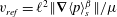 $v_{ref}=\ell ^{2}\Vert \unicode[STIX]{x1D735}\langle p\rangle _{s}^{\unicode[STIX]{x1D6FD}}\Vert /\unicode[STIX]{x1D707}$
, with
$v_{ref}=\ell ^{2}\Vert \unicode[STIX]{x1D735}\langle p\rangle _{s}^{\unicode[STIX]{x1D6FD}}\Vert /\unicode[STIX]{x1D707}$
, with
 $\Vert \unicode[STIX]{x1D735}\langle p\rangle _{s}^{\unicode[STIX]{x1D6FD}}\Vert$
being the maximum value of the pressure gradient over the entire time range of observation of the flow process. In this way, the following boundary conditions can be applied at the edges of the macroscopic domain:
$\Vert \unicode[STIX]{x1D735}\langle p\rangle _{s}^{\unicode[STIX]{x1D6FD}}\Vert$
being the maximum value of the pressure gradient over the entire time range of observation of the flow process. In this way, the following boundary conditions can be applied at the edges of the macroscopic domain:
 $$\begin{eqnarray}\displaystyle & \text{at }x^{\ast }=0,\quad p^{\ast }=nf(t^{\ast }),\quad \forall ~y^{\ast },t^{\ast }>0, & \displaystyle\end{eqnarray}$$
 $$\begin{eqnarray}\displaystyle & \text{at }x^{\ast }=n,\quad p^{\ast }=0,\quad \forall ~y^{\ast },t^{\ast }>0, & \displaystyle\end{eqnarray}$$
with
 $f(t^{\ast })$
being a known function of time that may be applicable to a single unit cell. In addition, periodic conditions at the horizontal boundaries are applied, i.e.
$f(t^{\ast })$
being a known function of time that may be applicable to a single unit cell. In addition, periodic conditions at the horizontal boundaries are applied, i.e.
 $$\begin{eqnarray}\boldsymbol{v}^{\ast }(x^{\ast },0)=\boldsymbol{v}^{\ast }(x^{\ast },1),\quad \forall ~x^{\ast },t^{\ast }>0.\end{eqnarray}$$

Figure 4. Solution domain for the DNS consisting of an array of
 $n$
inline square unit cells of length
$n$
inline square unit cells of length
 $\ell$
.
$\ell$
.
The dimensionless problem was solved for values of
 $t^{\ast }$
ranging from
$t^{\ast }$
ranging from
 $10^{-11}$
up to
$10^{-11}$
up to
 $10$
and, in the rest of this section, results are presented only for a porosity value of 0.4. Similar predictions were obtained for other porosity values. In order to determine the number of unit cells to be considered in the solution domain, so that the results are collected in
$10$
and, in the rest of this section, results are presented only for a porosity value of 0.4. Similar predictions were obtained for other porosity values. In order to determine the number of unit cells to be considered in the solution domain, so that the results are collected in
 ${\mathcal{V}}_{Mh}$
for given flow conditions, a criterion was chosen such that the value of the intrinsic average of the
${\mathcal{V}}_{Mh}$
for given flow conditions, a criterion was chosen such that the value of the intrinsic average of the
 $x$
-component of
$x$
-component of
 $\boldsymbol{v}^{\ast }$
located at the
$\boldsymbol{v}^{\ast }$
located at the
 $(n+1)/2$
unit cell (with
$(n+1)/2$
unit cell (with
 $n$
being an odd number) does not vary by more than
$n$
being an odd number) does not vary by more than
 $10^{-5}\,\%$
when
$10^{-5}\,\%$
when
 $n$
is increased by 2. A value of
$n$
is increased by 2. A value of
 $n=21$
was found appropriate to satisfy this criterion and was hence used as the size of the macroscopic domain in the remainder of the present analysis.
$n=21$
was found appropriate to satisfy this criterion and was hence used as the size of the macroscopic domain in the remainder of the present analysis.
Simulations of the upscaled model were performed in the following manner. Firstly, the initial and dimensionless velocity field (say,
 $\boldsymbol{v}_{0}^{\ast }$
) was determined in a single unit cell from the solution of the steady version of the pore-scale model for a given initial macroscopic pressure gradient (say
$\boldsymbol{v}_{0}^{\ast }$
) was determined in a single unit cell from the solution of the steady version of the pore-scale model for a given initial macroscopic pressure gradient (say
 $\unicode[STIX]{x1D6FB}^{\ast }\langle p_{0}^{\ast }\rangle ^{\unicode[STIX]{x1D6FD}}$
) and Reynolds number
$\unicode[STIX]{x1D6FB}^{\ast }\langle p_{0}^{\ast }\rangle ^{\unicode[STIX]{x1D6FD}}$
) and Reynolds number
 $Re$
. Secondly, the unsteady pore-scale model was solved subject to a desired unsteady macroscopic pressure gradient, keeping
$Re$
. Secondly, the unsteady pore-scale model was solved subject to a desired unsteady macroscopic pressure gradient, keeping
 $Re$
the same. The information from the solution of these two problems was then used to predict the fields of the closure variables
$Re$
the same. The information from the solution of these two problems was then used to predict the fields of the closure variables
 $\unicode[STIX]{x1D63F}$
and
$\unicode[STIX]{x1D63F}$
and
 $\boldsymbol{m}_{0}$
, for the prescribed value of
$\boldsymbol{m}_{0}$
, for the prescribed value of
 $Re$
, from which the effective-medium coefficients,
$Re$
, from which the effective-medium coefficients,
 $\unicode[STIX]{x1D643}_{t}$
and
$\unicode[STIX]{x1D643}_{t}$
and
 $\unicode[STIX]{x1D736}$
, were computed. Once these coefficients are available at all times, they were substituted into the closed upscaled model in order to predict the dynamics of the macroscopic velocity.
$\unicode[STIX]{x1D736}$
, were computed. Once these coefficients are available at all times, they were substituted into the closed upscaled model in order to predict the dynamics of the macroscopic velocity.
Results are organized in case studies as follows: (I) a step change of the pressure gradient from the initial condition to its steady value; (II) a smooth time-decaying flow that leaves the system at rest at steady state; (III) a single pressure gradient pulse; and (IV) an oscillatory flow.
For completeness of the comparison of the different approaches, it is also pertinent to compare the DNS results with the predictions arising from the heuristic model given in (3.22). Note that this model does not require knowledge of the dynamics of the apparent permeability tensor as it only involves its steady value. For all the case studies, the value of
 $H_{xx}^{\ast }$
in the heuristic model was computed with the value of
$H_{xx}^{\ast }$
in the heuristic model was computed with the value of
 $Re$
of interest and the unitary dimensionless pressure gradient along the horizontal
$Re$
of interest and the unitary dimensionless pressure gradient along the horizontal
 $x$
-axis (Lasseux et al.
Reference Lasseux, Abbasian-Arani and Ahmadi2011).
$x$
-axis (Lasseux et al.
Reference Lasseux, Abbasian-Arani and Ahmadi2011).
4.1 Case study I: step change of the pressure gradient
The first two case studies deal with the dynamics from one steady state to another, which is a physical situation that can be of interest in control engineering or in measurements of the dynamic apparent permeability, to cite just a few examples. The goal is to examine the dynamics of the macroscopic velocity and the role played by the initial flow condition. To this end, the first case study will deal with a step change of the pressure gradient. In this way, consider the flow at
 $t^{\ast }\leqslant 0$
to be steady, resulting from a dimensionless pressure gradient value of 0.1. Then suddenly, at
$t^{\ast }\leqslant 0$
to be steady, resulting from a dimensionless pressure gradient value of 0.1. Then suddenly, at
 $t^{\ast }>0$
, let this gradient become unitary, i.e.
$t^{\ast }>0$
, let this gradient become unitary, i.e.
 $$\begin{eqnarray}-\frac{\unicode[STIX]{x2202}\langle p^{\ast }\rangle ^{\unicode[STIX]{x1D6FD}}}{\unicode[STIX]{x2202}x^{\ast }}=\left\{\begin{array}{@{}ll@{}}0.1, & t^{\ast }\leqslant 0,\\ 1.0, & t^{\ast }>0.\end{array}\right.\end{eqnarray}$$

Figure 5. Dynamics of the
 $x$
-component of the macroscale velocity vector, normalized by its steady-state value
$x$
-component of the macroscale velocity vector, normalized by its steady-state value
 $\langle v_{x}^{\ast }\rangle _{ss}^{\unicode[STIX]{x1D6FD}}$
, resulting from the step change on the pressure gradient given in (4.5). In (a), predictions correspond to DNS and the volume averaging method with and without inclusion of the initial flow. In (b), a comparison is shown between predictions from the volume averaging method and the heuristic model. Simulations correspond to a porosity of 0.4 and
$\langle v_{x}^{\ast }\rangle _{ss}^{\unicode[STIX]{x1D6FD}}$
, resulting from the step change on the pressure gradient given in (4.5). In (a), predictions correspond to DNS and the volume averaging method with and without inclusion of the initial flow. In (b), a comparison is shown between predictions from the volume averaging method and the heuristic model. Simulations correspond to a porosity of 0.4 and
 $Re=10^{6}$
.
$Re=10^{6}$
.
In figure 5(a), the response of the system to this forcing is presented in terms of the predicted evolutions of the macroscale velocity obtained from DNS, together with those from the volume averaging method (VAM). Simulations correspond to
 $Re=10^{6}$
and they match those for
$Re=10^{6}$
and they match those for
 $Re=10^{3}$
since results are normalized by the final steady-state value of the velocity (i.e.
$Re=10^{3}$
since results are normalized by the final steady-state value of the velocity (i.e.
 $\langle v_{x}^{\ast }\rangle _{ss}^{\unicode[STIX]{x1D6FD}}$
). This is consistent with the observations made for
$\langle v_{x}^{\ast }\rangle _{ss}^{\unicode[STIX]{x1D6FD}}$
). This is consistent with the observations made for
 $H_{txx}$
presented in the previous section. Clearly, the agreement between DNS and VAM is excellent at all times.
$H_{txx}$
presented in the previous section. Clearly, the agreement between DNS and VAM is excellent at all times.
Note that the steady-state regime is reached at
 $t^{\ast }>0.03$
. In order to have an idea of the time span over which the initial condition plays a relevant role in the macroscale model, predictions are presented for the case in which
$t^{\ast }>0.03$
. In order to have an idea of the time span over which the initial condition plays a relevant role in the macroscale model, predictions are presented for the case in which
 $\boldsymbol{v}_{0}=\mathbf{0}$
(i.e.
$\boldsymbol{v}_{0}=\mathbf{0}$
(i.e.
 $\unicode[STIX]{x1D6FB}^{\ast }\langle p_{0}^{\ast }\rangle ^{\unicode[STIX]{x1D6FD}}=0$
). Under these conditions, closure problem II is completely homogeneous and its solution is zero for all
$\unicode[STIX]{x1D6FB}^{\ast }\langle p_{0}^{\ast }\rangle ^{\unicode[STIX]{x1D6FD}}=0$
). Under these conditions, closure problem II is completely homogeneous and its solution is zero for all
 $\boldsymbol{x}$
(i.e.
$\boldsymbol{x}$
(i.e.
 $\unicode[STIX]{x1D736}=\mathbf{0}$
). In this case, it is noted that the predictions only match those from DNS after
$\unicode[STIX]{x1D736}=\mathbf{0}$
). In this case, it is noted that the predictions only match those from DNS after
 $t^{\ast }>0.01$
, thus illustrating that the initial condition has a significant effect during almost the entire time range in which
$t^{\ast }>0.01$
, thus illustrating that the initial condition has a significant effect during almost the entire time range in which
 $\langle v_{x}^{\ast }\rangle ^{\unicode[STIX]{x1D6FD}}$
is time-dependent. Finally, in figure 5(b), the dynamics of the average velocity resulting from VAM are compared with those obtained from the heuristic model. The latter clearly overpredicts the velocity dynamics in a time range that roughly spans through three orders of magnitude. As expected, the two approaches match at times close to the initial condition and at steady state. This is consistent with the fact that both the heuristic and upscaled models depart from the same initial condition and both converge towards the classical Darcy-like model at sufficiently large time.
$\langle v_{x}^{\ast }\rangle ^{\unicode[STIX]{x1D6FD}}$
is time-dependent. Finally, in figure 5(b), the dynamics of the average velocity resulting from VAM are compared with those obtained from the heuristic model. The latter clearly overpredicts the velocity dynamics in a time range that roughly spans through three orders of magnitude. As expected, the two approaches match at times close to the initial condition and at steady state. This is consistent with the fact that both the heuristic and upscaled models depart from the same initial condition and both converge towards the classical Darcy-like model at sufficiently large time.
4.2 Case study II: time-decaying pressure gradient
As a second case study, consider another change of steady state with two major differences from the previous one: first, let the maximum flow be settled at
 $t^{\ast }\leqslant 0$
, and second, let the macroscopic pressure gradient decay smoothly according to the following expression:
$t^{\ast }\leqslant 0$
, and second, let the macroscopic pressure gradient decay smoothly according to the following expression:
 $$\begin{eqnarray}-\frac{\unicode[STIX]{x2202}\langle p^{\ast }\rangle ^{\unicode[STIX]{x1D6FD}}}{\unicode[STIX]{x2202}x^{\ast }}=\left\{\begin{array}{@{}ll@{}}1-{\displaystyle \frac{t^{\ast }\sin (\unicode[STIX]{x1D714}^{\ast }t^{\ast })}{t_{m}^{\ast }\sin \unicode[STIX]{x1D714}^{\ast }t_{m}^{\ast }}}, & 0\leqslant t^{\ast }\leqslant t_{m}^{\ast },\\ 0, & t^{\ast }>t_{m}^{\ast },\end{array}\right.\end{eqnarray}$$
with
 $t_{m}^{\ast }$
and
$t_{m}^{\ast }$
and
 $\unicode[STIX]{x1D714}^{\ast }$
representing the dimensionless maximum time at which the pressure gradient is non-zero and a given non-dimensional frequency, respectively. The value of
$\unicode[STIX]{x1D714}^{\ast }$
representing the dimensionless maximum time at which the pressure gradient is non-zero and a given non-dimensional frequency, respectively. The value of
 $t_{m}^{\ast }$
was chosen to be smaller than the dimensionless time at which the initial flow was observed to be insensitive in the previous case and was fixed to
$t_{m}^{\ast }$
was chosen to be smaller than the dimensionless time at which the initial flow was observed to be insensitive in the previous case and was fixed to
 $8\times 10^{-4}$
. In order to avoid oscillations, a value of 1000 was chosen for
$8\times 10^{-4}$
. In order to avoid oscillations, a value of 1000 was chosen for
 $\unicode[STIX]{x1D714}^{\ast }$
, yielding the smooth decaying dynamics of the macroscopic pressure gradient shown in figure 6(a). This flow condition may correspond to physical situations in which the pumping device is slowly turned off. Furthermore, for this particular flow condition,
$\unicode[STIX]{x1D714}^{\ast }$
, yielding the smooth decaying dynamics of the macroscopic pressure gradient shown in figure 6(a). This flow condition may correspond to physical situations in which the pumping device is slowly turned off. Furthermore, for this particular flow condition,
 $H_{txx}^{\ast }\rightarrow K_{xx}^{\ast }$
at steady state. This is to be expected because both acceleration and convective inertial effects are no longer present at late times.
$H_{txx}^{\ast }\rightarrow K_{xx}^{\ast }$
at steady state. This is to be expected because both acceleration and convective inertial effects are no longer present at late times.
In figure 6(b), the comparison of the predictions of
 $\langle v_{x}^{\ast }\rangle ^{\unicode[STIX]{x1D6FD}}$
resulting from DNS with those from the upscaled model derived in this work and from the heuristic model for the flow conditions described above is presented. As in the previous case, results are represented after normalization with respect to the maximum value of the velocity, which in this case corresponds to the initial condition. As expected, there is a delay between the time at which the pressure gradient is extinguished and the time at which the average velocity vanishes. In the particular situation examined in figure 6(b), this delay is approximately one order of magnitude in
$\langle v_{x}^{\ast }\rangle ^{\unicode[STIX]{x1D6FD}}$
resulting from DNS with those from the upscaled model derived in this work and from the heuristic model for the flow conditions described above is presented. As in the previous case, results are represented after normalization with respect to the maximum value of the velocity, which in this case corresponds to the initial condition. As expected, there is a delay between the time at which the pressure gradient is extinguished and the time at which the average velocity vanishes. In the particular situation examined in figure 6(b), this delay is approximately one order of magnitude in
 $t^{\ast }$
. Simulations reported in figure 6(b) correspond to a Reynolds-number value of
$t^{\ast }$
. Simulations reported in figure 6(b) correspond to a Reynolds-number value of
 $10^{6}$
and a similar behaviour was obtained for smaller values of
$10^{6}$
and a similar behaviour was obtained for smaller values of
 $Re$
.
$Re$
.

Figure 6. (a) Dynamics of the decaying macroscopic pressure gradient given in (4.6) taking
 $t_{m}^{\ast }=8\times 10^{-4}$
and
$t_{m}^{\ast }=8\times 10^{-4}$
and
 $\unicode[STIX]{x1D714}^{\ast }=1000$
. (b) Dynamics of the
$\unicode[STIX]{x1D714}^{\ast }=1000$
. (b) Dynamics of the
 $x$
-component of the macroscale velocity vector, normalized by its initial value
$x$
-component of the macroscale velocity vector, normalized by its initial value
 $\langle v_{0,x}^{\ast }\rangle ^{\unicode[STIX]{x1D6FD}}$
, resulting from the time-decaying macroscopic pressure gradient. Predictions result from performing DNS, and from the solution of the macroscale model obtained by the volume averaging method and the heuristic model. Simulations correspond to a porosity of 0.4 and
$\langle v_{0,x}^{\ast }\rangle ^{\unicode[STIX]{x1D6FD}}$
, resulting from the time-decaying macroscopic pressure gradient. Predictions result from performing DNS, and from the solution of the macroscale model obtained by the volume averaging method and the heuristic model. Simulations correspond to a porosity of 0.4 and
 $Re=10^{6}$
.
$Re=10^{6}$
.
Once again, predictions from the volume averaging method are in excellent agreement with those from DNS for all values of
 $t^{\ast }$
, while those from the heuristic model only match DNS results in the extreme values of
$t^{\ast }$
, while those from the heuristic model only match DNS results in the extreme values of
 $t^{\ast }$
. Contrary to the previous case, the heuristic model underpredicts the velocity dynamics and this occurs over a time range of roughly three orders of magnitude. Note that, during the early stage of the process, the values of
$t^{\ast }$
. Contrary to the previous case, the heuristic model underpredicts the velocity dynamics and this occurs over a time range of roughly three orders of magnitude. Note that, during the early stage of the process, the values of
 $t^{\ast }$
for which the heuristic model reproduces DNS roughly correspond to those for which the macroscopic pressure gradient is not zero. As a final remark for this case study, it is worth mentioning that the maximum relative per cent error of the predictions from the heuristic model with respect to DNS is approximately 60 %, which is highly contrasting with the one for the predictions of the average model derived here that is below 0.1 %.
$t^{\ast }$
for which the heuristic model reproduces DNS roughly correspond to those for which the macroscopic pressure gradient is not zero. As a final remark for this case study, it is worth mentioning that the maximum relative per cent error of the predictions from the heuristic model with respect to DNS is approximately 60 %, which is highly contrasting with the one for the predictions of the average model derived here that is below 0.1 %.
4.3 Case study III: pressure gradient pulse

Figure 7. Dynamics of the
 $x$
-component of the macroscale velocity as a response to a macroscopic pressure gradient pulse given by (4.7). Results from DNS, and from the solution of the macroscale model obtained by the volume averaging method and the heuristic model correspond to a porosity of 0.4 and (a)
$x$
-component of the macroscale velocity as a response to a macroscopic pressure gradient pulse given by (4.7). Results from DNS, and from the solution of the macroscale model obtained by the volume averaging method and the heuristic model correspond to a porosity of 0.4 and (a)
 $Re=10^{3}$
and (b)
$Re=10^{3}$
and (b)
 $Re=10^{6}$
.
$Re=10^{6}$
.
In the two previous cases, the initial flow has been shown to play quite a significant role for the accuracy of the predictions of the macroscale velocity. The remaining case studies deal with situations for which the fluid was initially at rest in the porous medium, while changes of the macroscopic pressure gradient are operated at
 $t^{\ast }>0$
.
$t^{\ast }>0$
.
In the previous case study, a time delay for the final equilibrium to be reached after the pressure gradient is reduced to zero was highlighted. In the particular case under concern, the interest is to investigate the response to abrupt changes of the macroscopic pressure gradient. Therefore, consider the following dynamics of the macroscopic pressure gradient:
 $$\begin{eqnarray}-\frac{\unicode[STIX]{x2202}\langle p^{\ast }\rangle ^{\unicode[STIX]{x1D6FD}}}{\unicode[STIX]{x2202}x^{\ast }}=\left\{\begin{array}{@{}ll@{}}0, & t^{\ast }\leqslant 0,\\ 1, & 0<t^{\ast }<10^{-2},\\ 0, & t^{\ast }\geqslant 10^{-2}.\end{array}\right.\end{eqnarray}$$
In practice, this corresponds to a pressure gradient given as a finite pulse in the porous medium, which could be of interest, from an experimental point of view, for potential measurements of the dynamic apparent permeability. In figure 7 predictions of the dynamics of the dimensionless macroscale velocity are presented for the two values of the Reynolds number,
 $Re=10^{3}$
(figure 7
a) and
$Re=10^{3}$
(figure 7
a) and
 $Re=10^{6}$
(figure 7
b). Note that the velocity amplitude exhibits a slight decrease as the Reynolds number is increased. In both situations, agreement between DNS and the average model is excellent, whereas the heuristic model overpredicts the velocity for
$Re=10^{6}$
(figure 7
b). Note that the velocity amplitude exhibits a slight decrease as the Reynolds number is increased. In both situations, agreement between DNS and the average model is excellent, whereas the heuristic model overpredicts the velocity for
 $t^{\ast }<10^{-2}$
and underpredicts it for
$t^{\ast }<10^{-2}$
and underpredicts it for
 $t>10^{-2}$
, the largest differences being observed during the first time range. This is consistent with the behaviour observed in the two previous case studies. Indeed, the time period to reach steady state is significantly underpredicted by the heuristic model, compared to DNS or VAM. Finally, it was verified that the results reported in figure 7(a) match those obtained under creeping flow conditions. This is consistent with the fact that, for
$t>10^{-2}$
, the largest differences being observed during the first time range. This is consistent with the behaviour observed in the two previous case studies. Indeed, the time period to reach steady state is significantly underpredicted by the heuristic model, compared to DNS or VAM. Finally, it was verified that the results reported in figure 7(a) match those obtained under creeping flow conditions. This is consistent with the fact that, for
 $\unicode[STIX]{x1D700}=0.4$
,
$\unicode[STIX]{x1D700}=0.4$
,
 $H_{txx}^{\ast }$
is not significantly affected by the Reynolds-number value up to
$H_{txx}^{\ast }$
is not significantly affected by the Reynolds-number value up to
 $Re=10^{4}$
.
$Re=10^{4}$
.
4.4 Case study IV: oscillatory pressure gradient

Figure 8. Dynamics of the
 $x$
-component of the macroscale velocity vector, resulting from a response to an oscillatory change in the macroscopic pressure gradient according to (4.8). Predictions result from performing DNS, from the solution of the macroscale model obtained by the volume averaging method and from the heuristic model. Simulations correspond to a porosity of 0.4 and (a)
$x$
-component of the macroscale velocity vector, resulting from a response to an oscillatory change in the macroscopic pressure gradient according to (4.8). Predictions result from performing DNS, from the solution of the macroscale model obtained by the volume averaging method and from the heuristic model. Simulations correspond to a porosity of 0.4 and (a)
 $Re=10^{3}$
and (b)
$Re=10^{3}$
and (b)
 $Re=10^{6}$
.
$Re=10^{6}$
.
As a final case study, consider the situation in which the fluid saturating the porous medium was initially at rest and then, at
 $t^{\ast }>0$
, it is subjected to a macroscopic pressure gradient that obeys the following expression,
$t^{\ast }>0$
, it is subjected to a macroscopic pressure gradient that obeys the following expression,
 $$\begin{eqnarray}-\frac{\unicode[STIX]{x2202}\langle p^{\ast }\rangle ^{\unicode[STIX]{x1D6FD}}}{\unicode[STIX]{x2202}x^{\ast }}=0.5[1-\cos (\unicode[STIX]{x1D714}^{\ast }t^{\ast })],\end{eqnarray}$$
in which
 $w^{\ast }=1000$
as in case study II. This situation is also interesting because it corresponds to flow in a porous medium induced by, for example, a peristaltic pump or even a ram pump if the experimental conditions allow a permanent oscillatory pressure gradient.
$w^{\ast }=1000$
as in case study II. This situation is also interesting because it corresponds to flow in a porous medium induced by, for example, a peristaltic pump or even a ram pump if the experimental conditions allow a permanent oscillatory pressure gradient.
The resulting predictions of the macroscale velocity are reported in figure 8 following a similar format as the one used in the previous case study. It is observed that the velocity does not exhibit a purely oscillatory dynamics up until
 $t^{\ast }\approx 0.015$
for the two values of
$t^{\ast }\approx 0.015$
for the two values of
 $Re$
considered here (namely
$Re$
considered here (namely
 $Re=10^{3}$
and
$Re=10^{3}$
and
 $10^{6}$
). In the permanent, but time-dependent regime for
$10^{6}$
). In the permanent, but time-dependent regime for
 $\langle v_{x}^{\ast }\rangle ^{\unicode[STIX]{x1D6FD}}$
(i.e. for
$\langle v_{x}^{\ast }\rangle ^{\unicode[STIX]{x1D6FD}}$
(i.e. for
 $t^{\ast }>0.015$
), the heuristic model is not likely to succeed even at late times, since the model is never reduced to a Darcy-like form. This claim is confirmed by the results shown in figure 8. Although the phase is quite well reproduced, the amplitude of the average velocity is significantly overpredicted by the heuristic model. Although results are not presented here for the sake of brevity, it is observed that, for
$t^{\ast }>0.015$
), the heuristic model is not likely to succeed even at late times, since the model is never reduced to a Darcy-like form. This claim is confirmed by the results shown in figure 8. Although the phase is quite well reproduced, the amplitude of the average velocity is significantly overpredicted by the heuristic model. Although results are not presented here for the sake of brevity, it is observed that, for
 $\unicode[STIX]{x1D714}^{\ast }<1000$
, predictions from this model exhibit a much better performance and reproduce the results from DNS in the permanent regime. The conclusion is thus that the heuristic model cannot be considered as a reliable one except in a specific range of frequencies that are likely to depend on the structure of the porous medium and the frequency spectrum. Conversely, the volume averaged model is in excellent agreement with DNS at all frequencies.
$\unicode[STIX]{x1D714}^{\ast }<1000$
, predictions from this model exhibit a much better performance and reproduce the results from DNS in the permanent regime. The conclusion is thus that the heuristic model cannot be considered as a reliable one except in a specific range of frequencies that are likely to depend on the structure of the porous medium and the frequency spectrum. Conversely, the volume averaged model is in excellent agreement with DNS at all frequencies.
As an overview of the case studies in this section, it is worth mentioning that the volume averaged model reproduces the results from DNS whatever the nature of the flow and initial conditions under consideration. This validates the model developed in this work. In these stiff cases, the heuristic model presented poor performance, in general, leading to the conclusion that it is not appropriate.
5 Conclusions
Unsteady flow in porous media is of wide interest for many applications and has been the subject of active work over the past century. However, the available models describing such flows still leave much to be desired, as they are either rather heuristic or remain incomplete, in particular regarding the consideration of inertial effects and, to a lesser extent, the flow initial condition. This motivated the work developed in this article that is dedicated to a formal derivation and analysis of an upscaled model that includes these features for single-phase unsteady flow in rigid and homogeneous periodic porous media. To this end, the pore-scale flow model was upscaled using a short-cut version of the volume averaging method. In this version, the macroscopic forcing was assumed to be spatially invariant in periodic structures. The resulting model expresses the macroscale velocity as a function of two terms: the first one contains the time rate of change of the convolution between a dynamic apparent permeability tensor and the dynamic macroscopic pressure gradient. The second term accounts for the time-decaying influence of the initial velocity. The convolution product holds a memory effect of the flow history. The unsteady upscaled model is clearly in contradiction with the heuristic model, that consists of an ad hoc correction to Darcy’s law by simply including an acceleration term of the average velocity. Moreover, it generalizes a previously reported model that is only applicable under creeping flow conditions (Lions Reference Lions1981; Auriault et al. Reference Auriault, Borne and Chambon1985; Sheng & Zhou Reference Sheng and Zhou1988; Zhou & Sheng Reference Zhou and Sheng1989; Allaire Reference Allaire1992; Mei & Vernescu Reference Mei and Vernescu2010).
Associated with the macroscale model, ancillary closure problems were derived that allow the determination of the dynamics of the effective coefficients. The dynamic apparent permeability tensor,
 $\unicode[STIX]{x1D643}_{t}$
, was shown to be non-symmetric in general. The irreducible decomposition of
$\unicode[STIX]{x1D643}_{t}$
, was shown to be non-symmetric in general. The irreducible decomposition of
 $\unicode[STIX]{x1D643}_{t}$
was achieved, showing that the skew-symmetric part is inherent to inertial effects. This further leads to the conclusion that the dynamic permeability in the creeping regime,
$\unicode[STIX]{x1D643}_{t}$
was achieved, showing that the skew-symmetric part is inherent to inertial effects. This further leads to the conclusion that the dynamic permeability in the creeping regime,
 $\unicode[STIX]{x1D646}_{t}$
, is a symmetric tensor. Positiveness was proved for
$\unicode[STIX]{x1D646}_{t}$
, is a symmetric tensor. Positiveness was proved for
 $\unicode[STIX]{x1D643}_{t}$
in the Laplace domain, proving that
$\unicode[STIX]{x1D643}_{t}$
in the Laplace domain, proving that
 $\overline{\unicode[STIX]{x1D646}}_{t}$
is a symmetric positive definite tensor, although the same is not true for
$\overline{\unicode[STIX]{x1D646}}_{t}$
is a symmetric positive definite tensor, although the same is not true for
 $\overline{\unicode[STIX]{x1D643}}_{t}$
.
$\overline{\unicode[STIX]{x1D643}}_{t}$
.
From the numerical solution of the closure problems, the effective coefficients were predicted in a particular flow situation in simple representations of the porous medium geometry and were found to be functions of time and porosity. After proper normalization, the dependence of the coefficients upon the Reynolds number was collapsed into master curves that were sensitive to variations only in the porosity for the given structure. Although beyond the scope of the present work, further investigations about the extents of this normalization are certainly of interest, as a natural extension to previous works carried out in the creeping regime.
Through a set of stiff flow and initial test conditions, the model was validated by comparison with DNS. In all cases, the agreement between the two approaches was excellent, thus justifying the average model. Conversely, the heuristic model was shown to poorly perform predictions of the macroscale velocity.
As a final point of discussion, it is worth mentioning that the requirement of availability of the velocity fields to solve the closure problems, while not mandatory, does not hinder the value of the macroscale model. The only requirements for the predictions of the effective coefficients are the macroscopic forcing and the initial flow field. In fact, beyond the fundamental interest in this formal model, its relevance lies in the potential use for further upscaling as well as for interpretation of experiments including inertial effects and the influence of the initial condition. Results from this work should serve as a motivation for more theoretical and experimental analyses of unsteady transport phenomena in porous media and many other unsteady processes in hierarchical systems.
Acknowledgements
D.L. would like to gratefully acknowledge the financial support from the French Embassy in Mexico and the IFAL that made possible his stay at UAM (CDMX) in November 2017, a period during which part of this work was completed. In particular, thanks are due to F. Pellegrini, M. Launay and J. J. Vacher. D.L. is also thankful to UAM for its contribution to the cost of his stay. F.J.V.-P. would like to thank the University of Bordeaux and ENSAM for providing invited professor positions during spring 2017 and 2018. The authors are grateful to four anonymous reviewers and to G. Allaire for their constructive remarks.
Appendix A
This appendix is dedicated to a reformulation of the macroscopic momentum equation in the particular situation of creeping flow when the initial condition,
 $\boldsymbol{v}_{0}$
, obeys a Stokes model. It is proved that closure problem I is the only problem that needs to be solved.
$\boldsymbol{v}_{0}$
, obeys a Stokes model. It is proved that closure problem I is the only problem that needs to be solved.
Since in the case under consideration here, the initial flow and the unsteady flow starting at
 $t=0$
, characterized by their velocity and pressure fields (
$t=0$
, characterized by their velocity and pressure fields (
 $\boldsymbol{v}_{0},p_{0}$
) and (
$\boldsymbol{v}_{0},p_{0}$
) and (
 $\boldsymbol{v},p$
), respectively, obey the Stokes model, velocity and pressure fields
$\boldsymbol{v},p$
), respectively, obey the Stokes model, velocity and pressure fields
 $\boldsymbol{u}=\boldsymbol{v}-\boldsymbol{v}_{0}$
and
$\boldsymbol{u}=\boldsymbol{v}-\boldsymbol{v}_{0}$
and
 $P=p-p_{0}$
can be defined satisfying the following unsteady Stokes problem within a periodic unit cell:
$P=p-p_{0}$
can be defined satisfying the following unsteady Stokes problem within a periodic unit cell:
 $$\begin{eqnarray}\displaystyle & \displaystyle \unicode[STIX]{x1D735}\boldsymbol{\cdot }\boldsymbol{u}=0,\quad \text{in }{\mathcal{V}}_{\unicode[STIX]{x1D6FD}},~t>0, & \displaystyle\end{eqnarray}$$
 $$\begin{eqnarray}\displaystyle & \displaystyle \unicode[STIX]{x1D70C}\frac{\unicode[STIX]{x2202}\boldsymbol{u}}{\unicode[STIX]{x2202}t}=-\unicode[STIX]{x1D735}\tilde{P}+\unicode[STIX]{x1D707}\unicode[STIX]{x1D6FB}^{2}\boldsymbol{u}-\unicode[STIX]{x1D735}\langle P\rangle ^{\unicode[STIX]{x1D6FD}}+\unicode[STIX]{x1D70C}(\boldsymbol{b}-\boldsymbol{b}_{0}),\quad \text{in }{\mathcal{V}}_{\unicode[STIX]{x1D6FD}},t>0, & \displaystyle\end{eqnarray}$$
 $$\begin{eqnarray}\displaystyle & \displaystyle \boldsymbol{u}=\mathbf{0},\quad \text{at }{\mathcal{A}}_{\unicode[STIX]{x1D6FD}\unicode[STIX]{x1D70E}},\quad t\geqslant 0, & \displaystyle\end{eqnarray}$$
 $$\begin{eqnarray}\displaystyle & \displaystyle \boldsymbol{u}=\mathbf{0},\quad \text{when }t=0,\quad \text{in }{\mathcal{V}}_{\unicode[STIX]{x1D6FD}}, & \displaystyle\end{eqnarray}$$
 $$\begin{eqnarray}\displaystyle & \displaystyle \langle \tilde{P}\rangle ^{\unicode[STIX]{x1D6FD}}=0,\quad t>0, & \displaystyle\end{eqnarray}$$
 $$\begin{eqnarray}\displaystyle & \displaystyle \boldsymbol{u}(\boldsymbol{r}+\boldsymbol{l}_{i})=\boldsymbol{u}(\boldsymbol{r}),\quad \tilde{P}(\boldsymbol{r}+\boldsymbol{l}_{i})=\tilde{P}(\boldsymbol{r}),\quad t>0,\quad i=1,2,3, & \displaystyle\end{eqnarray}$$
 $\tilde{P}=\tilde{p}-\tilde{p}_{0}$
and
$\tilde{P}=\tilde{p}-\tilde{p}_{0}$
and
 $\boldsymbol{b}_{0}=\boldsymbol{b}(t=0)$
.
$\boldsymbol{b}_{0}=\boldsymbol{b}(t=0)$
. Since the initial condition for the problem for
 $\boldsymbol{u}$
and
$\boldsymbol{u}$
and
 $P$
is zero, the associated macroscopic momentum equation can be written as (see (3.21))
$P$
is zero, the associated macroscopic momentum equation can be written as (see (3.21))
 $$\begin{eqnarray}\langle \boldsymbol{u}\rangle =-\frac{1}{\unicode[STIX]{x1D707}}\frac{\unicode[STIX]{x2202}\unicode[STIX]{x1D646}_{t}}{\unicode[STIX]{x2202}t}\,\ast \boldsymbol{\cdot }\,(\unicode[STIX]{x1D735}\langle P\rangle ^{\unicode[STIX]{x1D6FD}}-\unicode[STIX]{x1D70C}(\boldsymbol{b}-\boldsymbol{b}_{0})),\quad t>0,\end{eqnarray}$$
where
 $\unicode[STIX]{x1D646}_{t}$
is the dynamic permeability in the absence of inertia. In addition, at the macroscale, the initial steady flow obeys a Darcy-like equation, i.e.
$\unicode[STIX]{x1D646}_{t}$
is the dynamic permeability in the absence of inertia. In addition, at the macroscale, the initial steady flow obeys a Darcy-like equation, i.e.
 $$\begin{eqnarray}\displaystyle \langle \boldsymbol{v}_{0}\rangle =-\frac{\unicode[STIX]{x1D646}}{\unicode[STIX]{x1D707}}\boldsymbol{\cdot }(\unicode[STIX]{x1D735}\langle p_{0}\rangle ^{\unicode[STIX]{x1D6FD}}-\unicode[STIX]{x1D70C}\boldsymbol{b}_{0}),\quad t=0, & & \displaystyle\end{eqnarray}$$
where
 $\unicode[STIX]{x1D646}$
is the intrinsic permeability of the medium corresponding to
$\unicode[STIX]{x1D646}$
is the intrinsic permeability of the medium corresponding to
 $\unicode[STIX]{x1D646}_{t}$
at sufficiently large times. When
$\unicode[STIX]{x1D646}_{t}$
at sufficiently large times. When
 $\boldsymbol{u}$
and
$\boldsymbol{u}$
and
 $P$
are replaced by their expressions in terms of
$P$
are replaced by their expressions in terms of
 $\boldsymbol{v}$
,
$\boldsymbol{v}$
,
 $\boldsymbol{v}_{0}$
,
$\boldsymbol{v}_{0}$
,
 $p$
and
$p$
and
 $p_{0}$
in (A 2), the unsteady macroscopic form of the momentum equation in the case under study is given by
$p_{0}$
in (A 2), the unsteady macroscopic form of the momentum equation in the case under study is given by
 $$\begin{eqnarray}\displaystyle \langle \boldsymbol{v}\rangle =-\frac{1}{\unicode[STIX]{x1D707}}\frac{\unicode[STIX]{x2202}\unicode[STIX]{x1D646}_{t}}{\unicode[STIX]{x2202}t}\,\ast \boldsymbol{\cdot }\,(\unicode[STIX]{x1D735}\langle p\rangle ^{\unicode[STIX]{x1D6FD}}-\unicode[STIX]{x1D70C}\boldsymbol{b})-\frac{1}{\unicode[STIX]{x1D707}}(\unicode[STIX]{x1D646}-\unicode[STIX]{x1D646}_{t})\boldsymbol{\cdot }(\unicode[STIX]{x1D735}\langle p_{0}\rangle ^{\unicode[STIX]{x1D6FD}}-\unicode[STIX]{x1D70C}\boldsymbol{b}_{0}),\quad t>0 & & \displaystyle\end{eqnarray}$$
or, equivalently,
 $$\begin{eqnarray}\displaystyle \langle \boldsymbol{v}\rangle & = & \displaystyle -\frac{1}{\unicode[STIX]{x1D707}}\frac{\unicode[STIX]{x2202}\unicode[STIX]{x1D646}_{t}}{\unicode[STIX]{x2202}t}\,\ast \boldsymbol{\cdot }\,(\unicode[STIX]{x1D735}\langle p\rangle ^{\unicode[STIX]{x1D6FD}}-\unicode[STIX]{x1D70C}\boldsymbol{b})+(\unicode[STIX]{x1D644}-\unicode[STIX]{x1D646}_{t}\boldsymbol{\cdot }\unicode[STIX]{x1D646}^{-1})\boldsymbol{\cdot }\langle \boldsymbol{v}_{0}\rangle ,\quad t>0.\end{eqnarray}$$
This clearly shows that, in this particular case, the only closure problem that needs to be solved is problem I, yielding
 $\unicode[STIX]{x1D646}_{t}$
(and
$\unicode[STIX]{x1D646}_{t}$
(and
 $\unicode[STIX]{x1D646}$
at sufficiently long time).
$\unicode[STIX]{x1D646}$
at sufficiently long time).


