


1. Introduction
A feedback control method for skin-friction drag reduction by Choi, Moin & Kim (Reference Choi, Moin and Kim1994), called opposition control, is a physics-based control strategy that mitigates the strength of near-wall streamwise vortices in a channel by providing blowing and suction at the wall  $(\phi )$ which is 180
 $^{\circ }$ out-of-phase with the instantaneous wall-normal velocity
  $v$ above the wall. Choi et al. (Reference Choi, Moin and Kim1994) showed that the sensing-plane location of
  $y^+ \approx 10$ (i.e.
  $\phi =-v_{y^+\approx 10}$) was the optimal location providing 25 % skin-friction drag reduction in a turbulent channel flow, where
  $y^+=yu_{\tau }/\nu$,
  $y$ is the wall-normal distance from the wall,
  $u_{\tau }$ is the wall shear velocity and
  $\nu$ is the kinematic viscosity. Later, a number of studies have investigated the detailed characteristics of opposition control. Hammond, Bewley & Moin (Reference Hammond, Bewley and Moin1998) showed that the sensing-plane location of
  $y^+ = 15$ provided slightly more drag reduction than that of
  $y^+ = 10$. Chung & Talha (Reference Chung and Talha2011) reported that the maximum drag-reduction rate with a given sensing location depended on the amplitude of blowing/suction. For example, approximately 10 % drag reduction was obtained with
  $\phi =-(v_{y^+=25}/5)$, whereas the drag increased with
  $\phi =-v_{y^+=25}$. The effect of the Reynolds number had been also investigated; the maximum drag-reduction rate decreased as the Reynolds number increased (Chang, Collis & Ramakrishnan Reference Chang, Collis and Ramakrishnan2002; Iwamoto, Suzuki & Kasagi Reference Iwamoto, suzuki and Kasagi2002), but drag reduction of 20 % was still achieved at
  $Re_{\tau } = 1000$ with a sensing location of
  $y^+ = 13.5$ (Wang, Huang & Xu Reference Wang, Huang and Xu2016), where
  $Re_{\tau } = u_{\tau } \delta / \nu$ and
  $\delta$ is the channel half-height. Rebbeck & Choi (Reference Rebbeck and Choi2001, Reference Rebbeck and Choi2006) experimentally conducted opposition control with a single pair of sensing probe and actuator, and showed that strong downwash motions near the wall were suppressed by the blowing at the wall.
Since it is difficult and even impractical to measure the instantaneous wall-normal velocity  $v$ at
  $y^+=10$ (
 $v_{10}$ hereafter), opposition controls using predicted
  $v_{10}$'s (
 $v_{10}^{pred}$'s) from wall variables such as the wall pressure and shear stresses have been searched for. For example, Choi et al. (Reference Choi, Moin and Kim1994) conducted a Taylor series expansion on near-wall wall-normal velocity,
 \begin{equation} v(y) = \frac{1}{2} y^2 \left. \frac{\partial^2 v}{\partial y^2}\right|_w + \cdots, \end{equation}
where  $y=0$ is the wall location and the subscript
  $w$ denotes the wall. Due to the continuity
  $({\partial v}/{\partial y} = - {\partial u}/{\partial x} - {\partial w}/{\partial z})$,
 \begin{equation} v(y) = -\frac{1}{2}{y^2} \left[\frac{\partial }{\partial x}{\left. \frac{\partial u}{\partial y} \right|_w}+ \frac{\partial }{\partial z}{\left.\frac{\partial w}{\partial y} \right|_w}\right] +\cdots, \end{equation}
where  $x$ and
  $z$ are the streamwise and spanwise directions, respectively, and
  $u$ and
  $w$ are the corresponding velocity components. Because the first term in the bracket had a negligible correlation with v 10,
 \begin{equation} v(y) \approx -\frac{1}{2} y^2 \frac{\partial}{\partial z} \left. \frac{\partial w}{\partial y} \right|_w, \end{equation}
and they applied
 \begin{equation} \left. \phi = v_{10, rms} \frac{\partial}{\partial z}\left. \frac{\partial w}{\partial y} \right|_w \right/ \left(\frac{\partial}{\partial z}\left. \frac{\partial w}{\partial y} \right|_w\right)_{rms}, \end{equation}
resulting in approximately 6 % drag reduction. The correlation coefficient between  $v_{10}$ and
  $v$ predicted using this Taylor series expansion was
  $\rho _{v_{10}} \approx 0.75$, which is not low but not high enough to produce a significant amount of drag reduction. Here, the correlation coefficient between
  $v_{10}$ and
  $\psi$ is defined as
  $\rho _{v_{10}} = \langle v_{10}(x,z,t) \psi (x,z,t) \rangle /({v_{10,rms}}{\psi _{rms}})$, where
  $\langle \ \rangle$ denotes the averaging in the homogeneous directions (
 $x, z$) and time, and the subscript
  $rms$ indicates the root-mean square. Bewley & Protas (Reference Bewley and Protas2004) retained even high-order terms (up to the terms of
  $O(y^5)$) in the Taylor series expansion, but high-order terms rather degraded the correlation. Several studies have presented methods of predicting the near-wall velocity from the flow variables at the wall or away from the wall using direct numerical simulation (DNS) data. Podvin & Lumley (Reference Podvin and Lumley1998) conducted a proper orthogonal decomposition (POD) to the streamwise and spanwise wall velocity gradients (
 $\partial u/\partial y \vert _w$ and
  $\partial w/\partial y \vert _w$), and showed that near-wall streamwise streaks were reconstructed well but wall-normal and spanwise velocities were not very well reproduced. Bewley & Protas (Reference Bewley and Protas2004) developed an adjoint-based estimator which was optimized by solving the adjoint Navier–Stokes equations. An estimator using all three wall variables (
 $\partial u/\partial y \vert _w$,
  $\partial w/\partial y \vert _w$ and
  $p_w$ (wall pressure)) showed a better prediction of near-wall velocity components for a turbulent channel flow at
  $Re_{\tau }=100$ than that from the Taylor series expansion, showing
  $\rho _{v_{10}} \approx 0.88$. Hœpffner et al. (Reference Hœpffner, Chevalier, Bewley and Henningson2005) and Chevalier et al. (Reference Chevalier, Hœpffner, Bewley and Henningson2006) developed a linear estimation model based on the linearized Navier–Stokes equations and a Kalman filter. They improved the performance of the estimator by treating nonlinear terms in the Navier–Stokes equations as the external forcings which were sampled from DNS data, and obtained
  $\rho _{v_{10}} \approx 0.85$ using three wall variables of
  $\omega _y \vert _w$,
  $\partial ^2 v/\partial y^2 \vert _w$, and
  $p_w$ for a turbulent channel flow at
  $Re_{\tau }=100$, where
  $\omega _y \vert _w$ is the wall-normal vorticity at the wall. Illingworth, Monty & Marusic (Reference Illingworth, Monty and Marusic2018) applied a linear estimator similar to that of Chevalier et al. (Reference Chevalier, Hœpffner, Bewley and Henningson2006) to a turbulent channel flow at
  $Re_{\tau }=1000$, and predicted large scale
  $u$ at an arbitrary
  $y$ location using all three velocity components at
  $y^+=197$. A linear estimator based on
  $\partial u/\partial y \vert _w$ also reasonably predicted large scale
  $u$ at an arbitrary
  $y$, but its performance was not better than that using all three velocity components at
  $y^+=400$ in a turbulent channel flow at
  $Re_{\tau }=2000$ (Oehler, Garcia-Gutiérrez & Illingworth Reference Oehler, Garcia-Gutiérrez and Illingworth2018). Oehler & Illingworth (Reference Oehler, Illingworth, Lau and Kelso2018) used an estimator to impose a body forcing
  $f_b \vert _{y=y_b}$ predicted by sensing
  $u \vert _{y=y_s}$ or
  $\partial u/\partial y \vert _w$, for the minimization of the magnitude of the velocity fluctuations in a turbulent channel flow at
  $Re_{\tau }=2000$, and obtained a minimum value when
  $y_s=0.26 \delta$ and
  $y_b = 0.29 \delta$.
Another approach for predicting  $v_{10}$ with the wall variables is using a neural network. Lee et al. (Reference Lee, Kim, Babcock and Goodman1997) applied a neural network for the first time to perform a control with
  $v_{10}^{pred}$ (predicted
  $v_{10}$) in a turbulent channel flow at
  $Re_{\tau }=100$. They used the information of
  $\partial w/\partial y \vert _w$ along the spanwise direction to predict
  $v_{10}$ (i.e.
  $v_{10}^{pred}(x,z)=f({\left . \partial w/\partial y\right |_w}(x,z\pm n\Delta z)),\ n=0,1,2,\ldots )$, and showed that the spanwise length of at least 90 wall units was required for accurately predicting
  $v_{10}$ with
  $\partial w/\partial y \vert _w$'s, resulting in
  $\rho _{v_{10}}$ of approximately 0.85 and 18 % drag reduction. Lorang, Podvin & Le Quéré (Reference Lorang, Podvin and Le Quéré2008) obtained the first POD mode of
  $v_{10}$ with a neural network by sensing whole domain information of
  $\partial w/\partial y \vert _w$ in a turbulent channel flow at
  $Re_{\tau }=140$, and performed a control with it, resulting in a drag reduction of 13 % which was slightly smaller than the amount of drag reduction (14 %) with the method of Lee et al. (Reference Lee, Kim, Babcock and Goodman1997). The difference in the amounts of drag reduction from those two studies may come from the difference in the Reynolds numbers, i.e.
  $Re_{\tau }=100$ versus
  $140$. Milano & Koumoutsakos (Reference Milano and Koumoutsakos2002) used a neural network to predict high-order terms (
 $O(y^3)$) of the Taylor series expansion of near-wall velocity components by sensing
  $p_w$,
  $\partial u/\partial y \vert _w$ and
  $\partial w/\partial y \vert _w$, and the reconstructed streamwise and spanwise velocities had correlations higher than 0.9, but
  $\rho _{v_{10}}$ (obtained from the continuity) was only approximately 0.6. Recently, Yun & Lee (Reference Yun and Lee2017) used
  $p_w$ to predict
  $v_{10}$ by a neural network with the streamwise and spanwise sensing lengths of 90 and 45 wall units, respectively, and showed
  $\rho _{v_{10}}=0.85$. These previous studies showed that the neural network is an attractive tool to predict
  $v_{10}$ with wall-variable sensing, but shallow neural networks (one nonlinear layer in Lee et al. (Reference Lee, Kim, Babcock and Goodman1997) and Lorang et al. (Reference Lorang, Podvin and Le Quéré2008), two nonlinear layers in Milano & Koumoutsakos (Reference Milano and Koumoutsakos2002) and Yun & Lee (Reference Yun and Lee2017)) may not be sufficient to yield a high
  $\rho _{v_{10}}$.
In recent years, machine learning, especially deep learning (LeCun, Bengio & Hinton Reference LeCun, Bengio and Hinton2015), has shown remarkable performance. Güemes, Discetti & Ianiro (Reference Güemes, Discetti and Ianiro2019) applied an extended POD and convolutional neural networks, respectively, to reconstruct large- and very large-scale motions in a turbulent channel flow based on the wall shear stress measurement, and showed that the convolutional neural networks performed significantly better than the extended POD. Kim & Lee (Reference Kim and Lee2020) used a nine-layer convolutional neural network (CNN) to predict the heat flux at the wall using wall variables ( $p_w$,
  $\partial u/\partial y \vert _w$ and
  $\partial w/\partial y \vert _w$), and showed that the CNN outperformed a linear regression. So far, there is no attempt to apply a CNN to the prediction of the near-wall flow (
 $v_{10}$) from the flow variables at the wall and to the flow control in a feedback manner. Therefore, in the present study we first aim at predicting
  $v_{10}$ using a CNN which is currently the most successful deep learning method in discovering spatial distributions of a raw input that are closely related to a desired output, where the wall flow variables (
 $p_w$,
  $\partial u/\partial y \vert _w$ and
  $\partial w/\partial y \vert _w$) and
  $v_{10}$ are the input and output, respectively, used in this study. We investigate how high
  $\rho _{v_{10}}$ can be achieved from the CNN as compared to fully connected neural networks (FCNN) used in the previous studies (Lee et al. Reference Lee, Kim, Babcock and Goodman1997; Milano & Koumoutsakos Reference Milano and Koumoutsakos2002; Lorang et al. Reference Lorang, Podvin and Le Quéré2008; Yun & Lee Reference Yun and Lee2017). We then perform opposition control with
  $v_{10}^{pred}$ predicted by the CNN. Because the controlled flow is not available in practice, we train our CNN only with the uncontrolled flow. Note that previous studies (Lee et al. Reference Lee, Kim, Babcock and Goodman1997; Lorang et al. Reference Lorang, Podvin and Le Quéré2008) used controlled flows to train the neural network. Finally, we apply the CNN to a higher Reynolds number flow to see if the prediction and control capabilities are maintained even if the CNN is trained with a lower Reynolds number flow. Details of the problem setting, CNN, and numerical method are presented in § 2. The prediction performance of the CNN is given in § 3. In § 4 we provide the results of control with
  $v_{10}^{pred}$ from the CNN. An application to a higher Reynolds number flow is given in § 5, followed by conclusions. In the appendices the results from other machine learning techniques such as the random forest and FCNN are given and their results are briefly discussed.
2. Methodology
2.1. Problem setting
In the present study we predict  $v_{10}$ from a spatial distribution of wall variables (
 $\chi _w$) in a turbulent channel flow, where a CNN is used to extract hidden features of
  $\chi _w$ which may closely represent
  $v_{10}$. We consider three different wall variables (
 $\chi _w=p_w$,
  $\partial u/\partial y \vert _w$ and
  $\partial w/\partial y \vert _w$) that are measurable quantities in real systems (Kasagi, Suzuki & Fukagata Reference Kasagi, Suzuki and Fukagata2008). Each of these wall variables is used to predict
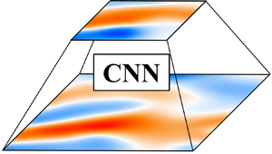
  $v_{10}$ (figure 1) and is used for the control. Since Bewley & Protas (Reference Bewley and Protas2004) and Chevalier et al. (Reference Chevalier, Hœpffner, Bewley and Henningson2006) showed that using more wall variables improved the prediction performance, all three wall variables are also used to predict
  $v_{10}$ and the results are given in § 4.3. A region on the wall (coloured in yellow) in figure 1 is an example of the sensing region of the wall variable
  $\chi _w$ whose streamwise and spanwise lengths are approximately 90 wall units. The size of each sensing region is selected considering those of previous studies in which at least 90 wall units in the spanwise direction was required for
  $\partial w/\partial y \vert _w$ (Lee et al. Reference Lee, Kim, Babcock and Goodman1997), and 90 wall units in the streamwise direction was sufficient for
  $p_w$ (Yun & Lee Reference Yun and Lee2017). One of the wall variables is the input of the present CNN (see below), and the output is
  $v_{10}^{pred}$ at the centre location of each sensing region. As we show below, this size is not big enough to include the influence of
  $v_{10}$ on the wall variables, but is still sufficient to have a high correlation between
  $v_{10}$ and
  $v_{10}^{pred}$.

Figure 1. Schematic diagram on the relation between the predicted  $v$ at
  $y^+=10$ (
 $v_{10}^{pred}$) and wall-variable distribution with a CNN in a turbulent channel flow. The input (
 $\chi _w$) of the CNN is one of
  $p_w$,
  $\partial u/\partial y \vert _w$ and
  $\partial w/\partial y \vert _w$, and the output is
  $v_{10}^{pred}$.
The two-point correlation coefficient  $\rho$ between
  $v_{10}$ and
  $\chi _w$ in a turbulent channel flow is defined as
 \begin{equation} \rho \left(\Delta x, \Delta z \right)=\frac{\langle v_{10} (x,z,t)\chi_w (x+\Delta x, z+ \Delta z,t) \rangle} {v_{10,rms}\chi_{w,rms}}, \end{equation}
where  $\langle v_{10} \rangle =0$, and
  $\Delta x$ and
  $\Delta z$ are the separation distances in the streamwise and spanwise directions, respectively. Figure 2 shows the contours of the two-point correlations for three different flows: (
 $a$–
$a$– $c$) uncontrolled flow at
  $Re_{\tau } = 178$, (
 $d$–
$d$– $f$) controlled flow with opposition control (Choi et al. Reference Choi, Moin and Kim1994) at
  $Re_{\tau } = 178$, and (
 $g$–
$g$– $i$) uncontrolled flow at
  $Re_{\tau } = 578$, where
  $Re_{\tau } = u_{\tau _o} \delta / \nu$ and
  $u_{\tau _o}$ is the wall shear velocity of the uncontrolled flow. These correlation contours indicate that there are distinct regions of close relations between
  $v_{10}$ and
  $\chi _w$. For the uncontrolled flow at
  $Re_{\tau } = 178$ (figure 2
 $a$–
$a$– $c$), the wall pressure has the highest correlation on the downstream of
  $v_{10}$, but has the lowest maximum correlation among three wall variables investigated in this study. The streamwise wall shear rate
  $\partial u/\partial y \vert _w$ has the highest correlation at the upstream of
  $v_{10}$, whereas the correlation with the spanwise wall shear rate
  $\partial w/\partial y \vert _w$ is highest at slightly downstream but sideways locations. The two-point correlation is highest for the spanwise wall shear rate, but this correlation magnitude (
 $\rho = 0.56$) is not high enough to accurately predict
  $v_{10}$. Also, these correlation contours themselves do not provide how one can construct
  $v_{10}$ from this information. Hence, in the present study, we construct
  $v_{10}$ from the wall-variable information in
  $-45 < \Delta x^+ < 45$ and
  $-45 < \Delta z^+ < 45$ using a CNN, and discuss how high correlations can be obtained from this approach.

Figure 2. Contours of the correlation coefficients between  $v_{10}$ and
  $\chi _w$: (
 $a$–
$a$– $c$) uncontrolled flow at
  $Re_{\tau } = 178$; (
 $d$–
$d$– $f$) controlled flow at
  $Re_{\tau } = 178$ by opposition control; (
 $g$–
$g$– $i$) uncontrolled flow at
  $Re_{\tau } = 578$. (
 $a{,}d{,}g$)
  $\chi _w = p_w$, (
 $b{,}e{,}h$)
  $\chi _w = \partial u /\partial y \vert _w$ and (
 $c{,}f{,}i$)
  $\chi _w = \partial w / \partial y \vert _w$. Solid circles at the centre denote the location of
  $v_{10}$ (
 $\Delta x = \Delta z = 0$), and cross symbols are the locations of the maximum correlation magnitude. The values of
  $\rho$ at these locations are given at the bottom of each figure. Here,
  $\Delta x^+ = \Delta x u_{\tau _o}/\nu$ and
  $\Delta z^+ = \Delta z u_{\tau _o}/\nu$.
For the controlled flow at  $Re_{\tau } = 178$ (figure 2
 $d$–
$d$– $f$), the correlations with
  $p_w$ and
  $\partial w/\partial y \vert _w$ are very similar to those for the uncontrolled flow. This suggests that a CNN trained with the uncontrolled flow can be applied to predict
  $v_{10}$ for the controlled flow and also to control the flow in a feedback manner even without requiring training data of the controlled flow. On the other hand, the correlations with
  $\partial u/\partial y \vert _w$ have opposite signs in many places to those for the uncontrolled flow. This is because the blowing and suction at the wall from opposition control changes
  $\partial u/\partial y \vert _w$ to be approximately
  $180^{\circ }$ out-of-phase different from
  $v_{10}$. For the uncontrolled flow at
  $Re_{\tau } = 578$ (figure 2
 $g$–
$g$– $i$), the correlations are very similar to those at
  $Re_{\tau } = 178$, as the near-wall flow is well scaled in wall units, which suggests that the CNN trained at a lower Reynolds number should be applicable to the flow at a higher Reynolds number.
Note that near-wall flow structures are significantly changed by opposition control (Choi et al. Reference Choi, Moin and Kim1994; Hammond et al. Reference Hammond, Bewley and Moin1998), and a higher Reynolds number flow contains smaller scales than those at  $Re_{\tau } = 178$. Therefore, the success of the present control based on a CNN trained with uncontrolled flow at
  $Re_{\tau } = 178$ relies on the proper selection of wall sensing variable that maintains a similar correlation coefficient with
  $v_{10}$ for controlled and higher Reynolds number flows. For the present turbulent channel flow, the wall sensing variables satisfying this requirement are
  $p_w$ and
  $\partial w/\partial y \vert _w$, but
  $\partial u/\partial y \vert _w$ fails to satisfy this requirement. The details of the CNN used are provided in § 2.3. Other machine learning techniques such as the Lasso, random forest and FCNN are also tested, and comparisons of the prediction performance by different machine learning techniques are given in appendix A.
2.2. The dataset
The dataset ( $v_{10}^{true}$,
  $\chi _w$) for training a CNN is obtained from direct numerical simulation of a turbulent channel flow at
  $Re_{\tau } = 178$, where
  $v_{10}^{true}= v_{10}$. The governing equations for the continuity and incompressible Navier–Stokes equations are
 \begin{gather} \frac{\partial {{u}_{i}}}{\partial {{x}_{i}}}=0, \end{gather}
 \begin{gather} \frac{\partial {u_i}}{\partial t}+\frac{\partial {u_i}{u_j}}{\partial {x_j}}=-\frac{\textrm{d}P}{\textrm{d}{x_1}}{{\delta }_{1i}}-\frac{\partial p}{\partial {x_i}}+\frac{1}{Re}\frac{{{\partial }^{2}}{u_i}}{\partial {x_j}\partial {x_j}}, \end{gather}
where  $x_i\, (= (x,y,z))$ are the Cartesian coordinates,
  $u_i\, (= (u,v,w))$ are the corresponding velocity components,
  $p$ is the pressure fluctuation,
  $-\textrm {d}P/\textrm {d}x_1$ is the mean pressure gradient to maintain a constant mass flow rate in a channel. The Reynolds number is
  $Re= 5600$ based on the bulk velocity (
 $u_b$) and channel height (
 $2 \delta$), and is 178 based on the wall shear velocity of the uncontrolled flow (
 $u_{\tau _o}$) and channel half-height (
 $\delta$). A semi-implicit fractional step method is used to solve (2.2) and (2.3), where a third-order Runge–Kutta and the Crank–Nicolson schemes are used for the convection and diffusion terms, respectively. For spatial derivatives, the second-order central difference scheme is used. The no-slip condition is applied to the upper and lower walls, and periodic boundary conditions are used in the wall-parallel directions. The computational domain size is
  $3{\rm \pi} \delta (x) \times 2\delta (y) \times {\rm \pi}\delta (z)$ and the number of grid points is
  $192(x) \times 129(y) \times 128(z)$. In the wall-normal direction a non-uniform grid is used with
  ${\Delta }{y^+} \approx 0.2 - 7.0$ (dense grids near the wall). Uniform grids are used in the wall-parallel directions with
  ${\Delta }{x^+} \approx 8.7$ and
  ${\Delta }{z^+} \approx 4.4$.
The simulation starts with a laminar velocity profile with random perturbations and continues until the flow reaches a fully developed state. Then, 740 instantaneous fields of  $v_{10}^{true}$ and
  $\chi _w$'s (
 $=p_w$,
  $\partial u/\partial y \vert _w$, and
  $\partial w/\partial y \vert _w$) are stored during
  $T^+=Tu_{\tau _o}^2/\nu =29\,560$ with an interval of
  ${\Delta }T^+=40$, where
  $v_{10}^{true}$ is the label for output of a CNN (
 $v_{10}^{pred}$), and
  $\chi _w$'s are the input whose domain size is approximately
  $90 (l_x^+) \times 90 (l_z^+)$ in wall units (corresponding to
  $11 \times 21$ grid points, respectively), as shown in figure 1. Here, one instantaneous field contains the information of
  $\chi _w$'s and
  $v_{10}^{true}$ at both sides of the channel. The
  $\chi _w$ and
  $v_{10}^{true}$ are normalized with their root-mean-square (subscript
  $rms$) values as
 \begin{equation} \chi_w^{\ast} =\frac{\chi_w - \langle \chi_w \rangle}{\chi_{w, rms}}, \quad v_{10}^{\ast} =\frac{v_{10}^{true}}{v_{10, rms}^{true}}, \end{equation}
where  $\langle \chi _w \rangle$ denotes the mean value of
  $\chi _w$. The dataset of
  $\chi _w^{\ast }$ and
  $v_{10}^{\ast }$ is divided into three sets of different sizes, i.e. training, validation and test sets. Only the training set is used for optimizing a CNN. The validation set is used for checking the optimization process at each training iteration, and the prediction performance is evaluated with the test set after the whole training procedure is finished. We use 700 instantaneous fields (containing 34 406 400 pairs of
  $\chi _w$'s and
  $v_{10}^{true}$) for the training, and extract data at every third grid point in the streamwise and spanwise directions (resulting in approximately 3.8 million pairs of
  $\chi _w$'s and
  $v_{10}^{true}$), respectively, to exclude highly correlated data. Twenty instantaneous fields (containing 983,040 pairs of
  $\chi _w$'s and
  $v_{10}^{true}$) are used for each validation and test set. Here, we use the number of training data of
  $N_{train} \approx 3.8 \times 10^6$ which is approximately three times that used in the ImageNet large-scale visual recognition challenge (ILSVRC) for developing convolutional neural networks (Krizhevsky, Sutskever & Hinton Reference Krizhevsky, Sutskever, Hinton, Pereira, Burges and Bottou2012; Simonyan & Zisserman Reference Simonyan and Zisserman2014; Szegedy et al. Reference Szegedy, Liu, Jia, Sermanet, Reed, Anguelov, Erhan, Vanhoucke and Rabinovich2014; He et al. Reference He, Zhang, Ren and Sun2015; Russakovsky et al. Reference Russakovsky, Deng, Su, Krause, Satheesh, Ma, Huang, Karpathy, Khosla and Bernstein2015). This is because the present training searches for the spatial correlations of
  $\chi _w$'s and
  $v_{10}^{true}$ and, thus, it possesses some similarity with that of image recognition in the ILSVRC, but it may require more training data due to the unsteady characteristics of the present problem than that used in the ILSVRC. In appendix B we show that
  $N_{train} \approx 3.8 \times 10^6$ is sufficient for the present problem.
2.3. Convolutional neural network
The CNN is a class of neural network, composed of input, hidden and output layers with artificial neurones. The CNN uses a discrete convolution operation with filters to construct the next layer keeping spatially two-dimensional feature maps. Therefore, unlike a FCNN whose inputs to a neurone are outputs from all neurones in the previous layer, local outputs from the previous layer in the CNN are inputs to a neurone, and neurones share the same weights (LeCun et al. Reference LeCun, Boser, Denker, Henderson, Howard, Hubbard, Jackel and Touretzky1989, Reference LeCun, Bengio and Hinton2015). Figure 3 shows the architecture of the CNN used in the present study. We use 17 hidden layers, one average pooling layer and one linear layer adopting a residual block proposed by He et al. (Reference He, Zhang, Ren and Sun2015). For the hidden layers without downsampling, we use a filter size of  $3\times 3$ or
  $5\times 5$, with a stride of 1 for the convolution, where the stride is the magnitude of movement between applications of the filter to the input feature map (Singh & Manure Reference Singh and Manure2019). After the first and second downsampling layers, the height (
 $h_m$) and width (
 $w_m$) of the feature maps are reduced by half, and the depth (
 $d_m$) is doubled, as in He et al. (Reference He, Zhang, Ren and Sun2015). We use a convolution operation with a stride of 2 and a filter size of
  $2\times 2$ for the first and second downsampling layers. After
  $h_m$ or
  $w_m$ of the feature map becomes equal to
  $h_f$ or
  $w_f$ of the filter, respectively, we use global average pooling for the last downsampling (average pooling layer in figure 3), where the feature map is averaged while keeping the depth unchanged. After the average pooling layer, the feature map is connected to the linear layer to print out
  $v_{10}^{pred}$ without an activation function. In the present CNN Relu (Nair & Hinton Reference Nair, Hinton, Fürnkranz and Joachims2010) is used as the activation function, and a batch normalization (Ioffe & Szegedy Reference Ioffe and Szegedy2015) is applied after each convolution operation. All weights (
 $w_j$) in the filters are initialized by the Xavier method (Glorot & Bengio Reference Glorot, Bengio, Teh and Titterington2010), and they are optimized to minimize a given loss function defined as
 \begin{equation} L = \frac{1}{2N}\sum_{i=1}^{N}{{{\left( \frac{v_{10\, i}^{pred}-v^{true}_{10 \,i}}{v^{true}_{10, rms}} \right)}^{2}}} + 0.025\sum_{j}{w_j^2}, \end{equation}
where  $N$ is the number of mini-batch data (256 in this study following He et al. Reference He, Zhang, Ren and Sun2015). An adaptive moment estimation (Kingma & Ba Reference Kingma and Ba2014), which is a variant of gradient descent, is used for updating the weights, and the gradients of the loss function with respect to the weights are calculated through the back-propagation algorithm (Rumelhart, Hinton & Williams Reference Rumelhart, Hinton and Williams1986). We conduct early stopping to prevent overfitting (Bengio Reference Bengio2012). There are many user-defined parameters in constructing a CNN. A study on these parameters is conducted and its results are given in appendix B.

Figure 3. Architecture of the CNN used in the present study. Each box and arrow after the input and before the average pooling layer represent a hidden layer and flow of the feature maps, respectively. Dimensions of the feature maps, denoted as [height ( $h_m$), width (
 $w_m$), depth (
 $d_m$)], are given next to the arrows, and the size and number of filters (
 $h_f\times w_f\times d_{input}$,
  $d_{output}$, respectively) are given inside each box. The
  $h_m$ and
  $w_m$ are the numbers of grid points of the feature maps in the
  $z$ and
  $x$ directions, respectively. The
  $h_f$ and
  $w_f$ are the numbers of filter weights in the
  $z$ and
  $x$ directions, respectively. Zero paddings are used to adjust the sizes of
  $h_m$ and
  $w_m$ of the feature maps after convolution operations. Grey-coloured boxes are the downsampling layers. A residual block without a downsampling layer (lower left figure) consists of two hidden layers, and its output is the sum of the output from the last hidden layer
  $f(x)$ and the input of the residual block
  $x$. For a residual block with a downsampling layer (lower right figure), its output is the sum of the output from the last hidden layer
  $f(x)$ and the downsampled input
  $x^{\ast }$, where downsampling (
 $D^{\ast }$) is carried out with the same filter size and stride as those of the downsampling layer (
 $D$). For downsampling (
 $D$ and
  $D^{\ast }$), zero padding is applied on the bottom row or right column of a feature map when
  $h_m$ or
  $w_m$ of the input
  $x$ is an odd number.
3. Prediction performance
In this section we estimate the performance of the CNN in predicting  $v_{10}^{true}$ with
  $\chi _w$'s by analysing the instantaneous and statistical quantities of
  $v_{10}^{pred}$'s.
3.1. Multiple input (spatial distribution of  $\chi _w$) and single output ($v_{10}^{pred}$ at a point)


The correlation coefficients between  $v_{10}^{true}$ and
  $v_{10}^{pred}$'s by the CNN with
  $\chi _w=p_w$,
  $\partial u/\partial y \vert _w$ and
  $\partial w/\partial y \vert _w$ are
  $\rho _{v_{10}} = 0.95$, 0.90 and 0.95, respectively, where
  $\rho _{v_{10}} = \langle v_{10}^{true}(x,z,t)v_{10}^{pred}(x,z,t) \rangle / ({v_{10,rms}^{true}}{v_{10,rms}^{pred}})$. These magnitudes are much bigger than the maximum two-point correlations described before (
 $\rho = 0.36$, 0.50 and 0.56, respectively) and also those from other machine learning techniques considered (appendix A). Figure 4 shows the instantaneous fields of
  $v_{10}^{true}$ and
  $v_{10}^{pred}$'s reconstructed by the CNN, together with
  $\chi _w$'s. Although the distributions of
  $\chi _w$'s are very different from that of
  $v_{10}^{true}$, the CNN captures most of the
  $v_{10}$ field from all the wall variables investigated, indicating that the CNN is an adequate tool to predict
  $v_{10}$. To understand how
  $v_{10}^{pred}$ is correlated with
  $\chi _w$, we compute the saliency map proposed by Simonyan, Vedaldi & Zisserman (Reference Simonyan, Vedaldi and Zisserman2013), and provide the results in appendix C.

Figure 4. Contours of the instantaneous  $v_{10}^{true}$,
  $v_{10}^{pred}$'s and instantaneous
  $\chi _w$'s: (
 $a$)
$a$)  $v_{10}^{true}$ (DNS); (
 $b$)
$b$)  $v_{10}^{pred}$ from
  $\chi _w=p_w$; (
 $c$)
$c$)  $v_{10}^{pred}$ from
  $\chi _w=\partial u/\partial y \vert _w$; (
 $d$)
$d$)  $v_{10}^{pred}$ from
  $\chi _w=\partial w/\partial y \vert _w$; (
 $e$)
$e$)  $p_w$; (
 $f$)
$f$)  $\partial u/\partial y \vert _w$; (
 $g$)
$g$)  $\partial w/\partial y \vert _w$.
3.2. Multiple input and multiple output (spatial distributions of $\chi _w$ and $v_{10}^{pred}$)


Although the CNN in § 3.1 performed well, the reconstructed flow field  $v_{10}^{pred}$ (figure 4) contained spatial oscillations that might provide numerical instability during feedback control. To understand the source of these oscillations, we (i) try even numbers of grid points
  $(24 \times 12)$ for
  $\chi _w$ to see if they came from zero paddings at the downsampling layers owing to the use of odd numbers
  $(21 \times 11)$; (ii) use a continuous activation function,
  $y = \tanh (x)$, since we used a discontinuous activation function (Relu),
  $y = \max (0, x)$; (iii) apply a linear regression model (Lasso) with
  $21 \times 11$ grid points for
  $\chi _w$. The spatial oscillations in
  $v_{10}^{pred}$ still exist for (i) and (ii), but disappear for (iii) (not shown in this paper). This may indicate that the spatial oscillations in
  $v_{10}^{pred}$ occur because it is nonlinearly determined with
  $\chi _w$ by the CNN. Therefore, to obtain a smoother distribution of
  $v_{10}^{pred}$ in space, we consider another CNN in this section in which multiple output (a spatial distribution of
  $v_{10}^{pred}$) is produced from multiple input (a spatial distribution of
  $\chi _w$). We call this CNN an MP-CNN, whereas the CNN in § 3.1 is called 1P-CNN.
Figure 5 shows the schematic diagrams of 1P-CNN and MP-CNN. For MP-CNN, we keep the architectures of all hidden layers of 1P-CNN (17 hidden layers), and then add three additional hidden layers. The sizes of the input wall variable  $\chi _w$ and output
  $v_{10}^{pred}$ are
  $l^+_x\times l^+_z\approx 270\times 135$ and
  $130\times 65$, respectively, and the corresponding numbers of grid points for the input and output are
  $32\times 32$ and
  $16\times 16$, respectively. The centre positions of the input and output are the same. The input size in space should be taken to be larger than the output size, because
  $v_{10}$ at a point is correlated with the wall variables nearby. As shown in figure 2, the maximum correlations between
  $v_{10}$ and
  $\chi _w$'s occur at
  $|\Delta x^+| \le 45$ and
  $|\Delta z^+| \le 15$, and, thus, the input size, which is twice the output size, should be enough to produce high performance of MP-CNN. The choice of the output size,
  $l^+_x\times l^+_z \approx 130\times 65$, is rather arbitrary, but this size is at least comparable to the size of a region of rapidly varying
  $v_{10}$ (see, for example, figure 4). A dataset of
  $\chi _w$ and
  $v_{10}^{true}$ are obtained from direct numerical simulation of a turbulent channel flow as before. We apply the generative adversarial networks (GAN; Goodfellow et al. Reference Goodfellow, Pouget-Abadie, Mirza, Xu, Warde-Farley, Ozair, Courville and Bengio2014) to optimize MP-CNN, because previous studies (Ledig et al. Reference Ledig, Theis, Huszár, Caballero, Cunningham, Acosta, Aitken, Tejani, Totz and Wang2016; Lee & You Reference Lee and You2019) showed that a CNN trained with GAN produces more realistic images than using only the quadratic error as a loss function. The details about GAN and loss function are described in appendix D.

Figure 5. Schematics of the present convolutional neural networks: ( $a$) 1P-CNN; (
 $b$) MP-CNN. The detail of 1P-CNN is given in figure 3. For MP-CNN, the size and number of filters are given in each box, and the dimensions of the feature maps are given next to each arrow. The grey-coloured box is the deconvolution layer where the height and width of the feature map increase twice.
Figure 6 shows  $v_{10}$,
  $\partial v_{10} / \partial x$ and
  $\partial v_{10} / \partial z$ from 1P-CNN and MP-CNN with
  $\chi _w=\partial u/\partial y \vert _w$, respectively, together with those from DNS. The correlation coefficients between the true (DNS) and predicted values with MP-CNN are
  $\rho = 0.92$, 0.87 and 0.91 for
  $v_{10}$,
  $\partial v_{10} / \partial x$ and
  $\partial v_{10} / \partial z$, respectively, whereas those with 1P-CNN are
  $\rho = 0.90$, 0.81 and 0.89, respectively. The results of the correlation coefficients and reconstructed fields (figure 6) indicate that the prediction performance is improved both quantitatively and qualitatively with MP-CNN. Note that oscillations observed with 1P-CNN nearly disappear with MP-CNN. For
  $\chi _w=p_w$, the correlation coefficients for
  $v_{10}$,
  $\partial v_{10} / \partial x$ and
  $\partial v_{10} / \partial z$ are
  $\rho = 0.96$, 0.92 and 0.96 with MP-CNN, respectively, whereas those with 1P-CNN are
  $\rho = 0.95$, 0.89 and 0.95, respectively. For
  $\chi _w=\partial w/\partial y \vert _w$,
  $\rho = 0.96$, 0.90 and 0.96 with MP-CNN, whereas
  $\rho = 0.95$, 0.89 and 0.95 with 1P-CNN. The reconstructions with
  $\chi _w=p_w$ and
  $\partial w/\partial y \vert _w$ show results similar to those with
  $\chi _w=\partial u/\partial y \vert _w$.

Figure 6. Contours of the instantaneous  $v_{10}, \partial v_{10} / \partial x$ and
  $\partial v_{10} / \partial z$: (
 $a$–
$a$– $c$)
$c$)  $v_{10}$; (
 $d$–
$d$– $f$)
$f$)  $\partial v_{10} / \partial x$; (
 $g$–
$g$– $i$)
$i$)  $\partial v_{10} / \partial z$. (
 $a{,}d{,}g$) are from DNS, and (
 $b{,}e{,}h$) and (
 $c{,}f{,}i$) are from 1P-CNN and MP-CNN with
  $\chi _w =\partial u/\partial y \vert _w$, respectively. Here,
  $\partial v_{10} / \partial x$ and
  $\partial v_{10} / \partial z$ are calculated using the second-order central difference. Flow variables are normalized with
  $u_{\tau _o}$ and
  $\delta$.
Figure 7 shows the streamwise and spanwise energy spectra of  $v_{10}^{pred}$ from
  $\chi _w = p_w,$
 $\partial u/\partial y \vert _w$ and
  $\partial w/\partial y \vert _w$, together with those of
  $v_{10}^{true}$. Overall, both 1P-CNN and MP-CNN predict the energy spectra very well. At high wavenumbers, 1P-CNN exhibits severe energy pile up both in the streamwise and spanwise wavenumbers, whereas MP-CNN reduces the energy pile up in the streamwise wavenumber and matches the spanwise energy spectrum nearly perfectly at all wavenumbers. This indicates that small-scale motions of
  $v_{10}$ is better predicted by MP-CNN than by 1P-CNN.

Figure 7. Energy spectra of  $v_{10}$ from
  $\chi _w = p_w,$
 $\partial u/\partial y \vert _w$, and
  $\partial w/\partial y \vert _w$ (uncontrolled flow): (
 $a$–
$a$– $c$) streamwise wavenumber; (
 $d$–
$d$– $f$) spanwise wavenumber.
  $(a,d)\,\chi _w = p_w$;
  $(b,e)\,\chi_w=\partial u/\partial y \vert _w; (c, f)\,\chi_w=\partial w/\partial y \vert _w$. Black circle,
  $v_{10}^{true}$ (DNS); black line,
  $v_{10}^{pred}$ with 1P-CNN; red line,
  $v_{10}^{pred}$ with MP-CNN.
An additional advantage of MP-CNN is a significant reduction of the computational cost. Total of  $192 (x) \times 128 (z)$ prediction processes should be required to reconstruct an entire
  $v_{10}$ field with 1P-CNN, where one prediction process means one operation of the CNN to print out
  $v_{10}^{pred}$ with given
  $\chi _w$. Because the number of the grid points of
  $v_{10}^{pred}$ is
  $16(x) \times 16(z)$ for MP-CNN, it requires only
  $192/16 (x) \times 128/16 (z)$ prediction processes to reconstruct an entire field. Although the computational cost for one prediction process is greater for MP-CNN due to larger input and output sizes than for 1P-CNN, the computational time required to reconstruct the entire field is approximately 40 times smaller with MP-CNN than that with 1P-CNN.
4. Application to feedback control
In this section we apply MP-CNN to opposition control (Choi et al. Reference Choi, Moin and Kim1994) for skin-friction drag reduction,  $v_{w}(x, z) = - v_{10}^{pred} (x,z)$, where
  $v_{10}^{pred}$ is obtained from
  $\chi _w = p_w$,
  $\partial u/\partial y \vert _w$, or
  $\partial w/\partial y \vert _w$. We train our MP-CNN with the uncontrolled turbulent channel flow because the controlled flow data is not available in practical situations, and we conduct an off-line control in which MP-CNN is not trained during the control. This is different from the approaches taken by the previous studies (Lee et al. Reference Lee, Kim, Babcock and Goodman1997; Lorang et al. Reference Lorang, Podvin and Le Quéré2008) in which neural networks were trained with the controlled flow data from opposition control. The rationale of using the CNN trained with the uncontrolled flow for the present control was already explained in the discussion related to figure 2. The control input
  $v_{w}$ is updated at every 20 computational time steps
  $\Delta t_c (= 20 \Delta t)$, where
  $\Delta t$ is the computational time step
  $(\Delta {t^+}=\Delta t {u_{\tau _o}^2}/\nu =0.08)$. As observed in the previous study (Lee, Kim & Choi Reference Lee, Kim and Choi1998), the control performance is not degraded even if
  $\Delta t_c$ is greater than
  $\Delta t$, and drag-reduction rate with
  $\Delta t_c=20 \Delta t$ differs only by 0.5 % compared to that with
  $\Delta t_c= \Delta t$ in our numerical simulation with opposition control.
4.1. Control with $v_{10}^{pred}$

Figure 8 shows the scatter plots of  $v_{10}^{true}$ (from opposition control) and
  $v_{10}^{pred}$ by MP-CNN trained with the uncontrolled flow. The MP-CNN trained with the uncontrolled flow completely loses its prediction performance for
  $\chi _w=\partial u / \partial y \vert _w$ (figure 8
 $b$), whereas it still maintains approximately linear relations (but with slopes different from 1) for
  $\chi _w=p_w$ and
  $\partial w / \partial y \vert _w$. Therefore, we modify the magnitude of
  $v_{10}^{pred}$ at each control time step such that the control becomes
 \begin{equation} v_w=-\sigma v_{10}^{pred}\quad \text{with}\ \sigma = 0.5v_{10, rms}^{true} (\text{uncontrolled}) / v_{10, rms}^{pred}, \end{equation}
because  $v_{10, rms}^{true}\,(\textrm {controlled}) \approx 0.5 v_{10, rms}^{true}\,(\textrm {uncontrolled})$ under opposition control (Kim & Choi Reference Kim and Choi2017). Instead of using
  $\sigma$ in (4.1), the fitting lines given in figure 8 may be used to determine
  $\sigma$. However, as these relations are a priori unknown in practical situations, we use a simple relation (4.1) for the control. The correlation coefficients between
  $v_{10}^{true}$ (controlled) and
  $\sigma v_{10}^{pred}$'s from
  $\chi _w =p_w$,
  $\partial u/\partial y \vert _w$ and
  $\partial w/\partial y \vert _w$ are
  $\rho _{v_{10}} = 0.85$,
  $-0.08$ and 0.84, respectively, and they are lower than those from the uncontrolled flow (0.96, 0.92 and 0.96, respectively). This is expected because the current MP-CNNs are trained with the uncontrolled flow. Nevertheless, those correlation coefficients for
  $\chi _w=p_w$ and
  $\partial w/\partial y \vert _w$ are high enough to reconstruct
  $v_{10}$ even for the controlled flow (figure 9). Therefore, we perform a feedback control based on (4.1) and
  $v_{10}^{pred}$ by MP-CNN trained with the uncontrolled flow. Note that when MP-CNN is trained with the controlled flow,
  $\rho _{v_{10}} = 0.97$, 0.98 and 0.98 for
  $\chi _w =p_w$,
  $\partial u/\partial y \vert _w$ and
  $\partial w/\partial y \vert _w$, respectively.

Figure 8. Scatter plots of  $v_{10}^{true}$ and
  $v_{10}^{pred}$: (
 $a$)
$a$)  $\chi _w = p_w$; (
 $b$)
$b$)  $\chi _w = \partial u/\partial y \vert _w$; (
 $c$)
$c$)  $\chi _w =\partial w/\partial y \vert _w$. Here,
  $\chi _w$'s and
  $v_{10}^{true}$ are from the controlled flow with original opposition control (Choi et al. Reference Choi, Moin and Kim1994), while MP-CNN is trained with the uncontrolled flow. A black line in each figure denotes the slope of 1, and a red line is a fitting line for each scatter plot and is given at the bottom of each figure.

Figure 9. Contours of the instantaneous  $v_{10}$ from the controlled flow by opposition control: (
 $a$)
$a$)  $v_{10}^{true}$; (
 $b$)
$b$)  $\sigma v_{10}^{pred}$ from
  $\chi _w = p_w$; (
 $c$)
$c$)  $\sigma v_{10}^{pred}$ from
  $\chi _w =\partial w/\partial y \vert _w$.
Figure 10 shows the time histories of the mean pressure gradient for the controls based on MP-CNNs with  $\chi _w = p_w$ and
  $\partial w/ \partial y \vert _w$, together with those based on a neural network (NN). Here, we show the results from two different MP-CNNs, one trained with the uncontrolled flow and the other trained with the controlled flow by opposition control, respectively. For the first MP-CNN, we apply
  $v_w = - \sigma v_{10}^{pred}$, and for the latter,
  $v_w = - v_{10}^{pred}$. The NN considered has one hidden layer and one neurone (the output of this NN is one point
  $v_{10}$), which is the same model as that of Lee et al. (Reference Lee, Kim, Babcock and Goodman1997). With opposition control, the drag is reduced by approximately 20 % from that of the uncontrolled flow. Note that this amount of drag reduction is smaller than 25 % reported by Choi et al. (Reference Choi, Moin and Kim1994). This difference may come from a numerical set-up such as the spatial discretization method and grid resolution. In particular, Chang et al. (Reference Chang, Collis and Ramakrishnan2002) and Chung & Talha (Reference Chung and Talha2011) also reported approximately 20 % drag reduction with
  $v_w = - v_{10}$ at the same Reynolds number.

Figure 10. Time histories of the mean pressure gradient in a turbulent channel flow at  $Re_{\tau } = 178$: (
 $a$) MP-CNN and NN trained with the uncontrolled flow; (
 $b$) MP-CNN trained with the controlled flow.
When MP-CNN trained with the controlled flow is applied, the drag is reduced by 11 % and 16 % with  $\chi _w = p_w$ and
  $\partial w/\partial y \vert _w$, respectively (figure 10b). By the NN trained with the controlled flow,
  $v_{10}^{pred}$ continues to grow with
  $v_w = - v_{10}^{pred}$, and the simulation eventually diverges unless the magnitude of
  $v_w$ is forced to be smaller than a predetermined constant. In the case of MP-CNN trained with the uncontrolled flow, the amounts of drag reduction are 10 % and 15 % with
  $\chi _w = p_w$ and
  $\partial w/\partial y \vert _w$, respectively (figure 10a), which are slightly lower than those by MP-CNN trained with the controlled flow. This result indicates an excellent capability of reducing drag by the present MP-CNN trained with the uncontrolled flow. By the NN trained with the uncontrolled flow, the amounts of drag reduction are approximately 0 % and 12 %, respectively, for
  $\chi _w = p_w$ and
  $\partial w/\partial y \vert _w$, suggesting that the control performance of the NN depends more on the choice of the input variable than that of MP-CNN, and is not better than that of MP-CNN. We also conduct controls using MP-CNN trained with the uncontrolled flow for
  $\chi _w =\partial u/\partial y \vert _w$, and obtain 5 % drag reduction. Although
  $v_{10}^{pred}$ with
  $\chi _w = \partial u/\partial y \vert _w$ is not quite similar to
  $v_{10}^{true}$, drag reduction still occurs albeit its small amount. On the other hand, the amounts of drag reduction with
  $\chi _w = p_w$ and
  $\partial w/\partial y \vert _w$ are different from each other, even though their MP-CNN's have similar prediction performance for the controlled flow. This is due to the different sensitivity of
  $p_w$ and
  $\partial w/\partial y \vert _w$ to the wall actuation. That is, as shown in figure 8, the slope of a fitting line for
  $\chi _w=\partial w/\partial y \vert _w$ is closer to 1 than that for
  $\chi _w = p_w$. Also,
  $v_{10, rms}^{pred}/v_{10, rms}^{true}$ from
  $\chi _w = \partial w/\partial y \vert _w$ is 1.6, but it is 2.2 from
  $\chi _w = p_w$.
4.2. Improving the control performance by filtering small to intermediate scales
Although the control based on the present MP-CNN performs quite well, the drag-reduction performance is still lower than that of opposition control. In this section we explain the reason for this lower drag reduction by MP-CNN and suggest a way to improve the drag-reduction performance.
Figure 11 shows the streamwise and spanwise energy spectra of  $v_{10}^{true}$ and
  $v_{10}^{pred}$'s for the controlled flow by MP-CNN trained with the uncontrolled flow. As shown, the energy spectra of
  $v_{10}^{pred}$'s for
  $p_w$ and
  $\partial w/\partial y \vert _w$ at low wavenumbers are quite similar to those of
  $v_{10}^{true}$, but the energy spectra of
  $v_{10}^{pred}$ for
  $\partial u/\partial y \vert _w$ at all wavenumbers and for
  $p_w$ and
  $\partial w/\partial y \vert _w$ at intermediate to high wavenumbers are quite different from those of
  $v_{10}^{true}$. Therefore, the intermediate to high wavenumber components of
  $v_{10}^{pred}$ may degrade the drag-reduction performance of the MP-CNN control. To test this conjecture, we remove some length scales of
  $v_{10}^{pred}$ by applying three different low-pass filters, where the cut-off wavenumbers are
  $(k_{x,c}^+, k_{z,c}^+) \approx (0.150, 0.540)$, (0.075, 0.270) and (0.038, 0.135), respectively (hereafter,
  $v_{10}$ with a low-pass filter is called
  $\tilde v_{10}$). The opposition control,
  $v_w=-\tilde {v}_{10}^{true}$, with the smallest cut-off wavenumbers
  $(k_{x,c}^+, k_{z,c}^+) = (0.038, 0.135)$ provides 18 % drag reduction, as opposed to 20 % drag reduction by the control with all the wavenumber components. Lorang et al. (Reference Lorang, Podvin and Le Quéré2008) also showed that opposition controls with the POD- or Fourier-truncated
  $v_{10}$ provided 15 % and 8 % drag reductions, respectively, where the first streamwise and first three spanwise modes of the POD and Fourier coefficients were used. The control by MP-CNN with a low-pass filter is
  $v_w = -\tilde {\sigma }\tilde {v}_{10}^{pred}$, where
  $\tilde \sigma = 0.5 v_{10, rms}^{true} (\text {uncontrolled})/\tilde {v}_{10, rms}^{pred}$. Table 1 shows the variation of the drag-reduction rate with the low-pass filter, together with that of opposition control (Choi et al. Reference Choi, Moin and Kim1994). The low-pass filter at
  $(k_{x,c}^+, k_{z,c}^+) = (0.038, 0.135)$ enhances the control performance for all three input wall variables. Especially, the amount of drag reduction by
  $\partial w/\partial y \vert _w$ is quite comparable (18 %) to that by opposition control. Although the controls with low-pass filters at higher cut-off wavenumbers are less effective, the amounts of drag reduction are still meaningfully large. These results indicate that the intermediate to high wavenumber components of
  $v_{10}^{pred}$ degrade the drag-reduction performance, and an elimination of those components enhances the drag-reduction performance.

Figure 11. Energy spectra of  $v_{10}$ from the controlled flow by MP-CNN: (
 $a$) streamwise wavenumber; (
 $b$) spanwise wavenumber. Here,
  $v_{10}^{pred}$ and
  $\chi _w$'s are from the controlled flow by MP-CNN trained with the uncontrolled flow, whereas
  $v_{10}^{true}$ is from the controlled flow by opposition control (Choi et al. Reference Choi, Moin and Kim1994). Dashed lines in (
 $a$) denote
  $k_{x}^+ = 0.038, 0.075$ and 0.150, and those in (
 $b$) correspond to
  $k_{z}^+ = 0.135$, 0.270 and 0.540, respectively.
Table 1. Variation of the drag-reduction rate (DR) by MP-CNN with the low-pass filter applied to  $v_{10}^{pred}$, together with that by opposition control.
  $k_{x,c}^+$ and
  $k_{z,c}^+$ are the streamwise and spanwise cut-off wavenumbers, respectively.

4.3. Control based on all three wall-variable sensing
In this section we train MP-CNN using all three wall variables ( $p_w$,
  $\partial u/\partial y \vert _w$ and
  $\partial w/\partial y \vert _w$) with the uncontrolled flow at
  $Re_{\tau } = 178$ (called MP-CNN3 hereafter) instead of using one of them as the input. The only difference in this MP-CNN3 from MP-CNN is the input size, i.e.
  $32 \times 32 \times 3$ instead of
  $32 \times 32$. For the uncontrolled flow, the correlation from MP-CNN3 is
  $\rho _{v_{10}}= 0.99$, which is higher than those from MP-CNN using single
  $\chi _w$ (
 $\rho _{v_{10}} = 0.96$, 0.92 and 0.96 for
  $\chi _w = p_w$,
  $\partial u/\partial y \vert _w$ and
  $\partial w/\partial y \vert _w$, respectively), indicating that more input wall variables provide a higher correlation with
  $v_{10}^{true}$ for the uncontrolled flow. On the other hand, for the controlled flow, the scatter plot of
  $v_{10}^{true}$ and
  $v_{10}^{pred}$ from MP-CNN3 (figure 12a) demonstrates that its correlation (
 $\rho _{v_{10}}= 0.83$) is very similar to those (
 $\rho _{v_{10}}= 0.85$ and 0.84) from MP-CNNs with
  $\chi _w = p_w$ and
  $\partial w/\partial y \vert _w$, respectively, but its slope of the fitting line is larger than that from MP-CNN with
  $\chi _w = \partial w/\partial y \vert _w$ and slightly smaller than that with
  $\chi _w = p_w$ (see also figure 8).

Figure 12. Scatter plot of  $v_{10}^{true}$ and
  $v_{10}^{pred}$ from MP-CNN3 (controlled flow) and mean pressure gradient at
  $Re_{\tau } = 178$: (
 $a$) scatter plot; (
 $b$) mean pressure gradient. In (
 $a$) a black line denotes the slope of 1, and a red line is a fitting line for the scatter plot and is given at the bottom of the figure. In (
 $b$), black line, uncontrolled flow; black dashes, opposition control (Choi et al. Reference Choi, Moin and Kim1994); red line, control by MP-CNN3; blue dashes, control by MP-CNN with
  $p_w$; blue line, control by MP-CNN with
  $\partial w/\partial y \vert _w$.
We apply MP-CNN3 to the control with  $v_w=-\sigma v_{10}^{pred}$ (4.1). The amount of drag reduction by this MP-CNN3 is 12 %, which is higher and lower than those obtained by MP-CNNs trained with
  $\chi _w =p_w$ and
  $\partial w/\partial y \vert _w$, respectively (figure 12b). This result indicates that a good prediction of the correlation by a CNN for uncontrolled flow does not guarantee a good performance in the present feedback control. A similar inconsistency has been also observed with a priori and a posteriori tests of a subgrid-scale model in large eddy simulation (Park, Yoo & Choi Reference Park, Yoo and Choi2005).
5. Application to a higher Reynolds number flow
In this section we investigate if MP-CNN trained at a low Reynolds number can maintain the prediction capability and drag-reduction performance for a higher Reynolds number flow. A higher Reynolds number considered is  $Re_{\tau } = 578$, but MP-CNN is trained at
  $Re_{\tau } = 178$. We conduct a direct numerical simulation for a turbulent channel flow at
  $Re_{\tau } = 578$. The computational domain size is
  ${\rm \pi} \delta (x) \times 2\delta (y) \times 0.5{\rm \pi} \delta (z)$, and the grid resolutions are
  $\Delta x^+ \approx 9.5$ and
  $\Delta z^+ \approx 4.7$, respectively. These grid resolutions in wall units are very similar to but not the same as those at
  $Re_{\tau } = 178$ (
 $\Delta x^+ \approx 8.7$ and
  $\Delta z^+ \approx 4.4$). As we show below, this small difference in wall units does not affect the prediction of
  $v_{10}$ at
  $Re_{\tau } = 578$. However, the numbers of grid points for the input (
 $\chi _w$) and output (
 $v_{10}^{pred}$) of MP-CNN should be taken to be the same as those at
  $Re_{\tau } = 178$, i.e.
  $32\times 32$ and
  $16\times 16$, respectively. The input and output of MP-CNN are normalized as in (2.4a,b):
  $\chi ^{\ast }_w = (\chi _w - \langle \chi _w \rangle ) / \chi _{w, rms}$ and
  $v^{pred \ast }_{10} = v_{10}^{pred} / v^{true}_{10, rms}$. Another MP-CNN is separately trained with the flow at
  $Re_{\tau } = 578$ to estimate the prediction capability of MP-CNN trained at
  $Re_{\tau } = 178$. Hereafter, MP-CNN178 and MP-CNN578 represent MP-CNNs trained at
  $Re_{\tau } = 178$ and
  $578$, respectively.
Figure 13 shows the instantaneous  $v_{10}$'s at
  $Re_{\tau } = 578$ from DNS and predicted by MP-CNN178 and MP-CNN578 with
  $\chi _w = p_w$,
  $\partial u/\partial y \vert _w$ and
  $\partial w/\partial y \vert _w$, respectively. The correlation coefficients between
  $v_{10}^{true}$ and
  $v_{10}^{pred}$'s by MP-CNN178 with
  $p_w$,
  $\partial u/\partial y \vert _w$ and
  $\partial w/\partial y \vert _w$ are 0.94, 0.90 and 0.94, respectively, whereas those by MP-CNN578 are 0.95, 0.91 and 0.95, respectively. Hence, MP-CNN178 predicts not only the magnitude of
  $v_{10}$ but also its spatial distribution at
  $Re_{\tau } = 578$. This is because the flow near the wall is well scaled in wall units (Hoyas & Jiménez Reference Hoyas and Jiménez2006; Jiménez Reference Jiménez2013).

Figure 13. Contours of the instantaneous  $v_{10}$ and
  $\chi _w$'s at
  $Re_{\tau } = 578$ (uncontrolled flow): (
 $a$)
$a$)  $v_{10}^{true}$; (
 $b$–
$b$– $d$)
$d$)  $v_{10}^{pred}$ by MP-CNN178; (
 $e$–
$e$– $g$)
$g$)  $v_{10}^{pred}$ by MP-CNN578; (
 $h$)
$h$)  $p_w$; (
 $i$)
$i$)  $\partial u/\partial y \vert _w$; (
 $j$)
$j$)  $\partial w/\partial y \vert _w$. The input wall variables for (
 $b{,}e$), (
 $c{,}f$) and (
 $d{,}g$) are
  $\chi _w = p_w$,
  $\partial u/\partial y \vert _w$ and
  $\partial w/\partial y \vert _w$, respectively.
Finally, we apply MP-CNN178 to the control of a turbulent channel flow at  $Re_{\tau } = 578$. The control method is the same as in § 4.1. Table 2 shows the drag-reduction rates from MP-CNN178 and MP-CNN578. We obtain 10 %, 4 % and 15 % drag reductions by the controls based on MP-CNN178 with
  $\chi _w = p_w$,
  $\partial u/\partial y \vert _w$ and
  $\partial w/\partial y \vert _w$, respectively. These amounts of drag reduction are nearly the same as those from the controls based on MP-CNN578. Therefore, the present MP-CNN is found to maintain the prediction and control capabilities even for a higher Reynolds number flow.
Table 2. Drag-reduction rates with MP-CNN178 and MP-CNN578 at  $Re_{\tau } = 578$.

6. Conclusions
In the present study we applied convolutional neural networks to predict the wall-normal velocity at  $y^+=10$ (
 $v_{10}$) from the spatial information of the wall variables such as
  $\chi _w = p_w$,
  $\partial u/\partial y \vert _w$ and
  $\partial w/\partial y \vert _w$. A CNN was trained with uncontrolled turbulent channel flow at
  $Re_{\tau } = 178$ for each of the three wall variables. The correlation coefficients between true and predicted
  $v_{10}$'s (
 $v_{10}^{true}$ and
  $v_{10}^{pred}$, respectively) were 0.95, 0.90 and 0.95 for
  $\chi _w = p_w$,
  $\partial u/\partial y \vert _w$ and
  $\partial w/\partial y \vert _w$, respectively, when the convolutional neural networks were trained to predict
  $v_{10}$ at a point from a spatial distribution of
  $\chi _w$. When we further improved convolutional neural networks to predict a spatial distribution of
  $v_{10}$ for the elimination of local oscillations that existed in
  $v_{10}^{pred}$, the correlation coefficients slightly increased to be 0.96, 0.92 and 0.96, respectively, and the small scales of
  $v_{10}$ were better predicted. The improved convolutional neural networks were applied to the control of turbulent channel flow for skin-friction drag reduction,
  $v_w = - \sigma v_{10}^{pred}$, where
  $\sigma = 0.5\, v_{10, rms}^{true}\,(\textrm {uncontrolled})/v_{10, rms}^{pred}$. Drag reductions were 10 %, 5 %, 15 % by the convolutional neural networks with
  $\chi _w = p_w$,
  $\partial u/\partial y \vert _w$ and
  $\partial w/\partial y \vert _w$, respectively. Note that the present approach is different from those of the previous studies (Lee et al. Reference Lee, Kim, Babcock and Goodman1997; Lorang et al. Reference Lorang, Podvin and Le Quéré2008), in that the present approach trained convolutional neural networks using the uncontrolled flow, while the previous ones used controlled flows for training neural networks. The lower drag reductions obtained by the present CNN were caused by its over-prediction of small to intermediate scales of
  $v_{10}$. An elimination of these scales by applying a low-pass filter increased the drag-reduction rates up to 18 % whose amount is comparable to that of opposition control (Choi et al. Reference Choi, Moin and Kim1994). We also applied a CNN based on all three wall variables (
 $p_w$,
  $\partial u/\partial y \vert _w$ and
  $\partial w/\partial y \vert _w$), but the control performance based on this CNN was lower than that with
  $\chi _w =\partial w/\partial y \vert _w$ alone. Finally, convolutional neural networks trained at
  $Re_{\tau } = 178$ were applied to control a higher Reynolds number flow
  $(Re_{\tau } = 578)$, resulting in similar amounts of drag reduction, showing the prediction and control capability of the present convolutional neural networks.
In the present numerical study the size of the input wall variable is  $l_x^+ \approx 270$ and
  $l_z^+ \approx 135$ with the resolution of
  $\Delta l_x^+ \approx 8.7$ and
  $\Delta l_z^+ \approx 4.4$. In experiments, Yamagami, Suzuki & Kasagi (Reference Yamagami, Suzuki and Kasagi2005) measured
  $\partial u/\partial y \vert _w$ along the spanwise direction (
 $l_z^+ \approx 170$ with
  $\Delta l_z^+ \approx 10$), Yoshino, Suzuki & Kasagi (Reference Yoshino, Suzuki and Kasagi2008) conducted a feedback control by measuring
  $\partial u/\partial y \vert _w$ along the spanwise direction (
 $l_z^+ \approx 560$ with
  $\Delta l_z^+ \approx 12$), and Mäteling, Klaas & Schröder (Reference Mäteling, Klaas and Schröder2020) measured both
  $\partial u/\partial y \vert _w$ and
  $\partial w/\partial y \vert _w$ in the streamwise and spanwise directions (
 $l_x^+ \approx 90$ and
  $l_z^+ \approx 50$ with
  $\Delta l_x^+ \approx 6$ and
  $\Delta l_z^+ \approx 6$). Therefore, the present feedback control may be realized experimentally.
In the present study we applied convolutional neural networks to the control of turbulent channel flow in the framework of opposition control, and, thus, the drag-reduction performance cannot surpass that of original opposition control (Choi et al. Reference Choi, Moin and Kim1994). Thus, the next step may be to develop a machine learning method, not relying on opposition control. One of the promising methods is to train a CNN with a reinforcement learning algorithm (Silver et al. Reference Silver, Huang, Maddison, Guez, Sifre, van den Driessche, Schrittwieser, Antonoglou, Panneershelvam and Lanctot2016) which finds the best control input (blowing and suction at the wall) for a given state (wall variables) to get maximum reward (drag reduction). In this case, the CNN should be trained during control, and the loss function can be, for example, skin-friction drag itself or Reynolds shear stress near the wall. The control performance of this approach may be compared with those of the optimal and suboptimal controls (Abergel & Temam Reference Abergel and Temam1990; Choi et al. Reference Choi, Temam, Moin and Kim1993; Lee et al. Reference Lee, Kim and Choi1998; Bewley, Moin & Temam Reference Bewley, Moin and Temam2001; Lee et al. Reference Lee, Cortelezzi, Kim and Speyer2001).
Acknowledgements
This work is supported by the National Research Foundation through the Ministry of Science and ICT (no. 2019R1A2C2086237). The computing resources are provided by the KISTI Super Computing Center (no. KSC-2019-CRE-0114).
Declaration of interests
The authors report no conflict of interest.
Appendix A. Other machine learning techniques and their prediction performance
We compare the performance of the CNN with that of other machine learning techniques such as the least absolute shrinkage and selection operator (Lasso), random forest (RF), and FCNN. The outputs from these techniques are  $v_{10}^{pred}$ at a point as described in § 2.1. The Lasso (Tibshirani Reference Tibshirani1996) is a linear model, which approximates
  $v_{10}$ as
  $v_{10}^{pred}={w_0}+\sum _{j=1}^n{{w_j}{\chi _{wj}}}$, where
  $w_j$'s
  $(\,j=0,1,2,\ldots ,n)$ are the weight parameters to be optimized. The loss function is the sum of the quadratic error and L1 norm regularization term (
 $=\lambda \sum _{j=0}^{n}{| {w_j}|}$) with
  $\lambda =0.01$ in this study. The RF (Breiman Reference Breiman2001) is ensemble-averaged decision trees, and these trees are composed of if-then-else binary decision nodes. The depth and number of trees (
 $d_{RF}$ and
  $N_{RF}$, respectively) are major user-defined parameters, and we select
  $d_{RF}=30$ and
  $N_{RF}=30$. The FCNN is the most basic architecture of the neural network, and we use four hidden layers with 256 neurones per layer. Table 3 shows that the numbers of hidden layers and neurones used are sufficient for the present prediction problem. The loss function and method for optimization are the same as those of the CNN. The user-defined parameters in Lasso and RF are also selected from several parametric studies.
Table 3. Variation of the correlation coefficients ( $\rho _{v_{10}}$) between
  $v_{10}^{true}$ and
  $v_{10}^{pred}$ (FCNNs) with the numbers of hidden layers (
 $N_{hl}$) and neurones per layer (
 $N_{nr}$).

Figure 14 shows the variations of the quadratic error (the first term on the right-hand side of (2.5)) and correlation coefficient between  $v_{10}^{true}$ and
  $v_{10}^{pred}$ with the machine learning techniques and input wall variables. The prediction performance of the Lasso is the worst among the machine learning techniques investigated, because it is a linear representation. The RF has better performance than Lasso, but does not significantly improve the performance. On the other hand, the predictions are greatly improved by the neural networks, especially by the CNN. The prediction of the CNN is better than that of the FCNN, because convolution operations are more appropriate to recognize local patterns of an image-like input than fully connected structures (LeCun et al. Reference LeCun, Bengio and Hinton2015).

Figure 14. Prediction performance of machine learning techniques with the input wall variables: ( $a$) quadratic error; (
 $b$) correlation coefficient between
  $v_{10}^{true}$ and
  $v_{10}^{pred}$.
Appendix B. Parametric study on 1P-CNN
Figure 15 shows the schematic diagram of 1P-CNN for  $v_{10}^{pred}$ at a point, as described in § 2.3. There are many parameters to determine the prediction performance of 1P-CNN, e.g. the number of the residual blocks, the dimensions of the feature maps and the number of training data. When the number of training data is sufficient, the CNN with the residual blocks continues to improve the prediction performance as the number of hidden layers increases, unlike the CNN without the residual block (He et al. Reference He, Zhang, Ren and Sun2015). Therefore, we first set the maximum number of training data to be approximately three times (
 $N_{train} = 3.8 \times 10^6$) that used in the ImageNet large-scale visual recognition challenge.

Figure 15. Schematic diagram of 1P-CNN with residual blocks. After one hidden layer behind the input wall variable, we locate  $n_1$,
  $n_2$ and
  $n_3$ residual blocks, and change the dimensions of the feature maps. For example, from
  $n_1$ to
  $n_2$ residual blocks, [21, 11,
  $f_m$] are changed to [11, 6,
  $2f_m$]. Note that one residual block consists of two hidden layers, as described in the caption of figure 3.
Table 4 and figure 16 show the variations of the correlation coefficient between  $v_{10}^{true}$ and
  $v_{10}^{pred}$ and the quadratic error with the parameters of 1P-CNN, respectively. First, we change the number of the residual blocks from
  $(n_1, n_2, n_3) = (1, 1, 1)$ to
  $(4, 4, 4)$. As shown, the correlation and quadratic error nearly converge at
  $(n_1, n_2, n_3) = (3, 2, 3)$ (reference case), although the quadratic error for
  $\partial u/\partial y \vert _w$ requires slightly more residual blocks for convergence. Then, we change the depth of the feature map from
  $f_m = 8$ to 24, showing that
  $f_m = 16$ provides reasonable convergence of
  $\rho _{v_{10}}$ and
  $L_{QE}$. Lastly, the number of training data is changed from
  $0.5 \times 10^6$ to
  $5 \times 10^6$. For
  $\chi _w = \partial u/\partial y \vert _w$, the quadratic error for the training data shows a non-monotonic behaviour with increasing
  $N_{train}$, which is due to the overfitting for
  $N_{train}\le 1.0\times 10^6$. For all of the wall variables, however, the quadratic errors nearly converge at
  $N_{train}=3.8\times 10^6$, indicating that the number of training data used in the present study is adequate for training the
  $\textrm {CNN}_{ref}$. Therefore, we conclude that the parameters used for the
  $\textrm {CNN}_{ref}$ are good enough to predict
  $v_{10}$ (
 $\rho _{v_{10}} \ge 0.9$ for all three wall variables considered).
Table 4. Variations of the correlation coefficient between  $v_{10}^{true}$ and
  $v_{10}^{pred}$ with the parameters of 1P-CNN. Here,
  $n_1$,
  $n_2$ and
  $n_3$ are the numbers of the residual blocks,
  $f_{m}$ is the depth of the feature map after the first hidden layer (see figure 15),
  $N_{hl}$ is the number of total hidden layers and
  $N_{train}$ is the number of training data (
 $N_{train} =1$ contains
  $21 \times 11$ data of
  $\chi _w$'s and one data of
  $v_{10}^{true}$). We denote by
  $\textrm {CNN}_{ref}$ the reference case for comparison.


Figure 16. Variations of the quadratic error  $L_{QE}$ with the parameters used in 1P-CNN: (
 $a$)
$a$)  $n_1, n_2$ and
  $n_3$; (
 $b$)
$b$)  $f_m$; (
 $c$)
$c$)  $N_{train}$. ——,
  $p_w$; - - - -,
  $\partial u/\partial y \vert _w$;
 ![]() ,
,  $\partial w/\partial y \vert _w$. Black and red lines denote
  $L_{QE}$'s for the training and test datasets, respectively.
Appendix C. Saliency map for visualizing $v_{10}^{pred}$ with $\chi _w$


The saliency map  $S_m$, proposed by Simonyan et al. (Reference Simonyan, Vedaldi and Zisserman2013), of
  $v_{10}^{pred}$ at a grid point with respect to
  $\chi _w$ at
  $21\times 11$ grid points is defined as
  $S_m=\partial v_{10}^{pred \ast }( \chi _w^{\ast })/ \partial \chi _w^{\ast }$, where
  $v_{10}^{pred \ast }=v_{10}^{pred}/v_{10,rms}^{true}$, and
  $\chi _w^{\ast }$ is defined in (2.4a). In the case of a linear model,
  $v_{10}^{pred \ast }={w_0}+\sum {w_j\chi _{w j}^{\ast }}$ and, thus,
  $S_m$ is the same as the weight
  $w_j$ distribution. Therefore, the saliency maps shown here indicate the dominant patterns of the wall variables correlated with
  $v_{10}^{pred}$. We use an averaged saliency map
  $\bar {S}_m$ over 3.8 million training dataset due to unrecognizable patterns in the instantaneous
  $S_m$ caused by the nonlinear characteristics of the CNN, where the degree of the nonlinearity depends on the number of hidden layers (see also Kim & Lee Reference Kim and Lee2020). The
  $\bar {S}_m$ obtained from the present CNN with 17 hidden layers does not provide any meaningful distribution of
  $\chi _w$ due to a highly nonlinear nature of the CNN (see below). Therefore, we additionally train two different convolutional neural networks with lower numbers of hidden layers (4 and 7 hidden layers) for the visualization of the correlation. These convolutional neural networks are called CNN4 and CNN7, respectively, whereas the CNN with 17 hidden layers is called CNN17. The correlation coefficients between
  $v_{10}^{true}$ and
  $v_{10}^{pred}$'s from
  $\chi _w=p_w$,
  $\partial u/\partial y \vert _w$ and
  $\partial w/\partial y \vert _w$ are
  $\rho _{v_{10}} = 0.88$, 0.82 and 0.93 from the CNN4, and 0.90, 0.84 and 0.93 from the CNN7, respectively. These correlations are lower than those from the CNN17.
Figure 17 shows  $\bar {S}_m$ from the CNN4 for three input wall variables. For
  $\chi _w = p_w$, the dominant feature of
  $\bar {S}_m$ is a narrow region of negative
  $\bar S_m$ elongated in the streamwise direction (
 $-13 \le x^+ \le 30$ near
  $z^+=0$), and also a region of positive
  $\bar S_m$ at
  $x^+ = 35$. This distribution of
  $\bar S_m$ is quite different from that of the two-point correlation shown in figure 2(a), although the locations of maximum correlation are similar to each other (highest
  $\bar {S}_m$ and
  $\rho$ occur at
  $x^+=17$ and 26, respectively). The distribution of
  $\bar {S}_m$ for
  $\chi _w = \partial u/\partial y \vert _w$ is quite noisy and is very different from that of the two-point correlation (figure 2b). It is difficult to extract a meaningful distribution of the correlation from this figure. The distribution of
  $\bar {S}_m$ for
  $\chi _w = \partial w/\partial y \vert _w$ is also very different from that of the two-point correlation (figure 2c), in that maximum
  $\bar {S}_m$ occurs at
  $x^+=35$ (but local maxima at
  $z^+= {\pm }4.4$ around
  $x = 0$ are also captured). Figure 18 shows the spatial distributions of
  $\bar {S}_m$ from the CNN7 and CNN17 for
  $\chi _w = p_w$ and
  $\partial w/\partial y \vert _w$. The saliency map
  $\bar {S}_m$ for
  $\chi _w = \partial u/\partial y \vert _w$ is not shown here because the patterns are completely unrecognizable. With increasing the number of the hidden layers, the distribution of
  $\bar {S}_m$ becomes more difficult to interpret, especially for the CNN17. These results indicate that the saliency maps themselves do not necessarily provide important physical relations due to the nonlinearity in the CNN, although they may capture some of physical relations for a certain problem. Therefore, despite the advantage of achieving higher correlations between
  $v_{10}^{true}$ and
  $v_{10}^{pred}$ from more hidden layers, it is more difficult to visualize and understand the process within the CNN.

Figure 17. Averaged saliency map  $\bar {S}_m$ from the CNN4: (
 $a$)
$a$)  $\chi _w=p_w$; (
 $b$)
$b$)  $\chi _w = \partial u/\partial y \vert _w$; (
 $c$)
$c$)  $\chi _w = \partial w/\partial y \vert _w$. Solid circles at the origin are the location of
  $v_{10}$.

Figure 18. Averaged saliency maps  $\bar {S}_m$ from the CNN7 and CNN17: (
 $a$) CNN7 with
  $\chi _w = p_w$; (
 $b$) CNN7 with
  $\chi _w = \partial w/\partial y \vert _w$; (
 $c$) CNN17 with
  $\chi _w = p_w$; (
 $d$) CNN17 with
  $\chi _w = \partial w/\partial y \vert _w$.
Appendix D. Generative adversarial networks
Figure 19(a) shows the structure of the generative adversarial networks (GAN; Goodfellow et al. Reference Goodfellow, Pouget-Abadie, Mirza, Xu, Warde-Farley, Ozair, Courville and Bengio2014) used in the present study. The generator ( $G$) is MP-CNN, and an additional convolutional neural network (figure 19b) is used for the discriminator (
 $D$). The discriminator takes
  $v_{10}^{true}$ or
  $v_{10}^{pred}$ as the input, and prints out a value between 0 and 1 by using sigmoid function (
 $f( x )=1/( 1+{e^{-x}} )$) at the output. The discriminator is used only for training MP-CNN and is discarded after training. The GAN uses two loss functions:
 \begin{gather} L_{GAN,G} =-\log \left\{ D\left( v_{10}^{pred} \right) \right\} \quad \text{for}\ (G), \end{gather}
 \begin{gather} L_{GAN,D} =-\log \left\{ D\left( v_{10}^{true} \right) \right\}-\log \left\{ 1-D \left( v_{10}^{pred} \right) \right\} \quad \text{for}\ (D). \end{gather}
In the present study the total loss functions for  $(G)$ and
  $(D)$ are given as
  $L_{total}\, (G) = L_{QE} + 0.01 L_{GAN,G}$ and
  $L_{total}\,(D) = L_{GAN,D}$, respectively, where
 \begin{equation} L_{QE}=\frac{1}{2N N_x N_z} \sum_{l=1}^N \sum_{i=1}^{N_x} \sum_{k=1}^{N_z} \left( \frac{v_{10_{i,k,l}}^{true} - v_{10_{i,k,l}}^{pred}}{v_{10,rms}^{true}}\right)^2, \end{equation}
 $N$ is the number of dataset, and
  $N_x$ and
  $N_z$ are the numbers of grid points for the output
  $v_{10}^{pred}$.

Figure 19. Generative adversarial networks used in the present study: ( $a$) structure; (
 $b$) discriminator. In (
 $b$) the size and number of the filters are given inside each box, and the dimensions of the feature maps are given next to the arrows. Grey boxes in (
 $b$) are the downsampling layers.


