


1. Introduction
The interaction of waves with mean flows is an important topic in fluid mechanics with various geophysical applications (Bühler Reference Bühler2014). While a background mean flow influences waves through refraction and related effects, it is also possible for waves themselves to generate mean flows. Specifically, in the case of gravity internal waves in a stratified fluid, wave dissipation combined with nonlinearity can cause irreversible generation of potential vorticity (PV), which gives rise to ‘streaming’ – a horizontal mean flow that grows linearly in time (McIntyre & Norton Reference McIntyre and Norton1990). Similar phenomena also arise in various other settings, including acoustics (Lighthill Reference Lighthill1978, § 4.7), internal tides (Grisouard & Bühler Reference Grisouard and Bühler2012) and shallow-water waves (Bühler Reference Bühler2000). In addition, waves can generate mean flows in the absence of dissipation owing to the Reynolds stresses brought about by wave modulations. Such non-dissipative modulation-induced mean flows and associated instabilities have been studied extensively for surface waves (e.g. Benney & Roskes Reference Benney and Roskes1969) as well as internal gravity waves (e.g. Bretherton Reference Bretherton1969; Grimshaw Reference Grimshaw1977, Reference Grimshaw1979; Shrira Reference Shrira1981; Tabaei & Akylas Reference Tabaei and Akylas2007).
A significant body of recent work (see the review article by Dauxois et al. (Reference Dauxois, Joubaud, Odier and Venaille2018)) has been devoted to the mean flow induced by a three-dimensional internal gravity wave beam in a stratified fluid. Wave beams are fundamental disturbances that arise from the inherent anisotropy of internal wave motion (Tabaei & Akylas Reference Tabaei and Akylas2003), and they play a part in the tidal conversion process in oceans (e.g. Lamb Reference Lamb2004; Peacock, Echeverri & Balmforth Reference Peacock, Echeverri and Balmforth2008; Johnston et al. Reference Johnston, Rudnick, Carter, Todd and Cole2011) as well as in the generation of gravity waves by thunderstorms in the atmosphere (e.g. Fovell, Durran & Holton Reference Fovell, Durran and Holton1992). Beam-induced mean flows were first studied in laboratory experiments (Bordes Reference Bordes2012; Bordes et al. Reference Bordes, Venaille, Joubaud, Odier and Dauxois2012) using a novel wave generator (Mercier et al. Reference Mercier, Martinand, Mathur, Gostiaux, Peacock and Dauxois2010) to excite a propagating internal wave beam along a stratified fluid tank. As the wave generator spanned only part of the tank width, the generated beam was locally confined in the transverse direction and also decayed in the along-beam direction due to viscous dissipation. According to the observations, such a three-dimensional wave beam is accompanied by a circulating horizontal mean flow of the streaming type, as evidenced by the linear growth in time of the associated mean vertical vorticity.
Motivated by these experiments, Kataoka & Akylas (Reference Kataoka and Akylas2015) derived two coupled evolution equations for the beam profile and the induced mean flow assuming a thin beam (beam width  $\ll$ transverse extent). Later, Fan, Kataoka & Akylas (Reference Fan, Kataoka and Akylas2018) obtained an analogous equation system for a beam with a nearly monochromatic profile whose width is comparable to its transverse extent, an assumption that mimics more closely the experimental conditions. These asymptotic models confirm that viscous dissipation, combined with nonlinearity and the presence of transverse variations, forces mean PV resonantly, resulting in streaming as seen in the experiments. In addition, the model of Fan et al. (Reference Fan, Kataoka and Akylas2018) can predict the observed feedback of streaming onto the underlying beam, which manifests as cross-beam bending, transverse broadening and increased along-beam decay of the beam profile (Bordes Reference Bordes2012). Furthermore, according to the theoretical models, three-dimensional beam variations induce an inviscid horizontal mean flow as well. Although streaming dominates under the experimental flow conditions of Bordes (Reference Bordes2012) and Bordes et al. (Reference Bordes, Venaille, Joubaud, Odier and Dauxois2012), at high enough Reynolds number it is possible for this inviscid mean flow to trigger modulation instability of steep beams (Kataoka & Akylas Reference Kataoka and Akylas2013, Reference Kataoka and Akylas2016).
In spite of the favourable agreement between theory and experiment noted above, certain observations of Bordes (Reference Bordes2012) and Bordes et al. (Reference Bordes, Venaille, Joubaud, Odier and Dauxois2012) are beyond the reach of the models of Kataoka & Akylas (Reference Kataoka and Akylas2015) and Fan et al. (Reference Fan, Kataoka and Akylas2018). Specifically, as indicated in figure 4(a) of Bordes et al. (Reference Bordes, Venaille, Joubaud, Odier and Dauxois2012) and figure 4.6(e) of Bordes (Reference Bordes2012), after some time the resonant growth of streaming saturates, and the induced mean flow which at first is confined in the beam region begins to advect along the tank. The theoretical models, by contrast, account only for the production of mean PV in the beam vicinity, which is responsible for the resonant mean-flow response there. While this is justified at early times, the experimental observations suggest that the neglected horizontal advection of mean PV eventually comes into play and halts the resonant growth of streaming.
To address these issues, here we examine the long-time behaviour of the beam–mean-flow response experimentally and theoretically. Using an experimental set-up similar to that of Bordes (Reference Bordes2012) and Bordes et al. (Reference Bordes, Venaille, Joubaud, Odier and Dauxois2012), we follow the generated wave beam and its induced mean flow up to time  $t=120T_0$, where
  $T_0=2{\rm \pi} /\omega$ is the beam period, for three different driving frequencies
  $\omega$. These new, long-time observations reveal that, although the beam has essentially reached steady state by
  $t=20T_0$, the induced mean flow undergoes three distinct stages characterized by: (i) resonant growth of streaming in the beam vicinity (
 $t/T_0 \lesssim 20$); (ii) onset of horizontal advection and saturation of streaming (
 $20\lesssim t/T_0 \lesssim 40$); and (iii) establishment of a quasi-steady state where the mean flow is highly elongated and stretches in the along-tank horizontal direction (
 $t/T_0 \gtrsim 40$). As the model of Fan et al. (Reference Fan, Kataoka and Akylas2018) fails to capture (ii) and (iii), an extended mean-flow evolution equation is proposed that accounts not only for the production of mean PV in the beam vicinity, but also for horizontal advection of mean PV by the induced mean flow and viscous diffusion of mean PV in the far field. The predictions of this extended theoretical model are in excellent agreement with our experimental observations as well as numerical simulations based on the full Navier–Stokes equations.
2. Experiments
2.1. Experimental set-up
The experiments were carried out in a rectangular tank of size  $L \times W \times H = 107\ \textrm {cm} \times 80\ \textrm {cm} \times 40\ \textrm {cm}$, filled with water (kinematic viscosity
  $\nu _{\ast }=1.0 \times 10^{-2}\ \textrm {cm}^2\ \textrm {s}^{-1}$) to a depth of 38 cm (see figure 1). The water was linearly stratified with salt and the buoyancy frequency was chosen as
  $N= 0.91$ rad s
 $^{-1}$. The tank dimensions were large enough to not have significant effects on the generated internal waves and induced mean flow. Furthermore, the tank was covered with a transparent plate to avoid parasitic flows due to surrounding air motion.

Figure 1. Schematic view of the experimental set-up. The rectangular tank is of size  $L\times W \times H$, where
  $L$ is measured from the wave generator which lies against the left-hand wall. Green lines correspond to the intersection of PIV laser sheets with the generator. Isophase planes of the generated internal wave beam are tilted downward at an angle
  $\theta$ from the horizontal. The group velocity
  $c_g$ is in the along-beam (
 $\xi$) direction while the phase velocity
  $c_\varphi$ is in the cross-beam (
 $\eta$) direction.
Internal waves were forced by a moving-plate generator (Mercier et al. Reference Mercier, Martinand, Mathur, Gostiaux, Peacock and Dauxois2010), horizontally centred on the left-hand wall of the tank at a height between 22.2 and 33.7 cm from the bottom. The origin of the coordinate system  $\textrm {O}_\ast x_{\ast }y_{\ast }z_{\ast }$ is at the centre of the wave generator, at a height of 27.9 cm from the bottom,
  $y_{\ast }$ is the upward vertical coordinate and
  $x_{\ast }$ and
  $z_{\ast }$ are the along-tank and transverse horizontal coordinates, respectively (figure 1). The wave generator comprised 18 plates of 6.3 mm in thickness and 13.9 cm in width that moved horizontally, mimicking an upward-propagating transverse wave
 \begin{equation} x_{\ast}=a\sin (\omega t - 2{\rm \pi} y_{\ast} /\lambda_{\ast}) \end{equation}
with amplitude  $a = 1$ cm and wavelength
  $\lambda _{\ast } = 3.83$ cm. This forcing generated an internal wave beam of frequency
  $\omega$ that propagated downward along the tank at an angle
  $\theta$ to the horizontal specified by the dispersion relation
  $\omega = N \sin \theta$ (see figure 1). The experiments focused on three driving frequencies,
  $\omega = 0.24, 0.45$ and 0.64 rad s
 $^{-1}$, corresponding to the propagation angles
  $\theta = 15^\circ$,
  $30^\circ$ and
  $45^\circ$, respectively.
To get a representative view of the three-dimensional velocity field, two separate measurements, in a vertical and a horizontal plane, were performed using particle image velocimetry (PIV). The tank was seeded with 10  $\mathrm {\mu }$m silver-coated hollow glass spheres with density of 1.4 kg m
 $^{-3}$, illuminated by a vertical/horizontal laser sheet produced by a 532 nm 2 W continuous laser and passing through the centre of the generator (
 $y_{\ast }= z_{\ast }=0$), while a camera was filming from the side/top towards the
  $-z_{\ast }$ direction/
 $-y_{\ast }$ direction. Two frames per second were recorded with a resolution of 4.51 and 5.66 pixels mm
 $^{-1}$ for the side and top views, imaging a region of
  $650\ \textrm {mm} \times 380\ \textrm {mm}$ and
  $650\ \textrm {mm} \times 490\ \textrm {mm}$, respectively. Final windows of the cross-correlation algorithm (Fincham & Delerce Reference Fincham and Delerce2000) had a size of
  $21 \times 21$ pixels with a 10-pixel grid spacing, corresponding to a mesh size of 2.2 mm/1.8 mm.
2.2. Long-time mean-flow evolution
We present detailed experimental observations only for  $\omega =0.45$ rad s
 $^{-1}$, corresponding to the wave beam propagation angle
  $\theta = 30^\circ$ to the horizontal. The responses for the other two driving frequencies we considered are qualitatively similar to those discussed here. Figure 2 shows horizontal velocity fields in the
  $x_{\ast }$ direction obtained from PIV measurements in the central vertical plane (
 $z_{\ast } = 0$) and in the horizontal plane through the centre of the wave generator (
 $y_{\ast } = 0$), at three different times normalized with the wave beam period
  $T_0 = 2{\rm \pi} /\omega =14$ s. Specifically, the three rows of flow images in figure 2 correspond to
  $t/T_0=20$, 40 and 100. The left-hand image in each row shows the wave beam response in the vertical plane, while the middle and right-hand images depict the induced mean flow in the vertical and horizontal planes, respectively. The mean-flow responses were obtained by averaging the velocity in the
  $x_{\ast }$ direction over
  $10T_0$.

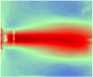
Figure 2. The PIV measurements of horizontal velocity fields in the  $x_{\ast }$ direction at three times,
  $t/T_0$, normalized with the wave beam period
  $T_0 = 2{\rm \pi} /\omega = 14$ s: (a) 20; (b) 40; (c) 100. The left-hand images show the wave beam responses in the vertical plane
  $z_{\ast } = 0$, while the middle and right-hand images depict the induced mean flow in the vertical plane
  $z_{\ast } = 0$ and the horizontal plane
  $y_{\ast } = 0$, respectively. These planes are indicated by dashed lines. The thick black line marks the location of the wave generator. The zero-velocity line around
  $x=10$ cm in the right-hand images is an experimental artifact due to laser sheet reflection.
Figure 2 reveals that the wave beam response has essentially reached steady state by  $t/T_0 = 20$ and changes very little thereafter. This is in sharp contrast to the induced mean flow, which at early times is confined in the region of the generated wave beam (figure 2a), but later starts to spread in the
  $x_{\ast }$ direction (figure 2b), and eventually reaches a quasi-steady state that stretches along the
  $x_{\ast }$ direction far away from the beam (figure 2c). It should be noted that the mean flow is purely horizontal (i.e. negligible in the
  $y_{\ast }$ direction) and also features a component in the
  $z_{\ast }$ direction (not shown here) as required by incompressibility. At late times, however, when the mean flow is highly elongated in the
  $x_{\ast }$ direction relative to the
  $z_{\ast }$ direction (figure 2c), the transverse (
 $z_{\ast }$) component is much smaller than the along-tank (
 $x_{\ast }$) component.
Previous experiments using a similar set-up (Bordes Reference Bordes2012; Bordes et al. Reference Bordes, Venaille, Joubaud, Odier and Dauxois2012) concentrated on the beam–mean-flow interaction while the induced mean flow still resides in the vicinity of the wave beam (figure 2a). This early stage is characterized by rapid growth (linear in time) of the mean PV associated with the horizontal mean flow, which also affects the underlying internal wave beam as indicated by the cross-beam bending of the beam profile in figure 2 (left-hand images). The focus here, however, is on the long-time mean-flow development (figure 2b,c).
3. Extended mean-flow equation
Previous closely related theoretical work (Kataoka & Akylas Reference Kataoka and Akylas2015; Fan et al. Reference Fan, Kataoka and Akylas2018) focused on PV production and its pivotal role in mean-flow generation by a three-dimensional internal wave beam in a stratified Boussinesq fluid. Fan et al. (Reference Fan, Kataoka and Akylas2018), in particular, considered a weakly nonlinear nearly monochromatic wave beam and derived two coupled evolution equations for the beam envelope and the induced mean flow, assuming that three-dimensional variations are weak; namely, that the ratio of the cross-beam length scale  $\lambda _{\ast }/2{\rm \pi}$ (where
  $\lambda _{\ast }$ is the beam carrier wavelength) to a characteristic transverse beam length scale
  $W_{\ast }$,
 \begin{equation} \varepsilon= \frac{\lambda_{\ast}}{2{\rm \pi} W_{\ast}}, \end{equation}
is small ( $\varepsilon \ll 1$). The mean-flow evolution equation in this model, however, applies only to the early stage of the mean-flow development, which is dominated by the production of mean PV in the vicinity of the beam. To capture the mean-flow dynamics at later times, here we propose an extended mean-flow evolution equation that, in addition, accounts for the advection of mean PV by the induced mean flow as well as for the viscous diffusion of mean PV in the far field away from the beam. Although negligible at early times, these effects control the long-time mean-flow dynamics brought out by the experimental observations (figure 2b,c).
3.1. Onset of streaming
We begin by reviewing the model of Fan et al. (Reference Fan, Kataoka and Akylas2018). Their analysis focused on the ‘distinguished limit’ where the nonlinear beam–mean-flow coupling is as important as the effects of the along-beam dispersion, transverse dispersion and viscous attenuation of the beam envelope. For the benefit of readers interested in a detailed discussion of the scalings appropriate to this flow regime, we adopt the same non-dimensionalization (with  $1/N$ as the time scale, where
  $N$ is the constant buoyancy frequency, and
  $\lambda _{\ast }/2{\rm \pi}$ as the length scale, where
  $\lambda _{\ast }$ is the beam carrier wavelength set by the wave generator) and use the same notation as Fan et al. (Reference Fan, Kataoka and Akylas2018). Here, as our interest centres on the experiments in § 2, background rotation is ignored (
 $\,f=0$).
In terms of  $\varepsilon \ll 1$ defined in (3.1), which controls the assumed weak transverse variations, the beam envelope and the induced mean flow depend on the ‘slow’ spatial variables
 \begin{equation} X=\varepsilon^{2}\xi,\quad Y=\varepsilon \eta,\quad Z=\varepsilon z, \end{equation}
where  $\xi$,
  $\eta$ and
  $z$ are the along-beam, cross-beam and transverse coordinates, respectively (figure 3). Referring to the experimental set-up (figure 1), the coordinate system
  $\mathrm {O}xyz$ in figure 3 is the non-dimensional counterpart of
  $\textrm {O}_\ast x_{\ast }y_{\ast }z_{\ast }$, and the
  $(\xi ,\eta )$ coordinates are rotated by
  $\theta$ relative to the horizontal and vertical
  $(x,y)$ coordinates. Furthermore, the appropriate ‘slow’ time is
 \begin{equation} T=\varepsilon^{2} t, \end{equation}
indicating that the initial phase of the mean-flow development lasts  $O(1/\varepsilon ^{2})$ beam periods.

Figure 3. Schematic of theoretical model for the generated wave beam. The coordinate system  $\mathrm {O}xyz$ is the non-dimensional counterpart of
  $\textrm {O}_\ast x_{\ast }y_{\ast }z_{\ast }$ (figure 1),
  $y$ is the upward vertical and
  $x$ and
  $z$ are the along-tank and transverse horizontal coordinates, respectively. The along- and cross-beam coordinates
  $\xi$ and
  $\eta$ (also marked in figure 1) are rotated by
  $\theta$ relative to
  $(x,y)$. The beam has a nearly monochromatic profile. Dotted lines indicate lines of constant phase of the sinusoidal carrier whose wavelength (set by the wave generator) has been normalized to
  $2{\rm \pi}$ in the asymptotic analysis. The envelope scale is
  $O(\varepsilon ^{-2})$ along the
  $\xi$ direction and
  $O(\varepsilon ^{-1})$ along the
  $\eta$ and
  $z$ directions, in keeping with the scalings (3.2a–c).
At this stage, the disturbance comprises an  $O(\varepsilon )$ primary harmonic, representing a weakly nonlinear nearly monochromatic beam, and an
  $O(\varepsilon ^{2})$ mean flow. Specifically, the velocity components
  ${\boldsymbol u}=(u,v,w)$ in the
  $(\xi ,\eta ,z)$ coordinate system, the density perturbation
  $\rho$ and the pressure perturbation
  $p$ take the form
 \begin{gather} {\boldsymbol u}=\varepsilon \{ {(U,\varepsilon^{2}V,\varepsilon W)\,\mbox{e}^{{\mathrm{i}}\varphi }+\mbox{c.c.}} \}+ \varepsilon^{2}(\bar{{U}},\bar{{V}},\bar{{W}})+\cdots, \end{gather}
 \begin{gather}\rho =\varepsilon \{ {R\,\mbox{e}^{{\mathrm{i}}\varphi }+\mbox{c.c.}} \}+\varepsilon^{4}\bar{{R}}+\cdots,\quad p=\varepsilon \{{P\,\mbox{e}^{{\mathrm{i}}\varphi}+\mbox{c.c.}}\}+\varepsilon^{3}\bar{{P}}+\cdots, \end{gather}
where  $\varphi =\eta -\omega t$ and
  $\omega =\sin \theta$. (These perturbation expansions are somewhat different from (2.11) in Fan et al. (Reference Fan, Kataoka and Akylas2018) owing to our assumption of no rotation,
  $f=0$; details of the analysis for
  $0\le f \ll 1$ including the scaling of the mean flow above can be found in Fan (Reference Fan2017).) The coupled beam–mean-flow dynamics is described via the various amplitudes in (3.4), which depend on
  $X$,
$X$,  $Y$,
$Y$,  $Z$ and
  $T$. The equations governing these amplitudes are obtained by imposing incompressibility, mass conservation and momentum balance. Specifically, upon substituting (3.4) into these fundamental equations and collecting terms
  $\propto \exp ( {\mathrm {i}}\varphi )$, the beam amplitudes can be expressed in terms of the along-beam velocity amplitude
  $U$:
$U$:
 \begin{equation} V={\mathrm{i}} U_{X} +\cot \theta U_{ZZ},\quad W=-{\mathrm{i}}\cot \theta U_{Z},\quad R=-{\mathrm{i}} U,\quad P=\cos \theta U. \end{equation}
Thus, in view of (3.2a–c) and (3.4a), the beam response obeys incompressibility correct to  $O(\varepsilon ^3)$. Furthermore, to the same order of approximation,
  $U$ satisfies the evolution equation
 \begin{equation} U_{T} +{\mathrm{i}}\bar{V}U+\cos \theta \left({U_{X} -\frac{{\mathrm{i}}}{2}\cot \theta U_{ZZ} } \right)+ \frac{\beta }{2}U=0. \end{equation}
The second term in (3.6) is the feedback of the induced mean flow to the beam dynamics, while the third and fourth terms, respectively, account for the effects of (along-beam and transverse) dispersion and viscous attenuation of the beam envelope. This balance of dissipation with nonlinear coupling and dispersion assumes that the inverse Reynolds number  $\nu =4{\rm \pi} ^2 \nu _{\ast }/N {\lambda _{\ast }}^2$ scales like
 \begin{equation} \nu =\beta \varepsilon^{2}, \end{equation}
where  $\beta =O(1)$.
Turning next to the induced mean flow, from mass conservation it is deduced that the vertical velocity is  $O(\varepsilon ^{4})$. Thus, to leading order, the mean flow is purely horizontal:
 \begin{equation} \bar{U}=\bar{V}\cot \theta. \end{equation}
Furthermore, as along-beam variations are weaker than cross-beam and transverse variations in view of (3.2a–c), incompressibility to leading order requires
 \begin{equation} \bar{V}_{Y} +\bar{W}_{Z} =0. \end{equation}
Finally, to complete the description of the beam–mean-flow interaction, we find it convenient to utilize the transport equation
 \begin{equation} q_{t} +{\boldsymbol u}\boldsymbol{\cdot} \boldsymbol{\nabla} q=\nu ({\nabla^{2}\zeta -\boldsymbol{\nabla} \rho \boldsymbol{\cdot} \nabla^{2}(\boldsymbol{\nabla} \times {\boldsymbol u})}) \end{equation}
for the PV
 \begin{equation} q=\zeta -\boldsymbol{\nabla} \rho \boldsymbol{\cdot} (\boldsymbol{\nabla} \times {\boldsymbol u}), \end{equation}
where  $\zeta =(\boldsymbol {\nabla } \times {\boldsymbol u})\boldsymbol {\cdot } {\boldsymbol j}$ is the vertical vorticity and
  ${\boldsymbol j}$ denotes the vertical (
 $y$) unit vector. From (3.11), upon making use of (3.4)–(3.5a–d), it follows that
  $q=\varepsilon ^{3}\bar {Q}+\cdots ,$ where
 \begin{equation} \bar{Q}=\varOmega -2(UU^{\ast })_{Z} \end{equation}
is the mean PV amplitude and
 \begin{equation} \varOmega =\frac{1}{\sin \theta }\bar{V}_{Z} -\sin \theta \bar{W}_{Y} \end{equation}
is the amplitude of the mean vertical vorticity,  $\zeta =\varepsilon ^{3}\varOmega +\cdots$. Thus, taking into account (3.4), (3.7), (3.12) and (3.13), the balance of mean terms in the PV transport equation (3.10), correct to
  $O(\varepsilon ^{5})$, yields
 \begin{equation} \varOmega_{T} =2\left({\frac{\partial }{\partial T}+\beta } \right)(UU^{\ast })_{Z}. \end{equation}
This evolution equation along with (3.6), (3.9) and (3.13), which govern the beam–mean-flow interaction for  $T=O(1)$, are the end results of Fan et al. (Reference Fan, Kataoka and Akylas2018).
It should be noted that the vertical vorticity associated with the induced mean flow derives from two separate sources, one of inviscid and the other of viscous origin, corresponding to the two contributions to the forcing term on the right-hand side of (3.14). The focus here is on the mean flow due to the viscous source of vertical vorticity: this mean flow component, referred to as streaming, is forced resonantly and eventually overwhelms its inviscid counterpart. Specifically, for  $T=O(1)$, the beam amplitude
  $U$, governed by (3.6), reaches a quasi-steady state. Thus, in response to the viscous forcing term in (3.14),
  $\varOmega$ grows linearly in
  $T$,
$T$,
 \begin{equation} \varOmega \sim 2\beta T(UU^{\ast })_{Z}, \end{equation}
and so do  $\bar {V}$ and
  $\bar {W}$. As a result, the convective derivative term on the left-hand side of the PV transport equation (3.10), which does not partake in the
  $O(\varepsilon ^5)$ dominant balance leading to (3.14), eventually comes into play.
3.2. Saturation of streaming
As noted above, the dominant balance of  $O(\varepsilon ^5)$ terms in (3.10) that provides the mean vorticity equation (3.14) eventually is invalidated owing to the resonant growth of streaming. Specifically, this breakdown occurs at
  $T=O(\varepsilon ^{-1/2})$, when
  $\bar {V}$ and
  $\bar {W}$ are of
  $O(\varepsilon ^{-1/2})$ so the convective derivative term is as important as the time evolution term in (3.10). Thus, to bring out the proper balance of mean terms in (3.10) when
  $T=O(\varepsilon ^{-1/2})$, we introduce the rescaled mean-flow variables
 \begin{equation} (\bar{V}, \bar{W}) \to \varepsilon^{-1/2} (\bar{V}, \bar{W}),\quad \varOmega \to \varepsilon^{-1/2} \varOmega, \end{equation}
which depend on  $X$,
$X$,  $Y$,
$Y$,  $Z$ defined in (3.2a–c) and the rescaled slow time
 \begin{equation} \hat{T}= \varepsilon^{1/2} T. \end{equation}
Upon implementing these scalings in the PV transport equation (3.10), equation (3.14) for the mean vertical vorticity is replaced by
 \begin{equation} \left({\frac{\partial }{\partial \hat{T}}} +\bar{V} {\frac{\partial }{\partial Y}} + \bar{W} {\frac{\partial }{\partial Z}} \right) \varOmega =2 \beta(UU^{\ast})_{Z} . \end{equation}
In this evolution equation, the advection by the induced mean flow counterbalances the viscous forcing of  $\varOmega$. Thus, the resonant growth (3.15) predicted at early times (
 $\hat {T} \ll 1$) is expected to saturate for
  $\hat {T}=O(1)$ and, as a result, the mean flow would level off and start being transported away from the beam region. Qualitatively, this scenario is consistent with the experimental observations presented in § 2.2: the growth of streaming in the beam vicinity is essentially complete after 20 beam periods (figure 2a), and by 40 periods (figure 2b) the effects of advection are clearly visible. Detailed comparison between theory and experiments is made in § 4.
3.3. Far-field flow regime
As the mean vertical vorticity continues to be transported away from the beam, the effect of the forcing term on the right-hand side of (3.18) gradually diminishes. Thus, for  $\hat {T} \gg 1$ the mean flow far from the beam reaches a quasi-steady state due to the balance of horizontal advection with viscous diffusion in the PV transport equation (3.10). In this far-field regime, as revealed by the experimental observations (figure 2c), the mean flow is highly elongated in the horizontal (
 $x$) direction. This suggests replacing the beam-oriented variables
  $X=\varepsilon ^{2} \xi$ and
  $Y=\varepsilon \eta$ in (3.2a–c) with
  $x$ and
  $y$ (see figure 3), scaled such that
  $x$ variations are weaker than vertical (
 $y$) and transverse (
 $z$) variations. Additionally, the far-field flow scalings should bring out the anticipated balance of horizontal advection with viscous diffusion of the mean PV.
The scaled spatial variables appropriate to the far field are
 \begin{equation} \tilde{X}=\varepsilon^{5/2} x, \quad \tilde{Y}=\varepsilon y, \quad Z=\varepsilon z. \end{equation}
It should be noted that  $\tilde {X}$ is ‘slower’ than
  $\tilde {Y}$ and
  $Z$ in keeping with the observed far-field characteristics of the mean flow (figure 2c), while
  $Z$ remains as in (3.2a–c) to permit matching with the near field as
  $\tilde {X} \to 0$. Furthermore, as
  $\tilde {X}$ is scaled differently from
  $Z$, it becomes necessary to rescale the transverse (
 $z$) mean-flow velocity,
 \begin{equation} \bar{W} \to \varepsilon^{3/2} \bar{W}, \end{equation}
so as to satisfy incompressibility
 \begin{equation} \frac{1}{\sin \theta }\bar{V}_{\tilde{X}} +\bar{W}_{Z} =0. \end{equation}
In view of the rescaling (3.20), in the far field the  $z$-velocity component
  $\varepsilon ^3 \bar {W}$ is smaller than the
  $x$-velocity component
  $\varepsilon ^{3/2} \bar {V}/\sin \theta$, which as noted in § 2.2 is also consistent with our experimental observations. Thus, the amplitude of the mean vertical vorticity to leading order is given by
 \begin{equation} \varOmega=\frac{\bar{V}_{Z}}{\sin \theta}. \end{equation}
Finally, returning to (3.10), in view of (3.19a–c) and (3.20), the dominant balance of mean PV terms in the far field yields
 \begin{equation} \left({\frac{\partial }{\partial \tilde{T}}+\frac{\bar{V}}{\sin \theta } \frac{\partial }{\partial \tilde{X}}+\bar{W}\frac{\partial }{\partial Z}-\beta \left({\frac{\partial^{2}}{\partial \tilde{Y}^{2}}+\frac{\partial^{2}}{\partial Z^{2}}} \right)}\right)\varOmega =0, \end{equation}
where
 \begin{equation} \tilde{T}= \varepsilon^{3/2} \hat{T} = \varepsilon^2 T= \varepsilon^4 t \end{equation}
is the ‘very slow’ time appropriate to the mean-flow dynamics at this late stage. As expected, the evolution equation (3.23) accounts for the horizontal advection and viscous diffusion of  $\varOmega$, which are the main controlling factors in the far field.
3.4. Combined mean-flow equation
To investigate quantitatively the three stages of mean-flow dynamics identified above, it would be necessary to solve the evolution equations (3.14), (3.18) and (3.23), subject to appropriate initial and matching conditions. Considering that these problems would have to be tackled numerically, we find it more convenient instead to work with a single mean-flow evolution equation that combines the dominant effects in the three flow regimes. This extended equation reduces asymptotically to the simpler evolution equations (3.14), (3.18) and (3.23), respectively, under the appropriate flow scalings for  $T$,
$T$,  $\hat {T}$ and
  $\tilde {T}=O(1)$.
Specifically, since the mean flow is horizontal to leading order, we introduce a streamfunction  $\varPsi (\chi ,\tilde {Y},Z,T)$, where
  $(\chi ,\tilde {Y},Z)=\varepsilon (x,y,z)$ and
  $T=\varepsilon ^2 t$, such that the mean-flow velocity components in (3.4a) are given by
 \begin{equation} \bar{V}= \sin\theta \varPsi_{Z},\quad \bar{W}=-\varPsi_{\chi}, \end{equation}
with  $\bar {U}= \cos \theta \varPsi _{Z}$ according to (3.8). Thus,
 \begin{equation} \frac{1}{\sin \theta }\bar{V}_{\chi} +\bar{W}_{Z} =0, \end{equation}
which ensures that the incompressibility equations (3.9) and (3.21) are satisfied automatically in the corresponding flow regimes. Furthermore, in view of (3.25a,b), the mean vertical vorticity takes the form
 \begin{equation} \varOmega =\frac{1}{\sin \theta }\bar{V}_{Z} -\bar{W}_{\chi}=\varPsi_{\chi\chi} +\varPsi_{ZZ}, \end{equation}
which reduces asymptotically to expressions (3.13) and (3.22) under the corresponding flow scalings. Finally, the evolution equations (3.14), (3.18) and (3.23) can be combined to the following transport equation for  $\varOmega$:
 \begin{equation} \varOmega_{T} +\varepsilon J(\varOmega,\varPsi) -\varepsilon^2 \beta \left({\frac{\partial^{2}}{\partial \tilde{Y}^{2}}+\frac{\partial^{2}}{\partial Z^{2}}} \right) \varOmega=2\left({\frac{\partial }{\partial T}+\beta } \right)(UU^{\ast })_{Z}, \end{equation}
where  $J(a,b)\equiv a_{\chi } b_{Z} -a_{Z} b_{\chi }$.
Setting  $\varepsilon =0$ in (3.28) recovers the evolution equation (3.14) derived in Fan et al. (Reference Fan, Kataoka and Akylas2018) that is valid at the early stage of mean-flow generation,
  $T=O(1)$, when the production of mean PV due to the underlying modulated beam is the dominant effect. At the later times
  $\hat {T}=O(1)$ and
  $\tilde {T}=O(1)$, the
  $O(\varepsilon )$ and
  $O(\varepsilon ^2)$ terms in (3.28), which account for the effects of advection and viscous diffusion of mean PV, respectively, come into play as discussed above. The extended mean-flow equation (3.28) along with (3.25a,b), (3.27) and the beam evolution equation (3.6) comprise the theoretical model to be used below for quantitative comparison against our experimental observations and numerical Navier–Stokes simulations.
4. Comparison of theory with experiments
The proposed theoretical model of beam–mean-flow dynamics is now applied to the experiments in § 2. As in Fan et al. (Reference Fan, Kataoka and Akylas2018), we choose the transverse width ( $=\!3.7\lambda _{\ast }$) of the wave generator as
  $W_{\ast }$ in (3.1) so
  $\varepsilon =0.043$. Thus, in view of (3.2a–c), the wave generator width is normalized to
  $Z=1$ while the generator height (
 $=\!3\lambda _{\ast }$) is equal to 0.8 in terms of
  $Y$, and the viscous parameter
  $\beta =15.6$ according to (3.7). Furthermore, to account for the forcing due to the horizontally moving plates of the generator at the left-hand wall of the tank, we prescribe at
  $X=0$ the envelope of the along-beam wave beam velocity, in the form
 \begin{align} U &= A_{0} \left\{ {\tanh \left[ {15(Y+0.4)} \right]-\tanh \left[ {15(Y-0.4)} \right]} \right\}\nonumber\\ &\quad \times \left\{ {\tanh \left[{5(Z+0.5)} \right]-\tanh \left[ {5(Z-0.5)} \right]} \right\}/4, \end{align}
where  $A_0$ controls the peak forcing amplitude. The smoothing coefficients in tanh functions are the same as in Fan et al. (Reference Fan, Kataoka and Akylas2018) and correspond to the best agreement with experiments. The boundary forcing (4.1) is applied at
  $T=0$, and the resulting beam–mean-flow response for
  $T>0$ is determined by integrating the evolution equations (3.6) and (3.28) along with (3.25a,b) and (3.27), starting from the quiescent state
  $U=\varOmega =0$.
The above initial–boundary-value problem is solved numerically via pseudo-spectral discretization in  $-4.0<Y<4.0$,
  $-3.0<Z<3.0$ and second-order centred finite differences in
  $0<X<0.32$, combined with fourth-order Runge–Kutta time stepping. The parameter
  $A_0$ in (4.1) is chosen such that the integral in the central vertical plane (
 $Z=0$) of the
  $x$-component of mean flow at 20 beam periods matches the value of this integral obtained from the experimental mean flow data at the same time. The results reported here were computed using
  $128\times 64$ Fourier modes in
  $Y \times Z$, 128 grid points in
  $X$ and
  ${\rm \Delta} T=8.0\times 10^{-4}$.
Apart from the experimental results, the proposed theoretical model is also compared against numerical simulations based on the full Navier–Stokes equations. Referring to the experimental set-up (figure 1), these simulations use no-slip boundary conditions on the tank bottom and walls, except the left-hand wall ( $x_{\ast }=0$), where at
  $t=0$ we apply the forcing due to the wave generator (located in
  $-5.7\ {\rm cm}< y_{\ast }<5.7\ \mathrm {cm}$,
  $-7.0\ {\rm cm} < z_{\ast } <7.0\ \mathrm {cm}$). This is done by prescribing the horizontal velocity in the
  $x_{\ast }$ direction in the form
 \begin{align} u_{\ast } &= U_{0} \frac{\mathrm{d} x_{\ast}}{\mathrm{d}t} \{ {\tanh [ {2.2 \left(y_{\ast }+5.7 \right)}]-\tanh [ {2.2(y_{\ast }-5.7)}]} \}\nonumber\\ &\quad \times \{ {\tanh [ {2.2(z_{\ast }+7.0)} ]-\tanh [ {2.2(z_{\ast }-7.0)}]}\}/4 \quad (x_{\ast}=0), \end{align}
with  $\mathrm {d} x_{\ast }/\mathrm {d}t$ determined from (2.1). Furthermore, similar to
  $A_0$ in (4.1), the forcing amplitude parameter
  $U_0$ in (4.2) is chosen such that the integral in the central vertical plane (
 $z_{\ast }=0$) of the numerically computed mean-flow velocity in the
  $x_{\ast }$ direction at 20 beam periods matches the value of this integral based on the experimental mean-flow data at the same time. The Navier–Stokes equations are solved numerically by adapting to the present three-dimensional geometry the procedure outlined in Kataoka & Akylas (Reference Kataoka and Akylas2020) for two-dimensional reflection of an internal wave beam from a rigid slope. The results reported here were obtained using the computational domain
  $x_{\ast } \times y_{\ast } \times z_{\ast }=107\ \mathrm {cm}\times 38\ \mathrm {cm}\times 80\ \mathrm {cm}$ with
  $120\times 150\times 100$ grid points and the time step
  ${\rm \Delta} t=0.07$ s. The grid points were more concentrated near the wave generator in order to achieve higher resolution there. Finally, results are unchanged when using larger values of coefficients in tanh functions in (4.2).
Figures 4 and 5 show horizontal velocity fields in the  $x_{\ast }$ direction obtained from the theoretical model and Navier–Stokes simulations under the same flow conditions as for the experimental results in figure 2. These plots of beam and mean-flow responses allow direct comparison of the theoretical (figure 4) and numerical (figure 5) predictions against the experimental observations (figure 2) at
  $t/T_0 =20$, 40 and 100. These snapshots are representative of the three regimes of beam–mean-flow dynamics discussed in § 3 – the genesis of streaming in the beam vicinity (figures 2a, 4a, 5a), the beginning of mean-flow advection along the horizontal (figures 2b, 4b, 5b) and the balance of horizontal advection with viscous diffusion in the far-field mean-flow response (figures 2c, 4c, 5c). The theoretical model reproduces these flow regimes and captures all the salient features of the observations and simulations. The time instants
  $t/T_0 =20$, 40 and 100 chosen above also are consistent with the characteristic time scales
  $t \sim 1/\varepsilon ^2$,
  $1/\varepsilon ^{5/2}$ and
  $1/\varepsilon ^4$ of the three mean-flow regimes discussed in § 3, if the cross-beam length scale
  $\lambda _{\ast }/2{\rm \pi}$ is replaced with
  $\lambda _{\ast }$ in the definition of
  $\varepsilon$ in (3.1), so that
  $\varepsilon =0.27$ instead of 0.043. (The length scale
  $\lambda _{\ast }/2{\rm \pi}$ is used here in order to match the non-dimensional variables of Fan et al. (Reference Fan, Kataoka and Akylas2018); while
  $2{\rm \pi}$ is an
  $O(1)$ constant asymptotically, it can make an appreciable difference numerically when computing order-of-magnitude estimates.)

Figure 4. Horizontal velocity fields in the  $x_{\ast }$ direction obtained from the theoretical model at three time instants: (a)
  $t/T_0 =20$; (b)
  $t/T_0 =40$; (c)
  $t/T_0 =100$. The flow snapshots here are direct counterparts of the experimental images displayed in figure 2 and the numerical simulations in figure 5.

Figure 5. Horizontal velocity fields in the  $x_{\ast }$ direction obtained from Navier–Stokes numerical simulations at three time instants: (a)
  $t/T_0 =20$; (b)
  $t/T_0 =40$; (c)
  $t/T_0 =100$. The flow snapshots here are direct counterparts of the experimental images displayed in figure 2 and the theoretical model predictions in figure 4.
It should be noted that in the theoretical model the boundary forcing (4.1) is applied in terms of the (scaled) cross-beam coordinate  $Y=\varepsilon \eta$, which is rotated relative to the vertical
  $y$ by
  $\theta$ (figure 3), and the tank bottom is ignored. This explains the small gap of the theoretical responses near the wave generator and the absence of beam reflections at the tank bottom in figure 4. These minor discrepancies, however, do not detract from the overall excellent agreement of the theoretical model with the experiments and simulations. Furthermore, similar agreement among theoretical, experimental and numerical responses is found for the other two driving frequencies we considered, which correspond to
  $\theta =15^\circ$ and
  $45^\circ$.
We also made quantitative comparison between theory and experiments of the time evolution of the induced mean flow, for the three driving frequencies corresponding to the beam propagation angles  $\theta =15^\circ$,
  $30^\circ$ and
  $45^\circ$. Specifically, figure 6 shows plots for
  $0<t/T_0 <120$ (where
  $T_0$ is the beam period) of the maximum mean-flow velocity in the
  $x_{\ast }$ direction (figure 6a) and the integrated mean vertical vorticity in the horizontal quarter plane
  $0<x_{\ast }<\infty$,
  $0<z_{\ast }<\infty$ through the centre of the wave generator (figure 6b). These plots compare the predictions of the present theoretical model against those of the model by Fan et al. (Reference Fan, Kataoka and Akylas2018) as well as our experimental observations and Navier–Stokes simulations. In all cases, the integrated mean vertical vorticity is estimated by computing the integral of the horizontal mean flow in the
  $x_{\ast }$ direction along the centreline
  $y_{\ast }=z_{\ast }=0$ and
  $0<x_{\ast } <65\ \mathrm {cm}$.

Figure 6. Time evolution of induced mean flow for  $0<t/T_0<120$, where
  $T_0=2{\rm \pi} /\omega$ is the beam period, for the driving frequencies
  $\omega =0.24$, 0.45 and 0.64 rad s
 $^{-1}$, corresponding to the beam propagation angles
  $\theta =15^{\circ }$,
  $30^{\circ }$ and
  $45^{\circ }$, respectively. Comparison of the present theoretical model (solid curve) against the model of Fan et al. (Reference Fan, Kataoka and Akylas2018) (dotted curve), Navier–Stokes simulations (dashed curve) and experiments (circles). (a) Maximum mean-flow velocity in the along-tank (
 $x_{\ast }$) direction; (b) integrated mean vertical vorticity.
According to figure 6, there is overall excellent agreement of the present model with the experiments and numerical simulations. In contrast, the model of Fan et al. (Reference Fan, Kataoka and Akylas2018) is reliable for limited time only. This discrepancy is more pronounced for the maximum mean-flow velocity in figure 6(a), which clearly highlights the three stages of mean-flow dynamics: (i) onset of streaming ( $t/T_0 \lesssim 20$), when the maximum mean-flow velocity grows resonantly (linearly in time); (ii) saturation of streaming (
 $20 \lesssim t/T_0 \lesssim 40$); and (iii) establishment of a quasi-steady state (
 $t/T_0 \gtrsim 40$). As expected, the model of Fan et al. (Reference Fan, Kataoka and Akylas2018) captures only (i). Furthermore, figure 6(a) reveals that for
  $\theta =15^\circ$ the maximum mean-flow velocity saturates to about half the value it reaches for
  $\theta =30^\circ$ and
  $45^\circ$. This explains why in previous experiments the refraction effects on the wave beam due to the mean flow were less apparent for
  $\theta =15^\circ$ (Bordes et al. Reference Bordes, Venaille, Joubaud, Odier and Dauxois2012) than
  $\theta =28^\circ$ (Bordes Reference Bordes2012).
5. Concluding remarks
Mean-flow generation by a three-dimensional internal gravity wave beam in a stratified fluid hinges on two distinct mechanisms: viscous production of mean PV which gives rise to streaming, and material conservation of mean PV which is responsible for an inviscid modulation-induced mean flow. Under the experimental flow conditions of Bordes (Reference Bordes2012) and Bordes et al. (Reference Bordes, Venaille, Joubaud, Odier and Dauxois2012), production of mean PV in the beam vicinity dominates, and the observed mean flow is of the streaming type as evidenced by the mean vertical vorticity which grows linearly in time. In addition, however, these experiments suggest that horizontal advection of mean PV plays a part in the mean-flow dynamics after some time, leading to saturation of streaming, an effect beyond the reach of the model of Fan et al. (Reference Fan, Kataoka and Akylas2018).
With this hint as our motivation, we conducted experiments using a set-up similar to that of Bordes (Reference Bordes2012) and Bordes et al. (Reference Bordes, Venaille, Joubaud, Odier and Dauxois2012), but with forcing acting for longer times, in order to understand the ultimate fate of streaming. The new observations confirm that horizontal advection of mean PV by the growing mean flow eventually does come into play and causes streaming to saturate. Furthermore, as a result of the mean flow being advected away from the beam region, finally a quasi-steady state is established in the far field. The mean flow in this far-field response is highly elongated in the along-tank horizontal direction due to a balance of horizontal advection with viscous diffusion of mean PV.
To explain theoretically the mean-flow development revealed by our experiments, we revisited the asymptotic model of Fan et al. (Reference Fan, Kataoka and Akylas2018) and included the effects of horizontal advection and viscous diffusion of mean PV which control the long-time mean-flow dynamics. The extended asymptotic analysis confirms the three stages of mean-flow dynamics brought out by the experiments: genesis of streaming due to resonant mean PV production in the beam vicinity at early times, followed by saturation of streaming due to horizontal advection of mean PV and finally the establishment of a quasi-steady state in the far field due to viscous diffusion of mean PV. The predictions of the revised model are in remarkably good agreement with the experimental observations and numerical simulations based on the full Navier–Stokes equations. Thus, for an internal wave beam, it is possible to trace theoretically the entire evolution of streaming observed experimentally.
Acknowledgements
The authors thank G. Pillet for preliminary experiments and S. Joubaud and P. Odier for insightful discussions. This work was supported by the Labex iMUST (ANR-10-LABX-0064) of Université de Lyon, within the programme ‘Investissements d'Avenir’ (ANR-11-IDEX-0007), operated by the French National Research Agency (ANR), France, and by the ANR through grant ANR-17-CE30-0003 (DisET). One of the authors (T.R.A.) also acknowledges support from the US National Science Foundation through grant DMS-1512925. This work was made possible thanks to the resources of PSMN from ENS de Lyon.
Declaration of interests
The authors report no conflict of interest.


