


1. Introduction
Thin liquid films are integral to our daily lives and innumerable industrial applications. The physics of thinning and rupture of liquid films with two free surfaces, which are referred to as liquid sheets or free liquid films, plays a critical role in foam evolution (Cohen-Addad, Höhler & Pitois Reference Cohen-Addad, Höhler and Pitois2013), drop coalescence and emulsion stability (Loewenberg & Hinch Reference Loewenberg and Hinch1996; Yoon et al. Reference Yoon, Baldessari, Ceniceros and Leal2007; Sambath et al. Reference Sambath, Garg, Thete, Subramani and Basaran2019; Anthony, Harris & Basaran Reference Anthony, Harris and Basaran2020), as well as in applications involving bubbles bursting at interfaces (Stewart et al. Reference Stewart, Feng, Kimpton, Griffiths and Stone2015). Similarly, the thinning dynamics of films supported by a solid substrate, with one free surface, is crucial in applications as diverse as coating flows (Christodoulou & Scriven Reference Christodoulou and Scriven1989; Weinstein & Ruschak Reference Weinstein and Ruschak2004), tear film substitutes (Braun Reference Braun2012), heat transfer (Lohse & Villermaux Reference Lohse and Villermaux2020) and pattern formation (Mukherjee & Sharma Reference Mukherjee and Sharma2015). Moreover, a number of technologically important free surface flows, for example, curtain coating which arises in coating flow applications, involve both free and supported films where the integrity of both types of films is crucial for the successful practice of the operation (Kistler & Scriven Reference Kistler and Scriven1983; Bazzi & Carvalho Reference Bazzi and Carvalho2019).
If the thickness of such films is of or less than the order of a micrometre, long-range intermolecular forces become significant and influence the thinning dynamics (De Gennes Reference De Gennes1985; Kheshgi & Scriven Reference Kheshgi and Scriven1991). For thin sheets, van der Waals attraction between the two free surfaces can cause spontaneous thinning and eventual rupture of the film despite the presence of stabilizing capillary pressure. A striking example of sheet rupture can be found in the paper by Debrégeas, De Gennes & Brochard-Wyart (Reference Debrégeas, De Gennes and Brochard-Wyart1998) who observed it while studying experimentally the bursting of bubbles at air–liquid interfaces. These authors reported that the sheet that forms between the bubble and the interface spontaneously ruptures below a thickness of 70 nm due to van der Waals attraction. Similarly, for thin films on a substrate, van der Waals attraction between the liquid–gas interface and the solid substrate can lead to spontaneous thinning of the film and the subsequent formation of dry spots (Reiter Reference Reiter1992; Stange, Evans & Hendrickson Reference Stange, Evans and Hendrickson1997; Becker et al. Reference Becker, Grün, Seemann, Mantz, Jacobs, Mecke and Blossey2003). When these intermolecular forces are significant, they are accounted for in the analysis of dynamics of film thinning and rupture by the addition of a disjoining pressure term to the set of governing equations (Teletzke, Davis & Scriven Reference Teletzke, Davis and Scriven1987). The goal of this work is to advance the understanding of the thinning and rupture of liquid sheets or free films that are surrounded by a dynamically inactive ambient fluid when the film liquid is non-Newtonian and its response can be characterized by power-law rheology.
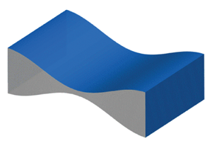
Consider a liquid sheet of uniform thickness  $2h_0$ that is surrounded by a passive gas such as air (figure 1). In what follows, it is taken that the midplane of the sheet lies in the
  $\tilde {x}$–
 $\tilde {z}$-plane of a rectangular coordinate system and the
  $\tilde {y}$-axis is perpendicular to the midplane. Here, pressure variations due to gravity are negligible due to the thinness of the sheet. Next, consider that the two surfaces of the sheet are perturbed symmetrically about its midplane by shape perturbations that are invariant or translationally symmetric in the
  $\tilde {x}$-direction such that the shape and/or location of the free surface
  $\tilde {y} = \tilde {h}(\tilde {z})$ that lies above the
  $\tilde {x}$–
 $\tilde {z}$-plane is given by
 \begin{equation} \tilde{h} (\tilde{z}) = h_0 \left[1 - \epsilon \cos \left(\frac{{\rm \pi} \tilde{z}}{\tilde{\lambda}}\right)\right], \end{equation}
while the shape of the free surface below is given by the negative of (1.1). Here,  $\epsilon \ll 1$ is the amplitude and
  $\tilde {\lambda }$ is the wavelength of the perturbation. As is well known (Thete et al. Reference Thete, Anthony, Doshi, Harris and Basaran2016; Zheng et al. Reference Zheng, Fontelos, Shin, Dallaston, Tseluiko, Kalliadasis and Stone2018), capillary pressure due to surface tension
  $\sigma$, which is given by
  $\sigma (\partial ^2 {\tilde {h}}/\partial {\tilde {z}}^2)$, is stabilizing and tries to return the sheet to its original flat or planar profile. As is also well known, disjoining pressure due to van der Waals attraction, which is given by
  $A_H/[6{\rm \pi} (2\tilde {h})^3]$ (
 $A_H$, Hamaker constant), is destabilizing and acts to grow the perturbation. A simple scaling argument reveals that for the two forces to balance,
  $\tilde {z} \sim \tilde {h}^2/d$, where
  $d \equiv (A_H/2{\rm \pi} \sigma )^{1/2}$ is the molecular length scale for the particular liquid–gas system, and, therefore, long-wavelength disturbances are destabilizing. Ruckenstein & Jain (Reference Ruckenstein and Jain1974) performed a more exact linear stability analysis and determined that liquid sheets that are subjected to perturbations of wavelengths exceeding a critical value
  $\tilde {\lambda }_c$ are always unstable, where the value of the critical wavelength is given by
 \begin{equation} \tilde{\lambda}_c = \frac{8{\rm \pi}^{3/2}\sigma^{1/2}{h_0}^{2} }{A_H^{1/2}}= {4\sqrt{2}{\rm \pi}}\frac{h_0}{d}h_0. \end{equation}
Typically,  $h_0 \gg d$ as
  $h_0$ is of the order of micrometres whereas
  $d$ is a few nanometres, which implies that the critical wavelength for spontaneous rupture is much larger than the initial film thickness
  $({\tilde {\lambda }}_c \gg h_0)$, a result that accords with the simple scaling argument carried out above. Thus, thin free films or sheets are unstable to long-wavelength perturbations.

Figure 1. A liquid sheet or a free film undergoing line rupture: definition sketch. (a) Perspective view of a liquid sheet that is surrounded by a dynamically passive fluid like air. The sheet is shown over a distance in the lateral  $(\tilde {z})$ direction corresponding to one wavelength
  $\tilde {\lambda }$ of the shape perturbation imposed at the interface(s). (b) A cross-sectional view of the film. Highlighted here is the so-called ‘rupture zone’ in the vicinity of the location where the sheet will break and the dynamics is expected to be self-similar as the space–time singularity is approached. (c) Because of the underlying symmetries, the computational domain is simply the region that is shaded in grey in the figure.
Erneux & Davis (Reference Erneux and Davis1993) made use of the long-wavelength nature of the problem and solved a set of one-dimensional (1-D) partial differential equations (PDEs) for the film thickness and lateral velocity as a function of the lateral spatial coordinate  $\tilde {z}$ and time
  $\tilde {t}$ for Newtonian sheet rupture. They determined that nonlinear effects led to acceleration of thinning and resulted in rupture times well below those predicted by linear theory. Given the separation of scales between the dynamics of the macroscopic film and that occurring in the vicinity of the location where the film breaks (which is sometimes referred to as the rupture zone or the hot zone), the dynamics of film thinning is self-similar in the vicinity of the space–time singularity (
 $\tilde {z} = \tilde {z}_R, \tilde {t} = \tilde {t}_R$), where
  $\tilde {z}_R$ and
  $\tilde {t}_R$ are the lateral location and time at which the film thickness vanishes (
 $\tilde {h} = 0$) and the sheet ruptures (Barenblatt Reference Barenblatt1996). Moreover, the separation of scales also leads to the expectation that the dynamics of sheet rupture is universal such that it is independent of initial and boundary conditions imposed on the macroscopic film (Barenblatt Reference Barenblatt1996). In pioneering work, Ida & Miksis (Reference Ida and Miksis1996) explored the self-similar dynamics of thinning of a viscous Newtonian sheet, and determined that the dominant force balance is between viscous and van der Waals forces, while inertial and capillary forces are subdominant. Subsequently, in a paper of central importance in the field, Vaynblat, Lister & Witelski (Reference Vaynblat, Lister and Witelski2001) carried out an analytical and numerical study of Newtonian liquid sheets undergoing both line – translationally symmetric or two-dimensional – and point – axisymmetric – rupture. These authors solved both the set of spatially 1-D, transient PDEs or evolution equations for sheet thickness
  $\tilde {h}$ and lateral velocity
  $\tilde {v}$ in physical space as well as a set of ordinary differential equations (ODEs) for these variables in similarity space. These authors thereby demonstrated that the eventual asymptotic dynamical balance of forces for both point and line rupture is between van der Waals force, viscous force and inertia, with surface tension force being negligible. They also demonstrated excellent agreement between self-similar solutions determined from solving the PDEs and analytical solutions of the aforementioned ODEs. In this inertial–viscous (IV) regime, these authors showed that the film half-thickness
  $\tilde {h}$, lateral length scale
  $\tilde {z}^{\prime }$ and lateral velocity
  $\tilde {v}$ vary with time remaining until rupture
  $\tilde {\tau } \equiv \tilde {t}_R - \tilde {t}$ as
 \begin{equation} \tilde{h} \sim \tilde{\tau}^{1/3},\quad \tilde{z}^{\prime} \sim \tilde{\tau}^{1/2},\quad \tilde{v} \sim \tilde{\tau}^{{-}1/2}, \end{equation}
where  $1/3$,
  $1/2$ and
  $-1/2$ are referred to as the scaling exponents. More recently, our group (Thete et al. Reference Thete, Anthony, Doshi, Harris and Basaran2016) studied the dynamics of thinning of Newtonian sheets when the Ohnesorge number
  $Oh \equiv \mu _0/\sqrt {\rho h_0 \sigma }$ is varied, where
  $\rho$ is the density of the film fluid and
  $\mu _0$ is its viscosity (
 $Oh$ is a dimensionless group that denotes the ratio of viscous force to the square root of the product of inertial and capillary forces) and, in particular, in the limit when inertia is negligible (
 $Oh^{-1} = 0$) and that when viscosity is negligible (
 $Oh = 0$). We demonstrated that in the limit of
  $Oh^{-1}=0$ or when the sheet is undergoing Stokes flow, the dynamics lies in the aforementioned viscous (V) regime discovered by Ida & Miksis (Reference Ida and Miksis1996) where the dominant force balance is between viscous and van der Waals forces, and capillary force is always negligible. The resulting dynamics gives rise to self-similarity of the second kind (Barenblatt Reference Barenblatt1996) and where the scaling exponents are given by
 \begin{equation} \tilde{h} \sim \tilde{\tau}^{1/3},\quad \tilde{z}^{\prime} \sim \tilde{\tau}^{0.26},\quad \tilde{v} \sim \tilde{\tau}^{{-}0.74}. \end{equation}
In a previous work (Thete et al. Reference Thete, Anthony, Doshi, Harris and Basaran2016), we obtained the scaling exponent for the lateral length scale of  $\beta = 0.26$ independently through numerical simulations of the 1-D PDEs and analytical solutions of the 1-D ODEs in similarity space. For inviscid sheets or when
  $Oh = 0$, we showed that the dominant force balance is between inertial, van der Waals and capillary forces, and the scaling exponents in this inertial–capillary (IC) regime are given by
 \begin{equation} \tilde{h} \sim \tilde{\tau}^{2/7},\quad \tilde{z}^{\prime} \sim \tilde{\tau}^{4/7},\quad \tilde{v} \sim \tilde{\tau}^{{-}3/7}. \end{equation}
Equally importantly, we showed in Thete et al. (Reference Thete, Anthony, Doshi, Harris and Basaran2016) that for real fluids for which  $Oh$ is finite, the V and IC regimes are transitory and the dynamics will always asymptotically transition to the late-stage IV regime discovered by Vaynblat et al. (Reference Vaynblat, Lister and Witelski2001). In this previous paper (Thete et al. Reference Thete, Anthony, Doshi, Harris and Basaran2016), we also determined analytically the film thickness at which these transitions occur and demonstrated excellent agreement between theory and numerical simulations for the values of film thickness at which transitions between different scaling regimes take place.
While the studies discussed above have focused on sheets of Newtonian fluids, many fluids encountered in industrial applications and daily life exhibit more complex rheology. An important type of such non-Newtonian fluids is the so-called power-law fluid, which derives its name from the power-law dependence (Deen Reference Deen1998) of the viscosity  $\tilde {\mu }$ on the deformation rate
  $\tilde {\dot \gamma }$ given by
 \begin{equation} \tilde\mu(\tilde{\dot\gamma}) = {\mu}_0\left|2\tilde{m}\tilde{\dot \gamma}\right|^{n-1}. \end{equation}
Here,  $\mu _0$ is the zero-deformation-rate viscosity,
  $\tilde {m}^{-1}$ the characteristic deformation rate,
  $0< n\le 1$ the power-law exponent or index (
 $n = 1$ corresponds to a Newtonian fluid) of the given fluid and
  $\tilde {\dot \gamma }$ is the second invariant of the rate-of-deformation tensor
  $\tilde {\boldsymbol {D}}$, which is referred to as the deformation rate
 \begin{gather} \tilde{\dot \gamma} = \left[\frac{1}{2}(\tilde{\boldsymbol{D}} : \tilde{\boldsymbol{D}})\right]^{{1}/{2}}, \end{gather}
 \begin{gather} \tilde{\boldsymbol{D}} = \frac{1}{2}[(\tilde{\boldsymbol{\nabla}} \tilde{\boldsymbol{v}}) + (\tilde{\boldsymbol{\nabla}} \tilde{\boldsymbol{v}})^{\rm T} ], \end{gather}
where  $\tilde {\boldsymbol {v}}$ is the fluid velocity. Experimental studies have shown that many common fluids exhibit power-law rheology (Hasan, Ghannam & Esmail Reference Hasan, Ghannam and Esmail2010; Savage et al. Reference Savage, Caggioni, Spicer and Cohen2010; Huisman, Friedman & Taborek Reference Huisman, Friedman and Taborek2012; Bonn et al. Reference Bonn, Denn, Berthier, Divoux and Manneville2017).
The self-similar dynamics and finite-time singularities that arise when the working liquids are power-law fluids have been studied extensively in situations involving the pinch-off of liquid threads (jets) and such studies are of particular relevance to the present paper. Scaling exponents and similarity solutions derived analytically in pinch-off of power-law threads (Renardy Reference Renardy2002; Doshi et al. Reference Doshi, Suryo, Yildirim, McKinley and Basaran2003; Doshi & Basaran Reference Doshi and Basaran2004) have been verified against numerical simulations of the 1-D slender jet equations (Doshi et al. Reference Doshi, Suryo, Yildirim, McKinley and Basaran2003; Doshi & Basaran Reference Doshi and Basaran2004) and, in some cases, the full three-dimensional axisymmetric equations (Suryo & Basaran Reference Suryo and Basaran2006) and even experiments (Savage et al. Reference Savage, Caggioni, Spicer and Cohen2010; Huisman et al. Reference Huisman, Friedman and Taborek2012). Until recently, studies of thin-film flows of power-law fluids had focused on the dynamics of films on cylinders (Gorla Reference Gorla2001), films on rotating discs (Arora & Doshi Reference Arora and Doshi2016), tear films in our eyes (Zhang, Matar & Craster Reference Zhang, Matar and Craster2003) and flow of films down inclined planes (Miladinova, Lebon & Toshev Reference Miladinova, Lebon and Toshev2004) without delving into the self-similar dynamics of van der Waals-driven rupture. In our previous work (Thete et al. Reference Thete, Anthony, Basaran and Doshi2015), we examined the rupture of sheets of power-law fluids of  $Oh = O(1)$ and demonstrated that for fluids with
  $6/7 < n \le 1$, the dynamics followed the power-law inertial–viscous (PLIV) scaling theory, for which the power-law scalings are given by
 \begin{equation} \tilde{h} \sim \tilde{\tau}^{n/3},\quad\tilde{z}^{\prime} \sim \tilde{\tau}^{1-n/2},\quad \tilde{v} \sim \tilde{\tau}^{{-}n/2}. \end{equation}
It is noteworthy that the scaling exponents in this PLIV regime depend on the rheology of the fluid, viz. they are functions of the power-law index  $n$. However, when
  $0 < n \le 6/7$, it was demonstrated by Thete et al. (Reference Thete, Anthony, Basaran and Doshi2015) that viscous forces drop out of the dominant force balance: the balance in this range of
  $n$ is between inertial, van der Waals and capillary forces, which leads to the IC regime from (1.5a–c). In other words, for
  $0 < n \le 6/7$, the sheet for all practical purposes behaves as if it were inviscid because the fluid's local viscosity in the vicinity of the rupture singularity falls rapidly as the singularity is approached and the thinning dynamics becomes rheology independent. However, while our earlier work (Thete et al. Reference Thete, Anthony, Basaran and Doshi2015) deciphered the local dynamics of thinning for sheets of power-law fluids of
  $Oh = O(1)$, the response of highly viscous or slightly viscous sheets has remained heretofore unexplored. More recently, we demonstrated in Garg et al. (Reference Garg, Kamat, Anthony, Thete and Basaran2017) that a similar transition from a capillary–viscous to an inertial–capillary regime occurs for thin films of power-law fluids on a substrate, and determined the critical values of the governing parameters at which this transition should be observed. In our recent paper on rupture of Newtonian sheets (Thete et al. Reference Thete, Anthony, Doshi, Harris and Basaran2016), it is specifically stated that there is a need for a comprehensive study of the thinning of sheets of power-law fluids. Such a study, which would parallel the already existing studies of pinch-off of threads of power-law fluids (Suryo & Basaran Reference Suryo and Basaran2006), would (i) provide a thorough understanding of the rupture dynamics of liquid sheets, which is at present incomplete, and (ii) determine all transitions that occur between different scaling regimes in the parameter space comprised of both the Ohnesorge number
  $Oh$ and power-law exponent
  $n$. Accomplishing these aforementioned goals is the main objective of this paper.
The paper is organized as follows. Section 2 describes the problem under investigation, and presents the equations and boundary conditions governing the thinning of liquid sheets. Furthermore, in this section, a succinct description is provided of the numerical methods used to solve the set of two-dimensional (2-D) PDEs and the set of 1-D PDEs that is employed for analytically investigating the self-similar dynamics of sheet rupture. Section 3 analyses theoretically and computationally the thinning and rupture of sheets of power-law fluids when inertia is negligible, i.e. when the film is undergoing Stokes flow or  $Oh^{-1} = 0$. Section 4 briefly explains why thinning dynamics in the inviscid limit, or when
  $Oh = 0$, is identical for Newtonian and power-law sheets. Section 5 analyses thinning and rupture of sheets of real fluids where
  $Oh$ is finite for the entire range of power-law exponent values of
  $0 < n \le 1$. In contrast to Newtonian films (Thete et al. Reference Thete, Anthony, Doshi, Harris and Basaran2016), it is demonstrated that a remarkably richer array of transitions is observed for power-law fluids. Additionally, a detailed exploration is carried out to uncover transitions between scaling regimes for highly viscous and slightly viscous sheets. Section 6 provides a summary of the key findings and outlines fruitful avenues of future research. In Appendix A, results are also presented for situations in which liquid sheets of power-law fluids are subjected to initial perturbations of finite-amplitude and highlights that short wavelength perturbations can be detrimental to the integrity of thin free films when their amplitudes are sufficiently large.
2. Mathematical formulation
The system is an isothermal free film or sheet of uniform thickness  $2h_0$ of an incompressible power-law liquid of constant density
  $\rho$ and zero-deformation-rate viscosity
  $\mu _0$. The film is surrounded by a dynamically passive gas such as air that exerts a constant pressure, set equal to zero without loss of generality, and negligible viscous drag on the film. The Hamaker constant
  $A_H$ for the liquid–gas system and the surface tension of the interface
  $\sigma$ are constant and spatially uniform. It proves convenient here to use a rectangular coordinate system
  $(\tilde {x}, \tilde {y}, \tilde {z})$: the origin of the coordinate system is located in the midplane that lies half-way between and is parallel to the two undisturbed surfaces of the sheet, and the three coordinates are such that the
  $(\tilde {x}, \tilde {z})$-plane coincides with the midplane and
  $\tilde {y}$ is the coordinate that runs in the direction perpendicular to that plane (see figure 1a). Below, the
  $\tilde {z}$-direction is also referred to as the lateral direction and the
  $\tilde {y}$-direction as also the vertical direction. The fluid within the film of uniform thickness
  $2h_0$ is initially quiescent, but at time
  $\tilde {t} = 0$, its two surfaces are subjected to a sinusoidal perturbation such that the half-thickness of the film and/or the shape of its top surface,
  $\tilde {y} = \tilde {h}(\tilde {z}, \tilde {t})$, at
  $\tilde {t} = 0$, is given by (1.1). As this perturbation is spatially periodic in the lateral (
 $\tilde {z}$) direction and translationally symmetric or invariant in the
  $\tilde {x}$-direction, we hereafter restrict our analysis to the evolution of the sheet profile and the flow within it to the 2-D domain whose lateral extent equals half of a wavelength of the imposed perturbation (
 $0 \le \tilde {z} \le \tilde {\lambda }/2$). Thus, the problem domain is the region bounded above by the free surface
  $\tilde {S} (\tilde {t})$ which is unknown a priori, bounded below by the midplane of the film located at
  $(\tilde {y} = 0, 0 \le \tilde {z} \le \tilde {\lambda }/2)$, and bounded on the sides by the symmetry planes located at
  $\tilde {z} = 0$ and
  $\tilde {z} = \tilde {\lambda }/2$, as shown in figure 1(c). The effect of gravity is assumed to be negligible on account of the film's thinness. In what follows, we first describe the spatially 2-D, transient Cauchy momentum and continuity equations that govern the thinning and rupture of films of power-law fluids and the numerical methods used to solve these equations. We then describe the set of spatially 1-D transient PDEs that are employed to analyse the self-similar behaviour of sheet rupture theoretically by making use of the long wavelength nature of the problem.
2.1. Governing equations and 2-D formulation
In formulating the dimensionless equations governing film thinning and rupture and the 2-D algorithm used to solve them, the problem variables are non-dimensionalized by using the undisturbed film half-thickness as the characteristic length,  $l_c \equiv h_0$, the visco-capillary time as the characteristic time,
  $t_c \equiv \mu _0 h_0/\sigma$, the ratio of these two scales as the characteristic velocity,
  $v_c \equiv l_c/t_c$, the zero-deformation-rate viscosity as the characteristic viscosity
  $\mu _c \equiv \mu _0$ and the capillary pressure as the characteristic pressure
  $p_c \equiv \sigma /h_0$. As a result of choosing these characteristic scales, the dynamics is governed by four dimensionless groups (see below): the Ohnesorge number,
  $Oh \equiv {\mu _0}/(\rho \sigma h_0)^{1/2}$, which represents the ratio of the viscous force to the square root of the product of the inertial and capillary forces; the van der Waals number,
  $A \equiv A_H/48 {\rm \pi}\sigma {h_0}^2$, which represents the relative importance of intermolecular forces to capillary forces; the power-law exponent or index
  $n$; and the characteristic deformation rate,
  $m^{-1} = t_c {\tilde {m}}^{-1}$. For the remainder of this paper, variables without tildes
  $(\sim )$ over them represent the dimensionless counterparts of the corresponding dimensional variables with tildes over them, e.g.
  $\tilde {z}$ is the dimensional lateral coordinate whereas
  $z \equiv \tilde {z}/l_c$ is its dimensionless counterpart.
The dynamics of the liquid sheet is governed by the continuity and Cauchy momentum equations which are given in dimensionless form by
 \begin{equation} \boldsymbol{\nabla} \boldsymbol{\cdot} {\boldsymbol v} = 0, \end{equation}
 \begin{equation} \frac{1}{Oh^2} \left ( \frac {\partial {\boldsymbol v}}{\partial t} + {\boldsymbol v} \boldsymbol{\cdot} \boldsymbol{\nabla} {\boldsymbol v} \right ) = \boldsymbol{\nabla} \boldsymbol{\cdot} {\boldsymbol T}. \end{equation}
Here,  $\boldsymbol {\nabla } \equiv h_0 \tilde {\boldsymbol {\nabla }}$ is the dimensionless gradient operator,
  $\boldsymbol v \equiv \tilde {\boldsymbol {v}} /v_c = v_y \boldsymbol {e_y} + v_z \boldsymbol {e_z}$ is the dimensionless liquid velocity, where
  $v_y$ and
  $v_z$ are the
  $y$- and
  $z$-components of
  $\boldsymbol v$ and
  $\boldsymbol {e_y}$ and
  $\boldsymbol {e_z}$ are the unit vectors in those directions,
  $t \equiv \tilde {t}/ t_c$ is the dimensionless time, and
  ${\boldsymbol T} = - p {\boldsymbol I} + \mu [ \boldsymbol {\nabla } \boldsymbol v + (\boldsymbol {\nabla } \boldsymbol v)^{\rm T} ]$ is the dimensionless stress tensor, where
  $p \equiv \tilde {p}/p_c$ is the dimensionless pressure and
  $\mu = |2m \dot \gamma |^{n-1}$ is the dimensionless viscosity with
  $\dot \gamma \equiv \tilde {\dot \gamma } t_c$ denoting the dimensionless deformation rate.
The kinematic and traction boundary conditions are applied at the liquid–gas interface  $S(t)$ to enforce mass conservation and to account for the discontinuity or jump in stress due to surface tension and van der Waals forces:
 \begin{gather} \boldsymbol n \boldsymbol{\cdot} \left ( {\boldsymbol v} - {\boldsymbol v}_s \right ) = 0, \end{gather}
 \begin{gather} \boldsymbol n \boldsymbol{\cdot} {\boldsymbol T} = 2{H}\boldsymbol n - \frac {A}{h^3}\, \boldsymbol{n}, \end{gather}
where  ${\boldsymbol v}_s$ is the velocity of points on the interface
  $S( t)$,
  $\boldsymbol {n}$ is the unit normal vector to
  $S(t)$ and
  $2{H}$ is twice the mean curvature of
  $S(t)$. Symmetry boundary conditions are enforced at the two symmetry planes located at
  $z = 0$ and
  $z = {\lambda }/2$ by requiring that the lateral velocity and tangential stress equal zero. Finally, along the midplane located at
  $y = 0$, the vertical velocity and tangential stress both vanish on account of symmetry.
The film is initially quiescent, and the wavelength of the perturbations  ${\lambda }$ imposed on its two free surfaces are taken to be larger than the dimensionless critical wavelength obtained from linear stability analysis and given by
  ${\lambda }_c = {4 \sqrt {2}{\rm \pi} ^{3/2}}{h_0}/{d}$. Thus, the film in its initial configuration is unstable and thereafter thins continuously until it ruptures. Because the dynamics in the rupture zone is insensitive to the values of the amplitude
  $\epsilon$ and wavelength
  $\lambda$ of the interface perturbation when
  $\lambda > \lambda _c$ and
  $\epsilon \ll 1$, these two parameters are not included in the list of dimensionless groups governing the dynamics in the body of the paper. However, we address briefly the effects of perturbation amplitude and wavelength on the dynamics in Appendix A. Following earlier studies of pinch-off singularities discussed in the introduction, we adopt in the next few sections the universally practiced usage of reporting results as a function of dimensionless time
  $\tau \equiv (\tilde {t}_R - \tilde {t})/t_c$ remaining until rupture (but also see below).
2.2. Numerical methods for solving the 2-D equations
The 2-D free surface flow governed by the PDEs (2.1)–(2.2) subject to the aforementioned boundary and initial conditions is solved using a fully implicit, method of lines (MOL), arbitrary Langrangian–Eulerian (ALE) algorithm. Here, the Galerkin/finite element method (G/FEM) is used for spatial discretization (Feng & Basaran Reference Feng and Basaran1994) and a predictor–corrector method with an adaptive, implicit finite difference scheme is employed for time integration (Wilkes, Phillips & Basaran Reference Wilkes, Phillips and Basaran1999).
Two features of the flow make the spatial discretization challenging. First, the film's free surfaces undergo large deformations as the sheet approaches rupture. Second, because  $h_0 \gg d$, the lateral extent of the domain is three to five orders of magnitude larger than its vertical extent. Therefore, to capture the large deformations that the film's surface
  $S(t)$ undergoes and to accurately capture the dynamics that occurs over highly disparate length scales in the lateral and vertical directions, the elliptic mesh generation method (Christodoulou & Scriven Reference Christodoulou and Scriven1992; Notz & Basaran Reference Notz and Basaran2004) is used to discretize the domain and determine the vertical and lateral coordinates of each grid point in the moving, adaptive mesh simultaneously with the velocity and pressure unknowns within the liquid sheet. Here, the velocity and pressure unknowns are solved in a mixed interpolation scheme where the nodal values of the velocity are represented in terms of biquadratic basis functions while the pressure unknowns are represented by means of bilinear basis functions. The unknown coordinates of the grid or mesh points are also represented by biquadratic basis functions.
The PDEs are converted to ODEs by the G/FEM formulation while time integration reduces the system of ODEs to a system of nonlinear algebraic equations. These are solved using Newton's method with an analytically computed Jacobian. The linearized system of equations at each iteration is solved using a multi-frontal algorithm (Anthony et al. Reference Anthony, Kamat, Harris and Basaran2019). Variants of this algorithm have been employed by our research group to successfully study hydrodynamic singularities that arise in thread pinchoff of both Newtonian and non-Newtonian fluids (Yildirim & Basaran Reference Yildirim and Basaran2001; Notz & Basaran Reference Notz and Basaran2004; Suryo & Basaran Reference Suryo and Basaran2006; Bhat et al. Reference Bhat, Appathurai, Harris, Pasquali, McKinley and Basaran2010; Castrejón-Pita et al. Reference Castrejón-Pita, Castrejón-Pita, Thete, Sambath, Hutchings, Hinch, Lister and Basaran2015; Kamat et al. Reference Kamat, Wagoner, Thete and Basaran2018), drop and bubble coalescence (Paulsen et al. Reference Paulsen, Burton, Nagel, Appathurai, Harris and Basaran2012; Munro et al. Reference Munro, Anthony, Basaran and Lister2015; Anthony et al. Reference Anthony, Kamat, Thete, Munro, Lister, Harris and Basaran2017), and rupture of supported thin films (Garg et al. Reference Garg, Kamat, Anthony, Thete and Basaran2017). The reader is thus referred to these works for a more complete description of the solution method and numerical implementation.
2.3. 1-D equations for asymptotic analysis
To study sheet dynamics analytically, the long-wavelength approximation (Deen Reference Deen1998; Leal Reference Leal2007) can be invoked to reduce the system of 2-D PDEs (2.1)–(2.2) to a set of 1-D PDEs for the film thickness and lateral velocity. These 1-D PDEs governing thinning and rupture of power-law films have already been derived by Thete et al. (Reference Thete, Anthony, Basaran and Doshi2015). In this paper, we are interested in studying the dynamics of sheets in both the Stokes and the inviscid limits in which the governing equations can be obtained by formally setting the density  $\rho = 0$ (or equivalently the reciprocal of the Ohnesorge number
  $1/Oh = 0$) in the former case and the viscosity
  $\mu _0=0$ (or equivalently
  $Oh=0$) in the latter case. Thus, it turns out to be necessary to non-dimensionalize the 1-D evolution equations in two different ways such that (a) one formulation is suitable for studying the dynamics when
  $Oh \gg 1$ and, in particular, in the limit of
  $1/Oh = 0$ and (b) the other formulation is appropriate for studying the dynamics when
  $Oh \ll 1$ and, in particular, in the limit of
  $Oh = 0$.
2.3.1. 1-D evolution equations: highly viscous sheets
For highly viscous sheets, the 1-D PDEs governing the dynamics are non-dimensionalized by using  $l_c \equiv h_0$ as the characteristic length in the vertical direction and
  $l_z \equiv (48 {\rm \pi}{h_0}^4 \sigma /A_H )^{1/2}$ as the characteristic length in the lateral direction, which incorporates the disparity of the vertical and the lateral length scales into the formulation from the outset. Also in this limit, we use
  $t_V \equiv 48 {\rm \pi}{h_0}^3 \mu _0/A_H$ as the characteristic time and
  $v_V \equiv l_z/t_V$ as the characteristic velocity. The characteristic time used here is related to the one used earlier in the 2-D formulation as
  $t_V \equiv t_c/A$. The dimensionless 1-D evolution equations are then given by
 \begin{gather} \frac{\partial h}{\partial t} + \frac{\partial \left( h v \right)}{\partial z} = 0, \end{gather}
 \begin{gather} \frac{1}{Oh^2}\underbrace{\left(\frac{\partial v}{\partial t} + v \frac {\partial v} {\partial z} \right)}_{\text{Inertial (I)}} = \underbrace{\frac{\partial^3 h}{\partial { z}^3}}_{\text{Capillary (C)}} + \underbrace{\frac{\partial \left( { h}^{{-}3} \right)}{\partial { z}}}_{\text{van der Waals (vdW)}} + \underbrace{\frac{4}{ h} \frac {\partial}{\partial z} \left({\mu_V} {h} \frac {\partial v}{\partial z} \right)}_{\text{Viscous (V)}}. \end{gather}
Here,  $z \equiv \tilde {z} / l_z$ is the dimensionless lateral length,
  $t \equiv \tilde {t}/t_V$ is the dimensionless time,
  $h ( z, t )$ denotes the dimensionless film half-thickness,
  $v ( z, t )$ denotes the dimensionless fluid velocity in the lateral or
  $z$ direction and
  $\mu _V = {|2 m_1 {\partial v}/{\partial z} |}^{n-1}$, where
  $m_1$ is related to
  $m$ in the 2-D formulation as
  $m_1 = mA$. The different forces that influence van der Waals-driven rupture of sheets, namely inertial (I), capillary (C), van der Waals (vdW) and viscous (V) forces, are identified by labels placed under each of the corresponding terms in (2.6).
2.3.2. 1-D evolution equations: slightly viscous sheets
For slightly viscous sheets, the 1-D PDEs governing the dynamics are non-dimensionalized by using  $l_c \equiv h_0$ as the characteristic length in the vertical direction and
  $l_z \equiv (48 {\rm \pi}{h_0}^4 \sigma /A_H )^{1/2}$ as the characteristic length in the lateral direction which, once again, recognizes the disparity of length scales in the two directions from the beginning. The characteristic length scales in the two directions used in this limit are thus the same as those used for highly viscous sheets. In this limit, however, since viscosity should not be involved in defining characteristic scales, we use
  $t_I \equiv ({\rho l_z^4}/{\sigma h_0})^{1/2}$ as the characteristic time and
  $v_I \equiv l_z/t_I$ as the characteristic velocity. The characteristic time used here is related to the one used in the 2-D formulation as
  $t_I = t_c/(Oh \, A)$. The dimensionless 1-D evolution equations are then given by
 \begin{gather} \frac{\partial h}{\partial t} + \frac{\partial \left( h v \right)}{\partial z} = 0, \end{gather}
 \begin{gather} \underbrace{\left(\frac{\partial v}{\partial t} + v \frac {\partial v} {\partial z} \right)}_{\text{Inertial (I)}} = \underbrace{\frac{\partial^3 h}{\partial { z}^3}}_{\text{Capillary (C)}} + \underbrace{\frac{\partial \left( { h}^{{-}3} \right)}{\partial { z}}}_{\text{van der Waals (vdW)}} + \underbrace{\frac{4 Oh}{ h} \frac {\partial}{\partial z} \left({\mu_I} {h} \frac {\partial v}{\partial z} \right)}_{\text{Viscous (V)}}. \end{gather}
Here,  $z \equiv \tilde {z} / l_z$ is the dimensionless lateral length,
  $t \equiv \tilde {t}/t_I$ is the dimensionless time,
  $h ( z, t )$ denotes the dimensionless film half-thickness,
  $v ( z, t )$ denotes the dimensionless fluid velocity in the lateral or
  $z$ direction and
  $\mu _I = {|2 m_2 {\partial v}/{\partial z} |}^{n-1}$, where
  $m_2$ is related to
  $m$ in the 2-D formulation as
  $m_2 = m \, Oh \, A$. The different forces that influence van der Waals-driven rupture of sheets have once again been identified by labels placed under each of the corresponding terms in (2.8).
2.3.3. Local analyses and similarity variables
The film thickness and velocity profiles are expected to be self-similar in the vicinity of the location where the film thickness is minimum as the space–time singularity is approached. In § 3, we explore the dynamical behaviour of the film thickness and lateral velocity in this so-called ‘rupture zone’, which is shown in figure 1(b), by numerical solution of the 2-D system of (2.1)–(2.2) and theoretical analysis of the 1-D system of equations that have just been presented (see §§ 2.3.1 and 2.3.2).
In the 1-D analysis, we presume that the film half-thickness  $h(z,t)$ and the lateral velocity
  $v(z,t)$ can be represented by adopting the similarity ansatz
 \begin{equation} h \equiv \tau_*^{\alpha}H(\xi), \quad v \equiv \tau_*^{\gamma}V(\xi),\quad \xi \equiv \zeta / \tau_*^{\beta}, \end{equation}
where  $\tau _* \equiv (\tilde {t}_R - \tilde {t})/t_*$ is the dimensionless time remaining until rupture and
  $t_*$ is a characteristic time, with both
  $\tau _*$ and
  $t_*$ being defined differently depending on whether the sheet is highly or slightly viscous (see below). Here,
  $\xi$ is the similarity variable,
  $\zeta \equiv (\tilde {z} - \tilde {z}_R)/l_z$ is the dimensionless lateral coordinate relative to the rupture point,
  $\alpha$,
  $\beta$ and
  $\gamma$ are the scaling exponents, and
  $H(\xi )$ and
  $V(\xi )$ are the scaling functions for the film thickness profile and lateral velocity in similarity space. When using the non-dimensionalization adopted with the 1-D analysis for highly viscous sheets and, in particular, when analysing the Stokes limit (
 $1/Oh^2=0$ in (2.6)), we denote
  $\tau _*$ by
  $\tau _V$ and note that
  $t_* \equiv t_V$, viz.
  $\tau _v \equiv (\tilde {t}_R - \tilde {t})/t_V$ (the use of subscripts ‘
 $V$’ is intended to highlight that we are in a highly viscous regime). Similarly, when using the non-dimensionalization adopted with the 1-D analysis for slightly viscous sheets and, in particular, when analysing the inviscid limit (
 $Oh=0$ in (2.8)), we denote
  $\tau _*$ by
  $\tau _I$ and note that
  $t_* \equiv t_I$ (the use of subscripts ‘
 $I$’ is intended to highlight that we are in a slightly viscous or nearly inviscid regime). We note the three dimensionless times remaining until rupture are related as
  $\tau _V = A \tau$ and
  $\tau _I = Oh \, A\tau$.
3. Thinning dynamics in the Stokes limit
In this section, rupture of liquid sheets of power-law fluids is analysed in the limit  ${Oh^{-1} = 0}$ such that inertia is negligible and the sheet is undergoing purely viscous or Stokes flow. The governing 2-D equations in this limit are obtained by setting
  $1/Oh^2 = 0$ in (2.2) in the mathematical formulation presented in § 2.1 and the corresponding 1-D equations are obtained by setting
  $1/Oh^2 = 0$ in (2.6) in § 2.3.1.
Since Thete et al. (Reference Thete, Anthony, Doshi, Harris and Basaran2016) have shown for Newtonian sheets in the creeping flow limit that the dominant balance of forces is between van der Waals and viscous forces while capillary force is negligible, we begin with the hypothesis that the same dynamical balance holds for power-law sheets (but see below). Thus, substitution of (2.9a–c) into (2.5) and (2.6) reveals that the scaling exponents are given by
 \begin{equation} \alpha = n/3,\quad \gamma = \beta - 1, \end{equation}
where the relationship between  $\gamma$ and
  $\beta$ follows from the kinematic balance and the value of
  $\alpha$ follows from the dynamical balance that presupposes that capillary force is subdominant. According to (3.1a,b), as in the Newtonian limit
  $(n=1)$, the thinning dynamics exhibited by power-law sheets leads to self-similarity of the second kind (Barenblatt Reference Barenblatt1996) where the value of
  $\beta$, as shown below, must be determined as part of the solution.
If the dominant force balance is solely between van der Waals force that drives thinning and viscous force that resists it, it follows from (2.6) upon making use of the scaling exponents given in (3.1a,b) that the three forces, namely viscous (V), van der Waals (vdW) and capillary (C), vary with time remaining until rupture  $\tau _v$ as
 \begin{equation} V \sim vdW \sim \tau_v^{-\beta - n}, \quad C\sim \tau_v^{n/3 - 3\beta}. \end{equation}
It is clear from (3.2a,b) that in this regime, not only do viscous and van der Waals forces blow up as  $\tau _v \to 0$ as indicated, but that capillary force is negligible in comparison and hence is subdominant to the other two forces so long as the yet to be determined scaling exponent
  $\beta < 2n/3$. For Newtonian sheets
  $(n=1)$, Thete et al. (Reference Thete, Anthony, Doshi, Harris and Basaran2016) have shown that
  $\beta \doteq 0.26$ and this regime of sheet thinning is referred to as the viscous (V) regime. Thus, for Newtonian fluids, the inequality
  $\beta = 0.26 < 2n/3 = 2/3$ is satisfied, thereby justifying the neglect of capillary force in the dominant balance argument. We shall now investigate whether
  $\beta < 2n/3$ and the asymptotic behaviour of forces given in (3.2a,b) holds for all power-law sheets. In what follows, this regime of sheet thinning is referred to as the power-law viscous (PLV) regime. To accomplish this goal, we first numerically solve (2.1)–(2.2) subject to the boundary conditions and initial conditions as outlined in § 2 by subjecting the film to a perturbation of wavelength
  $\lambda = 2 \lambda _c$. It was determined by carrying out a number of simulations that subjecting the sheet to initial shape perturbations of wavelengths larger than this value had no effect whatsoever on the computed values of the scaling exponents or the behaviour of the solutions in the vicinity of the rupture location.
Figure 2 shows the variation with time remaining until rupture  $\tau$ of several variables of interest for a sheet of a power-law fluid of
  $n=0.9$ undergoing Stokes flow (the values of the other parameters are provided in the figure caption). The computational results shown in this figure and all the other figures in the remainder of this paper have been determined from 2-D simulations. These simulations and all others that have been carried out in this paper show that the value of the lateral coordinate of the liquid–gas interface
  $S(t)$ for which the film half-thickness is a minimum,
  $h_{min}$, is always located at
  $z = 0$. Moreover, in this case and in all others to be reported in this paper, the film ruptures at
  $z = z_R = 0$ so that
  $\zeta = z$ and asymptotically the interface profile is symmetric about this point as the sheet tends towards rupture. Figure 2(a) shows that according to the 2-D simulations,
  $h_{min}$ decreases with
  $\tau$ as
  $h_{min} = 0.0076{\tau }^{0.3}$. The value of the scaling exponent of 0.3 for the film thickness determined from the 2-D simulations agrees with the value of the scaling exponent predicted from theory, viz.
  $n/3 = 0.9/3$ (see 3.1a,b).

Figure 2. Scaling behaviour of variables in the rupture zone during thinning of a sheet undergoing Stokes flow. Here,  $n=0.9$,
  $A = 9.21 \times 10^{-8}$ and
  $m = 1/A$. The variation with time remaining until rupture
  $\tau$ of (a) the minimum film half-thickness
  $h_{min}$, (b) lateral length scale
  $z'$, evaluated at the lateral location where the film half-thickness is given by
  $h = 1.05 h_{min}$, and (c) lateral velocity
  $v'$ evaluated at the same lateral location as
  $z'$. The coloured data points correspond to results obtained from 2-D simulations while the black straight lines represent best fits to the data.
The 2-D simulations are also used to determine the value of the scaling exponent  $\beta$ for the lateral length scale or the lateral extent of the rupture zone
  $z'$. Here, the scaling of
  $z'$ is determined by tracking the lateral location of the film surface
  $S(t)$ where the film half-thickness
  $h$ equals some multiple of the minimum film half-thickness (Wagoner, Thete & Basaran Reference Wagoner, Thete and Basaran2018). Although the value of the scaling exponent is independent of the actual value of the multiple that is used (Suryo & Basaran Reference Suryo and Basaran2006), for definiteness sake, the value of
  $1.05 h_{min}$ is used here. The reason for determining the lateral length scale in this manner, as opposed to inferring it from the scaling of the curvature of the film profile which involves the second derivative of the interface shape function with respect to the lateral coordinate, has to do with the fact that we use the Galerkin finite element method in our simulations. In Galerkin and/or variational methods, one always carries out an integration by parts so that the highest order derivative in the resulting so-called weak form of the governing equations is first order. Therefore, second derivatives are never calculated nor used when employing weak formulations. Figure 2(b) shows that the 2-D simulation results predict that the lateral length scale varies with time to rupture as
  $z' \sim \tau ^{0.28}$, thus providing numerically that the value of the lateral scaling exponent, which was left undetermined from theory, is given by
  $\beta = 0.28$ when the power-law index
  $n=0.9$. Moreover, it was directly demonstrated that changing the value of the lateral location at which this determination is made, e.g. from
  $1.05 h_{min}$ to
  $1.1 h_{min}$, had no effect whatsoever on the value of
  $\beta$ that is predicted from the 2-D simulation results.
Figure 2(c) shows the variation with time remaining until rupture of the lateral velocity scale, which is hereafter referred to as  $v'$, that is predicted from 2-D simulations. Here,
  $v'$ is also evaluated at the lateral location where
  $h = 1.05 h_{min}$. As shown in figure 2(c), the lateral velocity can be seen to diverge as
  $\tau \to 0$ as
  $v' \sim \tau ^{-0.72}$, which is in excellent agreement with the scaling behaviour of
  $v'$ that is expected from theory, viz.
  $v' \sim \tau ^{\beta - 1} \sim \tau ^{0.28 - 1}$. The equality of the value of
  $\beta$, which is obtained directly from the computed variation of the lateral length scale
  $z'$ with
  $\tau$, and that which is obtained independently and indirectly from the computed scaling of
  $v'$ with
  $\tau$, after making use of the relationship
  $\beta = 1 - \gamma$, provides further credence to the accuracy of the numerically obtained value of
  $\beta = 0.28$ when the sheet is a power-law fluid of
  $n = 0.9$. Henceforward, the lateral length scale and lateral velocity scale are always computed at the lateral location where
  $h = 1.05 h_{min}$.
To gain further insights into the local dynamics of sheet rupture, we next derive and solve the ODEs in similarity space that govern the scaling functions  $H(\xi )$ and
  $V(\xi )$. We solve these ODEs in similarity space to determine independently the value of the lateral scaling exponent
  $\beta$ for a fluid of given
  $n$, to compute the value of the pre-factor in the expression that provides how
  $h_{min}$ varies with time remaining until rupture, and also to compare similarity solutions obtained from solving the 2-D PDEs in physical space with those obtained by solving these ODEs over the range
  $-\infty < \xi < \infty$. The ODEs and the boundary conditions to which they are subjected to along with the solution algorithm that is used to solve them, which is similar to that employed by Thete et al. (Reference Thete, Anthony, Doshi, Harris and Basaran2016) for Newtonian films, are described in detail in Appendix B.
As discussed in Appendix B, the determination of the lateral scaling exponent  $\beta$ from the analysis in similarity space entails the minimization of an error
  $\varepsilon _v$ in a certain velocity integral. Figure 3(a) shows the variation of this error
  $\varepsilon _v$ with
  $\beta$ for a power-law sheet of
  $n=0.9$. This figure makes plain that the error is minimized when
  $\beta = 0.28$, a result that is in excellent agreement with the value of
  $\beta$ obtained from 2-D simulations that are reported in figure 2(b). Furthermore, the value of
  $H_{0} \equiv H(0)$ obtained from the solution of the ODEs when
  $\beta = 0.28$ is
  $H_{0} = 0.986$. Since the film thickness is always a minimum at
  $\xi = \xi _0 = 0$, it can be seen from (2.9a–c) that
  $h_{min} = H_0 \tau _v^{n/3} = H_0 {A}^{n/3} \tau ^{n/3}$. Thus, given the value of
  $H_0$ that has just been determined from the solution of the ODEs, the pre-factor in the expression relating
  $h_{min}$ to
  $\tau$ is
  $H_0 {A}^{n/3} \equiv 0.0076$, which is in excellent agreement with the value obtained from the 2-D numerical solution as shown in figure 2(a). To compare the similarity solution for the interface shape obtained from the 1-D ODEs by the aforementioned shooting method and that from the numerical solution of the 2-D PDEs, the scaling function
  $H(\xi )$ is plotted along with the corresponding rescaled transient interface profile that has been obtained from the 2-D numerical simulations. In carrying out the comparison, the solution obtained from the ODEs is normalized as
 \begin{equation} \frac{h}{h_{min}} = \frac{H(\xi)}{H_0} \end{equation}
and plotted as a function of  $\xi$. Values of the local transient film half-thickness
  $h(z,t)$ obtained from 2-D numerical simulations, which of course correspond to the local values of the vertical
  $(y)$ coordinate of the liquid–gas interface
  $S(t)$, are similarly normalized as
 \begin{equation} \frac{h}{h_{min}} = \frac{y(S(t))}{y(S(t)|_{z=0})} \end{equation}
and plotted as a function of the similarity variable
 \begin{equation} \xi = \frac{zh_0}{l_z\left[h_{min}/H_0\right]^{3\beta/n}}, \end{equation}
where the factor of  $h_0/l_z$ arises on account of the different length scales that are used in the non-dimensionalization of the lateral coordinate in the 2-D and 1-D analyses. Figure 3(b) makes plain that as
  $\tau$ and/or
  $h_{min} \to 0$, the rescaled transient interface profiles
  $h/h_{min}$ determined from 2-D simulations tend towards and collapse onto the rescaled similarity solution for the interface profile obtained from the solution of the ODEs in similarity space in the vicinity of the space–time singularity.

Figure 3. Determination of the scaling exponent  $\beta$ of the lateral length scale and the self-similar profile of the film's top surface for a sheet of a power-law fluid undergoing Stokes flow. Here,
  $n=0.9$,
  $A = 9.21 \times 10^{-8}$ and
  $m=1/A$. (a) Variation of the error
  $\varepsilon _v$ in the velocity integral with
  $\beta$. The results show that the error is minimized when
  $\beta = 0.28$ thereby revealing that the lateral scaling exponent equals 0.28 when the power-law index
  $n=0.9$. (b) Rescaled transient profiles of the liquid–gas interface obtained from the numerical solution of the 2-D PDEs (shown by different coloured curves and further discussed below) and the normalized scaling function
  $H(\xi )/H_0$ obtained from the solution of the ODEs in similarity space (represented by symbols). The transient profiles are shown at instants in time when the minimum film half-thickness
  $h_{min}$ lies between
  $h_{min} = 2 \times 10^{-4}$ and
  $h_{min} = 7 \times 10^{-3}$ such that each profile corresponds to an instant when the value of
  $h_{min}$ is roughly half the value for the previous profile. The rescaled transient interface shapes are shown to tend to and overlap with the normalized similarity solution for the film profile in the vicinity of
  $\xi = 0$ and/or
  $z = 0$ as rupture is approached.
Figure 4 shows the variation of the lateral scaling exponent  $\beta$ with the power-law index
  $n$ determined from the solution of the ODEs (see (B1a) and (B1b)) in similarity space using the shooting method for sheets undergoing Stokes flow for
  $0.4 \le n \le 1$ when it is assumed a priori that the dominant balance of forces is between van der Waals and viscous forces. In the same figure, values of
  $\beta$ obtained from simulations in which the 2-D PDEs have been solved for power-law sheets undergoing Stokes flow are also shown. Values of
  $\beta$ predicted from the two approaches are seen to be in excellent agreement with one another for
  $0.58 < n \le 1$. However, when
  $n = 0.58$, the value of the lateral scaling exponent obtained from the solution of the ODEs is
  $\beta = 0.387 \equiv 2n/3$. Therefore, it follows from (3.2a,b) that when
  $n=0.58$, the capillary force is blowing up at the same rate as the viscous and van der Waals forces and the key assumption inherent to the PLV regime, i.e. the negligibility of capillary force, breaks down. Furthermore, figure 4 makes plain that for
  $n \le 0.58$, the values of
  $\beta$ obtained from 2-D simulations no longer match those obtained from solving the 1-D ODEs for the PLV regime but instead the 2-D predictions lie on the line
  $\beta = 2n/3$.

Figure 4. Variation of the scaling exponent  $\beta$ of the lateral length scale with the power-law exponent
  $n$. The black line (ODE solutions) represents values of
  $\beta$ obtained from the solution of the 1-D ODEs in similarity space by the shooting method described in the body of the paper in the PLV regime. The red triangles (simulations) represent corresponding values of
  $\beta$ obtained from the numerical solution of the 2-D PDEs. Values of
  $\beta$ from the simulations do not match those obtained from solving the ODEs when
  $n \le 0.58$, signifying that the PLV regime is not valid when the power-law index falls below 0.58. When
  $n<0.58$, the 2-D results fall on the line
  $\beta = 2n/3$ (dashed blue line), which corresponds to the value of the lateral scaling exponent in the PLCV regime. Here,
  $A = 9.21 \times 10^{-8}$ and
  $m = 1/A$.
Armed with the insights that have just been gained, we next substitute the similarity solutions given in (2.9a–c) into the 1-D PDEs (2.5) and (2.6) but now require that all three forces, namely capillary, viscous and van der Waals, are asymptotically important as the sheet thins and tends towards rupture. Carrying out a kinematic and dynamic balance argument similar to that performed earlier, the scaling exponents are found to be
 \begin{equation} \alpha = n/3, \quad \beta = 2n/3, \quad \gamma = 2n/3 -1. \end{equation}
We note that in contrast to the earlier analysis of the PLV regime, the value of the lateral scaling exponent  $\beta$ can be determined by dimensional analysis alone as the thinning of the sheet in this case entails self-similarity of the first kind (Brenner, Lister & Stone Reference Brenner, Lister and Stone1996). Thus for sheets of fluids undergoing Stokes flow when
  $n \le 0.58$ or for highly deformation-rate thinning fluids, the local viscosity
  $\mu _v$ in the vicinity of the rupture zone decreases so rapidly as
  $h_{min} \to 0$ that capillary force is able to keep up with viscous and van der Waals forces as the space–time singularity is approached. The dynamical behaviour that has just been described represents a heretofore unknown scaling regime and is hereafter referred to as the power-law capillary viscous (PLCV) regime. In this new PLCV regime where capillary, viscous and van der Waals forces are in balance, the three forces blow up as
  $\tau _v$ and/or
  $h_{min} \rightarrow 0$ as
 \begin{equation} C \sim V \sim vdW \sim \tau_v^{{-}5n/3}. \end{equation}
 Figure 5 shows the computed variation determined from 2-D simulations of several quantities of interest with time remaining until rupture  $\tau$ for a power-law sheet of
  $n=0.5$ undergoing Stokes flow. Figure 5(a) shows that the computed value of
  $h_{min}$ decreases with
  $\tau$ as
  $h_{min} \sim {\tau }^{0.5/3}$. It should be noted that this result is necessary but not sufficient to confirm that the dynamics lies in the PLCV regime as
  $h \sim \tau ^{n/3}$ in both the PLV and PLCV regimes. However, figures 5(b) and 5(c) show that the computed values of the lateral length scale and lateral velocity vary with time to rupture as
  $z' \sim \tau ^{1/3} \sim \tau ^{2 (0.5) /3}$ and
  $v' \sim \tau ^{-2/3} \sim \tau ^{2(0.5)/3 -1}$, such that the values of the scaling exponents determined from the 2-D simulations are in excellent agreement with the values of
  $\beta = {2n/3}$ and
  $\gamma = 2n/3 -1$ expected from theory (see (3.6a–c)). Hence, the results of sheet thinning which are depicted in figure 5 make plain that the dynamics when
  $n = 0.5$ lies in the PLCV regime. Moreover, from values of
  $\beta$ obtained through numerical solution of the 2-D PDEs for films of power-law exponents in the range
  $0.4 \le n \le 0.58$ that are shown in figure 4, it is clear that all computed values of
  $\beta$ lie on the line
  $\beta = 2n/3$ when
  $n \le 0.58$, thereby providing further evidence that the dynamics of sheets of power-law fluids of sufficiently small values of the power-law index lie in the PLCV regime.

Figure 5. Computed scaling behaviour of key variables in the rupture zone during thinning of a liquid sheet undergoing Stokes flow. Here,  $n=0.5$,
  $A = 9.21 \times 10^{-8}$ and
  $m = 1/A$. The variation with time remaining until rupture
  $\tau$ of (a) the minimum film half-thickness
  $h_{min}$, (b) lateral length scale
  $z'$ and (c) lateral velocity
  $v'$ evaluated at the same lateral location as
  $z'$. Results of 2-D simulations are shown by the data points while the straight lines represent best fits to the data.
In conclusion, thinning of power-law sheets undergoing Stokes flow occurs in the power-law viscous (PLV) regime for fluids with power-law exponents in the range  $0.58 < n \le 1$ and where the dominant force balance is solely between viscous and van der Waals forces while capillary force is negligible. In the PLV regime, film thickness, lateral length and lateral velocity scale as
 \begin{equation} h \sim \tau^{n/3},\quad z^{\prime} \sim \tau^{\beta},\quad v \sim \tau^{\beta - 1}, \end{equation}
where the value of  $\beta$ increases as
  $n$ decreases, as shown in figure 4. However, if the fluid is highly deformation-rate thinning such that
  $0 < n \le 0.58$, capillary forces enter the dominant balance of forces and the resulting dynamics gives rise to the power-law capillary viscous (PLCV) regime. In the PLCV regime, the dynamic force balance is between the capillary, van der Waals and viscous forces, and the film thickness, lateral length and lateral velocity scale as
 \begin{equation} h \sim \tau^{n/3},\quad z^{\prime} \sim \tau^{2n/3},\quad v \sim \tau^{2n/3 - 1}. \end{equation}
4. Thinning dynamics in the inviscid limit
Thinning and rupture of sheets of power-law fluids in the inviscid limit can be studied computationally by setting  $Oh = 0$ in (2.2), and analysed theoretically by setting
  $Oh = 0$ in (2.8). However, as the liquid is inviscid, the resulting dynamics would be identical to that of sheets of Newtonian liquids in the inviscid limit. Thete et al. (Reference Thete, Anthony, Doshi, Harris and Basaran2016) have demonstrated that for Newtonian sheets, the dynamics lies in the IC regime given by (1.5a–c). In this regime, the dominant balance of forces is between inertial
  $(I)$, capillary
  $(C)$ and van der Waals
  $(vdW)$ forces where these forces vary with time remaining until rupture
  $\tau$ as
 \begin{equation} I \sim C \sim vdW \sim \tau^{{-}10/7}. \end{equation}
These authors also obtained self-similar solutions of the 1-D ODEs that govern the dynamics of inviscid sheets in similarity space. Thus, the reader is referred to their paper for a complete understanding of thinning dynamics in the inviscid limit.
5. Thinning dynamics of real fluids
For real fluids, the Ohnesorge number  $Oh$ cannot be identically zero or infinite. Therefore, in this section, we explore the thinning dynamics of sheets of real fluids or when
  $Oh$ is finite. Hence, scaling regimes such as those observed in the Stokes limit, which were discussed in § 3, and the IC regime for inviscid sheets, which was described in § 4, are expected to be transitory and should only be observed during the initial stages of thinning. The same type of behaviour has already been reported during pinch-off of liquid threads or filaments (Doshi et al. Reference Doshi, Suryo, Yildirim, McKinley and Basaran2003; Doshi & Basaran Reference Doshi and Basaran2004; Suryo & Basaran Reference Suryo and Basaran2006) and the rupture of Newtonian sheets (Thete et al. Reference Thete, Anthony, Doshi, Harris and Basaran2016). In what follows, thinning of sheets is analysed first for highly viscous sheets of power-law fluids of
  $Oh \gg 1$ and this discussion is then followed by an analysis of the dynamics of slightly viscous sheets of power-law fluids of
  $Oh \ll 1$.
5.1. Thinning of sheets of power-law fluids when  $Oh \gg 1$

For sheets of  $Oh \gg 1$, depending on the value of the power-law index
  $n$, the initial dynamics is expected to lie in one of the two scaling regimes that arise in Stokes flow, as described in § 3. To determine when a transition from these creeping flow regimes may occur as the sheet continues to thin, it proves indispensable to examine how the inertial terms vary as time advances or the time remaining to rupture
  $\tau _v$ tends to zero. For a power-law fluid of
  $0.58 < n \le 1$, we expect from the results of § 3 that the initial dynamics will lie in the PLV regime. Thus, the variation with
  $\tau _v$ of the inertial terms (I) in the momentum equation (2.2) is given by
 \begin{equation} I \sim \frac{v}{t} \sim \frac{\tau_v^{\beta - 1}}{\tau_v}\sim \tau_v^{\beta - 2}, \end{equation}
where  $\tau _v$ is defined in § 3. Given the functional dependence of
  $\beta$ on
  $n$ for
  $0.58 < n \le 1$ shown in figure 4 and the variation of the dominant viscous (V) and van der Waals (vdW) forces with
  $\tau _v$ in the PLV regime (cf. (3.2a,b)), it is clear that the inertial terms are blowing up at a faster rate than the two dominant forces in this regime. Thus, while the inertial (I) terms initially might be negligible on account of the large value of
  $Oh$, they can catch up to the V and vdW forces as time advances because of the larger rate of growth of the I terms compared to the V and vdW forces. Hence, while the initial dynamics lies in the PLV regime, a transition to a new regime is expected where inertial force features in the dominant balance of forces for real fluids of
  $Oh \gg 1$. To predict when this transition occurs, it proves useful to calculate the instantaneous or local Reynolds number
  $Re \equiv Re(\tau _v)$ in the rupture zone (this local Reynolds number can also be thought of as being equivalent to the reciprocal of the square of the local Ohnesorge number):
 \begin{equation} Re = \frac{\rho \tilde{z} \tilde{v}}{\tilde{ \mu}} = \frac{\rho l_z v_V}{\mu_0}\tau_v^{2\beta + n -2} = \frac{\tau_v^{2\beta + n -2}}{Oh^2}, \end{equation}
where  $l_z$ and
  $v_V$ are defined in § 2.3. Figure 4 shows that
  $\beta < 0.39$ and since
  $n \le 1$, the exponent
  $2\beta + n -2 < 0$ in the PLV regime in which the power-law index ranges as
  $0.58 < n \le 1$. Therefore, when
  $Oh \gg 1$, while the Reynolds number
  $Re \ll 1$ initially, because the exponent of
  $\tau _v < 0$ in (5.2),
  $Re$ grows without bound as
  $\tau _v \rightarrow 0$. Indeed, the inertial terms would become comparable to the viscous and van der Waals ones when
  $Re \approx 1$. From (5.2), this occurs when
 \begin{equation} \tau_v \sim Oh^{2/(2\beta + n - 2)}. \end{equation}
When the local Reynolds number  $Re = O(1)$, the dynamics in the rupture zone is expected to follow the power-law inertial–viscous (PLIV) scaling behaviour described by Thete et al. (Reference Thete, Anthony, Basaran and Doshi2015) for sheets of power-law fluids of
  $Oh = O(1)$ when the power-law index
  $n$ is restricted to lie in the range
  $6/7 < n \le 1$. Thus, in the present situation, a transition from the PLV regime to the PLIV regime occurs at the time remaining until rupture given by (5.3). This estimate of the time can then be substituted in (3.8a–c) to obtain estimates of the values of the minimum film half-thickness,
  $h_{min,t}$, and lateral length scale,
  $z_t^{\prime }$, when the transition should occur:
 \begin{equation} h_{min,t} \sim Oh^{2n/3(2\beta + n - 2)}, \quad z'_t \sim \frac{l_z}{h_0}Oh^{2\beta/(2\beta + n - 2)}. \end{equation}
 Figure 6 shows the variation with  $\tau$ of several quantities of interest for a sheet of a power-law fluid of
  $Oh = 50$ and
  $n=0.9$ undergoing rupture. First, figure 6(a) shows that
  $h_{min}$ decreases with
  $\tau$ as
  $h_{min} \sim {\tau }^{0.9/3} \sim \tau ^{0.3}$ all the way until rupture. However, since the scaling exponent of
  $h$ is the same in both the PLV and PLIV regimes, the latter result is necessary but insufficient to demonstrate the occurrence of the expected transition between the two scaling regimes. Nevertheless, the pre-factor of the best-fit line to the data undergoes a change in value when
  $h_{min} \approx 10^{-2}$, which is in excellent agreement with the expected value of
  $h_{min,t} \sim 1.2 \times 10^{-2}$ calculated from (5.4a,b). Figure 6(b) shows the variation with
  $\tau$ of the lateral length scale
  $z'$. As the figure makes clear, the lateral length initially varies with time to rupture as
  $z' \sim \tau ^{0.28}$: thus, the dynamics initially is in the PLV regime as the scaling exponent of the lateral length
  $\beta = 0.28$ when
  $n = 0.9$, as shown earlier in § 3. However, the dynamics is clearly seen to transition to a final asymptotic PLIV regime in the later stages of thinning as the simulations show that
  $z' \sim \tau ^{0.55} \sim \tau ^{1-n/2}$ as
  $\tau \to 0$. From the simulation results, this transition is seen to occur at a value of
  $z' \approx 1 \times 10^1$, which is in good agreement with the expected value of
  $z'_{t} \sim (l_z/h_0)Oh^{2\beta /(2\beta + n - 2)} \sim 5.7 \times 10^{1}$ from (5.4a,b). This transition can also be seen clearly in figure 6(c), where the lateral velocity initially varies with
  $\tau$ as
  $v' \sim \tau ^{-0.72} \sim \tau ^{\beta -1}$ but at larger times (or smaller
  $\tau$) varies as
  $v' \sim \tau ^{-0.45} \sim \tau ^{-n/2}$. Thus, for sheets of power-law fluids of
  $Oh \gg 1$ and
  $6/7 < n \le 1$, the thinning dynamics initially lie in the PLV regime but eventually transition into the PLIV regime as rupture is approached.

Figure 6. Computed scaling behaviour of key variables in the rupture zone during thinning of a moderately viscous sheet of a power-law fluid. Here,  $Oh = 50$,
  $n=0.9$,
  $A = 9.21 \times 10^{-8}$ and
  $m = 1/A$. The variation with time remaining to rupture
  $\tau$ of (a) the minimum film half-thickness
  $h_{min}$, (b) lateral length scale
  $z'$ and (c) lateral velocity
  $v'$ evaluated at the same lateral location as
  $z'$. Results of 2-D simulations are shown by the data points while the straight lines represent best fits to the data. For this set of parameters, a transition from the PLV regime to the PLIV regime is observed.
For sheets with smaller values of the power-law index in the range  $0.58 < n \le 6/7$, the initial dynamics is still expected to lie in the PLV regime as made plain by the analysis in § 3. However, when the local Reynolds number becomes
  $O(1)$, a different transition is expected to occur than the one that is described in the previous paragraph based on the results of Thete et al. (Reference Thete, Anthony, Basaran and Doshi2015). These authors have shown that when
  $Oh = O(1)$ and
  $0 < n \le 6/7$, the local dynamics lies in the IC regime and the scaling exponents are given by (1.5a–c). Thus, in the present case where
  $Oh \gg 1$, once the local
  $Re = O(1)$, the dynamics of sheets of
  $0.58 < n \le 6/7$ is expected to transition from the initial PLV regime to a late-stage IC regime. The values of the minimum film half-thickness and lateral length scale at which this transition occurs can once again be estimated from (5.4a,b) as the initial regimes in both cases, viz. when
  $6/7 < n \le 1$ and
  $0.58 < n \le 6/7$, are identical. Figure 7 shows the variation with
  $\tau$ of several quantities of interest for a sheet of a power-law fluid of
  $Oh = 1000$ and
  $n=0.6$ undergoing rupture. In this situation, the minimum film half-thickness
  $h_{min}$ is seen to initially vary with
  $\tau$ (figure 7a) as
  $h_{min} \sim \tau ^{0.2} \sim \tau ^{0.6/3}$ but is later observed to vary as
  $h_{min} \sim \tau ^{2/7}$, thereby signifying a transition to the IC regime. Corresponding transitions are also observed for both the lateral length scale
  $z'$ and lateral velocity
  $v'$ in figures 7(b) and 7(c). Moreover, the transition for
  $h_{min}$ obtained from simulations is observed to occur at
  $h_{min} \approx 7 \times 10^{-3}$, which is in good agreement with
  $h_{min,t} \sim 1.33 \times 10^{-2}$ determined from (5.4a,b). Similarly, the transition for
  $z'$ is observed to occur at
  $z' \approx 6 \times 10^{-1}$, which is again in good agreement with
  $z'_t \sim 1.14 \times 10^{0}$ determined from (5.4a,b). Thus, for sheets of power-law fluids of
  $Oh \gg 1$ and
  $0.58 < n \le 6/7$, the thinning dynamics transitions from an initial PLV regime to a final IC regime where the film essentially behaves like an inviscid fluid in the rupture zone.

Figure 7. Computed scaling behaviour of key variables in the rupture zone during thinning of a highly viscous sheet of a moderately deformation-rate-thinning power-law fluid. Here,  $Oh = 1000$,
  $n = 0.6$,
  $A = 9.21 \times 10^{-8}$ and
  $m = 1/A$. The variation with time remaining to rupture
  $\tau$ of (a) the minimum film half-thickness
  $h_{min}$, (b) lateral length scale
  $z'$ and (c) lateral velocity
  $v'$ evaluated at the same lateral location as
  $z'$. Results of 2-D simulations are shown by the data points while the straight lines represent best fits to the data. For this set of parameters, a transition from the PLV regime to the IC regime is observed.
For sheets of power-law fluids with power-law exponents in the range  $0 < n \le 0.58$, it is shown in § 3 that the dynamics lies in the PLCV regime in which the sheets are undergoing Stokes flow. Thus, for a sheet of
  $Oh \gg 1$ and
  $n$ values in this range, we expect the local dynamics to initially lie in the PLCV regime. In this regime, the variation of inertial terms (I) with time remaining to rupture is given by
 \begin{equation} I \sim \frac{v}{t} \sim \frac{\tau_v^{2n/3 - 1}}{\tau_v}\sim \tau_v^{2n/3- 2}. \end{equation}
Since  $n \le 0.58$, it is clear from (3.7) and (5.5) that the inertial terms blow up faster than the capillary, van der Waals and viscous forces that are in balance in this regime. Once again, it proves advantageous to compute the instantaneous Reynolds number in the rupture zone which varies with
  $\tau _v$ as
 \begin{equation} Re = \frac{\rho \tilde{z} \tilde{v}}{\tilde{ \mu}} = \frac{\rho l_z v_V}{\mu_0}\tau^{7n/3 -2} = \frac{\tau_v^{(7n-6)/3}}{Oh^2}. \end{equation}
 As  $n \le 0.58$, no matter how large the Ohnesorge number is, the local Reynolds increases without bound as
  $\tau _v$ decreases. Thus, neglect of inertia is inconsistent asymptotically as
  $\tau _v \to 0$. Therefore, when the local
  $Re$ in the rupture zone becomes
  $O(1)$, a transition is expected to occur from the initial PLCV regime to a final stage IC regime, as has already been demonstrated by Thete et al. (Reference Thete, Anthony, Basaran and Doshi2015) for films of
  $Oh = O(1)$. Once again, we can determine the value of
  $\tau _v$ at which
  $Re = O(1)$ and make use of the scaling relations and exponents in the PLCV regime in (3.9a–c) to estimate the minimum film half-thickness and lateral length scale for which this transition occurs:
 \begin{equation} h_{min,t} \sim Oh^{2n/(7n-6)}, \quad z'_t \sim \frac{l_z}{h_0}Oh^{4n/(7n-6)}. \end{equation}
 Figure 8 shows the variation with  $\tau$ of several quantities of interest for a sheet undergoing rupture for a fluid of
  $Oh = 1000$ and
  $n=0.5$. The minimum film half-thickness
  $h_{min}$ is seen to initially vary with
  $\tau$ (figure 8a) as
  $h_{min} \sim \tau ^{0.5/3}$ but later transitions and thereafter varies as
  $h_{min} \sim \tau ^{2/7}$, signifying a transition from the initial PLVC regime to the final IC regime. Similarly, the variation of the lateral length scale with
  $\tau$ (figure 8b) is seen to transition from
  $z' \sim \tau ^{1/3} \sim \tau ^{2n/3}$ at early times where the dynamics lies in the PLCV regime to
  $z' \sim \tau ^{4/7}$ at later times, once again signifying that the dynamics has transitioned to the IC regime. A corresponding transition is also observed for the lateral velocity in figure 8(c). Moreover, the computed transition between the two regimes is observed to occur at
  $h_{min} \approx 4 \times 10^{-2}$, which is in good agreement with the scaling estimate
  $h_{min,t} \sim 6.3 \times 10^{-2}$ determined from (5.7a,b). Similarly, the computed value of the lateral length scale at which the transition takes place is observed to occur at
  $z' \approx 7 \times 10^{0}$, which is also in good agreement with the scaling estimate
  $z'_t \sim 1.3 \times 10^{1}$ determined from (5.7a,b). Thus, for sheets of power-law fluids of
  $Oh \gg 1$ and
  $0 < n \le 0.58$, the thinning dynamics transitions from an initial PLCV regime to a final IC regime. Hence, in the rupture zone, the film for all practical purposes behaves like an inviscid fluid asymptotically as
  $\tau \to 0$.

Figure 8. Computed scaling behaviour of key variables in the rupture zone during thinning of a highly viscous sheet of a highly deformation-rate-thinning power-law fluid. Here,  $Oh = 1000$,
  $n = 0.5$,
  $A = 9.21 \times 10^{-8}$ and
  $m = 1/A$. The variation with time remaining to rupture
  $\tau$ of (a) the minimum film half-thickness
  $h_{min}$, (b) lateral length scale
  $z'$ and (c) lateral velocity
  $v'$ evaluated at the same lateral location as
  $z'$. Results of 2-D simulations are shown by the data points while the straight lines represent best fits to the data. For this set of parameters, a transition from the PLCV to the IC regime is observed.
5.2. Thinning of sheets of power-law fluids when $Oh \ll 1$

For sheets of power-law fluids of  $Oh \ll 1$, the initial dynamics is expected to lie in the IC regime discussed in § 4 as viscous force is negligible on account of the small value of
  $Oh$. However, as the film thins and fluid velocity in the rupture zone increases, it is possible for viscous force to become significant. To test this possibility, it proves useful to determine how the viscous term (V) in the momentum (2.2) varies with time to rupture
  $\tau _I$ in the inertial regime:
 \begin{equation} V \sim \mu\frac{v}{z^2} \sim \frac{\tau_I^{4/7-n}}{\tau_I^{8/7}}\sim \tau_I^{{-}n -4/7}. \end{equation}
Here,  $\tau _I$ is the dimensionless time to rupture where time is nondimensionalized using
  $t_I$ as the characteristic time scale. From (4.1) and (5.8), it is clear that viscous force blows up faster than inertial, capillary and van der Waals forces that are in balance when
  $6/7 < n \le 1$ as
  $\tau _I \rightarrow 0$. Thus, while viscous force might be initially negligible, it is expected to become significant and catch up to the other three forces as the sheet continues to thin. To quantify the importance of viscous force relative to others and to determine whether it can catch up to the other three forces, it proves useful once more to calculate the instantaneous Reynolds number which is given by
 \begin{equation} Re = \frac{\rho \tilde{z} \tilde{v}}{\tilde{ \mu}} = \frac{\rho l_z v_I}{\mu_0}\tau^{n-6/7} = \frac{\tau_I^{(7n-6)/7}}{Oh}. \end{equation}
Plainly, when  $6/7 < n \le 1$, the local Reynolds number cannot remain large as
  $\tau \to 0$ no matter how small the Ohnesorge number. Therefore, it is asymptotically inconsistent to neglect viscous force as
  $\tau \to 0$. Viscous force is expected to become significant when
  $Re = O(1)$, which, from (5.9), can be estimate to occur when
 \begin{equation} \tau_I \sim Oh^{7/(7n-6)}. \end{equation}
At this time, since inertial and viscous forces are now comparable in the rupture zone, a transition is expected to occur from the initial IC regime to the PLIV regime. The transition between these two regimes can be estimated to occur for values of the minimum film half-thickness  $h_{min}$ and lateral length scale
  $z'$ given by
 \begin{equation} h_{min,t} \sim Oh^{2/(7n-6)}, \quad z'_t \sim \frac{l_z}{h_0} Oh^{4/(7n-6)}. \end{equation}
 Figure 9 shows the variation with  $\tau$ of several quantities of interest for a sheet of a power-law fluid of
  $Oh = 0.08$ and
  $n=0.97$ undergoing rupture. The results of the 2-D simulations shown in figure 9(a) make plain that the minimum film half-thickness
  $h_{min}$ initially varies with
  $\tau$ as
  $h_{min} \sim \tau ^{2/7}$, in excellent agreement with the theoretically predicted scaling law in the IC regime, but also that the dynamics transitions in the later stages of thinning so that
  $h_{min} \sim \tau ^{0.97/3} \sim \tau ^{n/3}$, in agreement with the theoretically predicted scaling in the PLIV regime. Furthermore, the lateral length scale
  $z'$ is seen to vary with
  $\tau$ in figure 9(b) as
  $z' \sim \tau ^{4/7}$ at early times, which is again in excellent agreement with theory in the IC regime, but transitions later to
  $z' \sim \tau ^{0.515} \sim \tau ^{1-n/2}$, which is also in excellent agreement with the expected scaling in the PLIV regime. Finally, figure 9(c) shows the corresponding transition between the IC and PLIV regimes for the lateral velocity
  $v'$. Moreover, the transition in
  $h_{min}$ is observed to occur at
  $h_{min} \approx 4 \times 10^{-3}$, which is in good agreement with the scaling estimate
  $h_{min,t} \sim 1.67 \times 10^{-3}$ determined from (5.11a). Similarly, the transition in
  $z'$ is observed to occur at
  $z' \approx 2 \times 10^{-2}$, which is again in good agreement with
  $z'_t \sim 9.21 \times 10^{-3}$ determined from the scaling estimate given in (5.11b). Thus, for sheets of power-law fluids of
  $Oh \ll 1$ and
  $6/7 < n \le 1$, the thinning dynamics transitions from the IC regime to the PLIV regime as
  $\tau \to 0$ and as viscous forces become significant on account of the inexorable increase in the fluid velocity in the rupture zone as the sheet tends toward breakup.

Figure 9. Computed scaling behaviour of key variables in the rupture zone during thinning of a slightly viscous sheet of a power-law fluid. Here,  $Oh = 0.08$,
  $n = 0.97$,
  $A = 9.21 \times 10^{-8}$ and
  $m = 1/A$. The variation with time remaining to rupture
  $\tau$ of (a) the minimum film half-thickness
  $h_{min}$, (b) lateral length scale
  $z'$ and (c) lateral velocity
  $v'$ evaluated at the same lateral location as
  $z'$. Results of 2-D simulations are shown by the data points while the straight lines represent best fits to the data. For this set of parameters, a transition from the IC to the PLIV regime is observed.
For sheets of power-law fluids of  $Oh \ll 1$ and
  $0 < n \le 6/7$, the dynamics is expected to remain in the IC regime throughout the entire duration of thinning until the film ruptures. This expectation is clear from (4.1) and (5.8): viscous force blows up at a slower rate than and hence is subdominant to the inertial, capillary and van der Waals forces that remain in balance as the sheet thins. The correctness of this expectation is also confirmed from 2-D numerical simulations in figure 10 which shows computed predictions for the thinning of a sheet of a power-law fluid of
  $Oh = 0.08$ and
  $n=0.6$. The computed variation with
  $\tau$ of
  $h_{min}$,
  $z'$ and
  $v'$ is identical to that expected to occur from theory in the IC regime throughout the duration of thinning.

Figure 10. Computed scaling behaviour of key variables in the rupture zone during thinning of a slightly viscous sheet of a highly deformation-rate-thinning power-law fluid. Here,  $Oh = 0.08$,
  $n=0.6$,
  $A = 9.21 \times 10^{-8}$ and
  $m = 1/A$. The variation with time remaining to rupture
  $\tau$ of (a) the minimum film half-thickness
  $h_{min}$, (b) lateral length scale
  $z'$ and (c) lateral velocity
  $v'$ evaluated at the same lateral location as
  $z'$. Results of 2-D simulations are shown by the data points while the straight lines represent best fits to the data. For this set of parameters, the dynamics is observed to lie in the IC regime throughout the duration of thinning.
6. Conclusions and future outlook
In this paper, a comprehensive analysis has been carried out to develop a complete understanding of the local dynamics in the vicinity of the rupture singularity when liquid sheets or free films of power-law fluids thin under the destabilizing influence of van der Waals force. From this analysis, a plethora of scaling regimes and scaling transitions have been uncovered for sheets of power-law fluids over the entire parameter space spanned by the Ohnesorge number  $0 \le Oh \le \infty$ and power-law exponent
  $0 < n \le 1$. These results are conveniently and succinctly summarized by the phase diagram shown in figure 11. According to the foregoing results, for sheets undergoing Stokes flow
  $(1/Oh=0)$ and when the power-law exponent
  $0.58 < n \le 1$, the self-similarity is of the second kind and the value of the scaling exponent
  $\beta$ for the lateral length scale
  $z'$ is determined as part of the solution of the system of equations governing the dynamics. In this paper, the value of
  $\beta$ obtained from the solution of the 2-D PDEs governing the dynamics is shown to be in excellent agreement with the value determined from the solution of a set of 1-D ODEs in similarity space for all values of
  $0.58 < n \le 1$. Furthermore, the physics of thinning of sheets of power-law fluids of
  $0 < n \le 0.58$ undergoing Stokes flow has been found to drastically differ from that observed with sheets of Newtonian fluids. Whereas the thinning of power-law sheets occurs in a so-called PLCV (power-law capillary viscous) regime where capillary, van der Waals and viscous forces are in balance, sheet thinning for Newtonian fluids occurs while capillary force is negligible compared to the other two forces. This dynamic force balance exhibiting the participation of all three forces (C, vdW and V) has previously been observed only during the thinning and rupture of films that are supported by a substrate (Zhang & Lister Reference Zhang and Lister1999; Garg et al. Reference Garg, Kamat, Anthony, Thete and Basaran2017). Moreover, for real fluids, the purely viscous regimes discussed in § 3 or the purely inertial regime discussed in § 4 are (is) shown to be transitory, with the dynamics eventually transitioning from an initial regime to one of the final asymptotic regimes described by Thete et al. (Reference Thete, Anthony, Basaran and Doshi2015) for sheets of power-law fluids of
  $Oh = O(1)$. Similar to the closely related subject of thread pinch-off (see, e.g. Eggers Reference Eggers1997; Basaran Reference Basaran2002), the results depicted in figure 11 and by Thete et al. (Reference Thete, Anthony, Doshi, Harris and Basaran2016) for Newtonian free films and similar results that have been obtained by Garg et al. (Reference Garg, Kamat, Anthony, Thete and Basaran2017) and Moreno-Boza, Martínez-Calvo & Sevilla (Reference Moreno-Boza, Martínez-Calvo and Sevilla2020a,Reference Moreno-Boza, Martínez-Calvo and Sevillab) for supported films are a testament to the richness of the physics of film rupture that has allowed the field to continue to blossom two decades after the pioneering works by Ida & Miksis (Reference Ida and Miksis1996), Zhang & Lister (Reference Zhang and Lister1999) and Vaynblat et al. (Reference Vaynblat, Lister and Witelski2001).

Figure 11. Phase diagram summarizing scaling laws for self-similar dynamics of thinning and rupture of sheets of power-law fluids as a function of Ohnesorge number  $Oh$ and power-law exponent
  $n$. The phase diagrams delineates regions of the parameter space where the dynamics lies in the power-law viscous (PLV), power-law capillary viscous (PLCV), power-law inertial viscous (PLIV) and inertial-capillary (IC) regimes, and also when transitions between regimes are expected to occur. Here
  $h$ is the film half-thickness,
  $z'$ is the lateral length scale or lateral extent of the rupture zone,
  $v'$ denotes the velocity in the lateral direction and
  $\tau$ is time remaining to rupture. For the PLV regime, the scaling exponent
  $\beta$ for the lateral length scale increases as
  $n$ decreases:
  $\beta$ rises from 0.26 to 0.387 as
  $n$ falls from 1.0 to 0.58.
The long-wavelength nature of the spontaneous van der Waals force-driven sheet rupture ensures that when the wavelength of the perturbation imposed on the surface of an initially planar free film is larger than the critical wavelength  $\tilde {\lambda }_c$ given by (1.2). The slenderness approximation only breaks down after the minimum film thickness falls below the molecular length scale
  $d$ or after the continuum approximation breaks down. Thus, the long-wavelength approximation is valid during the entire period of thinning for spontaneous sheet rupture. Therefore, computational results obtained from the solution of the 1-D system of equations based on the slender-sheet approximation by means of a 1-D Galerkin/finite element based algorithm were found to be identical to computational results obtained from solution of the 2-D PDEs using the algorithm described in § 2.1. However, sheets that are subjected to disturbances of wavelengths much smaller than
  $\tilde {\lambda }_c$ are prone to succumb to finite-amplitude perturbations (Burton & Taborek Reference Burton and Taborek2007). Indeed, it is shown in Appendix A that sheets that are subjected to finite-amplitude disturbances of wavelengths equal to
  $\tilde {\lambda }_c/25$ rupture when the amplitude of the perturbations is sufficiently large but yet display the self-similar dynamics that would be expected of a sheet that is characterized by the same set of dimensionless parameters, viz.
  $Oh$,
$Oh$,  $n$,
$n$,  $A$ and
  $m$, but is subjected to a small-amplitude, long-wavelength perturbation. For sheets that are subjected to finite-amplitude, short-wavelength perturbations, the slenderness approximation breaks down before molecular length scales are reached, and the 2-D algorithm described in § 2.1 is essential to accurately capture the dynamics of their thinning and eventual rupture.
The scaling regimes discovered in this paper could be used to independently determine the rheology of complex fluids such as oxidized tin or EGaIn (Elton et al. Reference Elton, Reeve, Thornley, Joshipura, Paul, Pascall and Jeffries2020) by experimentally measuring the time evolution of the minimum film thickness. Such experiments have been reported for supported ultrathin films where thinning occurs solely due to spinodal dewetting (Becker et al. Reference Becker, Grün, Seemann, Mantz, Jacobs, Mecke and Blossey2003). This could be a way where scaling regimes could be used in the spirit of the study by Huisman et al. (Reference Huisman, Friedman and Taborek2012) who used such an approach to back out values of the power-law index  $n$ in thread pinch-off. However, the details associated with conducting such an experiment are outside the scope of our paper.
In this paper, sheet thinning and rupture have been considered for two-dimensional perturbations as opposed to axisymmetric perturbations where the film ruptures at a point. In the literature on the thinning and rupture of free and supported films of Newtonian fluids, researchers have studied both types of rupture. Vaynblat et al. (Reference Vaynblat, Lister and Witelski2001) state that sheet rupture is unstable to perturbations in the transverse direction, as capillary force would be too weak to stabilize the film against them. Furthermore, Witelski & Bernoff (Reference Witelski and Bernoff1999) have shown for the analogous problem of rupture of supported films that axisymmetric rupture is stable to non-axisymmetric perturbations and asymptotes to axisymmetric rupture at large times. In other words, films are likely to rupture at a point. We have solved the analogous problem of axisymmetric or point rupture of a sheet numerically by means of the 2-D algorithm described in § 2.1. The results of these simulations along with certain other ones will be reported in a future publication.
Thin polymer films are ubiquitous in industrial applications (Mukherjee & Sharma Reference Mukherjee and Sharma2015), and experiments have shown that viscoelastic stresses that build up as a film thins can slow down or arrest their rupture (Rauscher et al. Reference Rauscher, Muench, Wagner and Blossey2005). The 2-D algorithm described in this paper can be readily extended to account for the elasticity of the film fluid, a feat that has already been accomplished for studying the closely related problem of the thinning and pinch-off of viscoelastic jets (Bhat, Basaran & Pasquali Reference Bhat, Basaran and Pasquali2008). A goal of future research is to use such an algorithm to elucidate the dynamics of thin polymer films, and the mechanism of the slowdown of the thinning rate due to the action of viscoelastic stresses.
Acknowledgements
The authors thank the Purdue Process Safety and Assurance Center (P2SAC) and the Gedge Professorship to OAB for financial support.
Declaration of interests
The authors report no conflict of interest.
Appendix A. Sheet rupture due to finite amplitude perturbations
Spontaneous rupture of liquid sheets due to van der Waals forces is a long-wavelength phenomenon as the wavelength of the sinusoidal perturbation required to cause spontaneous thinning and rupture is much larger than the film's initial thickness. For a sheet of initial thickness  $2h_0$, if a perturbation of lateral wavelength
  $\lambda$ and amplitude
  $\chi$ is applied to the surface of the film, the profile (of the top surface) of the film is given by
 \begin{equation} \tilde{h}(\tilde{z},0) = h_0\left[1 - \chi \cos \left(\frac{2{\rm \pi} \tilde{z}}{\lambda}\right)\right]. \end{equation}
Spontaneous rupture occurs if  $\lambda$ is greater than
  $\lambda _c = 8h_0^2 \sqrt {{\rm \pi} ^3 \sigma /A_H}$ for a film with constant surface tension
  $\sigma$ and Hamaker constant
  $A_H$. As the sheet's initial aspect ratio
  ${\varepsilon \equiv h_0/L \ll 1}$, the long-wavelength approximation can be applied to the initial stages of thinning. If
  $\tilde {h}(\tilde {t})$ and
  $\tilde {l}(\tilde {t})$ denote film half-thickness and lateral length scale at time
  $\tilde {t}$, the film's aspect ratio at any instant is given by
  $\varepsilon (\tilde {t}) = \tilde {h}(\tilde {t})/\tilde {l}(\tilde {t})$. Therefore,
 \begin{equation} \varepsilon(\tilde{t}) = \frac{h_0}{l_c}\tau^{\alpha - \beta} = \frac{h_0}{l_c}\left[\frac{\tilde{h}_{min}(\tilde{t})}{h_0}\right]^{1 - \beta/\alpha}, \end{equation}
where  $l_c \equiv (48{\rm \pi} h_0^4 \sigma / A_H )^{1/2} \equiv \sqrt {2}{\rm \pi} \lambda _c$ is the characteristic length in the lateral direction, and
  $\alpha$ and
  $\beta$ are the scaling exponents for the film thickness and lateral length scale. For all of the scaling regimes explored in this paper,
  $\beta > \alpha$, and hence the aspect ratio increases as the film thins or
  $\tau \rightarrow 0$. Equation (A2) can be rewritten as
 \begin{equation} \varepsilon(\tilde{t}) = \frac{d}{\sqrt{24}h_0}\left[\frac{\tilde{h}_{min}(\tilde{t})}{h_0}\right]^{1 - \beta/\alpha}, \end{equation}
where  $d \equiv (A_H/2 {\rm \pi}\sigma )^{1/2}$ is the molecular length scale. Therefore, the aspect ratio becomes
  $O(1)$ when
 \begin{equation} \tilde{h}_{min}/d = (1/\sqrt{24})^{1/(\beta/\alpha - 1)}\left[\frac{d}{h_0}\right]^{1/(\beta/\alpha-1) - 1}. \end{equation}
For the inertial–capillary (IC) regime,  $\beta =2\alpha = 4/7$ and hence the aspect ratio becomes
  $O(1)$ when
  $\tilde {h}_{min}/d = 1/\sqrt {24}$. Therefore, the slenderness of the film breaks down long after the minimum film thickness has fallen below the molecular length scale or, in other words, after the continuum approximation breaks down. Thus, the long-wavelength approximation is always valid for spontaneous rupture of sheets or when sheets are subjected to long-wavelength disturbances of infinitesimal amplitude.
In many situations in nature and industry, the film might experience or be subject to perturbations having finite amplitude (Benjamin & Ursell Reference Benjamin and Ursell1954; Craster & Matar Reference Craster and Matar2009; Mukherjee & Sharma Reference Mukherjee and Sharma2015). In such cases, the film might rupture even if the wavelength of the perturbation is smaller than the critical wavelength required for spontaneous rupture, a situation that is akin to breakup of an inviscid fluid region that has been observed by Burton and Taborek (Burton & Taborek Reference Burton and Taborek2007). Figure 12 shows the variation with time of the minimum film half-thickness  $h_{min}$ of sheets of power-law fluids of
  $Oh = 0.085$ and
  $n = 0.6$ that are subjected to three different perturbations of short wavelengths but albeit of finite amplitudes
  $\chi$. As the wavelength
  $\lambda = \lambda _c/25$ of the perturbations in each of the cases shown is smaller than the critical wavelength
  $\lambda _c$, these films cannot rupture spontaneously due to van der Waals forces. Figure 12 shows that the film is stable and its surface returns to its original unperturbed state where
  $h(t) = 1$ when the amplitude of the perturbations is given by
  $\chi = 0.1$ and
  $\chi = 0.9$. However, when the amplitude of the perturbation is increased to
  $\chi = 0.95$, the destabilizing van der Waals force can dominate surface tension force and eventually causes the sheet to rupture. In these cases, the appropriate lateral length scale of the film is given by
  $l_c = \lambda _c/25$, and the variation with time of the film's aspect ratio is given by
 \begin{equation} \varepsilon(\tilde{t}) = \frac{h_0}{\lambda_c/25}\tau^{\alpha - \beta} = \frac{25 d}{\sqrt{48 {\rm \pi}^2} h_0}\left[\frac{\tilde{h}_{min}(\tilde{t})}{h_0}\right]^{1 - \beta/\alpha}. \end{equation}
Once again, in the inertial–capillary (IC) regime in which  $\beta = 2\alpha$, the aspect ratio becomes
  $O(1)$ when
 \begin{equation} \frac{\tilde{h}_{min}}{d} = \frac{25}{\sqrt{48{\rm \pi}^2}} > 1. \end{equation}
Thus, for finite-amplitude perturbations, the long-wavelength approximation can break down before the continuum limit is reached and, in which case, the system of two-dimensional, transient partial differential equations must be solved for analysing the thinning of sheets as the slender-sheet equations are no longer valid. Figure 13 shows the variation with time remaining to rupture  $\tau$ of the aspect ratio
  $\varepsilon (t)$ and the minimum film half-thickness
  $h_{min}$ determined from 2-D computations. The simulation results make plain that
  $\varepsilon (t)$ becomes
  $O(1)$ before
  $h_{min} = d/h_0$, or before the continuum limit is reached (note that because
  $h_{min} \equiv \tilde {h}_{min}/h_0$,
  $h_{min} = d/h_0$ is equivalent to saying that
  $\tilde {h}_{min} = d$ or that the dimensional film half-thickness is equal to the molecular length scale). Furthermore, the value of
  $\tilde {h}_{min}$ at which the aspect ratio becomes
  $O(1)$ and the film is no longer slender increases as the disturbance amplitude is increased to values beyond the largest value of 0.95 considered in this appendix.

Figure 12. Computed variation with time of  $t$ of the minimum film half-thickness
  $h_{min}$ determined from 2-D simulations for a sheet of a power-law fluid that is subjected to different finite-amplitude perturbations
  $\chi$. Here,
  $Oh = 0.085$,
  $n=0.6$,
  $A = 9.21 \times 10^{-8}$ and
  $m = 1/A$. The wavelength of the perturbation in each case is
  $\lambda = \lambda _c/25$ but the disturbance amplitude varies as
  $\chi = 0.1$ (red curve),
  $0.9$ (black curve) and 0.95 (green curve). The sheet is stable and hence heals as
  $t \to \infty$ in the first two cases (
 $\chi = 0.1$ and 0.9) whereas the sheet is unstable and ruptures in the third case (
 $\chi = 0.95$).

Figure 13. Computed variation with time remaining to rupture  $\tau$ of the aspect ratio
  $\varepsilon (t)$ (green squares) and the dimensionless minimum film half-thickness
  $h_{min}$ (red squares) of a power-law sheet determined from 2-D simulations. Here,
  $Oh = 0.085$,
  $n=0.6$,
  $A = 9.21 \times 10^{-8}$ and
  $m = 1/A$, and the sheet's surface is subjected initially to a finite-amplitude perturbation of wavelength
  $\lambda = \lambda _c/25$ and amplitude
  $\chi = 0.95$. As time
  $t$ increases (or
  $\tau$ decreases), the aspect ratio grows and reaches one (shown by the horizontal black line identified as
  $\varepsilon = 1$) and the dimensional minimum film half-thickness
  $\tilde {h}_{min}$ decreases and equals the molecular length scale (shown in dimensionless form by the horizontal black line
  $h_{min} = d/h_0$), signifying that slenderness breaks down before the continuum limit is reached. The times remaining to rupture at which the aspect ratio equals one and the dimensional film half-thickness equals the molecular length scale are indicated by the vertical black lines.
Appendix B. Self-similar ODEs and the method for solving them
The ODEs in similarity space governing the scaling functions  $H(\xi )$ and
  $V(\xi )$ are obtained by substitution of the expressions for
  $h$,
$h$,  $v$ and
  $\xi$ given in (2.9a–c) into the 1-D PDEs (2.5)–(2.6). When capillary force is neglected, the ODEs are given by
 \begin{gather} -\frac{n}{3}H + \beta \xi \frac{{\rm d} H}{{\rm d} \xi} + \frac{{\rm d} \left( H V \right)}{{\rm d} \xi} = 0, \end{gather}
 \begin{gather} \frac{3}{H^4} \frac{{\rm d} H }{{\rm d} \xi} + \frac{4}{ H} \frac {{\rm d}}{{\rm d} \xi} \left[\left|2m_1\frac{{\rm d} V}{{\rm d} \xi}\right|^{n-1} {H} \frac {{\rm d}V}{{\rm d} \xi} \right] = 0. \end{gather}
We note that these two ODEs are unchanged by the introduction of the transformations  $\xi \to -\xi$,
  $H \to H$ and
  $V \to -V$. Thus, the ODEs allow similarity solutions such that the sheet profile is symmetric,
  $H(\xi ) = H(-\xi )$, and the velocity profile is antisymmetric,
  $V(\xi ) = -V(-\xi )$, about
  $\xi = 0$.
The kinematic boundary condition (B1a) can be rearranged to give
 \begin{equation} \frac{H_{\xi}}{H} = \frac{{n}/{3} - V_{\xi}}{V + \beta \xi}, \end{equation}
where  $(\cdots )_{\xi }={\rm d}(\cdots )/{\rm d}\xi$. The denominator of the kinematic boundary condition vanishes when
  $V(\xi ) = -\beta \xi$ at
  $\xi = \xi _0$. Thus, smooth solutions will only exist if the following regularity condition is satisfied:
 \begin{equation} V_{\xi}(\xi_0) = \frac{n}{3}, \quad V(\xi_0) ={-}\beta \xi_0. \end{equation}
Using the symmetry properties discussed previously, it follows that  $V(\xi _0) = 0$ and, furthermore, that
  $\xi _0 = 0$. We note that these
  $(H, V)$ solutions with the stated symmetry have the same symmetry as the solutions determined from the 2-D simulations.
The far-field behaviour of the scaling functions  $H$ and
  $V$ can be determined by the requirement that far from the rupture zone, the fluid is virtually undisturbed by the dynamics occurring in the vicinity of the space–time singularity and the
  $h$ and
  $v$ profiles evolve over significantly longer time scales. Thus, the far-field behaviour of the scaling functions are determined by assuming that
  $H = P \xi ^{a}$ and
  $V = Q \xi ^{b}$ as
  $| \xi | \rightarrow \infty$, where
  $P$ and
  $Q$ are non-zero constants. The exponents
  $a$ and
  $b$ are determined by substituting these expressions into (2.9a–c) and the far-field boundary conditions in similarity space are then given by
 \begin{equation} H \sim |\xi|^{n/3 \beta}, \quad V \sim |\xi|^{1 - 1/ \beta}, \quad {\rm as} \ |\xi| \rightarrow \infty. \end{equation}
In the limit of  $n=1$, these boundary conditions reduce to those derived by Thete et al. (Reference Thete, Anthony, Doshi, Harris and Basaran2016) for Newtonian sheets.
We next integrate the momentum equation (B1b) once to obtain
 \begin{equation} \frac{8}{3}\left|2m_1 \frac{{\rm d}V}{{\rm d} \xi} \right|^{n-1}H \frac{{\rm d} V}{{\rm d} \xi} - \frac{1}{H^2} = k_1, \end{equation}
where  $k_1$ is a constant that is determined by substituting the regularity condition from (B3a,b) into (B5) such that
 \begin{equation} k_1 = \frac{8}{9}n \theta H_0 - \frac{1}{H_0^2}, \end{equation}
where  $\theta = (2m_1n/3)^{n-1}$. Following previous works (Papageorgiou Reference Papageorgiou1995; Doshi & Basaran Reference Doshi and Basaran2004; Burton & Taborek Reference Burton and Taborek2007) on self-similarity of the second kind, we construct expansions for
  $H$ and
  $V$ in a Taylor series about
  $\xi = \xi _0$:
 \begin{gather} H\left(\xi - \xi_0 \right) = \sum_{k=0}^{\infty} H_k\left(\xi - \xi_0 \right)^k, \end{gather}
 \begin{gather} V\left(\xi - \xi_0 \right) = \sum_{k=0}^{\infty} V_k\left(\xi - \xi_0 \right)^k. \end{gather}
These series expansions are substituted into (B1a) and (B5), and terms of order  $(\xi - \xi _0 )^{k-1}$ and
  $(\xi - \xi _0 )^{k}$ are collected to obtain recurrence relations between series coefficients for
  $H_k$ and
  $V_{k+1}$
 \begin{gather} \left[(k+1)H_0 \right]V_{k+1} + \left[k \left(\frac{n}{3} + \beta \right) \right]H_k = Q_{k+1}, \end{gather}
 \begin{gather} \left[4 \theta n k(k+1)H_0^4 \right] V_{k+1} + \left[3 + \frac{4 \theta n}{3}H_0^3 \right]k H_k = R_k. \end{gather}
Here,  $Q_{k+1}$ and
  $R_k$ are functions of
  $\beta$,
  $H_{k-1}$,
  $V_k$ and other lower order coefficients, and are given by
 \begin{gather} Q_{k+1} = \left\{
\begin{array}{@{}ll} 0, & \text{for } k = 1, \\ -(k+1)
\sum_{i=2}^{k} V_i H_{k-i+1}, & \text{for } k \ge
2, \end{array} \right.
\end{gather}
\begin{gather} Q_{k+1} = \left\{
\begin{array}{@{}ll} 0, & \text{for } k = 1, \\ -(k+1)
\sum_{i=2}^{k} V_i H_{k-i+1}, & \text{for } k \ge
2, \end{array} \right.
\end{gather}
 \begin{gather} R_{k+1} = \left\{
\begin{array}{@{}ll} 0, & \text{for } k = 1, \\ R_k
\left(H_i^a H_p^b, \beta \right), & \text{for } k \ge 2,
\end{array} \right. \end{gather}
\begin{gather} R_{k+1} = \left\{
\begin{array}{@{}ll} 0, & \text{for } k = 1, \\ R_k
\left(H_i^a H_p^b, \beta \right), & \text{for } k \ge 2,
\end{array} \right. \end{gather}
such that  $ai + bp = k$, and
  $i, p \ne 0$ and
  $i, p \le k$.
It can be seen that  $H = H_0$ and
  $V = -\beta \xi _0 + n (\xi - \xi _0 )/3$ are exact solutions of the ODEs (B1a) and (B1b). Therefore, all higher order terms involving
  $H_k$,
  $V_{k+1}$, for
  ${k \ge 1}$, in the recurrence relations shown above will be zero. For non-trivial solutions of the ODEs to exist, the higher order coefficients must exist, or the determinant of the coefficient matrix that can be obtained from (B8a) and (B8b) should be zero for some
  $k = j$. Thus, the following expression for
  $H_{0}$ is obtained:
 \begin{equation} H_{0} = \left(\frac{9}{n \theta (4nj + 12 \beta j - 4)} \right)^{1/3} \end{equation}
and the series expansions of (B8a) and (B8b) can be simplified to
 \begin{gather} H\left(\xi - \xi_0 \right) = \sum_{k=0}^{\infty} H_{jk}\left(\xi - \xi_0 \right)^{jk}, \end{gather}
 \begin{gather} V\left(\xi - \xi_0 \right) ={-}\beta \xi_0 + \sum_{k=0}^{\infty} V_{jk+1}\left(\xi - \xi_0 \right)^{jk+1}. \end{gather}
Furthermore, (B8a) can be rearranged for  $k = j$ to give
 \begin{equation} V_{j+1} ={-}jH_j \left[\frac{\beta + n/3}{(j+1)H_0} \right]. \end{equation}
Higher order coefficients such as  $H_{2j}$,
  $H_{3j}, \ldots$ and
  $V_{2j+1}, \ldots$ in (B12a) and (B12b) can be expressed in terms of
  $H_0$ and
  $H_j$. On account of the symmetry properties of the similarity functions
  $H$ and
  $V$ discussed earlier, (B1a) and (B1b) need to be solved only over the domain
  $0 \le \xi < \infty$ rather than
  $-\infty < \xi < \infty$ and
  $j$ will always take on even values. In addition, the ODEs are also invariant if
  $\xi \rightarrow \phi \xi$ and
  $V \rightarrow \phi V$ where
  $\phi$ is a non-zero constant, and the coefficient
  $H_j$ can then be eliminated by setting
  $\phi = H_j^{1/j}$.
A shooting method for determining the lateral exponent  $\beta$ is adopted to solve the ODEs (B1a) and (B1b), subject to the regularity condition (B3a,b) and far-field boundary condition (B4a,b). This approach follows those adopted in our group's earlier papers (Doshi & Basaran Reference Doshi and Basaran2004; Thete et al. Reference Thete, Anthony, Doshi, Harris and Basaran2016), where a shooting method is coupled with minimization of the error
  $\varepsilon _v$ that arises in a certain velocity integral (see below). The final value of
  $\beta$ is that which minimizes this error
  $\varepsilon _v$. The error
  $\varepsilon _v$ is obtained by integrating (B5) subject to the regularity condition (B3a,b) and far-field boundary conditions (B4a,b), and is given by
 \begin{equation} \varepsilon_v = \left| \int_{0}^{\infty} \frac{{\rm d}V}{{\rm d} \xi}\,{\rm d} \xi \right| = \int_{0}^{\infty} \left| \frac{3(1 + k_1 H^2)}{2^{n+2} m_1^{n-1} H^3}\right|^{1/n} \,{\rm d}\xi = 0. \end{equation}
The value of  $j$ was chosen to be two following the works of Doshi & Basaran (Reference Doshi and Basaran2004) and Thete et al. (Reference Thete, Anthony, Doshi, Harris and Basaran2016). Next, a value of
  $\beta$ was assumed and the values of
  $H_0$ and
  $k_1$ were determined from (B11) and (B6). The initial values of
  $H$ and
  $V$ at
  $\xi = 10^{-4}$ were obtained from expansions (B12a) and (B12b) up to order
  $\xi ^j$ for
  $H$ and
  $\xi ^{j+1}$ for
  $V$. A fourth-order Runge–Kutta scheme, ode45, in MATLAB was then used to integrate the equations from
  $\xi = 10^{-4}$ to
  $\xi = L$, where
  $L$ was varied from
  $50$ to
  $2500$ until the far field boundary conditions were always met at
  $\xi = L$. Following these steps, the error
  $\varepsilon _v$ given by (B14) was evaluated. This entire procedure was then repeated for a new value of
  $\beta$. Figure 3(a) shows the variation of this error
  $\varepsilon _v$ with
  $\beta$, for a sheet of power-law exponent
  $n=0.9$.


