


1 Introduction
The ‘tears of wine’ effect refers to a phenomenon occurring while a two-component liquid evaporates in a container. Preferential evaporation of one component induces a surface-tension gradient, which lets the liquid climb up the container walls spontaneously. Eventually, gravity becomes dominant, resulting in the formation of structures reminiscent of tears (Scriven & Sternling Reference Scriven and Sternling1960; Schatz & Neitzel Reference Schatz and Neitzel2001). This phenomenon is due to the solutal Marangoni effect. The study of the Marangoni effect dates back to the year 1855. In his seminal article ‘On certain curious motions observable at the surfaces of wine and other alcoholic liquors’ (Thomson Reference Thomson1855), James Thomson (a British engineer and physicist and elder brother of Lord Kelvin) was the first person who provided the correct explanation that the surface-tension gradient resulting from the variation of the alcohol concentration is responsible for the observed phenomena. However, the effect remains commonly associated with the name of the Italian physicist Carlo Marangoni of Paiva and Florence (1840–1925), after his publication from 1871 (16 years after Thomson) (Marangoni Reference Marangoni1871). From then on, many researchers, including the leading scientists of the 19th century, such as Plateau, Gibbs, Maxwell and Rayleigh, were dedicated to this phenomenon (Plateau Reference Plateau1873; Gibbs Reference Gibbs1878; Maxwell Reference Maxwell1878; Rayleigh Reference Rayleigh1890). The tears of wine effect is just one example of the Marangoni effect in which the surface-tension gradient is created by a local variation in composition. Apart from that, a surface-tension gradient can also be created by a local variation in temperature, and, in this case, the resulting motion of liquid is usually called Marangoni convection or thermocapillary flow (Scriven & Sternling Reference Scriven and Sternling1960; Schatz & Neitzel Reference Schatz and Neitzel2001).
Surface-tension-driven flow arising from the Marangoni effect is ubiquitous in nature. A well-known example is the ‘soap boat’ (or ‘camphor boat’) experiment in which the Marangoni effect converts chemical into mechanical energy (van der Mensbrugghe Reference van der Mensbrugghe1869; Rayleigh Reference Rayleigh1890; Nakata et al. Reference Nakata, Lguchi, Ose, Kuboyama, Ishii and Yoshikawa1997; Bush & Hu Reference Bush and Hu2006). Similar to the soap boat, some kinds of water-walking species can excrete a surfactant through a tongue-like protrusion from the rostrum to create a gradient of surface tension, generating a force that propels them forward to escape the predator (Bush & Hu Reference Bush and Hu2006; Hu & Bush Reference Hu and Bush2010). The structural integrity of a tear film on the eye is maintained by involuntary periodic blinking, during which the motion of the tear fluid is driven by surface-tension gradients due to non-uniform surfactant concentration (Berger & Corrsin Reference Berger and Corrsin1974; Lin & Brenner Reference Lin and Brenner1982). The Marangoni flow in tears tends to resist the local thinning and rupture of the tear film, thereby preventing dry spots on the cornea.
Despite the fact that the Marangoni effect has been known for a long time, there has been a renewed interest in it because of its great importance in biological function, microfluidic devices and materials processing. The Marangoni effect was utilized to realize spontaneous liquid/drop motion by a gradient of surface tension resulting from either chemical (Bennett, Gallardo & Abbott Reference Bennett, Gallardo and Abbott1996; Gallardo et al. Reference Gallardo, Gupta, Eagerton, Jong, Craig, Shah and Abbott1999) or thermal gradients (Sammarco & Burns Reference Sammarco and Burns1999; Farahi et al. Reference Farahi, Passian, Ferrell and Thundat2004; Basu & Gianchandani Reference Basu and Gianchandani2007). Photoswitchable surfactants in solution can generate a surface-tension gradient to realize droplet/particle transport and manipulation (Diguet et al. Reference Diguet, Guillermic, Magome, Saint-Jalmes, Chen, Yoshikawa and Baigl2009; Varanakkottu et al. Reference Varanakkottu, George, Baier, Hardt, Ewald and Biesalski2013; Lv et al. Reference Lv, Varanakkottu, Baier and Hardt2018). In the biological field, interfacial phenomena arising from Marangoni stress plays a role for pulmonary surfactant replacement therapy (Grotberg Reference Grotberg1994) and for treatment of alveolar instability of lungs (Clements et al. Reference Clements, Hustead, Johnson and Gribetz1961; Halpern, Jensen & Grotbert Reference Halpern, Jensen and Grotbert1998). Since it has been recognized that the oscillatory thermocapillary flow resulting from the temperatue dependence of surface tension can cause undesired dopant striations and concentration variations in crystals grown from the melt (Schwabe & Scharmann Reference Schwabe and Scharmann1979; Bohm, Lüdge & Schröder Reference Bohm, Lüdge, Schröder and Hurle1994), the understanding and control of Marangoni flow is of particular importance for methods of crystal growth, hydrometallurgy and crystal purification.
The Marangoni effect can often lead to several types of intriguing instabilities and patterns (Bonn et al. Reference Bonn, Eggers, Indekeu, Meunier and Rolley2009; Craster & Matar Reference Craster and Matar2009). Extensive research work has been conducted to understand the underlying mechanisms. Probably the most famous instability arising from the Marangoni effect is the Bénard–Marangoni instability (Bénard Reference Bénard1900; Pearson Reference Pearson1958). The characteristic Bénard–Marangoni convection cells are caused by the temperature gradients at the top of a liquid layer heated from below. Cazabat et al. (Reference Cazabat, Heslot, Troian and Carles1990) reported a capillary fingering instability of a liquid film on a chemically homogeneous surface with a temperature gradient driven by thermal Marangoni stresses. They found that the fingers develop from a liquid rim that builds up at the front. Hosoi & Bush (Reference Hosoi and Bush2001) studied flow in a thin film generated by partially submerging an inclined rigid plate in a reservoir filled with a two-component liquid. They demonstrated that the observed longitudinal rolls are driven by the combined influence of surface deformations and alcohol concentration gradients. Gotkis et al. (Reference Gotkis, Ivanov, Murisic and Kondic2006) reported an instability characterized by the emission of satellite droplets (nicknamed ‘octopo’), occurring when isopropyl alcohol is deposited on a monocrystalline Si wafer. Yamamoto et al. (Reference Yamamoto, Nakajima, Shioi, Krafft and Yoshikawa2015) reported the formation of droplets when a thin layer of an immiscible fluorocarbon oil is spread on a water surface. The droplets undergo a transformation from one-dimensional arrays to two-dimensional hexagonal arrays. Wodlei et al. (Reference Wodlei, Sebilleau, Magnaudet and Pimienta2018) observed highly ordered flower-like patterns consisting of small droplets that are formed when a millimetre-sized drop of dichloromethane spreads on an aqueous substrate under the influence of a surface-tension gradient. In the case of a two-component drop (water and volatile alcohol) placed on an oil bath, concentration-gradient-induced Marangoni stresses can become so significant that the drop breaks up into thousands of tiny droplets (Keiser et al. Reference Keiser, Bense, Colinet, Bico and Reyssat2017). Venerus & Simavilla (Reference Venerus and Simavilla2015) re-examined the tears of wine phenomenon. Different from previous studies in which it is generally accepted that the flow leading to the wine tears is due to a composition gradient that results from the evaporation of ethanol, they found that thermal effects resulting from evaporation cooling contributes significantly.
All the above investigations were restricted to the case when the scale of the pattern is much smaller than the scale of the domain in which pattern formation occurs. However, in small domains, boundary effects play a role. For example, for a droplet on a curved surface, in addition to interfacial tension gradients, capillary pressure gradients due to curvature may become important. The transport of emulsion droplets, colloids and foam bubbles in confined geometries is extensively studied because of its ubiquity in nature and its industrial relevance (Squires & Quake Reference Squires and Quake2005; Darhuber & Troian Reference Darhuber and Troian2005). With respect to the Marangoni effect in confinement, the focus of previous work was on thermocapillary convection in a liquid column in a capillary tube (Buffone, Sefiane & Christy Reference Buffone, Sefiane and Christy2005; Cecere, Buffone & Savino Reference Cecere, Buffone and Savino2014) or in a liquid in a wedge (Markos & Ajaev Reference Markos and Ajaev2006; Yang & Homsy Reference Yang and Homsy2006), the flow in heat pipes (Kundan, Plawsky & Wayner Reference Kundan, Plawsky and Wayner2015), and on the flow patterns either at the interface between two liquid layers or in a thin liquid film bounded by two liquid layers (Chraïbi & Delville Reference Chraïbi and Delville2012).
In this work, we will report, among others, the formation of a liquid film at the interior wall of a cylindrical capillary tube. When such a system becomes sufficiently small, i.e. the inner diameter becomes significantly smaller than the capillary length  $l_{c}$, the effects of gravity can often be ignored. Then the liquid–vapour interface tends to minimize its free energy by assuming the shape of an unduloidal surface – a surface with constant mean curvature. Corresponding analytical solutions can be found in the work carried out by Langbein (Reference Langbein2002). There is extensive literature on the stability of cylindrical liquid–vapour interfaces and the configurations they can transform into (Everett & Haynes Reference Everett and Haynes1972; Lin & Liu Reference Lin and Liu1975; Gauglitz & Radke Reference Gauglitz and Radke1988; Teng, Cheng & Zhao Reference Teng, Cheng and Zhao1999; Jensen Reference Jensen2000; Langbein Reference Langbein2002; Duclaux, Clanet & Quéré Reference Duclaux, Clanet and Quéré2006; Bostwick & Steen Reference Bostwick and Steen2015). Under small perturbations, a cylindrical liquid layer is only stable for situations where
  $\unicode[STIX]{x1D706}<2\unicode[STIX]{x03C0}r_{l}$ (Everett & Haynes Reference Everett and Haynes1972), and the most unstable wavelength is
  $\unicode[STIX]{x1D706}=2\sqrt{2}\unicode[STIX]{x03C0}r_{l}$ with a moderate or low viscosity (Teng et al. Reference Teng, Cheng and Zhao1999; Duclaux et al. Reference Duclaux, Clanet and Quéré2006; Zhang et al. Reference Zhang, Nikolov, Feng and Wasan2016), where
  $\unicode[STIX]{x1D706}$ and
  $r_{l}$ are the perturbation wavelength and the radius of the liquid–vapour interface, respectively. Everett & Haynes (Reference Everett and Haynes1972) computed unduloidal surfaces along with the volume and surface energy of a liquid in a cylindrical capillary tube for complete wetting (contact angle
  $\unicode[STIX]{x1D703}=0^{\circ }$), and they obtained the liquid volume corresponding to closure of the tube, i.e.
  $1.7414\unicode[STIX]{x03C0}r^{3}\approx 5.471r^{3}$, denoting
  $r$ the inner radius of the capillary tube. Moreover, they also obtained the axial length of the liquid plug immediately following closure, i.e.
  $1.0747r$. Gauglitz & Radke (Reference Gauglitz and Radke1988) investigated the dynamics of a viscous liquid film forming in straight cylindrical capillaries and found that when
  $r_{l}/r\approx 0.4$, liquid collars become unstable and evolve into lenses with a critical volume
  $1.80\unicode[STIX]{x03C0}r^{3}\approx 5.65r^{3}$. By employing asymptotic methods, Jensen (Reference Jensen2000) quantified the gravitational effects on the quasi-steady evolution of a wetting liquid lining the interior of a vertical tube. Based on the finite-element method, Collicott, Lindsley & Frazer (Reference Collicott, Lindsley and Frazer2006) studied the possible topologies (e.g. wall-bound droplets, axisymmetric annuli and axisymmetric plugs) of a liquid in a circular tube at zero-gravity for contact angles ranging from
  $0^{\circ }$ to
  $180^{\circ }$. In our work, we will demonstrate the scenarios of the evolution of the liquid morphology associated with the Marangoni effect.
In our case, the liquid film inside the capillary tube is formed by Marangoni stresses. Despite all of these efforts described above, the ‘tears of wine’ effect in confined space seems to have been largely unexplored. To close the gap, we have investigated a heated binary mixture in a vertical capillary tube, covering a broad range of parameters, such as the tube diameter and the temperature.
The paper is organized as follows: we report the experimental procedure and the main observations in § 2. In § 3, we analytically compute the profile of the liquid surface, from which we infer the stability of the emerging tears of wine, appearing in the form of liquid rings. In § 4, we particularly focus on the dynamic evolution of the liquid surface after the rings have collapsed. The paper is concluded in § 5.
2 Experimental study of the two-phase flow morphologies
2.1 Experimental set-up and procedure
The experimental set-up is shown in figure 1(a). A hydrophilic capillary tube with an inner diameter  $d\in [0.7,1.5]~\text{mm}$ (see appendix A, table 2) is clamped in vertical orientation between two aluminum (Al) cuboids. The temperature of the Al blocks is controlled by employing two attached thermo mats on the surface of each block and a temperature control unit (JUMO LR 316). That way a good temperature uniformity of the Al block is achieved, with deviations of the order of
  $\pm 0.5\,^{\circ }\text{C}$. The lower end of the capillary tube is immersed in a glass Petri dish containing an ethanol/water mixture [40 % (
 $v/v$)]. All tubes are rigorously cleaned prior to the experiments using piranha solution to remove potential contaminants and to render the inner surfaces hydrophilic. All the experiments have been carried out under laboratory conditions. The control temperature (
 $T_{con}$) is set to values ranging from room temperature to
  ${\sim}107.5\,^{\circ }\text{C}$. Correspondingly, the measured temperature (
 $T_{in}$) of the ethanol/water mixture varies between room temperature and
  ${\sim}95\,^{\circ }\text{C}$ (see appendix B, figure 15). Literature indicates that the boiling point of the mixture is
  ${\sim}84\,^{\circ }\text{C}$ (Reddy & Lienhard Reference Reddy and Lienhard1989). However, we did not observe any nucleate boiling within the considered temperature range. This is presumably due to the smooth walls of the capillary tubes and the small contact angle of the liquid mixture at the surface, leaving no nucleation sites for the onset of nucleate boiling. Further details concerning the experimental set-up are given in appendix A.

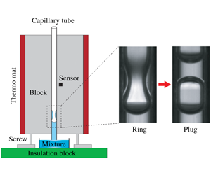
Figure 1. Solutal Marangoni effect in capillary tubes. (a) Schematic of the experimental set-up. The temperature of the Al blocks is controlled by employing two thermo mats, a sensor and a control unit (see appendix A). (b) Flow morphologies obtained with an ethanol/water mixture [40 % ( $v/v$)]: at a comparatively low temperature, we first observe thin climbing films inside the tube (see supplementary movie 1, available online at https://doi.org/10.1017/jfm.2020.80,
  $T_{con}=85\,^{\circ }\text{C}$). After a while, liquid accumulates, producing a thicker film with perturbations, a part of which has the shape of rings (see supplementary movie 2,
  $T_{con}=85\,^{\circ }\text{C}$). Upon further increase of the temperature (see supplementary movie 3,
  $T_{con}=87.5\,^{\circ }\text{C}$), a liquid plug is formed from a ring-shaped perturbation. The diameter of the capillary tube is
  $d=1.0~\text{mm}$. (c) For a capillary tube with a diameter
  $d=0.7~\text{mm}$ and at a temperature
  $T_{con}=96\,^{\circ }\text{C}$, we observe multiple liquid rings and plugs (see supplementary movies 4 and 5).
2.2 Experimental observations
For all of the capillary tubes considered in this study ( $d=0.7~\text{mm}$ to
  $d=1.5~\text{mm}$), upon increasing
  $T_{con}$, we observe three different liquid morphologies: films, rings and plugs, as shown in figure 1(b). We illustrate these morphologies with experiments conducted with a tube of diameter
  $d=1.0~\text{mm}$. After the Al blocks arrive at a stable temperature,
  $T_{con}=85\,^{\circ }\text{C}$, we wait another 5 min, after which ethanol/water mixture is filled into the Petri dish up to a level where it touches the bottom of the capillary tube. Immediately, a liquid column with a concave meniscus is created in the capillary tube and rises to a certain height (compatible with Jurin’s law (de Gennes, Brochard-Wyart & Quéré Reference de Gennes, Brochard-Wyart and Quéré2004)), with vapour above the meniscus. Then, a thin film climbing the tube walls forms (see supplementary movie 1). Considering the uniform temperature distribution in the Al blocks (see appendix B, figure 13), we mainly attribute the spreading of the film to the solutal Marangoni effect due to the faster evaporation of ethanol from the mixture (Bekki et al. Reference Bekki, Vignes-Adler, Nakache and Adler1990). This is corroborated by control experiments with pure water or ethanol in which neither film spreading nor liquid ring formation is observed. The film spreading continues until gravity starts to become dominant, which results in the formation of an annular liquid ring with an inner diameter
  $d_{l}$ inside the capillary (see supplementary movie 2). Upon increasing the temperature to
  $T_{con}=87.5\,^{\circ }\text{C}$, the rings become so pronounced that they collapse to form plugs (see supplementary movie 3). The continuous increase of the ring volume is possible only when the liquid supply from the column overcomes the evaporation of liquid. After a plug has been formed, it is pushed upwards by the enclosed vapour, while the bottom meniscus is pushed downwards. In figure 15 of appendix B, the temperature ranges in which plug formation occurs are displayed. Film formation starts at temperatures approximately
  $2.5{-}5\,^{\circ }\text{C}$ below the lower boundary of these regions. When the temperature is too high (i.e. typically
  $T_{con}>107.5\,^{\circ }\text{C}$), none of these three liquid morphologies is observed. At such high temperatures, the liquid evaporates faster than the time needed for film formation. Studying/explaining these complex flow phenomena in their entirety is a challenging and extensive task going beyond the scope of this paper. Instead, we limit our focus to the study of liquid plug formation from liquid rings.
3 Modelling the quasi-static behaviour
The growth of the liquid ring is modelled as a quasi-static process based on the following statements: (1) small Weber and capillary numbers; (2) negligible Marangoni stresses compared to normal stresses along the surface of the liquid ring; (3) a negligible influence of gravity, which is characterized based on the capillary length  $l_{c}=(\unicode[STIX]{x1D70E}/\unicode[STIX]{x1D70C}g)^{1/2}\approx 2.72~\text{mm}$, in which the density
  $\unicode[STIX]{x1D70C}=997.1~\text{kg}~\text{m}^{-3}$ and surface tension
  $\unicode[STIX]{x1D70E}=72.15~\text{mN}~\text{m}^{-1}$ of water at
  $25\,^{\circ }\text{C}$ were used. Here,
  $g=9.81~\text{m}~\text{s}^{-2}$ is the gravitational acceleration.

Figure 2. Dependence of the instantaneous  $d_{l}$ on the time variable
  $(t_{0}-t)$, denoting
  $t_{0}$ the moment when
  $d_{l}=0$. The inner diameter of the capillary tube is
  $d=0.7~\text{mm}$, and the experiment was carried out at
  $T_{con}=92.5\,^{\circ }\text{C}$. The frames at the top show the time evolution of the liquid ring. The arrow (top right corner) indicates the direction in which time increases.
Before presenting the theoretical analysis, as an example, we first show the time evolution of  $d_{l}$ on a comparatively long time scale (
 ${\sim}1~\text{s}$) in the capillary tube with
  $d=0.7~\text{mm}$ at
  $92.5\,^{\circ }\text{C}$ (see figure 2). This time span is much longer than the capillary time
  $t^{\ast }=[\unicode[STIX]{x1D70C}(d/2)^{3}/\unicode[STIX]{x1D70E}]^{1/2}\approx 0.77~\text{ms}$. The typical values of the Weber number and the capillary number in our experiments are estimated, respectively, as
  $We=\unicode[STIX]{x1D70C}u^{2}d/\unicode[STIX]{x1D70E}\approx 1.19\times 10^{-6}\ll 1$ and
  $Ca=\unicode[STIX]{x1D702}u/\unicode[STIX]{x1D70E}\approx 4.32\times 10^{-6}\ll 1$, in which
  $u=\text{d}(d/2)/\text{d}t\approx 0.35~\text{mm}~\text{s}^{-1}$ is the velocity with which the radius of the liquid ring changes,
  $\unicode[STIX]{x1D702}=0.891~\text{mPa}~\text{s}$ is the viscosity of water at
  $25\,^{\circ }\text{C}$. This analysis suggests that during the growth of the liquid ring up to the point where it becomes unstable, the roles of the inertia and viscosity of the liquid can be ignored, and the surface tension is dominant. Therefore, the liquid ring can be characterized by a static wetting state.
It has to be mentioned that statement 2 above is an assumption rather than an established fact. Based on the temperature uniformity at the surface of the capillary tube it can be shown that the thermal Marangoni stress can be neglected compared to the normal stress, but the significance of the solutal Marangoni stress cannot be excluded a priori.
Under these assumptions, the profile of the liquid surface is controlled by the Young–Laplace equation  $\unicode[STIX]{x0394}P=-2H\unicode[STIX]{x1D70E}$, denoting
  $\unicode[STIX]{x0394}P$ the pressure difference between the liquid and the vapour phase and
  $2H$ the total surface curvature. Based on that, we determined an exact analytical solution for the profile of the liquid surface.
3.1 Static profile of the liquid surface

Figure 3. (a) Example of a liquid ring observed in the experiments. (b) Schematic map for the modelling of the liquid in a capillary tube using an axisymmetric coordinate system. Here  $r=d/2$ and
  $r_{l}=d_{l}/2$ denote the inner radii of the capillary tube and the liquid ring, respectively;
  $h_{l}$ denotes the height of the solid–liquid contact region with a contact angle
  $\unicode[STIX]{x1D703}=0^{\circ }$;
  $s$ represents the arc length of the surface profile, starting from an arbitrary point
  $(x,z)$ of the surface; and
  $\unicode[STIX]{x1D719}$ is the angle of the normal vector of the surface at
  $(x,z)$ with the axis of revolution (i.e. the
  $z$-axis).
Inspired by the pioneering work of Carroll (Reference Carroll1976), we will derive analytical solutions for the liquid surface profile in the capillary tube. Here, we ignore gravity and set the value of the contact angle  $\unicode[STIX]{x1D703}=0^{\circ }$, corresponding to the experimental value. On the basis of differential geometry (Struik Reference Struik1961), the curvature
  $2H$ of the liquid–vapour interface can be expressed as
 $$\begin{eqnarray}2H=\frac{\sin \unicode[STIX]{x1D719}}{x}+\frac{\text{d}\unicode[STIX]{x1D719}}{\text{d}s},\end{eqnarray}$$
where the required geometrical parameters are defined in figure 3(b). We obtain the following relationships:
 $$\begin{eqnarray}\displaystyle & \displaystyle \frac{\text{d}z}{\text{d}x}=\frac{x^{2}+r\cdot r_{l}}{[(x^{2}-x_{l}^{2})(r^{2}-x^{2})]^{1/2}}, & \displaystyle\end{eqnarray}$$
 $$\begin{eqnarray}\displaystyle & \displaystyle 2H=\frac{2}{r+r_{l}}. & \displaystyle\end{eqnarray}$$
 Obviously, for a specific liquid profile (or  $r_{l}$),
  $H$ is constant globally. We employ the following transformation (Carroll Reference Carroll1976):
 $$\begin{eqnarray}x^{2}=r^{2}(1-k^{2}\sin ^{2}\unicode[STIX]{x1D711}),\end{eqnarray}$$
 in which  $k^{2}=1-(r_{l}/r)^{2}$. We write the boundary conditions as: (i)
  $x_{1}=r$,
  $z_{1}=h_{l}/2$,
  $\unicode[STIX]{x1D719}_{1}=\unicode[STIX]{x03C0}/2$,
  $\unicode[STIX]{x1D711}_{1}=0$; (ii)
  $x_{2}=r_{l}$,
  $z_{2}=0$,
  $\unicode[STIX]{x1D719}_{2}=\unicode[STIX]{x03C0}/2$,
  $\unicode[STIX]{x1D711}_{2}=\unicode[STIX]{x03C0}/2$. Inserting (3.4) into (3.2) and carrying out the integrals, we finally obtain
 $$\begin{eqnarray}z=\pm [r\cdot E(\unicode[STIX]{x1D711},k)+r_{l}\cdot F(\unicode[STIX]{x1D711},k)],\quad \unicode[STIX]{x1D711}\in [0,\unicode[STIX]{x03C0}/2],\end{eqnarray}$$
and
 $$\begin{eqnarray}\displaystyle & \displaystyle h_{l}=2[r\cdot E(k)+r_{l}\cdot K(k)], & \displaystyle\end{eqnarray}$$
 $$\begin{eqnarray}\displaystyle & \displaystyle A_{sl}=4\unicode[STIX]{x03C0}r[r\cdot E(k)+r_{l}\cdot K(k)], & \displaystyle\end{eqnarray}$$
 $$\begin{eqnarray}\displaystyle & \displaystyle A_{lv}=4\unicode[STIX]{x03C0}r(r+r_{l})E(k), & \displaystyle\end{eqnarray}$$
 $$\begin{eqnarray}\displaystyle & \displaystyle \frac{U}{4\unicode[STIX]{x03C0}\unicode[STIX]{x1D70E}}=r\cdot r_{l}[E(k)-K(k)], & \displaystyle\end{eqnarray}$$
 $$\begin{eqnarray}\displaystyle V_{l} & = & \displaystyle 2\unicode[STIX]{x03C0}r^{2}[r\cdot E(k)+r_{l}\cdot K(k)]-\frac{2\unicode[STIX]{x03C0}}{3}r_{l}^{3}\left(\frac{r}{r_{l}}\right)\nonumber\\ \displaystyle & & \displaystyle \times \left\{\left[2\left(\frac{r}{r_{l}}\right)^{2}+3\left(\frac{r}{r_{l}}\right)+2\right]E(k)-K(k)\right\},\end{eqnarray}$$
 in which  $A_{sl}$ and
  $A_{lv}$ are the solid–liquid and liquid–vapour interfacial areas;
  $h_{l}$ is the vertical height of
  $A_{sl}$;
  $U$ is a surface energy and defined by
  $U=\unicode[STIX]{x1D70E}(A_{lv}-A_{sl}\cos \unicode[STIX]{x1D703})$;
  $V_{l}$ is the volume of the liquid enclosed by the solid–liquid and liquid–vapour interfaces;
  $F(\unicode[STIX]{x1D711},k)$ and
  $E(\unicode[STIX]{x1D711},k)$ are the incomplete elliptic integrals of the first and the second kind, and
  $K(k)$ and
  $E(k)$ are the complete elliptic integrals of the first and the second kind (Magnus, Oberhettinger & Soni Reference Magnus, Oberhettinger and Soni1966), respectively. Based on the above results, we can not only derive the relationships between
  $d_{l}$ and
  $V_{l}$ as well as between
  $d_{l}$ and
  $U$ (see figure 4), we can also compute the surface profile of the liquid ring for different values of
  $d_{l}$ (as presented in figure 5 in dimensionless form).

Figure 4. Dependence of the volume  $V_{l}$ (left-hand side) and the surface energy
  $U$ (right-hand side) on the diameter of the liquid throat
  $d_{l}$, displayed in a dimensionless manner. The red solid and blue dashed lines represent the stable and unstable regimes, respectively. Points A and B are configurations with the same
  $V_{l}$ but different
  $d_{l}$ and
  $U$. The profiles in the inset on the left-hand side are the model results corresponding to the configurations A (red solid curve) and B (blue dashed curve). The inset on the right-hand side corresponds to
  $d_{l}/d\approx d_{lc}/d=0.417$. The contact angle is
  $\unicode[STIX]{x1D703}=0^{\circ }$.
Figure 4 shows the dependence of the volume of the liquid ring and its total surface energy derived from the Young–Laplace equation on  $d_{l}/d$. Interestingly, figure 4 represents a multiple solution map of the surface profile. As an example, a given liquid volume
  $V_{l}/(d/2)^{3}\approx 3.85$ corresponds to two different surface profiles which are plotted in the inset of figure 4 (left-hand side). These two profiles correspond to
  $d_{lA}/d\approx 0.74$ (point A) and
  $d_{lB}/d\approx 0.1$ (point B), respectively. However, the right-hand side of figure 4 suggests that the dimensionless surface energy of the profile corresponding to A (
 $U_{A}/[(d/2)^{2}\unicode[STIX]{x1D70E}]\approx -4.09$) is lower than that of the other one (
 $U_{B}/[(d/2)^{2}\unicode[STIX]{x1D70E}]\approx -3.37$). This means that under a perturbation, configuration B can transform into A, which is the only one found in the experiments. Figure 4 also shows that a liquid ring has a maximum volume,
  $V_{lc}$, corresponding to a minimum throat diameter,
  $d_{lc}$. Based on the minimum-volume theorem formulated by Langbein (Reference Langbein2002), the point
  $(V_{lc},d_{lc})$ corresponds to a point of instability. This means that upon further increase of the volume, a liquid ring does not exist as an equilibrium solution. The growth of a ring starts at zero volume, which means that we obtain the configuration indicated by the red line in figure 4. The ring continues to grow until the maximum volume is reached. This marks the transition to a liquid plug (see supplementary movie 3). The critical parameters related to this morphology transition can be determined rigorously based on the analytical model below.
3.2 Critical parameters for the morphology transition
Next, we determine the maximum volume of the liquid ring as shown in figure 4. This value is found by solving  $\unicode[STIX]{x2202}V_{l}/\unicode[STIX]{x2202}r_{l}=0$. For the sake of simplicity, we redefine
 $$\begin{eqnarray}\bar{V}_{l}=\frac{V_{l}}{2\unicode[STIX]{x03C0}r^{3}}=E(k)+\bar{r}_{l}K(k)-\frac{1}{3}[(2+3\bar{r}_{l}+2\bar{r}_{l}^{2})E(k)-\bar{r}_{l}^{2}K(k)],\end{eqnarray}$$
 in which  $\bar{r}_{l}=r_{l}/r=d_{l}/d$,
  $k=(1-\bar{r}_{l}^{2})^{1/2}$. Finally, we obtain
 $$\begin{eqnarray}\frac{\unicode[STIX]{x2202}\bar{V}_{l}}{\unicode[STIX]{x2202}\bar{r}_{l}}=(1+\bar{r}_{l})K(k)-2(1+\bar{r}_{l})E(k).\end{eqnarray}$$
The maximum volume of the liquid ring is then obtained from
 $$\begin{eqnarray}2E(k)-K(k)=0.\end{eqnarray}$$
The redefinition
 $$\begin{eqnarray}\bar{U}=\frac{U}{4\unicode[STIX]{x03C0}r^{2}\unicode[STIX]{x1D70E}}=\bar{r}_{l}[E(k)-K(k)]\end{eqnarray}$$
yields
 $$\begin{eqnarray}\frac{\unicode[STIX]{x2202}\bar{U}}{\unicode[STIX]{x2202}\bar{r}_{l}}=2E(k)-K(k).\end{eqnarray}$$
 Therefore,  $\unicode[STIX]{x2202}\bar{U}/\unicode[STIX]{x2202}\bar{r}_{l}=0$ also leads to (3.13). These analyses indicate that a maximum volume of the liquid corresponds to a minimum surface energy (see figure 4). Equation (3.13) is solved numerically to yield
 $$\begin{eqnarray}k=0.909,\quad \frac{d_{lc}}{d}=0.417.\end{eqnarray}$$
A combination of (3.16) and (3.3), (3.6), (3.9) and (3.10) finally leads to
 $$\begin{eqnarray}\displaystyle \left.\begin{array}{@{}c@{}}\displaystyle 2H_{c}\cdot \left(\frac{d}{2}\right)=1.411,\quad \frac{h_{lc}}{(d/2)}=4.257,\\ \displaystyle \frac{U_{c}}{(d/2)^{2}\unicode[STIX]{x1D70E}}=-6.081,\quad \frac{V_{lc}}{(d/2)^{3}}=5.471,\end{array}\right\} & & \displaystyle\end{eqnarray}$$
 denoting  $d_{lc}$,
  $h_{lc}$,
  $H_{c}$,
  $U_{c}$,
  $V_{lc}$ the values of
  $d_{l}$,
  $h_{l}$,
  $H$,
$H$,  $U$,
$U$,  $V_{l}$ at the transition point. The critical volume obtained in (3.17) is exactly equal to the value obtained by Everett & Haynes (Reference Everett and Haynes1972). Moreover, the critical diameter and the critical volume in (3.16) and (3.17), respectively, are consistent with the values obtained by Gauglitz & Radke (Reference Gauglitz and Radke1988) who solved an approximate form of the Young–Laplace equation using numerical methods. Extending the above analysis to contact angles different from zero (Lv & Hardt Reference Lv and Hardt2019) means that as long as the liquid surface exhibits a spatially uniform surface tension, the dimensionless values of these critical parameters are solely functions of the contact angle
  $\unicode[STIX]{x1D703}$.
3.3 Comparison between experimental and model results
Figure 5 shows a comparison between the experimentally observed surface profiles of the liquid rings and the analytical solution for different values of  $d_{l}/d$. The two data sets agree reasonably well. Strictly, when comparing experimental images of the interior of the tube with theoretical predictions, light refraction at the glass–air and glass–liquid interfaces needs to be taken into account. In other words, due to the curved interfaces, objects inside the tube usually appear distorted. However, based on a ray-tracing calculation, it can be shown that the distortion vanishes when imaging the gas–liquid interface itself. Therefore, it is justified to use the raw experimental data in figure 5. For even smaller values of
  $d_{l}/d$ (i.e.
  $d_{l}/d<0.417$), the liquid rings become unstable, and a quasi-static configuration can no longer be found. Instead, the hole closes rapidly.

Figure 5. Comparison between theoretical (red solid lines) and experimental surface shapes for different values of  $d_{l}/d$. The arrow represents the lapse of time. A tube with an inner diameter
  $d=1.5~\text{mm}$ was chosen, at
  $T_{con}=92.5\,^{\circ }\text{C}$.
In order to verify the model predictions in § 3.2, we carried out systematic tests using capillary tubes with four different inner diameters at different temperatures (see appendix A, table 2). We note that after  $d_{l}$ has reached
  $d_{lc}$, the growth of the liquid ring and the corresponding morphology transition to a plug happens very fast (characterized by the capillary time, i.e.
  ${\sim}1~\text{ms}$, see supplementary movie 3). In this case, it is reasonable to assume that the volume of the liquid ring remains constant during the transition event. This volume conservation provides an effective way to verify (3.16) using the simple relationship
  $\unicode[STIX]{x03C0}(d/2)^{2}(h+d)-\unicode[STIX]{x03C0}d^{3}/6=V_{lc}$, which leads to
 $$\begin{eqnarray}\frac{h}{d}=0.537,\end{eqnarray}$$
 in which  $h$ denotes the final thickness of the liquid plug. Its value can be accurately measured from high-speed images immediately after plug formation (see supplementary movie 3). The axial length (i.e. along
  $z$-axis, see figure 3) of the liquid plug immediately following closure predicted in (3.18) is exactly equal to the value obtained by Everett & Haynes (Reference Everett and Haynes1972). In figure 6, we see that the prediction of (3.18) is very close to the experimental results.

Figure 6. Dependence of  $h/d$ on
  $T_{con}$ for the transition from a liquid ring to a plug. For each
  $d$, the corresponding symbols cover the temperature range in which plugs are produced (see appendix B, figure 15). Each point is the average value of five individual measurements with the standard deviation shown as error bars. The inset illustrates the two different liquid morphologies. The red dashed line is the prediction of (3.18).
We have also analysed the vertical distance  $L$ between the position where the plug forms and the liquid meniscus at the bottom. Experiments were carried out using the same four capillary tubes within the same temperature range as in figure 6. Figure 7 shows that the value
  $L/d$ tends to increase with
  $T_{con}$. This makes sense intuitively: a higher temperature gives rise to a higher evaporation rate, and we hypothesize that the gas flow may lift the liquid rings. However, at present we are not able to measure or compute the gas flow rate to confirm this hypothesis. Even though the data points are quite scattered, it is striking that the diagram suggests that a minimum value of
  $L/d$ exists. This minimum value can be explained along the following line of thought: if we assume that the lower boundary of the annular liquid ring touches the liquid–vapour meniscus at the bottom (see supplementary movie 3), we obtain a quantitative prediction of the minimum value of
  $L$, i.e.
  $L_{c}=h_{lc}/2+d/2$. Since
  $h_{lc}/d$ is known from (3.17), we obtain
 $$\begin{eqnarray}\frac{L_{c}}{d}=1.564,\end{eqnarray}$$
which reproduces the lower bound of the experimental data of figure 7 quite well.

Figure 7. Dependence of  $L/d$ on
  $T_{con}$ for the transition from a liquid ring to a plug. For each
  $d$, the corresponding symbols cover the temperature range in which plugs are produced (see appendix B, figure 15). There are at least five individual measurements reported for each tube at each temperature. The red dashed lines are the prediction of (3.19).
4 Dynamic evolution of the liquid surface
4.1 Dynamics of liquid ring collapse
To explore the dynamics of the transition from liquid rings to plugs, a high-speed camera at 100 000 frames per second (f.p.s) with a resolution of  $4~\unicode[STIX]{x03BC}\text{m}~\text{pixel}^{-1}$ was employed. Experiments were carried out at
  $T_{con}=92.5\,^{\circ }\text{C}$, and the corresponding images are shown in the inset of figure 8. An analysis of the high-speed videos reveals the relationship
  $d_{l}/d\approx (0.77\pm 0.05)[(t_{0}-t)/t^{\ast }]^{0.57\pm 0.02}$ for the final stages of liquid ring collapse, in which
  $t_{0}$ is the moment when
  $d_{l}=0$,
  $t^{\ast }=[\unicode[STIX]{x1D70C}(d/2)^{3}/\unicode[STIX]{x1D70E}]^{1/2}$ is the characteristic time, and the prefactor was determined through fitting to the data points. Since it is very challenging to measure the values of the relevant material properties locally inside the capillary tube, for convenience we use the properties of pure water at
  $25\,^{\circ }\text{C}$ (i.e.
  $\unicode[STIX]{x1D70E}=72.15~\text{mN}~\text{m}^{-1}$ and
  $\unicode[STIX]{x1D70C}=997.1~\text{kg}~\text{m}^{-3}$) to determine
  $t^{\ast }$. We point out that the use of different liquid properties (for example, those of the 40 % (
 $v/v$) ethanol/water mixture) would result in different values of
  $t^{\ast }$ and the following scaling relationships of this section. However, the maximum property variation that may occur in the experiments limits the variation of the coefficients in all scaling relationships to less than a factor of 2, with one exception to be discussed later.
In fact, the collapse of the liquid ring in our experiments is reminiscent of the final stages of the pinch-off of air bubbles in an inviscid liquid, which has been investigated extensively in the past. Longuet-Higgins, Kerman & Lunde (Reference Longuet-Higgins, Kerman and Lunde1991) demonstrated that the evolution approximately follows a power law  $d_{l}\sim t^{0.5}$, which is supported by similar works (Oguz & Prosperetti Reference Oguz and Prosperetti1993; Burton, Waldrep & Taborek Reference Burton, Waldrep and Taborek2005). Thoroddsen, Etoh & Takehara (Reference Thoroddsen, Etoh and Takehara2007) investigated the pinch-off of a bubble in water and found that the shrinking of the neck of the bubbles obeys
  $d_{l}\sim t^{0.57\pm 0.03}$, which is in good agreement with the numerical work carried out by Leppinen & Lister (Reference Leppinen and Lister2005) who studied the breakup of a bubble in an inviscid liquid and obtained
  $d_{l}\sim t^{0.55\pm 0.01}$. From a theoretical and numerical point of view, Gordillo et al. (Reference Gordillo, Sevilla, Rodríguez-Rodríguez and Martinez-Bazan2005) and Eggers et al. (Reference Eggers, Fontelos, Leppinen and Snoeijer2007) studied the collapse of an axisymmetric cavity in a low-viscosity fluid. By ignoring the influences of surface tension, gas density and viscosity, they obtained the relationship
  $d\sim t^{\unicode[STIX]{x1D6FC}}$, with time-dependent scaling exponents
  $\unicode[STIX]{x1D6FC}\approx 1/2+1/[-4\ln (t_{0}-t)]$ and
  $\unicode[STIX]{x1D6FC}\approx 1/2+1/[4\sqrt{-\ln (t_{0}-t)}]$, respectively. The scaling relation put forward by Eggers et al. (Reference Eggers, Fontelos, Leppinen and Snoeijer2007) was further verified by Gekle et al. (Reference Gekle, Snoeijer, Lohse and Meer2009) who studied the pinch-off of air bubbles surrounded by an inviscid fluid in four different systems. Eggers et al. (Reference Eggers, Fontelos, Leppinen and Snoeijer2007) further obtained a small decrease of the scaling exponent from 0.57 to 0.55 (corresponding to the pinch-off) during the collapse, which indicates that the dynamics of inviscid bubble pinch-off is not universal. Our results are consistent with the theoretical prediction by Eggers et al. (Reference Eggers, Fontelos, Leppinen and Snoeijer2007), indicating that viscosity and the presence of air inside the liquid ring can be neglected, and that capillary forces only trigger the instability.

Figure 8. Normalized instantaneous inner diameter of a collapsing liquid ring as a function of the normalized time  $(t_{0}-t)/t^{\ast }$. Each data point is the average value of five individual measurements with the standard deviation shown as error bars. The black solid line represents
  $d_{l}\sim (t_{0}-t)^{0.57\pm 0.02}$. The frames in the inset (the black region with white reflections indicates vapour, the grey region liquid) corresponds to times
  $(t_{0}-t)\approx 3.7~\text{ms},3.5~\text{ms},2.5~\text{ms},0~\text{ms}$, and the scale bar represents
  $200~\unicode[STIX]{x03BC}\text{m}$.
4.2 Dynamics of liquid plug formation
After the hole of the liquid ring has closed, a growing liquid column is formed that finally evolves into a plug, as shown in figure 9 and the inset of figure 12. This closing process bears some similarities to the coalescence of liquid drops or air bubbles (Ristenpart et al. Reference Ristenpart, McCalla, Roy and Stone2006; Paulsen et al. Reference Paulsen, Carmigniani, Kannan, Burton and Nagel2014; Eddi, Winkels & Snoeijer Reference Eddi, Winkels and Snoeijer2013; Thoroddsen et al. Reference Thoroddsen, Etoh, Takehara and Ootsuka2005; Bird et al. Reference Bird, Ristenpart, Belmonte and Stone2009; de Maleprade, Clanet & Quéré Reference de Maleprade, Clanet and Quéré2016), which has been studied quite intensely. Previous results (Eggers, Lister & Stone Reference Eggers, Lister and Stone1999) suggest that a one-dimensional model can already capture the essential physics. As shown in the inset of figure 9, we denote  $\unicode[STIX]{x1D6FF}$ the characteristic width of the liquid column,
  $\unicode[STIX]{x1D705}$ the curvature computed from the minor radius of the liquid ring, and
  $X$ the time-dependent height of the liquid column. In an order-of-magnitude sense, we have
  $1/\unicode[STIX]{x1D705}\sim d/2$. From the geometric configuration depicted in the inset of figure 9, we obtain the scaling relationship
  $X^{2}\sim \unicode[STIX]{x1D6FF}d/2$ if
  $\unicode[STIX]{x1D6FF}\ll d$. Hence, the balance between the capillary and the inertial force leads to
  $\unicode[STIX]{x1D70E}/\unicode[STIX]{x1D6FF}\sim \unicode[STIX]{x1D70C}[X/(t-t_{0})]^{2}$, which finally produces a scaling relationship
  $X\sim [\unicode[STIX]{x1D70E}(d/2)/\unicode[STIX]{x1D70C}]^{1/4}(t-t_{0})^{1/2}$. Determining the prefactor in this relationship by fitting the experimental data gives
 $$\begin{eqnarray}\frac{X}{d}\approx (1.0\pm 0.03)\left(\frac{t-t_{0}}{t^{\ast }}\right)^{0.5\pm 0.01}.\end{eqnarray}$$
Figure 9. Dependence of the normalized instantaneous liquid column height  $X/d$ on the normalized time
  $(t-t_{0})/t^{\ast }$ in log–log plot. Each point is the average value of five individual measurements with the standard deviation indicated as error bars. The black solid line is computed from (4.1). The schematic illustrates the geometry used for the scaling analysis. The high-speed image shows the liquid surface profile shortly before closure (the black region is vapour and the grey region is liquid), the scale bar represents
  $50~\unicode[STIX]{x03BC}\text{m}$ (see supplementary movies 6 and 7).
4.3 Oscillation of the liquid plug
After the formation of a plug, shape oscillations can be observed (see supplementary movie 7). These oscillations can be described by combining the concept of a damped harmonic oscillator with a scaling analysis, which we will present in this section.
The differential equation of a damped harmonic oscillator is given by
 $$\begin{eqnarray}m\ddot{X}+b{\dot{X}}+kX=0,\end{eqnarray}$$
 in which  $X=X(t)$ is the instantaneous thickness of the liquid plug,
  $m$ is its mass,
  $b$ is the damping coefficient, and
  $k$ is the spring constant. The general solution of (4.2) is
 $$\begin{eqnarray}\displaystyle X(t) & = & \displaystyle X_{0}+X_{1}\exp (-\unicode[STIX]{x1D709}\unicode[STIX]{x1D714}_{n}t)\sin (\unicode[STIX]{x1D714}_{d}+\unicode[STIX]{x1D711})\nonumber\\ \displaystyle & = & \displaystyle X_{0}+X_{1}\exp (-\unicode[STIX]{x1D6FD}t)\sin \left(2\unicode[STIX]{x03C0}\frac{t}{T}+\unicode[STIX]{x1D711}\right),\end{eqnarray}$$
 in which  $X_{0}$ denotes the thickness of the liquid plug after the oscillation has disappeared, i.e.
  $X_{0}=X|_{t\rightarrow \infty }=h$. The amplitude
  $X_{1}$ and phase
  $\unicode[STIX]{x1D711}$ have to be determined from the initial conditions. Furthermore, we use the following abbreviations/relationships:
 $$\begin{eqnarray}\displaystyle \unicode[STIX]{x1D6FD}=\unicode[STIX]{x1D709}\unicode[STIX]{x1D714}_{n},\quad \unicode[STIX]{x1D714}_{n}=\sqrt{\frac{k}{m}},\quad \unicode[STIX]{x1D709}=\left(\frac{b}{m}\right)\frac{1}{2\unicode[STIX]{x1D714}_{n}}, & & \displaystyle\end{eqnarray}$$
 $$\begin{eqnarray}\displaystyle & \displaystyle \unicode[STIX]{x1D714}_{d}=\frac{2\unicode[STIX]{x03C0}}{T}=\sqrt{1-\unicode[STIX]{x1D709}^{2}}\cdot \unicode[STIX]{x1D714}_{n}=\sqrt{\unicode[STIX]{x1D714}_{n}^{2}-\unicode[STIX]{x1D6FD}^{2}}=\sqrt{1-\frac{1}{4}\frac{b^{2}}{mk}}\cdot \sqrt{\frac{k}{m}}, & \displaystyle\end{eqnarray}$$
 $$\begin{eqnarray}\displaystyle & \displaystyle T=\frac{2\unicode[STIX]{x03C0}}{\sqrt{1-\displaystyle \frac{1}{4}\frac{b^{2}}{mk}}\cdot \sqrt{\displaystyle \frac{k}{m}}}. & \displaystyle\end{eqnarray}$$
 We can identify the orders of magnitude of the unknown parameters (i.e.  $m$,
$m$,  $b$ and
  $k$) by a scaling analysis:
 $$\begin{eqnarray}m\sim \unicode[STIX]{x1D70C}\left(\frac{d}{2}\right)^{3},\quad b\sim \unicode[STIX]{x1D702}\left(\frac{d}{2}\right),\quad k\sim \unicode[STIX]{x1D70E}.\end{eqnarray}$$
 Based on that, the influence of the damping coefficient on the oscillation period can be expressed by the Ohnesorge number  $Oh$:
$Oh$:
 $$\begin{eqnarray}\frac{b^{2}}{mk}\sim \frac{\unicode[STIX]{x1D702}^{2}}{\unicode[STIX]{x1D70C}\unicode[STIX]{x1D70E}(d/2)}=Oh^{2},\end{eqnarray}$$
 which relates the viscous forces to inertial and surface-tension forces, can be estimated as  $Oh\approx 4.70\times 10^{-3}$ (
 $d=1.0~\text{mm}$ is used). This indicates that the influence of viscous force on the oscillation period is weak. For the sake of simplicity, we assume
 $T=2\unicode[STIX]{x03C0}/\unicode[STIX]{x1D714}_{d}\approx 2\unicode[STIX]{x03C0}/\unicode[STIX]{x1D714}_{n}$.
4.4 Model parameter identification from experiments
In this section, we describe how the parameters of the harmonic oscillator model have been determined from the experimental data.
Finding  $X_{0}$
In the limit  $t\rightarrow \infty$, the thickness of the liquid plug reaches a constant value (i.e.
  $X|_{t\rightarrow \infty }=0.5374d$), which suggests
 $$\begin{eqnarray}X_{0}=0.5374\;d.\end{eqnarray}$$
 Equation (4.9) is based on a theoretical analysis.  $X_{0}$ can also be determined experimentally. We obtain
  $X_{0}/d=0.52\pm 0.01,0.51\pm 0.01,0.51\pm 0.01$ and
  $0.50\pm 0.02$ for capillary tubes with
  $d=0.7~\text{mm}$, 1.0 mm, 1.38 mm and 1.5 mm, respectively (see table 1), which is reasonably close to the theoretical results. The somewhat lower experimental values are probably due to evaporation of liquid.
Finding  $T$
$T$
Considering that the oscillation of the liquid results from the competition between inertia and surface tension, the oscillation period should scale as  $T\sim [\unicode[STIX]{x1D70C}(d/2)^{3}/\unicode[STIX]{x1D70E}]^{1/2}$. Let us define
 $$\begin{eqnarray}T=c_{1}t^{\ast }=c_{1}\left[\frac{\unicode[STIX]{x1D70C}}{\unicode[STIX]{x1D70E}}\left(\frac{d}{2}\right)^{3}\right]^{1/2},\end{eqnarray}$$
 in which  $t^{\ast }=[\unicode[STIX]{x1D70C}(d/2)^{3}/\unicode[STIX]{x1D70E}]^{1/2}$ is the characteristic time, and
  $c_{1}$ is a dimensionless coefficient. Since
  $T$ can be measured directly,
  $c_{1}$ can be determined.
Finding  $\unicode[STIX]{x1D6FD}$
Based on the above analysis (i.e. (4.3), (4.4) and (4.7)) we have
 $$\begin{eqnarray}\unicode[STIX]{x1D6FD}=\unicode[STIX]{x1D709}\unicode[STIX]{x1D714}_{n}=\frac{b}{2m}\sim \frac{\unicode[STIX]{x1D702}}{\unicode[STIX]{x1D70C}(d/2)^{2}}.\end{eqnarray}$$
 For convenience, using (4.8), we can rewrite  $\unicode[STIX]{x1D6FD}$ as
 $$\begin{eqnarray}\unicode[STIX]{x1D6FD}=c_{2}\frac{\unicode[STIX]{x1D702}}{\unicode[STIX]{x1D70C}(d/2)^{2}}=c_{2}\frac{1}{t^{\ast }}\cdot Oh,\end{eqnarray}$$
 in which  $c_{2}$ is a dimensionless coefficient. On the other hand,
 $$\begin{eqnarray}\unicode[STIX]{x1D6FD}=\unicode[STIX]{x1D709}\unicode[STIX]{x1D714}_{n},\quad \unicode[STIX]{x1D709}=\frac{\unicode[STIX]{x1D6E4}/2\unicode[STIX]{x03C0}}{\sqrt{1+(\unicode[STIX]{x1D6E4}/2\unicode[STIX]{x03C0})^{2}}},\quad \unicode[STIX]{x1D6E4}=\ln A_{1}-\ln A_{2}=\ln \left(\frac{A_{1}}{A_{2}}\right),\end{eqnarray}$$
 in which  $A_{1}$ and
  $A_{2}$ are the values of
  $X(t)$ at any two successive maxima. We choose
  $A_{1}=X|_{t=T/2}-X_{0}$ and
  $A_{2}=X|_{t=3T/2}-X_{0}$ (see figure 10a). Here
  $\unicode[STIX]{x1D714}_{n}$ is measured through
  $\unicode[STIX]{x1D714}_{n}=2\unicode[STIX]{x03C0}/T$, in which the first period
  $T$ is used. Combining (4.12) and (4.13) gives
  $c_{2}$.
Based on the above analysis, we can rewrite (4.3) as
 $$\begin{eqnarray}X(t)=X_{0}+X_{1}\exp \left(-c_{2}\cdot Oh\cdot \frac{t}{t^{\ast }}\right)\cdot \sin \left(\frac{2\unicode[STIX]{x03C0}}{c_{1}}\cdot \frac{t}{t^{\ast }}+\unicode[STIX]{x1D711}\right),\end{eqnarray}$$
or, in dimensionless form,
 $$\begin{eqnarray}\bar{X}(t)=\bar{X}_{0}+\bar{X}_{1}\exp (-c_{2}\cdot Oh\cdot \bar{t})\cdot \sin \left(\frac{2\unicode[STIX]{x03C0}}{c_{1}}\cdot \bar{t}+\unicode[STIX]{x1D711}\right),\end{eqnarray}$$
 in which  $\bar{X}(t)=X(t)/d$,
  $\bar{X}_{0}=X_{0}/d$,
  $\bar{X}_{1}=X_{1}/d$ and
  $\bar{t}=(t-t_{0})/t^{\ast }$.
Finding  $X_{1}$ and
  $\unicode[STIX]{x1D711}$
Up to now,  $X_{1}$ and
  $\unicode[STIX]{x1D711}$ are the last two unknown parameters to be determined. From (4.9), we know
  $\sin [2\unicode[STIX]{x03C0}t/(c_{1}t^{\ast })]=\sin (2\unicode[STIX]{x03C0}t/T+\unicode[STIX]{x1D711})$. Checking the first period of the experimental data, we find approximately
  $X(t=T/2)=X_{max}$ and
  $X(t=T)=X_{min}$ (see the inset of figure 10a), which suggests that
  $\unicode[STIX]{x1D711}\approx -\unicode[STIX]{x03C0}/2$, resulting in
  $X_{1}>0$ (alternatively,
  $\unicode[STIX]{x1D711}\approx \unicode[STIX]{x03C0}/2$, resulting in
  $X_{1}<0$). Finally, we assume that the experimental value (
 $X|_{t=T/2}-X|_{t=T}$) (e.g. figure 10a) is equal to the corresponding theoretical value, i.e.
  $X(t=T/2)-X(t=T)$ in (4.9). By this method, we can determine
  $X_{1}$ for each tube.
Table 1. Coefficients of the harmonic oscillator model obtained from experiments with four different tubes. Here we use  $\unicode[STIX]{x1D711}=-\unicode[STIX]{x03C0}/2$ for each capillary tube.

In table 1, the resulting coefficients related to experiments with four different tubes are listed. The results in table 1 have been obtained from individual experiments. Each value represents the average of five independent measurements, from which standard errors have been computed.

Figure 10. Time evolution of the liquid plug thickness as obtained from the experiments (symbols) and the model (lines). The inner diameters of the capillary tubes are: (a)  $d=0.7~\text{mm}$; (b)
  $d=1.0~\text{mm}$; (c)
  $d=1.38~\text{mm}$; and (d)
  $d=1.5~\text{mm}$. Each red dot is the average of five experiments, with error bars representing the standard deviation. The black solid lines are model results according to (4.14). All parameters are listed in table 2 in appendix A. The schematic in the inset of (b) depicts the geometrical parameters
  $A_{1}$,
  $A_{2}$ and
  $X_{0}$.
The comparisons shown in figure 10 suggest that our model (solid black lines) reproduces the experimental data (red dots) reasonably well. However, all the graphs show a deviation, especially in the first period. For a damped oscillator (see the inset of figure 10a), we should have  $(X|_{t=T/2}-X_{0})>(X_{0}-X|_{t=T})$; however, in the experiments we obtain
  $(X|_{t=T/2}-X_{0})<(X_{0}-X|_{t=T})$ for all capillary tubes. One possible reason is that after the liquid plug has been formed, gas is enclosed between the plug and the bottom meniscus, whereas the other side of the plug is open. This has the following consequences for the oscillation: (i) for
  $t\in [0,T/2]$,
  $X$ is increasing, meanwhile the gas is being compressed, which creates a force resisting the increase of
  $X$; (ii) on the contrary, for
  $t\in [T/2,T]$,
  $X$ is decreasing, meanwhile the gas is expanding, which promotes the increase of
  $X$. We have to emphasize that during the oscillation, we did not observe any appreciable downward motion of the bottom meniscus, which means the gas is indeed compressed.
The above analyses are for individual tubes only. Given that the physics represented by (4.14) is correct, it should be possible to formulate a uniformly valid model which allows the prediction of the plug oscillation in all different tubes. According to the model assumptions, the oscillation period should be proportional to  $t^{\ast }=[\unicode[STIX]{x1D70C}(d/2)^{3}/\unicode[STIX]{x1D70E}]^{1/2}$, while the damping coefficient should be proportional to
  $\unicode[STIX]{x1D702}/[\unicode[STIX]{x1D70C}(d/2)^{2}]$. Figure 11 compares the experimentally determined oscillation periods and damping coefficients for four different tubes with these scales. To a very good approximation, a direct proportionality between the experimentally determined values and the scales in the model holds true.

Figure 11. Relationship between (a)  $T$ and
  $t^{\ast }$; (b)
  $\unicode[STIX]{x1D6FD}$ and
  $\unicode[STIX]{x1D702}/[\unicode[STIX]{x1D70C}(d/2)^{2}]$. Here
  $T$ and
  $\unicode[STIX]{x1D6FD}$ are the measured values of the oscillation period and the damping factor. The red dashed lines are linear fits using the method of least squares. Each symbol is the average value of five experiments with standard errors.
By performing linear fits, we find  $c_{1}\approx 2.07$ and
  $c_{2}\approx 117.50$ based on (4.10) and (4.12).
  $X_{0}/d$ and
  $X_{1}/d$ are determined from table 1 by taking the average of the values corresponding to the four individual tubes. We obtain
  $X_{0}/d\approx 0.512$ (
 ${\sim}5\,\%$ deviation from the theory
  $X_{0}/d=0.537$) and
  $X_{1}/d\approx 0.15$. Therefore, on the basis of (4.15) the uniformly valid model is given as
 $$\begin{eqnarray}\bar{X}(t)=0.512+0.15\exp (-117.50\cdot Oh\cdot \bar{t})\cdot \sin \left(3.04\cdot \bar{t}-\frac{\unicode[STIX]{x03C0}}{2}\right).\end{eqnarray}$$
Comparisons between experimental data and (4.16) for four different capillary tubes are given in figure 12.

Figure 12. Dependence of the normalized instantaneous liquid column height  $x/d$ on the normalized time
  $(t-t_{0})/t^{\ast }$ in linear plot. Each point is the average value of five individual measurements with the standard deviation indicated as error bars. The solid lines are theoretical predictions of (4.16), with four colours corresponding to the experimental results in different tubes. The frames in the inset correspond to
  $(t-t_{0})\approx 0~\text{ms},0.1~\text{ms},0.25~\text{ms},0.6~\text{ms},1.3~\text{ms},2.8~\text{ms}$, and the scale bar represents
  $200~\unicode[STIX]{x03BC}\text{m}$.
The solid lines in figure 12 represent theoretical predictions for capillary tubes with different diameters. Equation (4.16) reproduces the experimental results reasonably well, but some deviations are visible. The only coefficient in all of the derived scaling relationships that strongly depends on the reference properties of the liquid is  $c_{2}$. It may vary by one order of magnitude if a different reference temperature of reference composition (within the scope of the experiments) is chosen. However, we wish to emphasize that the agreement between the experimental data points and the curves in figure 12 is unaffected by that.
5 Conclusions
In summary, we studied the evolution of the liquid surface in heated capillary tubes dipped into a bath filled with a binary mixture. Various morphologies, such as liquid films, rings and plugs, have been observed, as well as the transitions between them. Rings are formed in a similar way as the famous tears of wine by pulling up liquid through a thin film driven by solutal Marangoni stresses. A key phenomenon is the transition between a liquid ring and a plug. Based on the Young–Laplace equation, this can be understood as the collapse of a minimal surface beyond its stability threshold. Experimental and theoretical results for the stability threshold are in good agreement. Scaling laws describing the dynamics of the transition between liquid ring and plug as well as the oscillations of the plug after its formation have been identified. The observed phenomena could be relevant for a broad class of processes/phenomena in fields such as chemical engineering, microfluidics and geophysics. Future studies should be devoted to examining the complex dynamics occurring inside the tubes after the formation of single and especially multiple plugs.
Acknowledgements
The authors acknowledge the support by T. Homolla concerning the experimental set-up. C. L. would like to gratefully acknowledge the support from the Alexander von Humboldt Foundation of Germany, the National Natural Science Foundation of China (grant no. 11632009, 11872227), and Tsinghua University (grant no. 53330100319), Beijing, China. S. N. V. acknowledges funding from the Department of Science and Technology, INDIA (DST) through an INSPIRE faculty award (DST/INSPIRE/04/2015/000544). We are grateful to the anonymous reviewers whose suggestions have helped to significantly improve the paper.
Declaration of interests
The authors report no conflict of interest.
Supplementary movies
Supplementary movies are available at https://doi.org/10.1017/jfm.2020.80.
Appendix A. Materials and experimental methods
A.1 Sample preparation
Glass capillary tubes with different inner diameters are used in our experiments. First, the tubes are washed using ethanol and Milli-Q water, and then dried by clean compressed air. The key step is to treat the tubes with ‘piranha’ solution, which is composed of 70 % sulfuric acid solution ( $\text{H}_{2}\text{SO}_{4}$, 96 % in concentration) and 30 % hydrogen peroxide solution (
 $\text{H}_{2}\text{O}_{2}$, 30 % in concentration). On the one hand, the piranha solution removes potential contaminants; on the other hand, the strong oxidizing property of the solution renders the glass wall sufficiently hydrophilic, which is crucial for the experiments. The tubes are immersed in a glass container filled with piranha solution and heated to
  $90\,^{\circ }\text{C}$ for 30 min employing a hot plate. After that, they are cleaned using Milli-Q water and dried.
The relevant geometrical parameters (i.e. the inner and outer diameters  $d$ and
  $d_{out}$, wall thickness
  $\unicode[STIX]{x1D6E5}$ and length
  $l$) of the four types of capillary tubes are listed in table 2.
Table 2. Geometrical parameters of the capillary tubes used in the experiments, denoting $d$,
$d$,  $d_{out}$,
  $\unicode[STIX]{x1D6E5}$ and
  $l$ the inner and outer diameters, wall thickness and length, respectively.

A.2 Experimental set-up
The experimental set-up consists of a linear three-axis translation stage, two aluminum (Al) cuboids with dimensions of  $20\times 4\times 3~\text{cm}^{3}$ each, a high-speed camera (Photron Fastcam SA1.1 Model 675K-M1) attached to a long distance microscope, a strong light source (ZHONGFA, item no. 0203), two thermo mats (Silicon Rubber Heater, Rs-8607214), an insulation block (i.e. a wood block of
  $18\times 9\times 2~\text{cm}^{3}$), a temperature control unit (JUMO, LR 316), a temperature sensor (platinum resistance temperature sensor, Pt100) and a glass Petri dish (18.5 mm in diameter and 2.5 mm in height). Some key components of the experimental set-up are sketched in figure 1(a). The temperature sensor is attached to one Al block close to the capillary tube and linked to the control unit. The Petri dish contains the ethanol/water mixture [40 % (
 $v/v$)]. To provide a uniform illumination, a light diffuser panel arranged between the light source and the capillary tube is used. When neglecting the rays entering the capillary tube that are reflected from one of the metal surfaces, the corresponding illumination etendue is
  $33^{\circ }$. Ray-tracing calculations were performed showing that the imaging of the gas–liquid interface is not limited by the illumination etendue. The experiments were carried out on an optical table.
During the experiments, different recording speeds are employed. Low recording speeds guarantee a long time recording and a relatively large field of view (FOV), while high recording speeds are employed to capture the details of the dynamics during liquid plug formation. The highest recording speed used was 100 000 f.p.s with a resolution of  $4~\unicode[STIX]{x03BC}\text{m}~\text{pixel}^{-1}$.
Appendix B. Temperature measurements
The principle of temperature control in our system is as follows. The sensor (the black square as shown in figure 1a) fixed on the Al block is directly connected to the control unit, and the control unit and the two thermo mats are connected to each other. After a temperature has been set ( $T_{con}$, i.e. the target temperature) and the heating has started, the control unit monitors instantaneous temperature values (
 $T_{b}$) of the Al block. Via feedback control, the control unit not only lets
  $T_{b}$ approach
  $T_{con}$ in a sufficiently smooth process, but also restricts the fluctuations of
  $T_{b}$ to a very narrow band. Typical fluctuations are of the order of
  $\pm 0.2\,^{\circ }\text{C}$.

Figure 13. (a) Schematic diagram showing the points where the temperature has been measured after the target value  $T_{con}=95\,^{\circ }\text{C}$ has been reached. Ten points distributed uniformly along the Al block are chosen (
 ${\sim}3~\text{mm}$ from the inner boundary of each Al block). The Al blocks and the capillary tube are not to scale. (b) Table of measured temperatures. Here
  $T_{max}$ and
  $T_{min}$ are the maximum and minimum values of the temperature during a time span of 10 min,
  $T_{aver}=(T_{max}+T_{min})/2$ and
  $\unicode[STIX]{x0394}T=T_{max}-T_{min}$.
Since temperature gradients give rise to Marangoni stresses, a spatially uniform temperature in the Al blocks is very important. We measured the temperature at different points on the blocks. In this test,  $T_{con}$ was set to
  $95\,^{\circ }\text{C}$. As shown in figure 13, the ten corresponding points are close (
 ${\sim}3~\text{mm}$) to the edges of the Al blocks. At each point, the temperature sensor is attached using thermal paste, and the measurements started 10 min after the target temperature has been reached. The maximum (
 $T_{max}$) and minimum (
 $T_{min}$) values of
  $T_{b}$ during this 10 min period are tabulated in figure 13 (the right-hand side), which shows a fluctuation (
 $\unicode[STIX]{x0394}T=T_{max}-T_{min}$) of
  ${\sim}1\,^{\circ }\text{C}$. Moreover, the average value of the temperature of each point during this 10 min period, i.e.
  $T_{aver}=(T_{max}+T_{min})/2$, is given as well, which indicates temperature values
  $94.60\pm 0.18\,^{\circ }\text{C}$ and
  $94.85\pm 0.31\,^{\circ }\text{C}$ of the left and right blocks, respectively. Based on this, we conclude that a sufficiently uniform temperature distribution exists inside the blocks.
While a uniform temperature distribution in the Al blocks is important, the thermal resistances due to the capillary give rise to unavoidable non-uniformities. To quantify these non-uniformities, temperature values were taken with another three thermocouples (K type, 0.075 mm diameter of the probe tip) connected to a thermometer (Lutron TM-947SD), as shown in figure 14:
(i)
 $T_{in}$ (red circle): this thermocouple was put inside of the capillary tube, at a position slightly below the liquid–vapour meniscus;
(ii)
$T_{gw}$ (green upward pointing triangle): this thermocouple was mounted in such a way that it touches the outside wall of the tube;(iii)
$T_{mix}$ (blue downward pointing triangle): this thermocouple was placed in the bulk of the mixture in the container, ${\sim}7.5~\text{mm}$ away from the bottom of the capillary tube.


Figure 14. Schematic showing the four temperature measurement points, represented by a black square ( $T_{b}$), red circle (
 $T_{in}$), green upward pointing triangle (
 $T_{gw}$) and blue downward pointing triangle (
 $T_{mix}$).

Figure 15. Dependence of the temperature at four different positions ( $T_{b}$,
  $T_{in}$,
  $T_{gw}$,
  $T_{mix}$) on the target value (
 $T_{con}$) for four different capillary tubes. The black squares, red circles, green and blue triangles represent the values measured at the four different positions indicated in figure 14. Error bars are attached to all data points, but are too small to be visible in most cases. The tube diameters are: (a)
  $d=0.7~\text{mm}$; (b)
  $d=1.0~\text{mm}$; (c)
  $d=1.38~\text{mm}$; and (d)
  $d=1.5~\text{mm}$. The solid line (i.e.
  $T_{m}=T_{con}$) in each figure is used to guide the eye. The grey region in each figure indicates the range of
  $T_{con}$ in which liquid plugs are formed.
This test starts from room temperature and ends at a temperature of  ${\sim}107.5\,^{\circ }\text{C}$ (i.e. up to the point where liquid films can no longer be observed), based on the following protocol. First, a stable state is reached, meaning that
  $T_{b}$ reaches
  $T_{con}$. After a waiting time of 5 min, fresh mixture is filled into the Petri dish to a level where the liquid touches the capillary tube. Then, the recording of the temperature values at the four positions over a time span of 5 min starts. The corresponding maximum and minimum values over that time span are denoted by
  $T_{max}$ and
  $T_{min}$, respectively. In figure 15, the individual points represent the average values of
  $T_{max}$ and
  $T_{min}$, i.e.
  $(T_{max}+T_{min})/2$. Correspondingly, the error bar is defined as
  $\unicode[STIX]{x0394}T=(T_{max}-T_{min})/2$. Here
  $T_{m}$ denotes the measured values of
  $T_{b}$,
  $T_{in}$,
  $T_{gw}$ and
  $T_{mix}$, respectively. After this test, the Petri dish is removed, and the same procedure is performed again. Literature indicates that the boiling point of the mixture is approximately
  $83{-}84\,^{\circ }\text{C}$ (Reddy & Lienhard Reference Reddy and Lienhard1989). However, we did not observe any nucleate boiling within the considered temperature range.
When  $T_{con}\leqslant 85\,^{\circ }\text{C}$, climbing liquid films are hardly visible. As a consequence, no liquid rings or plugs are found. In this temperature regime,
  $T_{con}$ was increased in steps of
  $5\,^{\circ }\text{C}$. However, when
  $T_{con}\geqslant 85\,^{\circ }\text{C}$, the formation of films and other configurations sets in, so the step size was reduced to
  $2.5\,^{\circ }\text{C}$ to capture more details. Considering that evaporation always happens in the experiments, the composition of the ethanol/water mixture varies due to the different evaporation rates of water and ethanol. By employing a syringe, the mixture in the Petri dish was renewed frequently during these 5 min tests to guarantee a well-defined composition in the liquid reservoir.
Figure 15 shows that  $T_{b}$ always follows very well the target value;
  $T_{mix}$ is close to room temperature, but it slightly increases with
  $T_{con}$;
  $T_{in}$ is the key readout, because it indicates the temperature of the liquid mixture inside the tube. The grey region in each graph indicates in which range of
  $T_{con}$ liquid plugs are formed. Typically the grey regions range from
  $87.5\,^{\circ }\text{C}$ to
  $105\,^{\circ }\text{C}$ with an uncertainty of
  $\pm 1.25\,^{\circ }\text{C}$, corresponding to the left-hand and right-hand boundaries. The reasons for the uncertainty may be due to variations of the contact area with the Al block.
We aim at presenting a theoretical analysis of the profile of the liquid ring and the oscillation of the plug. In order to quantitatively analyse these phenomena, knowledge of the local liquid properties is required. It is very difficult to measure the relevant parameters, i.e. pressure, density, viscosity and surface tension, directly in the capillary tube. Although one could perform measurements in the bulk mixture, the boiling point of the mixture ( $83{-}84\,^{\circ }\text{C}$) (Reddy & Lienhard Reference Reddy and Lienhard1989) is lower than the upper limit of the temperature range (
 ${\sim}95\,^{\circ }\text{C}$, see figure 15) inside the capillary tube. Moreover, the relevant values of the material parameters vary due to dynamic temperature fluctuations. Therefore, in the theoretical analysis, for convenience we use the material properties of pure water at
  ${\sim}25\,^{\circ }\text{C}$ (i.e.
  $\unicode[STIX]{x1D70E}=72.15~\text{mN}~\text{m}^{-1}$,
  $\unicode[STIX]{x1D70C}=997.1~\text{kg}~\text{m}^{-3}$ and
  $\unicode[STIX]{x1D702}=0.891~\text{mPa}~\text{s}$ (Khattab et al. Reference Khattab, Bandarkar, Fakhree and Jouyban2012)).


