


1. Introduction
Solitary waves are frequently encountered in experimental and theoretical fluid mechanics for several reasons. They are of nonlinear and dispersive nature and may be described by approximate, analytic solutions, see for instance Benjamin (Reference Benjamin1966), Grimshaw (Reference Grimshaw1971) or Fenton (Reference Fenton1972). Solitary waves are also simple to generate in laboratories with good reproducibility. Solitary waves display a series of remarkable properties (cf. Miles Reference Miles1980). The key feature herein is the preservation of their shape during propagation. However, this holds only in the limit of vanishing frictional effects by the air, the bottom and the other fluid layers. In reality, a thin viscous boundary layer will develop at these interfaces. These boundary layers will lead to a slow drain of energy finally dissipating the solitary wave (Shuto Reference Shuto1976; Miles Reference Miles1980). For surface solitary waves these frictional effects are very small in large depths, becoming more important in small flow depths. Examples of this are solitary waves in small scale wave tanks or wave run-up on sloping beaches, for which viscosity may lead to significant discrepancies between theoretical and experimental run up heights (Pedersen et al.
Reference Pedersen, Lindstrøm, Bertelsen, Jensen, Laskovski and Sælevik2013). The bottom boundary layer has been considered to be the more relevant (cf. Liu & Orfila Reference Liu and Orfila2004) and research has focused on it. Investigation of the bottom boundary layer under a solitary wave was initiated by Liu, Park & Cowen (Reference Liu, Park and Cowen2007) when they published theoretical and experimental results concerning the shape of the boundary layer profile. This work has led to subsequent publications by Sumer et al. (Reference Sumer, Jensen, Sørensen, Fredsøe, Liu and Carstensen2010), Vittori & Blondeaux (Reference Vittori and Blondeaux2008, Reference Vittori and Blondeaux2011), Blondeaux, Pralits & Vittori (Reference Blondeaux, Pralits and Vittori2012) and Ozdemir, Hsu & Balachandar (Reference Ozdemir, Hsu and Balachandar2013) investigating transitions in the boundary layer. Sumer et al. (Reference Sumer, Jensen, Sørensen, Fredsøe, Liu and Carstensen2010) investigated experimentally the stability of the boundary-layer flow under a solitary wave, Vittori & Blondeaux (Reference Vittori and Blondeaux2008, Reference Vittori and Blondeaux2011) performed direct numerical simulations to this end. Direct numerical simulations were also conducted by Ozdemir et al. (Reference Ozdemir, Hsu and Balachandar2013). Whereas Vittori & Blondeaux (Reference Vittori and Blondeaux2008, Reference Vittori and Blondeaux2011) predicted three regimes of the boundary-layer flow: laminar, transitional and turbulent, Sumer et al. (Reference Sumer, Jensen, Sørensen, Fredsøe, Liu and Carstensen2010) categorized the flow into four regimes: laminar, laminar with regular vortex tubes, transitional and fully turbulent. The transition between the first and the second regime is predicted by Vittori & Blondeaux (Reference Vittori and Blondeaux2008) to happen at a Reynolds number
 $Re_{\mathit{Sumer}}$
somewhat below
$Re_{\mathit{Sumer}}$
somewhat below
 $Re_{\mathit{Sumer}}=5\times 10^{5}$
, whereas Sumer et al. (Reference Sumer, Jensen, Sørensen, Fredsøe, Liu and Carstensen2010) measured it to be lower, namely at
$Re_{\mathit{Sumer}}=5\times 10^{5}$
, whereas Sumer et al. (Reference Sumer, Jensen, Sørensen, Fredsøe, Liu and Carstensen2010) measured it to be lower, namely at
 $Re_{\mathit{Sumer}}=2\times 10^{5}$
. Here
$Re_{\mathit{Sumer}}=2\times 10^{5}$
. Here
 $Re_{\mathit{Sumer}}$
is a Reynolds number defined by Sumer et al. (Reference Sumer, Jensen, Sørensen, Fredsøe, Liu and Carstensen2010) which is based on particle displacement and maximum velocity in the outer flow as length and velocity scales. Ozdemir et al. (Reference Ozdemir, Hsu and Balachandar2013) categorized also four regimes but defined them differently: laminar, disturbed laminar, transitional and turbulent. They computed a critical Reynolds number
$Re_{\mathit{Sumer}}$
is a Reynolds number defined by Sumer et al. (Reference Sumer, Jensen, Sørensen, Fredsøe, Liu and Carstensen2010) which is based on particle displacement and maximum velocity in the outer flow as length and velocity scales. Ozdemir et al. (Reference Ozdemir, Hsu and Balachandar2013) categorized also four regimes but defined them differently: laminar, disturbed laminar, transitional and turbulent. They computed a critical Reynolds number
 $Re_{\mathit{Sumer}}=8\times 10^{4}$
for the transition between the laminar and the disturbed laminar and
$Re_{\mathit{Sumer}}=8\times 10^{4}$
for the transition between the laminar and the disturbed laminar and
 $Re_{\mathit{Sumer}}=1.1\times 10^{6}$
for the transition between disturbed laminar and transitional, where we have converted the Reynolds numbers given in Ozdemir et al. (Reference Ozdemir, Hsu and Balachandar2013) to those defined by Sumer et al. (Reference Sumer, Jensen, Sørensen, Fredsøe, Liu and Carstensen2010). Vittori & Blondeaux (Reference Vittori and Blondeaux2011) proposed that circumstantial laboratory conditions, such as wall roughness or vibrations, perturbed the system and led to a lowering of the critical Reynolds number. Ozdemir et al. (Reference Ozdemir, Hsu and Balachandar2013) took the analysis by Vittori & Blondeaux (Reference Vittori and Blondeaux2008, Reference Vittori and Blondeaux2011) a step further by considering some different amplitudes for the initial perturbation added to the base flow.
$Re_{\mathit{Sumer}}=1.1\times 10^{6}$
for the transition between disturbed laminar and transitional, where we have converted the Reynolds numbers given in Ozdemir et al. (Reference Ozdemir, Hsu and Balachandar2013) to those defined by Sumer et al. (Reference Sumer, Jensen, Sørensen, Fredsøe, Liu and Carstensen2010). Vittori & Blondeaux (Reference Vittori and Blondeaux2011) proposed that circumstantial laboratory conditions, such as wall roughness or vibrations, perturbed the system and led to a lowering of the critical Reynolds number. Ozdemir et al. (Reference Ozdemir, Hsu and Balachandar2013) took the analysis by Vittori & Blondeaux (Reference Vittori and Blondeaux2008, Reference Vittori and Blondeaux2011) a step further by considering some different amplitudes for the initial perturbation added to the base flow.
In addition to the quantitative disagreements the physical identification of the instability mechanism was incomplete, even though (Sumer et al. Reference Sumer, Jensen, Sørensen, Fredsøe, Liu and Carstensen2010) and Ozdemir et al. (Reference Ozdemir, Hsu and Balachandar2013) pointed to the presence of inflection points in the velocity profiles during deceleration. However, such inflection points are present for all Reynolds numbers, including those deemed stable. A major step forward was made by Blondeaux et al. (Reference Blondeaux, Pralits and Vittori2012) who employed a type of linear stability analysis. Treating the flow as approximately stationary and uniform they employed separation of variables to arrive at a close relative of the Orr–Sommerfeld equation (OSE). Solution of this equation predicted that the boundary-layer flow under a solitary wave always contains temporally unstable regions in the deceleration region of the wave. However, while they compared wavelengths of the unstable Tollmien–Schlichting waves with computed results, they did not quantitatively relate the growth rates of the stability analysis directly to the presence or absence of irregularities in experiments or computations from the papers discussed above. Instead they resorted to using the growth of the kinetic energy attached to the perturbations in their direct numerical computations as an indication for transitions in the flow. As will be discussed later, it is questionable whether this kinetic energy has a direct physical bearing on the stability properties of the flow, since the perturbations may be strongly influenced by the discretization of the Navier–Stokes (NS) equations for low-order solvers, such as that in Vittori & Blondeaux (Reference Vittori and Blondeaux2008, Reference Vittori and Blondeaux2011).
In spite of the progress made in the aforementioned references, a number of issues remain and they need to be addressed. The outer velocity field in Sumer et al. (Reference Sumer, Jensen, Sørensen, Fredsøe, Liu and Carstensen2010), Vittori & Blondeaux (Reference Vittori and Blondeaux2008, Reference Vittori and Blondeaux2011), Blondeaux et al. (Reference Blondeaux, Pralits and Vittori2012) and Ozdemir et al. (Reference Ozdemir, Hsu and Balachandar2013) was either given by the simple secant hyperbolic formula (Miles Reference Miles1980) or the third-order approximate formula by Grimshaw (Reference Grimshaw1971). Both velocity fields deviate markedly from the true velocity field. In addition, for the experiments in Sumer et al. (Reference Sumer, Jensen, Sørensen, Fredsøe, Liu and Carstensen2010), and the numerical simulations in Vittori & Blondeaux (Reference Vittori and Blondeaux2008, Reference Vittori and Blondeaux2011), Blondeaux et al. (Reference Blondeaux, Pralits and Vittori2012) and Ozdemir et al. (Reference Ozdemir, Hsu and Balachandar2013), the outer velocity field was made ‘spatially uniform’. A result of the process of uniformization is that nonlinear terms of the boundary layer equations are neglected and the wall-normal velocity component is put to zero. This results in a different boundary layer flow, thereby excluding nonlinear and non-parallel effects. The effect of such approximations must be carefully checked. In addition, a common difficulty encountered in the works by Sumer et al. (Reference Sumer, Jensen, Sørensen, Fredsøe, Liu and Carstensen2010), Vittori & Blondeaux (Reference Vittori and Blondeaux2008, Reference Vittori and Blondeaux2011), Blondeaux et al. (Reference Blondeaux, Pralits and Vittori2012) and Ozdemir et al. (Reference Ozdemir, Hsu and Balachandar2013) is that the flow of a solitary wave is time dependent and therefore the notion of hydrodynamic stability needed to be redefined. However, the risk is then that the resulting definition is of descriptive nature, rather than being mathematically concise, as for example in Sumer et al. (Reference Sumer, Jensen, Sørensen, Fredsøe, Liu and Carstensen2010) and Vittori & Blondeaux (Reference Vittori and Blondeaux2008, Reference Vittori and Blondeaux2011), where instability simply meant that something unexpected became visible.
The relation between local instabilities, either temporal or spatial, to a global instability of a non-uniform flow may in general be complex (see, for instance, Huerre & Monkewitz Reference Huerre and Monkewitz1990). As opposed to previous works we avoid any simplification of the boundary layer flow and we employ a stability theory well adapted to the problem. In particular, we show that the total amplification of Tollmien–Schlichting waves during the passage of the solitary wave reveals the true mechanism of instability for this flow.
Another issue, which is not sufficiently elaborated on in the references, is the seeding, or triggering, of the perturbation in the flow. Vittori & Blondeaux (Reference Vittori and Blondeaux2008, Reference Vittori and Blondeaux2011) applied white noise with an amplitude of
 $10^{-4}$
as a seeding for the perturbation before the arrival of the solitary wave. Sumer et al. (Reference Sumer, Jensen, Sørensen, Fredsøe, Liu and Carstensen2010) did not introduce any perturbation in their experiments at all, but relied instead on a natural seeding by the experimental environment. In general, neither the frequency nor the amplitude of the perturbation have been controlled in (Vittori & Blondeaux Reference Vittori and Blondeaux2008, Reference Vittori and Blondeaux2011) and (Sumer et al.
Reference Sumer, Jensen, Sørensen, Fredsøe, Liu and Carstensen2010). Ozdemir et al. (Reference Ozdemir, Hsu and Balachandar2013) applied several different amplitudes for the white noise used as a perturbation before the arrival of the solitary wave. They noted that depending on the amplitude of the perturbation the boundary layer displays different stability properties. However, they did not reject the notion of a critical Reynolds number for this flow but rather gave the values they found based on their computations.
$10^{-4}$
as a seeding for the perturbation before the arrival of the solitary wave. Sumer et al. (Reference Sumer, Jensen, Sørensen, Fredsøe, Liu and Carstensen2010) did not introduce any perturbation in their experiments at all, but relied instead on a natural seeding by the experimental environment. In general, neither the frequency nor the amplitude of the perturbation have been controlled in (Vittori & Blondeaux Reference Vittori and Blondeaux2008, Reference Vittori and Blondeaux2011) and (Sumer et al.
Reference Sumer, Jensen, Sørensen, Fredsøe, Liu and Carstensen2010). Ozdemir et al. (Reference Ozdemir, Hsu and Balachandar2013) applied several different amplitudes for the white noise used as a perturbation before the arrival of the solitary wave. They noted that depending on the amplitude of the perturbation the boundary layer displays different stability properties. However, they did not reject the notion of a critical Reynolds number for this flow but rather gave the values they found based on their computations.
The initial perturbation is crucial for the repeatability of the experiment or the direct numerical simulation. As shown in the present analysis if the initial perturbation is not carefully controlled, results cannot be considered reliable.
In the present treatise, we describe the flow in the frame of reference following the solitary wave. The flow then becomes stationary and well-established theories of hydrodynamic stability (Drazin & Reid Reference Drazin and Reid1981) can be applied. Stability in the present treatise is defined following (Drazin & Reid Reference Drazin and Reid1981) as the absence of growth of small perturbations. Unlike the papers referenced above we start with a fully nonlinear solitary wave solution for the outer flow and then compute a fully nonlinear, viscous boundary layer flow. The stability properties of this flow are then obtained using classical methods of linear stability theory. In particular the parabolized stability equation (PSE) (Bertolotti, Herbert & Spalart Reference Bertolotti, Herbert and Spalart1992; Herbert Reference Herbert1997), which includes non-parallel effects, is used to find the unstable regions of the boundary-layer flow. For comparison, the OSE (Jordinson Reference Jordinson1970; Orszag Reference Orszag1971; Van Stijn & Van De Vooren Reference Van Stijn and Van De Vooren1980; Drazin & Reid Reference Drazin and Reid1981) is also applied. As opposed to Blondeaux et al. (Reference Blondeaux, Pralits and Vittori2012), we investigate the spatial evolution of instabilities in the frame of reference where the solitary wave is stationary. When describing the flow as stationary the criterion of amplification from Jordinson (Reference Jordinson1970), Bertolotti et al. (Reference Bertolotti, Herbert and Spalart1992) provides an integrated measure of the instability. The outcome is that the transition in the boundary-layer flow under a solitary wave might neither be characterized by a critical Reynolds number
 $Re_{\mathit{Sumer}}$
(Sumer et al.
Reference Sumer, Jensen, Sørensen, Fredsøe, Liu and Carstensen2010; Vittori & Blondeaux Reference Vittori and Blondeaux2011; Ozdemir et al.
Reference Ozdemir, Hsu and Balachandar2013) nor by a critical set of parameters
$Re_{\mathit{Sumer}}$
(Sumer et al.
Reference Sumer, Jensen, Sørensen, Fredsøe, Liu and Carstensen2010; Vittori & Blondeaux Reference Vittori and Blondeaux2011; Ozdemir et al.
Reference Ozdemir, Hsu and Balachandar2013) nor by a critical set of parameters
 $({\it\delta}_{c},{\it\epsilon}_{c})$
(Vittori & Blondeaux Reference Vittori and Blondeaux2008; Blondeaux et al.
Reference Blondeaux, Pralits and Vittori2012). Instead, the appearance of vortex rollers, say, will depend in a large amount on the initial amplitude of the perturbation. In addition to solving the Orr–Sommerfeld and PSE for this type of flow a comparison with a direct numerical simulation by means of a NS solver was performed, revealing remarkably good agreement to the results by the model equations.
$({\it\delta}_{c},{\it\epsilon}_{c})$
(Vittori & Blondeaux Reference Vittori and Blondeaux2008; Blondeaux et al.
Reference Blondeaux, Pralits and Vittori2012). Instead, the appearance of vortex rollers, say, will depend in a large amount on the initial amplitude of the perturbation. In addition to solving the Orr–Sommerfeld and PSE for this type of flow a comparison with a direct numerical simulation by means of a NS solver was performed, revealing remarkably good agreement to the results by the model equations.
Concerning internal solitary waves, stability of the boundary layer has been investigated either experimentally (Carr & Davies Reference Carr and Davies2006; Carr, Davies & Shivaram Reference Carr, Davies and Shivaram2008; Carr & Davies Reference Carr and Davies2010) or by direct numerical simulation (Diamessis & Redekopp Reference Diamessis and Redekopp2006; Stastna & Lamb Reference Stastna and Lamb2002, Reference Stastna and Lamb2008; Aghsaee et al. Reference Aghsaee, Boegman, Diamessis and Lamb2012). Similar to surface solitary waves the idea of the existence of a critical solitary wave amplitude and Reynolds number prevails (Diamessis & Redekopp Reference Diamessis and Redekopp2006). However, so far the experimental observations by (Carr & Davies Reference Carr and Davies2006; Carr et al. Reference Carr, Davies and Shivaram2008; Carr & Davies Reference Carr and Davies2010) could not confirm this conjecture. As shall be shown in the following such an endeavor is difficult, due to the non-monotonic behaviour of the amplification of Tollmien–Schlichting waves in terms of the parameters controlling the base flow.
The parameter space for internal solitary waves is vast due to the multiple possible configurations of the density layers. The present analysis of the stability of the boundary layer under internal solitary waves is therefore restricted to a simple two layered fluid as described by Benjamin (Reference Benjamin1966) and Funakoshi & Oikawa (Reference Funakoshi and Oikawa1986). For this system, we solve the boundary-layer equations numerically and obtain a solution for the boundary layer under an internal solitary wave. This solution is then used to perform a linear stability analysis by means of the PSE. For the two-layered fluid we retrieve most of the stability properties of the surface solitary wave case, but obtain generally reduced growth rates.
For a steady boundary-layer flow, linear stability analysis can be used to focus on the primary instability mechanism (Herbert Reference Herbert1988, Reference Herbert1997). In this picture instability and transition of the flow are to be taken as distinct phenomena, however linked. During primary instability Tollmien–Schlichting waves undergo a slow growth. The effect of the growth of Tollmien–Schlichting waves on the base flow during primary instability is weak. Therefore, the base flow is considered almost unaltered during primary instability. However, once their amplitude reaches a threshold value, a secondary instability mechanism is triggered which leads to a rapid break down of the base flow and the emergence of a new flow regime, the actual transition. Different types of mechanism have been identified to occur during secondary instability (Herbert Reference Herbert1988), the details of which are not relevant for the present investigation. Typically the threshold value of the amplitude of the Tollmien–Schlichting wave to trigger secondary instabilities lies at 1 % of the free-stream velocity (Herbert Reference Herbert1988). In the following, we will refer to this threshold value as the 1 % rule. In other contexts it is referred to as the
 $e^{N}$
or
$e^{N}$
or
 $N$
-factor method (Herbert Reference Herbert1997). The above approach of analysing the different instability mechanisms of the transition process independently has turned out to be very fruitful for the investigation of the transition in the Blasius boundary layer. It can be seen as a bottom to top approach, where the individual components are put together to give the entire picture. This is in contrast to a top to bottom approach such as the direct numerical simulations by Vittori & Blondeaux (Reference Vittori and Blondeaux2008, Reference Vittori and Blondeaux2011) and Ozdemir et al. (Reference Ozdemir, Hsu and Balachandar2013) where the entire phenomenon is investigated at once in order to extract some knowledge about its components. As shall be seen in the following, although the present investigation deals only with the primary instability and not with the actual transition process, we are nevertheless able to indicate whether transition is going to occur or not by means of the 1 % rule. However, how transition will occur and the details of the new flow regime are beyond the limits of the theory. We predict quantities such as critical positions, neutral curves, frequencies, wavenumbers and last, but not least, amplifications of Tollmien–Schlichting waves which can then be verified experimentally in the future. A key result of the present investigation is that the Tollmien–Schlichting wave displays a maximum amplitude at some point in space, since the boundary layer under a solitary wave has a finite horizontal extension. Applying the 1 % rule to this gives us an indication of the minimum initial amplitude of the Tollmien–Schlichting wave needed in order to trigger transition.
$N$
-factor method (Herbert Reference Herbert1997). The above approach of analysing the different instability mechanisms of the transition process independently has turned out to be very fruitful for the investigation of the transition in the Blasius boundary layer. It can be seen as a bottom to top approach, where the individual components are put together to give the entire picture. This is in contrast to a top to bottom approach such as the direct numerical simulations by Vittori & Blondeaux (Reference Vittori and Blondeaux2008, Reference Vittori and Blondeaux2011) and Ozdemir et al. (Reference Ozdemir, Hsu and Balachandar2013) where the entire phenomenon is investigated at once in order to extract some knowledge about its components. As shall be seen in the following, although the present investigation deals only with the primary instability and not with the actual transition process, we are nevertheless able to indicate whether transition is going to occur or not by means of the 1 % rule. However, how transition will occur and the details of the new flow regime are beyond the limits of the theory. We predict quantities such as critical positions, neutral curves, frequencies, wavenumbers and last, but not least, amplifications of Tollmien–Schlichting waves which can then be verified experimentally in the future. A key result of the present investigation is that the Tollmien–Schlichting wave displays a maximum amplitude at some point in space, since the boundary layer under a solitary wave has a finite horizontal extension. Applying the 1 % rule to this gives us an indication of the minimum initial amplitude of the Tollmien–Schlichting wave needed in order to trigger transition.
The reduction of the analysis to the primary instability has obviously its limitations. Owing to the linear nature of the analysis and the reduction to two spatial dimensions, nothing can be said about the nonlinear interaction between different frequency components of Tollmien–Schlichting waves (Bertolotti et al. Reference Bertolotti, Herbert and Spalart1992) at the latter stage of the primary instability when amplitudes have grown to moderate levels, nor can anything be said about the three-dimensional interaction between perturbations leading to, for example, subharmonic instabilities (Herbert Reference Herbert1984) during secondary instability. The analysis is independent of the initial amplitude of the perturbations. It can therefore only give predictions as long as these are small, meaning that the square magnitude is negligible compared with the free stream flow. If the level of free-stream turbulence is sufficient, streamwise streaks can destabilize the flow and lead to a bypass transition in regions deemed linearly stable (Klebanoff Reference Klebanoff1971; Cossu & Brandt Reference Cossu and Brandt2002). In addition they can lead to an altering of the base flow which in turn can have effects on the amplification of Tollmien–Schlichting waves (Cossu & Brandt Reference Cossu and Brandt2002). It needs also to be taken into account that experimental circumstances, such as bottom roughness, can favour the growth of other frequency components of the Tollmien–Schlichting waves than predicted by the present idealized analysis (Pralits et al. Reference Pralits, Airiau, Hanifi and Henningson2000; Pralits, Hanifi & Henningson Reference Pralits, Hanifi and Henningson2002). The catalogue of different mechanisms during transition is vast (Herbert Reference Herbert1988) and the inclusion of bypass transitions (Klebanoff Reference Klebanoff1971; Cossu & Brandt Reference Cossu and Brandt2002) or turbulent spots (Jocksch & Kleiser Reference Jocksch and Kleiser2008) adds to the complexity.
In this article the physical problem, the solitary wave solutions and the employed theories and techniques are briefly explained in § 2. In § 3 we first present stability properties for surface solitary waves which are then discussed in light of the previous findings in the literature. Verification by direct numerical solution of the NS equations follows before the stability of boundary layers for internal solitary waves are investigated (§ 3.2). The final conclusions are summarized in § 4.
2. Description of the problem
Herein, we investigate a surface or internal solitary wave with amplitude
 ${\it\epsilon}h_{0}$
propagating from right to left on a flat bottom at depth
${\it\epsilon}h_{0}$
propagating from right to left on a flat bottom at depth
 $h_{0}$
or in a channel of height
$h_{0}$
or in a channel of height
 $h_{0}$
, respectively (cf. figures 1 and 2, respectively). Neglecting friction, different formulations for the inviscid solution to the problem exist. These are briefly discussed in § 2.1. Common to all of these formulations is that the velocity field
$h_{0}$
, respectively (cf. figures 1 and 2, respectively). Neglecting friction, different formulations for the inviscid solution to the problem exist. These are briefly discussed in § 2.1. Common to all of these formulations is that the velocity field
 $(U_{\mathit{inviscid}},V_{\mathit{inviscid}})$
under the solitary wave is derived from a potential flow solution. Lengths are scaled by
$(U_{\mathit{inviscid}},V_{\mathit{inviscid}})$
under the solitary wave is derived from a potential flow solution. Lengths are scaled by
 $h_{0}$
, whereas velocities are scaled by the linear long-wave speed
$h_{0}$
, whereas velocities are scaled by the linear long-wave speed
 $c_{0}$
:
$c_{0}$
:
 $$\begin{eqnarray}x=\frac{x^{\ast }}{h_{0}},\quad y=\frac{y^{\ast }}{h_{0}},\quad U_{\mathit{inviscid}}=\frac{U_{\mathit{inviscid}}^{\ast }}{c_{0}},\quad V_{\mathit{inviscid}}=\frac{V_{\mathit{inviscid}}^{\ast }}{c_{0}},\end{eqnarray}$$
where the asterisk
 $^{\ast }$
designates dimensional quantities. The linear long-wave speed
$^{\ast }$
designates dimensional quantities. The linear long-wave speed
 $c_{0}$
reduces to the shallow water speed
$c_{0}$
reduces to the shallow water speed
 $\sqrt{gh_{0}}$
for surface waves, whereas it is given for internal waves of mild stratification, i.e.
$\sqrt{gh_{0}}$
for surface waves, whereas it is given for internal waves of mild stratification, i.e.
 ${\it\rho}_{2}/{\it\rho}_{1}$
is close to unity, by the following formula (Keulegan Reference Keulegan1953):
${\it\rho}_{2}/{\it\rho}_{1}$
is close to unity, by the following formula (Keulegan Reference Keulegan1953):
 $$\begin{eqnarray}c_{0}=\sqrt{\frac{g({\it\rho}_{1}-{\it\rho}_{2})h_{1}h_{2}}{{\it\rho}_{1}h_{0}}}.\end{eqnarray}$$
In the laboratory frame of reference used in figures 1 and 2, the solitary waves travel with velocity
 $-c\boldsymbol{e}_{x}$
, where the speed
$-c\boldsymbol{e}_{x}$
, where the speed
 $c$
depends upon the amplitude
$c$
depends upon the amplitude
 ${\it\epsilon}$
for surface solitary wave, whereas for internal solitary waves the densities
${\it\epsilon}$
for surface solitary wave, whereas for internal solitary waves the densities
 ${\it\rho}_{1}$
and
${\it\rho}_{1}$
and
 ${\it\rho}_{2}$
and the depths
${\it\rho}_{2}$
and the depths
 $h_{1}$
and
$h_{1}$
and
 $h_{2}$
also enter into the dependence of
$h_{2}$
also enter into the dependence of
 $c$
.
$c$
.

Figure 1. A surface solitary wave with height
 ${\it\epsilon}h_{0}$
travelling from right to left on constant depth
${\it\epsilon}h_{0}$
travelling from right to left on constant depth
 $h_{0}$
at speed
$h_{0}$
at speed
 $c$
. The axes are scaled according to (2.1).
$c$
. The axes are scaled according to (2.1).

Figure 2. The internal solitary wave in a two-layered fluid with densities
 ${\it\rho}_{1}$
and
${\it\rho}_{1}$
and
 ${\it\rho}_{2}$
and depths
${\it\rho}_{2}$
and depths
 $h_{1}$
and
$h_{1}$
and
 $h_{2}$
. The solitary wave with height
$h_{2}$
. The solitary wave with height
 ${\it\epsilon}h_{0}$
travels from right to left in a channel of constant height
${\it\epsilon}h_{0}$
travels from right to left in a channel of constant height
 $h_{0}$
at speed
$h_{0}$
at speed
 $c$
. The axes are scaled according to (2.1).
$c$
. The axes are scaled according to (2.1).
2.1. Specification of outer flow
The celebrated first order solution for the inviscid horizontal velocity for solitary waves (Benjamin Reference Benjamin1966; Fenton Reference Fenton1972) is given by
 $$\begin{eqnarray}U_{\mathit{inviscid}}=U_{0}\,\text{sech}^{2}(kx+{\it\omega}_{0}t),\end{eqnarray}$$
where for surface solitary waves, we have
 $U_{0}={\it\epsilon}$
,
$U_{0}={\it\epsilon}$
,
 $k={\it\omega}_{0}/c$
and
$k={\it\omega}_{0}/c$
and
 ${\it\omega}_{0}=\sqrt{3{\it\epsilon}/4}$
. We note that Sumer et al. (Reference Sumer, Jensen, Sørensen, Fredsøe, Liu and Carstensen2010), Blondeaux et al. (Reference Blondeaux, Pralits and Vittori2012), Ozdemir et al. (Reference Ozdemir, Hsu and Balachandar2013) used the zeroth-order term
${\it\omega}_{0}=\sqrt{3{\it\epsilon}/4}$
. We note that Sumer et al. (Reference Sumer, Jensen, Sørensen, Fredsøe, Liu and Carstensen2010), Blondeaux et al. (Reference Blondeaux, Pralits and Vittori2012), Ozdemir et al. (Reference Ozdemir, Hsu and Balachandar2013) used the zeroth-order term
 ${\it\omega}_{0}$
for the frequency
${\it\omega}_{0}$
for the frequency
 ${\it\omega}$
in order to obtain a single parameter problem as we shall see below. Neglecting convective effects by replacing
${\it\omega}$
in order to obtain a single parameter problem as we shall see below. Neglecting convective effects by replacing
 $kx$
with a constant, Sumer et al. (Reference Sumer, Jensen, Sørensen, Fredsøe, Liu and Carstensen2010), Blondeaux et al. (Reference Blondeaux, Pralits and Vittori2012) and Ozdemir et al. (Reference Ozdemir, Hsu and Balachandar2013) have used this solution for the outer flow. Vittori & Blondeaux (Reference Vittori and Blondeaux2008, Reference Vittori and Blondeaux2011) on the other hand, invoked Grimshaw’s third-order approximate solution (Grimshaw Reference Grimshaw1971) for the outer flow, which is better than the profile given by (2.3), but still deviates markedly from the exact one for higher amplitudes. Also, Liu et al. (Reference Liu, Park and Cowen2007) employed Grimshaw’s solution for the background flow, but this reference did not present any stability analysis. Maybe more important, in all of the references that address stability of surface solitary waves, the approximation of spatially uniform free-stream flow was made (replacement of
$kx$
with a constant, Sumer et al. (Reference Sumer, Jensen, Sørensen, Fredsøe, Liu and Carstensen2010), Blondeaux et al. (Reference Blondeaux, Pralits and Vittori2012) and Ozdemir et al. (Reference Ozdemir, Hsu and Balachandar2013) have used this solution for the outer flow. Vittori & Blondeaux (Reference Vittori and Blondeaux2008, Reference Vittori and Blondeaux2011) on the other hand, invoked Grimshaw’s third-order approximate solution (Grimshaw Reference Grimshaw1971) for the outer flow, which is better than the profile given by (2.3), but still deviates markedly from the exact one for higher amplitudes. Also, Liu et al. (Reference Liu, Park and Cowen2007) employed Grimshaw’s solution for the background flow, but this reference did not present any stability analysis. Maybe more important, in all of the references that address stability of surface solitary waves, the approximation of spatially uniform free-stream flow was made (replacement of
 $kx$
by a constant in (2.3)), which corresponds to the linear boundary-layer solution by Liu et al. (Reference Liu, Park and Cowen2007) since the nonlinear term vanishes.
$kx$
by a constant in (2.3)), which corresponds to the linear boundary-layer solution by Liu et al. (Reference Liu, Park and Cowen2007) since the nonlinear term vanishes.
Herein, we use a numerical solution for the full potential flow for both the surface solitary waves and the internal solitary waves. The potential solution to the surface solitary waves is computed by a method derived by Tanaka (Reference Tanaka1986) combined with a straightforward application of Cauchy’s formula (Pedersen et al. Reference Pedersen, Lindstrøm, Bertelsen, Jensen, Laskovski and Sælevik2013), whereas for the potential solution of the internal solitary wave, the method by Funakoshi & Oikawa (Reference Funakoshi and Oikawa1986) is employed. As mentioned above, frictional effects will give rise to a thin viscous boundary layer at the bottom, whose method of solution will be discussed in the following subsection.
2.2. Boundary-layer equations
In the present work, we use two different length scales. The scaling (2.1) is based on the first length scale, the equilibrium water depth
 $h_{0}$
or the channel height
$h_{0}$
or the channel height
 $h_{0}$
. The second length scale shall be given by
$h_{0}$
. The second length scale shall be given by
 ${\it\delta}^{\ast }$
, which is a viscous length scale defined by Vittori & Blondeaux (Reference Vittori and Blondeaux2008, Reference Vittori and Blondeaux2011), and which characterizes the thickness of the boundary layer:
${\it\delta}^{\ast }$
, which is a viscous length scale defined by Vittori & Blondeaux (Reference Vittori and Blondeaux2008, Reference Vittori and Blondeaux2011), and which characterizes the thickness of the boundary layer:
 $$\begin{eqnarray}{\it\delta}^{\ast }=\sqrt{\frac{2{\it\nu}h_{0}}{c_{0}}}.\end{eqnarray}$$
If
 ${\it\delta}^{\ast }$
is used as a length scale and the linear long wave speed as a velocity scale, the Reynolds number of the flow is given by
${\it\delta}^{\ast }$
is used as a length scale and the linear long wave speed as a velocity scale, the Reynolds number of the flow is given by
 $$\begin{eqnarray}\mathit{Re}=\frac{{\it\delta}^{\ast }c_{0}}{{\it\nu}}=\frac{2h_{0}}{{\it\delta}^{\ast }}=\frac{2}{{\it\delta}},\end{eqnarray}$$
where
 ${\it\delta}={\it\delta}^{\ast }/h_{0}$
. Following Vittori & Blondeaux (Reference Vittori and Blondeaux2011) we will use
${\it\delta}={\it\delta}^{\ast }/h_{0}$
. Following Vittori & Blondeaux (Reference Vittori and Blondeaux2011) we will use
 ${\it\delta}$
and
${\it\delta}$
and
 ${\it\epsilon}$
to identify the investigated cases. The list of employed
${\it\epsilon}$
to identify the investigated cases. The list of employed
 ${\it\delta}$
values for surface solitary waves, together with the corresponding value of
${\it\delta}$
values for surface solitary waves, together with the corresponding value of
 $h_{0}$
for water is
$h_{0}$
for water is
 $$\begin{eqnarray}\begin{array}{@{}l|c|c|c|c|c|c|c|c|c@{}}{\it\delta} & 1\times 10^{-5} & 4\times 10^{-5} & 8\times 10^{-5} & 1\times 10^{-4} & 4.75\times 10^{-4} & 8\times 10^{-4} & 1.34\times 10^{-3} & 2.67\times 10^{-3} & 4.49\times 10^{-3}\\ h_{0}\;(\text{m}) & 344.2 & 54.2 & 21.5 & 16.0 & 2.0 & 1.0 & 0.5 & 0.2 & 0.1\end{array}\end{eqnarray}$$
The smaller
 ${\it\delta}$
corresponds to rather deep water, whereas the larger ones approach values that are relevant for wave tank experiments.
${\it\delta}$
corresponds to rather deep water, whereas the larger ones approach values that are relevant for wave tank experiments.
Next to the definition of the Reynolds number in the present treatise and in Vittori & Blondeaux (Reference Vittori and Blondeaux2008, Reference Vittori and Blondeaux2011) and Blondeaux et al. (Reference Blondeaux, Pralits and Vittori2012) (given by
 $Re=2/{\it\delta}$
), a different Reynolds number
$Re=2/{\it\delta}$
), a different Reynolds number
 $Re_{\mathit{Sumer}}$
, defined by Sumer et al. (Reference Sumer, Jensen, Sørensen, Fredsøe, Liu and Carstensen2010), is based on half the particle displacement,
$Re_{\mathit{Sumer}}$
, defined by Sumer et al. (Reference Sumer, Jensen, Sørensen, Fredsøe, Liu and Carstensen2010), is based on half the particle displacement,
 $a=U_{0}/{\it\omega}_{0}$
according to (2.3), as a length scale and the maximum horizontal free-stream velocity,
$a=U_{0}/{\it\omega}_{0}$
according to (2.3), as a length scale and the maximum horizontal free-stream velocity,
 $U_{0}$
in (2.3), as a velocity scale. The Reynolds number
$U_{0}$
in (2.3), as a velocity scale. The Reynolds number
 $Re_{\mathit{Sumer}}$
can be related to
$Re_{\mathit{Sumer}}$
can be related to
 ${\it\epsilon}$
and
${\it\epsilon}$
and
 ${\it\delta}$
by the formula given in Vittori & Blondeaux (Reference Vittori and Blondeaux2011):
${\it\delta}$
by the formula given in Vittori & Blondeaux (Reference Vittori and Blondeaux2011):
 $$\begin{eqnarray}Re_{\mathit{Sumer}}=\frac{4}{\sqrt{3}}\frac{{\it\epsilon}^{3/2}}{{\it\delta}^{2}}.\end{eqnarray}$$
When employing the first-order solution for the outer flow, (2.3), as done in Sumer et al. (Reference Sumer, Jensen, Sørensen, Fredsøe, Liu and Carstensen2010), Blondeaux et al. (Reference Blondeaux, Pralits and Vittori2012) and Ozdemir et al. (Reference Ozdemir, Hsu and Balachandar2013), the problem is governed by a single parameter, namely
 $Re_{\mathit{Sumer}}$
, as is apparent when the scaling defined by
$Re_{\mathit{Sumer}}$
, as is apparent when the scaling defined by
 $U_{0}$
and
$U_{0}$
and
 $a$
is used. When, however, taking into account the fully nonlinear outer flow, as done in the present work, the above reduction of the two parameter space to a single one is no longer valid. The parametrization of the problem by
$a$
is used. When, however, taking into account the fully nonlinear outer flow, as done in the present work, the above reduction of the two parameter space to a single one is no longer valid. The parametrization of the problem by
 ${\it\epsilon}$
and
${\it\epsilon}$
and
 ${\it\delta}$
is more convenient for the comparison to wave tank experiments, since
${\it\delta}$
is more convenient for the comparison to wave tank experiments, since
 ${\it\delta}$
, controlling the water depth, is independent of the amplitude
${\it\delta}$
, controlling the water depth, is independent of the amplitude
 ${\it\epsilon}$
. Therefore,
${\it\epsilon}$
. Therefore,
 ${\it\epsilon}$
and
${\it\epsilon}$
and
 ${\it\delta}$
are used to classify the cases in the present treatise.
${\it\delta}$
are used to classify the cases in the present treatise.
In the following, we employ a scaling where the ordinate and the vertical velocity are stretched by a factor
 $1/{\it\delta}$
, such that the resulting scaling is given by
$1/{\it\delta}$
, such that the resulting scaling is given by
 $$\begin{eqnarray}x=\frac{x^{\ast }}{h_{0}},\quad y=\frac{y^{\ast }}{{\it\delta}h_{0}},\quad u=\frac{u^{\ast }}{c_{0}},\quad v=\frac{v^{\ast }}{c_{0}{\it\delta}}.\end{eqnarray}$$
Inserting this into the NS equations and retaining only the leading-order terms in
 ${\it\delta}^{2}$
, we obtain the unsteady boundary-layer equations. To be able to invoke classical stability concepts as well as hydrodynamic stability theory (Drazin & Reid Reference Drazin and Reid1981), we introduce a frame of reference following the solitary wave itself. The boundary-layer flow can be regarded as steady in this frame of reference and is given by
${\it\delta}^{2}$
, we obtain the unsteady boundary-layer equations. To be able to invoke classical stability concepts as well as hydrodynamic stability theory (Drazin & Reid Reference Drazin and Reid1981), we introduce a frame of reference following the solitary wave itself. The boundary-layer flow can be regarded as steady in this frame of reference and is given by
 $$\begin{eqnarray}\displaystyle & \displaystyle \frac{\partial u}{\partial {\it\xi}}+\frac{\partial v}{\partial y}=0, & \displaystyle\end{eqnarray}$$
 $$\begin{eqnarray}\displaystyle & \displaystyle u\frac{\partial u}{\partial {\it\xi}}+v\frac{\partial u}{\partial y}=-\frac{\partial p^{ext}}{\partial {\it\xi}}+\frac{1}{2}\frac{\partial ^{2}u}{\partial y^{2}}, & \displaystyle\end{eqnarray}$$
 $$\begin{eqnarray}\displaystyle & \displaystyle \frac{\partial p^{ext}}{\partial y}=0, & \displaystyle\end{eqnarray}$$
 ${\it\xi}=x+ct$
is the moving coordinate and
${\it\xi}=x+ct$
is the moving coordinate and
 $p^{ext}$
is the exterior pressure gradient, which is given by the inviscid bulk flow:
$p^{ext}$
is the exterior pressure gradient, which is given by the inviscid bulk flow:  $$\begin{eqnarray}-\frac{\partial p^{ext}}{\partial {\it\xi}}=U_{\mathit{inviscid}}({\it\xi},0)\frac{\partial U_{\mathit{inviscid}}}{\partial {\it\xi}}({\it\xi},0).\end{eqnarray}$$
The boundary conditions for (2.8)–(2.10) in the vertical direction are given by
 $$\begin{eqnarray}\displaystyle & u=c\quad \text{at }y=0, & \displaystyle\end{eqnarray}$$
 $$\begin{eqnarray}\displaystyle & u=U_{\mathit{inviscid}}({\it\xi},0)\quad \text{at }y=y^{ext} & \displaystyle\end{eqnarray}$$
 $$\begin{eqnarray}\displaystyle & v=0\quad \text{at }y=0, & \displaystyle\end{eqnarray}$$
 $y^{ext}$
is the ‘edge’ of the boundary layer (Keller Reference Keller1978). We solve (2.8)–(2.10) numerically by a Chebyshev collocation method in both spatial directions
$y^{ext}$
is the ‘edge’ of the boundary layer (Keller Reference Keller1978). We solve (2.8)–(2.10) numerically by a Chebyshev collocation method in both spatial directions
 ${\it\xi}$
and
${\it\xi}$
and
 $y$
. The nonlinear equations are solved by Newton iteration until convergence (
$y$
. The nonlinear equations are solved by Newton iteration until convergence (
 $10^{-12}$
). We use in general 80 Gauss–Lobatto–Chebyshev nodes in each direction for all cases in § 3. This number of nodes allows us to solve (2.8)–(2.10) such that the error contribution by the inviscid potential solution above becomes dominant. In general, we verify that the first four digits of the solution are not changing when going over to a higher resolution.
$10^{-12}$
). We use in general 80 Gauss–Lobatto–Chebyshev nodes in each direction for all cases in § 3. This number of nodes allows us to solve (2.8)–(2.10) such that the error contribution by the inviscid potential solution above becomes dominant. In general, we verify that the first four digits of the solution are not changing when going over to a higher resolution.
As an illustration, some profiles of the horizontal velocity component in the boundary layer under a surface solitary wave are displayed in figure 3 (in the absolute frame of reference). This boundary-layer flow (in the moving frame of reference) is thus the steady base flow for the remainder of this study, indicated by the subscript ‘base’.

Figure 3. Surface elevation
 ${\it\eta}$
and profiles of the horizontal velocity component in the boundary layer under a solitary wave moving from right to left,
${\it\eta}$
and profiles of the horizontal velocity component in the boundary layer under a solitary wave moving from right to left,
 ${\it\epsilon}=0.1$
,
${\it\epsilon}=0.1$
,
 ${\it\delta}=8\times 10^{-3}$
. The profiles have been multiplied by 40. The variable
${\it\delta}=8\times 10^{-3}$
. The profiles have been multiplied by 40. The variable
 ${\it\xi}$
and
${\it\xi}$
and
 $y$
in the upper panel are scaled by
$y$
in the upper panel are scaled by
 $h_{0}$
, whereas
$h_{0}$
, whereas
 $y$
in the lower panel is scaled by
$y$
in the lower panel is scaled by
 ${\it\delta}^{\ast }$
. The value at
${\it\delta}^{\ast }$
. The value at
 $y=0$
of the profiles shown corresponds to the position
$y=0$
of the profiles shown corresponds to the position
 ${\it\xi}$
, where the profile has been taken. The horizontal velocity vanishes at
${\it\xi}$
, where the profile has been taken. The horizontal velocity vanishes at
 $y=0$
in order to satisfy the no-slip boundary condition.
$y=0$
in order to satisfy the no-slip boundary condition.
2.3. Orr–Sommerfeld equation
The OSE (see Drazin & Reid (Reference Drazin and Reid1981) for a more detailed review) is based on the assumption of parallel flow. This means that the normal component of the base flow is assumed to be negligible,
 $V_{base}=0$
and that non-parallel effects are ignored. Hence, the stability of each profile for a given
$V_{base}=0$
and that non-parallel effects are ignored. Hence, the stability of each profile for a given
 ${\it\xi}$
is analysed independently. Looking at each profile independently means that we assume the perturbation to have a specific form. Its streamfunction
${\it\xi}$
is analysed independently. Looking at each profile independently means that we assume the perturbation to have a specific form. Its streamfunction
 ${\it\psi}^{\prime }$
is expressed as a Tollmien–Schlichting wave travelling along the horizontal direction:
${\it\psi}^{\prime }$
is expressed as a Tollmien–Schlichting wave travelling along the horizontal direction:
 $$\begin{eqnarray}{\it\psi}^{\prime }={\it\phi}(y)\,\text{exp}(a{\it\xi}-\text{i}{\it\omega}t),\end{eqnarray}$$
where
 ${\it\phi}$
is an unknown function controlling the shape of the wave in the normal direction. The given real number
${\it\phi}$
is an unknown function controlling the shape of the wave in the normal direction. The given real number
 ${\it\omega}$
is the angular velocity of the wave. The complex part of
${\it\omega}$
is the angular velocity of the wave. The complex part of
 $a$
is the wave number and its real part the growth rate of the wave. For a given angular velocity
$a$
is the wave number and its real part the growth rate of the wave. For a given angular velocity
 ${\it\omega}$
and a given profile at some
${\it\omega}$
and a given profile at some
 ${\it\xi}$
, the algebraic eigenvalue problem for the eigenvalue
${\it\xi}$
, the algebraic eigenvalue problem for the eigenvalue
 $a$
and the eigenfunction
$a$
and the eigenfunction
 ${\it\phi}$
is given by the celebrated OSE (Drazin & Reid Reference Drazin and Reid1981):
${\it\phi}$
is given by the celebrated OSE (Drazin & Reid Reference Drazin and Reid1981):
 $$\begin{eqnarray}\frac{1}{Re}\left(D^{2}+a^{2}\right)^{2}{\it\phi}+\left(\text{i}{\it\omega}-U_{\mathit{base}}a\right)\left(D^{2}+a^{2}\right){\it\phi}+\frac{\partial ^{2}U_{\mathit{base}}}{\partial y^{2}}a{\it\phi}=0,\end{eqnarray}$$
where
 $D=\text{d}/\text{d}y$
. The boundary conditions for
$D=\text{d}/\text{d}y$
. The boundary conditions for
 ${\it\phi}$
are given by
${\it\phi}$
are given by
 $$\begin{eqnarray}{\it\phi}(0)=D{\it\phi}(0)=0,\quad {\it\phi}(y\rightarrow \infty )\rightarrow 0.\end{eqnarray}$$
The discrete spectrum of (2.16) will determine the stability of the flow. If there exists an eigenvalue
 $a$
with a positive real part, then we say that the base flow is unstable. This happens usually at a certain value of
$a$
with a positive real part, then we say that the base flow is unstable. This happens usually at a certain value of
 ${\it\xi}$
after which the OSE gives rise to eigenvalues with positive real part. Unstable regions along the horizontal axis
${\it\xi}$
after which the OSE gives rise to eigenvalues with positive real part. Unstable regions along the horizontal axis
 ${\it\xi}$
for a given
${\it\xi}$
for a given
 ${\it\omega}$
are then defined by
${\it\omega}$
are then defined by
 $$\begin{eqnarray}\text{Re}a({\it\xi})>0,\end{eqnarray}$$
since for those regions the Tollmien–Schlichting waves given by (2.15) display growth. As in Jordinson (Reference Jordinson1970), amplification of the perturbation is measured by
 $$\begin{eqnarray}\ln \frac{A}{A_{0}}=\int _{{\it\xi}_{0}}^{{\it\xi}}\text{Re}a(x)\text{d}x.\end{eqnarray}$$
As shall be seen later on, the non-parallel effects are, however, significant for the present boundary layer. Therefore, an additional method of linear stability shall be used, the PSE, presented in the next subsection.
Equation (2.16) is solved using a Chebyshev collocation method on 130 nodes, akin to the method in Orszag (Reference Orszag1971). This is done to guarantee that the first four digits are fully converged. Comparisons with values for
 $a$
in the literature for the Blasius boundary-layer flow (Jordinson Reference Jordinson1970) confirm that the present Orr–Sommerfeld solver gives correct results.
$a$
in the literature for the Blasius boundary-layer flow (Jordinson Reference Jordinson1970) confirm that the present Orr–Sommerfeld solver gives correct results.
2.4. PSE
The PSE was derived by Bertolotti et al. (Reference Bertolotti, Herbert and Spalart1992). An in-depth discussion of this method can be found in their article and in Herbert (Reference Herbert1997). In the present subsection only a brief summary of the main elements is given. This method pursues two goals. First, it weakens the parallel flow assumption and only assumes that the flow is slowly varying in
 ${\it\xi}$
. Second, it reformulates the governing equation as an initial value problem and not as an eigenvalue problem. Bertolotti et al. (Reference Bertolotti, Herbert and Spalart1992) proposed the following ansatz for the Tollmien–Schlichting wave:
${\it\xi}$
. Second, it reformulates the governing equation as an initial value problem and not as an eigenvalue problem. Bertolotti et al. (Reference Bertolotti, Herbert and Spalart1992) proposed the following ansatz for the Tollmien–Schlichting wave:
 $$\begin{eqnarray}{\it\psi}^{\prime }={\it\phi}({\it\xi},y)\exp \left(\int _{{\it\xi}_{0}}^{{\it\xi}}a(\hat{{\it\xi}})\text{d}\hat{{\it\xi}}-\text{i}{\it\omega}t\right)\!.\end{eqnarray}$$
The above ansatz is for a single frequency
 ${\it\omega}$
. The nonlinear description of a perturbation consisting of multiple frequency components is possible in the framework of the PSE but this is not performed in the present linear stability analysis. Now the shape function
${\it\omega}$
. The nonlinear description of a perturbation consisting of multiple frequency components is possible in the framework of the PSE but this is not performed in the present linear stability analysis. Now the shape function
 ${\it\phi}$
and the wave number and growth rate defined by
${\it\phi}$
and the wave number and growth rate defined by
 $a$
are dependent on
$a$
are dependent on
 ${\it\xi}$
. Although the flow is not assumed to be parallel, it is assumed that all flow variables vary slowly with respect to
${\it\xi}$
. Although the flow is not assumed to be parallel, it is assumed that all flow variables vary slowly with respect to
 ${\it\xi}$
, such that higher than first-order derivatives of
${\it\xi}$
, such that higher than first-order derivatives of
 ${\it\phi}$
and
${\it\phi}$
and
 $a$
with respect to
$a$
with respect to
 ${\it\xi}$
can be neglected. This leads to the following nonlinear initial value problem for
${\it\xi}$
can be neglected. This leads to the following nonlinear initial value problem for
 $a$
and
$a$
and
 ${\it\phi}$
(cf. Bertolotti et al.
Reference Bertolotti, Herbert and Spalart1992):
${\it\phi}$
(cf. Bertolotti et al.
Reference Bertolotti, Herbert and Spalart1992):
 $$\begin{eqnarray}\left(L_{0}+L_{1}\right){\it\phi}+L_{2}\frac{\partial {\it\phi}}{\partial {\it\xi}}+L_{3}{\it\phi}\frac{\text{d}a}{\text{d}{\it\xi}}=0,\end{eqnarray}$$
where the operators
 $L_{i}$
,
$L_{i}$
,
 $i=0,1,2,3$
operate on
$i=0,1,2,3$
operate on
 $y$
only and are given by
$y$
only and are given by
 $$\begin{eqnarray}\displaystyle & \displaystyle L_{0}=-\frac{1}{Re}\left(D^{2}+a^{2}\right)^{2}+\left(\text{i}{\it\omega}-U_{base}a\right)\left(D^{2}+a^{2}\right)-\frac{\partial ^{2}U_{\mathit{base}}}{\partial y^{2}}a, & \displaystyle\end{eqnarray}$$
 $$\begin{eqnarray}\displaystyle & \displaystyle L_{1}=-\frac{\partial ^{2}V_{\mathit{base}}}{\partial y^{2}}D+V_{\mathit{base}}\left(D^{2}+a^{2}\right)D, & \displaystyle\end{eqnarray}$$
 $$\begin{eqnarray}\displaystyle & \displaystyle L_{2}=-\frac{4a}{Re}\left(D^{2}+a^{2}\right)+U_{\mathit{base}}\left(D^{2}+3a^{2}\right)-2\text{i}{\it\omega}a-\frac{\partial ^{2}U_{\mathit{base}}}{\partial y^{2}} & \displaystyle\end{eqnarray}$$
 $$\begin{eqnarray}\displaystyle & \displaystyle L_{3}=-\frac{2}{Re}\left(D^{2}+3a^{2}\right)-\text{i}{\it\omega}+3aU_{\mathit{base}}. & \displaystyle\end{eqnarray}$$
 ${\it\psi}^{\prime }$
, equation (2.20), is not unique and an additional condition is needed to determine
${\it\psi}^{\prime }$
, equation (2.20), is not unique and an additional condition is needed to determine
 ${\it\phi}$
and
${\it\phi}$
and
 $a$
. The main idea for finding an additional constraint is to restrict the growth to the parameter
$a$
. The main idea for finding an additional constraint is to restrict the growth to the parameter
 $a$
and let
$a$
and let
 ${\it\phi}$
only have variations in shape. As mentioned by Bertolotti et al. (Reference Bertolotti, Herbert and Spalart1992), several choices are possible. In the present discussion, we adopt one of their choices, namely to require orthogonality between the horizontal velocity component and its derivative with respect to
${\it\phi}$
only have variations in shape. As mentioned by Bertolotti et al. (Reference Bertolotti, Herbert and Spalart1992), several choices are possible. In the present discussion, we adopt one of their choices, namely to require orthogonality between the horizontal velocity component and its derivative with respect to
 ${\it\xi}$
:
${\it\xi}$
:  $$\begin{eqnarray}\int _{0}^{\infty }\frac{\partial ^{2}{\it\phi}}{\partial {\it\xi}\partial y}\overline{\frac{\partial {\it\phi}}{\partial y}}\text{d}y=0,\end{eqnarray}$$
where the overbar designates the complex conjugate. As explained in detail in § 2.3 of Bertolotti et al. (Reference Bertolotti, Herbert and Spalart1992), condition (2.26) removes any exponential growth from
 ${\it\phi}$
and adds it to
${\it\phi}$
and adds it to
 $a$
. In order to be able to measure the growth of the perturbation independently of the constraint chosen, Bertolotti et al. (Reference Bertolotti, Herbert and Spalart1992) defined the amplitude
$a$
. In order to be able to measure the growth of the perturbation independently of the constraint chosen, Bertolotti et al. (Reference Bertolotti, Herbert and Spalart1992) defined the amplitude
 $A$
of the perturbation in the following way:
$A$
of the perturbation in the following way:
 $$\begin{eqnarray}A=\max _{y}\left|\frac{\partial {\it\phi}}{\partial y}\right|\exp \int _{{\it\xi}_{0}}^{{\it\xi}}\text{Re}a(x)\text{d}x.\end{eqnarray}$$
The amplification is then the ratio between the amplitudes at two different points. The unstable region along the
 ${\it\xi}$
-axis for a given
${\it\xi}$
-axis for a given
 ${\it\omega}$
begins where
${\it\omega}$
begins where
 $A$
(equation (2.27)) is minimum and ends where
$A$
(equation (2.27)) is minimum and ends where
 $A$
is maximum, which corresponds to growth of Tollmien–Schlichting waves. The last term in (2.21) given by
$A$
is maximum, which corresponds to growth of Tollmien–Schlichting waves. The last term in (2.21) given by
 $L_{3}\,\text{d}a/\text{d}{\it\xi}$
is neglected in Bertolotti et al. (Reference Bertolotti, Herbert and Spalart1992) as well as in the present work. A back-calculation of the term after solution of the equations does indeed confirm that it is small (
$L_{3}\,\text{d}a/\text{d}{\it\xi}$
is neglected in Bertolotti et al. (Reference Bertolotti, Herbert and Spalart1992) as well as in the present work. A back-calculation of the term after solution of the equations does indeed confirm that it is small (
 $10^{-4}$
or less, the other terms being of order unity). The initial condition for (2.21) has been computed by means of equation (26) in Bertolotti et al. (Reference Bertolotti, Herbert and Spalart1992). We solved (2.21) by a Chebyshev collocation method similar to Bertolotti et al. (Reference Bertolotti, Herbert and Spalart1992) with 180 Gauss–Lobatto–Chebyshev nodes in the
$10^{-4}$
or less, the other terms being of order unity). The initial condition for (2.21) has been computed by means of equation (26) in Bertolotti et al. (Reference Bertolotti, Herbert and Spalart1992). We solved (2.21) by a Chebyshev collocation method similar to Bertolotti et al. (Reference Bertolotti, Herbert and Spalart1992) with 180 Gauss–Lobatto–Chebyshev nodes in the
 $y$
direction. This number is determined by convergence tests. Some results of the numerical verification and validation prior to the investigation are presented in the Appendix in order to illustrate the well functioning of the present method.
$y$
direction. This number is determined by convergence tests. Some results of the numerical verification and validation prior to the investigation are presented in the Appendix in order to illustrate the well functioning of the present method.
2.5. Legendre–Galerkin spectral element NS solver
Results obtained by the OSE solver and the PSE solver described above are compared with direct numerical simulations using the spectral element NS solver NEK5000 which Fischer, Lottes & Kerkemeier (Reference Fischer, Lottes and Kerkemeier2008) developed at the Argon National Laboratory. The solver is freely available. Since control of the accuracy is crucial to obtain correct growth rates of the Tollmien–Schlichting waves, a spectral method was preferred to a low-order method such as that used in Vittori & Blondeaux (Reference Vittori and Blondeaux2008, Reference Vittori and Blondeaux2011). The NEK5000 solver is based on a Galerkin formulation of the NS equations and details of the implementation can be obtained in reference Fischer et al. (Reference Fischer, Lottes and Kerkemeier2008).
The set up used in the present treatise consists of a rectangular box. The boundary condition on the bottom is a moving wall with velocity
 $(c,0)$
. At the top we impose the boundary-layer solution
$(c,0)$
. At the top we impose the boundary-layer solution
 $(U_{\mathit{base}},V_{\mathit{base}})$
given by the boundary-layer solver above. The right boundary condition is a fixed pressure outflow boundary condition. At the left, we impose an inflow boundary condition with velocity
$(U_{\mathit{base}},V_{\mathit{base}})$
given by the boundary-layer solver above. The right boundary condition is a fixed pressure outflow boundary condition. At the left, we impose an inflow boundary condition with velocity
 $(U_{\mathit{base}}+u^{\prime },V_{\mathit{base}}+v^{\prime })$
, where
$(U_{\mathit{base}}+u^{\prime },V_{\mathit{base}}+v^{\prime })$
, where
 $(u^{\prime },v^{\prime })$
is the velocity profile of a Tollmien–Schlichting wave computed by means of the PSE above. A similar set-up as that above has been used by Fasel (Reference Fasel1976) to investigate the stability of the Blasius boundary layer. In general we used
$(u^{\prime },v^{\prime })$
is the velocity profile of a Tollmien–Schlichting wave computed by means of the PSE above. A similar set-up as that above has been used by Fasel (Reference Fasel1976) to investigate the stability of the Blasius boundary layer. In general we used
 $300\times 12$
elements for the domain and the degree of the polynomials was 11. For this resolution the relative numerical error was approximately
$300\times 12$
elements for the domain and the degree of the polynomials was 11. For this resolution the relative numerical error was approximately
 $10^{-4}{-}10^{-5}$
. In the Appendix, we present some more details concerning the choice of the present resolution for the NS solver.
$10^{-4}{-}10^{-5}$
. In the Appendix, we present some more details concerning the choice of the present resolution for the NS solver.
3. Results and discussion
3.1. Linear stability analysis for surface solitary waves
3.1.1. Stability regions and amplifications
Once we have solved the boundary-layer equations for a given
 ${\it\delta}$
and
${\it\delta}$
and
 ${\it\epsilon}$
, (2.8)–(2.9), we can solve the PSE (2.21). In figure 4, the profiles of
${\it\epsilon}$
, (2.8)–(2.9), we can solve the PSE (2.21). In figure 4, the profiles of
 $\partial \text{Re}({\it\phi})/\partial y$
and
$\partial \text{Re}({\it\phi})/\partial y$
and
 $\partial \text{Im}({\it\phi})/\partial y$
are displayed which give the horizontal velocity component
$\partial \text{Im}({\it\phi})/\partial y$
are displayed which give the horizontal velocity component
 $u^{\prime }$
of the perturbation, cf. (2.20), for the case
$u^{\prime }$
of the perturbation, cf. (2.20), for the case
 ${\it\epsilon}=0.4$
,
${\it\epsilon}=0.4$
,
 ${\it\delta}=4.75\times 10^{-4}$
and
${\it\delta}=4.75\times 10^{-4}$
and
 ${\it\omega}=0.22$
at position
${\it\omega}=0.22$
at position
 ${\it\xi}=-0.2375$
. In addition the profiles of
${\it\xi}=-0.2375$
. In addition the profiles of
 $\text{Im}(a)\text{Im}({\it\phi})$
and
$\text{Im}(a)\text{Im}({\it\phi})$
and
 $\text{Im}(a)\text{Re}({\it\phi})$
are shown, needed to compute the vertical velocity component
$\text{Im}(a)\text{Re}({\it\phi})$
are shown, needed to compute the vertical velocity component
 $v^{\prime }$
of the perturbation. As can be observed from figure 4, the perturbation velocity
$v^{\prime }$
of the perturbation. As can be observed from figure 4, the perturbation velocity
 $(u^{\prime },v^{\prime })$
decays towards infinity and has its maximum magnitude close to the wall. This can also be observed in figure 5, where contour plots of the modulus and argument of
$(u^{\prime },v^{\prime })$
decays towards infinity and has its maximum magnitude close to the wall. This can also be observed in figure 5, where contour plots of the modulus and argument of
 ${\it\phi}$
in (2.20) are plotted as a function of
${\it\phi}$
in (2.20) are plotted as a function of
 ${\it\xi}$
and
${\it\xi}$
and
 $y$
for this case. We observe that the shape function
$y$
for this case. We observe that the shape function
 ${\it\phi}$
displays a slow change in
${\it\phi}$
displays a slow change in
 ${\it\xi}$
. As such the width of
${\it\xi}$
. As such the width of
 ${\it\phi}$
seems to increase with
${\it\phi}$
seems to increase with
 ${\it\xi}$
. It needs to be noted that the physical significance of
${\it\xi}$
. It needs to be noted that the physical significance of
 ${\it\phi}$
is somewhat limited as it depends on the constraint chosen in order to restrict growth to the amplitude of the Tollmien–Schlichting wave (cf. (2.26)). Whereas figure 5 displays the slow variation of
${\it\phi}$
is somewhat limited as it depends on the constraint chosen in order to restrict growth to the amplitude of the Tollmien–Schlichting wave (cf. (2.26)). Whereas figure 5 displays the slow variation of
 ${\it\phi}$
with respect to
${\it\phi}$
with respect to
 ${\it\xi}$
, we give in figure 6 an example of the rapid change with respect to
${\it\xi}$
, we give in figure 6 an example of the rapid change with respect to
 ${\it\xi}$
of the streamfunction
${\it\xi}$
of the streamfunction
 ${\it\psi}^{\prime }$
of the perturbation. Figure 6 shows the streamfunction
${\it\psi}^{\prime }$
of the perturbation. Figure 6 shows the streamfunction
 ${\it\psi}^{\prime }$
at time
${\it\psi}^{\prime }$
at time
 $t=0$
, normalized by the amplitude
$t=0$
, normalized by the amplitude
 $A({\it\xi})$
(cf. (2.27)).
$A({\it\xi})$
(cf. (2.27)).

Figure 4. Profiles of the perturbation (2.20) computed by means of the PSE. The parameters are
 ${\it\epsilon}=0.4$
,
${\it\epsilon}=0.4$
,
 ${\it\delta}=4.75\times 10^{-4}$
and
${\it\delta}=4.75\times 10^{-4}$
and
 ${\it\omega}=0.22$
and the profiles were taken at position
${\it\omega}=0.22$
and the profiles were taken at position
 ${\it\xi}=-0.2375$
. The profiles are only shown up to a value of the ordinate of
${\it\xi}=-0.2375$
. The profiles are only shown up to a value of the ordinate of
 $y=10$
. However, for the present case the domain extends until
$y=10$
. However, for the present case the domain extends until
 $y=45.5$
, a value at which the profiles have decayed sufficiently.
$y=45.5$
, a value at which the profiles have decayed sufficiently.


Computing the amplification of the horizontal velocity component
 $u^{\prime }$
by means of (2.27) we obtain the curves of zero growth by the criterion of maximum or minimum amplitude
$u^{\prime }$
by means of (2.27) we obtain the curves of zero growth by the criterion of maximum or minimum amplitude
 $A$
defined in (2.27). A series of neutral curves for
$A$
defined in (2.27). A series of neutral curves for
 ${\it\delta}=8\times 10^{-4}$
is depicted in figure 7 for different values of
${\it\delta}=8\times 10^{-4}$
is depicted in figure 7 for different values of
 ${\it\epsilon}$
. These curves separate regions of growth and decay for Tollmien–Schlichting waves in the
${\it\epsilon}$
. These curves separate regions of growth and decay for Tollmien–Schlichting waves in the
 $({\it\xi},{\it\omega})$
plane. The position
$({\it\xi},{\it\omega})$
plane. The position
 ${\it\xi}_{c}$
leftmost on the neutral curve is called the critical position. For
${\it\xi}_{c}$
leftmost on the neutral curve is called the critical position. For
 ${\it\xi}>{\it\xi}_{c}$
perturbations are expected to grow, while they decay for
${\it\xi}>{\it\xi}_{c}$
perturbations are expected to grow, while they decay for
 ${\it\xi}<{\it\xi}_{c}$
. In figure 7 we observe an increase in the size of the unstable regions with
${\it\xi}<{\it\xi}_{c}$
. In figure 7 we observe an increase in the size of the unstable regions with
 ${\it\epsilon}$
, but that the unstable regions remain confined within the decelerating part (
${\it\epsilon}$
, but that the unstable regions remain confined within the decelerating part (
 ${\it\xi}>0$
) of the flow for the cases shown. Blondeaux et al. (Reference Blondeaux, Pralits and Vittori2012), using their method of linear stability, found regions of temporal instability in the
${\it\xi}>0$
) of the flow for the cases shown. Blondeaux et al. (Reference Blondeaux, Pralits and Vittori2012), using their method of linear stability, found regions of temporal instability in the
 $({\it\xi},k)$
plane, where
$({\it\xi},k)$
plane, where
 $k$
is the chosen wavenumber. These regions increased with
$k$
is the chosen wavenumber. These regions increased with
 ${\it\epsilon}$
and were also entirely situated in the deceleration region, in accordance with the above result. As mentioned by Sumer et al. (Reference Sumer, Jensen, Sørensen, Fredsøe, Liu and Carstensen2010), instability can be expected in the deceleration part of the flow, since the profile
${\it\epsilon}$
and were also entirely situated in the deceleration region, in accordance with the above result. As mentioned by Sumer et al. (Reference Sumer, Jensen, Sørensen, Fredsøe, Liu and Carstensen2010), instability can be expected in the deceleration part of the flow, since the profile
 $U_{\mathit{base}}$
displays an inflection point here. Rayleigh’s inflection point theorem is, however, not entirely applicable for the present case, since non-parallel effects are not negligible and viscosity is important in the boundary layer.
$U_{\mathit{base}}$
displays an inflection point here. Rayleigh’s inflection point theorem is, however, not entirely applicable for the present case, since non-parallel effects are not negligible and viscosity is important in the boundary layer.

Figure 7. Stability domain for
 ${\it\delta}=8\times 10^{-4}$
. The region bounded by the curves is the unstable region. Here and in the subsequent figures,
${\it\delta}=8\times 10^{-4}$
. The region bounded by the curves is the unstable region. Here and in the subsequent figures,
 ${\it\xi}$
and
${\it\xi}$
and
 ${\it\omega}$
are scaled by
${\it\omega}$
are scaled by
 $h_{0}$
and
$h_{0}$
and
 $c_{0}/({\it\delta}h_{0})$
, respectively.
$c_{0}/({\it\delta}h_{0})$
, respectively.
In figure 8 we show the dependence of the unstable region on
 ${\it\delta}$
, with a fixed amplitude
${\it\delta}$
, with a fixed amplitude
 ${\it\epsilon}=0.4$
. Overall, the neutral curves move upstream (decreasing
${\it\epsilon}=0.4$
. Overall, the neutral curves move upstream (decreasing
 ${\it\xi}$
) and cover a wider frequency span with decreasing
${\it\xi}$
) and cover a wider frequency span with decreasing
 ${\it\delta}$
. For the smaller values of
${\it\delta}$
. For the smaller values of
 ${\it\delta}$
the unstable domain also forms a ‘thumb’ for lower values of
${\it\delta}$
the unstable domain also forms a ‘thumb’ for lower values of
 ${\it\omega}$
intruding into the accelerating region. This thumb is probably of viscous nature, since there are no inflection points in the velocity profiles for (
${\it\omega}$
intruding into the accelerating region. This thumb is probably of viscous nature, since there are no inflection points in the velocity profiles for (
 ${\it\xi}<0$
). As such the form of this thumb is reminiscent of the unstable region of the Blasius boundary layer (Drazin & Reid Reference Drazin and Reid1981). This suggests that the instability mechanism in this case is similar to that of the Blasius boundary layer (Baines, Mujumdar & Mitsudera Reference Baines, Mujumdar and Mitsudera1996). The smallest
${\it\xi}<0$
). As such the form of this thumb is reminiscent of the unstable region of the Blasius boundary layer (Drazin & Reid Reference Drazin and Reid1981). This suggests that the instability mechanism in this case is similar to that of the Blasius boundary layer (Baines, Mujumdar & Mitsudera Reference Baines, Mujumdar and Mitsudera1996). The smallest
 ${\it\delta}$
, from the figure, which gives instabilities in front of the crest is
${\it\delta}$
, from the figure, which gives instabilities in front of the crest is
 $0.0001$
and corresponds to a water depth of 16 m. Hence, it may not be observable in laboratory wave tanks.
$0.0001$
and corresponds to a water depth of 16 m. Hence, it may not be observable in laboratory wave tanks.

Figure 8. Stability domain for
 ${\it\epsilon}=0.4$
. The region bounded by the curves is the unstable region.
${\it\epsilon}=0.4$
. The region bounded by the curves is the unstable region.
The above stability domains in figures 7 and 8 have been computed by means of the PSE method. This method accounts approximately for non-parallel effects of the flow. The OSE (2.16) on the other hand neglects these effects and assumes the flow to be parallel. In figure 9 neutral curves computed by the PSE method and the OSE method are displayed together. They are similar, but we observe that the unstable regions tend to be larger in extent when computed by the OSE. In addition they are shifted downwards on the
 ${\it\xi}$
axis. The difference in size of the unstable regions and the shift between the critical positions increase for increasing
${\it\xi}$
axis. The difference in size of the unstable regions and the shift between the critical positions increase for increasing
 ${\it\delta}$
, which is not surprising, since the normal velocity component scales like
${\it\delta}$
, which is not surprising, since the normal velocity component scales like
 ${\it\delta}$
(cf. (2.7)) and so do the non-parallel effects. This can be observed when plotting the difference between the critical positions computed by means of the PSE and the OSE as a function of
${\it\delta}$
(cf. (2.7)) and so do the non-parallel effects. This can be observed when plotting the difference between the critical positions computed by means of the PSE and the OSE as a function of
 ${\it\delta}$
(cf. figure 10). The difference seems to increase almost linearly with
${\it\delta}$
(cf. figure 10). The difference seems to increase almost linearly with
 ${\it\delta}$
. A regression line is added to guide the eye. Since wave tank experiments are usually performed for large values of
${\it\delta}$
. A regression line is added to guide the eye. Since wave tank experiments are usually performed for large values of
 ${\it\delta}$
, such as the ones used in figure 9, a significant influence on the stability properties due to non-parallel effects needs to be accounted for. For large Reynolds numbers (small
${\it\delta}$
, such as the ones used in figure 9, a significant influence on the stability properties due to non-parallel effects needs to be accounted for. For large Reynolds numbers (small
 ${\it\delta}$
), on the other hand, the OSE is accurate.
${\it\delta}$
), on the other hand, the OSE is accurate.

Figure 9. Comparison of the unstable region for the cases
 ${\it\epsilon}=0.4$
and (a)
${\it\epsilon}=0.4$
and (a)
 ${\it\delta}=1.34\times 10^{-3}$
, (b)
${\it\delta}=1.34\times 10^{-3}$
, (b)
 ${\it\delta}=2.67\times 10^{-3}$
and (c)
${\it\delta}=2.67\times 10^{-3}$
and (c)
 ${\it\delta}=4.49\times 10^{-3}$
computed by means of the OSE and the PSE.
${\it\delta}=4.49\times 10^{-3}$
computed by means of the OSE and the PSE.

Figure 10. Distance
 ${\it\xi}_{c}^{PSE}-{\it\xi}_{c}^{OSE}$
between the critical position
${\it\xi}_{c}^{PSE}-{\it\xi}_{c}^{OSE}$
between the critical position
 ${\it\xi}_{c}$
computed by means of the PSE and the OSE as a function of
${\it\xi}_{c}$
computed by means of the PSE and the OSE as a function of
 ${\it\delta}$
. The amplitude was set to
${\it\delta}$
. The amplitude was set to
 ${\it\epsilon}=0.4$
.
${\it\epsilon}=0.4$
.
All of the solitary waves display some region of instability in the deceleration region. However, for a given disturbance to become significant, or observable, the crucial quantity is the total, accumulated amplification as obtained by (2.27) for the PSE method. For
 ${\it\delta}=8\times 10^{-4}$
(
${\it\delta}=8\times 10^{-4}$
(
 $h_{0}=1\ \text{m}$
) amplifications are depicted in figure 11. We observe a striking increase with
$h_{0}=1\ \text{m}$
) amplifications are depicted in figure 11. We observe a striking increase with
 ${\it\epsilon}$
. Disturbances for
${\it\epsilon}$
. Disturbances for
 ${\it\epsilon}=0.1$
may only be amplified
${\it\epsilon}=0.1$
may only be amplified
 $100$
times, say, whereas the factor for
$100$
times, say, whereas the factor for
 ${\it\epsilon}=0.4$
is above
${\it\epsilon}=0.4$
is above
 $10^{7}$
. The variation of the accumulated amplification with
$10^{7}$
. The variation of the accumulated amplification with
 ${\it\delta}$
is shown in figure 12. With decreasing
${\it\delta}$
is shown in figure 12. With decreasing
 ${\it\delta}$
, we observe a strong increase in amplification. From the figure we may infer that rather strong disturbances are required for instabilities to become visible for typical small-scale wave tank experiments with
${\it\delta}$
, we observe a strong increase in amplification. From the figure we may infer that rather strong disturbances are required for instabilities to become visible for typical small-scale wave tank experiments with
 $h_{0}\sim 0.1$
–
$h_{0}\sim 0.1$
–
 $0.2\ \text{m}$
. For large
$0.2\ \text{m}$
. For large
 ${\it\delta}$
, we observe that after the critical position the amplification grows to a maximum before declining again. For the case
${\it\delta}$
, we observe that after the critical position the amplification grows to a maximum before declining again. For the case
 $({\it\epsilon}=0.4,\ {\it\delta}=4.5\times 10^{-3})$
, the growth of the amplitude of the Tollmien–Schlichting wave is weak such that at
$({\it\epsilon}=0.4,\ {\it\delta}=4.5\times 10^{-3})$
, the growth of the amplitude of the Tollmien–Schlichting wave is weak such that at
 ${\it\xi}=19.5$
the resulting amplitude is lower than at the critical position. Maximum amplification of approximately 1.5 for this case is at
${\it\xi}=19.5$
the resulting amplitude is lower than at the critical position. Maximum amplification of approximately 1.5 for this case is at
 ${\it\xi}=7.44$
. Although in principle unstable, any growth of Tollmien–Schlichting waves will hardly be observable in experiments for this case. The characteristic quantities for each case in figures 11 and 12 are tabled in tables 1 and 2, respectively. In order to quantify the amplification for each case (
${\it\xi}=7.44$
. Although in principle unstable, any growth of Tollmien–Schlichting waves will hardly be observable in experiments for this case. The characteristic quantities for each case in figures 11 and 12 are tabled in tables 1 and 2, respectively. In order to quantify the amplification for each case (
 ${\it\delta},{\it\epsilon}$
), we might relate the maximum amplitude to the minimum amplitude of the critical Tollmien–Schlichting wave at the neutral curve. This would give us a function
${\it\delta},{\it\epsilon}$
), we might relate the maximum amplitude to the minimum amplitude of the critical Tollmien–Schlichting wave at the neutral curve. This would give us a function
 $A_{max}/A_{min}({\it\delta},{\it\epsilon})$
for each
$A_{max}/A_{min}({\it\delta},{\it\epsilon})$
for each
 ${\it\delta}$
and
${\it\delta}$
and
 ${\it\epsilon}$
. However, the computation of
${\it\epsilon}$
. However, the computation of
 $A_{max}$
is difficult, since it is far downstream outside of the computational domain for many cases. A more straightforward criterion would be to compute the amplitude at
$A_{max}$
is difficult, since it is far downstream outside of the computational domain for many cases. A more straightforward criterion would be to compute the amplitude at
 ${\it\xi}=19.5$
and to relate this value to the minimum amplitude. We used the value at
${\it\xi}=19.5$
and to relate this value to the minimum amplitude. We used the value at
 ${\it\xi}=19.5$
at the rightmost end of the computational domain. The value
${\it\xi}=19.5$
at the rightmost end of the computational domain. The value
 ${\it\xi}=19.5$
seemed reasonable to us, since the maximum extension in time behind the crest used by Vittori & Blondeaux (Reference Vittori and Blondeaux2011), for example in figure 1 in Vittori & Blondeaux (Reference Vittori and Blondeaux2011) corresponds approximately to a spatial location between
${\it\xi}=19.5$
seemed reasonable to us, since the maximum extension in time behind the crest used by Vittori & Blondeaux (Reference Vittori and Blondeaux2011), for example in figure 1 in Vittori & Blondeaux (Reference Vittori and Blondeaux2011) corresponds approximately to a spatial location between
 ${\it\xi}=21$
and
${\it\xi}=21$
and
 ${\it\xi}=23.6$
. The solitary wave itself has passed well before this point in time even for an amplitude of
${\it\xi}=23.6$
. The solitary wave itself has passed well before this point in time even for an amplitude of
 ${\it\epsilon}=0.05$
. In figure 13, we plotted the isolines of the function
${\it\epsilon}=0.05$
. In figure 13, we plotted the isolines of the function
 $$\begin{eqnarray}\log _{10}\frac{A({\it\xi}=19.5)}{A_{min}}({\it\delta},{\it\epsilon}).\end{eqnarray}$$
The isolines exhibit that for each
 ${\it\epsilon}$
, the amplification increases strongly when decreasing
${\it\epsilon}$
, the amplification increases strongly when decreasing
 ${\it\delta}$
. However, when increasing
${\it\delta}$
. However, when increasing
 ${\it\epsilon}$
, the increase in amplification is large in the beginning but slows down for larger
${\it\epsilon}$
, the increase in amplification is large in the beginning but slows down for larger
 ${\it\epsilon}$
.
${\it\epsilon}$
.

Figure 11. Amplification of Tollmien–Schlichting waves for the cases listed in table 1 using the PSE solver.

Figure 12. Amplification of Tollmien–Schlichting waves for the cases listed in table 2 using the PSE solver.

Figure 13. Isolines of the function
 $\log _{10}(A({\it\xi}=19.5)/A_{min})({\it\delta},{\it\epsilon})$
and lines of
$\log _{10}(A({\it\xi}=19.5)/A_{min})({\it\delta},{\it\epsilon})$
and lines of
 $Re_{\mathit{Sumer}}=2\times 10^{5}$
and
$Re_{\mathit{Sumer}}=2\times 10^{5}$
and
 $Re_{\mathit{Sumer}}=5\times 10^{5}$
.
$Re_{\mathit{Sumer}}=5\times 10^{5}$
.
Table 1. Critical parameters for the case
 ${\it\delta}=8\times 10^{-4}$
, for different values of
${\it\delta}=8\times 10^{-4}$
, for different values of
 ${\it\epsilon}$
.
${\it\epsilon}$
.

Table 2. Critical parameters for the case
 ${\it\epsilon}=0.4$
for different values of
${\it\epsilon}=0.4$
for different values of
 ${\it\delta}$
.
${\it\delta}$
.

A quantity of interest, also investigated in Blondeaux et al. (Reference Blondeaux, Pralits and Vittori2012), is the phase speed of the critical Tollmien–Schlichting wave. For a given frequency
 ${\it\omega}$
, the wavenumber of the Tollmien–Schlichting wave can approximately be given by
${\it\omega}$
, the wavenumber of the Tollmien–Schlichting wave can approximately be given by
 $\text{Im}(a)$
, where
$\text{Im}(a)$
, where
 $a$
is defined in (2.20), allowing us to compute the phase speed
$a$
is defined in (2.20), allowing us to compute the phase speed
 $c_{p}={\it\omega}/\text{Im}(a)$
as a function of
$c_{p}={\it\omega}/\text{Im}(a)$
as a function of
 ${\it\xi}$
. The phase speed
${\it\xi}$
. The phase speed
 $c_{p}$
gives us the celerity of the wave in the moving frame of reference. In the absolute frame of reference the phase speed is given by
$c_{p}$
gives us the celerity of the wave in the moving frame of reference. In the absolute frame of reference the phase speed is given by
 $c_{p}-c$
, which is plotted in figures 14 and 15. The parameters for the plotted cases are given in tables 1 and 2, respectively. The Tollmien–Schlichting waves seem to first propagate in the direction of the solitary wave and then reverse their direction of propagation. This result has also been obtained by Blondeaux et al. (Reference Blondeaux, Pralits and Vittori2012) for their perturbations. They proposed that the flow reversal in the boundary layer is causing the Tollmien–Schlichting waves to reverse their direction of propagation too. From figure 14, we observe in addition that for increasing amplitudes
$c_{p}-c$
, which is plotted in figures 14 and 15. The parameters for the plotted cases are given in tables 1 and 2, respectively. The Tollmien–Schlichting waves seem to first propagate in the direction of the solitary wave and then reverse their direction of propagation. This result has also been obtained by Blondeaux et al. (Reference Blondeaux, Pralits and Vittori2012) for their perturbations. They proposed that the flow reversal in the boundary layer is causing the Tollmien–Schlichting waves to reverse their direction of propagation too. From figure 14, we observe in addition that for increasing amplitudes
 ${\it\epsilon}$
, the Tollmien–Schlichting waves travel with an increasing phase speed. The reason may be that the magnitude of the particle velocities in the base flow becomes higher for increasing
${\it\epsilon}$
, the Tollmien–Schlichting waves travel with an increasing phase speed. The reason may be that the magnitude of the particle velocities in the base flow becomes higher for increasing
 ${\it\epsilon}$
. For increasing
${\it\epsilon}$
. For increasing
 ${\it\delta}$
, we also observe an increase in the magnitude of the phase speed, although only slightly (cf. figure 15). We suspect, however, that this is not primarily due to the increase in
${\it\delta}$
, we also observe an increase in the magnitude of the phase speed, although only slightly (cf. figure 15). We suspect, however, that this is not primarily due to the increase in
 ${\it\delta}$
, but as the critical frequency
${\it\delta}$
, but as the critical frequency
 ${\it\omega}_{c}$
is higher for increasing
${\it\omega}_{c}$
is higher for increasing
 ${\it\delta}$
(cf. table 2), the critical Tollmien–Schlichting wave travels with a higher phase speed.
${\it\delta}$
(cf. table 2), the critical Tollmien–Schlichting wave travels with a higher phase speed.

Figure 14. Absolute phase speed
 $c_{p}-c$
of Tollmien–Schlichting waves for
$c_{p}-c$
of Tollmien–Schlichting waves for
 ${\it\delta}=8\times 10^{-4}$
. The parameters of the Tollmien–Schlichting waves are given in table 1.
${\it\delta}=8\times 10^{-4}$
. The parameters of the Tollmien–Schlichting waves are given in table 1.

Figure 15. Absolute phase speed
 $c_{p}-c$
of Tollmien–Schlichting waves for
$c_{p}-c$
of Tollmien–Schlichting waves for
 ${\it\epsilon}=0.4$
. The parameters of the Tollmien–Schlichting waves are given in table 2.
${\it\epsilon}=0.4$
. The parameters of the Tollmien–Schlichting waves are given in table 2.
3.1.2. Relation to experiments and previously published results
As mentioned in the introduction, research on the boundary layer under a solitary wave and in particular its stability properties, was initiated when Liu et al. (Reference Liu, Park and Cowen2007) derived a theoretical approximation and performed experiments on this flow. The experiments were performed in an equilibrium depth of
 $h_{0}=0.1\ \text{m}$
, which corresponds to
$h_{0}=0.1\ \text{m}$
, which corresponds to
 ${\it\delta}=4.5\times 10^{-3}$
, and with amplitudes
${\it\delta}=4.5\times 10^{-3}$
, and with amplitudes
 ${\it\epsilon}=0.3$
, or less. Figure 12 indicates a maximum amplification as small as 1.5 even for a wave with
${\it\epsilon}=0.3$
, or less. Figure 12 indicates a maximum amplification as small as 1.5 even for a wave with
 ${\it\epsilon}=0.4$
. This explains why they did not observe any instabilities in their experiments.
${\it\epsilon}=0.4$
. This explains why they did not observe any instabilities in their experiments.
Vittori & Blondeaux (Reference Vittori and Blondeaux2008, Reference Vittori and Blondeaux2011) performed direct numerical simulations for a range of
 ${\it\delta}$
of
${\it\delta}$
of
 $2.8\times 10^{-4}\leqslant {\it\delta}\leqslant 1.34\times 10^{-3}$
and found the flow to be stable or not depending on the amplitude
$2.8\times 10^{-4}\leqslant {\it\delta}\leqslant 1.34\times 10^{-3}$
and found the flow to be stable or not depending on the amplitude
 ${\it\epsilon}$
. In order to be precise, Vittori & Blondeaux (Reference Vittori and Blondeaux2008) wrote
${\it\epsilon}$
. In order to be precise, Vittori & Blondeaux (Reference Vittori and Blondeaux2008) wrote
 $2.8\times 10^{-5}\leqslant {\it\delta}\leqslant 1.34\times 10^{-4}$
, but presented data only for the above range. We therefore assume that a typo happened in Vittori & Blondeaux (Reference Vittori and Blondeaux2008) concerning the range of investigated
$2.8\times 10^{-5}\leqslant {\it\delta}\leqslant 1.34\times 10^{-4}$
, but presented data only for the above range. We therefore assume that a typo happened in Vittori & Blondeaux (Reference Vittori and Blondeaux2008) concerning the range of investigated
 ${\it\delta}$
. Sumer et al. (Reference Sumer, Jensen, Sørensen, Fredsøe, Liu and Carstensen2010) performed experiments for a range of
${\it\delta}$
. Sumer et al. (Reference Sumer, Jensen, Sørensen, Fredsøe, Liu and Carstensen2010) performed experiments for a range of
 $2.8\times 10^{4}\leqslant Re_{\mathit{Sumer}}\leqslant 2\times 10^{6}$
and found that the flow turns unstable for Reynolds numbers larger than
$2.8\times 10^{4}\leqslant Re_{\mathit{Sumer}}\leqslant 2\times 10^{6}$
and found that the flow turns unstable for Reynolds numbers larger than
 $Re_{\mathit{Sumer}}>2\times 10^{5}$
. The critical set of parameters
$Re_{\mathit{Sumer}}>2\times 10^{5}$
. The critical set of parameters
 $({\it\epsilon}_{c},{\it\delta}_{c})$
by Vittori & Blondeaux (Reference Vittori and Blondeaux2008), was mapped to a critical Reynolds number in Vittori & Blondeaux (Reference Vittori and Blondeaux2011). The value of which was found to be
$({\it\epsilon}_{c},{\it\delta}_{c})$
by Vittori & Blondeaux (Reference Vittori and Blondeaux2008), was mapped to a critical Reynolds number in Vittori & Blondeaux (Reference Vittori and Blondeaux2011). The value of which was found to be
 $Re_{\mathit{Sumer}}\approx 5\times 10^{5}$
. Ozdemir et al. (Reference Ozdemir, Hsu and Balachandar2013) found a different regime appearing after the laminar regime which they called, disturbed laminar, in the sense that perturbations can be observed to destabilize the flow. They put the Reynolds number of this transition at
$Re_{\mathit{Sumer}}\approx 5\times 10^{5}$
. Ozdemir et al. (Reference Ozdemir, Hsu and Balachandar2013) found a different regime appearing after the laminar regime which they called, disturbed laminar, in the sense that perturbations can be observed to destabilize the flow. They put the Reynolds number of this transition at
 $Re_{\mathit{Sumer}}=8\times 10^{4}$
. The disturbed laminar changes to the transitional at
$Re_{\mathit{Sumer}}=8\times 10^{4}$
. The disturbed laminar changes to the transitional at
 $Re_{\mathit{Sumer}}=1.1\times 10^{5}$
.
$Re_{\mathit{Sumer}}=1.1\times 10^{5}$
.
Apart from this quantitative discrepancy, there were also qualitative differences concerning the appearance of the instabilities. Sumer et al. (Reference Sumer, Jensen, Sørensen, Fredsøe, Liu and Carstensen2010) observed irregularities in the boundary layer in front of the crest for higher Reynolds numbers
 $Re_{\mathit{Sumer}}$
. In particular, they presented the case
$Re_{\mathit{Sumer}}$
. In particular, they presented the case
 $Re_{\mathit{Sumer}}=2\times 10^{6}$
(cf. figure 10(d) in Sumer et al.
Reference Sumer, Jensen, Sørensen, Fredsøe, Liu and Carstensen2010, in which instabilities are observable for
$Re_{\mathit{Sumer}}=2\times 10^{6}$
(cf. figure 10(d) in Sumer et al.
Reference Sumer, Jensen, Sørensen, Fredsøe, Liu and Carstensen2010, in which instabilities are observable for
 ${\it\xi}<0$
). Vittori & Blondeaux (Reference Vittori and Blondeaux2011) applied
${\it\xi}<0$
). Vittori & Blondeaux (Reference Vittori and Blondeaux2011) applied
 $({\it\delta}=2.8\times 10^{-4},{\it\epsilon}=0.2)$
, corresponding to
$({\it\delta}=2.8\times 10^{-4},{\it\epsilon}=0.2)$
, corresponding to
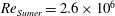 $Re_{\mathit{Sumer}}=2.6\times 10^{6}$
and
$Re_{\mathit{Sumer}}=2.6\times 10^{6}$
and
 $({\it\delta}=4.75\times 10^{-4},{\it\epsilon}=0.5)$
, corresponding to
$({\it\delta}=4.75\times 10^{-4},{\it\epsilon}=0.5)$
, corresponding to
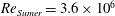 $Re_{\mathit{Sumer}}=3.6\times 10^{6}$
and did not observe any sign of instability in the acceleration region. Ozdemir et al. (Reference Ozdemir, Hsu and Balachandar2013) conjectured that for sufficiently strong perturbations a nonlinear instability can develop in front of the crest for Reynolds numbers larger than
$Re_{\mathit{Sumer}}=3.6\times 10^{6}$
and did not observe any sign of instability in the acceleration region. Ozdemir et al. (Reference Ozdemir, Hsu and Balachandar2013) conjectured that for sufficiently strong perturbations a nonlinear instability can develop in front of the crest for Reynolds numbers larger than
 $Re_{\mathit{Sumer}}=1.1\times 10^{6}$
, but did not observe any flow transition in front of the crest.
$Re_{\mathit{Sumer}}=1.1\times 10^{6}$
, but did not observe any flow transition in front of the crest.
We shall relate these findings to the present results. There are of course differences in the present work to the works by Vittori & Blondeaux (Reference Vittori and Blondeaux2008, Reference Vittori and Blondeaux2011), Ozdemir et al. (Reference Ozdemir, Hsu and Balachandar2013) and Sumer et al. (Reference Sumer, Jensen, Sørensen, Fredsøe, Liu and Carstensen2010). As stated in § 2.1 we start with a more accurate description of the outer flow than what was used in the previous studies. In addition, we do not neglect the nonlinear and non-parallel effects in the boundary layer. Moreover, the references considered temporal growth of instabilities, whereas the present study focuses on spatial growth. A more crucial difference is that Vittori & Blondeaux (Reference Vittori and Blondeaux2008, Reference Vittori and Blondeaux2011) in their simulations and Sumer et al. (Reference Sumer, Jensen, Sørensen, Fredsøe, Liu and Carstensen2010) in their experiments did not directly control the amplitude of the perturbation which might lead to a retarded appearance of the instability in their simulations and experiments, respectively. The importance of this point should not be underestimated and we shall discuss it in more detail below.
Concerning the appearance of instabilities in front of the crest, the question of whether there exists a nonlinear instability mechanism in front of the crest for this boundary layer as conjectured by Ozdemir et al. (Reference Ozdemir, Hsu and Balachandar2013) cannot be answered by the present method. Linear instability is, however, possible in front of the crest and we observe that the neutral curve for the case
 $({\it\delta}=10^{-4},{\it\epsilon}=0.4)$
in figure 8 is the first to cross the line
$({\it\delta}=10^{-4},{\it\epsilon}=0.4)$
in figure 8 is the first to cross the line
 ${\it\xi}=0$
. This case corresponds to a Reynolds number
${\it\xi}=0$
. This case corresponds to a Reynolds number
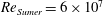 $Re_{\mathit{Sumer}}=6\times 10^{7}$
, which is an order of magnitude larger than what Sumer et al. (Reference Sumer, Jensen, Sørensen, Fredsøe, Liu and Carstensen2010) found and what Ozdemir et al. (Reference Ozdemir, Hsu and Balachandar2013) reported to be the lower bound in order to observe nonlinear growth in front of the crest. If the observed irregularities in front of the crest in Sumer et al. (Reference Sumer, Jensen, Sørensen, Fredsøe, Liu and Carstensen2010) have their origin in a nonlinear growth mechanism and whether this mechanism is strong enough or not (as Ozdemir et al.
Reference Ozdemir, Hsu and Balachandar2013 suggested) to induce a bypass transition is impossible to say without further knowledge of the experimental conditions. Concerning the quantitative discrepancy between the critical Reynolds numbers in the works by Vittori & Blondeaux (Reference Vittori and Blondeaux2008, Reference Vittori and Blondeaux2011), Ozdemir et al. (Reference Ozdemir, Hsu and Balachandar2013) and Sumer et al. (Reference Sumer, Jensen, Sørensen, Fredsøe, Liu and Carstensen2010), we discussed the cases
$Re_{\mathit{Sumer}}=6\times 10^{7}$
, which is an order of magnitude larger than what Sumer et al. (Reference Sumer, Jensen, Sørensen, Fredsøe, Liu and Carstensen2010) found and what Ozdemir et al. (Reference Ozdemir, Hsu and Balachandar2013) reported to be the lower bound in order to observe nonlinear growth in front of the crest. If the observed irregularities in front of the crest in Sumer et al. (Reference Sumer, Jensen, Sørensen, Fredsøe, Liu and Carstensen2010) have their origin in a nonlinear growth mechanism and whether this mechanism is strong enough or not (as Ozdemir et al.
Reference Ozdemir, Hsu and Balachandar2013 suggested) to induce a bypass transition is impossible to say without further knowledge of the experimental conditions. Concerning the quantitative discrepancy between the critical Reynolds numbers in the works by Vittori & Blondeaux (Reference Vittori and Blondeaux2008, Reference Vittori and Blondeaux2011), Ozdemir et al. (Reference Ozdemir, Hsu and Balachandar2013) and Sumer et al. (Reference Sumer, Jensen, Sørensen, Fredsøe, Liu and Carstensen2010), we discussed the cases
 ${\it\delta}=8\times 10^{-4}$
and
${\it\delta}=8\times 10^{-4}$
and
 ${\it\epsilon}=0.1,0.2,0.3,0.4$
above (cf. figures 7 and 11 and table 1). These cases have also been investigated by Vittori & Blondeaux (Reference Vittori and Blondeaux2008, Reference Vittori and Blondeaux2011). In figure 1 in Vittori & Blondeaux (Reference Vittori and Blondeaux2011), time profiles of the horizontal velocity component at a point in space are plotted. In addition, the case
${\it\epsilon}=0.1,0.2,0.3,0.4$
above (cf. figures 7 and 11 and table 1). These cases have also been investigated by Vittori & Blondeaux (Reference Vittori and Blondeaux2008, Reference Vittori and Blondeaux2011). In figure 1 in Vittori & Blondeaux (Reference Vittori and Blondeaux2011), time profiles of the horizontal velocity component at a point in space are plotted. In addition, the case
 ${\it\epsilon}=0.1$
has been considered stable by both Sumer et al. (Reference Sumer, Jensen, Sørensen, Fredsøe, Liu and Carstensen2010) and Vittori & Blondeaux (Reference Vittori and Blondeaux2011) (see figure 5 in Vittori & Blondeaux Reference Vittori and Blondeaux2011). The cases
${\it\epsilon}=0.1$
has been considered stable by both Sumer et al. (Reference Sumer, Jensen, Sørensen, Fredsøe, Liu and Carstensen2010) and Vittori & Blondeaux (Reference Vittori and Blondeaux2011) (see figure 5 in Vittori & Blondeaux Reference Vittori and Blondeaux2011). The cases
 ${\it\epsilon}=0.3$
and
${\it\epsilon}=0.3$
and
 ${\it\epsilon}=0.4$
, on the other hand, were found to be unstable by both references. However, the case
${\it\epsilon}=0.4$
, on the other hand, were found to be unstable by both references. However, the case
 ${\it\epsilon}=0.2$
was classified unstable by Sumer et al. (Reference Sumer, Jensen, Sørensen, Fredsøe, Liu and Carstensen2010), whereas Vittori & Blondeaux (Reference Vittori and Blondeaux2011) deemed it stable. Ozdemir et al. (Reference Ozdemir, Hsu and Balachandar2013), on the other hand, would consider this case as disturbed laminar with the possible appearance of roller pairs.
${\it\epsilon}=0.2$
was classified unstable by Sumer et al. (Reference Sumer, Jensen, Sørensen, Fredsøe, Liu and Carstensen2010), whereas Vittori & Blondeaux (Reference Vittori and Blondeaux2011) deemed it stable. Ozdemir et al. (Reference Ozdemir, Hsu and Balachandar2013), on the other hand, would consider this case as disturbed laminar with the possible appearance of roller pairs.
In figure 11 the growth of the critical Tollmien–Schlichting wave is shown. The amplifications of the Tollmien–Schlichting waves at
 ${\it\xi}=19.5$
, as compared with the minimum value at
${\it\xi}=19.5$
, as compared with the minimum value at
 ${\it\xi}_{c}$
, are listed in table 1. If we assume that the Tollmien–Schlichting waves start to roll up into vortices (triggering of the secondary instability) once their amplitude has grown to a value of 1 % of the mean flow (which we set to unity for simplicity), the amplification (
${\it\xi}_{c}$
, are listed in table 1. If we assume that the Tollmien–Schlichting waves start to roll up into vortices (triggering of the secondary instability) once their amplitude has grown to a value of 1 % of the mean flow (which we set to unity for simplicity), the amplification (
 $10^{5}$
) for the unstable case
$10^{5}$
) for the unstable case
 ${\it\epsilon}=0.2$
in table 1, tells us that the background noise in the experiments in Sumer et al. (Reference Sumer, Jensen, Sørensen, Fredsøe, Liu and Carstensen2010) was higher than
${\it\epsilon}=0.2$
in table 1, tells us that the background noise in the experiments in Sumer et al. (Reference Sumer, Jensen, Sørensen, Fredsøe, Liu and Carstensen2010) was higher than
 $10^{-7}$
. On the other hand, the case
$10^{-7}$
. On the other hand, the case
 ${\it\epsilon}=0.1$
(amplification:
${\it\epsilon}=0.1$
(amplification:
 $10^{2.7}$
) was classified stable. Therefore, the background noise level in the experiments by Sumer et al. (Reference Sumer, Jensen, Sørensen, Fredsøe, Liu and Carstensen2010) might have been between
$10^{2.7}$
) was classified stable. Therefore, the background noise level in the experiments by Sumer et al. (Reference Sumer, Jensen, Sørensen, Fredsøe, Liu and Carstensen2010) might have been between
 $10^{-7}$
and
$10^{-7}$
and
 $10^{-4.7}$
. A similar reasoning finds the background noise in the simulations by Vittori & Blondeaux (Reference Vittori and Blondeaux2008, Reference Vittori and Blondeaux2011) to be between
$10^{-4.7}$
. A similar reasoning finds the background noise in the simulations by Vittori & Blondeaux (Reference Vittori and Blondeaux2008, Reference Vittori and Blondeaux2011) to be between
 $10^{-8.5}$
and
$10^{-8.5}$
and
 $10^{-7}$
. Since linear stability predicts a strong decay of the perturbations in the acceleration region, the initial
$10^{-7}$
. Since linear stability predicts a strong decay of the perturbations in the acceleration region, the initial
 $10^{-4}$
amplitude perturbation, which Vittori & Blondeaux (Reference Vittori and Blondeaux2008, Reference Vittori and Blondeaux2011) imposed onto the initial condition before the solitary wave arrived, should have decayed by the time the critical position was reached to values much lower than the
$10^{-4}$
amplitude perturbation, which Vittori & Blondeaux (Reference Vittori and Blondeaux2008, Reference Vittori and Blondeaux2011) imposed onto the initial condition before the solitary wave arrived, should have decayed by the time the critical position was reached to values much lower than the
 $10^{-7}$
estimated above. The NS solver used by Vittori & Blondeaux (Reference Vittori and Blondeaux2008, Reference Vittori and Blondeaux2011) and Blondeaux et al. (Reference Blondeaux, Pralits and Vittori2012) may have produced a certain level of numerical noise, which might have provided a sufficient level at
$10^{-7}$
estimated above. The NS solver used by Vittori & Blondeaux (Reference Vittori and Blondeaux2008, Reference Vittori and Blondeaux2011) and Blondeaux et al. (Reference Blondeaux, Pralits and Vittori2012) may have produced a certain level of numerical noise, which might have provided a sufficient level at
 ${\it\xi}_{c}$
for instabilities to become visible. We find support for this presumption in figure 4 in Blondeaux et al. (Reference Blondeaux, Pralits and Vittori2012), where the level of kinetic energy of the perturbation seems to stay on a stable level of around
${\it\xi}_{c}$
for instabilities to become visible. We find support for this presumption in figure 4 in Blondeaux et al. (Reference Blondeaux, Pralits and Vittori2012), where the level of kinetic energy of the perturbation seems to stay on a stable level of around
 $10^{-8}{-}10^{-9}$
for all cases of
$10^{-8}{-}10^{-9}$
for all cases of
 ${\it\epsilon}$
, before arriving at the critical position. Several reasons for the numerical source of noise are possible, such as truncation errors or incomplete pressure solutions. Overall, the triggering mechanism of the instability in these references is not well controlled. A better approach has been chosen by Ozdemir et al. (Reference Ozdemir, Hsu and Balachandar2013) where five different intensities of white noise have been introduced at the beginning of a direct numerical simulation. In addition they followed the evolution of the root-mean-square velocity during the course of the simulations. Although being a major improvement over the approach by Vittori & Blondeaux (Reference Vittori and Blondeaux2008, Reference Vittori and Blondeaux2011), the results cannot be transferred to the case where a constant level of background noise is present, as for example in laboratories. As predicted by the present linear stability the perturbations in Ozdemir et al. (Reference Ozdemir, Hsu and Balachandar2013) underwent strong decay before growing again. As a consequence of their analysis, Ozdemir et al. (Reference Ozdemir, Hsu and Balachandar2013) also obtained a new set of critical Reynolds numbers
${\it\epsilon}$
, before arriving at the critical position. Several reasons for the numerical source of noise are possible, such as truncation errors or incomplete pressure solutions. Overall, the triggering mechanism of the instability in these references is not well controlled. A better approach has been chosen by Ozdemir et al. (Reference Ozdemir, Hsu and Balachandar2013) where five different intensities of white noise have been introduced at the beginning of a direct numerical simulation. In addition they followed the evolution of the root-mean-square velocity during the course of the simulations. Although being a major improvement over the approach by Vittori & Blondeaux (Reference Vittori and Blondeaux2008, Reference Vittori and Blondeaux2011), the results cannot be transferred to the case where a constant level of background noise is present, as for example in laboratories. As predicted by the present linear stability the perturbations in Ozdemir et al. (Reference Ozdemir, Hsu and Balachandar2013) underwent strong decay before growing again. As a consequence of their analysis, Ozdemir et al. (Reference Ozdemir, Hsu and Balachandar2013) also obtained a new set of critical Reynolds numbers
 $Re_{\mathit{Sumer}}$
.
$Re_{\mathit{Sumer}}$
.
The present investigation is different, it solves the governing equations, i.e. the Orr–Sommerfeld and the PSE, for the perturbations, the Tollmien–Schlichting waves themselves. The amplification of the Tollmien–Schlichting waves can therefore be computed independently from any given initial level of noise, as long as the initial level is small. Since the initial amplitude is crucial for the visual appearance of the perturbation or observation of transition (triggering of the secondary instability), a result from the present analysis is that classifications such as that presented in figure 5 of Sumer et al. (Reference Sumer, Jensen, Sørensen, Fredsøe, Liu and Carstensen2010), figure 5 of Vittori & Blondeaux (Reference Vittori and Blondeaux2011) or in § 4.4 of Ozdemir et al. (Reference Ozdemir, Hsu and Balachandar2013), or the determination of critical parameters
 $({\it\delta}_{c},{\it\epsilon}_{c})$
in Blondeaux et al. (Reference Blondeaux, Pralits and Vittori2012), need to be taken with care. The flow is convectively unstable and acts as a broadband amplifier, similar to the Blasius boundary layer (Herbert Reference Herbert1988).
$({\it\delta}_{c},{\it\epsilon}_{c})$
in Blondeaux et al. (Reference Blondeaux, Pralits and Vittori2012), need to be taken with care. The flow is convectively unstable and acts as a broadband amplifier, similar to the Blasius boundary layer (Herbert Reference Herbert1988).
As mentioned above, in figure 13 isolines for the amplification of the critical Tollmien–Schlichting waves are plotted. Knowing the initial amplitude at the neutral curve of the critical Tollmien–Schlichting wave for an experiment or a direct numerical simulation, we might by means of the isolines predict whether disturbances become visible or not. In addition to the isolines, we plotted lines given for the critical Reynolds numbers
 $Re_{\mathit{Sumer}}=2\times 10^{6}$
and
$Re_{\mathit{Sumer}}=2\times 10^{6}$
and
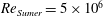 $Re_{\mathit{Sumer}}=5\times 10^{6}$
. For small values of
$Re_{\mathit{Sumer}}=5\times 10^{6}$
. For small values of
 ${\it\delta}$
and
${\it\delta}$
and
 ${\it\epsilon}$
, we observe that the lines seem to coincide with the isolines for an amplification of
${\it\epsilon}$
, we observe that the lines seem to coincide with the isolines for an amplification of
 $10^{4}$
and
$10^{4}$
and
 $10^{7}$
, respectively. However, as
$10^{7}$
, respectively. However, as
 ${\it\epsilon}$
and
${\it\epsilon}$
and
 ${\it\delta}$
increase the lines do not follow these isolines anymore. As mentioned in § 2.1, the deviation for increasing
${\it\delta}$
increase the lines do not follow these isolines anymore. As mentioned in § 2.1, the deviation for increasing
 ${\it\epsilon}$
reflects the limited accuracy of the first-order approximation of the outer flow. The deviation for increasing
${\it\epsilon}$
reflects the limited accuracy of the first-order approximation of the outer flow. The deviation for increasing
 ${\it\delta}$
, on the other hand, is due to non-parallel effects becoming significant. For small values of
${\it\delta}$
, on the other hand, is due to non-parallel effects becoming significant. For small values of
 ${\it\delta}$
and
${\it\delta}$
and
 ${\it\epsilon}$
, the amplification of Tollmien–Schlichting waves gives a theoretical explanation for the appearance of transition beyond a critical
${\it\epsilon}$
, the amplification of Tollmien–Schlichting waves gives a theoretical explanation for the appearance of transition beyond a critical
 $Re_{\mathit{Sumer}}$
in the experiments by Sumer et al. (Reference Sumer, Jensen, Sørensen, Fredsøe, Liu and Carstensen2010) or the simulations by Vittori & Blondeaux (Reference Vittori and Blondeaux2008, Reference Vittori and Blondeaux2011) and Ozdemir et al. (Reference Ozdemir, Hsu and Balachandar2013). The stability properties of the flow are, however, more complex, since neutral curves, critical positions, critical wavelengths, critical frequencies, etc., can be different for a given
$Re_{\mathit{Sumer}}$
in the experiments by Sumer et al. (Reference Sumer, Jensen, Sørensen, Fredsøe, Liu and Carstensen2010) or the simulations by Vittori & Blondeaux (Reference Vittori and Blondeaux2008, Reference Vittori and Blondeaux2011) and Ozdemir et al. (Reference Ozdemir, Hsu and Balachandar2013). The stability properties of the flow are, however, more complex, since neutral curves, critical positions, critical wavelengths, critical frequencies, etc., can be different for a given
 $Re_{\mathit{Sumer}}$
.
$Re_{\mathit{Sumer}}$
.
Most important, however, is the fact that the flow may appear to be stable (in the sense that transition does not occur) for a specific
 $Re_{\mathit{Sumer}}$
or
$Re_{\mathit{Sumer}}$
or
 $({\it\delta}_{c},{\it\epsilon}_{c})$
during one experimental run, whereas it appears to be unstable during another run. This observation has been made by Pedersen et al. (Reference Pedersen, Lindstrøm, Bertelsen, Jensen, Laskovski and Sælevik2013) for a related problem, namely the boundary layer of a solitary wave running up a sloping beach, where the occurrence of irregularities was not strictly repeatable. In fact, unless the disturbance level is actively controlled we do not believe that experimental repeatability for a flow transition of this type can be obtained.
$({\it\delta}_{c},{\it\epsilon}_{c})$
during one experimental run, whereas it appears to be unstable during another run. This observation has been made by Pedersen et al. (Reference Pedersen, Lindstrøm, Bertelsen, Jensen, Laskovski and Sælevik2013) for a related problem, namely the boundary layer of a solitary wave running up a sloping beach, where the occurrence of irregularities was not strictly repeatable. In fact, unless the disturbance level is actively controlled we do not believe that experimental repeatability for a flow transition of this type can be obtained.
3.1.3. Direct numerical simulation
In the analysis above (cf. § 3.1), results have been generated by model equations; namely the OSE and the PSE. In the present subsection a direct numerical simulation based on first principles is performed for validation. Our approach is very different from that of Vittori & Blondeaux (Reference Vittori and Blondeaux2008, Reference Vittori and Blondeaux2011) or Ozdemir et al. (Reference Ozdemir, Hsu and Balachandar2013), in the sense that the perturbation is carefully controlled and that we, in contrast to Vittori & Blondeaux (Reference Vittori and Blondeaux2008, Reference Vittori and Blondeaux2011), employ a high-accuracy solution method for the NS equations. We note that different types of NS solvers might give different sets of allegedly critical parameters
 $({\it\epsilon}_{c},{\it\delta}_{c})$
depending on their truncation errors, numerical dissipation rates etc.
$({\it\epsilon}_{c},{\it\delta}_{c})$
depending on their truncation errors, numerical dissipation rates etc.
As mentioned in § 2, the present direct numerical simulations are performed using a method developed by Fasel (Reference Fasel1976, Reference Fasel2002) to investigate the stability of the Blasius boundary layer. Thereby a Tollmien–Schlichting wave is introduced at the inlet of the simulation domain and its evolution is monitored.

Figure 16. (a) Stability domain for the case
 ${\it\epsilon}=0.4$
and
${\it\epsilon}=0.4$
and
 ${\it\delta}=8\times 10^{-4}$
. (b) Horizontal perturbation
${\it\delta}=8\times 10^{-4}$
. (b) Horizontal perturbation
 $u^{\prime }$
of the horizontal velocity component recorded at a distance
$u^{\prime }$
of the horizontal velocity component recorded at a distance
 $y=0.4943$
from the wall for a Tollmien–Schlichting wave of
$y=0.4943$
from the wall for a Tollmien–Schlichting wave of
 ${\it\omega}=0.24$
computed by means of the NS solver. (c) Amplification of the Tollmien–Schlichting wave with
${\it\omega}=0.24$
computed by means of the NS solver. (c) Amplification of the Tollmien–Schlichting wave with
 ${\it\omega}=0.24$
computed by means of the OSE solver, the PSE solver and the NS solver.
${\it\omega}=0.24$
computed by means of the OSE solver, the PSE solver and the NS solver.
Figure 16 shows three plots for the case
 ${\it\epsilon}=0.4$
and
${\it\epsilon}=0.4$
and
 ${\it\delta}=8\times 10^{-4}$
. In figure 16(a), the stability domain of the flow, computed using the PSE solver, has been plotted by the criterion of maximum or minimum amplitude
${\it\delta}=8\times 10^{-4}$
. In figure 16(a), the stability domain of the flow, computed using the PSE solver, has been plotted by the criterion of maximum or minimum amplitude
 $A$
in (2.27). We now pick a particular frequency
$A$
in (2.27). We now pick a particular frequency
 ${\it\omega}$
and follow the evolution of a Tollmien–Schlichting wave with this frequency. In figure 16(b), we have chosen the Tollmien–Schlichting wave with the critical frequency
${\it\omega}$
and follow the evolution of a Tollmien–Schlichting wave with this frequency. In figure 16(b), we have chosen the Tollmien–Schlichting wave with the critical frequency
 ${\it\omega}_{c}=0.24$
. The velocity field
${\it\omega}_{c}=0.24$
. The velocity field
 $u({\it\xi},y,t)$
at a specific point in time
$u({\it\xi},y,t)$
at a specific point in time
 $t$
computed by the NS solver, allows us to compute the perturbation velocity
$t$
computed by the NS solver, allows us to compute the perturbation velocity
 $u^{\prime }({\it\xi},y,t)$
by subtracting the base flow
$u^{\prime }({\it\xi},y,t)$
by subtracting the base flow
 $U_{\mathit{base}}({\it\xi},y)$
from the velocity field:
$U_{\mathit{base}}({\it\xi},y)$
from the velocity field:
 $$\begin{eqnarray}u^{\prime }=u-U_{\mathit{base}}.\end{eqnarray}$$
In figure 16(b), a transect of
 $u^{\prime }$
at
$u^{\prime }$
at
 $y=0.4943$
is plotted. We clearly observe a sinusoidal wave which decays until it reaches the critical position
$y=0.4943$
is plotted. We clearly observe a sinusoidal wave which decays until it reaches the critical position
 ${\it\xi}_{c}=0.82$
and then starts to grow, albeit slowly at the beginning. This qualitative picture can be analysed further. Using the solution
${\it\xi}_{c}=0.82$
and then starts to grow, albeit slowly at the beginning. This qualitative picture can be analysed further. Using the solution
 $u(x,y,t)$
by the NS solver, we compute the amplitude of the Tollmien–Schlichting wave by means of the envelope of
$u(x,y,t)$
by the NS solver, we compute the amplitude of the Tollmien–Schlichting wave by means of the envelope of
 $u^{\prime }$
at its maximum, i.e.
$u^{\prime }$
at its maximum, i.e.
 $$\begin{eqnarray}A({\it\xi})=\max _{t,y}|u^{\prime }({\it\xi},y,t)|.\end{eqnarray}$$
This envelope can then be compared with the resulting amplifications using the PSE and the OSE, computed by means of (2.27) and (2.19), respectively. The result of this comparison is depicted in figure 16(c). All three methods predict first a decay of the Tollmien–Schlichting wave followed by growth. The results by the NS solver and by the PSE solver agree remarkably well. The results by the Orr–Sommerfeld solver on the other hand display an earlier growth of the Tollmien–Schlichting wave compared to the other two solvers, a feature which was also observed by looking at the stability domains in the subsection above. This indicates that non-parallel effects do lead to quantitative differences.
A closer look at figure 16(c) reveals that for
 ${\it\xi}\gtrsim 2.5$
the amplification curves computed by the parabolized stability method and the NS solver start to mildly deviate. This indicates that the effect of nonlinearity becomes increasingly significant. We can study this effect further. By introducing a superposition of Tollmien–Schlichting waves at the inlet of our computational domain, we can monitor the perturbation velocity
${\it\xi}\gtrsim 2.5$
the amplification curves computed by the parabolized stability method and the NS solver start to mildly deviate. This indicates that the effect of nonlinearity becomes increasingly significant. We can study this effect further. By introducing a superposition of Tollmien–Schlichting waves at the inlet of our computational domain, we can monitor the perturbation velocity
 $u^{\prime }$
in horizontal direction at different locations further downstream. The perturbation velocity
$u^{\prime }$
in horizontal direction at different locations further downstream. The perturbation velocity
 $u^{\prime }$
of the Tollmien–Schlichting waves introduced at the inlet is thus given by
$u^{\prime }$
of the Tollmien–Schlichting waves introduced at the inlet is thus given by
 $$\begin{eqnarray}u^{\prime }({\it\xi}_{inlet},y,t)=\mathop{\sum }_{k=1}^{N_{{\it\omega}}}\text{Re}\{A_{k}u_{k}(y)\exp \text{i}\left({\it\alpha}_{k}{\it\xi}_{inlet}-{\it\omega}_{k}t\right)\}\end{eqnarray}$$
where
 $N_{{\it\omega}}$
is the number of Tollmien–Schlichting waves used,
$N_{{\it\omega}}$
is the number of Tollmien–Schlichting waves used,
 $u_{k}$
is the shape function at the inlet, computed by the PSE solver, and
$u_{k}$
is the shape function at the inlet, computed by the PSE solver, and
 ${\it\alpha}_{k}=\text{Im}(a_{k})$
is the wavenumber corresponding to the frequency
${\it\alpha}_{k}=\text{Im}(a_{k})$
is the wavenumber corresponding to the frequency
 ${\it\omega}_{k}$
. The frequencies
${\it\omega}_{k}$
. The frequencies
 ${\it\omega}_{k}$
have been chosen such that
${\it\omega}_{k}$
have been chosen such that
 ${\it\omega}_{1}$
equals
${\it\omega}_{1}$
equals
 $0.15$
and
$0.15$
and
 ${\it\omega}_{N_{{\it\omega}}}$
equals
${\it\omega}_{N_{{\it\omega}}}$
equals
 $0.35$
with
$0.35$
with
 $N_{{\it\omega}}=61$
. They are distributed such that we have an equidistant spacing of Fourier modes:
$N_{{\it\omega}}=61$
. They are distributed such that we have an equidistant spacing of Fourier modes:
 $$\begin{eqnarray}{\it\omega}_{k}={\rm\Delta}{\it\omega}(k-1)+{\it\omega}_{1},\end{eqnarray}$$
where
 ${\rm\Delta}{\it\omega}=({\it\omega}_{N_{{\it\omega}}}-{\it\omega}_{1})/(N_{{\it\omega}}-1)$
. The initial amplitude
${\rm\Delta}{\it\omega}=({\it\omega}_{N_{{\it\omega}}}-{\it\omega}_{1})/(N_{{\it\omega}}-1)$
. The initial amplitude
 $A_{k}$
of each Fourier mode is set uniformly to
$A_{k}$
of each Fourier mode is set uniformly to
 $A_{k}=5\times 10^{-4}/N_{{\it\omega}}$
. The positions at which we monitor the perturbation velocity
$A_{k}=5\times 10^{-4}/N_{{\it\omega}}$
. The positions at which we monitor the perturbation velocity
 $u^{\prime }$
are given by
$u^{\prime }$
are given by
 ${\it\xi}=2.40,2.96$
and
${\it\xi}=2.40,2.96$
and
 $3.12$
. At these locations we record the time series of
$3.12$
. At these locations we record the time series of
 $u^{\prime }$
at a distance of
$u^{\prime }$
at a distance of
 $1.64$
from the wall. A decomposition of the signal into its Fourier modes allows us to find the amplitudes
$1.64$
from the wall. A decomposition of the signal into its Fourier modes allows us to find the amplitudes
 $A_{k}$
at these downstream locations. Figure 17 presents the amplitudes
$A_{k}$
at these downstream locations. Figure 17 presents the amplitudes
 $A_{k}$
as a function of
$A_{k}$
as a function of
 ${\it\omega}_{k}$
. In addition, we plot the amplitudes
${\it\omega}_{k}$
. In addition, we plot the amplitudes
 $A_{k}$
predicted by the present linear PSE solver for comparison. We observe that the signal received further downstream, consists of discrete spikes separated by
$A_{k}$
predicted by the present linear PSE solver for comparison. We observe that the signal received further downstream, consists of discrete spikes separated by
 ${\rm\Delta}{\it\omega}$
, indicating that the perturbation
${\rm\Delta}{\it\omega}$
, indicating that the perturbation
 $u^{\prime }$
at these locations has its origin in the perturbation introduced at the inlet. When repeating the computation at lower spatial and temporal resolutions, the simulation displays the emergence of a continuous spectrum with modes filling the space between the spikes for the locations further downstream. These modes which are absent for finer resolutions have probably their origin in the truncation error of the simulation growing in parallel to the Tollmien–Schlichting waves. Returning to figure 17, for the direct numerical simulation and the PSE we observe a strong growth of the individual modes for increasing
$u^{\prime }$
at these locations has its origin in the perturbation introduced at the inlet. When repeating the computation at lower spatial and temporal resolutions, the simulation displays the emergence of a continuous spectrum with modes filling the space between the spikes for the locations further downstream. These modes which are absent for finer resolutions have probably their origin in the truncation error of the simulation growing in parallel to the Tollmien–Schlichting waves. Returning to figure 17, for the direct numerical simulation and the PSE we observe a strong growth of the individual modes for increasing
 ${\it\xi}$
. Growth is strongest for modes around
${\it\xi}$
. Growth is strongest for modes around
 ${\it\omega}=0.26$
which is somewhat higher than the critical frequency (
${\it\omega}=0.26$
which is somewhat higher than the critical frequency (
 ${\it\omega}_{c}=0.24$
). We remark that we measure the amplitude here not by criterion (2.27) but at a specific location in
${\it\omega}_{c}=0.24$
). We remark that we measure the amplitude here not by criterion (2.27) but at a specific location in
 $y$
. For
$y$
. For
 ${\it\xi}=2.40$
, we see that the amplitudes computed by the NS solver and the linear parabolized equation solver are agreeing well. However, further downwards,
${\it\xi}=2.40$
, we see that the amplitudes computed by the NS solver and the linear parabolized equation solver are agreeing well. However, further downwards,
 ${\it\xi}=2.96$
, we observe that the amplitudes computed by the NS solver tend to be somewhat lower than predicted by the PSE solver. This discrepancy is even more emphasized for
${\it\xi}=2.96$
, we observe that the amplitudes computed by the NS solver tend to be somewhat lower than predicted by the PSE solver. This discrepancy is even more emphasized for
 ${\it\xi}=3.12$
, where the modes computed by direct numerical simulation are significantly lower than the modes computed by the PSE solver. The spectrum reflects the discontinuity of the initial distribution, displaying a sudden jump at
${\it\xi}=3.12$
, where the modes computed by direct numerical simulation are significantly lower than the modes computed by the PSE solver. The spectrum reflects the discontinuity of the initial distribution, displaying a sudden jump at
 ${\it\omega}=0.15$
and
${\it\omega}=0.15$
and
 ${\it\omega}=3.5$
. However, we observe for
${\it\omega}=3.5$
. However, we observe for
 ${\it\xi}=2.96$
and
${\it\xi}=2.96$
and
 ${\it\xi}=3.12$
, the appearance of (significant) modes outside of the interval
${\it\xi}=3.12$
, the appearance of (significant) modes outside of the interval
 $[{\it\omega}_{1},{\it\omega}_{N_{{\it\omega}}}]$
, but still with a spacing given by
$[{\it\omega}_{1},{\it\omega}_{N_{{\it\omega}}}]$
, but still with a spacing given by
 ${\rm\Delta}{\it\omega}$
. In particular for
${\rm\Delta}{\it\omega}$
. In particular for
 ${\it\xi}=3.12$
, we observe two additional peaks at
${\it\xi}=3.12$
, we observe two additional peaks at
 ${\it\omega}=0$
and
${\it\omega}=0$
and
 ${\it\omega}=5.3$
, located respectively at zero or two times the frequency of the maximum amplitude. As can be seen from the neutral curve in figure 16(a), this is in contrast to the linear analysis which does not predict any growth for frequencies around
${\it\omega}=5.3$
, located respectively at zero or two times the frequency of the maximum amplitude. As can be seen from the neutral curve in figure 16(a), this is in contrast to the linear analysis which does not predict any growth for frequencies around
 ${\it\omega}=0$
. As such the primary effect of nonlinearity is to distribute energy away from modes of maximum amplification.
${\it\omega}=0$
. As such the primary effect of nonlinearity is to distribute energy away from modes of maximum amplification.
We remark that the present nonlinear study is limited as we only present results for a particular spectrum, namely a uniform initial distribution of Tollmien–Schlichting waves with frequency spacing
 ${\rm\Delta}{\it\omega}$
. It needs to be noted that for the simulations, each of these modes undergoes a phase of decay first, before reaching the neutral curve. The amount by which each mode has decayed by the time it reaches the neutral curve is varying. This is different to the experimental situation where it is assumed that a certain level of noise is present everywhere in the set up, the frequency distribution of this noise being unknown. We emphasize that the present PSE solver is linear. A nonlinear version, as derived by Bertolotti et al. (Reference Bertolotti, Herbert and Spalart1992), would be able to account for the interaction between Tollmien–Schlichting modes. In addition, we only consider two dimensional disturbances, leaving aside any possible interaction with spanwise modes. Nevertheless, despite its limitation, this nonlinear study reveals that the present linear stability analysis describes accurately the early growth of the perturbations destabilizing the flow.
${\rm\Delta}{\it\omega}$
. It needs to be noted that for the simulations, each of these modes undergoes a phase of decay first, before reaching the neutral curve. The amount by which each mode has decayed by the time it reaches the neutral curve is varying. This is different to the experimental situation where it is assumed that a certain level of noise is present everywhere in the set up, the frequency distribution of this noise being unknown. We emphasize that the present PSE solver is linear. A nonlinear version, as derived by Bertolotti et al. (Reference Bertolotti, Herbert and Spalart1992), would be able to account for the interaction between Tollmien–Schlichting modes. In addition, we only consider two dimensional disturbances, leaving aside any possible interaction with spanwise modes. Nevertheless, despite its limitation, this nonlinear study reveals that the present linear stability analysis describes accurately the early growth of the perturbations destabilizing the flow.

Figure 17. Fourier modes of the perturbation velocity
 $u^{\prime }$
computed by direct numerical simulation (NS) and linear PSE at
$u^{\prime }$
computed by direct numerical simulation (NS) and linear PSE at
 $y=1.64$
and different values of
$y=1.64$
and different values of
 ${\it\xi}$
for the case
${\it\xi}$
for the case
 ${\it\epsilon}=0.4$
and
${\it\epsilon}=0.4$
and
 ${\it\delta}=8\times 10^{-4}$
.
${\it\delta}=8\times 10^{-4}$
.
3.2. Linear stability analysis for internal solitary waves
3.2.1. Stability regions and amplifications
The boundary layer under surface solitary waves is characterized by two parameters, the amplitude
 ${\it\epsilon}$
and the parameter
${\it\epsilon}$
and the parameter
 ${\it\delta}$
. For internal solitary waves, as sketched in figure 2, the system contains two more parameters accounting for the density ratio and the depth ratio between the two layers. In the following we use the lower layer density
${\it\delta}$
. For internal solitary waves, as sketched in figure 2, the system contains two more parameters accounting for the density ratio and the depth ratio between the two layers. In the following we use the lower layer density
 ${\it\rho}_{1}$
and the lower layer depth
${\it\rho}_{1}$
and the lower layer depth
 $h_{1}$
as parameters. The scaling is such that the upper layer density
$h_{1}$
as parameters. The scaling is such that the upper layer density
 ${\it\rho}_{2}$
is unity, whereas the upper layer depth is given by
${\it\rho}_{2}$
is unity, whereas the upper layer depth is given by
 $h_{2}=1-h_{1}$
. In addition, we consider waves of elevation (
$h_{2}=1-h_{1}$
. In addition, we consider waves of elevation (
 ${\it\epsilon}>0$
,
${\it\epsilon}>0$
,
 $h_{1}<h_{c}$
) and waves of depression (
$h_{1}<h_{c}$
) and waves of depression (
 ${\it\epsilon}<0$
,
${\it\epsilon}<0$
,
 $h_{1}>h_{c}$
), where
$h_{1}>h_{c}$
), where
 $h_{c}$
is the height of the critical level (Funakoshi & Oikawa Reference Funakoshi and Oikawa1986):
$h_{c}$
is the height of the critical level (Funakoshi & Oikawa Reference Funakoshi and Oikawa1986):
 $$\begin{eqnarray}h_{c}=\frac{\sqrt{{\it\rho}_{2}/{\it\rho}_{1}}}{1+\sqrt{{\it\rho}_{2}/{\it\rho}_{1}}}h_{0}.\end{eqnarray}$$
We compute the base flow
 $(U_{\mathit{base}},V_{\mathit{base}})$
using the present boundary-layer solver in combination with the method by Funakoshi & Oikawa (Reference Funakoshi and Oikawa1986). This flow is then the subject of the present linear stability analysis by means of the PSE. Profiles of the horizontal velocity component for a wave of elevation are displayed in figure 18. Qualitatively, the profiles are similar to those of a surface solitary wave. An inversion of the flow is observed in the deceleration region
$(U_{\mathit{base}},V_{\mathit{base}})$
using the present boundary-layer solver in combination with the method by Funakoshi & Oikawa (Reference Funakoshi and Oikawa1986). This flow is then the subject of the present linear stability analysis by means of the PSE. Profiles of the horizontal velocity component for a wave of elevation are displayed in figure 18. Qualitatively, the profiles are similar to those of a surface solitary wave. An inversion of the flow is observed in the deceleration region
 ${\it\xi}>0$
of the wave. Although we consider only two-layered fluids, fluids with a pycnocline with non-zero thickness can relatively well be approximated by a two-layered system, as long as the thickness of the pycnocline is small (cf. Carr et al.
Reference Carr, Davies and Shivaram2008). This can also be seen in figure 19, where we plotted the same time histories for the horizontal velocity as in Thiem et al. (Reference Thiem, Carr, Berntsen and Davies2011) for a wave of depression. The pycnocline of the present two-layered system lies in the centre of the middle layer of experiment ‘20538’ in Carr & Davies (Reference Carr and Davies2006). The scaling corresponds to that of Thiem et al. (Reference Thiem, Carr, Berntsen and Davies2011). The data has been taken by a digitization tool from figure 4(a) of Thiem et al. (Reference Thiem, Carr, Berntsen and Davies2011). Although the agreement between experimental data and numerical result is not excellent it is still reasonable in view of the uncertainties involved in such measurements. The amplitude is predicted somewhat lower than for the data. However, the agreement is still closer to the experimental data than for the numerical method of Thiem et al. (Reference Thiem, Carr, Berntsen and Davies2011).
${\it\xi}>0$
of the wave. Although we consider only two-layered fluids, fluids with a pycnocline with non-zero thickness can relatively well be approximated by a two-layered system, as long as the thickness of the pycnocline is small (cf. Carr et al.
Reference Carr, Davies and Shivaram2008). This can also be seen in figure 19, where we plotted the same time histories for the horizontal velocity as in Thiem et al. (Reference Thiem, Carr, Berntsen and Davies2011) for a wave of depression. The pycnocline of the present two-layered system lies in the centre of the middle layer of experiment ‘20538’ in Carr & Davies (Reference Carr and Davies2006). The scaling corresponds to that of Thiem et al. (Reference Thiem, Carr, Berntsen and Davies2011). The data has been taken by a digitization tool from figure 4(a) of Thiem et al. (Reference Thiem, Carr, Berntsen and Davies2011). Although the agreement between experimental data and numerical result is not excellent it is still reasonable in view of the uncertainties involved in such measurements. The amplitude is predicted somewhat lower than for the data. However, the agreement is still closer to the experimental data than for the numerical method of Thiem et al. (Reference Thiem, Carr, Berntsen and Davies2011).

Figure 18. Horizontal velocity profiles for the boundary-layer flow under an internal solitary wave of elevation with
 ${\it\epsilon}=0.1$
,
${\it\epsilon}=0.1$
,
 ${\it\delta}=0.0023$
,
${\it\delta}=0.0023$
,
 ${\it\rho}_{1}=1.25$
and
${\it\rho}_{1}=1.25$
and
 $h_{1}={\textstyle \frac{1}{3}}$
.
$h_{1}={\textstyle \frac{1}{3}}$
.

Figure 19. Time histories for the horizontal velocity in the boundary layer of a two-layered fluid corresponding to the case ‘20538’ of Carr & Davies (Reference Carr and Davies2006) at
 $z/h_{2}=0.1,0.2,0.4$
(wave of depression). The experimental data by Carr & Davies (Reference Carr and Davies2006) was scanned from Thiem et al. (Reference Thiem, Carr, Berntsen and Davies2011).
$z/h_{2}=0.1,0.2,0.4$
(wave of depression). The experimental data by Carr & Davies (Reference Carr and Davies2006) was scanned from Thiem et al. (Reference Thiem, Carr, Berntsen and Davies2011).

Figure 20. Stability domains for the wave of elevation case
 ${\it\epsilon}=0.1$
,
${\it\epsilon}=0.1$
,
 ${\it\delta}=10^{-3}$
and
${\it\delta}=10^{-3}$
and
 $h_{1}={\textstyle \frac{1}{3}}$
for different values of
$h_{1}={\textstyle \frac{1}{3}}$
for different values of
 ${\it\rho}_{1}$
.
${\it\rho}_{1}$
.

Figure 21. Amplification curves for the critical Tollmien–Schlichting waves for the cases in figure 20.
Carr & Davies (Reference Carr and Davies2010) concluded on the basis of their experiments that the boundary-layer flows of internal solitary waves are qualitatively similar to those of surface solitary waves. A quantitative comparison is, on the other hand, not straightforward, because of the additional parameters
 ${\it\rho}_{1}$
and
${\it\rho}_{1}$
and
 $h_{1}$
. However, the leading-order solution for the internal solitary wave in a two-layered fluid (Keulegan Reference Keulegan1953) is in the present scaling independent of the density ratio (we are very grateful to one anonymous referee for pointing this out). This can also be observed when we keep all parameters fixed and vary only
$h_{1}$
. However, the leading-order solution for the internal solitary wave in a two-layered fluid (Keulegan Reference Keulegan1953) is in the present scaling independent of the density ratio (we are very grateful to one anonymous referee for pointing this out). This can also be observed when we keep all parameters fixed and vary only
 ${\it\rho}_{1}$
. In figure 20, we plotted the neutral curves for the wave of elevation case
${\it\rho}_{1}$
. In figure 20, we plotted the neutral curves for the wave of elevation case
 ${\it\epsilon}=0.1$
,
${\it\epsilon}=0.1$
,
 ${\it\delta}=10^{-3}$
and
${\it\delta}=10^{-3}$
and
 $h_{1}={\textstyle \frac{1}{3}}$
for different values of
$h_{1}={\textstyle \frac{1}{3}}$
for different values of
 ${\it\rho}_{1}$
. The unstable regions grow somewhat in extent, when increasing
${\it\rho}_{1}$
. The unstable regions grow somewhat in extent, when increasing
 ${\it\rho}_{1}$
. However, when looking at the amplification of the critical Tollmien–Schlichting waves of the respective cases, figure 21, we observe that the amplification curves almost coincide except for
${\it\rho}_{1}$
. However, when looking at the amplification of the critical Tollmien–Schlichting waves of the respective cases, figure 21, we observe that the amplification curves almost coincide except for
 ${\it\rho}_{1}=1.5$
. The case
${\it\rho}_{1}=1.5$
. The case
 ${\it\rho}_{1}=1.5$
may be different in this respect because its interface is already quite close to the critical level
${\it\rho}_{1}=1.5$
may be different in this respect because its interface is already quite close to the critical level
 $h_{c}$
, where inviscid instability of the flow becomes important. In addition, the larger values of
$h_{c}$
, where inviscid instability of the flow becomes important. In addition, the larger values of
 ${\it\rho}_{1}$
used to generate the plot might already be somewhat beyond the range the scaling given by
${\it\rho}_{1}$
used to generate the plot might already be somewhat beyond the range the scaling given by
 $c_{0}$
(2.2) is valid. For depression waves, the same behaviour for varying
$c_{0}$
(2.2) is valid. For depression waves, the same behaviour for varying
 ${\it\rho}_{1}$
is observed (figures not shown). As opposed to the density ratio the layer depths
${\it\rho}_{1}$
is observed (figures not shown). As opposed to the density ratio the layer depths
 $h_{1}$
and
$h_{1}$
and
 $h_{2}$
enter the coefficients of the leading-order solution scaled by
$h_{2}$
enter the coefficients of the leading-order solution scaled by
 $c_{0}$
. Given the first-order formula for the wave celerity
$c_{0}$
. Given the first-order formula for the wave celerity
 $c$
(Keulegan Reference Keulegan1953):
$c$
(Keulegan Reference Keulegan1953):
 $$\begin{eqnarray}c=c_{0}\sqrt{1+\frac{h_{2}-h_{1}}{h_{1}h_{2}}{\it\epsilon}h_{0}},\end{eqnarray}$$
we observe that the difference
 $h_{2}-h_{1}$
between the layer depths has a concurrent role to the amplitude
$h_{2}-h_{1}$
between the layer depths has a concurrent role to the amplitude
 ${\it\epsilon}$
of the wave. Since decreasing
${\it\epsilon}$
of the wave. Since decreasing
 $h_{1}$
will increase
$h_{1}$
will increase
 $c$
, we expect that the flow becomes more unstable with decreasing
$c$
, we expect that the flow becomes more unstable with decreasing
 $h_{1}$
. This can also be seen in figure 22, where the unstable regions increase in size when decreasing
$h_{1}$
. This can also be seen in figure 22, where the unstable regions increase in size when decreasing
 $h_{1}$
or in figure 23, where the amplifications of the critical Tollmien–Schlichting waves for the cases in figure 22 are larger the lower
$h_{1}$
or in figure 23, where the amplifications of the critical Tollmien–Schlichting waves for the cases in figure 22 are larger the lower
 $h_{1}$
. The roles of
$h_{1}$
. The roles of
 $h_{1}$
and
$h_{1}$
and
 $h_{2}$
are inverted for waves of depression (figures not shown). As for surface solitary waves, increasing
$h_{2}$
are inverted for waves of depression (figures not shown). As for surface solitary waves, increasing
 ${\it\epsilon}$
increases the size of the unstable regions (cf. figure 24). Surprisingly, for larger values of
${\it\epsilon}$
increases the size of the unstable regions (cf. figure 24). Surprisingly, for larger values of
 ${\it\epsilon}$
, we see that the neutral curve is moving away from the crest, i.e. the critical position
${\it\epsilon}$
, we see that the neutral curve is moving away from the crest, i.e. the critical position
 ${\it\xi}_{c}$
decreases first before growing again. It needs to be said that the case for
${\it\xi}_{c}$
decreases first before growing again. It needs to be said that the case for
 ${\it\epsilon}=0.3$
is close to the inviscid stability criterion for internal waves of this geometry (Funakoshi & Oikawa Reference Funakoshi and Oikawa1986). Looking at the amplification of the critical Tollmien–Schlichting waves for these cases does not give a clear picture. The amplification curves for
${\it\epsilon}=0.3$
is close to the inviscid stability criterion for internal waves of this geometry (Funakoshi & Oikawa Reference Funakoshi and Oikawa1986). Looking at the amplification of the critical Tollmien–Schlichting waves for these cases does not give a clear picture. The amplification curves for
 ${\it\epsilon}=0.2,0.25,0.3$
in figure 25 do not display a significant increased growth of the critical Tollmien–Schlichting wave compared with the case
${\it\epsilon}=0.2,0.25,0.3$
in figure 25 do not display a significant increased growth of the critical Tollmien–Schlichting wave compared with the case
 ${\it\epsilon}=0.15$
. The reason for this behaviour is not obvious. It might be related to the fact that for large amplitudes the shape of the internal solitary wave undergoes considerable change, the amplitude of the solitary waves for
${\it\epsilon}=0.15$
. The reason for this behaviour is not obvious. It might be related to the fact that for large amplitudes the shape of the internal solitary wave undergoes considerable change, the amplitude of the solitary waves for
 ${\it\epsilon}>0.15$
being already larger than the lower layer depth
${\it\epsilon}>0.15$
being already larger than the lower layer depth
 $h_{1}={\textstyle \frac{1}{6}}$
. For increasing
$h_{1}={\textstyle \frac{1}{6}}$
. For increasing
 ${\it\delta}$
, on the other hand (cf. figure 26), we see a more or less monotone increase in the size of the unstable region, as for the surface solitary waves. In addition, we observe again a thumb reaching out into the acceleration region of the wave for small values of
${\it\delta}$
, on the other hand (cf. figure 26), we see a more or less monotone increase in the size of the unstable region, as for the surface solitary waves. In addition, we observe again a thumb reaching out into the acceleration region of the wave for small values of
 ${\it\delta}$
. This ‘viscous’ instability is, however, observable only for water depths larger than approximately 50 m. As for surface solitary waves the amplification of the critical Tollmien–Schlichting waves increases strongly with decreasing
${\it\delta}$
. This ‘viscous’ instability is, however, observable only for water depths larger than approximately 50 m. As for surface solitary waves the amplification of the critical Tollmien–Schlichting waves increases strongly with decreasing
 ${\it\delta}$
(figure not shown), from a factor of approximately 100 to a factor of
${\it\delta}$
(figure not shown), from a factor of approximately 100 to a factor of
 $10^{5}$
for the most extreme case in figure 26.
$10^{5}$
for the most extreme case in figure 26.

Figure 22. Stability domains for the case
 ${\it\epsilon}=0.1$
,
${\it\epsilon}=0.1$
,
 ${\it\rho}_{1}=1.25$
and
${\it\rho}_{1}=1.25$
and
 ${\it\delta}=10^{-3}$
for different values of
${\it\delta}=10^{-3}$
for different values of
 $h_{1}$
.
$h_{1}$
.

Figure 23. Amplification curves for the critical Tollmien–Schlichting waves for the cases in figure 22.

Figure 24. Stability domains for the case
 ${\it\delta}=1.96\times 10^{-3}$
,
${\it\delta}=1.96\times 10^{-3}$
,
 ${\it\rho}_{1}=1.25$
and
${\it\rho}_{1}=1.25$
and
 $h_{1}={\textstyle \frac{1}{6}}$
for different values of
$h_{1}={\textstyle \frac{1}{6}}$
for different values of
 ${\it\epsilon}$
.
${\it\epsilon}$
.

Figure 25. Amplification curves for the critical Tollmien–Schlichting waves for the cases in figure 24.

Figure 26. Stability domains for the case
 ${\it\epsilon}=0.1$
,
${\it\epsilon}=0.1$
,
 ${\it\rho}_{1}=1.25$
and
${\it\rho}_{1}=1.25$
and
 $h_{1}={\textstyle \frac{1}{3}}$
for different values of
$h_{1}={\textstyle \frac{1}{3}}$
for different values of
 ${\it\delta}$
.
${\it\delta}$
.
3.2.2. Relation to experiments and previously published results
In this subsection, the above analysis is applied to several cases published in the literature. In particular, we analyse the amplification of the depression waves investigated by direct numerical simulation in Aghsaee et al. (Reference Aghsaee, Boegman, Diamessis and Lamb2012) and of the depression waves investigated experimentally by Carr et al. (Reference Carr, Davies and Shivaram2008). Concerning waves of elevation, we turn to the experiments by Carr & Davies (Reference Carr and Davies2010).
Similar to what we did in figure 19, we approximate the depression Dubreil–Jacotin–Long internal solitary wave with a tangent hyperbolic density distribution in Aghsaee et al. (Reference Aghsaee, Boegman, Diamessis and Lamb2012) by a two-layered fluid. For each experiment in table 1 of Aghsaee et al. (Reference Aghsaee, Boegman, Diamessis and Lamb2012), we compute the unstable regions (not shown) and the amplification for a Tollmien–Schlichting wave with frequency
 ${\it\omega}=0.11$
(cf. figure 27). The critical Tollmien–Schlichting wave has a frequency somewhat higher than the Tollmien–Schlichting wave with maximum amplification, which lies for all cases approximately at
${\it\omega}=0.11$
(cf. figure 27). The critical Tollmien–Schlichting wave has a frequency somewhat higher than the Tollmien–Schlichting wave with maximum amplification, which lies for all cases approximately at
 ${\it\omega}=0.11$
. The numbers of the runs from table 1 in Aghsaee et al. (Reference Aghsaee, Boegman, Diamessis and Lamb2012) are printed on the amplification curves in figure 27. We marked the curves for those cases for which vortex shedding was observed with red colour and dashed lines and the curves for those cases for which no vortex shedding was observed with blue colour and solid lines. Not surprisingly the amplifications of those cases for which no vortex shedding was observed tend to be smaller than the amplifications for those for which vortex shedding was observed. The passage from blue to red or from solid to dashed lines is, however, not perfect. A reason for this might be a variation in the background noise of the solver used by Aghsaee et al. (Reference Aghsaee, Boegman, Diamessis and Lamb2012). In addition, it needs to be said that due to the large number of cases a detailed search for the frequency of the Tollmien–Schlichting wave displaying maximum amplification was out of the scope of this work. Therefore the maximum amplification for some of the cases in figure 27 might be somewhat higher than that for
${\it\omega}=0.11$
. The numbers of the runs from table 1 in Aghsaee et al. (Reference Aghsaee, Boegman, Diamessis and Lamb2012) are printed on the amplification curves in figure 27. We marked the curves for those cases for which vortex shedding was observed with red colour and dashed lines and the curves for those cases for which no vortex shedding was observed with blue colour and solid lines. Not surprisingly the amplifications of those cases for which no vortex shedding was observed tend to be smaller than the amplifications for those for which vortex shedding was observed. The passage from blue to red or from solid to dashed lines is, however, not perfect. A reason for this might be a variation in the background noise of the solver used by Aghsaee et al. (Reference Aghsaee, Boegman, Diamessis and Lamb2012). In addition, it needs to be said that due to the large number of cases a detailed search for the frequency of the Tollmien–Schlichting wave displaying maximum amplification was out of the scope of this work. Therefore the maximum amplification for some of the cases in figure 27 might be somewhat higher than that for
 ${\it\omega}=0.11$
. The same holds for figures 28 and 29. This might be an additional reason for seeing an overlap of the red and blue amplification curves. Nevertheless the trend is clearly visible. In line with the above analysis for surface solitary waves, we infer that the level of background noise is around
${\it\omega}=0.11$
. The same holds for figures 28 and 29. This might be an additional reason for seeing an overlap of the red and blue amplification curves. Nevertheless the trend is clearly visible. In line with the above analysis for surface solitary waves, we infer that the level of background noise is around
 $10^{-4.5}$
in the solver used by Aghsaee et al. (Reference Aghsaee, Boegman, Diamessis and Lamb2012). Some reservation needs to be taken with respect to the above results, since they apply to a two-layered system, whereas the Dubreil–Jacotin–Long system in Aghsaee et al. (Reference Aghsaee, Boegman, Diamessis and Lamb2012) might display differences in some features.
$10^{-4.5}$
in the solver used by Aghsaee et al. (Reference Aghsaee, Boegman, Diamessis and Lamb2012). Some reservation needs to be taken with respect to the above results, since they apply to a two-layered system, whereas the Dubreil–Jacotin–Long system in Aghsaee et al. (Reference Aghsaee, Boegman, Diamessis and Lamb2012) might display differences in some features.

Figure 27. Amplification for the Tollmien–Schlichting waves with frequency
 ${\it\omega}=0.11$
for the cases listed in table 1 of Aghsaee et al. (Reference Aghsaee, Boegman, Diamessis and Lamb2012).
${\it\omega}=0.11$
for the cases listed in table 1 of Aghsaee et al. (Reference Aghsaee, Boegman, Diamessis and Lamb2012).

Figure 28. Amplification for the Tollmien–Schlichting waves with frequency
 ${\it\omega}=0.1$
for the cases listed in table 1 of Carr et al. (Reference Carr, Davies and Shivaram2008).
${\it\omega}=0.1$
for the cases listed in table 1 of Carr et al. (Reference Carr, Davies and Shivaram2008).

Figure 29. Amplification for the Tollmien–Schlichting waves with frequency
 ${\it\omega}=0.2$
for the cases listed in table 1 of Carr & Davies (Reference Carr and Davies2010).
${\it\omega}=0.2$
for the cases listed in table 1 of Carr & Davies (Reference Carr and Davies2010).
The same type of analysis can be done for the experimental runs of a depression wave given in table 1 in Carr et al. (Reference Carr, Davies and Shivaram2008). The Tollmien–Schlichting wave with maximum amplification lies around
 ${\it\omega}=0.1$
for these cases. The amplifications are plotted in figure 28. Again, the numbers of the runs from table 1 in Carr et al. (Reference Carr, Davies and Shivaram2008) are printed as a label on the amplification curves in figure 28. We marked the curves for those cases for which transition was observed with red colour and dashed lines and the curves for those cases for which no transition was observed with blue colour and solid lines. Apart from case ‘140207’ the colours of the lines switch from blue to red for increasing amplification. The approximate level of background noise in the experimental facility used by Carr et al. (Reference Carr, Davies and Shivaram2008) seems to be at a value of
${\it\omega}=0.1$
for these cases. The amplifications are plotted in figure 28. Again, the numbers of the runs from table 1 in Carr et al. (Reference Carr, Davies and Shivaram2008) are printed as a label on the amplification curves in figure 28. We marked the curves for those cases for which transition was observed with red colour and dashed lines and the curves for those cases for which no transition was observed with blue colour and solid lines. Apart from case ‘140207’ the colours of the lines switch from blue to red for increasing amplification. The approximate level of background noise in the experimental facility used by Carr et al. (Reference Carr, Davies and Shivaram2008) seems to be at a value of
 $10^{-2.35}\approx 0.004$
. As a side remark, if the experimental runs by Carr et al. (Reference Carr, Davies and Shivaram2008) had been investigated using the solver in Aghsaee et al. (Reference Aghsaee, Boegman, Diamessis and Lamb2012) no transition would have been observed for all cases, since the level of background noise in this solver is much lower than the maximum amplification for the experiments in Carr et al. (Reference Carr, Davies and Shivaram2008). Somewhat later Carr & Davies (Reference Carr and Davies2010) investigated the boundary-layer flow of waves of elevation, presumably at the very same experimental facility. The amplification curves corresponding to the cases listed in table 1 in Carr & Davies (Reference Carr and Davies2010) are plotted in figure 29. The Tollmien–Schlichting wave with maximum amplification was found to have a frequency around
$10^{-2.35}\approx 0.004$
. As a side remark, if the experimental runs by Carr et al. (Reference Carr, Davies and Shivaram2008) had been investigated using the solver in Aghsaee et al. (Reference Aghsaee, Boegman, Diamessis and Lamb2012) no transition would have been observed for all cases, since the level of background noise in this solver is much lower than the maximum amplification for the experiments in Carr et al. (Reference Carr, Davies and Shivaram2008). Somewhat later Carr & Davies (Reference Carr and Davies2010) investigated the boundary-layer flow of waves of elevation, presumably at the very same experimental facility. The amplification curves corresponding to the cases listed in table 1 in Carr & Davies (Reference Carr and Davies2010) are plotted in figure 29. The Tollmien–Schlichting wave with maximum amplification was found to have a frequency around
 ${\it\omega}=0.2$
. The numbers of the experiment by Carr & Davies (Reference Carr and Davies2010) corresponding to the number labels on the amplification curve can be found in table 3. All curves are plotted in blue colour and solid lines since no vortices were observed by Carr & Davies (Reference Carr and Davies2010). This is also consistent with the above observation that the level of background noise in their experimental facility is at
${\it\omega}=0.2$
. The numbers of the experiment by Carr & Davies (Reference Carr and Davies2010) corresponding to the number labels on the amplification curve can be found in table 3. All curves are plotted in blue colour and solid lines since no vortices were observed by Carr & Davies (Reference Carr and Davies2010). This is also consistent with the above observation that the level of background noise in their experimental facility is at
 $10^{-2.35}\approx 0.004$
. The maximum amplification in figure 29 can be determined to be
$10^{-2.35}\approx 0.004$
. The maximum amplification in figure 29 can be determined to be
 $10^{0.28}\approx 2$
, not enough to induce transition given the local background noise. The present result gives an answer to the question raised by Carr & Davies (Reference Carr and Davies2010), of why there is no transition observed for the waves of elevation in Carr & Davies (Reference Carr and Davies2010) but there is for the waves of depression in Carr et al. (Reference Carr, Davies and Shivaram2008), although by the criterion of Diamessis & Redekopp (Reference Diamessis and Redekopp2006), cf. figure 2 in Carr & Davies (Reference Carr and Davies2010), the waves of elevation should be more unstable than the waves of depression. Linear theory is not able to predict the new flow regime after transition, however some ‘structures’ in the new flow regime might display features having their origin in features of the Tollmien–Schlichting wave during primary instability. In figure 9 in Carr et al. (Reference Carr, Davies and Shivaram2008), we can measure the spacing between the vortices for experiment ‘080207’ as being 0.080, 0.109, 0.071, 0.137 from left to right. In order to be precise, in the caption in (Carr et al.
Reference Carr, Davies and Shivaram2008) the result is referred to as belonging to experiment ‘080206’. However, such an experiment is not given in table 1. We suspect therefore that a typo has happened in the figure caption.
$10^{0.28}\approx 2$
, not enough to induce transition given the local background noise. The present result gives an answer to the question raised by Carr & Davies (Reference Carr and Davies2010), of why there is no transition observed for the waves of elevation in Carr & Davies (Reference Carr and Davies2010) but there is for the waves of depression in Carr et al. (Reference Carr, Davies and Shivaram2008), although by the criterion of Diamessis & Redekopp (Reference Diamessis and Redekopp2006), cf. figure 2 in Carr & Davies (Reference Carr and Davies2010), the waves of elevation should be more unstable than the waves of depression. Linear theory is not able to predict the new flow regime after transition, however some ‘structures’ in the new flow regime might display features having their origin in features of the Tollmien–Schlichting wave during primary instability. In figure 9 in Carr et al. (Reference Carr, Davies and Shivaram2008), we can measure the spacing between the vortices for experiment ‘080207’ as being 0.080, 0.109, 0.071, 0.137 from left to right. In order to be precise, in the caption in (Carr et al.
Reference Carr, Davies and Shivaram2008) the result is referred to as belonging to experiment ‘080206’. However, such an experiment is not given in table 1. We suspect therefore that a typo has happened in the figure caption.
Table 3. Number of the experiment in Carr & Davies (Reference Carr and Davies2010) corresponding to the label number in figure 29.

The time at which this plot is taken corresponds to
 ${\it\xi}=7.56$
in the present scaling. For
${\it\xi}=7.56$
in the present scaling. For
 ${\it\xi}=7.56$
, we find that the wavelength of the Tollmien–Schlichting wave is 0.13. The correspondence to the spacing of the vortices in Carr et al. (Reference Carr, Davies and Shivaram2008) is reasonable, in view of the sources of uncertainty. A further feature can be found in the mention by Carr et al. (Reference Carr, Davies and Shivaram2008) that the vortices were only observable long after the wave crest has passed. For the case ‘050207’, they mentioned that the vortices only appeared after
${\it\xi}=7.56$
, we find that the wavelength of the Tollmien–Schlichting wave is 0.13. The correspondence to the spacing of the vortices in Carr et al. (Reference Carr, Davies and Shivaram2008) is reasonable, in view of the sources of uncertainty. A further feature can be found in the mention by Carr et al. (Reference Carr, Davies and Shivaram2008) that the vortices were only observable long after the wave crest has passed. For the case ‘050207’, they mentioned that the vortices only appeared after
 ${\it\xi}=6.87$
in the present scaling. This is approximately were we find the maximum amplification for this case in figure 28. The delayed observation may correspond to the fact that the Tollmien–Schlichting wave needs time to grow starting from the neutral curve to a level sufficient to trigger the secondary instability.
${\it\xi}=6.87$
in the present scaling. This is approximately were we find the maximum amplification for this case in figure 28. The delayed observation may correspond to the fact that the Tollmien–Schlichting wave needs time to grow starting from the neutral curve to a level sufficient to trigger the secondary instability.
As for surface solitary waves, the present results indicate that for the cases investigated in figure 28 the instability in the boundary layer is not of parametric nature. The initial amplitude and spectrum of the perturbation plays a major role whether transition is observable or not. For surface solitary waves, we could give some explanation for the appearance of a critical Reynolds number
 $Re_{\mathit{Sumer}}$
in terms of isocontours of the amplification of Tollmien–Schlichting waves for small
$Re_{\mathit{Sumer}}$
in terms of isocontours of the amplification of Tollmien–Schlichting waves for small
 ${\it\epsilon}$
and
${\it\epsilon}$
and
 ${\it\delta}$
. On the basis of the above results we consider the quest for a single parameter controlling the transition in the boundary layer of an internal solitary wave given a certain perturbation as extremely difficult. This is because the amplification curves do not display a monotonic behaviour, for example when varying
${\it\delta}$
. On the basis of the above results we consider the quest for a single parameter controlling the transition in the boundary layer of an internal solitary wave given a certain perturbation as extremely difficult. This is because the amplification curves do not display a monotonic behaviour, for example when varying
 ${\it\epsilon}$
(cf. figure 25). By means of the amplification of Tollmien–Schlichting waves the observations in the literature (Carr et al.
Reference Carr, Davies and Shivaram2008; Carr & Davies Reference Carr and Davies2010; Aghsaee et al.
Reference Aghsaee, Boegman, Diamessis and Lamb2012) can be explained. As such the boundary layer under internal solitary waves is in general more stable than the one under surface solitary waves, since the maximum amplifications tend to be lower, at least for the cases considered. This is somewhat counter intuitive to the fact that transition in the boundary layer seems to be observed more frequent for internal solitary waves. The explanation might be that the level of background noise in the experiments for internal solitary waves is compared with the characteristic velocity much higher than for surface solitary waves, even if the levels of noise are the same on an absolute scale. The above analysis is relatively crude. It cannot be excluded that, due to the relatively large amplitude the initial perturbation is required to have in order to induce transition, nonlinear interactions between Tollmien–Schlichting waves may be important. In addition, the method might have to be modified if the effect of an additional boundary layer by an opposing current (Stastna & Lamb Reference Stastna and Lamb2002, Reference Stastna and Lamb2008) has to be accounted for. Yet, it does point to an important ingredient so far not taken into account: the growth of Tollmien–Schlichting waves.
${\it\epsilon}$
(cf. figure 25). By means of the amplification of Tollmien–Schlichting waves the observations in the literature (Carr et al.
Reference Carr, Davies and Shivaram2008; Carr & Davies Reference Carr and Davies2010; Aghsaee et al.
Reference Aghsaee, Boegman, Diamessis and Lamb2012) can be explained. As such the boundary layer under internal solitary waves is in general more stable than the one under surface solitary waves, since the maximum amplifications tend to be lower, at least for the cases considered. This is somewhat counter intuitive to the fact that transition in the boundary layer seems to be observed more frequent for internal solitary waves. The explanation might be that the level of background noise in the experiments for internal solitary waves is compared with the characteristic velocity much higher than for surface solitary waves, even if the levels of noise are the same on an absolute scale. The above analysis is relatively crude. It cannot be excluded that, due to the relatively large amplitude the initial perturbation is required to have in order to induce transition, nonlinear interactions between Tollmien–Schlichting waves may be important. In addition, the method might have to be modified if the effect of an additional boundary layer by an opposing current (Stastna & Lamb Reference Stastna and Lamb2002, Reference Stastna and Lamb2008) has to be accounted for. Yet, it does point to an important ingredient so far not taken into account: the growth of Tollmien–Schlichting waves.
4. Conclusions
The linear stability of bottom boundary layers under solitary waves has been analysed by three independent numerical methods, namely, the OSE, the PSE and the full NS equations. As the PSE method produces results with a level of accuracy comparable to full NS simulations, it has been chosen as the main tool in this investigation. The OSE method, on the other hand, does not include non-parallel effects of the flow and is therefore less accurate than the other two.
Stability domains have been computed in the
 $({\it\xi},{\it\omega})$
plane, where
$({\it\xi},{\it\omega})$
plane, where
 ${\it\xi}=x+ct$
is the phase of the solitary wave and
${\it\xi}=x+ct$
is the phase of the solitary wave and
 ${\it\omega}$
the frequency of the perturbation. Instabilities, in the sense of growing Tollmien–Schlichting waves, were found in the deceleration region for all investigated solitary waves, the surface and the internal ones. Tollmien–Schlichting waves start to grow when the phase surpasses a critical value
${\it\omega}$
the frequency of the perturbation. Instabilities, in the sense of growing Tollmien–Schlichting waves, were found in the deceleration region for all investigated solitary waves, the surface and the internal ones. Tollmien–Schlichting waves start to grow when the phase surpasses a critical value
 ${\it\xi}_{c}$
. This is in agreement with the temporal stability analysis of Blondeaux et al. (Reference Blondeaux, Pralits and Vittori2012). This instability is probably related to the presence of an inflection point, as suggested by Sumer et al. (Reference Sumer, Jensen, Sørensen, Fredsøe, Liu and Carstensen2010). Hence, instabilities are to be expected in the deceleration regions for any kind of waves.
${\it\xi}_{c}$
. This is in agreement with the temporal stability analysis of Blondeaux et al. (Reference Blondeaux, Pralits and Vittori2012). This instability is probably related to the presence of an inflection point, as suggested by Sumer et al. (Reference Sumer, Jensen, Sørensen, Fredsøe, Liu and Carstensen2010). Hence, instabilities are to be expected in the deceleration regions for any kind of waves.
For surface waves, the unstable region becomes larger and
 ${\it\xi}_{c}$
smaller, when increasing the amplitude (
${\it\xi}_{c}$
smaller, when increasing the amplitude (
 ${\it\epsilon}$
) or the Reynolds number (
${\it\epsilon}$
) or the Reynolds number (
 $2/{\it\delta}$
). We found that linear instability is possible in front of the crest of the solitary wave. How this relates to the conjecture of a nonlinear instability by Ozdemir et al. (Reference Ozdemir, Hsu and Balachandar2013) or the observation of transition by Sumer et al. (Reference Sumer, Jensen, Sørensen, Fredsøe, Liu and Carstensen2010) in this region is still an open question.
$2/{\it\delta}$
). We found that linear instability is possible in front of the crest of the solitary wave. How this relates to the conjecture of a nonlinear instability by Ozdemir et al. (Reference Ozdemir, Hsu and Balachandar2013) or the observation of transition by Sumer et al. (Reference Sumer, Jensen, Sørensen, Fredsøe, Liu and Carstensen2010) in this region is still an open question.
In spite of the presence of instabilities, many cases have been reported as stable in the literature, both in experiments and computations. This can be explained by means of the accumulated amplification, which is a measure of the total amplification of the Tollmien–Schlichting wave during the passage of the solitary waves. In a typical wave tank of depth 0.1 m the amplification factors are so modest that instabilities may hardly grow to an observable level. For surface solitary waves the amplification factor increases with amplitude and even more with the Reynolds number (
 $2/{\it\delta}$
) and we have obtained values up to
$2/{\it\delta}$
) and we have obtained values up to
 $10^{8}$
and more. The amplification is crucial to the understanding of this flow problem, since it determines whether a perturbation with a given small initial amplitude will become observable or not. In stability investigations it is thus important that the perturbation of the flow is well controlled. Moreover, generally, it is futile to identify a critical set of parameters
$10^{8}$
and more. The amplification is crucial to the understanding of this flow problem, since it determines whether a perturbation with a given small initial amplitude will become observable or not. In stability investigations it is thus important that the perturbation of the flow is well controlled. Moreover, generally, it is futile to identify a critical set of parameters
 $({\it\epsilon},{\it\delta})$
, let alone a single critical Reynolds number, as has been attempted in the literature. The instability of boundary-layer flows under solitary waves is thus not a parametric one as has been presumed previously.
$({\it\epsilon},{\it\delta})$
, let alone a single critical Reynolds number, as has been attempted in the literature. The instability of boundary-layer flows under solitary waves is thus not a parametric one as has been presumed previously.
In previous investigations not only nonlinear features of the boundary-layer flow have been omitted but also the nonparallel effects. This was either a result of approximations in the outer flow or of the method applied, such as Orr–Sommerfeld type equations. By comparison with results from the PSE we find that the OSE yields an earlier (reduced
 ${\it\xi}_{c}$
) onset of instability and somewhat higher amplifications. The difference is largest for small Reynolds numbers, corresponding to typical laboratory wave tanks.
${\it\xi}_{c}$
) onset of instability and somewhat higher amplifications. The difference is largest for small Reynolds numbers, corresponding to typical laboratory wave tanks.
When comparing amplifications determined from full NS simulations to those obtained by the PSE remarkably good agreement was obtained.
The internal solitary waves are controlled by more parameters than the surface counterparts and the pattern of instability and amplification factors are thus much more complex. For the cases of mild stratification considered, the boundary layer of internal solitary waves displayed much smaller amplifications compared with the surface solitary waves. As such they are therefore more stable. However, due to the reduced characteristic velocity of internal waves, the level of background noise in laboratory experiments is relatively large, which might explain the frequent observation of transitions in the wake of internal solitary waves.
As opposed to previous works (Vittori & Blondeaux Reference Vittori and Blondeaux2008, Reference Vittori and Blondeaux2011; Ozdemir et al.
Reference Ozdemir, Hsu and Balachandar2013), this work focuses on the primary instability, the growth of Tollmien–Schlichting waves. Nevertheless the present investigation of a single instability mechanism enables approximate predictions concerning the occurrence of transition by the 1 % rule. A more detailed investigation including nonlinear and three-dimensional effects would be needed to perform an analysis of the secondary instability. As such the detailed picture of transition during secondary instability is still incomplete even for the Blasius boundary layer (Herbert Reference Herbert1988, Reference Herbert1997). Since, as opposed to the Blasius boundary layer, the maximum amplification of the Tollmien–Schlichting wave can be carefully controlled by varying
 ${\it\epsilon}$
and
${\it\epsilon}$
and
 ${\it\delta}$
, the boundary layer under a solitary wave might reveal itself as an interesting case in investigating the triggering mechanisms during secondary instability.
${\it\delta}$
, the boundary layer under a solitary wave might reveal itself as an interesting case in investigating the triggering mechanisms during secondary instability.
Acknowledgements
Professor A. Bertelsen is cordially acknowledged for interesting discussions. Many thanks also to Dr M. Carr, Professor M. Stastna and Professor J. Grue for contributions on internal waves. The work was supported by the Norwegian Research Council under the project 205184/F20 and the computations were partly performed on the Abel Cluster, owned by the University of Oslo and the Norwegian Metacenter for High Performance Computing (NOTUR).
Appendix. Verification and validation
In this section we present a selection of the verification and validation tests done prior to the generation of the results for the present analysis. In particular, we present verification and validation results for the PSE solver and a comparison between results by the PSE and by the NS solver illustrating the resolution requirements for the NS solver in order to capture the correct amplification of the Tollmien–Schlichting waves.

Figure 30. The amplification for a Tollmien–Schlichting wave with frequency
 $F=50\times 10^{-6}$
for the Blasius boundary layer. The graphs were computed by means of the present PSE solver and the present OSE solver. The graphs can be compared with figure 4(b) in Bertolotti et al. (Reference Bertolotti, Herbert and Spalart1992).
$F=50\times 10^{-6}$
for the Blasius boundary layer. The graphs were computed by means of the present PSE solver and the present OSE solver. The graphs can be compared with figure 4(b) in Bertolotti et al. (Reference Bertolotti, Herbert and Spalart1992).

Figure 31. The amplification for a Tollmien–Schlichting wave with frequency
 $F=220\times 10^{-6}$
for the Blasius boundary layer. The graphs were computed by means of the present PSE solver and the present OSE solver. The graphs can be compared with figure 4(a) in Bertolotti et al. (Reference Bertolotti, Herbert and Spalart1992).
$F=220\times 10^{-6}$
for the Blasius boundary layer. The graphs were computed by means of the present PSE solver and the present OSE solver. The graphs can be compared with figure 4(a) in Bertolotti et al. (Reference Bertolotti, Herbert and Spalart1992).

Figure 32. Stability curves for
 ${\it\delta}=4.75\times 10^{-4}$
and
${\it\delta}=4.75\times 10^{-4}$
and
 ${\it\epsilon}=0.3$
. The curves for different resolutions converge to one single curve for increasing resolution
${\it\epsilon}=0.3$
. The curves for different resolutions converge to one single curve for increasing resolution
 $N$
.
$N$
.
As opposed to the Orr–Sommerfeld solver, no explicit reference values are available to validate the implementation of the PSE solver. Therefore, two cases given in Bertolotti et al. (Reference Bertolotti, Herbert and Spalart1992) are recalculated by means of the OSE and PSE to verify the correctness of the present methods, namely the amplification of a Tollmien–Schlichting wave in the Blasius boundary layer for the frequencies
 $F=50\times 10^{-6}$
and
$F=50\times 10^{-6}$
and
 $F=220\times 10^{-6}$
, respectively. The results of the present computations can be seen in figures 30 and 31 and can be compared directly to the graphs in figure 4(a,b) in Bertolotti et al. (Reference Bertolotti, Herbert and Spalart1992). Digitizing the amplification curves from this reference we find that the results agree to plotting scale. The amplification curves computed by means of the OSE are slightly different. However, Bertolotti et al. (Reference Bertolotti, Herbert and Spalart1992) did not give any details on the implementation and resolution used for their OSE solver. Comparison with eigenvalues given for specific cases (Jordinson Reference Jordinson1970) show, however, that the present OSE solver computes these eigenvalues with an agreement up to the fourth digit. The resolution used for the PSE in
$F=220\times 10^{-6}$
, respectively. The results of the present computations can be seen in figures 30 and 31 and can be compared directly to the graphs in figure 4(a,b) in Bertolotti et al. (Reference Bertolotti, Herbert and Spalart1992). Digitizing the amplification curves from this reference we find that the results agree to plotting scale. The amplification curves computed by means of the OSE are slightly different. However, Bertolotti et al. (Reference Bertolotti, Herbert and Spalart1992) did not give any details on the implementation and resolution used for their OSE solver. Comparison with eigenvalues given for specific cases (Jordinson Reference Jordinson1970) show, however, that the present OSE solver computes these eigenvalues with an agreement up to the fourth digit. The resolution used for the PSE in
 $y$
for the computation of the amplification curves is
$y$
for the computation of the amplification curves is
 $120$
for both cases. A second numerical verification consists in computing the neutral curves for the boundary-layer flow under a solitary wave using the present PSE solver for different resolutions
$120$
for both cases. A second numerical verification consists in computing the neutral curves for the boundary-layer flow under a solitary wave using the present PSE solver for different resolutions
 $N$
in wall-normal direction
$N$
in wall-normal direction
 $y$
. In figure 32, we present the case
$y$
. In figure 32, we present the case
 ${\it\epsilon}=0.3$
and
${\it\epsilon}=0.3$
and
 ${\it\delta}=4.75\times 10^{-4}$
for different resolutions
${\it\delta}=4.75\times 10^{-4}$
for different resolutions
 $N$
. As can be observed the curves for
$N$
. As can be observed the curves for
 $N\geqslant 140$
are coinciding to plotting accuracy. The higher the resolution, the better the curves follow this ultimate curve. For all of the simulations in § 3, we used a resolution of
$N\geqslant 140$
are coinciding to plotting accuracy. The higher the resolution, the better the curves follow this ultimate curve. For all of the simulations in § 3, we used a resolution of
 $N=180$
. A major issue of the PSE is the numerical instability with respect to small discretizations
$N=180$
. A major issue of the PSE is the numerical instability with respect to small discretizations
 ${\rm\Delta}{\it\xi}$
in horizontal direction. This is due to a weak ellipticity inherent in the PSEs (Herbert Reference Herbert1997). Li & Malik (Reference Li, Malik and Kobayashi1995) found that for a horizontal step size
${\rm\Delta}{\it\xi}$
in horizontal direction. This is due to a weak ellipticity inherent in the PSEs (Herbert Reference Herbert1997). Li & Malik (Reference Li, Malik and Kobayashi1995) found that for a horizontal step size
 ${\rm\Delta}{\it\xi}$
larger than the wavelength of the Tollmien–Schlichting wave the PSEs are stable. As such the wavelength of the Tollmien–Schlichting waves is of the order of the boundary-layer thickness, which is of the order of
${\rm\Delta}{\it\xi}$
larger than the wavelength of the Tollmien–Schlichting wave the PSEs are stable. As such the wavelength of the Tollmien–Schlichting waves is of the order of the boundary-layer thickness, which is of the order of
 ${\it\delta}$
. The step sizes chosen for obtaining the results in § 3 were typically between
${\it\delta}$
. The step sizes chosen for obtaining the results in § 3 were typically between
 $10^{-3}$
and
$10^{-3}$
and
 $10^{-1}$
. However, for the present solver, where the term
$10^{-1}$
. However, for the present solver, where the term
 $L_{3}\,\text{d}a/\text{d}{\it\xi}$
has been neglected in (2.21), tests conducted with much smaller step sizes up to
$L_{3}\,\text{d}a/\text{d}{\it\xi}$
has been neglected in (2.21), tests conducted with much smaller step sizes up to
 $10^{-5}$
did not reveal any numerical instabilities for the present flow. For cnoidal waves, on the other hand, we observed numerical instabilities for step sizes smaller than the wavelength. As in Bertolotti et al. (Reference Bertolotti, Herbert and Spalart1992) and Herbert (Reference Herbert1997) we observed that the initial condition can evoke a transient numerical response when the initial condition is not chosen sufficiently accurate. However, this response dies out quickly after a couple of steps. The initial condition given by the solution of the system (26) in Bertolotti et al. (Reference Bertolotti, Herbert and Spalart1992) is sufficiently accurate in this respect.
$10^{-5}$
did not reveal any numerical instabilities for the present flow. For cnoidal waves, on the other hand, we observed numerical instabilities for step sizes smaller than the wavelength. As in Bertolotti et al. (Reference Bertolotti, Herbert and Spalart1992) and Herbert (Reference Herbert1997) we observed that the initial condition can evoke a transient numerical response when the initial condition is not chosen sufficiently accurate. However, this response dies out quickly after a couple of steps. The initial condition given by the solution of the system (26) in Bertolotti et al. (Reference Bertolotti, Herbert and Spalart1992) is sufficiently accurate in this respect.

Figure 33. Amplification curves for the case
 ${\it\epsilon}=0.4$
,
${\it\epsilon}=0.4$
,
 ${\it\delta}=8\times 10^{-4}$
and
${\it\delta}=8\times 10^{-4}$
and
 ${\it\omega}=0.24$
computed by the NS solver for different polynomial degrees
${\it\omega}=0.24$
computed by the NS solver for different polynomial degrees
 $P$
.
$P$
.
Concerning the direct numerical simulations in § 3.1.3, the box given by
 $[-0.4,2.8]\times [0,36]$
is discretized by
$[-0.4,2.8]\times [0,36]$
is discretized by
 $600\times 12$
elements. The amplification curves for the critical Tollmien–Schlichting wave for the case
$600\times 12$
elements. The amplification curves for the critical Tollmien–Schlichting wave for the case
 ${\it\epsilon}=0.4$
,
${\it\epsilon}=0.4$
,
 ${\it\delta}=8\times 10^{-4}$
for different values
${\it\delta}=8\times 10^{-4}$
for different values
 $P$
of the polynomial degree are plotted in figure 33 together with the amplification curve computed by means of the PSE solver. The curve for
$P$
of the polynomial degree are plotted in figure 33 together with the amplification curve computed by means of the PSE solver. The curve for
 $P=7$
displays some high-frequency noise on top of the curve which lies somewhat off the other curves. The curves for
$P=7$
displays some high-frequency noise on top of the curve which lies somewhat off the other curves. The curves for
 $P=9$
and
$P=9$
and
 $P=11$
are indistinguishable on a plotting scale. However, they display a slight undulation, which is absent for the curve computed by means of the PSE. This undulation occurs since the NS solver does not neglect the nonlinear interaction between the Tollmien–Schlichting waves. Indeed the amplitude of this undulation corresponds roughly to the square of the amplitude of the Tollmien–Schlichting wave. The element size was stretched geometrically in
$P=11$
are indistinguishable on a plotting scale. However, they display a slight undulation, which is absent for the curve computed by means of the PSE. This undulation occurs since the NS solver does not neglect the nonlinear interaction between the Tollmien–Schlichting waves. Indeed the amplitude of this undulation corresponds roughly to the square of the amplitude of the Tollmien–Schlichting wave. The element size was stretched geometrically in
 $y$
direction in order to cluster points closer to the wall. The first grid point in normal direction is at
$y$
direction in order to cluster points closer to the wall. The first grid point in normal direction is at
 $y=0.0025$
for
$y=0.0025$
for
 $P=11$
. The maximum spacing in horizontal direction was approximately
$P=11$
. The maximum spacing in horizontal direction was approximately
 $0.0016$
(
$0.0016$
(
 $P=11$
). For higher-frequency waves the requirements are more severe (not shown).
$P=11$
). For higher-frequency waves the requirements are more severe (not shown).
We remark that we did not only thoroughly verify and validate each method independently. The application of three independent methods in order to mutually confirm the present results ensures the correctness of the present analysis. This is fundamentally different than using just one method without checking its result by another independent method.


