


1. Introduction
Film flows inside a tube occur in a variety of engineering and scientific applications and have been the subject of numerous modelling, numerical and experimental studies over the last several decades; see, e.g., Oron, Davis & Bankoff (Reference Oron, Davis and Bankoff1997) and Craster & Matar (Reference Craster and Matar2009) for a review of some of the applications in which such flows arise. The stability of such flows to long-wave disturbances has been well studied (e.g., Goren Reference Goren1962; Yih Reference Yih1967; Hickox Reference Hickox1971) and both linear stability analysis and weakly nonlinear models have provided insight into the instability mechanisms present in these flows.
When such flows saturate well outside of the linear regime, strongly nonlinear models can provide insight into the nonlinear dynamics. For film flows inside a tube, this dynamics can include plug formation, which has important consequences for applications like human lungs/airways lined with mucus. In order to develop a nonlinear model that has minimal complexity but can accurately describe such essential features of these flows, simplifying assumptions, often exploiting one or more assumed small ratios of length scales, are employed.
Lubrication theory has proved useful for deriving simplified models that are able to accurately capture many features of such flows. Hammond (Reference Hammond1983) derived a model for the case of no base flow using a thin-film approximation. Gauglitz & Radke (Reference Gauglitz and Radke1988, Reference Gauglitz and Radke1990) extended Hammond's work by including a more faithful representation of the free-surface curvature and pointed out the importance of including such terms when studying nonlinear features of these flows that may occur outside of the thin-film regime. For pipe flows, this includes plug formation, when the free surface tends to  $r=0$ in finite time, and Gauglitz & Radke (Reference Gauglitz and Radke1988, Reference Gauglitz and Radke1990) identified a critical film thickness ratio that allowed one to predict whether plugs would form in physical experiments.
Models built on lubrication theory have also shed light on how the presence of an insoluble surfactant on the free surface modifies the stability and dynamics of these film flows. In the absence of base flow, Halpern & Grotberg (Reference Halpern and Grotberg1993) developed a model to include insoluble surfactants and a flexible tube, building on the model of Halpern & Grotberg (Reference Halpern and Grotberg1992). Otis et al. (Reference Otis, Johnson, Pedley and Kamm1993) developed and used a model that also included the curvature terms of Gauglitz & Radke (Reference Gauglitz and Radke1988) for the study of airway constriction and plug formation; their model is likely more applicable for thick films as it includes additional nonlinearities that arise due to the cylindrical geometry of the film. Experiments were conducted by Cassidy et al. (Reference Cassidy, Halpern, Ressler and Grotberg1999) and the model of Halpern & Grotberg (Reference Halpern and Grotberg1993) was used to predict the closure time, i.e. how long it takes for a film to pinch off and form plugs.
The presence of background flow allows for a richer dynamics and arises in numerous applications. Frenkel & Halpern (Reference Frenkel and Halpern2002) and Halpern & Frenkel (Reference Halpern and Frenkel2003) were the first to show that the presence of shear flow results in linear instability of planar Couette–Poiseuille Stokes flows with insoluble surfactants that are otherwise stable at all wavenumbers in the absence of background flow. Depending on the parameter regime, the free surface may be unstable for small wavenumbers or a band of finite wavenumbers bounded away from zero. This discovery of a new instability resulted in numerous studies documenting both linear and nonlinear stability of such flows covering a variety of parameter regimes. Wei (Reference Wei2005a) studied the stability of falling films or two-fluid Couette flow and the mechanisms behind instability, in particular looking at the phase difference between the free surface and vorticity in the bottom fluid. Wei (Reference Wei2007) examined the role of external forces and interfacial shear in the stability of thin-film flow with surfactants. Levy, Shearer & Witelski (Reference Levy, Shearer and Witelski2007) used perturbation theory to study travelling wave solutions of gravity-driven film flow with surfactant down an inclined plane. The stability of small-amplitude travelling wave solutions to planar Couette flow was discussed theoretically and numerically by Halpern & Frenkel (Reference Halpern and Frenkel2008) who showed that such solutions are unstable to long-wave disturbances. Bassom, Blyth & Papageorgiou (Reference Bassom, Blyth and Papageorgiou2010) studied two-layer channel flow, and used a non-local integral term for the coupling between fluids. Frenkel & Halpern (Reference Frenkel and Halpern2017) incorporated the effects of gravity in horizontal Couette flow with surfactants and negligible inertia and, using lubrication theory, showed that in some parametric regimes, arbitrarily strong gravity cannot completely stabilize the flow. Frenkel, Halpern & Schweiger (Reference Frenkel, Halpern and Schweiger2019a,Reference Frenkel, Halpern and Schweigerb) extended the work of Frenkel & Halpern (Reference Frenkel and Halpern2017) and Halpern & Frenkel (Reference Halpern and Frenkel2003) by both incorporating gravity and considering arbitrary wavenumbers. The two eigenmodes that solve the linear stability problem were studied extensively, and parameter regimes were found where (i) both modes are stable, (ii) exactly one mode is unstable and (iii) for some values of Bond number, both modes are unstable. For parameter values where both modes are unstable, varying the Bond number can change which mode is the most unstable, and the dispersion curves of both modes exhibit interesting changes in both the maximum growth rate and range of unstable wavenumbers.
Core–annular flows are shear-driven flows with many similarities to planar Couette–Poiseuille flows, but an additional instability mechanism, the Rayleigh–Plateau instability, is present due to the azimuthal curvature of the free surface of the flow. This additional instability leads to a rich variety of possible dynamics which have been extensively studied, and a brief (and incomplete) overview of some linear and nonlinear stability results applicable in the absence of surfactant is given next. Hickox (Reference Hickox1971) applied the long-wave method developed by Yih (Reference Yih1967) to core–annular flows and showed that when the annular fluid is more viscous than the core fluid, the viscosity stratification results in instability for both axisymmetric and azimuthal modes; this instability has a growth rate that tends to zero as the Reynolds number goes to zero. In the case of the more viscous fluid occupying the core region, stable core–annular flow can exist, although there are requirements on the flow and fluid parameters that must be met (see, e.g., Joseph, Renardy & Renardy Reference Joseph, Renardy and Renardy1984; Preziosi, Chen & Joseph Reference Preziosi, Chen and Joseph1989). Frenkel et al. (Reference Frenkel, Babchin, Levich, Shlang and Sivashinsky1987) examined the saturation of instabilities due to capillarity in the weakly nonlinear regime using a Kuramoto–Sivashinsky-type (KS-type) equation for the evolution of the free surface. Papageorgiou, Maldarelli & Rumschitzki (Reference Papageorgiou, Maldarelli and Rumschitzki1990) studied a modified version of this equation in which the effects of viscosity stratification were included by solving the core flow in Fourier space; this results in the addition of a non-local term to the KS-type equation. Georgiou et al. (Reference Georgiou, Maldarelli, Papageorgiou and Rumschitzki1992) expanded these results to include the effects of gravity in vertical core–annular flows due to a density difference in the fluids. Kerchman (Reference Kerchman1995) developed a strongly nonlinear thin-film equation for the free surface, both with and without non-local terms (or local approximations of them) arising due to viscosity stratification. Kerchman found that for sufficiently high surface tension and high values of viscosity stratification with the more viscous fluid in the annulus (and at most  $O(1)$ Reynolds number in the core region), these viscosity stratification terms may be neglected (i.e. his (3.20) applies); good agreement was found with pressure-driven, low Reynolds number experiments conducted by Aul & Olbricht (Reference Aul and Olbricht1990) with a thin annular film of viscous oil and water in the core region. Reviews of these and many other stability studies can be found in, e.g., Joseph & Renardy (Reference Joseph and Renardy1993) and Joseph et al. (Reference Joseph, Bai, Chen and Renardy1997).
Numerous studies, especially over the last fifteen years, have considered immiscible core–annular flow with an insoluble surfactant at the interface. Blyth, Luo & Pozrikidis (Reference Blyth, Luo and Pozrikidis2006) showed that for core–annular flow, the presence of surfactant does not result in a new instability (as it does in planar flow) but that the presence of insoluble surfactant can increase both the maximum growth rate and the range of unstable wavenumbers. They also used an immersed-boundary code to study the film's nonlinear dynamics and showed interesting interfacial evolutions including core breakup and pointed waves that lie beyond the scope of lubrication-theory models. Wei & Rumschitzki (Reference Wei and Rumschitzki2005) studied the linear stability of core–annular flow with assumed thin annular film and small capillary number which allowed them to neglect the core dynamics (and resulting non-local viscosity stratification term); they showed that increasing Marangoni number from zero can have a first stabilizing and then destabilizing effect on the film. Wei (Reference Wei2005b) expanded on these results by including the core dynamics and the associated non-local terms that arise and studied the case with capillary number  $Ca\gtrsim \epsilon$ and Marangoni number
  $Ma\sim \epsilon ^{2}$, where
  $\epsilon$ is the ratio of mean film thickness to the core radius; for Stokes flow with the more viscous fluid occupying the annulus, surfactant can have a destabilizing effect on all wavenumbers. Kas-Danouche, Papageorgiou & Siegel (Reference Kas-Danouche, Papageorgiou and Siegel2009) expand on this by developing a nonlinear model for core–annular flow with constant pressure gradient, and explore the nonlinear dynamics with the core flow coupled to the thin annular film flow using an integral term for the coupled dynamics. Bassom, Blyth & Papageorgiou (Reference Bassom, Blyth and Papageorgiou2012) studied core–annular flow surrounding a rod. Zhou et al. (Reference Zhou, Peng, Zhang and Zhuge2014) studied the linear stability of a viscoelastic film with insoluble surfactant in a vertical tube with both core flow and gravity and showed the interplay between surfactant and viscoelasticity on the stability of such films, including the existence of unstable wavenumber bands bounded away from zero.
While most work on core–annular flow stability has focused on axisymmetric disturbances, non-axisymmetric disturbances can also play an important role in determining the stability of the flow. In a planar geometry, Squire's theorem guarantees that the minimum critical Reynolds number at which instability occurs corresponds to two-dimensional instability. In the cylindrical geometry of pipe flow, however, the theorem does not hold, and the most unstable mode may thus be either axisymmetric or non-axisymmetric. Hickox (Reference Hickox1971) studied both axisymmetric and the first non-axisymmetric mode and showed that both can be linearly unstable in the long-wave limit. Hu & Patankar (Reference Hu and Patankar1995) found that when the core fluid is more viscous than the annular fluid and when the core region is small relative to the annular region, the dominant mode of instability is non-axisymmetric and gives rise to corkscrew waves; these waves persist over a variety of parameter values. Indireshkumar & Frenkel (Reference Indireshkumar and Frenkel1996) used a small-amplitude equation to study the weakly nonlinear stability of both axisymmetric and non-axisymmetric modes, and found in their set-up that even when surface tension is relatively large (and the axisymmetric mode is the only linearly unstable one), it is still possible for nonlinearities to transfer energy to non-axisymmetric modes allowing them to be visible in model solutions. In the presence of surfactant, Blyth & Bassom (Reference Blyth and Bassom2013) found that for Stokes flow, the presence of surfactant and viscosity stratification can lead to situations where the first non-axisymmetric mode is the most linearly unstable mode if the annular film is thick. For example, with Marangoni number  $Ma=0.5$, viscosity ratio
  $m=2$ and capillary number
  $Ca=1$, they find that the axisymmetric mode has a wider range of unstable wavenumbers, but the maximum growth rate occurs for the first non-axisymmetric mode; as the Marangoni number decreases, or as the film thins, the axisymmetric mode returns to being the dominant one. All of these studies suggest that care must be used when interpreting results of the numerous axisymmetric models developed over the last several decades, as non-axisymmetric modes may play a non-trivial role in the free-surface evolution depending on the parameter regime, although many of these axisymmetric models have indeed had success in reproducing experiments which exhibit a primarily axisymmetric dynamics.
Many of the nonlinear models referenced above employed a thin-film approximation, where one of the two fluid layers (the annular one in cylindrical geometry set-ups) is assumed to be thin relative to the channel width or pipe radius. For thick films, however, a small-slope, or long-wave, approximation that does not assume small film thickness may be more appropriate, especially for studying plug formation.
As mentioned above, one common method for using models to predict plug formation is to let the model run until the free surface, at any location, tends to  $r=0$ (or reaches a prescribed small fraction of the tube radius). This was the method used by, e.g., Halpern & Grotberg (Reference Halpern and Grotberg1993) and Cassidy et al. (Reference Cassidy, Halpern, Ressler and Grotberg1999) to predict plug formation in the absence of base flow.
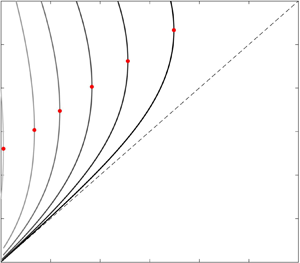
A second method was used by Camassa, Ogrosky & Olander (Reference Camassa, Ogrosky and Olander2014) for predicting plug formation in the presence of gravity-driven base flow. They found that travelling wave solution branches could be readily found for thin films; as the film thickness increased, however, a turning point in the family of solutions was reached, and beyond this point no solutions could be found. These turning points have been shown to correspond well with the critical film thickness separating plug formation from no plugs in both experiments and model simulations in a variety of models (Camassa et al. Reference Camassa, Ogrosky and Olander2014, Reference Camassa, Marzuola, Ogrosky and Vaughn2016; Ding et al. Reference Ding, Liu, Liu and Yang2019; Dietze, Lavalle & Ruyer-Quil Reference Dietze, Lavalle and Ruyer-Quil2020).
In the current paper, a long-wave model is derived to describe both thin- and thick-film flows with insoluble surfactant inside a tube in the presence or absence of base flow due to gravity, active core flow or both. The focus here will be primarily on low Reynolds number (and low capillary number and low Marangoni number) flows. In these regimes the axisymmetric dynamics is likely to play a significant if not dominant role, and thus the models developed here will assume axisymmetry. In other parameter regimes, not only may azimuthal instabilities play a leading role, but also short-wave instabilities, and the long-wave asymptotic modelling approach would likely be insufficient to capture this dynamics. Following the approach of Camassa et al. (Reference Camassa, Forest, Lee, Ogrosky and Olander2012) for flows without surfactant, the ratio of core-to-annular viscosities will be assumed to be large, and this will be exploited to decouple the core dynamics from the film dynamics; here, with surfactant included, this results in two coupled partial differential equations (PDEs), one for the free-surface evolution and one for the surfactant concentration at the film's free surface. In the absence of base flow, the effects of film thickness on the linear stability and plug formation characteristics will be studied and previous thin-film model results will be extended for thick films. In the presence of base flow, travelling wave solutions will be found and used, where possible, to identify the impact surfactant concentration has on plug formation, wave amplitude and other nonlinear features of the film flow.
The rest of the paper is organized as follows: the main model is derived in § 2. After briefly discussing solution techniques in § 3, model results in the absence of base flow are given in § 4. Results for a falling film with a passive air core are given in § 5 followed by results for core–annular flow in § 6. Conclusions are given in § 7.
2. Model development
The problem studied here is a highly viscous film with dynamic viscosity  $\bar {\mu }$ and density
  $\bar {\rho }$ that coats the interior of a rigid tube with radius
  $\bar {a}$. The core region of the tube is occupied by a much less viscous fluid, possibly air, with viscosity
  $\bar {\mu }^{(c)}\ll \bar {\mu }$ and density
  $\bar {\rho }^{(c)}$; this core fluid may either be passive or actively driven by a pressure gradient. The flow of the fluids is assumed to be axisymmetric with independent coordinates
  $(\bar {r},\bar {z})$; the positive
  $\bar {z}$-direction is up the tube so that acceleration due to gravity
  $\bar {g}$ is oriented in the negative
  $\bar {z}$ direction. The centre of the tube is at
  $\bar {r}=0$, the tube wall is at
  $\bar {r}=\bar {a}$ and the free surface lies at
  $\bar {r}=\bar {R}(\bar {z},\bar {t})$. Bars denote dimensional quantities. See figure 1 for the definition sketch of the flow variables.

Figure 1. Definition sketch of the flow variables in a vertical tube with radius  $\bar {a}$;
  $\bar {r}=\bar {R}(\bar {z},\bar {t})$ denotes the location of the free surface;
  $\bar {h}(\bar {z},\bar {t})$ denotes the film thickness;
  $\bar {R}_0$ (
 $\bar {h}_0$) denotes the mean core (film) thickness;
  $\bar {\varGamma }(\bar {z},\bar {t})$ denotes the concentration of insoluble surfactant at the free surface.
Insoluble surfactant is assumed to be present at the free surface with concentration  $\bar {\varGamma }(\bar {z},\bar {t})$ and diffuses with diffusion coefficient
  $\bar {D}_s$. The surface tension at the free surface depends on the concentration and is denoted by
  $\bar {\sigma }(\bar {\varGamma })$. A long-wave model for this flow is derived next.
2.1. Governing equations and boundary conditions
The flow of the annular film is governed by the cylindrical axisymmetric Navier–Stokes equations
 \begin{gather} \bar{\rho}(\bar{u}_{\bar{t}}+\bar{u}\bar{u}_{\bar{r}}+\bar{w}\bar{u}_{\bar{z}}) =-\bar{p}_{\bar{r}}+\bar{\mu}\left(\frac{1}{\bar{r}}\partial_{\bar{r}}(\bar{r} \bar{u}_{\bar{r}})+\bar{u}_{\bar{z}\bar{z}}-\frac{\bar{u}}{\bar{r}^{2}}\right), \end{gather}
 \begin{gather}\bar{\rho}(\bar{w}_{\bar{t}}+\bar{u}\bar{w}_{\bar{r}}+\bar{w}\bar{w}_{\bar{z}}) =-\bar{p}_{\bar{z}}+\bar{\mu}\left(\frac{1}{\bar{r}}\partial_{\bar{r}} (\bar{r}\bar{w}_{\bar{r}})+\bar{w}_{\bar{z}\bar{z}}\right)-\bar{\rho} \bar{g}, \end{gather}
 \begin{gather}\frac{1}{\bar{r}}\partial_{\bar{r}}(\bar{r}\bar{u})+\bar{w}_{\bar{z}} =0, \end{gather}
where  $(\bar {u},\bar {w})$ are the velocity components in the
  $(\bar {r},\bar {z})$ direction, respectively, and
  $\bar {p}$ is pressure. Subscripts will be used to denote partial derivatives. No-slip boundary conditions are enforced at the wall,
  $\bar {r}=\bar {a}$
 \begin{equation} \bar{w}=\bar{u}=0. \end{equation}
At the free surface,  $\bar {r}=\bar {R}$, three boundary conditions must be met: (i) continuity of tangential stress,
 \begin{equation} \frac{\bar{\mu}}{(1+(\bar{R}_{\bar{z}})^{2})}[2\bar{R}_{\bar{z}}(\bar{u}_{\bar{r}} -\bar{w}_{\bar{z}})+(1-(\bar{R}_{\bar{z}})^{2})(\bar{u}_{\bar{z}}+\bar{w}_{\bar{r}})] -\bar{\tau}^{(c)}=-\frac{1}{(1+(\bar{R}_{\bar{z}})^{2})^{1/2}}\bar{\sigma}_{\bar{z}}, \end{equation}
where  $\bar {\tau }^{(c)}$ is the tangential stress at the free surface due to active core flow; (ii) jump in normal stress according to the Young–Laplace law,
 \begin{align} &-\bar{p}+\frac{2\bar{\mu}}{(1+(\bar{R}_{\bar{z}})^{2})} [(\bar{R}_{\bar{z}})^{2}\bar{w}_{\bar{z}}-\bar{R}_{\bar{z}}(\bar{u}_{\bar{z}} +\bar{w}_{\bar{r}})+\bar{u}_{\bar{r}}]+\bar{p}^{(c)}\nonumber\\ &\quad =\frac{\bar{\sigma}(\bar{\varGamma})}{\bar{R}(1+(\bar{R}_{\bar{z}})^{2})^{1/2}} \left(1-\frac{\bar{R}\bar{R}_{\bar{z}\bar{z}}}{(1+(\bar{R}_{\bar{z}})^{2})}\right), \end{align}
where  $\bar {p}^{(c)}$ is the core fluid pressure and (iii) a kinematic boundary condition
 \begin{equation} \bar{u}=\bar{R}_{\bar{t}}+\bar{w}\bar{R}_{\bar{z}}. \end{equation}
In the case of a passive core,  $\bar {\tau }^{(c)}$ and
  $\bar {p}^{(c)}$ will be set to zero.
The surfactant flow is modelled by an advection–diffusion equation of the same form used in, e.g., Kas-Danouche et al. (Reference Kas-Danouche, Papageorgiou and Siegel2009) and Bassom et al. (Reference Bassom, Blyth and Papageorgiou2012), Zhou et al. (Reference Zhou, Peng, Zhang and Zhuge2014),
 \begin{equation} \frac{\partial}{\partial \bar{t}}[(1+(\bar{R}_{\bar{z}})^{2})^{1/2}\bar{R}\bar{\varGamma}] +\frac{\partial}{\partial \bar{z}}[\bar{w}(1+(\bar{R}_{\bar{z}})^{2})^{1/2}\bar{R}\bar{\varGamma}] =\bar{D}_s\frac{\partial}{\partial \bar{z}}\left[\frac{\bar{R} \bar{\varGamma}_{\bar{z}}}{(1+(\bar{R}_{\bar{z}})^{2})^{1/2}}\right]. \end{equation}
The dependence of surface tension  $\bar {\sigma }$ on surfactant concentration is generally nonlinear, but may be linearized about the mean concentration,
 \begin{equation} \bar{\sigma}(\bar{\varGamma})=\bar{\sigma}_0-\bar{R}^{*}\bar{T}(\bar{\varGamma}- \bar{\varGamma}_0), \end{equation}
where it has been assumed that the surfactant concentration  $\bar {\varGamma }$ is much less than the maximum packing value
  $\bar {\varGamma }_{\infty }$, and where
  $\bar {\sigma }_0$ is surface tension corresponding to the base surfactant concentration value
  $\bar {\varGamma }_0$,
  $\bar {R}^{*}$ is the universal gas constant and
  $\bar {T}$ is absolute temperature.
2.2. Scalings and dimensionless equations
Equations (2.1)–(2.7) may be made dimensionless using the following scales,
 \begin{gather} \left.\begin{gathered} r =\dfrac{\bar{r}}{\bar{R}_0},\quad z=\dfrac{\bar{z}}{\bar{\lambda}}, \quad u=\dfrac{\bar{u}}{\bar{U}_0},\quad w=\dfrac{\bar{w}}{\bar{W}_0}, \quad t=\dfrac{\bar{t}\bar{W}_0}{\bar{\lambda}},\quad p=\dfrac{\epsilon \bar{p}\bar{R}_0}{\bar{\mu}\bar{W}_0},\quad \tau=\dfrac{\bar{\tau}\bar{R}_0}{\bar{\mu}\bar{W}_0},\\ \sigma =\dfrac{\bar{\sigma}}{\bar{\sigma}_0},\quad\varGamma= \dfrac{\bar{\varGamma}}{\bar{\varGamma}_0}, \end{gathered}\right\} \end{gather}
where  $\bar {\lambda }$ is a length scale in the
  $z$-direction (corresponding to the wavelength of a typical free-surface disturbance), and where
  $\bar {U}_0$ and
  $\bar {W}_0$ are velocity scales in the
  $r$ and
  $z$ directions, respectively. The velocity scales used will depend on whether a base flow is present: in the absence of any base flow, the axial velocity scale will be taken to be
  $\bar {W}_0=\bar {\sigma }_0/\bar {\mu }$; for a falling film, the velocity scale may be taken to be the undisturbed velocity of the free surface,
  $\bar {W}_0=\bar {\rho }\bar {g}\bar {h}_0^{2}/\bar {\mu }$; for pressure-driven core–annular flow,
  $\bar {W}_0=2\bar {Q}^{(c)}/{\rm \pi} \bar {R}_0^{2}$ may be taken to be a centreline velocity with core volume flux
  $\bar {Q}^{(c)}$ as in, e.g., Camassa et al. (Reference Camassa, Forest, Lee, Ogrosky and Olander2012); Camassa & Ogrosky (Reference Camassa and Ogrosky2015). A long-wave approximation will be made, where variations in
  $\bar {z}$ will be assumed smaller than variations in
  $\bar {r}$, so that
  $\epsilon =\bar {R}_0/\bar {\lambda }\ll 1$ (and
  $\bar {U}_0=\epsilon \bar {W}_0$). We note that other scaling options could be used as well. A thin-film approximation exploiting an assumed small ratio of film thickness to tube radius would be suitable here, though a long-wave model may be able to shed light on the dynamics when the film is not thin. It is important to note that each modelling approach may capture different physics; as one of the goals of the current study is to study thick films and plug formation, the thin-film approach is not used here. The dimensionless parameters that appear in the equations and boundary conditions,
 \begin{align} Re=\frac{\bar{\rho}\bar{W}_0\bar{R}_0}{\bar{\mu}},\quad Fr=\frac{\bar{W}_0}{\sqrt{\bar{g}\bar{R}_0}},\quad C=\frac{\bar{\mu}{\bar{W}_0}}{\bar{\sigma}_0},\quad M=\frac{\bar{R}\bar{T}\bar{\varGamma}_0}{\bar{\sigma}_0},\quad Pe=\frac{\bar{W}_0\bar{R}_0}{\bar{D}_s},\quad a=\frac{\bar{a}}{\bar{R}_0}, \end{align}
are the Reynolds, Froude, capillary, Marangoni and Péclet numbers, and a film thickness parameter  $a$, respectively. The film thickness parameter may be rewritten in terms of dimensionless film thickness
  $h_0=\bar {h}_0/\bar {a}$ through
  $a=1/(1-h_0)$. The domain of
  $a$ is
  $(1,\infty )$ (and for
  $h_0$ is (0,1)) with
  $a\rightarrow 1$ (
 $h_0\rightarrow 0$) corresponding to the limit of the core fluid filling the entire tube, and
  $a\rightarrow \infty$ (
 $h_0\rightarrow 1$) corresponding to the limit of the annular fluid filling the entire tube.
Throughout the derivation, the Reynolds number will be assumed to be small; as a result,  $O(\epsilon Re)$ terms will not be retained, but
  $O(\epsilon )$ terms will. The Marangoni number will also be assumed to be small, as discussed in, e.g., Frenkel & Halpern (Reference Frenkel and Halpern2017).
The dimensionless momentum equations and boundary conditions using (2.8) are given in appendix A, (A 1)–(A 6). When only terms of  $O(1)$ and
  $O(\epsilon )$ are retained, the resulting momentum equations are
 \begin{gather} p_r =0, \end{gather}
 \begin{gather}p_z =\frac{1}{r}\partial_r(rw_r)-\frac{Re}{Fr^{2}}-\epsilon Re(w_t+uw_r+ww_z), \end{gather}
 \begin{gather}\frac{1}{r}\partial_r(ru)+w_z =0. \end{gather}
The dimensionless boundary conditions are no slip at the wall,  $r=a$,
 \begin{equation} u=w=0. \end{equation}
At the free surface,  $r=R$, the three boundary conditions are
 \begin{gather} w_r-\tau_c =\frac{\epsilon M}{C}\varGamma_z, \end{gather}
 \begin{gather}-p^{(a)}+p^{(c)} =\frac{\epsilon}{C}[1-M(\varGamma-1)] \left(\frac{1}{R}-\epsilon^{2}R_{zz}\right), \end{gather}
 \begin{gather}u =R_t+wR_z. \end{gather}
Note that (2.12b) has one term of  $O(\epsilon ^{3})$. This term has been retained for several reasons and is also retained in many other film flow models derived using long-wave asymptotics. For one, this term has been shown in previous studies to be the lowest-order one in the long-wave asymptotics that prevents shock formation, providing some rationale for retention of this term and exclusion of other terms of comparable or higher order. For another, this term provides the correct upper bound on unstable wavenumbers in the case of a clean interface.
There is no guarantee that the resulting competition in the model between the destabilizing terms of  $O(\epsilon )$ and stabilizing term of
  $O(\epsilon ^{3})$ will be a faithful representation of the dynamics in the full equations since the range of unstable wavenumbers will extend well outside the
  $k\ll 1$ range. However, a comparison between the model's dispersion relation and previous linear stability results for the full Stokes equations (Zhou et al. Reference Zhou, Peng, Zhang and Zhuge2014) suggests the model is reasonably effective at reproducing the full dispersion relation, and we note here that asymptotic models, particularly long-wave models derived in this way, have been previously applied outside their range of validity and found to be in good agreement with moderately thick-film experiments (e.g., Craster & Matar Reference Craster and Matar2006; Camassa et al. Reference Camassa, Ogrosky and Olander2014).
The linearized dimensionless constitutive equation is
 \begin{equation} \sigma=1-M(\varGamma-1), \end{equation}
and the dimensionless advection–diffusion equation for surfactant is
 \begin{equation} [R\varGamma]_t+[wR\varGamma]_z=\frac{\epsilon}{Pe}[R\varGamma_z]_z. \end{equation}
The continuity equation may be integrated across the annular fluid layer; using the kinematic boundary condition produces
 \begin{equation} \left(\frac{R^{2}}{2}\right)_t=\left[\int_R^{a}wr\, \textrm{d} r\right]_z. \end{equation}
 Equations (2.14) and (2.15) form the long-wave model and are conservation laws with conserved quantities  $R\varGamma$ and
  $R^{2}$, respectively. An approximate expression for
  $w$ is needed to close the system, and can be found by solving (2.10)–(2.12) assuming a regular perturbation expansion,
 \begin{equation} \left. \begin{gathered} w=w_0+\epsilon w_1+O(\epsilon^{2}),\\ u=u_0+\epsilon u_1+O(\epsilon^{2}),\\ p=p_0+\epsilon p_1+O(\epsilon^{2}). \end{gathered}\right\} \end{equation}
Solving the equations at  $O(1)$ gives
 \begin{equation} w_0=\frac{(r^{2}-a^{2})}{4}\left(p_z+\frac{Re}{Fr^{2}}\right)+ \left(R\tau^{(c)}-\frac{R^{2}}{2}\left(p_z+\frac{Re}{Fr^{2}}\right)\right) \log\frac{r}{a}.\end{equation}
The pressure gradient  $p_z$ is independent of
  $r$ but depends on
  $p_z^{(c)}$ through (2.12b). In the case of a passive core, as with a falling film in a vertical tube, both
  $\tau ^{(c)}$ and
  $p_z^{(c)}$ may be set to zero, but in the case of active core flow, estimates of both
  $\tau ^{(c)}$ and
  $p_z^{(c)}$ are needed. One way to estimate
  $\tau ^{(c)}$ and
  $p^{(c)}_z$ is to use the locally Poiseuille model of Camassa et al. (Reference Camassa, Forest, Lee, Ogrosky and Olander2012), which produces
 \begin{gather} p_z^{(c)} =-\frac{\bar{\rho}^{(c)}}{\bar{\rho}}\frac{Re}{Fr^{2}}-\frac{4}{m\,R^{4}}, \end{gather}
 \begin{gather}\tau^{(c)} =-\frac{2}{m\,R^{3}}, \end{gather}
where  $m=\bar {\mu }/\bar {\mu }^{(c)}$ is the viscosity ratio. These estimates arise from finding a steady solution to Poiseuille flow of the core fluid through a pipe with radius
  $R$, and is valid when
  $\bar {\mu }^{(c)}\ll \bar {\mu }$ so that the core flow can be decoupled from the film flow (see Camassa & Ogrosky (Reference Camassa and Ogrosky2015) for further details). Other modelling approaches that make use of this decoupling in pipe or channel flow could be used as well, such as the models of Tseluiko & Kalliadasis (Reference Tseluiko and Kalliadasis2011) or Camassa, Ogrosky & Olander (Reference Camassa, Ogrosky and Olander2017).
The derivation used here, and in previous modelling studies employing this ‘locally Poiseuille’ approach, neglects the effects of instability due to viscosity stratification and is only valid for viscous films where the effects due to surface tension are dominant. For flows with moderate Reynolds number, or for flows with weak surface tension, one may expect that the effects of viscosity stratification will become significant and the model derived here may not be expected to apply. Both weakly and strongly nonlinear thin-film models have been previously derived with these effects, which typically enter into the model as a non-local term due to the core flow being readily solved in Fourier space; see, e.g., Papageorgiou et al. (Reference Papageorgiou, Maldarelli and Rumschitzki1990), Georgiou et al. (Reference Georgiou, Maldarelli, Papageorgiou and Rumschitzki1992), Kas-Danouche et al. (Reference Kas-Danouche, Papageorgiou and Siegel2009) and Dietze & Ruyer-Quil (Reference Dietze and Ruyer-Quil2015), among others. For examples of models that, like the one developed here, also neglect this instability due to viscosity stratification, see, e.g., Frenkel et al. (Reference Frenkel, Babchin, Levich, Shlang and Sivashinsky1987), Kerchman (Reference Kerchman1995), Wei & Rumschitzki (Reference Wei and Rumschitzki2005), Camassa et al. (Reference Camassa, Forest, Lee, Ogrosky and Olander2012), etc. It is in this vein, particularly that of Camassa et al. (Reference Camassa, Forest, Lee, Ogrosky and Olander2012), that the model derivation here proceeds, and in the case of equal density fluids and no surfactant, the model developed here reduces to that of Kerchman (Reference Kerchman1995) in the thin-film limit. Details of the model derivation calculations are given in appendix A; see also Camassa & Ogrosky (Reference Camassa and Ogrosky2015).
Next, proceeding to  $O(\epsilon )$ and solving equations (2.10)–(2.12) for
  $w_1$ produces
 \begin{align} w_1=-\frac{1}{4C}\left[(1-M(\varGamma-1))\left(\frac{1}{R}-R_{zz}\right)\right]_z \left(r^{2}-a^{2}-2R^{2}\log\frac{r}{a}\right)+\frac{RM\varGamma_z}{C}\log\frac{r}{a},\end{align}
where terms of  $O(\epsilon Re)$ have been neglected due to the assumed small Reynolds number. Substituting the total velocity
  $w=w_0+\epsilon w_1$ into (2.15) produces
 \begin{align} R_t&=-\left[S_1\,f_1(R;a)+\frac{\tilde{S}_2}{a^{4}}\,f_2(R;a)\right]R_z +{\frac{4M\tilde{S}_3}{a^{2}R}[R\varGamma_z\,\,f_2(R;a)]_z}\nonumber\\ &\quad-\frac{\tilde{S}_3}{a^{2}R}[[{M\varGamma_z (R-R^{2}R_{zz})}+(1-{M(\varGamma-1)})(R_z+R^{2}R_{zzz})]\,f_3(R;a)]_z, \\[-2.5pc]\nonumber\end{align}
 \begin{equation} \varGamma_t=-\frac{\varGamma}{R}R_t-\frac{1}{R}[R\varGamma w(R)]_z+\frac{1}{{a}\,\widetilde{Pe}\,R}[R_z\varGamma_z+R\varGamma_{zz}],\end{equation}
where  $\epsilon$ has been scaled out of the model by returning to the original aspect ratio through a rescaling of
  $z$ and
  $t$ (see, e.g., Camassa & Ogrosky Reference Camassa and Ogrosky2015). There are six model parameters; film thickness parameter
  $a$ (or alternately
  $h_0=1-1/a$), Marangoni number
  $M$ and
 \begin{equation} S_1=\frac{1}{m},\quad \tilde{S}_2=\frac{a^{4}(\bar{\rho}-\bar{\rho}^{(c)})Re}{2\bar{\rho}Fr^{2}},\quad \tilde{S}_3=\frac{a^{2}}{16C}, \quad \widetilde{Pe}=a\,Pe, \end{equation}
with  $f_i$ values
 \begin{gather} f_1(R;a) =\frac{a^{2}}{R^{4}}\left(\frac{a^{2}}{R^{2}}-1\right), \end{gather}
 \begin{gather} f_2(R;a)=R^{2}-a^{2}-2R^{2}\log\frac{R}{a}, \end{gather}
 \begin{gather} f_3(R;a)=\frac{a^{4}}{R^{2}}-4a^{2}+3R^{2}-4R^{2}\log\frac{R}{a}, \end{gather}
and with velocity at the free surface in (2.20b) of
 \begin{align} w(R)&= \frac{S_1R^{2}}{a^{2}}\,f_1(R;a)+{\frac{16M\tilde{S}_3}{a^{2}}\varGamma_zR\log\frac{R}{a}}\nonumber\\ &\quad +\left[\frac{\tilde{S}_2}{2a^{4}}+\frac{4\tilde{S}_3}{a^{2}} \left[M\varGamma_z\left(\frac{1}{R}-R_{zz}\right)+(1-M(\varGamma-1)) \left(\frac{R_z}{R^{2}}+R_{zzz}\right)\right]\right]\,f_2(R;a). \end{align}
2.3. Model subcases
Before proceeding to solutions of (2.20), three special cases of (2.20a) that will be the focus of the rest of the paper are written out explicitly for reference. In the case of a passive air core and viscous film in a capillary with no base flow, i.e.  $S_1=\tilde {S}_2=0$, the velocity scale may be taken as
  $\bar {W}_0=\bar {\sigma }_0/\bar {\mu }$ so that
  $\tilde {S}_3=1/16$; (2.20a) is then
 \begin{align} R_t&= {\frac{M}{4a^{2}R} [R\varGamma_z\,f_2(R;a) ]_z}\nonumber\\ &\quad-\frac{1}{16a^{2}R} [ [{M\varGamma_z (R-R^{2}R_{zz} )} + (1-{M(\varGamma-1)} ) (R_z+R^{2}R_{zzz} ) ]\,f_3(R;a) ]_z, \end{align}
with  $M$,
$M$,  $a$ and
  $\widetilde {Pe}$ the model parameters. Equations (2.24) and (2.20b) are similar to the model developed in Halpern & Grotberg (Reference Halpern and Grotberg1993) for the case of a rigid tube wall, but it retains more of the cylindrical geometry of the problem, including conserving
  $R\varGamma$ rather than
  $\varGamma$. The model used here is also similar to that of Otis et al. (Reference Otis, Johnson, Pedley and Kamm1993), although their model uses an empirical surfactant equation of state. In the absence of surfactant, the model used here reduces in the thin-film limit to that derived by Hammond (Reference Hammond1983) and studied by Lister et al. (Reference Lister, Rallison, King, Cummings and Jensen2006).
In the case of a falling viscous film in a vertical tube (with a passive air core), we may take  $S_1=0$ and rescale in time by
  $\tilde {S}_2$ to get
 \begin{align} R_t&=-\left[\frac{1}{a^{4}}\,f_2(R;a)\right]R_z+{\frac{4M}{a^{2}\,Bo\,R} [R\varGamma_z\,f_2(R;a) ]_z}\nonumber\\ &\quad-\frac{1}{a^{2}\,Bo\,R} [ [{M\varGamma_z (R-R^{2}R_{zz} )}+ (1-{M(\varGamma-1)} ) (R_z+R^{2}R_{zzz} ) ]\,f_3(R;a) ]_z, \end{align}
with  $M$,
$M$,  $a$,
$a$,  $\widetilde {Pe}$ and
  $Bo$ the model parameters;
  $Bo$ is a Bond number defined as
 \begin{equation} Bo=\frac{\tilde{S}_2}{\tilde{S}_3}=\frac{8\bar{a}^{2}(\bar{\rho}- \bar{\rho}^{(c)})g}{\bar{\sigma}_0}\approx\frac{8\bar{\rho}\bar{g}\bar{a}^{2}}{\bar{\sigma}_0}, \end{equation}
where the approximation holds when  $\bar {\rho }^{(c)}\ll \bar {\rho }$, as with a liquid annular film and air in the core region. Note that
  $Bo$ does not depend on the film thickness, and has been defined in terms of ‘hardware’ parameters only, i.e. properties of the fluid and the dimensional tube radius. In the absence of surfactant, the model here was studied by Camassa et al. (Reference Camassa, Ogrosky and Olander2014) and is similar to the model derived by Lin & Liu (Reference Lin and Liu1975). It is also the interior counterpart to the models of Craster & Matar (Reference Craster and Matar2006) and Kliakhandler, Davis & Bankoff (Reference Kliakhandler, Davis and Bankoff2001) who studied gravity-driven film flow down the exterior of a tube; this exterior model compared well with experiments by Smolka, North & Guerra (Reference Smolka, North and Guerra2008). In the thin-film limit, the mode here reduces to that of Frenkel (Reference Frenkel1992) that was studied by Kerchman & Frenkel (Reference Kerchman and Frenkel1994) and Kalliadasis & Chang (Reference Kalliadasis and Chang1994); plug formation in this model was also studied by Jensen (Reference Jensen2000).
In the case of core–annular flow with matching densities, i.e.  $\tilde {S}_2=0$ so that effects of gravity are neglected, the model may be rescaled in time by
  $S_1$
$S_1$
 \begin{align} R_t&=-\,f_1(R;a)R_z+{\frac{M}{4a^{2}R\,\tilde{C}} [R\varGamma_z\,f_2(R;a) ]_z}\nonumber\\ &\quad-\frac{1}{a^{2}R\,\tilde{C}} [ [{M\varGamma_z (R-R^{2}R_{zz} )}+ (1-{M(\varGamma-1)} ) (R_z+R^{2}R_{zzz} ) ]\,f_3(R;a) ]_z, \end{align}
where  $\tilde {C}=16C/m$ is a modified Capillary number; parameters
  $M$,
$M$,  $a$ and
  $\tilde {C}$ determine the dynamics (again assuming large Péclet number). In the absence of surfactant, the model here was studied by Camassa & Ogrosky (Reference Camassa and Ogrosky2015) and it reduces to the model by Kerchman (Reference Kerchman1995) in the thin-film limit. We note that the model derivation assumes small Reynolds number, and that the effects of surface tension are significantly larger than instability due to viscosity stratification so that the latter may be neglected. In parameter regimes where these assumptions are not valid, the model cannot be expected to accurately represent the dynamics.
3. Solution methods
Before presenting results, analytical and numerical solution methods are briefly discussed.
3.1. Linear stability
The linear stability of constant solutions to the long-wave model may be studied by adding a small-amplitude sinusoidal perturbation with wavenumber  $k$ to the undisturbed base state
  $R(z,t)=\varGamma (z,t)=1$; i.e.
 \begin{equation} R=1+\hat{R}\,\textrm{e}^{\textrm{i}(kz-\omega t)},\quad \varGamma=1+\hat{\varGamma}\,\textrm{e}^{\textrm{i}(kz-\omega t)}, \end{equation}
with  $\hat {R}\ll 1$ and
  $\hat {\varGamma }\ll 1$. Substitution of (3.1a,b) into (2.20) results in an eigenvalue problem for
  $\omega$,
 \begin{equation} (\boldsymbol{A}-\textrm{i}\omega I)(\hat{R},\hat{\varGamma})^\textrm{T}=0. \end{equation}
The elements of  $\boldsymbol {A}$ are
 \begin{equation} a_{11} =\left[S_1\,f_1(1;a)+\frac{\tilde{S}_2}{a^{4}}\,f_2(1;a)\right]ik+ \frac{\tilde{S}_3}{a^{2}}\,f_3(1;a)(k^{4}-k^{2}), \end{equation}
 \begin{equation}a_{12} =\frac{M\tilde{S}_3}{a^{2}}[4\,f_2(1;a)-\,f_3(1;a)]k^{2}, \end{equation}
 \begin{align} a_{21}&=\left[-S_1\,f_1(1;a)-\frac{\tilde{S}_2}{a^{4}}\,f_2(1;a) +\frac{S_1\,f_4(1;a)}{a^{2}}+\frac{\tilde{S}_2\,f_5(1;a)}{2a^{4}}+w_R\right]ik\nonumber\\ &\quad+\frac{\tilde{S}_3}{a^{2}}[4\,f_2(1;a)-\,f_3(1;a)](k^{4}-k^{2}), \end{align}
 \begin{equation} a_{22}=w_Rik+\left[\frac{M\tilde{S}_3}{a^{2}}\,f_3(1;a)+ \frac{1}{a\widetilde{Pe}}+\frac{4M\tilde{S}_3\,f_5(1;a)}{a^{2}}- \frac{8M\tilde{S}_3\,f_2(1;a)}{a^{2}}\right]k^{2}, \end{equation}
and
 \begin{gather} f_1(1;a) =a^{4}-a^{2}, \end{gather}
 \begin{gather}f_2(1;a) =1-a^{2}+2\log a, \end{gather}
 \begin{gather}f_3(1;a) =a^{4}-4a^{2}+3+4\log a, \end{gather}
 \begin{gather}f_4(1;a) =-4a^{4}+2a^{2}, \end{gather}
 \begin{gather}f_5(1;a) =4\log a, \end{gather}
 \begin{gather}w_R =\frac{S_1\,f_1(1;a)}{a^{2}}+\frac{\tilde{S}_2\,f_2(1;a)}{2a^{4}}, \end{gather}
with  $w_R$ the fluid velocity at the free surface. Solving (3.2) results in a quadratic equation for
  $\omega$. When
  $M=0$, one of these roots is identical to the dispersion relation for a clean-interface version of the model and is thus sometimes referred to as the interface mode (even though this mode may consist of
  $\varGamma$ perturbations as well as
  $R$ perturbations). As
  $M$ is increased, this interface mode may be expected to be modified as surfactant perturbations are fully coupled to the interfacial evolution. The second mode consists only of surfactant perturbations when
  $M=0$, and is thus sometimes termed the ‘surfactant’ mode; for
  $M>0$, typically both
  $R$ and
  $\varGamma$ perturbations are present in the surfactant mode as well. This terminology will be adopted here as well. The distinction between the two modes can become blurred as parameters vary (particularly in the case of a base flow); nevertheless this terminology will be adopted for the rest of the paper and in most cases reported here is fairly unambiguous. Other terminology used in the literature includes the ‘robust mode’ and ‘surfactant mode’ as in, e.g., Frenkel & Halpern (Reference Frenkel and Halpern2017), who note that the robust mode, like the interface mode, does not vanish as
  $M\rightarrow 0$; see, e.g., Frenkel et al. (Reference Frenkel, Halpern and Schweiger2019a) for use of this terminology and discussion of the mode branches in a planar geometry case with base flow.
It is important to note that the long-wave model was derived under the assumption of aspect ratio  $\epsilon =\bar {R}_0/\bar {\lambda }\ll 1$, and so this linear stability analysis conducted on the model should be a faithful representation of the full system's linear dynamics in the limit
  $k\rightarrow 0$ (in the parameter regimes considered here). However, in the linear stability analysis conducted here, all terms in the model equations are retained and their impacts on the growth rates taken into account, regardless of order, as has been done in other studies of long-wave film flow models. This includes stabilizing terms of
  $O(k^{4})$ that arise due to the axial free-surface curvature, and that introduce both a wavenumber of maximum growth rate (
 $k_{max}$) and a cutoff wavenumber which lie outside the model's region of validity. They will be shown, however, to be in good agreement with those of the full Stokes equations found by Zhou et al. (Reference Zhou, Peng, Zhang and Zhuge2014). It is important to remember, however, that in the long-wave limit and with the approximations made here, those terms of
  $O(k^{2})$ are the dominant terms in determining growth rates.
3.2. Numerical methods
Approximate solutions to the nonlinear model equations will be found numerically using periodic boundary conditions. Each equation is integrated using a pseudospectral method; i.e. spatial derivatives are calculated in Fourier space while nonlinearities are calculated in physical space. Dealiasing is applied at each time step due to the complicated nonlinearities in the model. The time integration scheme is a simple second-order predictor–corrector scheme. As both  $R^{2}$ and
  $R\varGamma$ are conserved quantities in (2.20), these values are monitored throughout the simulations, and simulations are repeated with finer spatial or temporal resolution if necessary. The initial conditions used are a flat free surface perturbed with one or more Fourier modes:
  $R(z,t)=1+\sum _{k=1}^{n}a_k\cos (2{\rm \pi} kz +b_k)$, where
  $b_k$ is a random phase shift, and
  $\varGamma (z,t)=1+\sum _{k=1}^{n}\tilde {a}_k\cos (2{\rm \pi} kz +\tilde {b}_k)$. In some simulations
  $\tilde {a}_k=\tilde {b}_k=0$ so that a perfectly even distribution of surfactant is assumed at
  $t=0$; the long-time evolution of the system was not typically found to depend strongly on these values of
  $a_k,b_k,\tilde {a}_k,\tilde {b}_k$. The nonlinear code was tested through convergence tests as well as running simulations using initial conditions consisting of an undisturbed
  $R$ and
  $\varGamma$ plus small-amplitude linear eigenmodes; the evolution of these eigenmodes for early times was checked against the linear stability analysis results to ensure proper propagation and growth/decay.
Travelling wave solutions, i.e. solutions to the model equations of the form  $R(z,t)^{2}=Q(z-ct)$,
  $R(z,t)\varGamma (z,t)=N(z-ct)$, will also be sought. Since (2.20) is a conservation law, each equation may be integrated once, resulting in two constants of integration
  $K_1$ and
  $K_2$. The resulting system consisting of one third-order ordinary differential equation (ODE) and one first-order ODE may then be rewritten as a system of four first-order ODEs and solved using standard numerical methods. The approach used here mimics the one described in Camassa et al. (Reference Camassa, Marzuola, Ogrosky and Vaughn2016). Briefly, the model has a family of constant solutions
  $R(z,t)=R_0$ and
  $\varGamma (z,t)=\varGamma _0$ with
  $R_0,\varGamma _0$ depending on model parameters (including constants of integration
  $K_1$ and
  $K_2$). Continuing along this family of solutions results in a Hopf bifurcation (or zero-Hopf bifurcation, in which case a small smoothing term may be added to make numerical continuation onto the family of periodic solutions easier; see Camassa et al. (Reference Camassa, Marzuola, Ogrosky and Vaughn2016) for details). The continuation software AUTO (Doedel et al. Reference Doedel, Champneys, Dercole, Fairgrieve, Kuznetsov, Oldeman, Paffenroth, Sandstede, Wang and Zhang2008Reference Duprat, Ruyer-Quil, Kalliadasis and Giorgiutti-Dauphine) was used to find the Hopf bifurcation and subsequent periodic solutions. In all results shown here, integral conditions
  $(1/T)\int _0^\textrm {T}R^{2}\, \textrm {d} z=(1/T)\int _0^\textrm {T}R\varGamma \, \textrm {d} z=1$ were enforced (where
  $T$ is the period).
4. Results for no base flow
Model results are presented first for the case of a passive core and viscous film in a capillary with no base flow (i.e.  $S_1=\tilde {S}_2=0$) studied by Hammond (Reference Hammond1983), Otis et al. (Reference Otis, Johnson, Pedley and Kamm1993) and Halpern & Grotberg (Reference Halpern and Grotberg1993) and others. Results with base flow due either to gravity or core flow are given in the following sections. In common with many other studies of film flows in the presence of surfactant, the Péclet number is assumed to be large in all results presented here, with
  $\widetilde {Pe}=10^{4}$ or larger; in some results diffusion will be neglected altogether.
4.1. Linear stability analysis
In this case the free surface and surfactant concentration are governed by (2.24) and (2.20b). Aside from the (large) Péclet number, the two parameters governing the dynamics are film thickness parameter  $a$ and Marangoni number
  $M$. The linear modes are shown in figure 2(c,d) for
  $M=0.1$,
  $a=2$, and
  $k=0.7$, and the growth rates for modes with a variety of
  $M$ values for
  $a=1.11$ and
  $a=2$ are shown in figure 2(a,b). Both eigenmodes contain perturbations to
  $R$ and to
  $\varGamma$ that are in phase with one another due to the lack of a base flow. In the case
  $M=0$, the surfactant mode contains only disturbances to surfactant concentration; the interface mode contains both perturbations to
  $R$ and
  $\varGamma$.

Figure 2. (a,b) Growth rates for the unstable mode in (2.24) and (2.20b) with no base flow for various values of  $M$;
$M$;  $S_1=\tilde {S}_2=0$,
  $\tilde {S}_3=1/16$,
  $\widetilde {Pe}=10^{5}$: (a)
  $a=1.11$ (
 $h_0=0.1$); (b)
  $a=2$ (
 $h_0=0.5$). (c,d) Linear eigenmodes for
  $M=0.1$,
  $S_1=\tilde {S}_2=0$,
  $\tilde {S}_3=1/16$,
  $k=0.7$,
  $a=2$ (
 $h_0=0.5$).
For all combinations of  $a$ and
  $M$, the only unstable mode is the interface mode. Figure 2 shows the growth rates of this mode for various values of
  $M$ and
  $a$. For
  $M=0$, the wavenumber of maximum growth rate is
  $k_{max}=1/\sqrt {2}$ as expected (Hammond Reference Hammond1983; Halpern & Grotberg Reference Halpern and Grotberg1993). As
  $M$ increases,
  $k_{max}$ decreases slightly, and then increases until returning to
  $1/\sqrt {2}$ in the limit
  $M\rightarrow \infty$. For all values of
  $a$ and
  $M$, wavenumbers
  $0<k<1$ are unstable, with all larger wavenumbers stable. The smallest value that
  $k_{max}$ can attain for a particular value of
  $a$ decreases as
  $a$ increases; i.e. for thicker films, moderate values of
  $M$ result in a greater change to the dominant wavelength.
Figure 3(a) shows the ratio of the maximum growth rates  $GR_M$ (solid lines) for various values of
  $M$ and
  $GR_0$, the maximum growth rate for
  $M=0$, for three values of
  $a$. For each fixed value of
  $a$, the growth rate ratio
  $GR_0/GR_M$ increases as
  $M$ increases, with noticeable increases occurring at smaller
  $M$ for thinner films. As
  $M\rightarrow \infty$, the maximum growth rate approaches a value
  $GR_{\infty }$ which is a fraction of
  $GR_0$. For thin films, it has been shown by Halpern & Grotberg (Reference Halpern and Grotberg1993) and others that
  $GR_{0}/GR_{\infty }=4$. The long-wave model here produces a ratio
  $GR_0/GR_{\infty }$ that appears to be just greater than 4 for
  $a=1.11$ (
 $h_0=0.1$), in good agreement with these earlier results obtained with thin-film models. As
  $a$ increases, however, this ratio
  $GR_{0}/GR_{\infty }$ is significantly greater than 4, consistent with (non-long-wave) linear stability results in Zhou et al. (Reference Zhou, Peng, Zhang and Zhuge2014). This ratio can be found analytically as a function of film thickness parameter
  $a$; the growth rate of the dominant mode found by solving the eigenvalue problem (3.2) with
  $S_1=\tilde {S}_2=0$,
  $\tilde {S}_3=1/16$,
  $M=0$ (and
  $1/\widetilde {Pe}=0$ for simplicity) is
 \begin{equation} GR_0=-\frac{f_3(a)(k^{4}-k^{2})}{16a^{2}}. \end{equation}
For large  $M$, the eigenvalues may be expanded in powers of
  $1/M$; the eigenvalue corresponding to the interface mode is
  $O(1)$ and positive for
  $0<k<1$,
 \begin{equation} GR_{\infty}=\frac{(1-a^{2})[1-a^{2}+(1+a^{2})\log a](k^{4}-k^{2})}{a^{2}(a^{4}+4a^{2}-5+4\log a)}. \end{equation}
The ratio of these two interface mode eigenvalues is
 \begin{align} \frac{GR_{0}}{GR_{\infty}} &=\frac{(a^{4}-4a^{2}+3+4\log a)(a^{4}+4a^{2}-5+4\log a)}{16(a^{2}-1)[1-a^{2}+(1+a^{2})\log a]}\nonumber\\ &=4+2h_0+O(h_0^{2}). \end{align}
The top line in (4.3) gives the ratio for arbitrary film thickness parameter  $a$ using the long-wave model; the bottom expression gives the same ratio expanded in powers of
  $h_0$ in order to make an direct comparison with previous results obtained using thin-film models (Halpern & Grotberg Reference Halpern and Grotberg1993). Figure 3(b) plots this ratio as a function of
  $a$. Note that (4.3) is independent of
  $k$, consistent with each panel of figure 2 and figure 3(a).

Figure 3. (a) (Solid lines) Growth rate ratio  $GR_0/GR_M$ for various
  $M$ and
  $a$;
$a$;  $S_1=\tilde {S}_2=0$,
  $\tilde {S}_3=1/16$,
  $\widetilde {Pe}=10^{5}$. Symbols indicate closure time ratios
  $t^{*}_{M}/t^{*}_0$, and dashed lines indicate limiting growth rate ratio
  $GR_0/GR_{\infty}$. (b) Limiting growth rate ratio
  $GR_0/GR_{\infty }$ as a function of
  $a$; symbols correspond to values from panel (a). (c) Growth rate ratio
  $GR_0/GR_M$ in (4.3) as a function of
  $a$ for various fixed
  $M$.
$M$.
For fixed  $M\lesssim 0.1$, figure 3 shows that the growth rate ratio
  $GR_0/GR_M$ is actually larger for
  $a=1.11$ (
 $h_0=0.1$) than for
  $a=2$ (
 $h_0=0.5$). In other words, the relative impact of dilute surfactant on growth rate can actually be more pronounced on thin films than on thicker films. Figure 3(c) shows the growth rate ratio
  $GR_0/GR_M$ for four values of
  $M$ over the entire range of possible film thickness values. For
  $M<0.1$, after a quick increase in growth rate ratio as the film thickness increases, the growth rate ratio decreases with increasing
  $h_0$.
4.2. Nonlinear dynamics
To explore the saturation of these linear instabilities, (2.24) and (2.20b) were solved numerically. Similar to previous studies of related models (Otis et al. Reference Otis, Johnson, Pedley and Kamm1993), a domain was chosen that closely matches  $k_{max}$ in order to explore the behaviour of the most dangerous wavenumber. Once free-surface perturbations have grown beyond the linear regime, one of two main types of behaviour is seen in model solutions; either the instabilities saturate or the minimum value of
  $R$ approaches 0 rapidly. Gauglitz & Radke (Reference Gauglitz and Radke1988) identified a critical film thickness
  $h_c\approx 0.12$ for
  $M=0$ beyond which plugs may be expected to form; Halpern & Grotberg (Reference Halpern and Grotberg1993) found that increasing
  $M$ increased
  $h_c$. Both Halpern & Grotberg (Reference Halpern and Grotberg1993) and Otis et al. (Reference Otis, Johnson, Pedley and Kamm1993) quantified the time that it took for simulations to result in closure, i.e. plug formation. Halpern & Grotberg (Reference Halpern and Grotberg1993), working with a thin-film model, allowed solutions to be computed until the minimum value of
  $R$ reached 0.4 times the dimensionless tube radius
  $a$; this time was used as a proxy as the closure time, since in many simulations the minimum value of
  $R$ decreases very rapidly from
  $0.4a$ towards 0. It was found that it took roughly four times as long for films with large surfactant concentration to form plugs as surfactant-free films, mirroring the growth rate ratio found using linear stability analysis. Likewise, Otis et al. (Reference Otis, Johnson, Pedley and Kamm1993) found the closure time to approach a value slightly larger than 4 for
  $h_0=0.2$.
The same behaviour is seen in solutions to (2.24) and (2.20b). The symbols in figure 3 show the closure time ratios calculated using (2.24); these times were calculated in the same way as Halpern & Grotberg (Reference Halpern and Grotberg1993), so that once the free surface reached a value of  $0.4a$, the simulation was stopped. No plugs form for
  $h_0=0.1$ (
 $a=1.11$); for thicker films, the closure time ratios are nearly identical, or just smaller than, the growth rate ratios. Of course, it is important to note that while thick films with large
  $M$ can result in a large reduction factor in the closure time relative to that for a clean interface, the closure times themselves are much smaller than for thin films; i.e. closure happens quite rapidly with relatively thick films. It is interesting to note that the trend of decreasing
  $GR_0/GR_M$ for fixed small
  $M$ as the film thickness increases matches the trend in plug formation found in experiments by Cassidy et al. (Reference Cassidy, Halpern, Ressler and Grotberg1999); for fixed mean surfactant concentration, as the film thickens, the growth rate ratio decreased.
5. Results for gravity-driven film flow
Next the case of a falling film and passive air core in a vertical tube ( $S_1=0$,
  $\tilde {S}_2\ne 0$) is considered. Equations (2.25) and (2.20b) model this scenario, and the parameters determining the dynamics, aside from
  $\widetilde {Pe}$ which is assumed to be very large, are
  $Bo$,
$Bo$,  $M$ and
  $a$.
$a$.
5.1. Linear stability analysis
Solving the eigenvalue problem (3.2) with  $S_1=0$ (and after rescaling by
  $\tilde {S}_3$) results in two eigenmodes; for
  $M=0$, one of the modes has a dispersion relation identical to the clean-interface case, and one is a surfactant mode that is stable for all wavenumbers. The growth rate for the clean-interface mode is proportional to
  $Bo^{-1}$:
  $GR_0=\,f_3(a)(k^{2}-k^{4})/(a^{2}Bo)$.
Figure 4(a) shows the growth rates for  $a=1.11$ (
 $h_0=0.1$), and
  $Bo=1$, for various values of
  $M$. As
  $M$ increases, the interface mode's growth rates decrease; both
  $k_{max}$ (wavenumber of maximum growth rate) and the upper bound for unstable wavenumbers decrease as
  $M$ increases. Once
  $M$ has increased sufficiently, this interface mode is stable for all wavenumbers, e.g.
  $M=0.1$. The surfactant mode undergoes the opposite effect; in contrast to the case of no base flow, increasing
  $M$ increases the growth rates. As
  $M$ increases, the wavenumber of maximum growth rate for this mode goes from approximately 1 for very small
  $M$ down to approximately to
  $k=1/\sqrt {2}$ for
  $M=0.01$. Near
  $M=0.003$, the most unstable mode switches from being the interfacial mode to the surfactant mode (with higher
  $k_{max}$) as
  $M$ increases. As noted earlier, the model is only strictly valid for
  $k\ll 1$; we note here that since the cutoff wavenumber for the interface mode decreases as
  $M$ increases, perhaps the model can meet this criterion for a sufficiently large value of
  $M$ under which the cutoff wavenumber can be made small.

Figure 4. (a) Linear growth rates for (2.25) and (2.20b) with  $a=1.11$,
  $Bo=1$ and various values of
  $M$. (b,c) Linear eigenmodes for
  $a=1.25$,
  $Bo=1$ and
  $M=0.1$. (d) Growth rate ratio
  $GR_0/GR_M$ for
  $Bo=0.1$ (dotted lines),
  $Bo=1$ (thin lines) and
  $Bo=12.6$ (thick lines) for various values of
  $a$ and
  $M$. (e) Phase speed ratio
  $PS_0/PS_{\infty }$ in (5.1).
Figure 4(b,c) shows the linear eigenmodes for  $a=1.25$,
  $Bo=1$ and
  $M=0.1$. The mode shown in panel (b) is the interface mode; surfactant concentration attains its maximum very near the free-surface wave crest, so that
  $h$ and
  $\varGamma$ perturbations are in phase with each other. The mode in panel (c) is the surfactant mode; this mode has a phase difference between
  $h$ and
  $\varGamma$ of a little less than
  ${\rm \pi} /2$, due to the presence of the base flow. This phase difference is seen in other types of film flow models that include surfactant, and has been explored and discussed by, e.g., Wei (Reference Wei2005a, Reference Wei2007) and Frenkel & Halpern (Reference Frenkel and Halpern2017), the latter of which caution that the phase difference may not always serve as a reliable indicator of stability for horizontal two-layer Couette flows with gravity. These phase differences are modified by changes to
  $Bo$,
$Bo$,  $a$ and
  $M$, although in the current study, for many of the parameter regimes studied and reported on the modes explored have phase differences somewhat similar to those in figure 4(b,c) for the interfacial and surfactant modes, respectively. There are, however, also interesting cases where the phase differences can be quite different, and the distinction between mode types is somewhat blurred; see Frenkel et al. (Reference Frenkel, Halpern and Schweiger2019a) for an exploration of these eigenmodes in two-layer Couette flow.
In order to compare how surfactant affects these growth rates relative to the clean-interface case, the ratio of maximum growth rate at  $M=0$ to maximum growth rate for various
  $M$ is plotted in figure 4(d); the maximum growth rate is taken to be the largest growth rate in either of the two modes. For
  $Bo=1$ and
  $a=1.11$, (thin black line), there is a transition between the modes near
  $M=0.003$, consistent with the switch of unstable mode seen in panel (a). For
  $Bo=1$ and
  $a=1.25$, the exchange occurs at larger
  $M$ (
$M$ ( ${\approx} 0.01$) and smaller growth rate fraction. For
  $Bo=1$ and
  $a=2$, there is no signature of an exchange between most unstable mode, with a smooth increase in the growth rate fraction as
  $M$ increases.
The Bond number affects these results as well. For  $Bo=0.1$ (dotted lines), the maximum growth rate closely follows the growth rates for the case with no base flow in figure 3(a) for all
  $a$ values plotted; i.e. the effects of gravity are too weak to significantly affect the growth rates. For
  $Bo=12.6$, there is a switch of unstable mode for each of the
  $a$ values plotted. (For very large Bond number and very thin films, there is an intermediate range of
  $M$ values which result in a larger growth rate for the surfactant mode than is present in the clean-interface mode; i.e. for these parameter values the growth rate ratio can be less than 1. However, the asymptotic ordering on which the model is based breaks down once
  $Bo$ becomes this large, and it would be necessary to include additional higher-order terms in the model.) For each value of
  $Bo$ and
  $a$, as
  $M$ becomes arbitrarily large, the growth rate ratio tends towards (4.3), just as in the no-base-flow case. For moderate to large
  $Bo$, however, this convergence to
  $GR_0/GR_{\infty }$ can be delayed significantly.
The speed of linear disturbances is also modified by the presence of surfactant. For a clean interface, the phase speed of linear disturbances is given by  $PS_0=-\,f_2(a)/a^{4}$; for
  $M=0$, the stable surfactant mode has a phase speed one half that of
  $PS_0$. In the limit of large surfactant concentration (
 $M\rightarrow \infty$), the surfactant mode is the unstable mode with speed again roughly one half that of
  $PS_0$,
 \begin{align} \frac{PS_{0}}{PS_{\infty}} &=\frac{2 \,f_2(8\,f_2 - \,f_3 - 4 \,f_5)}{12 \,f_2^{2} -\,f_3\,f_5 - \,f_2 (\,f_3 + 4\, f_5)}\nonumber\\ & =2+\frac{h_0}{3}+O(h_0^{2}). \end{align}
The bottom line of (5.1) gives the expansion of the speed ratio in powers of  $h_0$ for direct comparison with previous results obtained using thin-film models. In the thin-film limit
  $h_0\rightarrow 0$ this matches the factor of 2 found by, e.g., Wei & Rumschitzki (Reference Wei and Rumschitzki2005) for a thin film in core–annular flow. The ratio given in the top line of (5.1) is not as sensitive to film thickness as the growth rate ratio; figure 4(e) shows that the ratio lies between 2 and 2.5 for all film thicknesses, so that the thin-film approximation holds very well for all film thicknesses.
5.2. Nonlinear dynamics
For some parameter values, the dynamics of (2.25) and (2.20b) is strongly nonlinear, and the model is solved next to explore this dynamics. If the film is not too thick, the growing linear instabilities eventually saturate in either the weakly or strongly nonlinear regime. The effect of increasing  $M$ on this dynamics can be seen in figure 5. Figure 5(a) shows the evolution of the free surface
  $h=a-R$ with
  $Bo=5.71$,
  $a=1.25$, and
  $M=0.001$; for these values, the linear interface mode has much higher maximum growth rate than the surfactant mode. Snapshots are shown in a frame of reference moving with the speed of the clean-interface linear mode, with gravity acting right to left. The unstable interface mode saturates as a series of travelling waves, with an apparent preference for a wavelength a bit larger than the most unstable wavelength
  $\lambda =2{\rm \pi} \sqrt {2}$, similar to the dynamics seen in many other film flow models. The waves’ speed is slightly larger than the speed of the clean-interface mode;
  $R$ and
  $\varGamma$ at the final snapshot are shown in figure 5(d) and their anomalies are very nearly in phase with one another.

Figure 5. (a–c) Time snapshots of  $h=a-R$ in solutions to (2.25) and (2.20b) with
  $Bo=5.71$,
  $a=1.25$ (
 $h_0=0.2$), domain
  $L=16{\rm \pi}$,
  $\widetilde {Pe}=10^{5}$ and (a)
  $M=0.001$, (b)
  $M=0.01$ and (c)
  $M=0.1$; snapshots shown every (a)
  $\varDelta t\approx 82$, (b,c)
  $\varDelta t\approx 164$ in a frame of reference moving with the clean-interface linear mode. (d–f) Film thickness
  $h=a-R$ and
  $\varGamma$ corresponding to final shown snapshot of (a–c), respectively.
For  $M=0.01$ with the same
  $Bo$ and
  $a$ values, the surfactant mode and interface mode have comparable growth rates; the free-surface evolution for this case is shown in figure 5(b). The presence of both modes in the dynamics is apparent; a wave speed that is nearly identical to the clean-interface linear mode (and thus appears as motionless in the moving reference frame) can be seen, as can waves that move slower than the clean-interface linear mode (thus appearing to move left to right in the moving reference frame). These slower waves have roughly half the speed of the faster waves, and represent the surfactant mode. Finally, as
  $M$ increases further to a regime where the surfactant mode is the only unstable mode, slower travelling waves corresponding to saturated surfactant modes are found; figure 5(c) shows this with
  $M=0.1$. Disturbances to
  $R$ and
  $\varGamma$ in figure 5(c) are not in phase, with the surfactant concentration largest along the wave's leading edge. It is important to note that the model solutions are only valid if they are consistent with the long-wave asymptotic assumption made in deriving the model; a typical core-radius-to-wavelength ratio in figure 5(d,e) is approximately
  $0.13$ and in figure 5(f) is approximately
  $0.20$, suggesting that the ratio remains small in the solution. In addition, in figure 5(d–f), the maximum value of
  $|R_z|$ is 0.068, 0.018 and 0.11, respectively, while the maximum value of
  $|\varGamma _z|$ is 0.76, 0.23 and 0.51, respectively. Additional results concerning the validity of the model solutions are given in appendix B.
For films that are thicker than some critical thickness,  $h_0>h_c(Bo,M,T)$, plugs may be expected to form. In solutions to the model with
  $h_0>h_c$, the minimum value of
  $R$ begins to rapidly approach 0; in this limit
  $\min R\rightarrow 0$, the model breaks down due to the presence of inverse powers and logarithms of
  $R$, and the model simulation must be halted.
Travelling wave solution branches can also provide an indication of this critical thickness, and before discussing the impact of surfactant on plug formation, some results on the clean-interface case are given first. Figure 6(a,b) shows families of travelling wave solutions for the clean-interface model of Camassa et al. (Reference Camassa, Ogrosky and Olander2014) with period  $T=8{\rm \pi}$ and for a variety of Bond numbers ranging from
  $Bo=1$ to
  $Bo=88.4$; this largest value corresponds to the fluid used in experiments in Camassa et al. (Reference Camassa, Ogrosky and Olander2014). For each fixed
  $Bo$, there is a turning point at a film thickness
  $h_0=h_m$, i.e. a largest film thickness for which travelling waves are found. In Camassa et al. (Reference Camassa, Ogrosky and Olander2014) and Camassa et al. (Reference Camassa, Marzuola, Ogrosky and Vaughn2016), it was shown that this turning point agreed well with the minimum thickness
  $h_c$ for which plugs formed in physical and numerical experiments; i.e.
  $h_m\approx h_c$. We note that a traditional thin-film model for falling film flow cannot be used to produce figure 6(a) and similar figures here; the approximation of the cylindrical geometry of the tube used in deriving such thin-film models renders these turning points inaccessible unless more terms are retained or a long-wave or other modelling approach is used.

Figure 6. (a) Families of travelling wave solutions to (2.32) in Camassa et al. (Reference Camassa, Ogrosky and Olander2014) (which is a clean-interface version of (2.25) here) with  $T=8{\rm \pi}$ and various
  $Bo$ and
  $a$ values; red dots denote turning points. (b) Solutions corresponding to turning points in (a). (c) Red dots denote maximum film thickness,
  $h_{max}/a$, for turning point solutions as a function of
  $Bo$. Black line denotes (5.2). (d) Film thickness parameter at the wave crest,
  $a_{wc}$, and at the substrate,
  $a_c$ versus
  $\log Bo$; red dots denote turning point solutions, black line denotes (5.2).
The effect of gravity (due to  $\bar {\rho }>\bar {\rho }^{(c)}$) is to reduce the tendency for plugs to form, which can be seen in figure 6(a). As
  $Bo$ increases, the turning point location
  $h_m$ increases, indicating a larger critical film thickness required for plugs to form. The travelling wave profiles at each turning point are shown in figure 6(b); the film thickness
  $h_{wc}$ at the wave crest of turning point solutions (shown with red dots) increases as
  $Bo$ increases, as does the thickness
  $h_{c}$ of the film in the surrounding substrate (blue dots). The coordinates of the turning points in figure 6(a), which are approximately
  $(h_c,h_{wc})$, can be estimated by an empirical fit,
 \begin{gather} a_{wc}\approx 0.91 Bo^{1/5}+0.5, \end{gather}
 \begin{gather}a_{c}\approx 0.54 Bo^{1/5}+0.45, \end{gather}
where  $a_{wc}=1/(1-h_{wc})$ and
  $a_c=1/(1-h_c)$. Equation (5.2) thus provides an empirical estimate of the critical film thickness for which plugs will form given a set of fluid parameters
  $\bar {\rho }$,
  $\bar {\mu }$ and tube radius
  $\bar {a}$. These estimates are compared with the turning points in figure 6(c,d); (5.2) appears to serve as a good estimate over the range of Bond numbers shown, particularly for values of
  $Bo\gtrsim 5$, although it is stressed that this is an empirical fit only.
Equation (5.2) also compares well with the rough estimate of the plug formation boundary depicted in figure 9 of Ding et al. (Reference Ding, Liu, Liu and Yang2019) (not shown), using  $a_c=\alpha _c/(\alpha _c-1)$ and
  $Bo=\widetilde {Bo}/(8\alpha ^{2})$ to adjust for the different scalings used in the current study (
 $a_c,Bo$) and theirs (
 $\alpha ,\widetilde {Bo}$ correspond to their
  $\alpha$ and
  $Bo$). Ding et al. (Reference Ding, Liu, Liu and Yang2019) found self-similar solutions
  $R_{min}\propto (t_c-t)^{1/5}$ to the gravity-driven film model in the absence of surfactant, where
  $t_c$ is the time of plug formation, or choke time. When
  $M=0$, the same scaling
  $R_{min}\propto (t_c-t)^{1/5}$ is seen numerically in the lead up to plug formation here, with the surfactant concentration scaling like
  $\varGamma _{max}\propto (t_c-t)^{-1/5}$. For
  $M>0$, there was not a consistent scaling law found for the surfactant concentration; this may be due in part to the instability of multiple linear modes, and their impact on plug formation will be discussed further below.
A brief comment on the use of substrate thickness in (5.2) is in order. Note that the critical thickness parameter  $a_c$ is not identical to the mean thickness parameter
  $a$, but is defined by the substrate thickness away from the wave crest. The reason for this choice has to do with the sensitivity of turning point to period size. It has been shown (see, e.g., figure 6 of Camassa et al. (Reference Camassa, Marzuola, Ogrosky and Vaughn2016), figure 7 of Ding et al. (Reference Ding, Liu, Liu and Yang2019) or Dietze et al. (Reference Dietze, Lavalle and Ruyer-Quil2020)) that the maximum film thickness for which travelling wave solutions can be found decreases with increasing period size, with the maximum film thickness appearing to approach some limiting value as
  $T\rightarrow \infty$. This can be understood by noting that turning point solutions for different period size consist of identical wave profiles, but with different lengths of substrate surrounding the wave; figure 7 in Camassa et al. (Reference Camassa, Marzuola, Ogrosky and Vaughn2016) shows this for two different period size turning point solutions. These solutions have slightly different
  $a$ values (i.e. different mean thicknesses), but have identical thicknesses
  $a_c$ in the substrate far from the wave. This critical substrate thickness may thus be a better measure of the critical thickness than
  $a$ as it is insensitive to period size, and the excellent agreement with (5.2) over a range of Bond numbers provides further evidence in support of this.
How does the presence of insoluble surfactant impact the location of this turning point? Figure 7 shows families of solutions with  $Bo=88.4$. When
  $M=0$ (solid line), the family of solutions is identical to that shown in figure 6, although the upper branch does not extend as far upwards in
  $h_{max}$ as the family found in Camassa et al. (Reference Camassa, Ogrosky and Olander2014) (which is denoted by the light grey dotted line). Given that the interfacial dynamics is decoupled from the surfactant concentration (which is slaved to the interfacial dynamics), one might expect that the solution should continue further upwards as it would in the clean-interface model of Camassa et al. (Reference Camassa, Ogrosky and Olander2014). This difference can be understood by considering that as one progresses along the upper branch, the fluid speed at the wave crest increases until it eventually matches the wave speed. This signifies the presence of a stagnation point of the fluid along the free surface (in a reference frame moving with the wave). Moving further up the branch past this point, two stagnation points appear and a region of recirculation in the moving reference frame occurs at the wave crest; these waves are sometimes called ‘roll waves’ or ‘trapped core waves’. With negligible
  $1/\widetilde {Pe}$, it is difficult to find travelling wave solutions as the surfactant, which is being advected by the flow, will tend to collect at the stagnation point on the leading edge of the waves. This is illustrated in the bottom row of figure 8, where travelling wave solutions corresponding to each black
  $\times$ in figure 7 are shown. Moving along the upper branch of solutions, the fluid speed at the wave crest converges to the travelling wave speed; as it does so, the distribution of surfactant approaches a Dirac delta-like distribution, with all surfactant concentrated at the wave crest.


Figure 8. (Top row) Travelling wave solutions to (2.25) and (2.20b) with  $Bo=88.4$,
  $M=0$,
  $T=25$ and various values of
  $a$ corresponding to black
  $\times$ symbols in figure 7. The free-surface location
  $R$ (solid line) and surfactant concentration
  $\varGamma$ (dashed line) are shown. (Bottom row) The fluid velocity at the free surface in a wall reference frame (solid line), and the wave speed
  $c$ (dashed line) are shown.
As  $M$ increases, the film thickness
  $h_m$ of the turning point also increases, suggesting that a thicker film is required for plugs to form in the presence of surfactant; in figure 7, for
  $M=0.05$,
  $h_m\approx 0.5$ while for
  $M=0$,
  $h_m\approx 0.45$. Solution profiles are shown in figure 9 that correspond to the circles in figure 7. As with the
  $M=0$ case, the surfactant concentration is largest at the wave crest, and the distribution of
  $\varGamma$ mirrors that of the free surface, consistent with the dominant growth rate of the interface mode at these parameter values. Figure 10 shows the branches and turning points from figure 7 along with the same solutions using a larger period,
  $T=100$, in order to show the sensitivity of the turning points to period size. For
  $T=100$, the critical thickness
  $h_m$ is slightly lower than for
  $T=25$, consistent with clean-interface results from Camassa et al. (Reference Camassa, Marzuola, Ogrosky and Vaughn2016) and Ding et al. (Reference Ding, Liu, Liu and Yang2019).


Figure 10. (Red) Same solution families as those shown in figure 7, with  $Bo=88.4$,
  $T=25$ and various values of
  $a$ and
  $M$; (black)
  $T=100$.
Note that in figure 7, the family of travelling waves with  $M=0.1$ was not able to be continued all the way to a turning point, though the branch continues to larger film thicknesses than were found for
  $M=0.05$; we note that the end of the branch was reached at a film thickness close to the one for which the surfactant mode overtakes the interface mode as the most linearly unstable.
As the  $M=0.1$ branch suggests, direct interpretation of turning points in figure 6 as an indicator of
  $h_c$ may not be as straightforward as in the clean-interface case due to the presence of multiple unstable modes. Solutions to the evolution equations with parameters near the turning points in figure 6 (e.g.,
  $M= 0.05$,
  $Bo=8.84$ and
  $a$ near the turning point thickness
  $a_c$) do not converge to the travelling wave solutions in figure 9, but instead have an evolution consisting of interactions between both interface and surfactant modes. In fact, the most prominent feature of the dynamics more closely resembles a saturated surfactant mode with extremely small values of
  $\varGamma$ for large sections of the substrate. This is in contrast to the clean interface case, where the free-surface dynamics was generally seen to converge to a series of waves with very similar characteristics to the travelling wave solutions found. As the turning point solution does not resemble the most prominent feature of the free surface, it is likely to be a less accurate measure of
  $h_c$. In addition, solutions with very small
  $\varGamma$ over a large portion of the domain may lie outside the range of the model's validity, which uses a linearized equation of state. Both of these issues make interpretation of the turning points in relation to plug formation somewhat problematic.
It is easier, however, to interpret turning points that lie along branches representing saturated surfactant modes in parameter regimes where the surfactant mode is the only unstable mode. Figure 11 shows a family of travelling wave solutions for  $Bo=0.442$. This solution was not found by continuation from the clean-interface case (as the solutions in figure 6 were), but from a Hopf bifurcation that occurs with
  $M>0$. As expected for such a small
  $Bo$ number, the turning point occurs at a relatively small film thickness,
  $h_m\approx 0.11$. The profile of four travelling wave solutions denoted by
  $\times$ symbols along this branch are shown in figure 12. Panels (a,b) show a typical free surface of such waves, with the surfactant concentration reaching a maximum along the leading edge of the wave, rather than at the wave crest. In panels (c) and (d) which are at and just above the turning point, respectively, almost all of the fluid is contained in the wave, with the surrounding film very nearly been depleted, which limits the growth of the waves. The wave shape still has the small ‘dip’ at the leading edge, although it is much less pronounced for this small Bond number, and the wave profiles have much in common with solutions to the no-base-flow case. The surfactant concentration is still largest on the leading edge of the wave. It is noted that effects of molecular disjoining pressure have been omitted in the model derivation, so solutions which contain regions where the film is extremely thin may lie outside the range of the model's validity. Inclusion of these effects is left to future work; see Bonn et al. (Reference Bonn, Eggers, Indekeu, Meunier and Rolley2009) for a review of some film flow models which have incorporated these effects.


Figure 12. Solutions corresponding to black  $\times$ symbols in figure 11.
Solutions to the model with values of  $a$ just smaller than the critical film thickness appear to settle into a quasi-steady state resembling these travelling wave solutions, and they show plug formation for values of
  $a$ slightly larger than the critical film thickness. In addition, right at the critical thickness, larger values of
  $M$ result in model solutions with no plugs, and
  $M=0$ results in plugs forming. It thus appears that travelling wave turning points can indeed be an indication of whether plugs will form in parameter regimes where only one mode is unstable. For regimes with multiple unstable modes, however, interpretation of turning points may be more complicated.
6. Core–annular flow
Lastly, the dynamics of (2.27) and (2.20b), which model core–annular flow with matched fluid densities, is studied. This dynamics is governed by capillary number  $\tilde {C}$,
  $M$ and
  $a$. The linear stability of the model is discussed first, followed by the nonlinear dynamics.
6.1. Linear stability analysis
Solving the eigenvalue problem (3.2) for (2.27) and (2.20b) (i.e. with  $\tilde {S}_2=0=1/\widetilde {Pe}$, and rescaling by
  $S_1$ to get
  $\tilde {C}$) gives the speed and growth rates of linear disturbances to the base state; figure 13(a) shows the growth rates for
  $a=1.25$ and
  $\tilde {C}=0.1$ and various values of
  $M$. As
  $M$ is increased, the growth rates show a qualitatively similar pattern to those of gravity-driven flow as
  $Bo$ is increased; the interface mode has monotonically decreasing growth rate, while the surfactant mode has initially increasing maximum growth rate followed by a period of decreasing maximum growth rate. These trends are shown in panel (b) for several parameter value combinations. As
  $M\rightarrow \infty$, the growth rate ratio
  $GR_0/GR_M$ again converges to the same values as seen for no base flow in figure 3. The switch in most unstable mode from interface mode to surfactant mode as
  $M$ increases is seen in other core–annular film flow studies with the annular fluid more viscous than the core fluid; see, e.g., figure 2 of Wei (Reference Wei2005b). Note that, as in figure 4(a), the cutoff wavenumber for the interface mode decreases as
  $M$ increases.

Figure 13. (a) Linear growth rates for (2.27) and (2.20b) with  $a=1.25$,
  $\tilde {C}=0.1$ and various values of
  $M$. (b) Growth rate ratio
  $GR_0/GR_M$ for
  $\tilde {C}=0.001$ (dotted lines),
  $\tilde {C}=0.01$ (thin lines) and
  $\tilde {C}=0.1$ (thick lines) for various values of
  $a$ and
  $M$. (c) Phase speed ratio
  $PS_0/PS_{\infty }$.
Figure 13(c) shows the phase speed ratio  $PS_0/PS_{\infty }$ as a function of film thickness. As with the falling film flow, a high concentration of surfactant in the long-wave model results in a disturbance speed that is approximately half the speed of disturbances for thin films with a clean interface, in agreement with previous results obtained using a thin-film model (Wei & Rumschitzki Reference Wei and Rumschitzki2005); however, for thicker films the slow down in speed is much more pronounced, unlike in gravity-driven flow.
6.2. Nonlinear dynamics
Numerical solutions to (2.27) and (2.20b) are shown in figure 14 for  $a=2$,
  $\tilde {C}=0.1$ and
  $M=0$ or
  $M=0.1$ with a domain of
  $L=16{\rm \pi}$; solutions are shown in a frame of reference moving with the speed of the undisturbed free surface without surfactant. For
  $M=0$, a series of moderate-amplitude travelling waves form and move up the tube faster than the undisturbed free surface. For
  $M=0.1$, waves have much smaller amplitude than the
  $M=0$ case, and the waves move slower than the undisturbed clean free surface. Both of these parameter combinations correspond to the most unstable mode being the interface mode. A typical core-radius-to-wavelength ratio in figure 16(a,c) is approximately
  $0.13$, suggesting that the ratio remains small in the solution. In addition, in the final snapshot of figure 14(a,c), the maximum value of
  $|R_z|$ is 0.39 and 0.15, respectively. The maximum value of
  $|\varGamma _z|$ in figure 14(d) is 0.27 (and in figure 14(b) the maximum value of
  $|\varGamma _z|$ is 2.20, although the surfactant concentration does not affect the free-surface dynamics in this
  $M=0$ case). Additional results concerning the validity of the model solutions are given in appendix B, including a description of how the
  $M=0$ solution may lie on the edge of the region of model validity. It is noted, however, that there are examples in the literature of asymptotic models capturing experimental results well outside the expected range of validity.

Figure 14. (a,b) Time snapshots of solution to (2.27) and (2.20b) with  $M=0$,
  $a=2$,
  $\tilde {C}=0.1$ and domain length
  $L=16{\rm \pi}$; snapshots shown every
  $\varDelta t= 0.4$. At final snapshot,
  ${\max h\approx 1.37}$,
  ${\max \varGamma \approx 3.00}$. (c,d) Same as (a,b), but shown for
  $M=0.1$; at final snapshot,
  $\max h\approx 1.13$,
  $\max \varGamma \approx 1.35$.
Travelling wave solutions to a clean-interface version of (2.27) were found in Camassa & Ogrosky (Reference Camassa and Ogrosky2015) and Camassa et al. (Reference Camassa, Marzuola, Ogrosky and Swygert2021). Unlike solutions to the gravity-driven flow model (2.25), no turning points are found in these solutions, and in no nonlinear simulation are plugs seen to form. Figure 15(a) shows families of solutions to (2.27) and (2.20b) with  $\tilde {C}=0.1$,
  $T=20$, and various values of
  $a$ and
  $M$. As with gravity-driven flow, solutions to (2.27) with
  $M=0$ are identical to those found in the clean-interface version, but the family of solutions found by numerical continuation ceases when a stagnation point arises at the free surface; solutions to the clean-interface model are shown with the dotted grey line. The presence of surfactant has several effects on the travelling wave profiles as
  $M$ is increased. Not surprisingly, the amplitude of the free-surface waves decays as
  $M$ is increased; in addition, the wave's base of support increases as
  $M$ is increased. As these solutions were obtained by continuation from the
  $M=0$ case, they all resemble saturated interface mode solutions.


For thinner films,  $M$ has a similar effect in reducing wave amplitude, though the maximum surfactant concentration occurs at the leading edge of the wave, similar to the gravity-driven case. Figure 16 shows the evolution of a solution with
  $a=1.11$,
  $M=0.1$ and
  $\tilde {C}=0.1$. Similar to the case of a thicker film in figure 14(c,d), the free surface forms waves that move slower than the clean undisturbed free surface; the surfactant concentration has smaller deviations from the mean, however, relative to free-surface deviations.


7. Conclusions
The flow of a film lining the interior of a tube in the presence or absence of gravity effects and active core flow was studied with insoluble surfactant on the interface. A long-wave model, based partly on the approach of Camassa et al. (Reference Camassa, Forest, Lee, Ogrosky and Olander2012) but including the surfactant concentration dynamics, was developed for the film flow. Solutions to the model equation were found for each subcase: (i) no base flow, (ii) gravity-driven flow and (iii) core–annular flow. No thin-film approximation was made in developing the model.
In the case of no base flow for thin films, the long-wave model agrees with earlier results obtained using thin-film models that a high concentration of surfactant results in a factor of four (i) decrease in linear growth rates and (ii) increase in plug formation time over the clean-interface case found by others using a thin-film model. The long-wave model shows that this factor increases significantly as film thickness increases, and the decrease in growth rate continues to be a good predictor of the increase in plug formation time for thick films.
The situation is more complicated in the case of background flow. For the case of a falling viscous film, there are potentially two unstable modes, leading to a variety of dynamics in the free-surface evolution. When only one of the surfactant and interface modes is linearly unstable, the instability typically saturates as a series of travelling waves with characteristics resembling the unstable mode or, if the film is thick enough, results in plug formation. When both modes are unstable and have comparable growth rate, the film dynamics is more complicated with both modes interacting.
Travelling wave solutions were found using numerical continuation. When continuation was performed starting from clean-interface solutions, solutions retained characteristics of a saturated interface mode; travelling wave solutions resembling saturated surfactant modes were found by other means. Both types of families of solutions can exhibit turning points, where there is a maximum film thickness for which solutions along the branch may be found. In the case where there is only one unstable mode, these turning points may be taken as an indicator of  $h_c$, the critical film thickness past which plugs may form. In the case where both mode types are linearly unstable, these turning point solutions may not be representative of the free-surface dynamics, and caution must be used in interpreting these points. For core–annular flow, no plugs are found to form in the model; the presence of surfactant reduces the amplitude of saturated interface mode solutions and reduces their speed.
Several mechanisms for instability development or saturation were omitted during the model derivation. For the case of core–annular flow, the instability-generating effects of surface tension were assumed to dominate those of viscosity stratification; it would be interesting to include the effects of viscosity stratification as an additional instability mechanism competing with surface tension and Marangoni forces. The effects of molecular disjoining pressure have been neglected as well, since one of the goals of the current paper is to relax the thin-film assumption and analyse the effects of larger film thickness on the film's flow features. Thus parameter regimes where portions of the film may be expected to become extremely thin lie outside the range of the model's validity, and model solutions where the film becomes very thin should be viewed with caution. In addition, the model assumes axisymmetric flow; the impact of including azimuthal variations in the free surface is an interesting topic for future work.
Acknowledgements
The author thanks three anonymous referees for their insightful comments and questions which helped to significantly improve the paper.
Declaration of interests
The author reports no conflict of interest.
Appendix A. Additional calculations in model derivation
The dimensionless momentum equations are
 \begin{gather} \epsilon^{3} Re(u_t+uu_r+wu_z) =-p_r+\frac{\epsilon^{2}}{r}\partial_r(ru_r)+\epsilon^{4}u_{zz}- \epsilon^{2}\frac{u}{r^{2}}, \end{gather}
 \begin{gather}\epsilon Re(w_t+uw_r+ww_z) =-p_z+\frac{1}{r}\partial_r(rw_r)+\epsilon^{2}w_{zz}-\frac{Re}{Fr^{2}}, \end{gather}
 \begin{gather}\frac{1}{r}\partial_r(ru)+w_z =0. \end{gather}
The dimensionless boundary conditions are no slip at the wall  $r=a$
$r=a$
 \begin{equation} u=w=0. \end{equation}
The tangential stress boundary condition at  $r=R$ is
 \begin{equation} 2\epsilon^{2}R_z(u_r-w_z)+(1-\epsilon^{2}R_z^{2})(\epsilon^{2}u_z+w_r)- (1+\epsilon^{2}R_z^{2})\tau_c=\frac{\epsilon M}{C}\varGamma_z(1+\epsilon^{2}R_z^{2}).\end{equation}
The dimensionless normal stress boundary condition at  $r=R$ is
 \begin{align} &-p^{(a)}+p^{(c)}+\frac{2}{1+\epsilon^{2}R_z^{2}} [\epsilon^{4}R_z^{2}w_z-\epsilon^{2}R_z(\epsilon^{2}u_z-w_r)+\epsilon^{2}u_r]\nonumber\\ &\quad =\frac{\epsilon}{C}[1-M(\varGamma-1)] \left(\frac{1}{R(1+\epsilon^{2}R_z^{2})^{1/2}}- \frac{\epsilon^{2}R_{zz}}{(1+\epsilon^{2}R_z^{2})^{3/2}}\right). \end{align}
The dimensionless constitutive equation is
 \begin{equation} \sigma=1-M(\varGamma-1). \end{equation}
The dimensionless advection–diffusion equation for surfactant is
 \begin{equation} [(1+\epsilon^{2}R_z^{2})^{1/2}R\varGamma]_t+ [w(1+\epsilon^{2}R_z^{2})^{1/2}R\varGamma]_z =\frac{\epsilon}{Pe}\left[\frac{R\varGamma_z}{(1+\epsilon^{2}R_z^{2})^{1/2}}\right]_z. \end{equation}
 A steady pipe flow solution is sought for the core fluid flowing through a pipe with radius  ${R}$ that satisfies no-slip boundary conditions at the pipe wall. This yields
 \begin{equation} \bar{w}^{(c)}=\frac{\bar{r}^{2}-\bar{R}^{2}}{4\bar{\mu}^{(c)}}(\bar{p}_{\bar{z}}^{(c)} +\bar{\rho}^{(c)}\bar{g}). \end{equation}
This results in a wall stress of
 \begin{equation} \bar{\tau}^{(c)}=\frac{\bar{R}}{2}(\bar{p}_{\bar{z}}^{(c)}+\bar{\rho}^{(c)}\bar{g}). \end{equation}
In terms of the core region volume flux  $\bar {Q}$, the pressure gradient is given by
 \begin{equation} \bar{p}_{\bar{z}}^{(c)}=-\frac{8\bar{\mu}^{(c)}\bar{Q}}{{\rm \pi}\bar{R}^{4}}-\bar{\rho}^{(c)}\bar{g}. \end{equation}
Non-dimensionalizing these stresses with respect to the film scales already introduced gives
 \begin{gather} p_z^{(c)} =-\frac{\bar{\rho}^{(c)}}{\bar{\rho}}\frac{Re}{Fr^{2}}-\frac{8\bar{Q}}{{\rm \pi} m\bar{W}_0\bar{R}_0^{2}}\frac{1}{R^{4}}, \end{gather}
 \begin{gather}\tau^{(c)} =-\frac{4\bar{Q}}{{\rm \pi} m\bar{W}_0\bar{R}_0^{2}}\frac{1}{R^{3}}. \end{gather}
If we set the velocity scale by the core fluid velocity as in Camassa et al. (Reference Camassa, Forest, Lee, Ogrosky and Olander2012), i.e.
 \begin{equation} \bar{W}_0=\frac{2\bar{Q}}{{\rm \pi}\bar{R}_0^{2}}, \end{equation}
then we have
 \begin{gather} p_z^{(c)} =-\frac{\bar{\rho}^{(c)}}{\bar{\rho}}\frac{Re}{Fr^{2}}-\frac{4}{m\,R^{4}}, \end{gather}
 \begin{gather}\tau^{(c)} =-\frac{2}{m\,R^{3}}. \end{gather}
Appendix B. Validity of long-wave model solutions
In this appendix, the degree to which the computed model solutions satisfy the asymptotic conditions under which the model was derived is explored.
The long-wave model derivation relies on the assumption that axial length scales (measured by the wavelength of a typical free-surface disturbance) are much larger than radial length scales (as measured by the core radius). To gauge the degree to which the computed solutions satisfy this requirement, the axial derivative of the free surface of five different model solutions is shown in figure 17. The five model solutions are those presented in figures 5 (falling film) and 14 (active core flow). The derivative of the final snapshot of each of these solutions is shown here in figure 17(a), and the square of the derivative is shown in (b). Note that except for the  $M=0$ solution in figure 14, all of the solutions have derivatives that everywhere satisfy
  $|R_z|<0.15$, and
  $R^{2}_z<0.03$, thus appearing to clearly satisfy the long-wave approximation. The maximum of
  $|R_z|$ over
  $z$ is shown as a function of time in panel (c), indicating that this asymptotic approximation is valid throughout the simulation. Note that the parameter values corresponding to these four solutions cover a variety of cases, including both thin and thick films, and base flow due to gravity or active core flow, providing evidence that the long-wave model is valid over a range of parameter values. For the
  $M=0$ solution in figure 14, the ordering is satisfied less clearly, with
  $\max _z|R_z|\approx 0.4$ in the final snapshot, and earlier in the simulation,
  $|R_z|$ briefly approaches a value of 0.5.

Figure 17. (a) Value of  $R_z$ corresponding to the final snapshot shown in each of figures 5 and 14. (b) Value of
  $R_z^{2}$ corresponding to the final snapshot shown in each of figures 5 and 14. (c) Value of
  $\max _z|R_z(z,t)|$ for each simulation in figures 5 and 14; time has been rescaled for each simulation to
  $[0,1]$.
Next, the degree to which the velocity given by  $w=w_0+w_1$ (using (2.17) and (2.19)) and
  $u$ (found through the continuity equation (A 1c)), satisfies the full momentum equations (A 1a) and (A 1b), the boundary conditions (A 3) and (A 4) and the surfactant concentration equation (A 6) is examined. Figure 18 shows the values of each term in these equations using the computed solution shown in figure 5(c). For the momentum equations, the inertial terms have been omitted due to the assumed smallness of the Reynolds number, and the remaining terms have been shown at a fixed value of
  $r$, here
  $r=1.1$. These terms were computed throughout the domain with qualitatively similar results (not shown). In the axial momentum equation, the
  $w_{zz}$ term is sufficiently small relative to the three terms which set the leading- and first-order velocity profile. The asymptotic approximation is clearly satisfied in the boundary conditions as well. (Note that some terms have been omitted for clarity, namely terms which are a product of
  $R_z^{2}$ and a term already displayed, since
  $R_z^{2}$ has been shown for this solution in figure 17.) These results suggest that the asymptotic ordering used in the derivation of the model remains valid for this solution. Similar qualitative results are found for the other solutions, with the one exception being the
  $M=0$ solution shown in figure 14, where the asymptotic ordering was still present but far less clear, consistent with the large values of
  $|R_z|$ in figure 17.


