


1. Introduction
Magnetic liquids are used in different fields such as computer science, medicine, robotics and aeronautics with a diversity of applications such as loudspeakers, seals, brakes, dampers and measuring devices (Charles & Popplewell Reference Charles and Popplewell1982; Charles Reference Charles1987; Raj & Boulton Reference Raj and Boulton1987; Raj & Moskowitz Reference Raj and Moskowitz1990; Raj, Moskowitz & Casciari Reference Raj, Moskowitz and Casciari1995; Scherer & Figueiredo Neto Reference Scherer and Figueiredo Neto2005). Because ferromagnetic materials in a liquid state lose their magnetic properties, magnetic liquids do not exist in nature and thus need to be synthesised. They comprise relatively small magnetic particles of ferromagnetic materials suspended in a carrier liquid phase (Shliomis Reference Shliomis1974) and are not electrically conductive. Dispersants prevent the agglomeration of particles. Three kinds of magnetic fluids can be distinguished with respect to magnetic particle size and magnetic behaviour in the presence of a magnetic field (Nguyen Reference Nguyen2012): ferrofluids, magnetorheological fluids and magnetophoretic fluids. Here, we focus on ferrofluids for which the magnetic particles measure approximately 10 nanometres in size, allowing us to consider a single liquid phase (instead of a liquid–solid two-phase system) that is water or oil based. Viscosity is independent of the magnetic field and is usually an order of magnitude greater than that of pure water. Oil-based ferrofluids are often more viscous than water-based ferrofluids, dependent on the magnetic particle concentration. The present study deals with jets of ferrofluid in magnetic fields. These jets may be capillary unstable, leading to jet breakup and drop formation, as observed in the case of non-magnetic liquid jets (e.g. the seminal work of Yarin Reference Yarin1993). Ferrofluid jets are used in medicine (Pankhurst et al. Reference Pankhurst, Connolly, Jones and Dobson2003) or in printing fields (Charles Reference Charles1987; Abdel Fattah, Ghosh & Puri Reference Abdel Fattah, Ghosh and Puri2016; Ahmed et al. Reference Ahmed, Qureshi, Fleck and Waghmare2018; Löwa et al. Reference Löwa, Fabert, Gutkelch, Paysen, Kosch and Wiekhorst2019). In medicine, ferrofluids can be employed as contrast agents or in drug targeting with the injected drug contained in the ferrofluid jet being delivered to a specific location using a magnetic field (Lübbe et al. Reference Lübbe1996; Pulfer, Ciccotto & Gallo Reference Pulfer, Ciccotto and Gallo1999; Alexiou et al. Reference Alexiou, Tietze, Schreiber, Jurgons, Richter, Trahms, Rahn, Odenbach and Lyer2011). In the printing domain, ferrofluids can also be employed as magnetic inks and the drops formed during the ink jet breakup are directed to a surface using a magnetic field.
For most applications, the main characteristics of capillary jet instability, namely the mean size of the drops and the time scale for their formation, need to be predicted. This can be achieved with linear stability analysis, which involves perturbing the basic flow with a small-amplitude disturbance localised in time or space. The evolution equations of the perturbation are linearised, and the solutions are searched in the form of normal modes with  $\alpha$ the coefficient for the time variable and
  $k$ the coefficient for a space variable. Solving these equations results in a dispersion relation linking the two coefficients, which determines the stable/unstable regimes. Drop formation is linked to the dominant unstable mode with the associated growth rate. The nature of the perturbation, whether spatially or temporally localised, determines the use of spatial or temporal analysis. These two approaches are illustrated for a cylindrical liquid jet in figure 1. In spatial stability analysis,
  $k$ is a complex number, and
  $\alpha$ is real. The perturbation is imposed at
  $z=0$ and grows along the
  $z$ direction of the jet. A point on the interface moves with velocity
  $V_{jet}$ in this direction. On the contrary, for temporal stability analysis,
  $k$ is a real number and
  $\alpha$ is complex. In this case, the jet is represented by a doubly infinite cylinder, i.e. without any dissymmetry in the shape due to the injection. The analysis is conducted in a frame that moves with the cylinder, while a point on the interface stays at the same
  $z$ location. The perturbation is imposed at time
  $t=0$ along the liquid cylinder and grows over time. Keller, Rubinow & Tu (Reference Keller, Rubinow and Tu1973), and more recently Guerrero, González & García (Reference Guerrero, González and García2012) in a detailed study on all the modes of the spatial dispersion relation, showed a correspondence between these two points of view regarding the unstable solution of the dispersion relation for dimensionless jet velocities (made dimensionless with the capillary velocity) that exceeded
  $1$. For this reason, temporal stability analysis is often used to represent liquid jets.

Figure 1. Representation of a cylindrical liquid jet deformed by a varicose perturbation for spatial and temporal stability analyses in the  $r\text {--}z$ plane.
Several studies have conducted a temporal stability analysis of ferrofluid jets in a magnetic field while ignoring the viscosity of the ferrofluid (figure 2). In most cases, a specific magnetic field is chosen in the direction of the jet axis or in the azimuthal direction. For the axial magnetic field, Chandrasekhar (Reference Chandrasekhar1961) studied the case of a cylindrical magnetic liquid jet in a uniform field but without specifying the method used to create this field. Taktarov (Reference Taktarov1975) added the presence of a solenoid as an external boundary condition, which experimentally creates an axial magnetic field. However, he assumed that its radius was much larger than the jet radius, while he did not discuss its potential effect on jet stability. Contrary to Chandrasekhar (Reference Chandrasekhar1961), he also considered non-axisymmetric perturbations, showing that the axial magnetic field has a stabilising effect on the jet and that all non-axisymmetric perturbations are stable. Rosensweig (Reference Rosensweig1985) derived this case but only for axisymmetric perturbations. Weinstein (Reference Weinstein1988) considered the effect of surrounding liquid with a different velocity than the jet. He retrieved the stabilising effect of the axial magnetic field, although this effect was moderated by the destabilising velocity gradient between two fluids. Radwan also considered non-axisymmetric perturbations in different studies on the effect of the surrounding fluid (Radwan Reference Radwan1990a), the stability of a ferrofluid jet around gas (Radwan Reference Radwan1988) and the stability of a ferrofluid jet around a solid cylindrical structure (Radwan Reference Radwan1990b). He confirmed the destabilising effect of velocity gradient between two fluids, even for non-axisymmetric perturbations. He also showed a stabilising effect when the density ratio between the surrounding fluid and jet increases. Yakubenko & Shugai (Reference Yakubenko and Shugai1996) examined the absolute or convective aspect of instability. Experimentally, the stability of ferrofluid jet and drop formation under an axial magnetic field were respectively investigated by Bashtovoi & Krakov (Reference Bashtovoi and Krakov1978) and Fabian et al. (Reference Fabian, Burda, Šviková and Huňady2017); the latter used Helmholtz coils to create the field. Regarding the azimuthal field, Arkhipenko et al. (Reference Arkhipenko, Barkov, Bashtovoi and Krakov1981) and Rosensweig (Reference Rosensweig1985) obtained the dispersion relation for a cylinder around a wire surrounded by fluid. Indeed, an azimuthal field can be generated by a wire carrying an electric current. In addition to their theoretical study, Arkhipenko et al. (Reference Arkhipenko, Barkov, Bashtovoi and Krakov1981) also experimentally highlighted the stabilising effect of this field with stability for all wavelengths for a sufficiently large field intensity. While exploring solitary waves on a ferrofluid jet, Blyth & Părău (Reference Blyth and Părău2014) treated this case without considering the surrounding fluid and resolved the fully nonlinear regime of travelling solitary waves with a numerical model. In the same context, Doak & Vanden-Broeck (Reference Doak and Vanden-Broeck2019) considered a ferrofluid jet surrounded by another fluid with a solid cylindrical structure as the boundary condition. Contrary to the aforementioned studies, Rannacher & Engel (Reference Rannacher and Engel2006) studied non-axisymmetric perturbations but without finite wire thickness or an external fluid. These solitary waves were first observed by Bourdin, Bacri & Falcon (Reference Bourdin, Bacri and Falcon2010) on a ferrofluid cylinder subjected to an azimuthal magnetic field. Finally, Bashtovoi & Krakov (Reference Bashtovoi and Krakov1978) and Zakinyan (Reference Zakinyan2017) examined multicomponent magnetic fields with non-axisymmetric perturbations. Zakinyan (Reference Zakinyan2017) considered a uniform magnetic field but, unlike the other studies, the field was non-axisymmetric. He showed that the growth rate of the perturbation depends on the angle in the azimuthal direction and that a transverse magnetic field decreases the undisturbed jet length. Experimentally, more complex magnetic fields were also applied to ferrofluid jets using coils, electromagnets or permanent magnets, to investigate the effect on drop formation (Sudo et al. Reference Sudo, Ikohagi, Nishiyama and Katagiri1999; Fabian et al. Reference Fabian, Burda, Šviková and Huňady2017; Favakeh, Bijarchi & Shafii Reference Favakeh, Bijarchi and Shafii2020). An elongation of the created drops is observed in the presence of a magnetic field. Sudo & Ise (Reference Sudo and Ise2004) and Sudo, Wakuda & Asano (Reference Sudo, Wakuda and Asano2010) also studied the influence of a magnetic field on ferrofluid jets and drops. However, the jets and drops did not come from an injector but were generated using vibrations applied to a ferrofluid container.

Figure 2. Studies on ferrofluid jets.
To our knowledge, the aforementioned theoretical studies on the stability of ferrofluid jets only focus on specific applied magnetic fields with inviscid ferrofluids. As said previously, the viscosity of ferrofluids can be relatively important, which highlights the need for a theory that considers viscosity. A study on the magnetic field shape could also help control the drop formation during the ferrofluid jet breakup.
In this work, we perform a linear stability analysis of a Newtonian ferrofluid cylinder under a steady magnetic field of general shape. The bulk equations for the ferrofluid and jump conditions across the interface will be derived in a dimensionless form and linearised. The different possible shapes for the magnetic field will then be determined based on the basic state, and the linearised equations will be solved to obtain dispersion relations and equations for the cutoff wavenumber adapted to each shape. The applicability of our theory to a jet description will also be discussed. Finally, the solutions to the dispersion relation will be studied for different magnetic fields with a discussion of the experimental practicality of such configurations.
2. Formulation
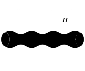
We consider an incompressible Newtonian ferrofluid cylinder of infinite length under a steady axisymmetric magnetic field of general shape. The ferrofluid response to the applied magnetic field is supposed to be linear, homogeneous and isotropic. Isothermal conditions are considered, and gravity is ignored. The surrounding fluid has no velocity, with negligible density and viscosity compared to the ferrofluid. An illustration of this basic state is shown in figure 3. The notations used in this figure will be progressively introduced into this section. The basic state, subjected to magnetic field  $\boldsymbol {H}_{\boldsymbol {0}}$, is characterised by the following conditions: zero velocity in each phase; an interface position at
  $r=R_0$ in a cylindrical coordinate system with
  $R_0$ the radius of the ferrofluid cylinder; a constant modified pressure
  $\varPi _{01}$ in the magnetic phase
  $(1)$; and a constant pressure
  $P_{02}$ in the non-magnetic phase
  $(2)$;
  $\varPi _{01}$ is related to
  $P_{02}$ by a surface tension contribution of magnitude
  $\sigma /R_0$, with
  $\sigma$ the surface tension, as well as by a constant magnetic contribution that will be specified below. We perturb this state by imposing a small-amplitude axisymmetric disturbance and we investigate whether the induced flow is linearly stable or unstable. The induced flow is characterised by its velocity
  $\boldsymbol {U}_{\boldsymbol {i}}$ in each phase
  $i$, its modified pressure
  $\varPi _i$, its magnetic field
  $\boldsymbol {H}_{\boldsymbol {i}}$ and the position of the interface at
  $r=r_s$. The vector fields are in the form
  $\boldsymbol {A}=(A_r,A_\theta ,A_z)$, where
  $A_r$,
  $A_\theta$ and
  $A_z$ are the radial, azimuthal and axial components of the vector, respectively. The different physical quantities are only dependent on coordinates
  $r$,
$r$,  $z$ and time
  $t$ due to the axisymmetry of the perturbation. The governing equations of this flow are described in the next subsections.

Figure 3. Representation of the basic state.
2.1. Bulk equations
The equations, valid for the ferrofluid, are first presented. The mass balance and momentum balance equations can be expressed as
 \begin{gather} \boldsymbol{\nabla} \boldsymbol{\cdot} \boldsymbol{U}_{\boldsymbol{1}}=0{,} \end{gather}
 \begin{gather}\rho_1\left(\frac{\partial \boldsymbol{U}_{\boldsymbol{1}}}{\partial t}+ \boldsymbol{U}_{\boldsymbol{1}} \boldsymbol{\cdot} \boldsymbol{\nabla} \boldsymbol{U}_{\boldsymbol{1}}\right)={-}\boldsymbol{\nabla} \varPi_1+\boldsymbol{\nabla} \boldsymbol{\cdot} \boldsymbol{\tau}_{\boldsymbol{\mathsf{1}}}, \end{gather}
with  $\rho _1$ the density,
  $\boldsymbol {\tau }_{\boldsymbol{\mathsf{1}}}=\eta _1(\boldsymbol {\nabla } \boldsymbol {U}_{\boldsymbol {1}}+\boldsymbol {\nabla } \boldsymbol {U}_{\boldsymbol {1}}^{\boldsymbol {t}})$ the viscous stress tensor,
  $\eta _1$ the dynamic viscosity and
  $\varPi _1$ defined by
  $\varPi _1=P_1+P_s$, where
  $P_1$ refers to thermodynamic pressure and
  $P_s=\mu _0 \int _0^H \upsilon (\partial M_1/\partial \upsilon )\,\textrm {d}H$ to the magnetostrictive pressure. In this last term,
  $\mu _0$ is the permeability of free space,
  $\upsilon$ the specific volume and
  $M_1$ the magnetisation.
A ferrofluid is not electrically conductive by nature, so Maxwell's equations are
 \begin{gather} \boldsymbol{\nabla} \boldsymbol{\cdot} \boldsymbol{B}_{\boldsymbol{1}}=0{,} \end{gather}
 \begin{gather}\boldsymbol{\nabla}\times\boldsymbol{H}_{\boldsymbol{1}}=\boldsymbol{0}{,} \end{gather}
with  $\boldsymbol {B}_{\boldsymbol {1}}$ the magnetic induction field which can be expressed as
 \begin{equation} \boldsymbol{B}_{\boldsymbol{1}}=\mu_0\left(\boldsymbol{H}_{\boldsymbol{1}}+\boldsymbol{M}_{\boldsymbol{1}} \right)=\mu_1 \boldsymbol{H}_{\boldsymbol{1}}{,} \end{equation}
with  $\mu _1$ the magnetic permeability of the ferrofluid, which is constant due to the linear, homogeneous and isotropic response of the medium. The equations valid for the surrounding fluid are (2.1) to (2.5) but with
  $\mu _2=\mu _0$ and negligible viscosity
  $\eta _2$ and density
  $\rho _2$.
2.2. Jump conditions across the interface
For jump conditions across the interface, the unit normal vector is introduced. It is defined at a point on the interface, pointing from the ferrofluid to the surrounding fluid, and is given by  $\boldsymbol {n}=\boldsymbol {\nabla }S/||\boldsymbol {\nabla }S||=1/\sqrt {1+(\partial r_s/\partial z)^2}\boldsymbol {e}_{\boldsymbol {r}}-(\partial r_s/\partial z)/\sqrt {1+(\partial r_s/\partial z)^2}\boldsymbol {e}_{\boldsymbol {z}}$, where
  $S=r-r_s$ is introduced to localise the position of the interface
  $S=0$. The first jump condition is obtained by writing the mass balance equation at the interface without mass exchange between two phases
 \begin{equation} \boldsymbol{U}_{\boldsymbol{1}} \boldsymbol{\cdot} \boldsymbol{n}={-} \frac{1}{||\boldsymbol{\nabla}S||}\frac{\partial S}{\partial t}\quad\text{at}\ r=r_s{.} \end{equation}
Regarding the jump conditions for momentum, there is continuity in the tangential component of stress acting on the interface
 \begin{equation} \left[\left(\boldsymbol{n} \boldsymbol{\cdot} \boldsymbol{\mathsf{T}}\right) \times\boldsymbol{n}\right]=\boldsymbol{0}\quad\text{at}\ r=r_s{,} \end{equation}
with the convention  $[A]=A_2-A_1$ and where
  $\boldsymbol{\mathsf{T}}$ is the stress tensor such that
  $\boldsymbol{\mathsf{T}}_{\boldsymbol{\mathsf{i}}}=-(P_i^*+( 1/2 )\mu _0 H_i^2)\boldsymbol{\mathsf{I}}+\boldsymbol {B}_{\boldsymbol {i}} \boldsymbol {H}_{\boldsymbol {i}}+\boldsymbol {\tau }_{\boldsymbol{\mathsf{i}}}$,
  $\boldsymbol{\mathsf{I}}$ the identity matrix,
  $P_i^*=\varPi _i+P_{mi}$ and
  $P_{mi}=\mu _0\int _0^H M_i\,\textrm {d}H$ the magnetic pressure. The jump of the normal component of the stress acting on the interface involves surface tension
 \begin{equation} \left[\left(\boldsymbol{n} \boldsymbol{\cdot} \boldsymbol{\mathsf{T}}\right)\boldsymbol{\cdot} \boldsymbol{n}\right]=\sigma\kappa\quad\text{at}\ r=r_s{,} \end{equation}
with  $\kappa =\boldsymbol {\nabla } \boldsymbol {\cdot } \boldsymbol {n}$ the total curvature.
The jump conditions for the magnetic field imply the continuity of the normal component of  $\boldsymbol {B}$ and the tangential component of
  $\boldsymbol {H}$ across the interface. Replacing
  $\boldsymbol {B}$ by expression (2.5), one finds
 \begin{gather} \mu_1 \boldsymbol{H}_{\boldsymbol{1}} \boldsymbol{\cdot} \boldsymbol{n}=\mu_0 \boldsymbol{H}_{\boldsymbol{2}} \boldsymbol{\cdot} \boldsymbol{n}\quad\text{at}\ r=r_s{,} \end{gather}
 \begin{gather}\boldsymbol{H}_{\boldsymbol{1}}\times\boldsymbol{n}=\boldsymbol{H}_{\boldsymbol{2}} \times\boldsymbol{n}\quad\text{at}\ r=r_s{.} \end{gather}
By using  $\boldsymbol {n} \boldsymbol {\cdot }\boldsymbol{\mathsf{I}}\times \boldsymbol {n}=\boldsymbol {0}$, (2.5), (2.9) and (2.10), (2.7) and (2.8) are reduced to
 \begin{gather} \left(\boldsymbol{n}\boldsymbol{\cdot}\boldsymbol{\tau}_{\boldsymbol{\mathsf{1}}}\right)\times \boldsymbol{n}=\boldsymbol{0}\quad\text{at}\ r=r_s{,} \end{gather}
 \begin{gather}P_1^*+P_n-\left(\boldsymbol{n}\boldsymbol{\cdot} \boldsymbol{\tau}_{\boldsymbol{\mathsf{1}}}\right)\boldsymbol{\cdot} \boldsymbol{n}=P_{2}+\sigma\boldsymbol{\nabla} \boldsymbol{\cdot} \boldsymbol{n}\quad\text{at}\ r=r_s{,} \end{gather}
with  $P_n=(1/2)\mu _0M_{1n}^2$ ; the
  $n$ index referring to the normal component.
2.3. Basic state and linearised dimensionless equations
The bulk equations for ferrofluid (2.1) and (2.2) and the jump conditions across the interface (2.6), (2.9)–(2.12) are made dimensionless by using the Rayleigh time  $\sqrt {\rho _1 R_0^3/\sigma }$,
  $R_0$,
  $\sigma /R_0$, an arbitrary magnetic field intensity
  $H_0$ and
  $\mu _0$ as characteristic time, length, pressure, magnetic field and magnetic permeability, respectively. The characteristic scales of the Rayleigh problem are chosen to enable the comparison of solutions with a magnetic field to those of the non-magnetic problem.
For the basic state, denoted by subscript  $0$ such that
  $\boldsymbol {H}_{{\boldsymbol {01}}}$ is the basic state of
  $\boldsymbol {H}_{\boldsymbol {1}}$ for example, the dimensionless equations become
 \begin{gather} \frac{\partial \varPi_{01}}{\partial r}=0{,} \end{gather}
 \begin{gather}\frac{\partial \varPi_{01}}{\partial z}=0{,} \end{gather}
 \begin{gather}\varPi_{01}+\tfrac{1}{2}N_{Bo,m}H_{01}^2+\tfrac{1}{2}\left(\mu_r-1\right)N_{Bo,m}H_{01r}^2=P_{02}+1\quad \text{at}\ r=1{,} \end{gather}
 \begin{gather}\mu_r H_{01r}=H_{02r}\quad\text{at}\ r=1{,} \end{gather}
 \begin{gather}H_{01\theta}=H_{02\theta}\quad\text{at}\ r=1{,} \end{gather}
 \begin{gather}H_{01z}=H_{02z}\quad\text{at}\ r=1{,} \end{gather}
with  $N_{Bo,m}=\mu _0 (\mu _r-1)H_0^2 R_0/\sigma$ the magnetic Bond number, and
  $\mu _r=\mu _1 /\mu _0$ the relative permeability;
  $N_{Bo,m}$ can be expressed as the product of two numbers
  $(\mu _r-1)$ and
  $\varGamma _m=\mu _0 H_0^2 R_0/\sigma$, with
  $\varGamma _m$ a magnetic parameter that does not depend on
  $\mu _r$. In (2.15),
  $M_{01}$ was replaced by
  $(\mu _r-1) H_{01}$ using relation (2.5) with
  $H_{01}$ corresponding to the norm of the vector
  $\boldsymbol {H_{01}}$. From this equation, it emerges that the magnetic field has an equivalent effect on pressure jump as occurs with surface tension.
The induced flow is decomposed around the basic state, as follows:  $U_i=u_i$,
  $\varPi _i=\varPi _{0i}+{\rm \pi} _i$,
  $H_i=H_{0i}+h_i$ and
  $r_s=1+\zeta$ with
  $u_i$,
  ${\rm \pi} _i$,
  $h_i$ the perturbed quantities in phase
  $i$ and
  $\zeta$ the surface perturbation. The dimensionless equations are linearised, and we thus obtain the equations for the perturbed quantities
 \begin{gather} \frac{1}{r}\frac{\partial r u_{1r}}{\partial r}+\frac{\partial u_{1z}}{\partial z}=0{,} \end{gather}
 \begin{gather}\frac{\partial u_{1r}}{\partial t}+\frac{\partial {\rm \pi}_1}{\partial r}-Oh\left( \frac{1}{r}\frac{\partial^2 r u_{1r}}{\partial r^2}-\frac{1}{r^2}\frac{\partial r u_{1r}}{\partial r}+\frac{\partial^2 u_{1r}}{\partial z^2}\right)=0{,} \end{gather}
 \begin{gather}\frac{\partial u_{1z}}{\partial t}+\frac{\partial {\rm \pi}_1}{\partial z}-Oh\left(\frac{1}{r}\frac{\partial r\dfrac{\partial u_{1z}}{\partial r}}{\partial r}+\frac{\partial^2 u_{1z}}{\partial z^2}\right)=0\text{,} \end{gather}
 \begin{gather}u_{1r}-\frac{\partial \zeta}{\partial t}=0\quad\text{at}\ r=1{,} \end{gather}
 \begin{gather}\frac{\partial u_{1r}}{\partial z}+\frac{\partial u_{1z}}{\partial r}=0\quad\text{at}\ r=1{,} \end{gather}
 \begin{gather} {\rm \pi}_1+N_{Bo,m}\left(H_{01}\frac{\partial H_{01}}{\partial r}\zeta+H_{01r}h_{1r}+H_{01z}h_{1z}+\left(\mu_r-1\right)\left(H_{01r}\frac{\partial H_{01r}}{\partial r}\zeta\right.\right.\nonumber\\ \hspace{3pc}\left.\left.+H_{01r}h_{1r}-H_{01r}H_{01z}\frac{\partial \zeta}{\partial z}\right)\right)-2Oh\frac{\partial u_{1r}}{\partial r}+\zeta+\frac{\partial^2 \zeta}{\partial z^2}=0\quad\text{at}\ r=1{,} \end{gather}
 \begin{gather} h_{2r}-\mu_r h_{1r}+\left(\mu_r-1\right)H_{01z}\frac{\partial \zeta}{\partial z}=0\quad\text{at}\ r=1{,} \end{gather}
 \begin{gather}h_{1\theta}-h_{2\theta}=0\quad\text{at}\ r=1\text{,} \end{gather}
 \begin{gather}h_{2z}-h_{1z}+\left(\mu_r-1\right)H_{01r}\frac{\partial \zeta}{\partial z}=0\quad\text{at}\ r=1{,} \end{gather}
with  $Oh=\eta _1/\sqrt {\rho _1 \sigma R_0}$ the Ohnesorge number. The last three equations were simplified using (2.16)–(2.18).
In these equations, the magnetic field interferes with the hydrodynamic problem in the pressure term and the pressure jump across the interface.
The system of equations is linear with respect to  $t$ and
  $z$, and nonlinear with respect to
  $r$. Hence, we seek solutions in the form
  $A(r)\exp ({\textrm {i}kz+\alpha t})$, where
  $A(r)$ is an unknown function of
  $r$. Since this study explores temporal stability, we take
  $k$ to be real, and
  $\alpha =\alpha _r + \textrm {i} \alpha _i$ to be complex, such that
  $k$,
$k$,  $\alpha _r$ and
  $\alpha _i$ are respectively the wavenumber, growth rate and oscillation frequency of the perturbation.
3. Solution
In this section, we first determine the admissible magnetic field shapes. Then, a dispersion relation and a cutoff wavenumber equation adapted to each shape are derived.
3.1. Admissible magnetic fields
Based on the assumptions made in this paper, the magnetic field cannot have an arbitrary shape. It is supposed to be axisymmetric and must satisfy Maxwell equations (2.3) and (2.4), which were developed after considering a steady magnetic field and fluid that is not electrically conductive. Thus, the admissible magnetic fields must satisfy
 \begin{gather} \frac{\partial H_{01\theta}}{\partial z}=0{,} \end{gather}
 \begin{gather}\frac{\partial H_{01r}}{\partial z}-\frac{\partial H_{01z}}{\partial r}=0{,} \end{gather}
 \begin{gather}H_{01\theta}+r\frac{\partial H_{01\theta}}{\partial r}=0{,} \end{gather}
 \begin{gather}\frac{\partial H_{01r}}{\partial r}+\frac{H_{01r}}{r}+\frac{\partial H_{01z}}{\partial z}=0{.} \end{gather}
From (3.1) and (3.3), the azimuthal component must be in the form  $H_{01\theta }=B/r$, with
  $B$ a constant. From the basic state, it is visible that the different components of
  $\boldsymbol {H}_{\boldsymbol {01}}$ must be independent of
  $z$. Equations (2.13) and (2.14) show that
  $\varPi _{01}$ is constant. Moreover, it can be shown that
  $P_{02}$ follows the same equations and is also a constant, hence the
  $z$ independence of
  $\boldsymbol {H_{01}}$ seen in relation (2.15). From relations (3.2) and (3.4), it follows that
  $H_{01z}$ is a constant and that component
  $H_{01r}$ must be in the form
  $A/r$, with
  $A$ a constant. Therefore, only the shape
  $\boldsymbol {H}_{\boldsymbol {01}}=(A/r,B/r,C)$ with
  $C$ a constant is admissible.
Two cases can be distinguished: axial magnetic fields ( $A=0,B=0,C\neq 0$) and non-axial magnetic fields (
 $A\neq 0$ or
  $B\neq 0$). For this last case, a solid cylindrical structure (which can be a hollow or solid wire) is necessary at
  $r=0$ to overcome the singularity. These two cases have different boundary conditions and are thus solved separately in the following. The methodology used to solve the equations will be detailed for the axial case. For the other case, only what differs from the axial case will be specified.
3.2. Axial magnetic fields
3.2.1. Dispersion relation
To solve the linearised equations and obtain the dispersion relation, the methodology used by Renoult et al. (Reference Renoult, Brenn, Plohl and Mutabazi2018) for the case of a non-magnetic liquid jet is followed. Because the velocity is divergence free, it can be expressed with a Stokes streamfunction  $\psi$ in the form
  $u_{1r}=-(1/r)(\partial \psi _1/\partial z)$ and
  $u_{1z}=(1/r)(\partial \psi _1/\partial r)$. Furthermore, the magnetic field
  $h$ is curl free, and thus there exists a magnetic perturbation potential
  $\phi$ for each phase such that
  $\boldsymbol {h}_{\boldsymbol {1}}=-\boldsymbol {\nabla }\phi _1$ and
  $\boldsymbol {h}_{\boldsymbol {2}}=-\boldsymbol {\nabla }\phi _2$. The equations to be solved can be written in the following form:
 \begin{gather} \frac{\partial {\rm \pi}_1}{\partial r}=\frac{1}{r}\frac{\partial^2 \psi_1}{\partial z\partial t}+\frac{Oh}{r}\left(\frac{1}{r}\frac{\partial^2 \psi_1}{\partial r\partial z}-\frac{\partial^3 \psi_1}{\partial r^2\partial z}-\frac{\partial^3 \psi_1}{\partial z^3}\right){,} \end{gather}
 \begin{gather}\frac{\partial {\rm \pi}_1}{\partial z}={-}\frac{1}{r}\frac{\partial^2 \psi_1}{\partial r\partial t}+\frac{Oh}{r}\left(\frac{\partial^3 \psi_1}{\partial r^3}-\frac{1}{r}\frac{\partial^2 \psi_1}{\partial r^2}+\frac{1}{r^2}\frac{\partial \psi_1}{\partial r}+\frac{\partial^3 \psi_1}{\partial z^2\partial r}\right){,} \end{gather}
 \begin{gather}-\frac{\partial \psi_1}{\partial z}=\frac{\partial \zeta}{\partial t}\quad \text{at}\ r=1{,} \end{gather}
 \begin{gather}\frac{\partial^2 \psi_1}{\partial r^2}-\frac{\partial \psi_1}{\partial r}-\frac{\partial^2 \psi_1}{\partial z^2}=0\quad\text{at}\ r=1{,} \end{gather}
 \begin{gather}{\rm \pi}_1=N_{Bo,m} \frac{\partial \phi_1}{\partial z}+2Oh\left(\frac{\partial \psi_1}{\partial z}-\frac{\partial^2 \psi_1}{\partial r\partial z}\right)-\zeta-\frac{\partial^2 \zeta}{\partial z^2}\quad\text{at}\ r=1{,} \end{gather}
 \begin{gather}\mu_r\frac{\partial \phi_1}{\partial r}-\frac{\partial \phi_2}{\partial r}+\left(\mu_r-1\right)\frac{\partial \zeta}{\partial z}=0\quad\text{at}\ r=1{,} \end{gather}
 \begin{gather}\frac{\partial \phi_1}{\partial z}-\frac{\partial \phi_2}{\partial z}=0\quad\text{at}\ r=1{.} \end{gather}
Differentiating (3.5) with respect to  $z$ and (3.6) with respect to
  $r$, it can be shown that
 \begin{equation} \left(\frac{\partial^2}{\partial r^2}-\frac{1}{r}\frac{\partial}{\partial r}+\frac{\partial^2}{\partial z^2}-\frac{1}{Oh}\frac{\partial}{\partial t}\right)\left(\frac{\partial^2}{\partial r^2}-\frac{1}{r}\frac{\partial}{\partial r}+\frac{\partial^2}{\partial z^2}\right)\psi_1=0{.} \end{equation}
The solution  $\psi _1$ is the sum of two contributions and has the form
 \begin{equation} \psi_1=r(\hat{A}I_1(kr)+\check{A}I_1(lr)+\hat{B}K_1(kr)+\check{B}K_1(lr)) \exp({\textrm{i}kz+\alpha t}){,} \end{equation}
with  $I_1$ and
  $K_1$ the modified Bessel functions of the first and second kinds, and
  $l^2=k^2+(\alpha /Oh)$ a modified wavenumber. The streamfunction must be finite at
  $r=0$ so
  $\hat {B}=0$ and
  $\check {B}=0$. Furthermore, by using (3.8), we find that
 \begin{equation} \psi_1=r\hat{A}\left[I_1(kr)-\frac{2k^2}{k^2+l^2}\frac{I_1(k)}{I_1(l)}I_1(lr)\right]\exp({\textrm{i}kz+\alpha t}){.} \end{equation}
Integrating (3.7) in time, it follows that
 \begin{equation} \zeta=\textrm{i}\frac{k}{\alpha}\hat{A}I_1(k)\left[\frac{k^2-l^2}{k^2+l^2}\right]\exp({\textrm{i}kz+\alpha t}){.} \end{equation}
The constant of integration in relation (3.15) is zero by definition of  $\zeta$. Then,
  ${\rm \pi} _1$ is obtained by integrating (3.6) with respect to
  $z$ and using (3.5) to find the constant of integration
 \begin{equation} {\rm \pi}_1=\textrm{i}\alpha\hat{A}I_0(kr)\exp({\textrm{i}kz+\alpha t}){.}\end{equation}
The next step is to determine  $\phi$ in each phase. With (2.3) and (2.5), we see that
  $\Delta \phi =0$ in each phase leading to
 \begin{gather} \phi_1=\left(a_1 I_0(kr)+b_1 K_0(kr)\right)\exp({\textrm{i}kz+\alpha t}){,} \end{gather}
 \begin{gather}\phi_2=\left(a_2 I_0(kr)+b_2 K_0(kr)\right)\exp({\textrm{i}kz+\alpha t}){.} \end{gather}
The potential should be finite at  $r=0$ and there is no perturbation when
  $r$ tends to infinity, so
  $b_1=0$ and
  $a_2=0$;
  $a_1$ and
  $b_2$ are determined using relations (3.10) and (3.11), thus giving
 \begin{equation} \phi_1=\left[\frac{k}{\alpha}\hat{A}I_1(k)\left[\frac{k^2-l^2}{k^2+l^2}\right]\frac{\left(\mu_r-1\right)K_0(k)}{\mu_r I_1(k)K_0(k)+I_0(k)K_1(k)}\right]I_0(kr)\exp({\textrm{i}kz+\alpha t}){.} \end{equation}
Finally, the dispersion relation is obtained with the jump condition (3.9)
 \begin{align} &\alpha^2+2\alpha k^2Oh\left[1-\frac{I_1(k)}{I_0(k)}\left(\frac{1}{k}+\frac{2kl}{l^2+k^2}\left(\frac{I_0(l)}{I_1(l)} -\frac{1}{l}\right)\right)\right]\nonumber\\ &\quad -k(1-k^2+P_{mag})\frac{I_1(k)}{I_0(k)}\frac{l^2-k^2}{l^2+k^2}=0\text{,} \end{align}
with
 \begin{equation} P_{mag}={-}N_{Bo,m}\left(\mu_r-1\right) k\frac{I_0(k)K_0(k)}{\mu_r I_1(k)K_0(k)+I_0(k)K_1(k)}{,} \end{equation}
the magnetic field contribution to the dispersion relation. This relation is a transcendental equation due to the term  $I_0(l)/I_1(l)$, which depends on
  $\alpha$. It tends towards the relation of the Newtonian case in the absence of a magnetic field, so when
  $N_{Bo,m}=0$, as reported in García & González (Reference García and González2008) with a different representation (note that the two representations are equivalent Brenn Reference Brenn2017). Because the magnetic contribution
  $P_{mag}$ does not depend on
  $\alpha$, the same number of solutions as the non-magnetic case is expected. Therefore, the dispersion relation (3.20) has a trivial solution
  $\alpha =0$, two capillary solutions, and an infinite number of hydrodynamic solutions using the same terminology as García & González (Reference García and González2008). The trivial and hydrodynamic solutions appear when viscosity is taken into account. The hydrodynamic solutions come from the fact that
  $l$ is a complex number depending on
  $\alpha$ and that
  $I_1(l)$ has an infinite number of roots. By taking the limit
  $Oh\rightarrow 0$, the dispersion relation first obtained by Taktarov (Reference Taktarov1975) is found (with a typographical error in the dispersion relation where a modified Bessel function
  $I_1$ is replaced by
  $I_0$).
3.2.2. Cutoff wavenumber
The cutoff wavenumber  $k_c$ is the wavenumber for which
  $\alpha _r$ changes from positive to negative (or from negative to positive) values, corresponding to the transition from the unstable to stable (or from the stable to unstable) regime. To determine it, the dispersion relation is written to eliminate the trivial solution. Simplifying by
  $\alpha$
 \begin{align} &\alpha+2k^2Oh\left[1-\frac{I_1(k)}{I_0(k)}\left(\frac{1}{k}+\frac{2kl}{l^2+k^2}\left(\frac{I_0(l)}{I_1(l)}- \frac{1}{l}\right)\right)\right]\nonumber\\ &\quad -k(1-k^2+P_{mag})\frac{I_1(k)}{I_0(k)}\frac{1}{Oh\left(l^2+k^2\right)}=0{.} \end{align}
Then,  $k_c$ corresponds to the wavenumber for which
  $\alpha =0$. By taking
  $\alpha =0$, we have
  $l^2=k_c^2$ and relation (3.22) becomes
 \begin{equation} -k_c(1-k_c^2+P_{mag})\frac{I_1(k_c)}{I_0(k_c)}\frac{1}{2Oh k_c^2}=0\text{.} \end{equation}
Only  $(1-k_c^2+P_{mag})$ can be cancelled, so relation (3.23) is verified when
 \begin{equation} k_c^2+k_c\frac{I_0(k_c)K_0(k_c)}{\mu_r I_1(k_c)K_0(k_c)+I_0(k_c)K_1(k_c)}\left(\mu_r-1\right)N_{Bo,m}-1=0{.} \end{equation}
From this equation, it is shown that  $k_c$ is independent of
  $Oh$.
$Oh$.
3.2.3. Presence of a solenoid
Experimentally, one way to create an axial magnetic field is to use a solenoid (figure 4). It consists in a solid cylindrical structure enclosing the ferrofluid cylinder in the surrounding fluid. Therefore, the presence of a solenoid with a radius  $R_s$ leads to a supplementary boundary condition for the magnetic perturbation potential
 \begin{equation} \phi_2=0\quad\text{at}\ r=\delta_s{,} \end{equation}
with  $\delta _s=R_s/R_0$ the dimensionless solenoid radius. Thus, constant
  $a_2$ in relation (3.18) is no longer zero but is expressed as a function of
  $b_2$, leading to a new expression for
  $\phi _1$. Only the expression of
  $\phi _1$ (and obviously
  $\phi _2$) is modified by the presence of the solenoid. Hence, the dispersion relation has the same form as relation (3.20) but with a different expression for
  $P_{mag}$ given by
 \begin{equation} P_{mag}={-}N_{Bo,m}\left(\mu_r - 1\right) k\frac{I_0(k)A_s}{\mu_r I_1(k)A_s+I_0(k)B_s}{,} \end{equation}
with  $A_s=I_0(k\delta _s)K_0(k)-I_0(k)K_0(k\delta _s)$ and
  $B_s=I_1(k)K_0(k\delta _s)+I_0(k\delta _s)K_1(k)$.

Figure 4. Representation of a ferrofluid cylinder enclosed by a solenoid.
The cutoff wavenumber for an axial magnetic field with a solenoid can also be predicted by solving the following equation:
 \begin{equation} k_c^2+k_c\frac{I_0(k_c)A_s}{\mu_r I_1(k_c)A_s+I_0(k_c)B_s}\left(\mu_r-1\right)N_{Bo,m}-1=0{,} \end{equation}
derived from the cancellation of  $(1-k_c^2+P_{mag})$. This equation tends to (3.24) for a high value of
  $\delta _s$.
3.3. Non-axial magnetic fields
3.3.1. Dispersion relation
For this kind of magnetic field, the constants  $A$,
$A$,  $B$ and
  $C$ in
  $\boldsymbol {H}_{\boldsymbol {01}}=(A/r,B/r,C)$ are all susceptible to having a non-zero value. Therefore, (3.9)–(3.11) have the following more general form:
 \begin{gather} \hspace{-2.5pc}{\rm \pi}_1={-}N_{Bo,m}\left(-\left(A^2+B^2\right)\zeta-A\frac{\partial \phi_1}{\partial r}-C\frac{\partial \phi_1}{\partial z}+\left(\mu_r-1\right)\left(\vphantom{\frac{\partial \phi_1}{\partial r}}-A^2\zeta\right.\right.\nonumber\\ \hspace{3pc}\left.\left.-A\frac{\partial \phi_1}{\partial r}-AC\frac{\partial \zeta}{\partial z}\right)\right)+2Oh\left(\frac{\partial \psi_1}{\partial z}-\frac{\partial^2 \psi_1}{\partial r\partial z}\right)-\zeta-\frac{\partial^2 \zeta}{\partial z^2}\quad\text{at}\ r=1{,} \end{gather}
 \begin{gather} \mu_r\frac{\partial \phi_1}{\partial r}-\frac{\partial \phi_2}{\partial r}+\left(\mu_r-1\right)C\frac{\partial \zeta}{\partial z}=0\quad\text{at}\ r=1{,} \end{gather}
 \begin{gather} \frac{\partial \phi_1}{\partial z}-\frac{\partial \phi_2}{\partial z}+\left(\mu_r-1\right)A\frac{\partial \zeta}{\partial z}=0\quad\text{at}\ r=1{.} \end{gather}
 Then, due to the presence of a wire of radius  $R_w$ (figure 5), the dispersion relation no longer has the same form. Indeed, the singularity at
  $r=0$ is removed, and constants
  $\hat {B}$ and
  $\check {B}$ are no longer equal to zero in relation (3.13). Two further boundary conditions are needed: no penetration and no slip at the wire surface, which can be written into the following form
 \begin{equation} {-}\frac{1}{r}\frac{\partial \psi_1}{\partial z}=0\quad\text{and}\quad \frac{1}{r}\frac{\partial \psi_1}{\partial r}=0\quad\text{at}\ r=\delta_w{,} \end{equation}
with  $\delta _w=R_w/R_0$ the dimensionless wire radius. Using relation (3.31a,b) and the same methodology as in § 3.2.1, new expressions are found for
  $\psi _1$,
  $\zeta$ and
  ${\rm \pi} _1$. The presence of the wire also leads to an additional boundary condition for the magnetic perturbation potential
 \begin{equation} \phi_1=0\quad\text{at}\ r=\delta_w{.} \end{equation}
Thus, constant  $b_1$ in relation (3.18) is no longer zero but expressed as a function of
  $a_1$, thus modifying the expression of
  $\phi _1$. Finally, the new dispersion relation is obtained through relation (3.28)
 \begin{align} &\alpha^2+2\alpha k^2Oh\left[1-\frac{1}{k}\left(I_1(k)-\textrm{d}I_1(l)-\left(\frac{cd-a}{b}\right)K_1(k) +\left(\frac{cd-a}{b}\right)\frac{K_1(k\delta_w)}{K_1(l\delta_w)}K_1(l)\right.\right.\nonumber\\ &\quad +d\frac{I_1(l\delta_w)}{K_1(l\delta_w)}K_1(l)-\frac{I_1(k\delta_w)}{K_1(l\delta_w)}K_1(l)+ \textrm{d}l I_0(l) +\left(\frac{cd-a}{b}\right)\frac{K_1(k\delta_w)}{K_1(l\delta_w)}K_0(l)l \nonumber\\ &\quad \left.\left.+\,d\frac{I_1(l\delta_w)}{K_1(l\delta_w)}K_0(l)l-\frac{I_1(k\delta_w)}{K_1(l\delta_w)}K_0(l)l\right) \left(\frac{1}{I_0(k)+\left(\dfrac{cd-a}{b}\right)K_0(k)}\right)\right] \nonumber\\ &\quad -k(1-k^2+P_{mag}) \left(I_1(k)-\textrm{d}I_1(l) -\left(\frac{cd-a}{b}\right)K_1(k)+\left(\frac{cd-a}{b}\right)\frac{K_1(k\delta_w)}{K_1(l\delta_w)}K_1(l)\right.\nonumber\\ &\quad \left.+\,d\frac{I_1(l\delta_w)}{K_1(l\delta_w)}K_1(l)-\frac{I_1(k\delta_w)}{K_1(l\delta_w)}K_1(l)\right) \left(\frac{1}{I_0(k)+\left(\dfrac{cd-a}{b}\right)K_0(k)}\right)=0{,} \end{align}
with constants  $a$,
$a$,  $b$,
$b$,  $c$,
$c$,  $d$ and the magnetic field contribution
  $P_{mag}$ defined as
 \begin{gather} a=k I_0(k\delta_w)K_1(l\delta_w)+l I_1(k\delta_w)K_0(l\delta_w){,} \end{gather}
 \begin{gather}b=k K_0(k\delta_w)K_1(l\delta_w)-l K_1(k\delta_w)K_0(l\delta_w){,} \end{gather}
 \begin{gather}c=l I_0(l\delta_w)K_1(l\delta_w)+l I_1(l\delta_w)K_0(l\delta_w){,} \end{gather}
 \begin{gather}d=\frac{2k^2 K_1(l\delta_w)\left(bI_1(k)+aK_1(k)\right)-\left(k^2+l^2\right)K_1(l)\left(bI_1(k\delta_w)+aK_1(k\delta_w)\right)}{2k^2 K_1(l\delta_w)cK_1(k)-\left(k^2+l^2\right)\left(K_1(l)\left(bI_1(l\delta_w)+cK_1(k\delta_w)\right)-bI_1(l)K_1(l\delta_w)\right)}{,} \end{gather}
 \begin{gather}P_{mag}={-}N_{Bo,m}\left[\mu_r A^2+B^2-\frac{\left(\mu_r-1\right)k\left(\mu_r A^2 A_w K_1(k)-C^2 B_w K_0(k)\right)}{\mu_r A_w K_0(k)+ B_w K_1(k)}\right]{,} \end{gather}
where  $A_w=I_1(k)K_0(k\delta _w)+I_0(k\delta _w)K_1(k)$ and
  $B_w=I_0(k)K_0(k\delta _w)-I_0(k\delta _w)K_0(k)$. The dispersion relation is coherent with that obtained by Arkhipenko et al. (Reference Arkhipenko, Barkov, Bashtovoi and Krakov1981) in the inviscid limit without surrounding fluid (with a typographical error in the dispersion relation where the numerator and denominator were inverted, as well as the sign of one of the terms).

Figure 5. Representation of a ferrofluid cylinder with a wire.
3.3.2. Cutoff wavenumber
From the dispersion relation (3.33), it is possible to obtain the equation for the cutoff wavenumber. It is not obvious a priori that  $\alpha =0$ is a solution of relation (3.33) but it can be proved by using Taylor series. It can also be shown that the cutoff wavenumber equation is still obtained by the cancellation of
  $(1-k_c^2+P_{mag})$, leading to
 \begin{align} k_c^2+k_c\frac{C^2 B_w K_0(k_c)-\mu_r A^2 A_w K_1(k_c)}{\mu_r A_w K_0(k_c)+B_w K_1(k_c)}\left(\mu_r-1\right)N_{Bo,m}-(1-N_{Bo,m}(\mu_r A^2+B^2))=0{.} \end{align}
If  $k_c=0$ is the solution of this equation, this means that the ferrofluid cylinder is stable for all wavenumbers (for cases where only one positive cutoff wavenumber exists). This total stability is obtained when the following condition is verified:
 \begin{equation} N_{Bo,m}(\mu_r A^2+B^2)-1=0{.} \end{equation}
3.4. Applicability to jet description
In this paper, we perform a temporal stability analysis of a doubly infinite liquid cylinder. We examine the applicability of this analysis to a jet description. In fact, as explained in the introduction, a spatial stability analysis is more appropriate. In this case, the solutions are searched under the form  $A_s (r)\exp ({\textrm {i}(k_s z-\alpha _s t)})$, but this time,
  $k_s$ is a complex number and
  $\alpha _s$ a real number. Consequently, the perturbation oscillates over time and grows with distance
  $z$ when
  $k_s$ has a negative imaginary part. Using the same methodology as in Keller et al. (Reference Keller, Rubinow and Tu1973), the following dimensionless parameters are introduced:
  $x=k_s R_0$,
  $\omega =\alpha _s R_0/V_{jet}$ and
  $\beta =V_{jet}\sqrt {\rho R_0/\sigma }$ with
  $\beta$ the dimensionless jet velocity. Dimensionless solutions can be expressed in a stationary coordinate system by replacing
  $z$ by
  $z+\beta t$, giving
  $A(r)\exp ({\textrm {i}(xz-(\omega -x)\beta t)})$. Comparing this solution to that obtained from temporal analysis (i.e.
  $A(r)\exp ({\textrm {i}kz+\alpha t})$), the dispersion relation of the spatial analysis is obtained by replacing
  $k$ by
  $x$ and
  $\alpha$ by
  $-\textrm {i}\beta (\omega -x)$ in the temporal analysis. Keller et al. (Reference Keller, Rubinow and Tu1973) show a correspondence between the unstable spatial and temporal solution for
  $\beta \gg 1$, so when the dimensionless jet velocity is relatively high.
In the following section, different cases corresponding to different magnetic field shapes will be examined. For the axial case without solid core, we search the values of  $\beta$ for which the unstable solution for the temporal analysis is also a solution for the spatial analysis. Contrary to the work of Guerrero et al. (Reference Guerrero, González and García2012), where all spatial modes are studied, we restrict here the
  $\beta$ search to the most unstable mode. For the temporal analysis, it is characterised by
  $\textrm {Re}(\alpha )=\alpha _{r}^{*}$,
  $\textrm {Im}(\alpha )=0$ and
  $k=k^{*}$. Comparing once again the form of the solutions in temporal and spatial analyses, a link can be made between
  $k$ and
  $\textrm {Re}(x)$, between
  $\textrm {Re}(\alpha )$ and
  $-\beta \,\textrm {Im}(x)$, and between
  $\textrm {Im}(\alpha )$ and
  $\beta (\textrm {Re}(x)-\omega )$. Therefore, in the dispersion relation of the spatial analysis,
  $\textrm {Re}(x)=k^{*}$,
  $\textrm {Im}(x)=-\alpha _{r}^{*}/\beta$ and
  $\omega =\textrm {Re}(x)$. This dispersion relation becomes a function that is only dependent on
  $\beta$,
  $f(\beta )=0$. We thus search for values of
  $\beta$ that give
  $|\kern0.06em f(\beta )|<\epsilon$, where
  $\epsilon$ is the set convergence criterion and does not represent the difference between the dominant modes obtained with spatial and temporal analyses. For example, applying this method to the inviscid non-magnetic case and setting
  $\epsilon =10^{-4}$ leads to a difference of 0.026 %.
4. Applications
This section considers magnetic fields investigated in the literature or presenting a special interest. These magnetic fields can be written in the general form  $\boldsymbol {H}_{\boldsymbol {01}}=(A/r,B/r,C)$ with the appropriate choice of constants
  $A$,
$A$,  $B$ and
  $C$. Only this form of magnetic field shape was previously shown to be admissible. The transcendental dispersion relations (3.20) and (3.33) are solved using the method of Luck, Zdaniuk & Cho (Reference Luck, Zdaniuk and Cho2015) and the transcendental cutoff wavenumber equations using a zero-search procedure. The effect of magnetic field intensity and the type of ferrofluid are characterised by varying
  $\varGamma _m$ and
  $\mu _r$. Indeed, we chose to vary
  $\varGamma _m$ instead of
  $N_{Bo,m}$ in order to have a parameter independent of
  $\mu _r$. Finally, the experimental applicability of the theory is studied. Previous experiments are reported in table 1 with the typical values of magnetic fields.
Table 1. Experimental conditions of previous experiments on ferrofluid jets and cylinders. Unknown data are represented by the symbol  $\bullet$. Data in brackets are used for estimations.

Table 2. Ferrofluid properties under standard laboratory conditions. Unknown data are represented by the symbol  $\bullet$.

4.1. Axial magnetic field
The first studied case is a constant axial magnetic field with the form  $\boldsymbol {H}_{\boldsymbol {01}}=(0,0,1)$, which corresponds to the form
  $\boldsymbol {H}_{\boldsymbol {01}}=(A/r,B/r,C)$ with
  $\lbrace A=0 ; B=0\ ; C=1\rbrace$. The dispersion relation associated with this case is given by (3.20).
The growth rate and pulsation of the dispersion relation solutions are shown in figure 6 as functions of the wavenumber for different  $\varGamma _m$. Recall that
  $N_{Bo,m}$ is defined by
  $N_{Bo,m}=(\mu _r -1)\varGamma _m$.
  $Oh$ and
  $\mu _r$ are set to
  $0.55$ and
  $2$, respectively. With this value of
  $\mu _r$,
  $N_{Bo,m}=\varGamma _m$. The solutions obtained by García & González (Reference García and González2008) are determined for
  $\varGamma _m=0$, namely a trivial solution
  $\alpha =0$, two capillary solutions and an infinite number of hydrodynamic solutions. Only two hydrodynamic solutions are visible owing to the chosen window for the values of
  $\alpha$. Here,
  $\varGamma _m$ depends on
  $\sigma$,
  $R_0$ and
  $H_0$;
  $H_0$ is not necessarily defined as the applied magnetic field intensity even if it is the case here. If the same ferrofluid cylinder is considered (same
  $\sigma$ and
  $R_0$), a modification of
  $\varGamma _m$ thus implies a modification of the magnetic field intensity
  $H_0$. Thus, varying
  $\varGamma _m$ shows the effect of
  $H_0$ on the stability of the liquid cylinder. In this figure, different behaviours can be distinguished: an unstable regime without oscillation characterised by
  $\alpha _r>0$ and
  $\alpha _i=0$ delimited by
  $k_c$, a stable regime without oscillation characterised by
  $\alpha _r<0$ and
  $\alpha _i=0$ and a stable oscillating regime characterised by
  $\alpha _r<0$ and
  $\alpha _i\ne 0$ delimited by two wavenumbers
  $k_1$ and
  $k_2$. Increasing
  $\varGamma _m$ induces an extension of the stable oscillating regime with a higher frequency of oscillation. It also reduces
  $k_c$ and
  $\alpha _r$ in the unstable regime, hence increasing the extension of the stable regime.

Figure 6. Solutions of the dispersion relation in an axial magnetic field for  $Oh=0.55$,
  $\mu _r=2$ and different
  $\varGamma _m$; (a,b)
  $\alpha _r$ as a function of
  $k$, (c,d)
  $\alpha _i$ as a function of
  $k$. Panels (b,d) are blow-ups of (a,c); ——
  $\varGamma _m=0$; — - –
  $\varGamma _m=1$; — —
  $\varGamma _m=5$; - - - - - - - -
  $\varGamma _m=10$. Black lines correspond to the capillary solutions and grey lines to the hydrodynamic solutions. Vertical dotted lines represent the values of
  $k_c$,
  $k_1$ and
  $k_2$ for
  $\varGamma _m=0$.
The behaviour of  $k_c$ can be predicted with the help of (3.24). The solution of this equation as a function of
  $\varGamma _m$ is represented in figure 7. The stabilisation of the cylinder when
  $\varGamma _m$ increases is confirmed, and the cutoff wavenumbers visible in figure 6(b) are identified. High values of
  $\varGamma _m$ (or
  $N_{Bo,m}$), like those plotted here, can be encountered experimentally as shown in table 1. However, the cylinder is never totally stable for an axial magnetic field. The zero value for
  $k_c$ is an asymptotic value approached for
  $\varGamma _m$ tending to infinity.

Figure 7. Value of  $k_c$ as a function of
  $\varGamma _m$ for
  $\mu _r=2$. The inset is a blow-up in the vicinity of low
  $\varGamma _m$.
To examine the influence of the magnetic fluid on the solutions of the dispersion relation,  $\mu _r$ is varied for a constant
  $\varGamma _m=1$, and
  $Oh$ is kept at
  $0.55$ (figure 8). The same behaviour, as in varying
  $\varGamma _m$, is observed: reduction in
  $k_c$ and
  $\alpha _r$, and extension of the stable oscillating regime with a higher frequency of oscillation. This shows that, in this case, having ferrofluid with a higher relative magnetic permeability has the same effect as increasing the magnetic field intensity.

Figure 8. Solutions of the dispersion relation in an axial magnetic field for  $Oh=0.55$,
  $\varGamma _m=1$ and different
  $\mu _r$; (a,b)
  $\alpha _r$ as a function of
  $k$, (c,d)
  $\alpha _i$ as a function of
  $k$. Panels (b,d) are blow-ups of (a,c); ——
  $\mu _r=1$; — —
  $\mu _r=3$; - - - - - - - -
  $\mu _r=5$. Black lines correspond to the capillary solutions and grey lines to the hydrodynamic solutions.
The influence of  $Oh$ on the dispersion relation is described in the literature for the non-magnetic cases (García & González Reference García and González2008): reduction in growth rate and wavenumber for the most unstable mode when
  $Oh$ increases, independence of
  $Oh$ on
  $k_c$ and dependence of
  $Oh$ on
  $k_1$ and
  $k_2$ with a disappearance of the stable oscillating regime for a sufficiently high value of
  $Oh$. The non-modification of
  $k_c$ with respect to
  $Oh$ is visible in figure 9 (dotted lines) for different values of
  $\varGamma _m$. However, the evolution of
  $k_1$ and
  $k_2$ as a function of
  $Oh$ (solid lines) is modified with the magnetic field. As
  $\varGamma _m$ increases,
  $k_1$ becomes increasingly independent of
  $Oh$, and for large values of
  $Oh$,
$Oh$,  $k_2$ varies more slowly. For lower values of
  $Oh$, the
  $k_2$ values for the different
  $\varGamma _m$ seem to converge, as
  $k_1$ becomes closer to
  $k_c$. Moreover, the disappearance of the stable oscillating regime appears for higher values of
  $Oh$ as
  $\varGamma _m$ increases.

Figure 9. Delimitation of the different stability regimes for any value of  $k$ and
  $Oh$,
$Oh$,  $\mu _r=2$ and different
  $\varGamma _m$. From the darkest to the lightest,
  $\varGamma _m=0$,
  $\varGamma _m=1$,
  $\varGamma _m=3$,
  $\varGamma _m=5$ and
  $\varGamma _m=10$. Vertical dotted lines represent the corresponding value of
  $k_c$, and solid lines separate the regimes with and without oscillations delimited by
  $k_1$ and
  $k_2$ values.
Experimentally, an axial magnetic field can be created using a solenoid of radius  $R_s$ and length
  $L_s$. We first assume that the length is infinite. Thus, the magnetic field created by the solenoid is
 \begin{equation} \boldsymbol{H}=\boldsymbol{e}_{\boldsymbol{z}}{,} \end{equation}
choosing  $H_0=In$ (characteristic magnetic field used to make
  $\boldsymbol {H}$ dimensionless) with
  $I$ the current intensity in the solenoid and
  $n$ the number of turns by unit of length. This expression is a classical result, which is found in books on electromagnetism: e.g. Smythe (Reference Smythe1950), Jackson (Reference Jackson1962) and Pérez et al. (Reference Pérez, Carles, Fleckinger and Lagoute2009). The solenoid is in this case considered as a stack of
  $N$ loops. In reality, the solenoid is a winding of wire; nevertheless, expression (4.1) is valid to within
  $1\,\%$ if the pitch of the winding does not exceed
  $1.35\ R_s$, which is often the case. The solutions for relation (3.20), with expression (3.26) for
  $P_{mag}$, are plotted in figure 10 for
  $Oh=0.55$,
  $\mu _r=2$,
  $\varGamma _m=1$ and different values of
  $\delta _s$. The curves are very close to each other for different values of
  $\delta _s$, and the largest offset between them is for
  $k$ around the cutoff wavenumber. This can be explained by the fact that in the dispersion relation,
  $\delta _s$ only appears in
  $P_{mag}$, which is related to the cutoff wavenumber. A blow-up around
  $k_c$ is shown in the inset, where a convergence to the solution without a solenoid is observed by increasing the value of
  $\delta _s$. The curve for
  $\delta _s=5$ seems to coincide with the curve which corresponds to the case without a solenoid. Consequently, for this case (
 $Oh=0.55$,
  $\mu _r=2$ and
  $\varGamma _m=1$), we can neglect the effect of the solenoid if its radius is more than five times than that of the initial cylinder.

Figure 10. Solutions of the dispersion relation in an axial magnetic field created by a solenoid for  $Oh=0.55$,
  $\varGamma _m=1$,
  $\mu _r=2$ and different
  $\delta _s$; (a,b)
  $\alpha _r$ as a function of
  $k$, (c,d)
  $\alpha _i$ as a function of
  $k$. Panels (b,d) are blow-ups of (a,c); —— no solenoid; - - - - - - - -
  $\delta _s=1.5$; — —
  $\delta _s=2$; — - —
  $\delta _s=3$; ---
  $\delta _s=5$. Black lines correspond to the capillary solutions and grey lines to the hydrodynamic solutions. The inset is a blow-up around
  $k_c$.
The cutoff wavenumber for an axial magnetic field with a solenoid is predicted by solving (3.27). Figure 10 confirms that this equation tends to (3.24) for a high value of  $\delta _s$. We thus search the value of
  $\delta _s$ for which the two relations converge. To do this, we can divide the numerator and denominator of the second term in (3.27) by
  $I_0(k\delta _s)$, giving
  $A_s/I_0(k\delta _s)=K_0(k)-I_0(k)K_0(k\delta _s)/I_0(k\delta _s)$ and
  $B_s/I_0(k\delta _s)=I_1(k)K_0(k\delta _s)/I_0(k\delta _s)+K_1(k)$. To retrieve (3.24),
  $A_s/I_0(k\delta _s)$ should tend to
  $K_0(k)$ and
  $B_s/I_0(k\delta _s)$ to
  $K_1(k)$. This leads to the two following conditions:
 \begin{equation} \frac{K_0(k\delta_s)}{I_0(k\delta_s)}<\epsilon\frac{K_0(k)}{I_0(k)}\quad\text{and}\quad \frac{K_0(k\delta_s)}{I_0(k\delta_s)}<\epsilon\frac{K_1(k)}{I_1(k)}{,} \end{equation}
with  $\epsilon$ a small parameter adapted according to the desired accuracy. Because
  $K_1(k)/I_1(k)$ is always greater than
  $K_0(k)/I_0(k)$, the first condition is sufficient. The value of
  $\delta _s$ satisfying this condition with
  $\epsilon =0.01$ is shown in figure 11 as a function of the asymptotic
  $k_c$ value obtained for a solenoid with an infinite radius. This figure shows that for a value
  $k_c=0.8$ corresponding to
  $\varGamma _m=1$,
  $\delta _s=4$ is the value for which the solenoid effect can be neglected at an accuracy
  $\epsilon$. This is in good agreement with
  $\delta _s=5$ determined graphically in figure 10. Furthermore, we can see that for lower
  $k_c$, corresponding to greater
  $\varGamma _m$ (figure 7), a greater value of
  $\delta _s$ is required, which shows that a solenoid must have a high radius when the magnetic field intensity is high. Otherwise, the effect of the presence of the solenoid cannot be neglected.

Figure 11. Value of  $\delta _s$ satisfying condition (4.2a,b) as a function of
  $k_c$. The inset is a blow-up in the vicinity of small
  $\delta _s$.
Until now, we have assumed that the solenoid had an infinite length. However, if it has a finite length (see for example Smythe Reference Smythe1950; Jackson Reference Jackson1962; Pérez et al. Reference Pérez, Carles, Fleckinger and Lagoute2009), the magnetic field on the  $z$ axis becomes
 \begin{equation} \boldsymbol{H}=\frac{1}{2}\left(\frac{\dfrac{\delta_{s}}{2\varLambda_s}+z}{\sqrt{\delta_s^2+ \left(\dfrac{\delta_{s}}{2\varLambda_s}+z\right)^2}}+\frac{\dfrac{\delta_{s}}{2\varLambda_s}-z}{\sqrt{\delta_s^2+ \left(\dfrac{\delta_{s}}{2\varLambda_s}-z\right)^2}}\right)\boldsymbol{e}_{\boldsymbol{z}}{,} \end{equation}
with  $\varLambda _s=R_s/L_s$ the solenoid aspect ratio and the centre of the solenoid corresponding to the coordinate origin. Relation (4.3) tends toward relation (4.1) when the term in parentheses tends to
  $2$. This condition is satisfied when
  $z$ and
  $\delta _s$ are small compared to
  $\delta _s/2\varLambda _s$, so for a small aspect ratio
  $\varLambda _s$ and a value of
  $z$ comparable to
  $L_s/R_0$. For a given ratio
  $\delta _s$ and
  $\varLambda _s$, the range of
  $z$,
$z$,  $L_\infty$, where relation (4.1) is valid within
  $\epsilon$, can be determined. Taking
  $\epsilon =1\,\%$, figure 12 shows that for
  $\varLambda _s > 0.071$, relation (4.1) is never valid. On the contrary, with
  $\varLambda _s=0.02$ for example relation (4.1) is reasonable for
  $80\,\%$ of the length of the solenoid, showing that a small aspect ratio is necessary for using the infinite length hypothesis. In the literature, there was no experimental example combining a ferrofluid jet and a solenoid (table 1). To test the infinite length hypothesis, we rely on the characteristic scales of the coil used by Sudo et al. (Reference Sudo, Wakuda and Asano2010). A value
  $\varLambda _s=0.75$ can be calculated, and thus the infinite length hypothesis is never valid. Relation (4.3) was obtained on the
  $z$ axis and the conclusions drawn previously are therefore true on this axis. Nevertheless, it was shown, e.g. by Callaghan & Maslen (Reference Callaghan and Maslen1960), that relation (4.1) is accurate to within
  $1\,\%$ across more than
  $60\,\%$ of the solenoid volume for
  $\varLambda _s < 0.04$, which accords with the values shown in figure 12.

Figure 12. Portion of the solenoid where relation (4.1) is valid to within  $1\,\%$ as a function of its aspect ratio
  $\varLambda _s$.
Finally, considering the experimental realisation of this case, as explained in § 3.4, the ferrofluid jet may be represented by a ferrofluid cylinder of infinite length if the dimensionless jet velocity  $\beta$ is sufficiently high. Let us determine for which
  $\beta$ this representation is valid for the case where the radius of the solenoid is high enough to ignore the presence of the solenoid. Using the methodology explained in this subsection, this dispersion relation can be written in the following form:
 \begin{align} &-\beta^2\left(\omega-x\right)^2-2\textrm{i}\beta\left(\omega-x\right)x^2Oh \left[1-\frac{I_1(x)}{I_0(x)}\left(\frac{1}{x}+\frac{2x l'}{l'^2+x^2}\left(\frac{I_0(l')}{I_1(l')}-\frac{1}{l'}\right)\right)\right]\nonumber\\ &\quad -x(1-x^2+P_{mag})\frac{I_1(x)}{I_0(x)}\frac{l'^2-x^2}{l'^2+x^2}=0{,} \end{align}
with  $l'^2=x^2-\textrm {i}\beta (\omega -x)/Oh$. With this formalism,
  $P_{mag}$ becomes
 \begin{equation} P_{mag}={-}N_{Bo,m}\left(\mu_r - 1\right)x\frac{I_0(x)K_0(x)}{\mu_r I_1(x)K_0(x)+I_0(x)K_1(x)}{.} \end{equation}
By choosing  $Oh=0.55$, and
  $\mu _r=2$ and replacing
  $\omega$ and
  $x$ by the values mentioned in § 3.4, the minimum value of
  $\beta$ can be found for a given
  $\varGamma _m$. This is the value of
  $\beta$ so that the real and imaginary parts of relation (4.4) are less than
  $\epsilon$ in absolute value. Here, the value
  $\epsilon =10^{-4}$ was chosen. In figure 13, the minimum value of
  $\beta$ for considering a ferrofluid cylinder of infinite length is plotted for different values of
  $\varGamma _m$. To our knowledge, this value was not indicated in previous studies. We can see that a value
  $\beta \simeq 7$ is needed without a magnetic field and that this value decreases when the magnetic field intensity increases. Experimentally, this means that when the magnetic field intensity is strong, the jet velocity does not need to be too high in order to use a temporal stability analysis instead of spatial stability analysis. Our method for finding
  $\beta$ was also applied to the non-magnetic case presented in the work of Guerrero et al. (Reference Guerrero, González and García2012) with
  $Oh=0.03$ (see their figure 2) and we obtained
  $\beta =29.1$. This result shows that
  $\beta$ is dependent on
  $Oh$ (since
  $\beta >7$) and also that our method is consistent. Indeed, there is a difference of
  $13\,\%$ between their value of the dominant mode calculated with
  $\beta =4.47$ and the one obtained with temporal analysis, indicating that a higher value of
  $\beta$ is required for using temporal stability analysis.

Figure 13. Minimum value of  $\beta$ as a function of
  $\varGamma _m$ in an axial magnetic field for
  $Oh=0.55$,
  $\mu _r=2$ and
  $\epsilon =10^{-4}$.
4.2. Azimuthal magnetic field
We now examine an azimuthal magnetic field with the dimensionless form  $\boldsymbol {H}_{\boldsymbol {01}}=(0,1/r,0)$ corresponding to the form
  $\boldsymbol {H}_{\boldsymbol {01}}=(A/r,B/r,C)$ with
  $\lbrace A=0 ; B=1 ; C=0\rbrace$. However, for this case, a wire is needed at the centre of the cylinder to overcome the singularity at
  $r=0$. This wire is first assumed to have an infinite length. So, the dispersion relation (3.33) has to be used with
  $P_{mag}=-N_{Bo,m}$ by adapting expression (3.38). The cutoff wavenumber equation (3.39) is also simplified and becomes
 \begin{equation} k_c=\sqrt{1-N_{Bo,m}}{.} \end{equation}
From this equation, it can be seen that the ferrofluid cylinder is stable for all wavenumbers when  $N_{Bo,m}\geqslant 1$, which is confirmed by relation (3.40).
The total stability of the ferrofluid cylinder for  $N_{Bo,m}\geqslant 1$ is visible in figure 14 where the solutions of the dispersion relation (3.33) are represented for
  $Oh=0.55$,
  $\mu _r=2$,
  $\delta _w=0.1$ and different
  $\varGamma _m$. Therefore, as with the axial magnetic field, increasing the magnetic field intensity stabilises the ferrofluid cylinder. However, here the cylinder can be stable for all wavenumbers, whereas in the axial case, total stability is an asymptotic limit. The cutoff wavenumbers given by relation (4.6) are then retrieved (
 $k_c=0.71$ for
  $\varGamma _m=0.5$ and
  $k_c=0.45$ for
  $\varGamma _m=0.8$). Compared to the axial magnetic field, the hydrodynamic solutions decrease more rapidly due to their higher negative values of
  $\alpha _r$. Two further differences should be reported. The first relates to the second capillary solution, which is no longer
  $0$ for
  $k=0$. The second concerns the stable oscillating regime characterised by two complex conjugate solutions with
  $\alpha _i\neq 0$. Like the axial case, increasing
  $\varGamma _m$ increases the oscillating regime and the oscillation frequency, although this regime disappears for low values of
  $\varGamma _m$.

Figure 14. Solutions of the dispersion relation in an azimuthal magnetic field for  $Oh=0.55$,
  $\mu _r=2$,
  $\delta _w=0.1$ and different
  $\varGamma _m$; Panels (b,d) are (a,b)
  $\alpha _r$ as a function of
  $k$, (c,d)
  $\alpha _i$ as a function of
  $k$. Panels (b,d) are blow-ups of (a,c); ——
  $\varGamma _m=0$; ---
  $\varGamma _m=0.5$; — - –
  $\varGamma _m=0.8$; — —
  $\varGamma _m=1$; - - - - - - - -
  $\varGamma _m=2$. Black lines correspond to the capillary solutions and grey lines to the hydrodynamic solutions.
These latter observations are because of the presence of wire in the centre of the ferrofluid cylinder, as shown in figure 15, which represents the solutions of the dispersion relation (3.33) for  $Oh=0.55$,
  $\mu _r=2$,
  $\varGamma _m=0.5$ and different
  $\delta _w$. In this figure, we can see that increasing the wire radius increases the negative values of the hydrodynamic solutions and the second capillary solution (also for
  $k=0$). Increasing
  $\delta _w$ also decreases the maximum growth rate, with the maximum shifting towards higher wavenumber values. Furthermore, for a given magnetic field, the stable oscillating regime can be removed for a sufficiently high
  $\delta _w$. The
  $\delta _w$ independency in the cutoff wavenumber equation (4.6) is confirmed in this figure.

Figure 15. Solutions of the dispersion relation in an azimuthal magnetic field for  $Oh=0.55$,
  $\mu _r=2$,
  $\varGamma _m=0.5$ and different
  $\delta _w$; (a,b)
  $\alpha _r$ as a function of
  $k$, (c,d)
  $\alpha _i$ as a function of
  $k$. Panels (b,d) are blow-ups of (a,c); - - - - - - - -
  $\delta _w=0.01$; ——
  $\delta _w=0.1$; — —
  $\delta _w=0.2$. Black lines correspond to the capillary solutions and grey lines to the hydrodynamic solutions.
Experimentally, the wire used to overcome singularity at  $r=0$ can be used to generate the azimuthal magnetic field by passing an electric current through it. When the wire is supposed to have an infinite length, the magnetic field created outside the wire is
 \begin{equation} \boldsymbol{H}=\frac{1}{r}\boldsymbol{e}_{\boldsymbol{\theta}}{,} \end{equation}
choosing  $H_0=I/2{\rm \pi} R_0$ (characteristic magnetic field used to make
  $\boldsymbol {H}$ dimensionless) with
  $I$ the current intensity of the wire, and
  $r$ the radial distance from the centre of the wire. However, if the wire has a finite length
  $L_w$ (see for example Smythe Reference Smythe1950; Jackson Reference Jackson1962; Pérez et al. Reference Pérez, Carles, Fleckinger and Lagoute2009), the magnetic field becomes
 \begin{equation} \boldsymbol{H}=\frac{1}{2 r}\left(\frac{\dfrac{\delta_w}{2\varLambda_w}+z}{\sqrt{r^2+\left( \dfrac{\delta_w}{2\varLambda_w}+z\right)^2}}+\frac{\dfrac{\delta_w}{2\varLambda_w}-z}{\sqrt{r^2+\left (\dfrac{\delta_w}{2\varLambda_w}-z\right)^2}}\right)\boldsymbol{e}_{\boldsymbol{\theta}}{,} \end{equation}
with  $\varLambda _w=R_w/L_w$, the wire aspect ratio and the centre of the wire corresponding to the coordinate origin. The coefficient after
  $1/2 r$ is the same as in expression (4.3) for a solenoid replacing
  $R_s$ by
  $r$. Thus, the range of
  $z$, where the infinite length hypothesis is valid to within
  $1\,\%$, can be found in figure 12, while ensuring that the wire radius is included in the radial distance
  $r$. The same conclusions as for the solenoid can be drawn replacing
  $\varLambda _s$ by
  $\varLambda _w+d/L_w$, with
  $d$ the distance to the wire. However, this is less restrictive for the wire because
  $\varLambda _w+d/L_w$ is much smaller than the ratio
  $\varLambda _s$. For example, the experiment of Arkhipenko et al. (Reference Arkhipenko, Barkov, Bashtovoi and Krakov1981) used a cylindrical conductor as a wire with radius
  $R_w=1\ \textrm {mm}$ and two lengths
  $L_{w1}=180$ and
  $L_{w2}=500\ \textrm {mm}$ (table 1). These values give
  $\varLambda _{w1}=5.6\times 10^{-3}$ and
  $\varLambda _{w2}=2.0\times 10^{-3}$. The distance to the wire, corresponding to the presence of ferrofluid, increases from
  $d=1.1$ to
  $d=1.8\ \textrm {mm}$. Referring to figure 12, it emerges in this experiment that the infinite length hypothesis of the wire is valid for
  $85\,\%$ of the wire in the most unfavourable case (
 $L_{w1}=180$ and
  $d=1.8\ \textrm {mm}$) and
  $96\,\%$ in the most favourable case (
 $L_{w2}=500$ and
  $d=1.1\ \textrm {mm}$). For the experiment of Bourdin et al. (Reference Bourdin, Bacri and Falcon2010), this hypothesis is valid for
  $92\,\%$ of the wire by taking the values
  $\varLambda _w=3.0\times 10^{-3}$,
  $L_w=500$, and
  $d=2.3\ \textrm {mm}$.
A comparison with the experiments on ferrofluid cylinders of Arkhipenko et al. (Reference Arkhipenko, Barkov, Bashtovoi and Krakov1981) and Bourdin et al. (Reference Bourdin, Bacri and Falcon2010) is presented in figures 16 and 17, respectively. We saw that in these experiments the infinite length hypothesis is valid for at least  $85\,\%$ of the wire. It is therefore relevant to compare them with the present theory. Figure 16 shows that the consideration of ferrofluid viscosity does not greatly influence the wavelength
  $\varLambda ^{*}=1/k^{*}$ of the most unstable mode compared to the inviscid theory. Nevertheless, it improves the prediction of the growth rate of this mode. The difference with the experimental data probably relates to the fact that in the experiment, the surrounding fluid does not have a negligible viscosity or density. Figure 17, which compares the present theory to the experimental data of Bourdin et al. (Reference Bourdin, Bacri and Falcon2010) using the quantity
  $\alpha ^2/(N_{Bo,m}-1+k^2)$, shows that the consideration of ferrofluid viscosity reduces the discrepancy between the experiment and theory. Only the case of
  $N_{Bo,m}=6.51$ is plotted here. All the curves are overlapped for the different values of
  $N_{Bo,m}$.

Figure 16. Comparison with the experimental data of Arkhipenko et al. (Reference Arkhipenko, Barkov, Bashtovoi and Krakov1981) in an azimuthal magnetic field. (a) Value of  $\varLambda ^{*}$ as a function of
  $N_{Bo,m}$;
  $\square$, experimental data with a column of 18 cm;
  ${\bigcirc}$, experimental data with a column of
  $50\ \textrm {cm}$; grey line corresponds to the inviscid theory of Arkhipenko et al. (Reference Arkhipenko, Barkov, Bashtovoi and Krakov1981) and black line to the present viscous theory. (b) Value of
  $\alpha _{r}^{*}$ as a function of
  $N_{Bo,m}$; dots correspond to the experimental data; dashed lines to the inviscid theory of Arkhipenko et al. (Reference Arkhipenko, Barkov, Bashtovoi and Krakov1981) and solid lines to the present viscous theory. Black corresponds to
  $R_0=2.1\ \textrm {mm}$ and grey to
  $R_0=2.8\ \textrm {mm}$. Identical lines are plotted for the ferrofluids FF1 and FF2 of table 2.

Figure 17. Comparison with the experimental data of Bourdin et al. (Reference Bourdin, Bacri and Falcon2010) in an azimuthal magnetic field. Circles correspond to experimental data for different  $N_{Bo,m}$ from
  $1.85$ to
  $11.57$, the dashed line to the inviscid theoretical prediction made in Bourdin et al. (Reference Bourdin, Bacri and Falcon2010) and the solid line to the present viscous theory plotted for the ferrofluid FF3 of table 2 and
  $N_{Bo,m}=6.51$.
4.3. Destabilising magnetic field
For this final case, an inverse approach is used. Instead of imposing a shape on the magnetic field, we searched for the shape to destabilise the ferrofluid cylinder compared to the case without a magnetic field. We thus searched for a case in which the cutoff wavenumber exceeds  $1$. We saw previously that axial magnetic fields cannot destabilise the ferrofluid cylinder. So, the dispersion relation (3.33), which considers a solid cylindrical structure, has to be used with expression (3.38) for
  $P_{mag}$. Equation (3.39), for the cutoff wavenumber, can be written in a more convenient form to identify the magnetic field shape coefficients
 \begin{align} \left(\mu_r - \frac{\mu_r \left(\mu_r -1\right)A_w K_1(k_c) k_c}{\mu_r A_w K_0(k_c)+B_w K_1(k_c)}\right)A^2 + B^2 + \frac{\left(\mu_r -1\right)B_w K_0(k_c) k_c}{\mu_r A_w K_0(k_c)+B_w K_1(k_c)}C^2=\frac{1-k_c^2}{N_{Bo,m}}{.} \end{align}
A cutoff wavenumber greater than  $1$ is sought for this case. The right-hand side of (4.9) must therefore be negative. Because
  $A$,
$A$,  $B$ and
  $C$ are the magnetic field components, they are not complex, and
  $A^2$,
  $B^2$ and
  $C^2$ are positive. Furthermore, the coefficient before
  $C^2$ is always positive for
  $\delta _w < 1$. Therefore, only the coefficient before
  $A^2$ can be negative. This means that, to have a cutoff wavenumber greater than
  $1$, a magnetic field with a radial component is necessary. It confirms the result that a magnetic field normal to a free surface is destabilising (Melcher Reference Melcher1963; Rosensweig Reference Rosensweig1985). However, the coefficient before
  $A^2$ is not always negative, and for a given
  $\mu _r$ and
  $\delta _w$, there is a condition on the possible cutoff wavenumbers. By taking the values
  $\mu _r=2$ and
  $\delta _w=0.1$, the coefficient before
  $A^2$ is negative only for
  $k_c >2.95$. With
  $\mu _r=5$ and
  $\delta _w=0.1$, the condition becomes
  $k_c >1.275$. In the following, these latter values are chosen.
To determine the components of the destabilising magnetic field, the value of  $k_c$ should be imposed to verify the condition given by the values of
  $\mu _r$ and
  $\delta _w$. If a value
  $k_c=1.5$ is wanted for
  $\mu _r=5$ and
  $\delta _w=0.1$, (4.9) becomes
 \begin{equation} {-}0.735296 A^2 + B^2 + 1.21732 C^2=\frac{-1.25}{N_{Bo,m}}{.} \end{equation}
From relation (4.10), we can see that an infinite number of magnetic fields can destabilise the ferrofluid cylinder. One possibility is the pure radial magnetic field  $\lbrace 1/r,0,0\rbrace$, which leads to
  $N_{Bo,m}=1.7$ (so
  $\varGamma _m=0.425$).
In figure 18, the capillary and first hydrodynamic solutions are represented for the purely radial magnetic field case with  $Oh=0.55$,
  $\mu _r=5$,
  $\delta _w=0.1$ and
  $\varGamma _m=0.425$. One specificity characterises this case compared to the previous ones; the unstable regime is no longer found at the small
  $k$ values between
  $0$ and
  $k_c$ but rather at intermediate values of
  $k$ between two cutoff wavenumbers
  $k_{c1}$ and
  $k_{c2}$. As expected,
  $k_{c1}=1.5$, while
  $k_{c2}\simeq 4.27$. For
  $k < k_{c1}$ and
  $k>k_{c2}$, the regime is stable with the oscillation part between
  $k_1=0.29$ and
  $k_2=0.71$. Furthermore, the values of
  $\alpha$ at
  $k=0$ for the capillary solutions (including the trivial
  $\alpha =0$ solution) and the hydrodynamic solution are the same as those for the azimuthal magnetic field case with
  $\delta _w=0.1$, which shows that these values depend on the radius of the solid structure rather than
  $\mu _r$ or the magnetic field shape.

Figure 18. Solutions of the dispersion relation in a radial destabilising magnetic field for  $Oh=0.55$,
  $\mu _r=5$,
  $\varGamma _m=0.425$ and
  $\delta _w=0.1$; (a,b)
  $\alpha _r$ as a function of
  $k$, (c,d)
  $\alpha _i$ as a function of
  $k$. Panels (b,d) are blow-ups of (a,c). Black lines correspond to the capillary solutions and the grey line to the hydrodynamic solution. Vertical dotted lines represent the values of
  $k_{c1}$ and
  $k_{c2}$.
This case shows that it is theoretically possible to increase wavenumber values with an unstable ferrofluid cylinder, although it is unknown whether this is experimentally achievable.
5. Conclusion
We performed a linear stability analysis of a ferrofluid cylinder under a steady magnetic field of general shape. The admissible shapes of the magnetic field were found in the form  $(A/r,B/r,C)$ with three constants
  $(A,B,C)$. We considered the viscosity of the ferrofluid by assuming the Newtonian behaviour of the ferrofluid. A small-amplitude axisymmetric disturbance was imposed on the basic state. We linearised the dimensionless equations and obtained dispersion relations for axial and non-axial magnetic field shapes. These relations depend on four dimensionless parameters: dimensionless wavenumber
  $k$, Ohnesorge number
  $Oh$, relative magnetic permeability
  $\mu _r$ and magnetic parameter
  $\varGamma _m$. For non-axial shapes, a fifth parameter appears: dimensionless wire radius
  $\delta _w$ owing to the presence of wire to prevent singularity at
  $r=0$. We formulated, for each shape, an equation for the cutoff wavenumber delimiting the stable/unstable regime and a condition for the total stability of the ferrofluid cylinder. Different shapes for the magnetic field were studied. The first was an axial magnetic field (
 $A=0,B=0,C=1$) in which the ferrofluid cylinder becomes increasingly stable as the magnetic field intensity, through
  $\varGamma _m$, or
  $\mu _r$ increases. We also examined the influence of the solenoid, commonly used in prior experiments to create this magnetic field, showing that its effect is negligible for a high solenoid radius. However, the required radius increases rapidly for high magnetic field intensity. The solenoid should also be long enough to consider a homogeneous magnetic field. For the axial magnetic field case, a link was made between the temporal and spatial analyses of the ferrofluid liquid jet to determine from which jet velocity an infinite ferrofluid cylinder can represent jet behaviour. For a high magnetic field intensity, a lower velocity is needed. The second case was an azimuthal magnetic field (
 $A=0,B=1,C=0$) in which wire was used to prevent singularity at
  $r=0$. In this case, the ferrofluid cylinder can be stabilised for all wavenumbers from a specific magnetic field intensity. Our theory that takes into account ferrofluid viscosity better explains the experimental results compared to the existing theories without ferrofluid viscosity. Finally, a case that destabilises the ferrofluid cylinder was found. A magnetic field with a radial component is necessary for this purpose, and the radial magnetic field shape (
 $A=1,B=0,C=0$) is such an example. The particularity observed here is that the unstable regime no longer concerns small wavenumbers but intermediate wavenumbers. This behaviour could allow us to control the drop size created during a ferrofluid jet breakup. The main results of this work are summarised in figure 19. Future studies should consider the nonlinearities due to the advection term in the momentum balance equation and the magnetic contributions in order to predict satellite drops, which are undesirable in printing applications with magnetic inks for example. Other effects could also be studied such as the influence of the surrounding fluid viscosity. Indeed, when ferrofluids are used in medicine, they must be injected in a viscous biological liquid.

Figure 19. Summary diagram of the results.
Acknowledgements
The authors would like to thank Professor I. Mutabazi for initiating this interlaboratory project and contributing to useful discussions on its two parts.
Funding
This work was supported by LabEx EMC3 through the INFEMA (INstabilities of FErrofluid flows in MAgnetic fields) project, commonly conducted by LOMC (Normandie Univ, UNIHAVRE, CNRS) and CORIA laboratories.
Declaration of interests
The authors report no conflict of interest.


