


1. Introduction
The far field of turbulent jets has been the focus of numerous studies for many decades. The special characteristic of this flow is self-similarity of turbulent scales in the productive and dissipative range. The self-similarity of all turbulent scales provides a generic flow configuration which is well suited to perform studies that address fundamental questions in turbulence research.
Self-similarity of the mean-field and turbulent dynamics has been addressed by many studies, such as Wygnanski & Fiedler (Reference Wygnanski and Fiedler1969), who showed that not only the mean field but also higher-order moments, namely the Reynolds stresses, scale in accordance with similarity theory. Hot-wire measurements in the far field region of a round Reynolds number  ${Re}_D=13\,000$ jet by Burattini, Antonia & Danaila (Reference Burattini, Antonia and Danaila2005) confirmed that a very large range of the turbulent spectrum scales in accordance with similarity theory.
With respect to the self-similarity of modal far field structures, the studies of Gamard et al. (Reference Gamard, George, Jung and Woodward2002) and Gamard, Jung & George (Reference Gamard, Jung and George2004) provide clarification. Within these studies, an array of 138 hot-wire probes was used to measure velocity in cross-stream sections of the flow. The modal structures were quantified by decomposing the fluctuations into azimuthal Fourier modes and subsequently performing a spectral proper orthogonal decomposition (SPOD). The resulting POD eigenspectra of modes with azimuthal wavenumbers  $m=0,1,2$ were shown to scale according to self-similarity theory. In the work of Wänström (Reference Wänström2009), the self-similar features of a
  ${Re}_D=20\,000$ jet were studied based on streamwise and cross-stream particle image velocimetry (PIV) measurements. Wänström (Reference Wänström2009) focused on the spectral analysis of the flow field by performing a spatial Fourier analysis in self-similar coordinates. Their spatial spectra demonstrate the self-similarity of the entire resolved turbulent spectrum reaching into the inertial subrange. Hodžić (Reference Hodžić2018) extended the work of Wänström (Reference Wänström2009) by proposing a tensor formulated framework to study self-similar jet turbulence. The approach is based on the decomposition of the flow field into streamwise amplitude-decaying Fourier modes using stretched spherical coordinates. A Lumley decomposition (commonly referred to as POD) was performed on the decomposed velocity field and the resulting eigenfunctions were evaluated with respect to their contribution to the terms in the turbulent kinetic energy transport equations. The evaluation of the turbulent production showed that many modes receive a significant amount of energy from the mean flow even in the range where the average spectrum follows Kolmogorov's −5/3 law. These findings suggest that a large part of the turbulent spectrum is still directly related to the mean field, which questions the classic local isotropic hypothesis. This finding is promising for modelling turbulent structures based on linearized mean field stability theory as it suggests a wide model applicability.
In recent years, linearized mean-field stability analysis has been applied to numerous turbulent flow configurations to determine the intrinsic instabilities that drive the formation of coherent structures. This analysis is based on the mean flow that was naturally modified by coherent structures at their nonlinearly saturated state and the resulting eigenmodes are conceptualized as coherent structures evolving from this flow state. Considering the near field of natural and forced jets, excellent agreement has been shown in a number of experimentally and numerically based studies (e.g. Gudmundsson & Colonius Reference Gudmundsson and Colonius2011; Cavalieri et al. Reference Cavalieri, Rodríguez, Jordan, Colonius and Gervais2013; Oberleithner, Rukes & Soria Reference Oberleithner, Rukes and Soria2014b; Beneddine et al. Reference Beneddine, Sipp, Arnault, Dandois and Lesshafft2016). Most of the successful examples dealt with flows driven by a strong modal instability mechanism such as convective Kelvin–Helmholtz-type instabilities or global instabilities. However, in the absence of such strong instabilities, coherent structures are often observed not to be represented by a single (unstable) eigenmode but rather by the non-modal response to stochastic forcing. Recent studies (e.g. Jordan et al. Reference Jordan, Zhang, Lehnasch and Cavalieri2017; Tissot et al. Reference Tissot, Lajús, Cavalieri and Jordan2017a) support the idea that non-modal growth plays an important role in the coherent structure evolution of jets, especially downstream of the potential core, where the strong influence of the Kelvin–Helmholtz-type instability is absent. Current studies indicate that an optimal response (or resolvent) analysis provides a suitable framework to model such dynamics that is driven by intrinsic nonlinear forcing (e.g. Tissot et al. Reference Tissot, Zhang, Lajús, Cavalieri and Jordan2017b; Schmidt et al. Reference Schmidt, Towne, Rigas, Colonius and Brès2018). It was further demonstrated that an eddy viscosity model may improve the prediction capability within the framework of modal linear stability analysis (LSA) (Crouch, Garbaruk & Magidov Reference Crouch, Garbaruk and Magidov2007; Oberleithner, Paschereit & Wygnanski Reference Oberleithner, Paschereit and Wygnanski2014a; Rukes, Paschereit Oliver & Oberleithner Reference Rukes, Paschereit Oliver and Oberleithner2016; Tammisola & Juniper Reference Tammisola and Juniper2016) and resolvent-based models (Morra et al. Reference Morra, Semeraro, Henningson and Cossu2019; Pickering et al. Reference Pickering, Rigas, Sipp, Schmidt and Colonius2019).
Within self-similar theory of turbulent round jets, the mean-field and turbulent properties can be scaled by a single characteristic length and velocity scale. Adopting this scaling, the mean field becomes homogeneous in the streamwise and azimuthal directions and the stability analysis can be formulated as a one-dimensional problem. By neglecting the non-parallelism of the mean flow one may employ local quasi-parallel stability methods such as spatial or temporal modal stability analysis (Michalke Reference Michalke1964; Huerre & Monkewitz Reference Huerre and Monkewitz1990; Schmid & Henningson Reference Schmid and Henningson2001). Another option is to account for the non-parallel flow effects by recasting the perturbation ansatz in self-similar coordinates. In a recent study by Mullyadzhanov, Yavorsky & Oberleithner (Reference Mullyadzhanov, Yavorsky and Oberleithner2019), the results of a local quasi-parallel stability approach were compared to a (quasi-global) stability analysis carried out in spherical coordinates which takes the non-parallel base flow into account. Their analysis is based on the self-similar Landau solution of a laminar jet. They show that for low azimuthal and axial wavenumbers, the stability modes differ substantially between the two schemes, while for moderate to high wavenumbers, the non-parallel effects are negligible and both methods converge. Hence, a local quasi-parallel approach seems sufficient to model turbulent structures at moderate and high axial and azimuthal wavenumbers. For the modelling of the very low end of the turbulent spectrum global or quasi-global approaches need to be considered.
The objective of this work is to investigate to what extent mean field stability models predict the far field dynamics of self-similar turbulent jets. We compare results from mean-field stability models with coherent structures extracted from time-resolved measurements at sampling rates that resolve the frequency/wavenumber regime where the averaged turbulent spectrum follows the  $-5/3$ law, thus reaching into the inertial subrange. Hence, the focus of this work lies on the moderate to high frequency/wavenumber range, where moderate refers to frequencies/wavenumbers which are higher than the maximum peak in the average energy spectrum and high to frequencies/wavenumbers that are associated with the inertial subrange in the averaged spectrum. The underlying growth mechanisms of low frequency large-scale coherent structures are not the focus of this work. Therefore, it seems appropriate to apply quasi-parallel stability methods that neglect non-parallel flow effects which might become relevant for very low azimuthal and axial wavenumbers. Moreover, the self-similar nature of the round turbulent jet allows the results from stability analysis and empirical mode decomposition to be presented in a self-similar fashion, which eases the generalization of the results. This work further complements current efforts in modelling coherent structures in the near field of turbulent jets within the context of jet noise prediction, which naturally focuses on low axial and azimuthal wavenumbers with high acoustic efficiency (e.g. Schmidt et al. Reference Schmidt, Towne, Rigas, Colonius and Brès2018; Cavalieri, Jordan & Lesshafft Reference Cavalieri, Jordan and Lesshafft2019; Lesshafft et al. Reference Lesshafft, Semeraro, Jaunet, Cavalieri and Jordan2019).
The remainder of this paper is structured as follows: the experimental set-up and measurement procedures are presented in § 2. Subsequently, the self-similar features of the current dataset are analysed in § 3. The frequency-domain SPOD is used to extract coherent structures and is briefly described in § 4 along with the results. Subsequently, the methodology for linear stability analysis (LSA) and resolvent analysis (RA) is outlined in § 5 and results and comparison with the experimental findings are presented. Furthermore, the success of both modelling approaches in the context of turbulent length scales is assessed and modelling accuracy is discussed. Conclusion are drawn in § 6.
2. Experimental set-up and measurement procedures
The experiments were carried out in the water jet test rig illustrated in figure 1. The flow is generated by a piston-in-cylinder system which is controlled by a stepper motor-driven lead screw. A contracting nozzle with exit diameter of  $D=2.1$ mm is mounted at the downstream end of the cylinder. The nozzle exit is in plane with an artificial flat wall insert in the tank to guarantee well-defined outflow conditions. The tank consists of acrylic walls and is filled with water up to the top, where it is closed using an acrylic lid with a glass insert that serves as optical access for the laser illumination. The thin air layer and bubbles at the top of the tank are carefully removed before closing the lid to assure that there is no air–water interface or any optically distorting objects. The water added to the tank during the experiments is fed into a riser tube that is mounted at the downstream top end of the tank. The water is seeded with neutrally buoyant hollow glass spheres of 11
  $\mathrm {\mu }$m diameter. Before each measurement, the water body was left to settle for at least 10 minutes. The limited measurement time due to the finite cylinder reservoir was tested to be sufficient to conduct continuous jet experiments. In a previous study by Cater & Soria (Reference Cater and Soria2002), continuous jet experiments were carried out with the same set-up and, as in this study, the far field was found to be statistically stationary after a time span long enough to conduct measurements.

Figure 1. Schematic of water jet facility at the Laboratory for Turbulence Research in Aerospace and Combustion (LTRAC).
A high-speed three-component two-dimensional stereoscopic PIV (SPIV) system with two pco.dimax S4 cameras with a resolution of  $2016\ \textrm {px} \times 2016\ \textrm {px}$ and a Quantronix Darwin-Duo Nd:YLF laser system were used to acquire time-resolved data in the streamwise and cross-stream sections of the flow. For the streamwise measurements,
  $30^\circ$ water-filled prisms were mounted on the tank walls to ensure proper optical access and minimize optical distortions due to changes in refractive indices, as described by Parker, von Ellenrieder & Soria (Reference Parker, von Ellenrieder and Soria2005). For the cross-stream measurements
  $40^\circ$ water-filled prisms were used. In both cases, the cameras were equipped with Scheimpflug adapters.
In the stereoscopic calibration procedure, a calibration grid featuring equally spaced markers on both sides of the board was used. The measurement volume was mapped by three to five images by carefully traversing the calibration grid through the laser sheet using a micrometer. The first and last image positions were set to be outside the laser sheet which had a thickness of approximately  $1$ mm for measurements in the streamwise sections of the flow and
  $1.5$ mm for the cross-stream sections. For the mapping of image and object coordinates, a least-square polynomial fit was performed, using a cubic dependence for the two in-plane components and quadratic dependence for the out-of-plane component, as proposed by Soloff, Adrian & Liu (Reference Soloff, Adrian and Liu1997).
The presented results were derived from velocity data at two cross-stream sections of the flow ( $r$–
$r$– $\theta$-plane) at
  $x^\ast /D=50$ and
  $x^\ast /D=80$ and streamwise data (
 $x$–
$x$– $r$-plane) spanning a region of
  $35<x^\ast /D<95$. The streamwise data were acquired in two measurement domains spanning
  $35<x^\ast /D<74$ and
  $48<x^\ast /D<95$. The domains are schematically shown in figure 2. In our notation, the superscript
  $()^\ast$ denotes dimensional quantities for the axial coordinate
  $x^\ast$, radial coordinate
  $r^\ast$, velocity fields/vectors
  $\boldsymbol {u}^\ast$ and frequency
  $\omega ^\ast$. All other dimensional quantities such as the nozzle diameter
  $D$, centreline velocity
  $u_{cl}$, half-width radius
  $r_{1/2}$ etc. are not marked by the superscript
  $()^\ast$ to maintain readability. The acquired velocity data are transformed to a cylindrical coordinate system where
  $\boldsymbol {u}^\ast =(u^\ast ,v^\ast ,w^\ast )$ are the dimensional axial, radial and tangential velocity components. In the following, all quantities such as coordinates, velocities and frequencies are non-dimensionalized by the velocity half-width radius
  $r_{1/2}$ and the centreline velocity
  $u_{cl}$ if not explicitly stated otherwise. The non-dimensional quantities are written without the
  $()^\ast$ superscript, e.g. the non-dimensional velocity components are expressed by
  $\boldsymbol {u}=\boldsymbol {u}^\ast /u_{cl}=(u,v,w)$.

Figure 2. Measurement domains for streamwise and cross-stream SPIV.
For all presented experiments, the nozzle exit bulk velocity was set to  $u_0=8$ m s
 $^{-1}$ based on the nozzle exit diameter. The corresponding Reynolds number based on the bulk velocity and nozzle diameter is
  ${Re}_D=17\,000$. During one experimental realization (one piston run), 3149 velocity fields were acquired at full image resolution and at a sampling rate of
  $140$ Hz resulting in an acquisition time of approximately 22.5 s. The image acquisition was started 20 s after the piston motion initiation to ensure a statistically stationary flow. The pulse delay between the single-exposed image pairs depended on the maximum velocity in each measurement domain and ranged from 190 to
  $510\ {\mathrm {\mu }}$s. The single-exposed image pairs were evaluated using a multi-grid/multi-pass cross-correlation algorithm (Soria Reference Soria1996). The final window size was set to
  $32\ \textrm {px}\times 32\ \textrm {px}$ with an overlap of
  $50\,\%$, and an initial window size of
  $64\ \textrm {px}\times 64\ \textrm {px}$. The spatial resolution varies for different measurement realizations with the final vector spacing being in the range of
  $0.15{\rm \Delta} x^\ast /D$ to
  $0.25 {\rm \Delta} x^\ast /D$, which results in a vector spacing between
  $0.025{\rm \Delta} x=0.025 {\rm \Delta} r^\ast /r_{1/2}$ and
  $0.09{\rm \Delta} x$.
3. Self-similar scaling of the mean field, Reynolds stresses and turbulent spectra
Self-similar flows have extensively been investigated in the last decades due to their fundamental characteristics with regard to turbulence evolution. The concept of self-similarity constitutes a flow state in the far field in which the mean velocity and the turbulence scale by a single local length and velocity parameter. For a round turbulent jet, suitable local length and velocity scales are usually the velocity half-width radius  $r_{1/2}$, which scales proportional to the axial position, and the centreline velocity
  $u_{cl}$, which scales inversely proportional to the axial distance (Rajaratnam Reference Rajaratnam1976),
 \begin{gather} \frac{u_{cl}}{u_0}=A\left(\frac{x^\ast}{D}-\frac{x_0^\ast}{D}\right)^{{-}1} \end{gather}
 \begin{gather}\frac{r_{1/2}}{D}=b\left(\frac{x^\ast}{D} - \frac{x_{0,2}^\ast}{D}\right). \end{gather}
Herein, the parameter  $A$ is referred to as the decay rate, while
  $b$ is the spreading rate and
  $x_0^\ast$ and
  $x_{0,2}^\ast$ denote a virtual origin of the flow. All of these parameters depend on the experimental set-up and initial conditions as reviewed by George (Reference George2012).
In the following, the present dataset is assessed with respect to self-similar scaling in terms of the overall scaling laws of the mean, Reynolds stresses and the turbulent spectrum. In figure 3(a) the inverse of the centreline velocity  $u_0/u_{cl}$ and in figure 3(b) the velocity half-width radius
  ${r_{1/2}}/D$ are shown for all investigated streamwise and cross-stream measurement domains. It should be noted that, due to the high spatial resolution of the SPIV data, the dot markers shown in the figure appear as a continuous line. All four experimental realizations show excellent agreement and the linear trend is clearly observable for both quantities. The corresponding velocity decay and jet spreading rate defined in (3.1) and (3.2) are
  $A = 6.1$ and
  $b = 0.091$, respectively. These values are in the typical range of
  $5 < A < 7$ and
  $0.08<b<0.1$ for the far field of round turbulent jets, as summarized in the review of Abdel-Rahman (Reference Abdel-Rahman2010). In the present study, the values for the virtual origin are
  $x_0^\ast /D = 1.5$ and
  $x_{0,2}^\ast /D=1$. Since these values are highly sensitive to minor changes of the decay and spreading rate, we neglect the slight difference between them and set them to
  $x_0^\ast /D=x_{0,2}^\ast /D=1.5$ from here on.

Figure 3. Variation of (a) inverse of centreline velocity  ${u_0}/{u_{cl}}$ and (b) velocity half-width radius
  ${r_{1/2}}/{D}$ with streamwise direction.
Profiles of mean velocities and Reynolds stresses are shown in figure 4, where the overbar indicates time-mean values. Accordingly, all profiles collapse when normalized by  $u_{cl}$ and
  $r_{1/2}$. The slightly imperfect match and noisiness of the mean tangential (
 $\bar {w}$) and transverse (
 $\bar {v}$) velocity components is due to their low magnitude, which is two orders of magnitude lower than for the axial velocity component. Therefore, the average values are affected by the limits of SPIV accuracy and are prone to unavoidable errors due to calibration or misalignment. The grey lines superimposed on the profiles of
  $\bar {u}$,
  $\overline {u'u'}$,
  $\overline {v'v'}$ and
  $\overline {u'v'}$ in figure 4 correspond to data from Wänström (Reference Wänström2009) obtained by PIV measurements at a Reynolds number of
  ${Re}_D=20\,000$. As can be seen, the profile of the axial velocity component is in very good agreement with the present study and the Reynolds stresses are also in quite good agreement. Overall, the collapse of the mean and Reynolds stress profiles indirectly confirm the self-similarity of the energy containing (outer) turbulent scales as they largely determine these quantities.

Figure 4. Self-similar mean velocity profiles and turbulence statistics. Profiles were acquired at streamwise distances ranging from  $x^\ast /D=39.5$ to
  $x^\ast /D=63.3$. Superimposed grey lines correspond to data taken from Wänström (Reference Wänström2009).
To confirm the self-similarity of the inner turbulent scales the turbulent spectrum is determined at different streamwise locations and displayed in self-similar quantities as a function of the non-dimensional frequency
 \begin{equation} \omega=\omega^\ast \frac{r_{1/2}}{u_{\mathrm cl}}=\omega^\ast\left(x-x_0\right)^2 \frac{ b D}{A u_0}, \end{equation}
with  $\omega ^\ast$ denoting the dimensional angular frequency. Figure 5 shows the spectral density estimates for the axial velocity component
  $E_{uu}$, determined from streamwise sections of the flow ranging from
  $x^\ast /D=60$ to
  $x^\ast /D=90$ at
  $r=r^\ast /r_{1/2}=1$. Additionally, the spectral density estimates from cross-stream data at
  $x=80$ is superimposed. The spectra collapse for the energy containing range and the high frequency range. Discrepancies at the very high frequency limit are due the noise floor of the SPIV (Atkinson et al. Reference Atkinson, Buchmann, Amili and Soria2014). Nonetheless, the collapse of the spectrum confirms the self-similar nature of all scales that were resolved in the SPIV.

Figure 5. Spectral density estimates at  $r=1$ from streamwise and cross-stream data.
4. Data-driven modal decomposition and coherent structure identification
To determine coherent structures in the far field we first decompose the velocity fluctuations from the cross-stream measurements into azimuthal Fourier modes
 \begin{equation} \hat{\boldsymbol{u}}_m(r,t)=\int_0^{2{\rm \pi}}\boldsymbol{u}'(r,\theta,t)\exp(-\textrm{i}m\theta)\mathrm{d}\theta, \end{equation}
where  $m$ denotes the azimuthal wavenumber and
  $\theta$ the azimuthal coordinate. The contribution of individual azimuthal wavenumbers, ranging from
  $m=-10$ to
  $m=10$, to the total turbulent kinetic energy is presented in figure 6. The energy shows a broad distribution with negative and positive mode numbers containing approximately the same energy, as expected for an axisymmetric non-swirling flow, where the co- and counter-winding modes are equally dominant. Overall, a slight dominance of
  $m=\pm 1$ is observed, followed by
  $m=\pm 2$,
  $m=0$, and monotonically decreasing trends for
  $|m|\geq 3$. These findings are in agreement with the results of Wänström (Reference Wänström2009) and Mullyadzhanov et al. (Reference Mullyadzhanov, Sandberg, Abdurakipov, George and Hanjalić2018).

Figure 6. Contribution to total turbulent kinetic energy of each azimuthal wavenumber  $m$.
$m$.
To extract frequency ranked coherent structures, we employ SPOD, as introduced by Lumley (Reference Lumley1967). This method has been used extensively to identify coherent structures in the near field (e.g. Jung, Gamard & George Reference Jung, Gamard and George2004; Gudmundsson & Colonius Reference Gudmundsson and Colonius2011; Schmidt et al. Reference Schmidt, Towne, Rigas, Colonius and Brès2018) and the far field (Gamard et al. Reference Gamard, George, Jung and Woodward2002, Reference Gamard, Jung and George2004) of turbulent jets, as well as supersonic impinging jets (Karami & Soria Reference Karami and Soria2018). Due to its clear frequency separation, it allows for a consistent comparison with linear stability models. In the following, the SPOD approach is briefly described. For a detailed discussion of SPOD and its connection to linear mean-field modelling, the reader is referred to Towne, Schmidt & Colonius (Reference Towne, Schmidt and Colonius2018).
As a first step in performing the SPOD, the recorded PIV snapshot sequence is decomposed into azimuthal Fourier modes according to (4.1) and the time series is split into several segments. Next, each segment is transformed into frequency domain via temporal Fourier transformation. Subsequently, for each discrete frequency  $\omega$ and azimuthal wavenumber
  $m$, a POD is performed by computing the cross-spectral correlation between all segments
  $i$ of
  $\hat {\boldsymbol {u}}^i_{m,\omega }$, reading
 \begin{equation} R^{ij}_{m,\omega}=\frac{1}{S}\int_r \hat{\boldsymbol{u}}^i_{m,\omega} (\hat{\boldsymbol{u}}_{m,\omega}^j)^{\dagger} \,\textrm{d} r, \end{equation}
where  $()^{\dagger}$ corresponds to the complex conjugate and
  $S$ is the number of segments. In the final step, the eigenvalue problem
 \begin{equation} \boldsymbol{R}_{m,\omega}\boldsymbol{a}^i_{m,\omega} =\lambda^i_{m,\omega} \boldsymbol{a}^i_{m,\omega} \end{equation}
is solved numerically and the spatial modes are derived by the projection of the snapshots  $\hat {\boldsymbol {u}}_{j,m,\omega }$ onto the eigenvectors
  $\boldsymbol {a}^i_{m,\omega }$, which are ranked by kinetic energy given by the eigenvalues
  $\lambda _{m,\omega }^i$. A large gap between the first and the subsequent eigenvalues indicates low-rank dynamics.
Figure 7 shows the SPOD eigenvalue spectra for modes  $m=0$ (top) to
  $m=5$ (bottom) for the first 10 SPOD eigenmodes vs the non-dimensional frequency
  $\omega$. In (a),
  $\lambda _{m,\omega }^i$ is displayed as a fraction of the total turbulent kinetic energy of the flow and (b) shows the spectrum of the relative energy of each SPOD mode with respect to all other modes at the same frequency and azimuthal wavenumber, reading
  $\lambda ^i_{m,\omega _k}/\sum _{j=1}^S \lambda _{m,\omega _k}^j$. The latter representation helps to identify regions where the first SPOD mode comprises a large fraction of the energy in relation to the following SPOD modes and, therefore, features a low-rank character.

Figure 7. SPOD eigenvalue spectrum (a), normalized SPOD eigenvalue spectrum to show low-rank behaviour (b) and turbulent production (c) of the leading SPOD mode (black line) and all SPOD modes (red line) for a given azimuthal wavenumber. Spectra are shown for  $m=0$ to
  $m=5$. In (a,b), black lines are associated with the leading SPOD mode and grey-scale data are associated with the subsequent nine SPOD modes in sequential order.
Figure 7(c) displays the turbulent production of the first SPOD mode ( $P^1_{m,\omega }$, black line) and the total production of all SPOD modes (
 $P^{{tot}}_{m,\omega }$, red line). The turbulent production of the
  $i$th SPOD mode is given as
 \begin{equation} P^i_{m,\omega}=\int_0^\infty\overline{\hat{u}^i_{m,\omega} \hat{v}^i_{m,\omega}}\frac{\mathrm{d}\bar{u}}{\mathrm{d}r}r\, \mathrm{d}r, \end{equation}
which is derived from a Fourier transform of the transport equation of turbulent kinetic energy (Schiavo, Wolf & Azevedo Reference Schiavo, Wolf and Azevedo2017). This quantity represents the contribution of the  $i$th SPOD mode at frequency
  $\omega$ and azimuthal wavenumber
  $m$ to the overall production, and it quantifies the energy flux between the mean field and the SPOD modes. Integrating
  $P^i_{m,\omega }$ over all
  $i$ SPOD modes, azimuthal wavenumbers
  $m$ and frequencies
  $\omega$ yields the total turbulent production in its integral form
  $P=\int _0^\infty \overline {u'v'}({\mathrm {d}\bar {u}}/{\mathrm {d}r})r \,\mathrm {d}r$. Thus, the comparison shown in figure 7(c) reveals the contribution of the first SPOD mode to the overall production in dependence of frequency and azimuthal wavenumber.
The SPOD eigenvalue spectra in figure 7(a) show a broadband distribution for all six considered azimuthal wavenumbers. Mode  $m=1$ is the only mode that features a distinct increase in energy in the frequency range of
  $0.3<\omega <1$. The peak frequency coincides well with the peak of the SPOD eigenfunctions centred around Strouhal number
  $St=0.08$ reported by Gamard et al. (Reference Gamard, Jung and George2004), which corresponds in our notation to
  $\omega =0.5$. Note that, based on the self-similar scaling laws expressed by (3.1), (3.2) and (3.3), the non-dimensional frequency
  $\omega$ can be interchanged, by definition, with a non-dimensional streamwise coordinate
  $\chi$, expressed as
 \begin{equation} \chi= \left(\frac{x^\ast}{D}-\frac{x_0^\ast}{D}\right)\sqrt{\frac{\omega^\ast b D}{A u_0}}=\sqrt{\omega}. \end{equation}
 Hence, the pronounced increase in energy of the  $m=1$ mode from low to moderate frequencies as indicated by the energy spectrum is equivalent to a spatially growing structure. Within this notation, all higher azimuthal wavenumbers can be seen as spatially decaying structures, at least within the resolved frequency range.
Figure 7(b) reveals that all modes feature low-rank dynamics over a very wide frequency range. The low-rank dynamics is most pronounced for azimuthal wavenumber  $m=1$, with an exception at very low frequencies. Towards very high frequencies, the low-rank behaviour decreases for all other azimuthal wavenumbers. Furthermore, with increasing azimuthal wavenumber
  $m>2$, the low-rank dynamics decreases continuously. In total, the first SPOD mode captures between 50 % and 70 % of the total kinetic energy at each azimuthal wavenumber. Hence, a substantial proportion of the broadband turbulent spectrum is represented by only the first SPOD mode, indicating that dominant coherent structures are present in the far field dynamics. In comparison to the jet near field, the dominance of the first SPOD mode in almost the entire frequency and azimuthal wavenumber ranges stands out as a characteristic of the far field. In the near field, low-rank behaviour is restricted to low to mid-range frequencies, as shown by Schmidt et al. (Reference Schmidt, Towne, Rigas, Colonius and Brès2018), and substantially decreases with increasing azimuthal wavenumber.
Turbulent production (4.4) is shown in figure 7(c), with the black lines representing the production calculated based on the first SPOD mode and the red line marking the total production from all SPOD modes at a given azimuthal wavenumber ( $P^{{{tot}}}_{m,\omega }=\sum _i P^i_{m,\omega }$). Both quantities are positive for all frequencies and all azimuthal wavenumbers, except for the axisymmetric
  $m=0$ mode. Thus, besides this exception, energy is transferred from the mean to the turbulent field for all resolved frequencies. Moreover, for moderate (
 $\omega >1$) to high frequencies (
 $\omega >5$) and azimuthal wavenumbers, the production captured by the first SPOD mode (black line) equals the total production. This implies that the SPOD neatly isolates the anisotropic coherent structures that determine the energy flux from the mean to the turbulent field. As will be shown in § 5.3, the highest resolved frequencies reach into the inertial subrange of the turbulent spectrum, where turbulence is typically assumed to be isotropic and production is small. The onset of local isotropy is indicated by the increase of relative energy of the subdominant SPOD modes at high frequencies (see figure 7b), which represent the non-productive isotropic structures. This can be concluded from the strong congruence of total production and the production of the leading SPOD mode only.
The axisymmetric mode  $m=0$ reveals exceptional behaviour and requires further discussion. It is the only mode that features negative production in a certain frequency range and shows generally very low levels of production (note the linear scaling of the
  $y$-axis for the production of
  $m=0$ shown in figure 7c). Similar findings with respect to the production of the
  $m=0$ mode were reported by Hodžić (Reference Hodžić2018). Within that work, the production was calculated based on a POD decomposition of the velocity fluctuations in a cross-stream section of the flow. Herein,
  $m=0$ showed very low values for the production over the entire radius while
  $m=1$ to
  $m=10$ strongly contributed to the overall turbulent production.
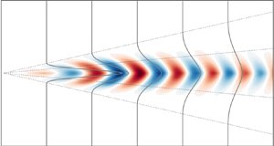
Finally, the three-dimensional spatial structure of the leading SPOD mode of azimuthal wavenumber  $m=1$ is shown in figure 8. It is reconstructed by combining streamwise and cross-stream data and exploiting the self-similar nature of the turbulent flow. A demonstration of the self-similarity of the SPOD modes is shown in the Appendix in figure 18 for
  $m=1$ and figure 19 for
  $m=3$. Further details on the reconstruction of the self-similar wavepacket are also provided in the Appendix. The self-similar wavepacket in figure 8 shows the real part of the three velocity components, where (a) corresponds to the axial component, (b) the radial component and (c) displays the tangential velocity component. As indicated by the two different abscissas, the structure can be represented in terms of the non-dimensional frequency
  $\omega$ or non-dimensional streamwise coordinate
  $\chi$, which are related via the self-similar scaling laws (4.5). The radial coordinate is scaled accordingly as
  $\rho =({r^\ast }/{D})\sqrt {{\omega ^\ast b D}/{A u_0}}$. Hence, the displayed wavepacket represents the fluctuations of the
  $m=1$ mode at any dimensional frequency or spatial location within the flow. On the right in figure 8, the SPOD modes derived from data in the two cross-sections,
  $x=x^\ast /D=50$ and
  $x=x^\ast /D=80$, are displayed at a non-dimensional frequency of
  $\omega =1$ to illustrate their self-similar nature.

Figure 8. Self-similar wavepacket of  $m=1$ mode. Axial (a), radial (b) and tangential (c) velocity components. SPOD modes on the right are shown for
  $\omega =1$ taken at
  $x=x^\ast /D=50$ and
  $x=x^\ast /D=80$, demonstrating the self-similarity of the wavepacket. Black dashed circle marks characteristic length scale
  $r_{1/2}$.
The self-similar representation of the wavepacket clearly reveals spatially growing and decaying regimes in terms of streamwise distance or frequency. The same was already elucidated from the  $m=1$ SPOD spectra (figure 7a). It is further interesting to note that, at short streamwise distance (or low frequencies), where turbulent production is high, the structures are located in the outer region of the jet, while with larger streamwise distance (and higher frequency), the structure decays and is located closer to the jet centre. A detailed description of the growth mechanisms of this structure is not the focus of this work and will be the topic of future work.
5. Linear modelling of coherent structures
In this section, two methods are employed to model the coherent structures in the far field based on the linearized mean-field equations: a local spatial linear stability analysis (LSA) and a local resolvent analysis (RA). Both analyses are based on the measured self-similar mean velocity profile with the mean flow assumed to be quasi-parallel with respect to the axial wavelength of the fluctuations. This holds true for coherent structures at moderate to high frequencies and wavenumbers, which are the main focus of this study.
5.1. Local LSA
For the LSA, the time- and space-dependent flow  $\boldsymbol {u}(\boldsymbol {x},t)$ is decomposed into a time-averaged part
  $\bar {\boldsymbol {u}}(\boldsymbol {x})$, and a fluctuating part
  $\boldsymbol {u}'(\boldsymbol {x},t)$:
 \begin{equation} \boldsymbol{u}(\boldsymbol{x},t)=\bar{\boldsymbol{u}}(\boldsymbol{x})+\boldsymbol{u}'(\boldsymbol{x},t). \end{equation}
For the stability analysis we aim to describe the fluctuating part as normal modes. Therefore, (5.1) is substituted into the full nonlinear equations of motion and the continuity equation for an incompressible isothermal flow, which yields the following set of differential equations in non-dimensional form:
 \begin{gather} \frac{\partial{\boldsymbol{u}'}}{\partial t} + (\boldsymbol{u}' \boldsymbol{\cdot}\boldsymbol{\nabla}) \bar{\boldsymbol{u}} +(\bar{\boldsymbol{u}} \boldsymbol{\cdot}\boldsymbol{\nabla}) \boldsymbol{u}' + \boldsymbol{\nabla} {p}'-\nu \nabla^2 \boldsymbol{u}' ={-}(\boldsymbol{u}' \boldsymbol{\cdot}\boldsymbol{\nabla}) \boldsymbol{u}' + \overline{(\boldsymbol{u}'\boldsymbol{\cdot}\boldsymbol{\nabla}) \boldsymbol{u}'}, \end{gather}
 \begin{gather}\boldsymbol{\nabla}\boldsymbol{\cdot} \boldsymbol{u}' = 0, \end{gather}
with  $\nu =\nu ^\ast / u_{\mathrm cl} r_{1/2}$ as the non-dimensional kinematic viscosity. The first nonlinear term on the right-hand side of (5.2) is neglected due to linearization (
 $(\boldsymbol {u}'\boldsymbol {\cdot }\boldsymbol {\nabla })\boldsymbol {u}'=0$) and the second nonlinear term
  $\overline {(\boldsymbol {u}'\boldsymbol {\cdot }\boldsymbol {\nabla })\boldsymbol {u}'}$ vanishes for frequencies
  $\omega \neq 0$. Furthermore, we employ an eddy viscosity which modifies the linear operator. Based on dimensional considerations, one may assume
  $\nu _t^\ast \sim u_{\mathrm cl} r_{1/2}$, which implies
  $\nu _t$ to be constant in
  $x$ and dependent on
  $r$. For the sake of simplicity, we employ an eddy viscosity that is also constant in
  $r$. A radially dependent eddy viscosity was also tested which only had marginal impact on the results of the LSA (not shown here). The effective
  $\nu _t$ was obtained by a least-square fit of the Boussinesq equation to the measured mean profile and Reynolds stresses according to
 \begin{equation} \nu_t={-}\frac{\overline{u'v'}}{\textrm{d}\bar{u}/\textrm{d} r}, \end{equation}
yielding  $\nu _t=0.0259$, which corresponds to an effective Reynolds number of
  ${Re_{eff}}=\nu _t^{-1}=38.6$. The two orders of magnitudes lower molecular viscosity
  $\nu$ was subsequently neglected for simplicity. The eddy viscosity is incorporated in (5.2) and (5.3), yielding
 \begin{gather} \frac{\partial{\boldsymbol{u}'}}{\partial t} + (\boldsymbol{u}' \boldsymbol{\cdot}\boldsymbol{\nabla}) \bar{\boldsymbol{u}} +(\bar{\boldsymbol{u}} \boldsymbol{\cdot}\boldsymbol{\nabla}) \boldsymbol{u}' + \boldsymbol{\nabla} {p}'-\nu_t \nabla^2 \boldsymbol{u}'=0 \end{gather}
 \begin{gather}\boldsymbol{\nabla}\boldsymbol{\cdot} \boldsymbol{u}' = 0. \end{gather}
For the solution of (5.5) and (5.6) we employ a quasi-parallel spatial stability approach. The fluctuating quantities are expressed as spatially growing or decaying normal modes which are periodic in the axial and azimuthal directions, i.e.
 \begin{gather} {\boldsymbol{u}'}(\boldsymbol{x},t)=\hat{\boldsymbol{u}}(r)\exp({\textrm{i}(\alpha x+ m \theta -\omega t)}) + c.c., \end{gather}
 \begin{gather}{p'}(\boldsymbol{x},t)=\hat{p}(r)\exp({\textrm{i}(\alpha x+ m \theta -\omega t)}) + c.c., \end{gather}
where  $\alpha$ is the complex streamwise wavenumber,
  $\omega$ the real frequency,
  $m$ the real azimuthal wavenumber,
  $\hat {\boldsymbol {u}}$ the complex radial amplitude function and
  $c.c.$ represents the corresponding complex conjugate.
With the normal mode formulation (5.7) and (5.8), (5.5) and (5.6) can be rearranged into an eigenvalue problem
 \begin{equation} \boldsymbol{D}\hat{\boldsymbol{q}}(r)=\alpha \boldsymbol{E} \hat{\boldsymbol{q}}(r), \end{equation}
with complex eigenvalues  $\alpha =\alpha _r+\textrm {i}\alpha _i$ and complex eigenfunctions
  $\hat {\boldsymbol {q}}=[\boldsymbol {\hat u},\hat p]^{\mathrm {T}}$. Within the analysis, homogeneous Dirichlet boundary conditions are set at
  $r\rightarrow \infty$. On the jet axis, the boundary conditions depend on the azimuthal wavenumber
  $m$. All boundary conditions are set in accordance with the method used in Khorrami, Malik & Ash (Reference Khorrami, Malik and Ash1989), which also involves a matrix companion method to reduce the quadratic eigenvalue problem to a linear problem in
  $\alpha$. The resulting eigenvalue problem (5.9) is solved numerically using a spectral method (Khorrami et al. Reference Khorrami, Malik and Ash1989). Detailed explanation about the numerical approach can be found in Oberleithner et al. (Reference Oberleithner, Sieber, Nayeri and Paschereit2011).
To obtain an overall assessment of the linear stability of the mean flow, figure 9(a) depicts the spatial growth rate  $-\alpha _i$ obtained by the LSA for azimuthal wavenumbers ranging from
  $m=0$ to
  $m=5$. The growth rates correspond to those of the leading (least stable) mode at each azimuthal wavenumber and are shown as a function of frequency
  $\omega$. The results reveal that only mode
  $m=1$ is linearly unstable with the neutral point at
  $\omega _n=0.33$. A spatio-temporal analysis was further conducted to ensure that the
  $m=1$ mode is not absolutely unstable (not shown here). All other azimuthal wavenumbers are stable over the entire frequency range. For
  $m\geq 2$, the growth rates of the leading mode continuously decrease with increasing
  $m$. This trend is in line with the SPOD eigenvalue spectrum that shows less pronounced low-rank behaviour for higher azimuthal wavenumbers.

Figure 9. (a) Growth rate  $-\alpha_i$ of least stable eigenmode vs frequency
  $\omega$ for azimuthal wavenumbers
  $m=0$ to
  $m=5$. (b) LSA eigenvalue distribution for
  $m=1$: growth rate
  $-\alpha _i$ vs streamwise wavenumber
  $\alpha _i$ at
  $\omega =0.2$ (unstable) and (c) at
  $\omega=1$ (stable). Colour coding corresponds to the alignment metric
  $\mathcal {M}$ between the first SPOD mode and eigenfunctions from LSA.
To exemplify the LSA results, the eigenvalue spectrum of azimuthal wavenumber  $m=1$ is shown in figure 9(b) at a frequency of
  $\omega =0.2$ (unstable regime) and in figure 9(c) at
  $\omega =1$ (stable regime). Both spectra show several discrete eigenvalues marked by colour coded circles and a continuous spectrum. For
  $\omega =0.2$ two continuous branches merge along
  $\alpha _r \approx 0$ and two continuous branches merge at higher axial wavenumbers that originate at
  $-\alpha _i=2$ and
  $\alpha _r=-2$. The latter two branches strongly depend on the frequency and move outside the shown domain for
  $\omega =1$ (Salwen & Grosch Reference Salwen and Grosch1981; Rodríguez et al. Reference Rodríguez, Cavalieri, Colonius and Jordan2015). The eigenvalues within these branches depend on the numerical discretization and contain core and shear-layer modes, as shown by Rodríguez et al. (Reference Rodríguez, Cavalieri, Colonius and Jordan2015). In contrast, the discrete eigenmodes are numerically converged and reveal, for
  $\omega =0.2$, an unstable mode that is separated from the remaining sub-leading modes. At
  $\omega =1$, the leading mode is also separated from the sub-leading modes but features a negative growth rate, corresponding to a spatially decaying mode. The overall structure of the eigenspectra as shown here is the same for most frequencies and azimuthal wavenumbers considered in this work, with a clear separation of continuous and discrete modes, even at very high frequencies where the discrete modes are strongly damped. Only at near-zero frequencies is it found that the discrete modes interfere with the third and fourth continuous branches.
In order to assess the congruence of the LSA eigenspectrum with the SPOD modes, the discrete modes are colour coded with an alignment metric  $\mathcal {M}$. It is defined as (Cavalieri et al. Reference Cavalieri, Rodríguez, Jordan, Colonius and Gervais2013)
 \begin{equation} \mathcal{M}=\frac{|\left\langle \hat{\boldsymbol{u}}_{m,\omega}, \boldsymbol{a}^1_{m,\omega}\right\rangle|}{\left\|\hat{\boldsymbol{u}}_{m,\omega}\right\| \left\| \boldsymbol{a}^1_{m,\omega}\right\|}, \end{equation}
where the mode shapes are weighted by the radial coordinate  $r$ and
  $\langle \cdot , \cdot \rangle$ denotes the inner product between the weighted mode shapes from LSA and the first SPOD mode and
  $\|\cdot \|$ denotes the corresponding Euclidean norm. A value of
  $\mathcal {M}=1$ indicates perfect alignment between the LSA eigenfunctions and the first SPOD mode while
  $\mathcal {M}=0$ corresponds to completely uncorrelated mode shapes. As shown in figure 9(b,c) for both frequencies, the leading mode agrees very well with the first SPOD mode. In the unstable regime (
 $\omega =0.2$), the second least stable eigenvalue is also in fairly good agreement with the first SPOD mode. In contrast, the leading mode in the stable regime (
 $\omega =1$) is the only mode that shows excellent alignment with the empirical mode. The dominance of the leading mode in relation to the sub-leading modes can be interpreted as a low-rank behaviour of the LSA modes. This behaviour applies to a wide frequency and azimuthal wavenumber range, as will be demonstrated in the following.
Figure 10 shows the alignment between the first SPOD mode and the five leading LSA modes for various frequencies and azimuthal mode numbers. The congruence between the first SPOD and leading LSA mode of azimuthal wavenumber  $m=0$, shown in the top row of figure 10(a), is excellent over a wide range of frequencies. However, the agreement drops at low and very high frequencies. At low frequencies, the third least stable mode (third row) is in better agreement with the empirical mode shapes. For
  $m=0$ the second and fourth least stable modes are only weakly correlated with the SPOD modes with values of
  $\mathcal {M}<0.2$. The poor alignment of these eigenmodes with the first SPOD mode is reasonable since the second and fourth least stable LSA modes represent shear-layer modes which are uncorrelated with the first
  $m=0$ SPOD mode that represents a core mode. The blank areas in the second, fourth and fifth lines correspond to regions where the eigenvalues could not be distinguished from one another properly. For azimuthal wavenumber
  $m=1$, the leading LSA mode is in excellent agreement with the empirical modes up to the highest resolved frequencies. At the lower end of the resolved frequency range, the leading LSA mode does not represent the first SPOD mode and neither is any sub-leading mode in agreement with the empirical modes. Thus, the leading LSA mode shows dominant low-rank behaviour over almost the entire frequency range except for very low frequencies. The blank areas in the alignment contours of the fourth and fifth least stable modes in figure 10(b) are again due to difficulties in tracking the eigenvalues due to their interference with the continuous spectrum. For azimuthal wavenumber
  $m=2$, the leading LSA mode is in very good agreement with the first SPOD mode over the entire frequency range and additionally the second leading mode is in good agreement at low frequencies. Higher azimuthal wavenumbers
  $m>2$ generally feature very similar trends as observed for
  $m=2$. In summary, at mid-range to high frequencies, the empirical mode shapes of all azimuthal wavenumbers are represented very well solely by the leading LSA mode which is clearly prominent in terms of alignment and separation from the sub-dominant modes. This also holds for high azimuthal wavenumbers and frequencies where the growth rate is negative and very low.

Figure 10. Alignment between first SPOD mode and five least stable LSA modes. Alignment of leading mode is shown in the top row and subsequent modes below.
For a visual comparison with the experiments, the LSA mode shapes for azimuthal wavenumber  $m=1$ are shown in figure 11(a) along with the first SPOD mode (b). The displayed mode shapes correspond to the tangential velocity component and are shown at five discrete frequencies. The black dashed circle marks the location of the half-width radius
  $r=1$. As observed in the alignment metric in figure 10(b), the match between the LSA and SPOD modes is very good for a large frequency range, except for the lowest displayed frequency of
  $\omega =0.1$. In figure 11(c), the normalized magnitudes of axial
  $u$, radial
  $v$ and tangential
  $w$ velocity components are shown at a frequency of
  $\omega =1$. The velocity is normalized such that the energy norm (
 $\int _0^\infty (|u|^2+|v|^2+|w|^2)r\, \textrm {d} r$) for SPOD and LSA modes equals 1. In figure 12 the same plot is shown for an azimuthal wavenumber of
  $m=3$. As quantified in figure 10(c) for
  $m=2$ (which is also applicable for
  $m>2$), very good agreement between the LSA and SPOD mode shapes are observed over the entire resolved frequency range.

Figure 11. Mode shapes of tangential velocity component from LSA (a) and SPOD (b) at several frequencies for  $m=1$. Black dashed circle marks characteristic length scale
  $r_{1/2}$. (c) displays normalized magnitudes of axial, radial and tangential velocity components at
  $\omega =1$. Solid lines correspond to LSA results and dashed lines represent SPOD modes.

Figure 12. Mode shapes of tangential velocity component from LSA (a) and SPOD (b) at several frequencies for  $m=3$. Black dashed circle marks characteristic length scale
  $r_{1/2}$. (c) displays normalized magnitudes of axial, radial and tangential velocity components at
  $\omega =1$. Solid lines correspond to LSA results and dashed lines represent SPOD modes.
5.2. Local resolvent analysis
LSA predicts the mean flow to be linearly stable for all modes except for the  $m=1$ mode at low frequencies. However, SPOD reveals low-rank dynamics for structures within a wide frequency and wavenumber range that correlates very well with discrete but stable LSA modes. The occurrence of coherent structures in the flow that are in line with strongly damped stable LSA eigenmodes suggests that the empirical modes are driven by nonlinear forcing which cannot be accounted for by the LSA. This calls for a resolvent analysis (RA) that is capable of determining the optimal response modes in linearly stable flows.
RA is carried out in a local framework following the approach of McKeon & Sharma (Reference McKeon and Sharma2010) with the addition of an eddy viscosity model. In accordance with the LSA, the linear operator is modified by introducing a constant eddy viscosity  $\nu _t=0.0259$ and the remaining nonlinearities are cast into a forcing term
  $\boldsymbol {f}$ that is interpreted as intrinsic turbulent forcing. The resulting system of equations reads
 \begin{gather} \frac{\partial{\boldsymbol{u}'}}{\partial t} + (\boldsymbol{u}' \boldsymbol{\cdot}\boldsymbol{\nabla}) \bar{\boldsymbol{u}} +(\bar{\boldsymbol{u}} \boldsymbol{\cdot}\boldsymbol{\nabla})\boldsymbol{u}' + \boldsymbol{\nabla} {p}' -\nu_t \nabla^2\boldsymbol{u}'=\boldsymbol{f}'. \end{gather}
 \begin{gather}\boldsymbol{\nabla}\boldsymbol{\cdot} \boldsymbol{u}' = 0. \end{gather}
As for the LSA, a normal mode ansatz is introduced. This ansatz applies to both response and forcing modes
 \begin{gather} {\boldsymbol{u}'}(\boldsymbol{x},t)=\hat{\boldsymbol{u}}(r)\exp({\textrm{i}(\alpha_r x+ m \theta -\omega t)}) \end{gather}
 \begin{gather}{p'}(\boldsymbol{x},t)=\hat{p}(r)\exp({\textrm{i}(\alpha_r x+ m \theta -\omega t)}) \end{gather}
 \begin{gather}{\boldsymbol{f}'}(\boldsymbol{x},t)=\hat{\boldsymbol{f}}(r)\exp({\textrm{i}(\alpha_r x+ m \theta -\omega t)}). \end{gather}
Here,  $\alpha _r$ is a real axial wavenumber,
  $\omega$ a real frequency and
  $m$ the real azimuthal wavenumber.
By introducing these ansatz functions, (5.11) and (5.12) can be reformulated as
 \begin{equation} \hat{\boldsymbol{q}}=\boldsymbol{C}(-\textrm{i} \omega \boldsymbol{I} - \boldsymbol{L})^{{-}1} \boldsymbol{B}\hat{\boldsymbol{f}} = \mathcal{H}\hat{\boldsymbol{f}}, \end{equation}
where  $\mathcal {H}$ refers to the resolvent operator. The resolvent analysis constitutes an optimization problem whereby the optimization parameter is the gain defined as
 \begin{equation} \sigma^2=\frac{\left\| \tilde{\boldsymbol{\varPsi}} \right\|^2}{\left\| \tilde{\boldsymbol{\varPhi}} \right\|^2}. \end{equation}
Here,  $\tilde {\boldsymbol {\varPhi }}$ and
  $\tilde {\boldsymbol {\varPsi }}$ correspond to forcing and response modes, respectively. The norm in (5.17) is defined as the
  $L_2$ norm. The optimal response modes
  $\widehat {\boldsymbol {\varPsi }_i}$ and forcing modes
  $\widehat {\boldsymbol {\varPhi }_i}$ form an orthonormal basis and are obtained by a singular value decomposition of the resolvent operator
  $\mathcal {H}$. A system is called to be of low rank, if the gain assigned to the optimal mode is significantly higher than the remaining ones.
Within the present study, the linear operators in (5.16) are constructed via an finite element method (FEM)-based formulation following the procedure of Kaiser, Lesshafft & Oberleithner (Reference Kaiser, Lesshafft and Oberleithner2019). Analogous to the LSA approach, homogeneous Dirichlet boundary conditions are set at  $r\rightarrow \infty$ and the boundary conditions on the jet axis depend on the azimuthal wavenumber.
In figure 13, the optimal and sub-optimal resolvent gains are shown as a function of the axial wavenumber  $\alpha _r$ at a selected frequency of
  $\omega =1$. For the three shown azimuthal wavenumbers, a peak in the resolvent gain curves is observed, which flattens with increasing azimuthal wavenumber, and the gap between the optimal and first sub-optimal mode decreases. These trends are qualitatively in line with the growth rates
  $-\alpha _i$ from LSA, which continuously decrease with increasing
  $m$ for
  $m>1$.

Figure 13. Gain  $\sigma$ vs axial wavenumber
  $\alpha _r$ at
  $\omega =1$ for
  $m=1$,
  $m=2$ and
  $m=3$. Gain of the optimal mode is plotted in black and the subsequent 9 sub-optimal modes are plotted in grey scale in sequential order.
In order to compare the results of the RA with the SPOD modes, an axial wavenumber  $\alpha _r$ has to be selected for each frequency
  $\omega$. Within the present study, the axial wavenumber associated with the largest gain is selected, which corresponds approximately to the point of maximum alignment between the SPOD and RA mode. Figure 14 shows the resulting resolvent gain curves
  $\sigma$ for the optimal and subsequent sub-optimal response modes as a function of frequency. The trends observed in figure 13 are even more pronounced in this representation. For
  $m=1$, a very large gap between the gain of the optimal and first sub-optimal mode can be observed almost over the entire frequency range. Only at very high frequencies does the low-rank behaviour diminish. Furthermore,
  $m=1$ is the only azimuthal wavenumber for which a distinct peak in the gain spectrum is observed. The gain of the optimal mode peaks at
  $\omega =0.33$. This corresponds to the neutral point determined from LSA. At this point, the resolvent gain is infinite by definition. In the unstable regime at frequencies below
  $\omega =0.33$, the RA is not properly defined and neither the gain nor respective mode shapes are considered fully reliable. As the present analysis targets a broad range of frequencies and azimuthal wavenumbers, the inconsistency in this small frequency range appears acceptable. For
  $m>1$ the gain of the optimal mode continuously decreases with increasing frequency and azimuthal wavenumber. Furthermore, the gain separation between the optimal and sub-optimal modes decreases, showing less pronounced low-rank behaviour.

Figure 14. Gain  $\sigma$ vs
  $\omega$ for
  $m=1$,
  $m=2$ and
  $m=3$ for optimal (black) and following 9 sub-optimal modes (grey scale) in sequential order. Axial wavenumber
  $\alpha _r$ corresponds at each frequency
  $\omega$ to the wavenumber associated with the largest gain.
To assess the congruence between RA and the empirical modes, the alignment between the first five SPOD modes and corresponding five RA modes is shown in figure 15 for three azimuthal wavenumbers. The alignment between the first SPOD and optimal RA mode for  $m=0,1,2$ shows very similar trends as for the least-stable LSA mode shown in figure 10. Again, the agreement is excellent over the entire frequency range, except at very low frequencies for
  $m=0$ and
  $m=1$ and at very high frequencies for
  $m=0$. Interestingly, the very good agreement in the high frequency regime is also present where the RA gain curves cannot be considered low rank. The alignment between the sub-optimal RA and SPOD modes is relatively weak throughout, except for
  $m=0$, where a slight increase in correlation towards lower frequencies is observable. The same applies to the sub-optimal RA modes for
  $m=1$ around
  $\omega =0.4$. However, note that the sub-leading SPOD modes are substantially less energetic than the leading one, and the correlations are noisy and inconclusive.

Figure 15. Alignment between first five SPOD modes and five optimal and sub-optimal RA modes. Alignment of the optimal mode is shown in the top row and subsequent modes below.
Overall, SPOD, LSA and RA show consistent characteristics. All three methods indicate low-rank behaviour of the flow dynamics over a wide frequency and azimuthal wavenumber range. From the empirical prospective, the azimuthal wavenumber  $m=1$ is the most energetic and the SPOD mode shows the most pronounced low-rank behaviour. The LSA reveals a corresponding single eigenmode that is the least stable compared to all other azimuthal wavenumbers. Likewise, the RA reveals the largest gain and most pronounced low-rank behaviour. For higher frequencies and azimuthal wavenumbers, a reduction in SPOD mode energy and SPOD and RA low-rank behaviour is observed, which goes along with the more stable LSA modes.
5.3. Accuracy of linear models in the context of turbulent scales
Since both modelling approaches, LSA and RA, show good agreement with the empirical modes, we seek to relate them to the scales of the turbulent spectrum. Furthermore, the congruence and discrepancies between the two models is assessed to potentially identify mechanisms governing the far field dynamics.
To generally classify the turbulent scales resolved in this study, the empirical and analytical data are presented as a function of the axial wavenumber. For the empirical data, a wavenumber spectrum is determined from a spatial Fourier transform of the SPIV data taken in streamwise sections of the flow, following the method proposed by Wänström (Reference Wänström2009). On the jet axis, the wavenumber spectrum reduces to
 \begin{equation} \boldsymbol{\hat{u}}(\kappa) = \int_{\xi}{\boldsymbol{u}'(\xi)\,\textrm{e}^{-\textrm{i} \kappa \xi}\,\textrm{d}\xi}, \end{equation}
where  $\xi =\ln (x-x_0)$ is the logarithmically scaled axial coordinate as proposed by Ewing et al. (Reference Ewing, Frohnapfel, George, Pedersen and Westerweel2007) and
  $\kappa$ the corresponding non-dimensional axial wavenumber. The latter is related to
  $\alpha _r$, with
  $\alpha _r=b \kappa$ and
  $b$ being the jet spreading rate. The fluctuating velocity
  $\boldsymbol {u}'$ in (5.18) is normalized by
  $u_{cl}$. Based on the wavenumber spectra, the spectral density estimates are determined for the axial normal stresses
  $\varPsi _{uu}$ according to
 \begin{equation} \varPsi_{uu}(\alpha_r) = \frac{1}{2{\rm \pi}}\overline{{\hat{u}^{{{\dagger}}}(\alpha_r) \hat{u}(\alpha_r)}}, \end{equation}
and respectively for the radial normal stresses  $\varPsi _{vv}$.
In figure 16(a) the derived spectral density estimates are shown. From the shape of the wavenumber spectrum, the turbulent scales can be classified in the outer productive range with strong anisotropic turbulence ( $\alpha _r<4$) and the inner scales that behave nearly isotropic, characterized by the
  ${\alpha _r}^{-5/3}$ slope, which is characteristic of the inertial subrange. The approximate isotropy of the turbulent scales is also indicated by the equality of the axial and radial normal stresses. The increase of the energy at very high frequencies/wavenumbers is due to the noise floor of SPIV. Overall, the spectrum shows that the scales resolved by SPIV reach far into the inertial subrange.

Figure 16. (a) spectral density estimates from spatial Fourier analysis on jet axis. Markers in (a) represent an estimate of the highest resolved axial, radial and tangential wavenumbers associated with the first SPOD mode for  $m=5$. (b) dispersion relation for
  $m=0$ to
  $m=5$ for LSA (solid) and RA (dashed).
In order to display the LSA and RA modes as a function of the axial wavenumber, the dispersion relation is required, which is shown in figure 16(b). The solid lines correspond to the LSA results and are directly derived from the least stable LSA mode. The dashed lines represent the RA results, which correspond to the axial wavenumber associated with maximum gain (refer to figure 13). The LSA and RA dispersion relations agree generally very well.
To assess the LSA- and RA-based modelling with respect to the turbulent scales, the alignment metrics (5.10) between the leading LSA and optimal RA modes and the first SPOD mode are displayed in figures 17(a) and 17(b), respectively, as a function of the axial wavenumber for azimuthal wavenumbers  $m=0$ to
  $m=5$. Both types of analyses show strikingly similar trends. Particularly for axial wavenumbers higher than
  $\alpha _r=4$, which are associated with the inertial subrange in the averaged turbulent spectrum, a surprisingly good correlation between both models and the first SPOD modes is observed. A slight deterioration of the alignment at the upper end of the wavenumber range can be attributed to aliasing effects/the PIV noise floor that affects the turbulent spectrum. The discrepancies between models and empirical modes at higher wavenumbers for
  $m=0$ seem to be of a physical nature.

Figure 17. Alignment of mode  $m=0$ (top) to
  $m=5$ (bottom) of first SPOD mode and leading mode from LSA (a) and for first SPOD mode and optimal response mode from RA (b). Alignment between leading LSA mode and optimal RA mode is shown in (c).
As the SPOD modes are anisotropic, their axial wavenumber is not necessarily the same as the radial and azimuthal wavenumbers. In fact, as can be inferred from figure 12, the SPOD and analytic modes feature lower radial and azimuthal wavenumbers in comparison to the axial wavenumbers. To account for this, the dominant radial and tangential wavenumbers of the first SPOD mode are estimated from the shape of the  $m=5$ mode at a frequency of
  $\omega =10$, which corresponds to the mode with the smallest scale resolved. The wavelength in radial direction is estimated by visually inspecting the shape of the radial and tangential velocity components in dependence on the radial coordinate. The wavelength in the azimuthal direction is evaluated at the radial location where the radial and tangential velocity magnitudes reach their peak values, which approximately coincide. The resulting wavenumbers are
  $\alpha _{rad}=2{\rm \pi} /\lambda _{{rad}}\approx 5.24$ and
  $\alpha _{tang}=2{\rm \pi} /\lambda _{tang}\approx 5$. The axial wavenumber is determined from LSA as
  $\alpha _{{ax}}=\alpha _r=10.1$. All three values are indicated by yellow markers in figure 16(a). It shows that, although the radial and tangential wavenumbers are lower than the axial wavenumber, all three scales reach into the inertial subrange.
The comparison of the length scales of the leading SPOD mode with the turbulent spectrum allows for a number of observations. Even for the highest resolved frequencies, the first SPOD mode yields non-negligible production and anisotropic structures (confirmed by figure 7). Meanwhile, an increase in isotropic turbulence is reflected by a weakening of the low-rank behaviour of the SPOD modes. Thus, the small-scale isotropic structures associated with the inertial subrange must primarily be represented by subdominant SPOD modes which are neither captured by sub-optimal RA modes (see figure 15) nor by sub-leading LSA modes (not shown here). Nevertheless, the comparison with turbulent scales shows that both RA and LSA are capable of successfully modelling a remarkably large range of frequencies in the jet far field.
In a study by Sasaki et al. (Reference Sasaki, Cavalieri, Jordan, Schmidt, Colonius and Brès2017), high frequency wavepackets were modelled based on parabolized stability equations (PSE) in the jet near field for  $m=0$ to
  $m=4$. In this study, very good agreement in the alignment was reported between the leading PSE mode and SPOD mode, which was obtained in the full spatial domain. This applied to a very wide frequency range and all investigated azimuthal wavenumbers. However, high values of alignment were only found in the spatially unstable regime and the alignment deteriorated quickly in the decaying regime. These contrasting findings with regard to stable modes at high frequencies may be explained by the following aspects of the fully developed turbulence in the jet far field. First, in the present study, an eddy viscosity model is used that is known to work well in the jet far field. Second, the modelled coherent structures show positive production throughout the entire frequency range, which links them to the mean field. This is not necessarily the case for the jet near field. Potentially, this explains why linear models based on the mean flow capture such a wide range of the far field dynamics.
Since both modelling approaches, LSA and RA, yield very similar values in the alignment with the first SPOD mode over a very wide range of turbulent scales, we seek to determine congruence and discrepancies between the two models.
In figure 17(c) the alignment between the least stable LSA and optimal response modes are shown. Astonishingly, the alignment for low and moderate azimuthal and axial wavenumbers is almost perfect. In this regime, the resolvent gains associated with the optimal mode show low-rank behaviour and the LSA growth rate is not too far from zero. Those conditions typically result in a strong agreement between LSA and RA (Beneddine et al. Reference Beneddine, Sipp, Arnault, Dandois and Lesshafft2016; Symon et al. Reference Symon, Rosenberg, Dawson and McKeon2018) unless a pseudo-resonant mechanism (based on non-normality of the linear operator) is present.
Interestingly, figure 17(c) indicates that, for azimuthal wavenumbers  $m\geq 3$, the alignment between each model and the first SPOD mode is better than the alignment between the two models. This results from the radial position of maximum velocity fluctuation magnitude that differs between the models. In relation to the first SPOD mode, the LSA eigenfunctions are centred slightly closer to the jet axis whereas the resolvent modes are located further away from the jet axis.
Despite the small difference between the modelling results, very good agreement between both models and the empirical modes is obtained for higher azimuthal and streamwise wavenumbers. This is also true for the high wavenumber regime, where the LSA predicts strongly decaying modes and where the RA modes do not feature low-rank behaviour. The good match between LSA and RA strongly hints toward a predominantly resonant stability mechanism with negligible pseudo-resonant amplification (Symon et al. Reference Symon, Rosenberg, Dawson and McKeon2018).
Figure 17(a,b) further shows a deviation of both models from the empirical SPOD modes at low axial wavenumbers for  $m=0$ and
  $m=1$. This deviation may be linked to non-parallel flow effects that are relevant at very low axial and azimuthal wavenumbers. This is supported by the work of Mullyadzhanov et al. (Reference Mullyadzhanov, Yavorsky and Oberleithner2019), where a local (or quasi-global) LSA of the Landau jet was performed in spherical coordinates which takes the non-parallel base flow into account. They observed strong deviations from a local quasi-parallel approach for modes
  $m=0$ and
  $m=1$ at low frequencies that are associated with high axial wavelengths, while the results converged for high frequencies and corresponding short axial wavelengths. This suggests that the current mismatch at low frequencies observed for
  $m=1$ and
  $m=0$ is attributed to non-parallel flow effects rather than non-modal stability mechanisms.
On a more general note, discrepancies between the two modelling approaches can also stem from the eddy viscosity model employed in the analysis. The LSA was found to be very robust towards small changes in the eddy viscosity, whereas the local RA reacted quite sensitively, which leaves room for further improvement.
6. Conclusions
The self-similar region of an axisymmetric turbulent jet at a Reynolds number  ${Re}_D=17\,000$ was experimentally investigated by means of time-resolved stereoscopic particle image velocimetry. The two-dimensional-three-component (2D-3C) velocity data allowed the resolution of a large range of turbulent scales reaching far into the inertial subrange. The key goal of the present study was to extract self-similar coherent structures in the mid to high wavenumber/frequency regime and compare them with models from linearized mean-field stability theory. To this end, SPOD was employed to decompose the velocity fields into coherent structures with different azimuthal wavenumbers and frequencies. For the modelling, LSA and RA were carried out in a local parallel framework based on the self-similar mean flow profiles and a simple eddy viscosity model to modify the linear operator.
It was shown that the presented dataset follows consistently self-similar scaling laws in terms of centreline velocity, velocity half-width radius, mean field, Reynolds stresses and turbulent spectra. Furthermore, we provided evidence that the wavepackets observed in this jet flow also scale according to similarity theory.
The modes extracted via SPOD show low-rank behaviour over a wide frequency range and for all azimuthal wavenumbers considered in this study. Mode  $m=1$ features the most pronounced low-rank dynamics, which persists up to the top end of the resolved frequency range. Considering the turbulent production of the leading SPOD modes, all azimuthal wavenumbers, except for
  $m=0$, feature positive values throughout the entire resolved frequency range. For moderate to high frequencies, the total turbulent production is dominated by the first SPOD mode. This indicates that, in this frequency range, the first SPOD mode captures the anisotropic part of turbulence, which extracts energy from the mean flow, whereas the subsequent SPOD modes represent isotropic turbulent structures.
The empirical SPOD modes were compared to analytical modes based on mean field stability theory. A classical local stability analysis was conducted, which determined that only  $m=\pm 1$ is linearly unstable, whereas all other azimuthal wavenumbers
  $m$ were found to be stable. Unexpectedly, even for very high frequencies and azimuthal wavenumbers where all eigenmodes are strongly damped, a single discrete least stable eigenvalue could be identified that correlates very well with the first SPOD mode.
Analogous to LSA, the RA gain spectrum shows pronounced low-rank behaviour for a wide range of frequencies and excellent agreement with the SPOD. Unexpectedly, the agreement is also excellent at very high frequencies and wavenumbers where neither the RA nor the SPOD show low-rank behaviour. The RA further shows the exceptional role of mode  $m=1$, with the most pronounced low-rank behaviour also at very high frequencies.
In conclusion, both linear analyses, LSA and RA, yield modes that are in very good agreement with the empirical SPOD modes even in regimes where the LSA predicts stable strongly damped modes and the RA modes do not feature low-rank behaviour. Thus, the linear analysis based on the mean field captures the dynamics in terms of eigenmodes (LSA) and optimal response modes (RA), however, the nonlinear forcing that drives the empirical modes cannot be considered by the LSA, which predicts strongly negative growth rates. The congruence between LSA and RA modes suggests that the amplification mechanism of the coherent structures is predominantly resonant where non-normality only plays a subordinate role. Discrepancies in the alignment between the empirical SPOD modes and modelled modes at low frequencies for  $m=0$ and
  $m=1$ are likely to be attributable to non-parallel flow effects.
The current work shows that mean flow LSA and RA are capable of modelling a large part of the broadband dynamics of self-similar jet turbulence. In terms of the considered azimuthal wavenumbers,  $m=0$ to
  $m=\pm 5$ capture approximately 77 % of the total turbulent kinetic energy in the jet far field. With respect to the turbulent spectrum, good agreement of the modelled modes with the empirical SPOD modes is obtained up to the highest resolved frequencies, which reach into the inertial subrange of the turbulent spectrum. Furthermore, no substantial deterioration of the modelling quality is observed in this range.
Based on these observations, we hypothesize that the validity of mean-field-based models in self-similar turbulent jets over such a wide frequency range and for decaying stable modes can be attributed to three main factors. First, we use an eddy viscosity model which is known to work well in the far field. Second, due to self-similar scaling the eddy viscosity is constant in the axial direction, and also for all frequencies. Third, the turbulent production is positive in the entire resolved frequency range (except for  $m=0$). Hence, energy is transferred from the mean flow to the coherent structures, establishing a connection between the mean field and the mean-field-based models in a very wide frequency range.
Funding
The authors would like to acknowledge the research funding by the Australian Government through the Australian Research Council, The Australia-Germany Joint Research Cooperation Scheme an initiative of Universities Australia and the German Academic Exchange Service (DAAD). P.K. was supported by a scholarship within the doctoral student's program of the German Academic Exchange Service (DAAD).
Declaration of interests
The authors report no conflict of interest.
Appendix. Reconstruction of self-similar wavepacket
We seek to extract a wavepacket representation of the coherent structures that follow self-similar scaling laws. In this section, the procedure for how we reconstruct such a three-dimensional wavepacket for azimuthal mode  $m=\pm 1$ is presented, along with evidence for the self-similar scaling of these wavepackets. Within this process, all acquired data from streamwise and cross-stream sections of the flow are taken into account, as visualized in figure 2.
The three-dimensional reconstruction of the  $m=\pm 1$ mode is performed in self-similar coordinates according to the following procedure: overall, three quantities are required. The first two quantities are obtained via SPOD from cross-stream data; the radial amplitude distribution (
 $|\hat {\boldsymbol {u}}(r)|$,
  $|\hat {\boldsymbol {v}}(r)|$,
  $|\hat {\boldsymbol {w}}(r)|$) and the radial phase angle (
 $\arg \{\hat {\boldsymbol {u}}(r)\}$,
  $\arg \{\hat {\boldsymbol {v}}(r)\}$,
  $\arg \{\hat {\boldsymbol {w}}(r)\}$) in dependence on
  $\omega$ serve as a basis for the wavepacket reconstruction. To obtain smooth amplitude and phase angle distributions, data from both cross-stream measurement domains (
 $x=50$ and
  $x=80$) are processed individually and averaged subsequently. A comparison of
  $m=1$ mode shapes from the two cross-stream sections is shown in figure 18 to illustrate the self-similarity of SPOD modes. In addition, the same plot is shown for
  $m=3$ in figure 19. As a third quantity in the three-dimensional reconstruction, a relation between self-similar phase velocity
  $c_{ph}=c_{ph}^\ast /u_{\mathrm cl}$ on the jet axis and frequency
  $\omega$ is required.
The phase velocity can be extracted for mode  $m=\pm 1$ from streamwise measurement domains by the procedure illustrated in figure 20. As a first step, each snapshot is decomposed into fluctuations that are symmetric and antisymmetric with respect to the jet centreline. In a streamwise section of the flow, mode
  $m=\pm 1$ is represented by antisymmetric fluctuations, therefore, we only consider these velocity fluctuations in all three velocity components. Please note that the illustrated decomposition in step 1 in figure 20(a) displays the axial and transverse (instead of radial) components and omits the tangential component for the sake of brevity.
As a second step, we perform an SPOD (see figure 20b) based on this conditioned dataset. The resulting SPOD modes are expected to correspond mainly to mode  $m=\pm 1$ because this is the most dominant antisymmetric mode and can be identified by the non-zero velocity fluctuation of the radial/transverse component on the jet axis, as shown in figure 20(b). A comparison of the radial amplitude distribution from streamwise and cross-stream data, as well as frequency spectra, confirms this assumption (not shown here).
As a third step, we extract the phase angle  $\phi$ on the jet axis from the first SPOD mode at each dimensional frequency
  $\omega ^\ast$ (see figure 20c). For the extraction, the radial/transverse velocity component
  $\hat {v}$ is chosen since the corresponding phase angle distribution is fairly constant along the radius. In figure 20(c) the extracted phase angle is shown in dependence on
  $x^\ast$ for various frequencies.
In step four, a streamwise wavenumber is calculated from the extracted phase angle for each frequency mode. This quantity can be transferred into self-similar coordinates, reading  $\alpha _r=({\textrm {d}\phi }/{{\textrm {d}x}^\ast })r_{1/2}$. It is shown in figure 21 for all frequency modes plotted against
  $\omega$. The second axis on top marks the self-similar streamwise coordinate
  $\chi$. Accordingly, the streamwise wavenumbers of all extracted wavepackets determined at different frequencies collapse to a single curve when plotted in a self-similar fashion.

Figure 18. Mode shapes of axial ( $\hat {u}$), radial (
 $\hat {v}$) and tangential (
 $\hat {w}$) velocity components for
  $m=1$ at frequencies
  $\omega =0.5$ (a,c) and
  $\omega =1.5$ (b,d). (a,b) Show data from cross-section
  $x=50$ and (c,d) from
  $x=80$. Velocity components are normalized by the maximum of the axial component. Black dashed circle marks characteristic length scale
  $r_{1/2}$.

Figure 19. Mode shapes of axial ( $\hat {u}$), radial (
 $\hat {v}$) and tangential (
 $\hat {w}$) velocity components for
  $m=3$ at frequencies
  $\omega =0.5$ (a,c) and
  $\omega =1.5$ (b,d). (a,b) Show data from cross-section
  $x=50$ and (c,d) from
  $x=80$. Velocity components are normalized by the maximum of the axial component. Black dashed circle marks characteristic length scale
  $r_{1/2}$.

Figure 20. Schematic of the extraction of self-similar wavenumber  $\alpha _r$ from streamwise data for the reconstruction of wavepackets.

Figure 21. Self-similar wavenumber  $\alpha _r$ for
  $m=1$ extracted from streamwise flow data. Dimensional frequency
  $\omega ^\ast$ increases with lighter colours. Red dashed line marks fit with
  $\alpha _r=1.524\,{\omega }^{0.7205}$.
For  $m=\pm 1$, we can now reconstruct a wavepacket that scales in accordance with similarity theory. Since the SPOD modes are not as distinct at higher frequencies, the extracted phase angles are somewhat noisy. This results in a wavy pattern of the wavenumber
  $\alpha _r$, as seen in figure 21. In order to obtain smooth results for the wavepacket reconstruction, the data are approximated by the analytic expression
  $\alpha _r=1.524\,{\omega }^{0.7205}$, which is also shown as a red line in figure 21. Both investigated axial domains (
 $35<x<74$ and
  $48<x<95$) result in the same self-similar wavenumber
  $\alpha _r$, which corroborates the self-similar state of the flow and the validity of this approach to extract this information from streamwise data. The self-similar phase velocity is then calculated according to
  $c_{ph}={c_{ph}^\ast }/{u_{cl}}={\omega }/{\alpha _r}=0.6562\,{\omega }^{0.2795}$ and the wavelength is derived by
  $\lambda ={2 {\rm \pi}}/{\alpha _r}$.
Up to this point in the analysis, the self-similar scaling of the wavepacket was an assumption based on the self-similarity of the statistical quantities and turbulent spectra. The fact that the determined wavenumber  $\alpha _r$ can be transferred from an axial dependence to a dependence on
  $\omega$ justifies this assumption a posteriori.


