


1. Introduction
Liquid metal blankets have been believed to be the most promising candidates (Abdou et al. Reference Abdou, Morley, Smolentsev, Ying, Malang, Rowcliffe and Ulrickson2015) for the blanket design of future fusion reactors due to their three key functions with heat exchangers, radiation shields and tritium breeders operating at the same time. Liquid metals as used in tritium breeding or cooling would circulate in all kinds of pipes and ducts for different blanket designs such as the water cooled, helium cooled lead lithium blankets (Forest et al. Reference Forest2020; Ling & Wang Reference Ling and Wang2020) and the dual coolant lead lithium blanket (Smolentsev et al. Reference Smolentsev, Morley, Abdou and Malang2015). Magnetohydrodynamic (MHD) interactions (Molokov, Moreau & Moffatt Reference Molokov, Moreau and Moffatt2007) would occur when the electrically conducting liquid metal moves in a strong magnetic field that confines the fusion plasma. One of the open issues in the liquid blanket development is to assess the influence of MHD effects on the fluid dynamics and heat transfer mechanisms (Smolentsev et al. Reference Smolentsev, Moreau, Bühler and Mistrangelo2010; Mistrangelo et al. Reference Mistrangelo, Bühler, Smolentsev, Klüber, Maione and Aubert2021). Under strong magnetic fields, MHD interactions generally result in significant anisotropy of the flow distribution and complex hydrodynamic behaviour. Without considering the thermal effect, on the one hand, the magnetic field can lead to a change of laminar–turbulent transition mechanism (Moffatt Reference Moffatt1967; Davidson Reference Davidson1995; Zikanov et al. Reference Zikanov, Krasnov, Boeck, Thess and Rossi2014) in MHD flows. The magnetic field usually tends to suppress the production of turbulence and make the transition from laminar flow to turbulence occur at much higher Reynolds number (Shatrov & Gerbeth Reference Shatrov and Gerbeth2010). On the other hand, many specific spatial structures such as shear layers (Lehnert Reference Lehnert1952), inflexion points (Kakutani Reference Kakutani1964) and jets (Hunt Reference Hunt1965) may appear in MHD flows due to the action of the magnetic field, and can produce instabilities of free shear flow type such as the sidewall jet-induced instability (Priede, Aleksandrova & Molokov Reference Priede, Aleksandrova and Molokov2010, Reference Priede, Aleksandrova and Molokov2012; Priede, Arlt & Bühler Reference Priede, Arlt and Bühler2015). The critical Reynolds number of jet-induced instability has been revealed to be significantly lower than the Reynolds numbers at which turbulence is observed in experiments (Moresco & Alboussire Reference Moresco and Alboussire2004) or direct numerical simulations (Kinet, Knaepen & Molokov Reference Kinet, Knaepen and Molokov2009).
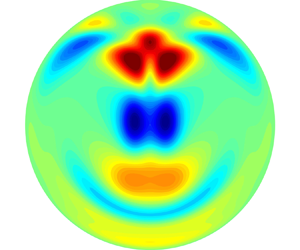
In liquid metal blankets of magnetic-confinement nuclear fusion reactors, mixed convection of liquid metals in pipes or ducts is one of the primary flows due to the extreme conditions of large heat flux and strong magnetic field. Such mixed convection flows have been revealed to be complex and counterintuitive in a lot of laboratory experiments and numerical simulations. In the normal cases of strong magnetic field without heat flux, there exists a laminar–turbulent transition (Zikanov et al. Reference Zikanov, Krasnov, Boeck, Thess and Rossi2014) with the known range  $200 < Re/Ha < 400$ for typical values of the non-dimensional parameters (the Reynolds (
 $Re$) and Hartmann (
 $Ha$) numbers) with respect to isothermal duct, pipe and channel flows of various liquid metal blankets. However, in the experiments of Genin et al. (Reference Genin, Zhilin, Ivochkin, Razuvanov, Belyaev, Listratov and Sviridov2011) and Belyaev et al. (Reference Belyaev, Ivochkin, Listratov, Razuvanov and Sviridov2015) for liquid metal flows in a heated horizontal tube under a transverse horizontal magnetic field, unexpected anomalous temperature fluctuations with low frequency and high amplitude are discovered for strong magnetic fields which occur at
  $Re/Ha < 200$ when the turbulence is usually regarded to be fully suppressed. Large-amplitude low-frequency pulsations of temperature in the form of isolated bursts or quasi-regular fluctuations have also been observed in experiments (Melnikov et al. Reference Melnikov, Sviridov, Sviridov and Razuvanov2014, Reference Melnikov, Sviridov, Sviridov and Razuvanov2016; Kirillov et al. Reference Kirillov, Obukhov, Genin, Sviridov, Razuvanov, Batenin, Belyaev, Poddubnyi and Yu Pyatnitskaya2016; Listratov et al. Reference Listratov, Melnikov, Razuvanov, Sviridov and Zikanov2016; Belyaev et al. Reference Belyaev, Krasnov, Kolesnikov, Biryukov, Chernysh, Zikanov and Listratov2020) of a downward flow in a vertical round pipe and rectangular duct with one wall heated and an imposed strong magnetic field. The high-amplitude low-frequency fluctuations of velocity and temperature that appear in flows with strong convection and magnetic field effects are proposed to be called magneto-convective fluctuations (Belyaev et al. Reference Belyaev, Sardov, Melnikov and Frick2021). Magneto-convective fluctuations obviously have a key impact on the design of the liquid metal blankets of future nuclear fusion reactors and relevant magneto-convection flows have been recently reviewed by Zikanov et al. (Reference Zikanov, Belyaev, Listratov, Frick, Razuvanov and Sardov2021).
To study hydrodynamical stabilities of the MHD mixed convections in the horizontal or vertical duct, the quasi-two-dimensional (Q2-D) model proposed by Sommeria & Moreau (Reference Sommeria and Moreau1982) is usually adopted. Through the Q2-D model, Smolentsev, Vetcha & Moreau (Reference Smolentsev, Vetcha and Moreau2012) first studied instabilities and transitions in MHD duct flows with a symmetric ‘M-shaped’ velocity profile by imposing an external flow-opposing force. Various instability modes and transition scenarios have been revealed by varying this external force and the position of the inflection point. Vetcha et al. (Reference Vetcha, Smolentsev, Abdou and Moreau2013) considered upward flows in a vertical rectangular duct subject to a volumetric heating and a strong transverse magnetic field. Both bulk instability associated with the inflection point and sidewall boundary layer instability are predicted by their linear stability analysis. Vo, Pothérat & Sheard (Reference Vo, Pothérat and Sheard2017) investigated the linear stability of horizontal Poiseuille–Rayleigh–Bénard flows subjected to a transverse magnetic field and a vertical temperature gradient. Liu & Zikanov (Reference Liu and Zikanov2015) further investigated the elevator convection mode for the vertical downward flow using the Q2-D model. Furthermore, numerical simulations of the MHD mixed convection are performed on the Q2-D model. For example, Zhang & Zikanov (Reference Zhang and Zikanov2018) numerically investigated the stabilities of the downward flow in a vertical duct with one heated and three thermally insulated walls under a strong transverse magnetic field. The Q2-D model is originally proposed in the limit of high interaction parameter ( $Ha^2/Re \gg 1$) and Hartmann number (
 $Ha \gg 1$). Thus, it is not suitable to study hydrodynamic stabilities of MHD duct flows in the full physical parameter space, especially to detect the instability boundary when the unstable threshold occurs at a much lower interaction parameter and Hartmann number. Even at high Hartmann number, for the mixed convection in a horizontal duct with imposed transverse horizontal magnetic field, the applicability of the Q2-D model is not a priori certain due to the numerical discovery of the large-scale coherent structure (Zhang & Zikanov Reference Zhang and Zikanov2014) which has significant flow and variations of temperature along the magnetic field lines at the high Grashof regime. Furthermore, the full linear stability analysis of the horizontal MHD mixed convection has revealed that the instability thresholds of the steady solutions with symmetrical or asymmetrical rolls occur at much lower Hartmann number and Grashof number (Hu Reference Hu2020). This clearly shows that the Q2-D model is not appropriate for research on the occurrence process or mechanism of stabilities of the mixed thermal MHD convections in the horizontal duct. Meanwhile, it is also noticed that the Q2-D model is only suitable for the rectangular cross-section duct and then is not available to the circular cross-section pipe. These further shows its limitation of application for general cross-sectional geometries.
Without using the Q2-D model, there exist two other approaches to study MHD mixed convections in horizontal or vertical channels (ducts or pipes). One is direct numerical simulation (Ni et al. Reference Ni, Munipalli, Morley, Huang and Abdou2007), the other is linear global stability analysis (Theofilis Reference Theofilis2011). In order to explain the slow high-amplitude fluctuations of temperature appearing in the experiment of Genin et al. (Reference Genin, Zhilin, Ivochkin, Razuvanov, Belyaev, Listratov and Sviridov2011), Zikanov, Listratov & Sviridov (Reference Zikanov, Listratov and Sviridov2013) conducted a linear stability analysis with direct numerical simulations for the liquid metal mixed convection in a horizontal pipe which is subject to constant flux heating in the lower half with and an imposed transverse magnetic field. Coherent Q2-D rolls aligned with the magnetic field are successfully found at a magnetic field strength far exceeding the laminarization threshold, and transport of the rolls by the mean flow can be used to explain the experimental phenomenon of low-frequency high-amplitude fluctuations of temperature. Through similar numerical approaches, Zhang & Zikanov (Reference Zhang and Zikanov2014) further analysed the liquid metal mixed convection in a horizontal duct with bottom heating and transverse magnetic field. The same coherent Q2-D rolls are found in the ‘low- $Gr$’ regime, while a combination of spanwise rolls and streamwise-oriented rolls is revealed in the ‘high-
 $Gr$’ regime. The linear exponential growth rates are computed as functions of streamwise wavelength for both symmetrical and asymmetrical steady rolls, meanwhile, the spatial structure of instability modes is exhibited during the stage of exponential growth. Their main conclusion is that the instability leading to the formation of convection rolls aligned with the magnetic field is a common feature of the flow invariably observed at
  $Ha > 200$ and sufficiently high
  $Gr$. Zikanov & Listratov (Reference Zikanov and Listratov2016) further performed numerical simulations of the downward flow of a liquid metal in a vertical pipe and attributed the large-amplitude fluctuations of temperature to the growth and quasi-periodic breakdown of the pairs of ascending and descending jets related to the elevator modes. Based on the approach of linear global stability analysis, Hu (Reference Hu2020) first studied the linear stabilities of the symmetrical and asymmetrical steady solutions of a similar MHD mixed convection to that of Zhang & Zikanov (Reference Zhang and Zikanov2014) in a horizontal duct. It is much easier to obtain the linear critical stability boundary curves for both symmetrical and asymmetrical steady solutions. Through these boundary curves, it is revealed that their 3-D oscillatory instabilities occur at large magnetic fields and buoyancy is the dominant destabilizing term from energy budget analyses. These can explain the results of the experiments of Belyaev et al. (Reference Belyaev, Ivochkin, Listratov, Razuvanov and Sviridov2015) that temperature fluctuations disappear under moderately strong magnetic fields, while high-amplitude low-frequency oscillations reappear under a much stronger magnetic field through a linear instability transition process. Recently, Hu (Reference Hu2021) further analysed linear global stabilities of a downward flow of liquid metal in a vertical duct under strong wall heating and a transverse magnetic field. Three-dimensional elevator and oscillatory unstable modes are revealed through the eigenspectrum computation. The elevator mode is found to be always unstable and independent of the basic flow profile. The unstable oscillatory mode is directly related to the basic upward reverse flow and first occurs at the specific flow structure which has an upward reverse flow near the heating wall and a downward flow near the opposite wall. The shear Kelvin–Helmholtz instability due to the existence of an inflection point is found to be the key instability mechanism of the 3-D oscillatory mode through energy budget analyses. Then, it is concluded that the appearance of the unstable oscillatory mode may be regarded as an alternative physical explanation for the high-amplitude, low-frequency pulsations of temperature in the experiments and related numerical simulations.
Direct numerical simulations have been demonstrated to be an important approach for the hydrodynamical stability of the liquid metal MHD mixed convection in a horizontal pipe (Zikanov et al. Reference Zikanov, Listratov and Sviridov2013). However, on one hand, it is difficult to determine the stability boundary of the MHD mixed convection for large Hartmann numbers through direct numerical simulations due to considerable computational overhead for each set of parameters. On the other hand, it is not clear why natural thermogravitational convection becomes a dominant destabilization mechanism, which only is regarded as a hypothesis through a flow visualization of physical experiments or numerical simulations. It is easy to solve the above two difficulties through the linear global stability analysis, which has been reviewed comprehensively by Theofilis (Reference Theofilis2011). Linear global stability analysis is mainly based on the solution of the multi-dimensional eigenvalue and has many successful applications, especially for non-parallel and 3-D flows (Theofilis Reference Theofilis2003). In this paper, full linear global stability analyses without using the Q2-D approximation for the MHD mixed convection flows in a circular pipe have been performed successfully. Through the eigenvalue computation of linear global stability equations with the finite-element method, the critical linear stability boundaries of the MHD mixed convection can be plotted in the parameter plane of the Hartmann number and Grashof number. The critical boundary for moderate Hartmann number is determined by the unstable mode which was first found by Zikanov et al. (Reference Zikanov, Listratov and Sviridov2013) through direct numerical simulations. The other critical boundaries for small Hartmann number are also given and determined by different most unstable modes. At the critical points on these stability boundaries, energy budget analyses are further performed to study the destabilization mechanism of the corresponding unstable modes. In order to study the spatio-temporal structures of nonlinear MHD mixed convection close to the stability boundary curves, direct numerical simulations with the Fourier-spectral finite-difference method are performed using a modified Openpipeflow Navier–Stokes solver. It will be seen from these simulations that much more complex spatio-temporal structures would appear when the simulation parameters get farther and farther away from the stability boundary. Furthermore, the initial condition dependence of numerical simulations is also considered for these complex nonlinear states.
2. Physical model and governing equations
2.1. Physical model
The physical model comes from Genin's experiment and considers a liquid metal flow along a horizontal electrically insulating pipe subject to bottom uniform heating with heat flux intensity  $q$ and an external constant transverse magnetic field
  $\boldsymbol {B}_0$, as shown in figure 1. Mixed convection flow would be produced by a combined action of a pressure driven flow and thermal buoyancy due to huge temperature gradients with strong magnetic fields, then such a flow is usually called MHD mixed convection. The liquid metal is not a magnetizable liquid and is considered as an incompressible, electrically conducting Newtonian viscous fluid with constant kinematic viscosity
  $\nu$, electric conductivity
  $\sigma$ and thermal conductivity
  $\kappa$. The pipe wall is assumed to be electrically insulating, the upper half of the wall is assumed to be thermally insulating and the lower half of the wall has an imposed constant and uniform heat flux.

Figure 1. The flow configuration. The pipe is placed horizontally and heated from below with a constant heat flux  $q$, and the upper half of the pipe wall is assumed to be insulated. Uniform magnetic field
  $\boldsymbol B$ is imposed in the transverse horizontal direction and gravity field
  $\boldsymbol g$ has a vertical downward direction.
The Oberbeck–Boussinesq approximation is applied for the buoyancy force and the quasi-static model is adopted for the electromagnetic interactions. Then the dimensional governing equations for the liquid metal pipe flow can be described by the Navier–Stokes system
 \begin{gather} \boldsymbol{\nabla} \boldsymbol{\cdot} {\boldsymbol{v}} = 0, \end{gather}
 \begin{gather} \rho_0\left[\frac{\partial {\boldsymbol{v}}}{\partial t} + {\boldsymbol{v}} \boldsymbol{\cdot} \boldsymbol{\nabla} {\boldsymbol{v}}\right] ={-} \boldsymbol{\nabla} p + \rho_0\nu \nabla^2 {\boldsymbol{v}} + \boldsymbol{F}_b + \boldsymbol{F}_l, \end{gather}
 \begin{gather} \rho_0 c_p \left[\frac{\partial T}{\partial t} + {\boldsymbol{v}} \boldsymbol{\cdot} \boldsymbol{\nabla} T\right] = \boldsymbol{\nabla} \boldsymbol{\cdot} (\kappa \boldsymbol{\nabla} T) + \frac{1}{\sigma}{\boldsymbol{j}}^2 + \varPhi + Q. \end{gather}
Here,  ${\boldsymbol {v}}$,
  $p$ and
  $T$ are the fields of velocity, pressure and temperature,
  $\rho _0$ is the reference value of the fluid mass density,
  $c_p$ is the specific heat capacity,
  $({1}/{\sigma }){\boldsymbol {j}}^2$ is the loss of magnetic energy due to Joule dissipation,
  $\varPhi$ is the loss of kinetic energy due to viscous dissipation and
  $Q$ is other sources of volumetric energy release such as nuclear radiation or chemical reactions. The buoyancy force
  $\boldsymbol {F}_b$ with the Oberbeck–Boussinesq approximation is assumed to vary linearly with temperature and is represented as
 \begin{equation} \boldsymbol{F}_b =(\rho-\rho_0)\boldsymbol{g},\quad \rho = \rho_0\left[1-\beta(T-T_0) \right], \end{equation}
where  $\beta$ is the thermal expansion coefficient and
  $\boldsymbol {g}$ is the gravitational acceleration in the negative vertical direction. The Lorentz force
  $\boldsymbol {F}_l$ with the quasi-static model is represented as
 \begin{gather} \boldsymbol{F}_l = {\boldsymbol{j}}\times \boldsymbol{B}_0, \end{gather}
 \begin{gather} {\boldsymbol{j}} = \sigma\left( -\boldsymbol{\nabla}\phi + {\boldsymbol{v}}\times \boldsymbol{B}_0 \right), \end{gather}
where  ${\boldsymbol {j}}$ is the induced electric current density,
  $\phi$ is the electrostatic potential. It is clearly seen that, using the quasi-static model, the induced magnetic field can be neglected and the magnetic field remains undisturbed in the expressions of the Lorentz force (2.5) and Ohm's law (2.6). The quasi-static model has been proven to be sufficiently accurate when the magnetic Reynolds and Prandtl numbers are both small (Roberts Reference Roberts1967; Davidson Reference Davidson2001). In most laboratory experiments, the magnetic Reynolds number is relatively small and the induced magnetic field is much weaker than the imposed field.
The current density can be considered to be solenoidal by neglecting displacement currents and assuming the fluid to be electrically neutral, i.e.
 \begin{equation} \boldsymbol{\nabla}\boldsymbol{\cdot}{\boldsymbol{j}}=0. \end{equation}
Then by substituting the Ohm's law into above solenoidal relation, a Poisson equation for the electrostatic potential is obtained as follows
 \begin{equation} \nabla^2 \phi = \boldsymbol{\nabla} \boldsymbol{\cdot} ( {\boldsymbol{v}}\times \boldsymbol{B}_0 ) . \end{equation}
By neglecting all energy dissipation and other energy sources except the Fourier diffusion term, the temperature equation (2.3) is reduced to
 \begin{equation} \frac{\partial T}{\partial t} + {\boldsymbol{v}} \boldsymbol{\cdot} \boldsymbol{\nabla} T = \chi \nabla^2 T . \end{equation}
Here,  $\chi =\kappa /\rho _0 c_p$ is the thermal diffusivity.
The boundary conditions on the lower half of the wall include the no-slip condition for the velocity and constant heat flux for the temperature, i.e.
 \begin{equation} \kappa \frac{\partial T}{\partial n} = q, \end{equation}
and the boundary conditions on the upper half of the wall are no slip and thermally insulated, i.e.
 \begin{equation} \frac{\partial T}{\partial n} = 0. \end{equation}
2.2. Model non-dimensionalization and reduction
The dimensional governing equations can be further non-dimensionalized by using the pipe diameter  $d$ as the length scale, mean streamwise velocity
  $U_m$ as the velocity scale,
  $qd/\kappa$ as the temperature scale,
  $B_0$ as the scale of the magnetic field strength and
  $dB_0U_m$ as the scale of the electric potential. Then the dimensionless governing equations can be written as
 \begin{gather} \frac{\partial {\boldsymbol{v}}}{\partial t} + {\boldsymbol{v}} \boldsymbol{\cdot} \boldsymbol{\nabla} {\boldsymbol{v}} ={-}\boldsymbol{\nabla} p + \frac{1}{Re} \nabla^2 {\boldsymbol{v}} + \boldsymbol{f}_b + \boldsymbol{f}_l, \end{gather}
 \begin{gather} \boldsymbol{\nabla} \boldsymbol{\cdot} {\boldsymbol{v}} = 0, \end{gather}
 \begin{gather} \frac{\partial T}{\partial t} + {\boldsymbol{v}} \boldsymbol{\cdot} \boldsymbol{\nabla} T = \frac{1}{Pe} \nabla^2 T . \end{gather}
The buoyancy and Lorentz forces are dimensionalized as
 \begin{equation} \boldsymbol{f}_b = \frac{Gr}{Re^2}T \boldsymbol{e}_y \quad \text{and} \quad \boldsymbol{f}_l = \frac{Ha^2}{Re} {\boldsymbol{j}}\times \boldsymbol{e}_x, \end{equation}
where the dimensionless parameters including the Reynolds number, Prandtl number, Péclet number, Grashof number and Hartmann number are defined as
 \begin{gather} Re= \frac{U_m d}{\nu},\quad Pr=\frac{\nu}{\chi}, \quad Pe = \frac{U_m d}{\chi}=Re\cdot Pr, \end{gather}
 \begin{gather} Gr = \frac{g\beta qd^4}{\nu^2\kappa},\quad Ha = B_0 d\left(\frac{\sigma}{\rho\nu}\right)^{1/2}. \end{gather}
In order to compare our results with those of Zikanov et al. (Reference Zikanov, Listratov and Sviridov2013), the same dimensionless parameters for the Reynolds number and Prandtl number are selected, with  $Re=9046$ and
  $Pr=0.022$ in this work.
The boundary conditions at the pipe wall include the no-slip conditions for velocity and the condition of perfect electric insulation
 \begin{equation} {\boldsymbol{v}} = 0,\quad \frac{\partial \phi}{\partial r}=0, \quad \text{at}\ r=\sqrt{x^2+y^2}=1/2. \end{equation}
Here,  $x$ and
  $y$ are horizontal and vertical coordinates in the cross-section, respectively. For the temperature, the condition on the lower half of the wall is
 \begin{equation} \frac{\partial T}{\partial r}=1, \quad \text{at}\ r=1/2, \end{equation}
while for the upper thermally insulating half of the wall we have
 \begin{equation} \frac{\partial T}{\partial r}=0, \quad \text{at}\ r=1/2. \end{equation}
The temperature field can be further decomposed as a sum of the mean mixed temperature and the resulting temperature deviation
 \begin{equation} T(\boldsymbol{x},t) = T_m(z) + \theta(\boldsymbol{x},t). \end{equation}
The mean mixed temperature is assumed to be a linear function of the streamwise coordinate  $z$, which makes the overall energy balance between the heat transfer across the lower half of the wall with constant heat flux and the streamwise convection heat transfer. Then its streamwise gradient is given by
 \begin{equation} \frac{{\rm d}T_m}{{\rm d}z} = \frac{\texttt{P}}{A\cdot Pe}, \end{equation}
where  $\texttt {P}={\rm \pi} /2$ is the perimeter of the heated portion of the wall and
  $A={\rm \pi} /4$ is the cross-sectional area of the pipe. Then the temperature governing equation is written as
 \begin{equation} \frac{\partial \theta}{\partial t} + {\boldsymbol{v}} \boldsymbol{\cdot} \boldsymbol{\nabla} \theta = \frac{1}{Pe} \nabla^2 \theta - w \frac{{\rm d}T_m}{{\rm d}z}. \end{equation}
The pressure can also be decomposed into three parts as follows:
 \begin{equation} p= \tilde{p}(z) + \breve{p}(y,z) + p(\boldsymbol{x},t). \end{equation}
The first part is a linear function of  $z$ corresponding to a spatially uniform streamwise gradient
  ${\rm d}\tilde {p}/{\rm d}z$ which pushes the pipe flow. The second part is used to balance with the buoyancy force from the mean mixed temperature
 \begin{equation} \breve{p}(y,z) = \frac{Gr}{Re^2}y\, T_m + {\rm cons.} \end{equation}
Also, the forcing in the streamwise direction from the second part is deduced with
 \begin{equation} \frac{\partial\breve{p}}{\partial z} = \frac{Gr}{Re^2}\frac{{\rm d}T_m}{{\rm d}z} y. \end{equation}
We look for the 2-D steady-state solutions in which the velocity, pressure, temperature (excluding the linear part coming from the bottom heating) and electrostatic potential are independent of streamwise coordinate, as follows:
 \begin{gather} {\boldsymbol{v}}_b = {\boldsymbol{V}}(x,y) = (\boldsymbol{U}(x,y),W(x,y)), \end{gather}
 \begin{gather} p=P(x,y),\quad \theta=\varTheta(x,y),\quad \phi = \varPhi(x,y). \end{gather}
Here,  $\boldsymbol{U}=(U,V)$ is the cross-sectional velocity, and
  $W$ is the streamwise velocity. Thus the 2-D steady governing systems for the steady flow state are obtained as follows:
 \begin{gather} (\boldsymbol{U}\boldsymbol{\cdot}\boldsymbol{\nabla}_s)W={-}{\rm d}\tilde{p}/{\rm d}z - \frac{Gr}{Re^2}\frac{{\rm d}T_m}{{\rm d}z} y +\frac{1}{Re}\boldsymbol{\nabla}_s^2 W + \frac{Ha^2}{Re} F_z, \end{gather}
 \begin{gather} (\boldsymbol{U}\boldsymbol{\cdot}\boldsymbol{\nabla}_s)\boldsymbol{U}={-}\boldsymbol{\nabla}_s P +\frac{1}{Re}\boldsymbol{\nabla}_s^2 \boldsymbol{U} + \frac{Gr}{Re^2}\varTheta \boldsymbol{e}_y + \frac{Ha^2}{Re} \boldsymbol{f}, \end{gather}
 \begin{gather} (\boldsymbol{U}\boldsymbol{\cdot}\boldsymbol{\nabla}_s)\varTheta=\frac{1}{Pe}\boldsymbol{\nabla}_s^2 \varTheta -W\frac{{\rm d}T_m}{{\rm d}z}, \end{gather}
 \begin{gather} \boldsymbol{\nabla}_s \boldsymbol{\cdot} \boldsymbol{U} = 0, \end{gather}
 \begin{gather} \boldsymbol{F} = (-\boldsymbol{\nabla} \varPhi + {\boldsymbol{v}}_b \times \boldsymbol{e}_x)\times \boldsymbol{e}_x, \end{gather}
 \begin{gather} \nabla^2 \varPhi = \boldsymbol{\nabla} \boldsymbol{\cdot} ( {\boldsymbol{v}}_b \times \boldsymbol{e}_x ) . \end{gather}
Here,  $\boldsymbol {\nabla }_s=(\partial _x,\partial _y)$,
  $\boldsymbol{F}=(\boldsymbol{f},F_z)$ and
  $\boldsymbol{f}=(F_x,F_y)$. The corresponding boundary conditions on the walls are the no-slip condition for the velocity
 \begin{equation} {\boldsymbol{v}}_b = 0,\quad \text{at}\ r=1/2, \end{equation}
fixed heat flux for constant-rate heating on the lower half of the wall and thermal insulation on the upper half of the wall
 \begin{gather} \frac{\partial\varTheta}{\partial r} = 1,\quad \text{at}\ r=1/2,\ y<0, \end{gather}
 \begin{gather} \frac{\partial\varTheta}{\partial r} = 0,\quad \text{at}\ r=1/2,\ y>0, \end{gather}
as well as zero current flux due to the electrically insulating walls
 \begin{equation} \frac{\partial\varPhi}{\partial r} = 0,\quad \text{at}\ r=1/2. \end{equation}
3. Numerical methods
3.1. Finite-element method for linear global stability analysis
For linear global stability analysis of the MHD mixed convection in a circular pipe, the 2-D steady-state solutions of the governing equations should be computed. The Taylor–Hood finite-element method is used for spatial discretization for the steady governing equations, and the Newton method is adopted to solve the derived nonlinear system when the cross-sectional velocity is not zero. A high-level integrated software FreeFem++ (Pironneau, Hecht & Morice Reference Pironneau, Hecht and Morice2013) for the numerical solution of nonlinear multiphysics partial differential equations is adopted for the computation of the steady-state solutions. The bi-dimensional anisotropic mesh generator BAMG built into FreeFem++ is used to define the circular cross-section geometry and generate the 2-D triangular meshes. Three borders are first defined for the 2-D mesh generation, one is the outer wall boundary with  $r=0.5$, the other two are internal circles with
  $r=0.4$ and
  $r=0.3$. Then, discrete mesh points are uniformly distributed on these borders with different numbers. The numbers of mesh points can be used to control the mesh resolution and further be defined as
  $n_r$,
  $0.5n_r$ and
  $0.3n_r$, respectively. This will produce a much larger mesh size for the border with the smaller circle radius. It is easily seen from figure 1 that the triangular mesh with
  $n_r=100$ has a much smaller mesh size near the pipe wall. Obviously, finer mesh resolution near the pipe wall is realized and beneficial to improve the numerical accuracy.
Because the mean streamwise velocity is adopted as the velocity scale, it should be noted that the uniform streamwise pressure gradient  ${\rm d}\tilde {p}/{\rm d}z$ should be adjusted to make the average streamwise velocity to be positive one, i.e.
 \begin{equation} \frac{1}{A}\int_A W\, \mathrm{d} A = 1. \end{equation}
A simple bisection process can be used to satisfy relation (3.1). The Newton iterative method needs a good initial guess, then the steady-state solutions are computed continuously from small dimensionless parameters to large ones. In order to verify the correctness of the 2-D steady-state solutions, the same cases as Zikanov et al. (Reference Zikanov, Listratov and Sviridov2013) for  $Re=9046$,
  $Pr=0.022$,
  $Gr = 8.298\times 10^7$ with different Hartmann numbers are considered. Base flow solution of the streamwise velocity and temperature field along the cross-section for
  $Ha=102$ is first plotted in figure 2, which has the same spatial distribution as Zikanov et al. (Reference Zikanov, Listratov and Sviridov2013). A detailed comparison of the profiles of the streamwise velocity
  $W$ of the base flow along horizontal and vertical lines drawn through the pipe axis is presented in figure 3. It is clearly seen from these figures that the steady-state solutions obtained by the finite-element method agree very well with those by direct numerical simulations of Zikanov et al. (Reference Zikanov, Listratov and Sviridov2013).

Figure 2. Base flow solution of the streamwise velocity (a) and temperature (b) field along the cross-section;  $Re=9046$,
  $Pr=0.022$,
  $Gr = 8.298\times 10^7$ and
  $Ha=102$.

Figure 3. Profiles of the streamwise velocity  $W$ of the base flow along horizontal (a) and vertical (b) lines drawn through the pipe axis; solid line is obtained by the finite element method with FreeFem++ software, while triangle symbols are from direct numerical simulations of Zikanov et al. (Reference Zikanov, Listratov and Sviridov2013);
  $Re=9046$,
  $Pr=0.022$,
  $Gr = 8.298\times 10^7$ and
  $Ha=102$.
In order to study the asymptotic behaviour in time of generic small-amplitude perturbations of  $({\boldsymbol {V}}', P', \varTheta ', \varPhi ')$ imposed on the steady-state mixed convection, these perturbations can be expanded as normal modes in the streamwise direction as follows:
 \begin{equation} ({\boldsymbol{V}}', P', \varTheta', \varPhi') = (\hat{{\boldsymbol{v}}}, \hat{p}, \hat{\theta}, \hat{\phi})\exp({\rm i}kz+\gamma t), \end{equation}
where  $k$ is the wavenumber in the streamwise direction, and
  $\gamma =\gamma _r + {\rm i}\gamma _i$ is the corresponding complex growth rate. By substituting the expressions of the disturbed flow field
  ${\boldsymbol {V}} + {\boldsymbol {V}}',P+P',\varTheta +\varTheta ',\varPhi +\varPhi '$ into the governing system, the full global linear stability equations are obtained as follows:
 $$\begin{gather} \gamma \hat{u} +\left( \boldsymbol{U}\boldsymbol{\cdot}\boldsymbol{\nabla}_s + {\rm i}kW \right)\hat{u} +\left( \boldsymbol{\hat{u}}\boldsymbol{\cdot}\boldsymbol{\nabla}_s \right) U ={-}\frac{\partial \hat{p}}{\partial x}\nonumber\\ +\frac{1}{Re}\left(\boldsymbol{\nabla}_s^2-k^2\right)\hat{u}, \end{gather}$$
 $$\begin{gather} \gamma \hat{v} +\left( \boldsymbol{U}\boldsymbol{\cdot}\boldsymbol{\nabla}_s + {\rm i}kW \right)\hat{v} +\left( \boldsymbol{\hat{u}}\boldsymbol{\cdot}\boldsymbol{\nabla}_s \right) V ={-}\frac{\partial \hat{p}}{\partial y}\nonumber\\ +\frac{1}{Re}\left(\boldsymbol{\nabla}_s^2-k^2\right)\hat{v} +\frac{Ha^2}{Re}\left(-{\rm i}k\hat{\phi}-\hat{v} \right), \end{gather}$$
 $$\begin{gather} \gamma \hat{w} +\left( \boldsymbol{U}\boldsymbol{\cdot}\boldsymbol{\nabla}_s + {\rm i}kW \right)\hat{w} +\left( \boldsymbol{\hat{u}}\boldsymbol{\cdot}\boldsymbol{\nabla}_s \right) W ={-}{\rm i}k\hat{p}\nonumber\\ +\frac{1}{Re}\left(\boldsymbol{\nabla}_s^2-k^2\right)\hat{w}+\frac{Gr}{Re^2}\hat{\theta} +\frac{Ha^2}{Re}\left(\frac{\partial\hat{\phi}}{\partial y}-\hat{w} \right), \end{gather}$$
 $$\begin{gather} \gamma \hat{\theta} +\left( \boldsymbol{U}\boldsymbol{\cdot}\boldsymbol{\nabla}_s + {\rm i}kW \right)\hat{\theta} +\left( \boldsymbol{\hat{u}}\boldsymbol{\cdot}\boldsymbol{\nabla}_s \right) \varTheta\nonumber\\ = \frac{1}{Pe}\left(\boldsymbol{\nabla}_s^2-k^2\right)\hat{\theta}-\hat{w}\frac{{\rm d}T_m}{{\rm d}z}, \end{gather}$$
 \begin{gather} \frac{\partial \hat{u}}{\partial x}+\frac{\partial \hat{v}}{\partial y} + {\rm i}k\hat{w} = 0, \end{gather}
 \begin{gather} \left(\boldsymbol{\nabla}_s^2-k^2\right)\hat{\phi} - \left(\frac{\partial\hat{w}}{\partial y}-{\rm i}k\hat{v} \right)=0. \end{gather}
Here,  $\hat {{\boldsymbol {v}}}=(\boldsymbol{\hat {u}},\hat {w})=(\hat {u},\hat {v},\hat {w})$, and the boundary conditions are given by
 \begin{equation} \hat{{\boldsymbol{v}}}=\frac{\partial\hat{\theta}}{\partial r}=\frac{\partial\hat{\phi}}{\partial r} = 0, \quad \text{at}\ r=1/2. \end{equation}
The spatial discretization of Taylor–Hood finite elements can also be used for the global linear stability equations. After the spatial discretization of the linear stability equations, a generalized eigenvalue problem has to be solved in the matrix form as follows:
 \begin{equation} {\boldsymbol{A}}\hat{{\boldsymbol{q}}} = \gamma {\boldsymbol{B}} \hat{{\boldsymbol{q}}}, \end{equation}
where  $\hat {{\boldsymbol {q}}}=(\hat {{\boldsymbol {v}}}, \hat {p}, \hat {\theta }, \hat {\phi })$ is the eigenvector collecting the velocity components, pressure, temperature and electrostatic potential of each degree of freedom of the discrete problem,
  ${\boldsymbol {A}}$ and
  ${\boldsymbol {B}}$ are large sparse complex matrices. In order to facilitate the extraction of the desired eigenvalues for unstable modes, spectral transformations should be introduced into the generalized eigenvalue problem. Theofilis (Reference Theofilis2011) has reviewed a lot of spectral transformations commonly utilized in the global instability analysis of fluid flows. Most commonly used is the shift-and-invert strategy which transforms the generalized eigenvalue problem into a standard eigenvalue problem as follows:
 \begin{equation} ({\boldsymbol{A}}-\mu{\boldsymbol{B}})^{{-}1}{\boldsymbol{B}} \hat{{\boldsymbol{q}}} = (\gamma-\mu)^{{-}1} \hat{{\boldsymbol{q}}}. \end{equation}
The shift matrix can be solved by the UMFPACK or MUMPS sparse LU solver and the standard eigenvalue problem solved with an implicitly restarted Arnoldi algorithm as provided in the ARPACK software library (Lehoucq, Sorensen & Yang Reference Lehoucq, Sorensen and Yang1998). Thus, the largest eigenvalues of the transformed matrix now correspond to those eigenvalues of the original generalized eigenvalue equation which are the closest to the shift value  $\mu$.
In order to validate the computation of the eigenspectrum, the linear growth rate and phase velocity of most unstable mode as a function of wavenumber are plotted in figure 4 for  $Re=9046$,
  $Pr=0.022$,
  $Gr = 8.298\times 10^7$ and
  $Ha=306$. Compared with the numerical simulation results of Zikanov et al. (Reference Zikanov, Listratov and Sviridov2013), it is easily found that the linear growth rates we get from FreeFem++ software are a little higher than their results, this is especially obvious near the maximum growth rate. It is noticed that Zikanov et al. (Reference Zikanov, Listratov and Sviridov2013) used two different streamwise grid numbers, the larger one (
 $N=64$) is for long-wave perturbations while the smaller one (
 $N=32$) is for short-wave perturbations. Under these two mesh resolutions, their phase velocity results of most unstable mode are obviously different, also specifically for moderate wavenumbers (
 $k=5\sim 7$) where large exponential growth occurs. Interestingly, it is found that a good agreement between our eigenspectrum results and numerical simulations of Zikanov et al. (Reference Zikanov, Listratov and Sviridov2013) occurs when the exponential perturbation growth is not very strong.

Figure 4. Linear growth rate (a) and phase velocity (b) of most unstable mode as a function of wavenumber; solid line is obtained by the finite-element method with FreeFem++ software, while rectangle and triangle symbols are from direct numerical simulations of Zikanov et al. (Reference Zikanov, Listratov and Sviridov2013) with respect to the streamwise grid numbers  $N=32$ and
  $N=64$;
  $Re=9046$,
  $Pr=0.022$,
  $Gr = 8.298\times 10^7$ and
  $Ha=306$.
3.2. Fourier-spectral finite-difference method for direct numerical simulation
For direct numerical simulations, we solve the dimensionless governing equations in cylindrical coordinates where  $r,\beta$,
 $z$ denote the radial (i.e. wall-normal), azimuthal and axial directions, respectively. Then, the velocity field would be denoted with
  ${\boldsymbol {v}}=(u_r,u_\beta,u_z)$. We use a Fourier-spectral finite-difference method for discretizing the equations. Field variables, i.e.
  ${\boldsymbol {v}}$,
  $p$,
$p$,  $\phi$ and
  $\theta$, are expanded with a twofold Fourier expansion
 \begin{equation} A(r,\beta,z,t)=\sum_{k={-}K}^{K}\sum_{m={-}M}^{M}\hat A(r,t)_{k,m} \exp{\{{\rm i}k\alpha z+{\rm i}m\beta}\}, \end{equation}
in which  $\hat A(r,t)_{k,m}$ is the Fourier coefficient of the
  $(k,m)$ Fourier mode and is a function of
  $r$ and
  $t$,
$t$,  $\alpha$ would determine spatial periodicity. In the radial direction, we use a 9-stencil high-order finite-difference method for the discretization. The nonlinear terms are calculated using the pseudo-spectral technique with the
  $3/2$-rule for dealiasing. Also,
  $2K$ and
  $2M$ give the total number of Fourier modes used in the axial and azimuthal directions, respectively. We use the finite-difference scheme, the singularity-removal technique at the pipe axis and the message passing interface (MPI) parallelization strategy of OPENPIPEFLOW (Willis Reference Willis2017). In particular, the singularity removal is achieved by avoiding a grid point at the pipe axis
  $r=0$ and imposing proper parity conditions on the velocity, electric potential and temperature in the neighbourhood of the pipe axis. To be clear, near the pipe axis
  $u_r$ and
  $u_\beta$ are odd for even
  $m$ and even for odd
  $m$, whereas
  $u_z$,
  $\phi$ and
  $\theta$ are even for even
  $m$ and are odd for odd
  $m$. Technically, the parity condition is implemented by imposing a homogeneous Dirichlet condition for odd functions and a homogeneous Neumann condition for even functions at
  $r=0$. The details can be found in the documentation of OPENPIPEFLOW (Willis Reference Willis2017).
For the time integration of the Navier–Stokes equations and the heat equation, a semi-implicit three-level Adams–Bashforth time-integration scheme is adopted. Linear terms are treated implicitly and the nonlinear term is treated explicitly using a backward differentiation scheme. The incompressibility condition is imposed using a projection method (Hugues & Randriamampianina Reference Hugues and Randriamampianina1998). Since only the lower half-pipe wall is heated and the upper half-pipe wall is thermally insulated, there will exist a discontinuity with respect to the heat flux  ${\partial T}/{\partial r}$ at the boundary between the heated and insulated parts of the pipe wall. In order to use the Fourier-spectral method, we adopt a steep tanh function to approximate this discontinuity. Assuming the heated part is located at
  $\beta \in [{{\rm \pi} }/{2}, {3{\rm \pi} }/{2}]$, then the distribution of the heat flux around the whole pipe wall is given by
 \begin{equation} q=\dfrac{\partial \theta}{\partial r}(\beta)=0.5-0.5\tanh{\dfrac{|\beta-{\rm \pi}|-\dfrac{\rm \pi}{2}}{\delta}}, \end{equation}
where the parameter  $\delta$ is a control parameter which determines the steepness at the approximated discontinuity boundary. As shown in figure 5, it is clearly seen that smaller parameter
  $\delta$ gives rise to steeper boundary for the heat flux. However, a much smaller parameter
  $\delta$ would need more azimuthal collocation points near the approximated discontinuity boundary and then should be properly chosen to balance the accuracy and computational cost.

Figure 5. The distribution of the heat flux around the whole pipe wall used for direct numerical simulations with the spectral finite-difference method.
As the steady base flow is streamwise invariant, we can choose to only solve the  $k = 0$ modes to obtain the base flow. It is obvious that the base flow would have 2-D stability in the cross-section. As a validation, we compare our calculations using the spectral method with the results using the finite-element method in the previous subsection. The flow parameters of the test case are
  $Ha=204$,
  $Re=9046$,
  $Gr=8.298\times 10^7$,
  $Pr=0.022$. The resolution of the spectral simulation is
  $N=144$ and
  $M=96$ (i.e. 144 grid points on the radius and
  $2M=192$ grid points in the azimuthal direction before dealiasing). The steepness parameter
  $\delta =0.05$ and this azimuthal resolution give approximately six grid points within the smoothing region of the approximated discontinuity of heat flux. Figure 6(a,b) shows the visualization of the base flow in our spectral simulations for the streamwise velocity and temperature field in the cross-section. It is seen that the basic streamwise velocity becomes uniform along the magnetic field direction in the bulk of the circular pipe for large Hartmann numbers. In figure 6(c,d), the streamwise velocity and temperature distributions along the vertical and horizontal lines of the cross-section are compared between our spectral simulation and the finite-element calculation. The agreement between the two sets of results is excellent with a deviation below 0.5 %. This agreement validates our methods and particularly the smoothing of the heat flux in our spectral methods, at least for the base flow calculation.

Figure 6. The base flow calculated using the spectral method and finite-element method. Contours of temperature (a) and streamwise velocity (b) on the pipe cross-section. Data are from our spectral method simulation. (c) Comparison of temperature distribution on the vertical and horizontal lines through the pipe centre. (d) Comparison of streamwise velocity on the vertical and horizontal lines through the pipe centre. In (c,d), symbols are data from our spectral method simulation and lines are from the finite-element simulation.
After obtaining the base flow, we can perturb the base flow with small perturbations in the spectral space, i.e. small Fourier coefficient of a given mode with the wavenumber  $(k\alpha, m)$ is set to give the initial condition of direct numerical simulations. Then, the linear growth rate of the unstable mode at a fixed wavenumber can be calculated from the modal kinetic energy variation between two different time instances, i.e.
 \begin{equation} \gamma=\frac{1}{2}\frac{\log{KE(t_2)}-\log{KE(t_1)}}{t_2-t_1}, \end{equation}
where  $\gamma$ denotes the linear growth rate,
  $KE=\int _V({\boldsymbol {v}}-{\boldsymbol {v}}_b)\,{\rm d}V$ is the modal kinetic energy and
  $t_1$ and
  $t_2$ are two time instants in the exponentially growing stage. The phase speed of the leading eigenmode can be calculated as
 \begin{equation} c=\frac{\lambda}{T}, \end{equation}
with the streamwise wavelength  $\lambda$ and the period of oscillation
  $T$ which can be measured by monitoring the velocity at a fixed point in the flow domain. For the same case with
  $Ha=306$,
  $Re=9046$,
  $Gr=8.298\times 10^7$ and
  $Pr=0.022$ as in Zikanov et al. (Reference Zikanov, Listratov and Sviridov2013), the linear growth rates and phase speeds with respect to different wavenumbers can be computed through both the eigenvalue computation of the linear stability equations and the numerical simulations with the spectral method, as shown in figure 7. Although the two approaches are different and performed independently, it is clearly seen that a good agreement is obtained and can be used as a cross-validation of these two approaches. A further convergence test for the linear growth rate with respect to the steepness parameter
  $\delta$ is given in table 1, which shows
  $\delta =0.5$ with
  $M=96$ can yield good calculation accuracy. An additional validation of our spectral method against an asymptotic solution of the basic flow for the MHD pipe flow (without the heating and buoyancy) can be found in Appendix A. All these tests confirm the correctness of our basic flow calculations.

Figure 7. The linear growth rate (a) and the phase speed (b) of the leading eigenmode with respect to different wavenumbers. Here, the solid line is obtained with the eigenvalue computation of the linear stability equations while discrete circle symbols are the results by direct numerical simulations using the spectral method. The dimensionless parameters  $Ha=306$,
  $Re=9046$,
 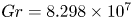 $Gr=8.298\times 10^7$ and
  $Pr=0.022$ are adopted, while the steepness parameter
  $\delta =0.05$ is used for direct numerical simulations.
Table 1. Convergence of the linear growth rate about the smoothing width  $\delta$. The flow parameters are
  $Ha=306$,
  $Re=9046$,
  $Gr=8.298\times 10^7$ and
  $Pr=0.022$, and the streamwise wavelength of
  $\lambda =1.0$ is considered for this convergence test.

4. Linear stability analysis
Although the linear growth rate and phase speed of the most unstable mode have been computed and agree with the results of Zikanov et al. (Reference Zikanov, Listratov and Sviridov2013), there exist two main flow stability questions to answer. The first one is the linear stability boundary of the MHD mixed convection, while the other one regards the flow destabilization mechanism which can deepen our understanding of the underlying physical mechanism.
4.1. Linear stability boundary of the MHD mixed convection
Linear stability boundary of the MHD mixed convection is determined by the most unstable mode, which can be easily computed if there exists only one unstable mode for the parameters under investigation. However, if there exist more than one unstable modes and especially if they have close linear growth rates, then the linear stability boundary may become complex and is difficult to obtain. The critical curves for the linear stability of the MHD mixed convection are first plotted in the  $Gr$–
$Gr$– $Ha$ parameter space with
  $Re=9046$ and
  $Pr=0.022$ as shown figure 8. It is clearly seen that there exist three critical curves located at small and large Hartmann numbers. All the critical curves have been validated by our direct numerical simulations. The critical curve for large Hartmann number is determined by the only unstable mode denoted by mode I, which was first revealed by the numerical simulations of Zikanov et al. (Reference Zikanov, Listratov and Sviridov2013). It is easily found that the unstable mode I occurs above a threshold of the Hartmann number of approximately
  $Ha=136.33$. Across the threshold, the unstable region for the Grashof number becomes larger and larger with the increase of the Hartmann number. The upper boundary of the unstable region increases nearly exponentially while the lower boundary decreases very slowly. The other two critical curves are located at small Hartmann numbers and determined by different unstable modes. They intersect at
  $Ha=37.46$ and are denoted by mode II and mode III, respectively. The critical Grashof number on these two critical curves increases nearly exponentially with the increase of the Hartmann number, from
  $Gr_c\sim 1.2\times 10^6$ at
  $Ha=20$ to
  $Gr_c\sim 1.8\times 10^8$ at
  $Ha=80$. Within the unstable region bounded by the critical curves for the small Hartmann number, there exist many other unstable modes which are not presented here.

Figure 8. The critical curves of the most unstable modes in the  $Gr$–
$Gr$– $Ha$ parameter space with
  $Re=9046$ and
  $Pr=0.022$.
Along all the critical curves of the most unstable modes in the  $Gr$–
$Gr$– $Ha$ parameter space, the corresponding wavenumber and phase speed as a function of Hartmann number can be plotted, as shown in figure 9. It is clearly seen that both the critical wavenumber and phase velocity for small Hartmann numbers are much smaller than those for large Hartmann numbers. Then, for small Hartmann numbers, long-wave instabilities first occur at the threshold, and the critical wavenumber is found to increase with the increase of the Hartmann number. Meanwhile, the phase velocity of these long-wave instabilities even decreases with the increase of the Hartmann number for the unstable mode II. It is also seen that at
  $Ha=67.7$ there exists a jump of the critical wavenumber and phase velocity of mode II. It is carefully checked that this jump is not due to eigenmode transiton, but a rapid change of the critical parameters for the same unstable mode.

Figure 9. Critical wavenumber (a) and phase velocity (b) of most unstable modes along all the critical curves as a function of Hartmann number with  $Re=9046$ and
  $Pr=0.022$.
Spatial structure of the 3-D unstable mode for the perturbations of temperature and vertical velocity in the horizontal cross-section passing through the axis of the pipe is presented in figures 10 and 11 at two critical points with large and small Hartmann numbers, respectively. It is easily seen that the spatial structure for the critical case of  $Ha=136.33$ is very similar to the simulation result by Zikanov et al. (Reference Zikanov, Listratov and Sviridov2013) for
  $Ha = 306$ and
  $\lambda = 1.0$. Specifically, the simulation result for large Hartmann number has a more uniform distribution of vertical velocity along the magnetic field direction. Obviously, there exists only one unstable mode which results in such a similar spatial structure for different large Hartmann numbers. However, the spatial structure for the critical case of
  $Ha=50$ is very different, as shown in figure 11. It is easily seen that the temperature perturbation is distributed near the lateral walls and in the central region, while the perturbations of three velocity components concentrate in the central region. Different spatial structures of different critical eigenmodes imply different destabilization mechanisms, which are further studied in following subsection.

Figure 10. Spatial structure of the 3-D unstable mode for the perturbations of temperature (a) and vertical velocity (b) in the horizontal cross-section passing through the axis of the pipe at a critical point of  $k_c=5.8$,
  $Ha=136.33$,
  $Gr=5.14\times 10^7$,
  $Re=9046$ and
  $Pr=0.022$.

Figure 11. Spatial structure of the 3-D unstable mode for the perturbations of temperature (a), vertical velocity (b) and streamwise velocity (c) in the horizontal cross-section passing through the axis of the pipe at a critical point of  $k_c=1.69$,
  $Ha=50$,
  $Gr=2.898\times 10^7$,
  $Re=9046$ and
  $Pr=0.022$.
4.2. Energy budget analyses at the critical unstable thresholds
In order to obtain the physical destabilization mechanism, it is usual to perform energy budget analyses at the critical thresholds for the most unstable mode. First, the linear stability equations (3.3)–(3.5) are multiplied by the complex conjugate of the velocity perturbation  $\hat {{\boldsymbol {v}}}^*$ and then integrated on the cross-section
  $A$. After some simplifications, an equation giving the rate of change of the fluctuating kinetic energy can be derived. At the critical threshold (
 $\mathrm {Re}(\lambda )=0$) for any unstable mode, kinetic energy budgets can be further obtained as
 \begin{equation} E_{su} + E_{sv} + E_{sw} + E_{b} + E_{m} + E_d = 0, \end{equation}
where  $E_{su}$,
  $E_{sv}$ and
  $E_{sw}$ are the productions of fluctuating kinetic energy by shear of the basic flow,
  $E_{b}$ is the production of fluctuating kinetic energy by buoyancy,
  $E_{m}$ is the dissipation of fluctuating kinetic energy by magnetic forces and
  $E_d$ is the viscous dissipation of fluctuating kinetic energy. They are defined as follows:
 \begin{gather} E_{su} ={-}\mathrm{Re}\left(\int_A \left[\hat{u}\frac{\partial U}{\partial x}\hat{u}^* + \hat{v}\frac{\partial U}{\partial y}\hat{u}^*\right] \,{\rm d}x\,{\rm d}y\right), \end{gather}
 \begin{gather} E_{sv} ={-}\mathrm{Re}\left(\int_A \left[\hat{u}\frac{\partial V}{\partial x}\hat{v}^* + \hat{v}\frac{\partial V}{\partial y}\hat{v}^*\right] \,{\rm d}x\,{\rm d}y\right), \end{gather}
 \begin{gather} E_{sw} ={-}\mathrm{Re}\left(\int_A \left[\hat{u}\frac{\partial W}{\partial x}\hat{w}^* + \hat{v}\frac{\partial W}{\partial y}\hat{w}^*\right] \,{\rm d}x\,{\rm d}y\right), \end{gather}
 \begin{gather} E_{b} = \mathrm{Re}\left(\int_A \frac{Gr}{Re^2}\hat{\theta}\hat{v}^* \,{\rm d}x\,{\rm d}y\right), \end{gather}
 \begin{gather} E_{m} = \mathrm{Re}\left(\int_A \frac{Ha^2}{Re} \left[(-\boldsymbol{\nabla} \hat{\phi} + \hat{{\boldsymbol{v}}} \times \boldsymbol{e}_x)\times \boldsymbol{e}_x\right] \hat{{\boldsymbol{v}}}^* \,{\rm d}x\,{\rm d}y\right), \end{gather}
 \begin{gather} E_{d} ={-}\mathrm{Re}\left(\int_A \frac{1}{Re}\frac{\partial \hat{v}_i}{\partial x_j}\frac{\partial \hat{v}_i^*}{\partial x_j} \,{\rm d}x\,{\rm d}y\right). \end{gather}
All these terms can be further normalized by the viscous dissipation of fluctuating kinetic energy  $E_d$, then a normalized kinetic energy budget equation is written as
 \begin{equation} E'_{su} + E'_{sv} + E'_{sw} + E'_{b} + E'_{m} = 1, \end{equation}
where  $E'_{su}=E_{su}/|E_d|$,
  $E'_{sv}=E_{sv}/|E_d|$,
  $E'_{sw}=E_{sw}/|E_d|$,
  $E'_{b}=E_{b}/|E_d|$,
  $E'_{m}=E_{m}/|E_d|$.
The kinetic energy budgets by shear of the basic flow, buoyancy and magnetic forces at the critical points of the least stable 3-D modes are presented for different Hartmann numbers in table 2. For all cases of mode I, it is easily seen that the production of fluctuating kinetic energy by buoyancy  $E'_{b}$ is the dominant destabilizing term, the production of fluctuating kinetic energy by the streamwise shear of the basic flow
  $E'_{sw}$ gives a significant stabilization effect and the production of fluctuating kinetic energy by the cross-sectional shear of the basic flow
  $E'_{su}$ and
  $E'_{sv}$ is very small and thus has little effect on the flow stability. According to the values of the stabilizing term
  $E'_{m}$, the cases on the lower boundary of mode I have a much weaker stabilization effect due to magnetic forces than those on the upper boundary of mode I. For the cases of mode II and mode III, it is found that the streamwise shear of the basic flow gives the dominant production of fluctuating kinetic energy due to positive large values of
  $E'_{sw}$. Then, the dominant destabilization mechanism is the streamwise shear of the basic flow instead of buoyancy with negligible terms
  $E'_{b}$. It is also found that, with the increase of Hartmann number along the critical curves of mode II and mode III, the values of the destabilization term
  $E'_{su}$ as well as stabilization terms
  $E'_{sv}$ and
  $E'_{m}$ become larger and larger.
Table 2. Kinetic energy budgets by shear of the basic flow  $E'_{su}$,
  $E'_{sv}$,
  $E'_{sw}$, buoyancy
  $E'_{b}$ and magnetic forces
  $E'_{m}$ at the critical point of the most unstable 3-D mode for different Hartmann numbers with
  $Re=5000$ and
  $Pr=0.0321$.

Now the dominant destabilization mechanism is revealed to be buoyancy for mode I as well as streamwise shear of basic flow for mode II and mode III. It is necessary to plot the spatial distribution of local buoyancy and the local streamwise shear of the basic flow i.e. the integral terms in the integral formula (4.4) and (4.5), at the critical points for these modes. As shown in figure 12(a), it is clearly seen that the local buoyancy  $E_b$ for the production of fluctuating kinetic energy is mainly located in the middle and lower parts of the pipe for mode I. However, the local streamwise shear of the basic flow
  $E_{sw}$ for mode II is situated at the upper part of the pipe, as seen in figure 12(b).

Figure 12. Spatial distribution of (a) the local buoyancy  $E_b$ and (b) local streamwise shear of the basic flow
  $E_{sw}$ at the critical points of the 3-D unstable modes for (a) mode I with
  $k_c=5.8$,
  $Ha=136.33$,
  $Gr=5.14\times 10^7$ and (b) mode II with
  $k_c=1.69$,
  $Ha=50$,
  $Gr=2.898\times 10^7$; where
  $Re=9046$ and
  $Pr=0.022$.
5. Nonlinear flow states
According to the stability boundary curves obtained in the previous section, we can further study the nonlinear flow states within the linearly unstable parameter regions through direct numerical simulations. Simulation parameters  $(Ha,Gr)$ selected for this study are shown in figure 13 as symbols, while other parameters are fixed as
  $Re = 9046$ and
  $Pr = 0.022$.

Figure 13. The points in the  $Ha$–
$Ha$– $Gr$ plane considered for DNS analysis:
  $(Ha, Gr)=(45, 2\times 10^7)$ (circle),
  $(40, 2\times 10^7)$ (up-triangle),
  $(30, 2\times 10^7)$ (diamond),
  $(150, 8.298\times 10^7)$ (square),
  $(180, 8.298\times 10^7)$ (plus) and
  $(306, 8.298\times 10^7)$ (right triangle).
5.1. Low- $Ha$ branch

Starting from a point close to the neutral stability boundary at  $(Ha, Gr)=(45, 2\times 10^7)$, we explore horizontally at
  $(Ha, Gr)=(40, 2\times 10^7)$ and
  $(30, 2\times 10^7)$. For all simulations in this subsection, the pipe length is chosen to be 12.2 pipe diameters, which is three times the wavelength of the most unstable mode at
  $(Ha, Gr)=(45, 2\times 10^7)$.
5.1.1. The case $(Ha, Gr)=(45, 2\times 10^7)$

The streamwise velocity fields for the nonlinear flow state and the most unstable mode are both computed by direct numerical simulations and shown in figure 14. It is clearly seen that the nonlinear saturated flow exhibits a travelling wave structure that is symmetric about the vertical plane through the pipe axis. The spatial distributions of the streamwise velocity in all cross-sections are very similar with respect to both the saturated flow state and the most unstable mode. Obviously, the reason is that the nonlinear effect is very weak and the nonlinear flow state is thus dominated by the most unstable mode when the parameters are very close to the linear stability boundary.

Figure 14. The streamwise velocity on the pipe cross-sections at  $(Ha, Gr)=(45, 2\times 10^7)$. The full velocity is plotted in the
  $r$–
$r$– $\beta$ cross-section (a), vertical
  $r$–
$r$– $z$ cross-section (i.e. the
  $y$–
$y$– $z$ plane through the pipe axis) (b) and horizontal
  $r$–
$r$– $z$ cross-section (i.e. the
  $x$–
$x$– $z$ plane through the pipe axis) (c). The deviation with respect to the basic laminar flow is shown in (d–f) and the most unstable linear mode is visualized in (g–i). The location of the maximum deviation of
  $u_z$ from the basic laminar flow is shitted to the left end of the pipe in all the plots in the
  $r$–
$r$– $z$ cross-sections. Panels (a,d,g) are plotted at the left end of the pipe.
5.1.2. The case $(Ha, Gr)=(40, 2\times 10^7)$

At this parameter point, we find that the saturated flow state seems to have a strong dependence on the initial condition. Direct numerical simulations for this case are performed with two different initial conditions. The temporal evolution of the flow is monitored using the kinetic energy  $KE_{3D}=\int _V({\boldsymbol {v}}-<{\boldsymbol {v}}>_z)\,{\rm d}V$ associated with the streamwise dependent velocity components, see figure 15.

Figure 15. The kinetic energy of the 3-D flow components (streamwise dependent ones),  $KE_{3D}$, of two simulations starting from different initial conditions at
  $(Ha, Gr)=(40, 2\times 10^7)$. One starts from a fully turbulent flow simulated at
  $Ha=30$ and the other from a slightly perturbed laminar basic flow, see the blue and red curves, respectively.
The first simulation begins with a fully turbulent state and the kinetic energy  $KE_{3D}$ is plotted as the blue curve in figure 15. The flow remains turbulent for several hundred time units, and then seems to approach a periodic state with large kinetic energy oscillations. Flow fields for the streamwise velocity at four time instants (marked with four symbols in figure 15) are visualized in figure 16. The first two columns correspond to the time instants marked with red circle and green triangle, respectively. Although both of them are at the peaks of the oscillation in
  $KE_{3D}$, the flow field is not identical to that seen in the
  $r$–
$r$– $\beta$ cross-section. Nevertheless, by looking at the flow fields in the vertical and horizontal
  $r$–
$r$– $z$ cross-sections, it can be observed that the two flow fields are nearly identical up to a phase shift. Therefore, the period of the oscillation of
  $KE_{3D}$ is not equal to the period of the flow field. Furthermore, we compare the flow fields of the first column and the fourth column corresponding to the two time instants marked with the red circle and blue square (both are at peaks). These two flow fields seem identical up to a reflection about the vertical plane through the pipe axis. This means that the two flow fields are separated by half a period in phase. Then, it can be inferred that the period of the flow field should correspond to four periods of the oscillation in
  $KE_{3D}$, which is nearly 380 time units. The third column corresponding to the black diamond in figure 15 shows the flow field at the trough of the oscillation in
  $KE_{3D}$, where the velocity perturbations are much weaker than those at other three peak instants. It seems that the periodic state only maintains one cycle, and then the flow begins to leave the periodic orbit after
  $t=1400$ because the oscillation becomes irregular at later times. The temporal evolution of this nonlinear flow state indicates that there exists an unstable nonlinear periodic solution at the given flow parameters.

Figure 16. The quasi-periodic flow state at  $(Ha, Gr)=(40, 2\times 10^7)$. The visualization of the streamwise velocity field at the four time instants marked by the four symbols on the blue curve in figure 15. Each column corresponds to a time instant. Panels (a–l) share the same colour scale. From (a,d,g,j) to (c, f,i,l),
  $r$–
$r$– $\beta$ cross-section at the left end of the pipe, vertical
  $r$–
$r$– $z$ cross-section and horizontal
  $r$–
$r$– $z$ cross-section.
The second simulation starts from random small perturbations and is shown as the red curve in figure 15. It is clearly seen that there is no high-amplitude periodic oscillation up to 1100 time units. The flow field is visualized at  $t=966$ in figure 17. Compared with the first simulation, although there are some similarities in the spatial distributions of the flow fields in the cross-sections, there does not exist any regular or periodic structure in either the signal of
  $KE_{3D}$ or the flow fields visualized in the pipe cross-sections. However, it should be noted that we cannot rule out the possibility that the non-periodic state would also approach some periodic orbits at some time in the future. Both nonlinear states show little similarity in flow structure with the linear eigenmode (which is similar to figure 14g–i).

Figure 17. Visualization of the flow field of the non-periodic flow state at  $(Ha, Gr)=(40, 2\times 10^7)$, which was started from a small random perturbation, see the red curve in figure 15. Data are taken at
  $t=966$. Panels (a–c) to (j–l) show full
  $u_z$, full
  $\theta$,
  $u_z$ deviation and
  $\theta$ deviation, respectively.
5.1.3. The case $(Ha, Gr)=(30, 2\times 10^7)$
When  $Ha$ is further decreased to 30, several different initial conditions are used for direct numerical simulations and the flow evolves into a fully turbulent state in all the cases. The turbulent flow field is visualized in figure 18. The first column shows an instantaneous
  $u_z$ field, and the second column shows the corresponding temperature
  $\theta$ field. One can see that, although the turbulent
  $u_z$ fluctuations (turbulent fluctuation refers to the deviation from the turbulent mean flow, where the turbulent mean flow refers to the flow averaged in time and streamwise direction) seem to be homogeneous in the vertical
  $r$–
$r$– $z$ cross-section, the turbulent temperature
  $\theta$ fluctuations seem to be significant only close to the bottom heated wall. The third column shows the deviation of the mean flow from the basic laminar flow. It can be seen that the mean streamwise velocity is faster than the basic flow mainly close to the top wall, is slower than the basic flow in the middle and only slightly deviates from the basic flow near the bottom wall. The mean temperature is higher than the basic laminar flow mainly near the bottom wall, and only slightly deviates from the basic laminar flow in the upper part of the pipe.

Figure 18. Visualization of the fully turbulent flow field at  $(Ha, Gr)=(30, 2\times 10^7)$. Panels (a–c) show the full
  $u_z$ in the
  $r$–
$r$– $\beta$ cross-section (a), in the vertical
  $r$–
$r$– $z$ cross-section (b) and the turbulent fluctuations of
  $u_z$ in the vertical
  $r$–
$r$– $z$ cross-section (c). Panels (d–f) show the full
  $\theta$ field in the same cross-sections. Panels (g,h) shows the deviation of the turbulent mean of
  $u_z$ and
  $\theta$ with respect to their basic laminar counterparts, respectively.
5.2. High-$Ha$ branch

Within the unstable region of mode I at large  $Ha$, as seen in figure 13, three Hartmann numbers
  $Ha=150$,
  $180$ and
  $306$ with a fixed Grashof number
  $Gr=8.298\times 10^7$ are considered to investigate the nonlinear flow states. Obviously, nonlinear flow states are responsible for the low-frequency high-amplitude fluctuations of temperature appearing in the experiment of Genin et al. (Reference Genin, Zhilin, Ivochkin, Razuvanov, Belyaev, Listratov and Sviridov2011). In order to explain that the high-amplitude fluctuations originally come from the global instability mode, it is necessary to compare the nonlinear flow states with the global unstable eigenmode with respect to the spatial structure of the flow field.
5.2.1. The case $(Ha,Gr)=(150, 8.298\times 10^7)$

This set of parameters is close to the linear stability boundary, and the saturated nonlinear flow state exhibits a nonlinear travelling wave, as shown in figure 19. From the second column of this figure, the amplitude of the deviation  $u_z$ is relatively small and thus indicates that the nonlinear flow field is only slightly deviated from the basic laminar flow. Comparing the deviation of
  $u_z$ with the most unstable linear eigenmode (mode I) in all cross-sections, as shown in the second and third columns, one can see that their spatial distributions are very similar. Therefore, the saturated nonlinear flow is mainly dominated by the most unstable eigenmode and the nonlinearity is too weak to change the spatial structure significantly. This observation is similar to the case with
  $(Ha,Gr)=(45, 2\times 10^7)$, which is close to the linear stability boundary curves of the low-
 $Ha$ branch. However, noticeable differences in the flow field from the case with
  $(Ha,Gr)=(45, 2\times 10^7)$ can be observed. Firstly, the dominant flow structures of the large-
 $Ha$ case have a much larger streamwise wavenumber, i.e. smaller streamwise wavelength. Secondly, the flow structures in the
  $r$–
$r$– $\beta$ cross-section show much simpler symmetrical structures, which are nearly aligned with the magnetic field. Thirdly, the flow structures extend along the whole horizontal pipe cross-section, rather than being localized in a narrow region around the vertical
  $r$–
$r$– $z$ cross-section as in the case with
  $(Ha,Gr)=(45, 2\times 10^7)$.

Figure 19. Visualization of the streamwise velocity field at  $(Ha, Gr)=(150, 8.298\times 10^7)$. Panels (a–c) to (g–i) show the full
  $u_z$,
  $u_z$ deviation and
  $u_z$ of the most unstable eigenmode. From (a,d,g) to (c, f,i),
  $r$–
$r$– $\beta$, vertical
  $r$–
$r$– $z$, and horizontal
  $r$–
$r$– $z$ cross-sections.
5.2.2. The case $(Ha,Gr)=(180, 8.298\times 10^7)$

The case with  $Ha=180$ is farther from the linear stability boundary compared with the
  $Ha=150$ case. The simulation is started with small random perturbations, and strong temporal oscillations in
  $KE_{3D}$ are observed when the flow develops into a nonlinear state, as shown in figure 20. The flow fields at three time instants between the trough and peak of an oscillation (see the symbols in figure 20) are visualized in figure 21. While the high-amplitude oscillation of
  $KE_{3D}$ is temporally quasi-periodic, the spatial structure of flow flied is also quasi-periodic, as shown in the second row for
  $u_z$ deviation. The most unstable linear eigenmode is visualized in the rightmost column for comparison. It can be seen that the spatial structure of the flow at the trough of the oscillation is similar to the linear eigenmode, whereas it deviates noticeably from the linear eigenmode at the other two time instants, especially at the peak of the oscillation. Besides, the dominant streamwise wavelength of the quasi-periodic structures seems to slightly differ from that of the most unstable eigenmode. It can be considered that the quasi-periodic spatio-temporal structure results from nonlinear modulations of the linear global eigenmode and may be described by a weak nonlinear analysis. Compared with the
  $Ha=150$ case, the flow structures become more uniform along the direction of the magnetic field due to the larger Hartmann number.

Figure 20. The value of  $KE_{3D}$ of the case at
  $(Ha, Gr)=(180, 8.298\times 10^7)$. The symbols mark three time instants at which the flow is visualized in figure 21.

Figure 21. Panels (a–c), (d–f) and (g–i) show the visualization of the streamwise velocity field at the three time instants marked in figure 20. Panels ( j–l) shows the velocity field of the most unstable linear eigenmode in the pipe. From (a,d,g,j) to (c, f,i,l) are  $r$–
$r$– $\beta$, vertical
  $r$–
$r$– $z$ and horizontal
  $r$–
$r$– $z$ cross-sections. In panels (a–l), only
  $u_z$ deviation is plotted.
5.2.3. The case $(Ha,Gr)=(306, 8.298\times 10^7)$

Compared with the  $(Ha, Gr)=(180, 8.298\times 10^7)$ case as seen in figure 21 and figure 22, the flow for this case shows a much stronger streamwise modulation such that the velocity fluctuations nearly form localized clusters interspersed with quiescent flow regions. Inside the clusters, the flow shows some similarities to the flow at the peak of the oscillation for the
  $(Ha, Gr)=(180, 8.298\times 10^7)$ case, as shown in the third columns of both figures. However, the flow field does not oscillate in time as in the
  $Ha=180$ case. Moreover, the velocity and temperature structures are nearly uniform along the magnetic field.

Figure 22. Visualization of the streamwise velocity and temperature at  $(Ha, Gr)=(306, 8.298\times 10^7)$. Panels (a–c) to (j–l) show the full
  $u_z$, full
  $\theta$,
  $u_z$ deviation and
  $\theta$ deviation, respectively. From (a,d,g,j) to (c–l) are
  $r$–
$r$– $\beta$, vertical
  $r$–
$r$– $z$ and horizontal
  $r$–
$r$– $z$ cross-sections.
The most unstable linear global mode for this case is plotted in figure 23 to compare with the deviations from the basic flow in the nonlinear state, as seen from the third and fourth columns of figure 22. It can be seen that the linear flow structures are also nearly uniform along the magnetic field. However, there are noticeable differences in the distributions of streamwise velocity and temperature in the vertical  $r$–
$r$– $z$ plane. From the fourth column in figure 22 and figure 23(e), the temperature fluctuations are mainly located close to the centreline of the vertical
  $r$–
$r$– $z$ plane in the linear mode, whereas they are mainly located close to the top and bottom pipe walls for the nonlinear state. Besides, in the linear case, the high and low temperature regions are arranged alternately along the pipe axis, whereas for the nonlinear case, the temperature in the lower half of the pipe is always lower than that of the basic laminar flow while is always higher than the latter in the upper half of the pipe. These obvious differences of the flow field structure indicate strong nonlinear effects.

Figure 23. The most unstable mode in the pipe shown in figure 22 at  $(Ha, Gr)=(306, 8.298\times 10^7)$. (a–c) The streamwise velocity in the
  $r$–
$r$– $\beta$, vertical
  $r$–
$r$– $z$ and horizontal
  $r$–
$r$– $z$ cross-sections. (d–f) Temperature in the
  $r$–
$r$– $\beta$, vertical
  $r$–
$r$– $z$ and horizontal
  $r$–
$r$– $z$ cross-sections.
This case has been studied by Zikanov et al. (Reference Zikanov, Listratov and Sviridov2013) also, and the authors reported nonlinear flow structures in the form of convection roll cells. They concluded that the flow structure of the nonlinear state is very similar to that of the linear unstable mode. However, as explained above, the structure of the fully developed nonlinear state greatly deviates from that of the linear mode, although the flow still forms convection roll-cell structures. The principal reason for the difference is that the setting of their numerical simulations is different from ours. They adopted a computational domain of 50 pipe diameters with only a part (approximately 40 diameters) subject to a uniform bottom heating and transverse magnetic field, without a periodic boundary condition in the streamwise direction, in order to mimic the experiments of Genin et al. (Reference Genin, Zhilin, Ivochkin, Razuvanov, Belyaev, Listratov and Sviridov2011). Therefore, what they obtained is a nonlinear flow developing from linear instability instead of a fully developed nonlinear state. Our simulations adopt a much shorter ( $4{\rm \pi}$ diameters) periodic pipe but with a longer evolution time for the flow, and the target is the fully developed nonlinear flow state, which has not been reached in the set-up of Zikanov et al. (Reference Zikanov, Listratov and Sviridov2013).
6. Concluding remarks
Linear hydrodynamic stability of liquid metal MHD mixed convection in a horizontal pipe under bottom heating and transverse magnetic field has been investigated by linear global stability analyses. First, linear stability boundary curves are given through the eigenvalue computations of the linear global stability equations with the finite-element method. For large Hartmann numbers, the linear stability boundary is determined by only one most unstable mode (mode I) which has been first found by the numerical simulations of Zikanov et al. (Reference Zikanov, Listratov and Sviridov2013). From the stability boundary curve of the unstable mode I, there exists a threshold of the Hartmann number across which the unstable region for the Grashof number becomes larger and larger with the increase of the Hartmann number. For small Hartmann numbers, in the range of investigated Grashof numbers ( $10^6-4\times 10^8$) two intersecting critical curves of linear stability are found to be determined by two different unstable modes (modes II and III). For these two stability boundary curves, the critical Grashof number becomes larger with the increase of the Hartmann number. Second, destabilization mechanisms of these unstable modes are revealed through an energy budget analysis at their critical unstable thresholds. It is interesting to find that there are two different instability mechanisms for large and small Hartmann numbers. With respect to the unstable mode I for large Hartmann number, buoyancy is the dominant destabilizing term, which agrees with the hypothetical explanation of Zikanov et al. (Reference Zikanov, Listratov and Sviridov2013) who regard natural convection as a destabilization mechanism. However, for small Hartmann numbers, the dominant destabilization of unstable modes II and III comes from the streamwise shear of the basic flow. This indicates that shear instabilities still play a leading role under weak magnetic field.
Fully developed nonlinear flow states of the MHD mixed convection are studied through direct numerical simulations. Sufficiently close to the linear stability boundary, the nonlinear effect is so weak that the spatial structure of the flow is very similar to the structure of the linear global eigenmode that determines the stability boundary. When the simulation parameters are farther away from the linear stability boundary, the nonlinear effect becomes increasingly pronounced. Within the linear unstable region of small  $Ha$, in which the flow instability is shear dominated, the spatio-temporal evolution of the nonlinear flow states may sensitively depend on the initial conditions. In the case of
  $(Ha, Gr)=(40, 2\times 10^7)$, it is found that, depending on the initial condition, the flow may develop into either a chaotic state with relatively small fluctuations in the kinetic energy or a nearly periodic state with large oscillations in the kinetic energy. The latter suggests the existence of an unstable nonlinear periodic solution of the governing equations at the investigated parameters. Both nonlinear states show little similarity to the linear eigenmode, indicating strong nonlinear effects. This result implies a possibility that these nonlinear flow states may not necessarily bifurcate from the basic flow via the linear instability, rather, they could bifurcate directly from some nonlinear exact coherent states, as the nearly periodic state shown in figure 16 suggests. In fact, this is the scenario for the transition to turbulence in linearly stable hydrodynamic pipe flow, which may also be expected for the flow here at small
  $Ha$ and
  $Gr$. However, the nonlinear flow states are not fully turbulent at
  $(Ha, Gr)=(40, 2\times 10^7)$, exhibiting large streamwise structures that do not fill the whole pipe cross-section. In the unstable region at large
  $Ha$, as the
  $(Ha,Gr)=(180, 8.298\times 10^7)$ case shows, the nonlinear effect may cause the fully developed nonlinear state to oscillate quasi-periodically over time with large amplitude, but the quasi-periodic spatial structure still maintains high similarity to the linear unstable eigenmode. This suggests that, although the nonlinear effect becomes stronger, the final nonlinear states still originate from the linear instability. When the parameters are far away from the linear stability boundary, the flow would develop into fully turbulent flow in the small-
 $Ha$ regime, as the
  $(Ha, Gr)=(30, 2\times 10^7)$ case shows. Whereas, in the large-
 $Ha$ regime, the flow would develop into some nonlinear dynamical states (but not turbulence) with convection cells aligned with the magnetic field, which, however, deviate significantly from the linear unstable eigenmode by showing strong nonlinear modulations in streamwise direction and in the vertical
  $r$–
$r$– $z$ cross-section as well.
Determining the stability boundary for a single  $Re$ requires scanning through the
  $Ha$–
$Ha$– $Gr$ plane, and a 2-D base flow needs to be calculated by Newton iteration at each point of
  $(Ha, Gr)$, followed by an eigenvalue analysis scanning through the streamwise wavenumber
  $k$. These calculations are already very expensive and, therefore, the current study has only considered a single Reynolds number. Certainly, providing the dependence of the linear stability boundary on the Reynolds number is desirable, which will involve a great amount of computation and will be a subject of our future work. Besides, the linear stability boundary in large-
 $Gr$ regime maybe complicated (see Appendix B) and our study has only covered the regime up to
  ${O}(10^8)$. Exploring the large-
 $Gr$ regime may be of interest for some extreme heating conditions. Similarly, the stability boundary at larger
  $Ha$ could be complicated also. Whether or not there would exist another stability boundary at larger
  $Ha$ above which the flow becomes stable again remains unknown and would be interesting to determine. However, as the thickness of the Hartmann layer is
  ${O}(Ha^{-1})$, larger
  $Ha$ poses severe challenges for numerical analysis. Further studies are needed to address the stability of the flow in a larger parameter space.
Funding
This work was supported by the National Natural Science Foundation of China (Nos 11672046, 12172060, 91852105). The DNS were performed on TianHe-2 at the National Supercomputer Centre in Guangzhou and TianHe-1(A) at the National Supercomputer Centre in Tianjin.
Declaration of interests
The authors report no conflict of interest.
Appendix A. Velocity profile of MHD pipe flow
Here, as an additional validation of our numerical methods, we show our calculation of the base flow for the MHD pipe flow, i.e. the pipe flow subject to a transverse magnetic field without the bottom heating and buoyancy force, for which asymptotic solutions are available. According to Vantieghem, Albets-Chico & Knaepen (Reference Vantieghem, Albets-Chico and Knaepen2009), the streamwise velocity normalized by its value at the pipe axis is  $\sqrt {1-y^2}$ outside of the Roberts layers (Roberts layers are close to the top and bottom pipe walls in our set-up) for an electrically insulating pipe wall. We performed simulations by setting
  $Gr=0$ in our simulation at
  $Ha=102$ and 1000. For
  $Ha=1000$, we needed 256 Chebyshev points on the pipe radius to obtain a converged base flow given the very thin Hartmann layer. The results are compared with the asymptotic solution in figure 24. It is obvious that our velocity profile coincides with the asymptotic solution
  $\sqrt {1-y^2}$ close to the pipe centre (which is outside of the Roberts layers), and as
  $Ha$ increases, so that the Roberts layer becomes thinner, the agreement is obtained in a wider region. This test shows that our base flow is accurately calculated.

Figure 24. Streamwise velocity of the base flow along the vertical line through the pipe axis.
Appendix B. Unstable region at high $Gr$ for large $Ha$


Our stability boundary at large  $Ha$ shows that the flow is stable above the boundary at large
  $Gr$. However, one may expect that, at a fixed
  $Ha$, as the bottom heating keeps increasing, i.e. as
  $Gr$ increases, the flow would become unstable again. Indeed, the boundary we computed is by no means complete due to the vast parameter space and thus high computational cost. It is certainly possible that there are unstable regions at higher
  $Gr$ than we considered in figure 8. By DNS, we explored briefly the large-
 $Gr$ regime and indeed observed linear instability, as expected, see figure 25. In table 3, we list the data corresponding to the parameter points
  $(Ha, Gr)$ plotted as symbols in figure 25. At these parameters, however, we did not scan through the streamwise wavenumber but selected a single wavenumber close to the upper end of the critical wavenumber curve for mode I, see figure 9(a). The growth rate
  $\gamma$ of small disturbances are calculated. The flow is unstable at these parameters but the growth rates are very small, implying that that they are close to a stability boundary that encloses an unstable region in the large-
 $Gr$ regime.

Figure 25. The unstable region at large  $Gr$. In panel (a), symbols show unstable points that are close to a linear stability boundary. The region enclosed by the points is an unstable region. (b–d) The streamwise velocity of the most unstable eigenmodes for the wavenumber
  $k=9.24$ visualized in the
  $r$–
$r$– $\beta$ cross-section. Panels (b–d) correspond to the points marked as (b–d) in panel (a), for which the specific parameters can be found in table 3.
Table 3. The data ( $Ha$,
$Ha$,  $Gr$,
$Gr$,  $\gamma$) for the symbols shown in figure 25. A fixed streamwise wavenumber
  $k=9.24$ is considered for these calculations. This streamwise wavenumber is close to the upper end of the critical wavenumber curve for mode I as shown in figure 9.

The most unstable eigenmode at the three parameter points marked as (b–d) in figure 25(a) is visualized in figure 25(b–d), respectively. Comparing panels (b,c) with the unstable eigenmode at lower  $Gr$ as shown in figure 19(g), one can notice that the flow structures are quite different. At lower
  $Gr$, the flow structures are located close to the pipe centre and nearly aligned with the magnetic field, whereas the flow structures at larger
  $Gr$ are concentrated close to the heated bottom wall and no obvious alignment with the magnetic field can be observed. From figure 25(b–d), it can be seen that the flow structures are gradually elevated toward the pipe centre and seem to be approaching those shown in figure 19(g) as the parameters change along the stability boundary. This change is likely a result of the competition between the effects from buoyancy and magnetic field as the parameters change.
The saturated nonlinear flow state developed from the linear instability is computed at the point  $(Ha, Gr)=(150, 5\times 10^8)$ (marked by a
  $\times$ symbol in figure 25). The pipe length is set to 6.8 pipe diameters, which is ten times of the wavelength of the unstable mode of
  $k=9.24$. The flow is visualized in figure 26. It can be seen from the figure that the fully developed flow exhibits a spatially periodic structure, which is clearly not turbulent (the flow is in fact a nonlinear travelling wave). The flow shown in figure 26(a) is very similar to the unstable eigenmode shown in figure 25(b,c), indicating that the saturated nonlinear flow state is dominated by the linear instability and the nonlinearity is weak. The nonlinear flow state is also computed at the point
  $(Ha,Gr)=(200, 6\times 10^8)$ and the situation is very similar and thus not shown. That the fully developed nonlinear flow is non-turbulent is similar to the case in the unstable region at lower
  $Gr$ for large
  $Ha$ (see figures 19, 21 and 22).

Figure 26. The saturated nonlinear flow state at  $(Ha,Gr)=(150, 5\times 10^8)$. Panels (a,b) show the velocity
  $u_z$ and temperature
  $\theta$ deviations with respect to the basic flow, respectively, in the
  $r$–
$r$– $\beta$ cross-section. Panels (c,d) show
  $u_z$ and
  $\theta$ deviations in the vertical
  $z$–
$z$– $y$ cross-section through the pipe axis.


