1. Introduction
The phenomenon of laminar–turbulent transition has been under the close attention of researchers for more than a century, and still remains one of the central problems of fluid dynamics. In addition to its importance from a fundamental viewpoint, a resolution of this problem is also necessary for practical applications. In particular, when dealing with aerodynamic applications, one has to predict the ‘position’ of the laminar–turbulent transition on the aircraft wing, which is impossible without an accurate description of the receptivity process.
The laminar–turbulent transition is a very complicated phenomenon, and it is known to proceed differently in different flows. In aerodynamic flows it follows a classical scenario with a succession of well-defined stages. In the first stage the external perturbation (such as free-stream turbulence, acoustic noise, wall roughnesses, wall vibrations, etc.) penetrate the boundary layer and turn into the boundary-layer instability modes: Tollmien–Schlichting waves, cross-flow vortices or Taylor–Görtler vortices. In real flight conditions, the external perturbations are very weak – in fact, significantly weaker compared even to specially designed ‘low-turbulence’ wind tunnels. Therefore, the initial amplitude of instability modes generated in the boundary layer is small, and cannot cause laminar–turbulent transition. Before this happens, the perturbations have to amplify further downstream. This is considered to be the second stage of the transition process. When the amplitude of the perturbations reaches a certain level, nonlinear effects come into play (third stage), and then a rapid transition to a turbulent state is observed. This means that the
![]() $\text{e}^{N}$
method, currently adopted by the aerospace industry, is insufficient for accurate prediction of the transition. It does not account for environmental noise and wing surface roughness, which are well known to significantly influence the position of the transition. The receptivity theory aims to establish a link between the external perturbations and the laminar–turbulent transition, and serves the following purposes: (i) to identify the perturbations that can easily penetrate the boundary layer and turn into instability modes, (ii) to calculate the initial amplitude of the instability modes, and (iii) to devise the means to control the transition process through suppression of the boundary-layer receptivity. The second of these tasks can be performed using various mathematical tools, including the numerical solution of the linearised Navier–Stokes equations. However, it is the asymptotic approach that proves to be instrumental in performing tasks (i) and (iii).
$\text{e}^{N}$
method, currently adopted by the aerospace industry, is insufficient for accurate prediction of the transition. It does not account for environmental noise and wing surface roughness, which are well known to significantly influence the position of the transition. The receptivity theory aims to establish a link between the external perturbations and the laminar–turbulent transition, and serves the following purposes: (i) to identify the perturbations that can easily penetrate the boundary layer and turn into instability modes, (ii) to calculate the initial amplitude of the instability modes, and (iii) to devise the means to control the transition process through suppression of the boundary-layer receptivity. The second of these tasks can be performed using various mathematical tools, including the numerical solution of the linearised Navier–Stokes equations. However, it is the asymptotic approach that proves to be instrumental in performing tasks (i) and (iii).
The first paper, where the triple-deck theory was used to study the receptivity of the boundary layer, was published by Terent’ev (Reference Terent’ev1981). This study considered an incompressible fluid flow past a flat plate with the basic steady flow given by the Blasius solution. It was assumed that a short section of the plate surface performed periodic vibrations in the direction perpendicular to the wall. In order to ensure that the flow is described by the triple-deck theory, the frequency of the vibrations was chosen to be
![]() ${\it\omega}=O(\mathit{Re}^{1/4})$
and the length of the vibrating section
${\it\omega}=O(\mathit{Re}^{1/4})$
and the length of the vibrating section
![]() ${\rm\Delta}x=O(\mathit{Re}^{-3/8})$
. Terent’ev’s formulation represents a simplified mathematical model of the classical experiments by Schubauer & Skramstad (Reference Schubauer and Skramstad1948), where the Tollmien–Schlichting waves were generated by a vibrating ribbon. Terent’ev was able to determine the amplitude of the generated Tollmien–Schlichting waves as a function of the amplitude and shape of the vibrating part of the wall.
${\rm\Delta}x=O(\mathit{Re}^{-3/8})$
. Terent’ev’s formulation represents a simplified mathematical model of the classical experiments by Schubauer & Skramstad (Reference Schubauer and Skramstad1948), where the Tollmien–Schlichting waves were generated by a vibrating ribbon. Terent’ev was able to determine the amplitude of the generated Tollmien–Schlichting waves as a function of the amplitude and shape of the vibrating part of the wall.
The effect of acoustic noise on the boundary layer was first considered by Goldstein (Reference Goldstein1983), who studied the Blasius boundary-layer flow on a flat plate and used the fact that this flow is non-parallel near the leading edge of the plate. He showed that, when an acoustic wave interacts with the leading-edge region, the Lam–Rott eigensolutions are generated. Goldstein (Reference Goldstein1983) noticed, however, that these eigensolutions decay exponentially before becoming Tollmien–Schlichting waves further downstream.
For effective generation of Tollmien–Schlichting waves, the external perturbations have to satisfy rather restrictive resonance conditions. Unlike in a simple mechanical system, say, a pendulum, where the resonance is observed provided that the frequency of the external forcing is close to the natural frequency of the pendulum oscillations, in fluid flows resonance implies that, in addition to the frequency, the wavenumber of the external perturbations should also be close to that of the Tollmien–Schlichting waves. Ruban (Reference Ruban1984) and Goldstein (Reference Goldstein1985) were the first to demonstrate how this double-resonance principle can be used in the receptivity theory. It is known from Lin (Reference Lin1946) and Smith (Reference Smith1979a
,Reference Smith
b
) that, in the boundary layer in a subsonic flow, the frequency of the Tollmien–Schlichting waves on the lower branch of the neutral curve is an
![]() $O(\mathit{Re}^{1/4})$
quantity, and the wavelength is
$O(\mathit{Re}^{1/4})$
quantity, and the wavelength is
![]() $O(\mathit{Re}^{-3/8})$
. This means that in the ‘vibrating ribbon’ problem considered by Terent’ev (Reference Terent’ev1981) the two resonance conditions are satisfied automatically. The situation is more complex in the case of the boundary-layer receptivity to acoustic noise, which was analysed by Ruban (Reference Ruban1984) and Goldstein (Reference Goldstein1985). They were interested in the generation of the Tollmien–Schlichting waves in the boundary layer at a finite distance from the leading edge, where the Tollmien–Schlichting waves become unstable. To satisfy the first resonance condition, the frequency of the acoustic wave was chosen to be an
$O(\mathit{Re}^{-3/8})$
. This means that in the ‘vibrating ribbon’ problem considered by Terent’ev (Reference Terent’ev1981) the two resonance conditions are satisfied automatically. The situation is more complex in the case of the boundary-layer receptivity to acoustic noise, which was analysed by Ruban (Reference Ruban1984) and Goldstein (Reference Goldstein1985). They were interested in the generation of the Tollmien–Schlichting waves in the boundary layer at a finite distance from the leading edge, where the Tollmien–Schlichting waves become unstable. To satisfy the first resonance condition, the frequency of the acoustic wave was chosen to be an
![]() $O(\mathit{Re}^{1/4})$
quantity, but then the wavelength of the acoustic wave appears to be
$O(\mathit{Re}^{1/4})$
quantity, but then the wavelength of the acoustic wave appears to be
![]() $O(\mathit{Re}^{-1/4})$
long, which is much longer than the wavelength of the Tollmien–Schlichting wave. Hence, the acoustic wave alone is insufficient for Tollmien–Schlichting wave generation. To satisfy the resonance condition with respect to the wavenumber, the acoustic wave has to come into interaction with wall roughnesses, which are, of course, plentiful on a real aircraft wing. Ruban (Reference Ruban1984) and Goldstein (Reference Goldstein1985) demonstrated that the interaction of an acoustic wave with such roughnesses produces Tollmien–Schlichting waves in the boundary layer. An explicit formula for the amplitude of the generated Tollmien–Schlichting waves was deduced.
$O(\mathit{Re}^{-1/4})$
long, which is much longer than the wavelength of the Tollmien–Schlichting wave. Hence, the acoustic wave alone is insufficient for Tollmien–Schlichting wave generation. To satisfy the resonance condition with respect to the wavenumber, the acoustic wave has to come into interaction with wall roughnesses, which are, of course, plentiful on a real aircraft wing. Ruban (Reference Ruban1984) and Goldstein (Reference Goldstein1985) demonstrated that the interaction of an acoustic wave with such roughnesses produces Tollmien–Schlichting waves in the boundary layer. An explicit formula for the amplitude of the generated Tollmien–Schlichting waves was deduced.
A review of subsequent studies in this field can be found in a recent paper of Ruban, Bernots & Pryce (Reference Ruban, Bernots and Pryce2013) that is devoted to the analysis of the generation of Tollmien–Schlichting waves by vibrations of the wing surface.
Here, in the present paper, our attention is with the receptivity of the boundary layer to acoustic noise in transonic flows; the latter represent the cruise flight conditions of modern passenger aircraft. In our study we rely on the asymptotic description of the Tollmien–Schlichting waves in transonic flow, given by Timoshin (Reference Timoshin1990), by Bowles & Smith (Reference Bowles and Smith1993) and more recently by Bogdanov et al. (Reference Bogdanov, Diesperov, Zhuk and Chernyshev2010). In addition to developing the linear receptivity theory, we also study the influence of nonlinear effects on the generation of the Tollmien–Schlichting waves.
2. Problem formulation
Let us consider the flow of a perfect gas past a flat plate. We shall assume for simplicity that the plate is parallel to the free-stream velocity, and upstream of the plate the flow is uniform (see figure 1). We shall further assume that there is a plane acoustic wave travelling parallel to the plate. The flow analysis will be conducted using the compressible Navier–Stokes equations, which are presented here retaining only the main viscous terms in the momentum and energy equations:
 $$\begin{eqnarray}\displaystyle \hat{{\it\rho}}\left(\frac{\partial {\hat{h}}}{\partial \hat{t}}+\hat{u} \frac{\partial {\hat{h}}}{\partial \hat{x}}+\hat{v}\frac{\partial {\hat{h}}}{\partial {\hat{y}}}\right) & = & \displaystyle \frac{\partial \hat{p}}{\partial \hat{t}}+\hat{u} \frac{\partial \hat{p}}{\partial \hat{x}}+\hat{v}\frac{\partial \hat{p}}{\partial {\hat{y}}}\nonumber\\ \displaystyle & & \displaystyle +\,\frac{1}{\mathit{Pr}}\frac{\partial }{\partial {\hat{y}}}\left(\hat{{\it\mu}}\frac{\partial {\hat{h}}}{\partial {\hat{y}}}\right)+\hat{{\it\mu}}\left(\frac{\partial \hat{u} }{\partial {\hat{y}}}\right)^{2}+\cdots \,,\end{eqnarray}$$
We shall use Cartesian coordinates with
![]() $\hat{x}$
measured along the plate surface from the leading edge, and
$\hat{x}$
measured along the plate surface from the leading edge, and
![]() ${\hat{y}}$
in the perpendicular direction. The dimensional velocity components are denoted as
${\hat{y}}$
in the perpendicular direction. The dimensional velocity components are denoted as
![]() $(\hat{u} ,\hat{v})$
and
$(\hat{u} ,\hat{v})$
and
![]() $\hat{t}$
is the time. We further denote the gas density by
$\hat{t}$
is the time. We further denote the gas density by
![]() $\hat{{\it\rho}}$
, the pressure by
$\hat{{\it\rho}}$
, the pressure by
![]() $\hat{p}$
, the enthalpy by
$\hat{p}$
, the enthalpy by
![]() ${\hat{h}}$
and the dynamic viscosity coefficient by
${\hat{h}}$
and the dynamic viscosity coefficient by
![]() $\hat{{\it\mu}}$
;
$\hat{{\it\mu}}$
;
![]() $\mathit{Pr}$
is the Prandtl number and
$\mathit{Pr}$
is the Prandtl number and
![]() ${\it\gamma}$
is the ratio of specific heats.
${\it\gamma}$
is the ratio of specific heats.
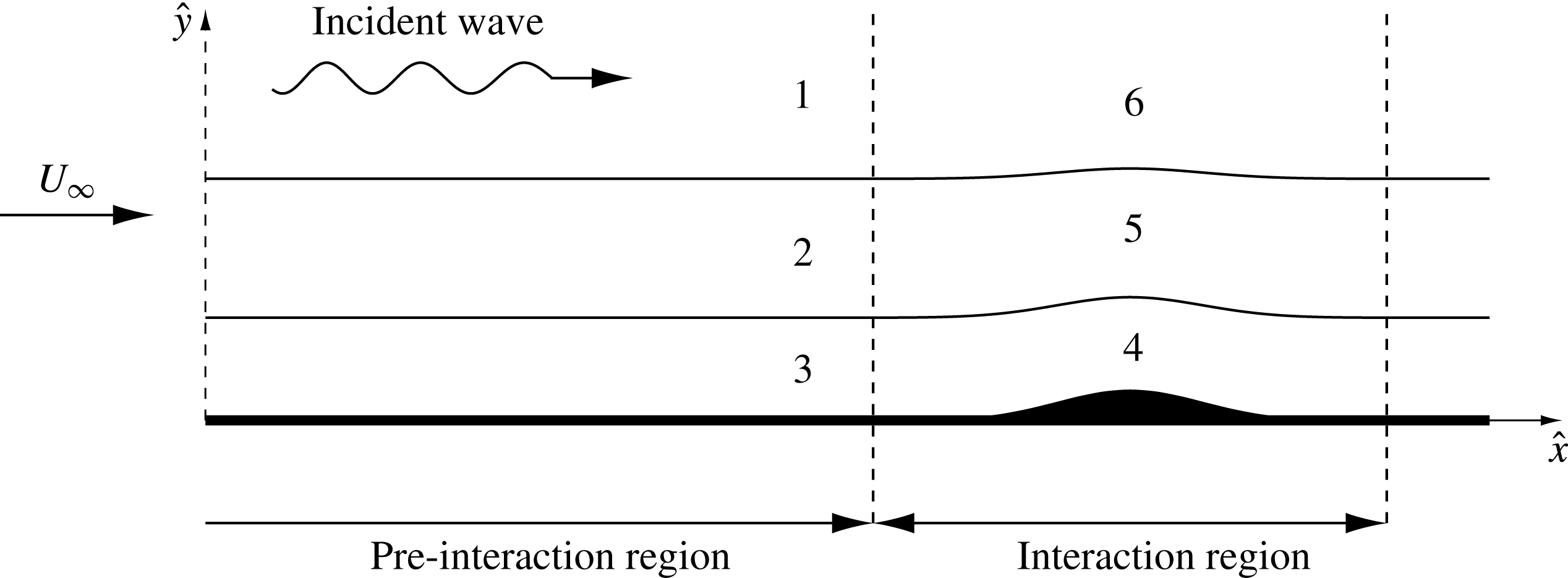
Figure 1. Illustration of the flow structure for the acoustic wave receptivity.
Let
![]() $U_{\infty }$
be the free-stream velocity and
$U_{\infty }$
be the free-stream velocity and
![]() $L$
the distance from the leading edge to the roughness. The values of the pressure, density and viscosity coefficient in the free stream are denoted by
$L$
the distance from the leading edge to the roughness. The values of the pressure, density and viscosity coefficient in the free stream are denoted by
![]() $p_{\infty }$
,
$p_{\infty }$
,
![]() ${\it\rho}_{\infty }$
and
${\it\rho}_{\infty }$
and
![]() ${\it\mu}_{\infty }$
, respectively. The Reynolds number is defined as
${\it\mu}_{\infty }$
, respectively. The Reynolds number is defined as
and is assumed to be large.
To perform the asymptotic analysis of the Navier–Stokes equations at large values of
![]() $\mathit{Re}$
, one needs to identify the resonance frequency
$\mathit{Re}$
, one needs to identify the resonance frequency
![]() ${\it\omega}$
of the acoustic wave and the characteristic length
${\it\omega}$
of the acoustic wave and the characteristic length
![]() $\ell$
of the wall roughness. As has already been mentioned, in subsonic flow
$\ell$
of the wall roughness. As has already been mentioned, in subsonic flow
To deduce the corresponding estimates for the transonic flow, one can proceed as follows. It is known that, in subsonic flow, the frequency and the wavelength of the neural Tollmien–Schlichting wave depend on the Mach number
![]() $M_{\infty }$
as follows:
$M_{\infty }$
as follows:
Keeping this in mind, Timoshin (Reference Timoshin1990) assumed that
![]() $M_{\infty }-1$
becomes progressively smaller and analysed the equations in the three tiers of the triple-deck model. He found that the triple-deck equations remain unchanged for all
$M_{\infty }-1$
becomes progressively smaller and analysed the equations in the three tiers of the triple-deck model. He found that the triple-deck equations remain unchanged for all
![]() $1-M_{\infty }^{2}\gg \mathit{Re}^{-1/9}$
. However, when
$1-M_{\infty }^{2}\gg \mathit{Re}^{-1/9}$
. However, when
![]() $1-M_{\infty }^{2}$
becomes a quantity of order
$1-M_{\infty }^{2}$
becomes a quantity of order
![]() $O(\mathit{Re}^{-1/9})$
, the flow in the upper deck can no longer be described by the Laplace equation. It has to be replaced by the transonic small-perturbation equation.
$O(\mathit{Re}^{-1/9})$
, the flow in the upper deck can no longer be described by the Laplace equation. It has to be replaced by the transonic small-perturbation equation.
Consequently, we shall assume that the free-stream Mach number
![]() $M_{\infty }$
is such that (see Timoshin Reference Timoshin1990; Bowles & Smith Reference Bowles and Smith1993)
$M_{\infty }$
is such that (see Timoshin Reference Timoshin1990; Bowles & Smith Reference Bowles and Smith1993)
where
![]() $Q_{\infty }$
is assumed to be an order-one quantity. It is referred to as the Kármán–Guderley parameter. Substitution of (2.5) into (2.4) shows that in the transonic flow the resonance conditions are achieved when
$Q_{\infty }$
is assumed to be an order-one quantity. It is referred to as the Kármán–Guderley parameter. Substitution of (2.5) into (2.4) shows that in the transonic flow the resonance conditions are achieved when
3. Flow ahead of the wall roughness
Here we shall consider the steady boundary layer that forms on the plate surface, and the perturbations produced in this flow by a weak acoustic wave travelling along the plate.
3.1. Steady compressible boundary-layer flow
The solution of the Navier–Stokes equations (2.1) for the steady flow in the boundary layer is represented in the form of the following asymptotic expansions:
Here the dimensionless coordinates
![]() $(\breve{x},\bar{Y})$
are introduced through the scalings
$(\breve{x},\bar{Y})$
are introduced through the scalings
Substitution of (3.1) and (3.2) into the Navier–Stokes equations (2.1) leads to the classical boundary-layer equations for compressible flow:
At the outer edge of the boundary layer, the conditions for matching of
![]() $U_{0}$
and
$U_{0}$
and
![]() $H_{0}$
with their values in the unperturbed flow outside the boundary layer are
$H_{0}$
with their values in the unperturbed flow outside the boundary layer are
In addition, the solution has to satisfy the no-slip conditions on the surface of the plate:
These have to be supplemented with an appropriate thermal condition. Here it will be assumed that the plate is thermally isolated, in which case
This boundary-value problem (3.3)–(3.6) admits a self-similar solution. However, for the receptivity analysis, we do not need to know the precise form of this solution. We only need to know that the solution is smooth near the position of roughness (
![]() $\breve{x}=1$
), and may be represented by the Taylor expansions
$\breve{x}=1$
), and may be represented by the Taylor expansions
 $$\begin{eqnarray}\displaystyle \left.\begin{array}{@{}c@{}}\displaystyle U_{0}(\breve{x},\bar{Y})=U_{00}(\bar{Y})+(\breve{x}-1)U_{01}(\bar{Y})+\cdots \,,\\ \displaystyle R_{0}(\breve{x},\bar{Y})=R_{00}(\bar{Y})+(\breve{x}-1)R_{01}(\bar{Y})+\cdots \,,\\ \displaystyle H_{0}(\breve{x},\bar{Y})=H_{00}(\bar{Y})+(\breve{x}-1)H_{01}(\bar{Y})+\cdots \,,\\ \displaystyle {\it\mu}_{0}(\breve{x},\bar{Y})={\it\mu}_{00}(\bar{Y})+(\breve{x}-1){\it\mu}_{01}(\bar{Y})+\cdots \,,\end{array}\!\!\right\} & & \displaystyle\end{eqnarray}$$
where
![]() $U_{00}(\bar{Y})$
,
$U_{00}(\bar{Y})$
,
![]() $R_{00}(\bar{Y})$
,
$R_{00}(\bar{Y})$
,
![]() $H_{00}(\bar{Y})$
and
$H_{00}(\bar{Y})$
and
![]() ${\it\mu}_{00}(\bar{Y})$
are such that
${\it\mu}_{00}(\bar{Y})$
are such that
 $$\begin{eqnarray}\left.\begin{array}{@{}c@{}}\displaystyle U_{00}(\bar{Y})={\it\tau}\bar{Y}+O(\bar{Y}^{4}),\\ \displaystyle R_{00}(\bar{Y})={\it\rho}_{w}+O(\bar{Y}^{2}),\\ \displaystyle H_{00}(\bar{Y})=h_{w}+O(\bar{Y}^{2}),\\ \displaystyle {\it\mu}_{00}(\bar{Y})={\it\mu}_{w}+O(\bar{Y}^{2}),\end{array}\!\!\right\}\quad \text{as }\bar{Y}\rightarrow 0,\end{eqnarray}$$
where
![]() ${\it\tau}$
denotes the skin friction, and
${\it\tau}$
denotes the skin friction, and
![]() $h_{w}$
,
$h_{w}$
,
![]() ${\it\mu}_{w}$
and
${\it\mu}_{w}$
and
![]() ${\it\rho}_{w}$
are the enthalpy, viscosity and density on the surface of the plate, respectively. All these quantities are constants.
${\it\rho}_{w}$
are the enthalpy, viscosity and density on the surface of the plate, respectively. All these quantities are constants.
3.2. Perturbations caused by acoustic noise
We start our analysis with region 1 situated outside the boundary layer (see figure 1). We shall assume that the acoustic noise is weak, and seek the corresponding solution of the Navier–Stokes equations (2.1) in the form
Substitution of (3.9) and (3.10) into the Navier–Stokes equation (2.1) leads to the linearised Euler equations:
By eliminating
![]() $u_{1}$
and
$u_{1}$
and
![]() ${\it\rho}_{1}$
, one can reduce the set of equations (3.11) to the following equation for the pressure perturbations
${\it\rho}_{1}$
, one can reduce the set of equations (3.11) to the following equation for the pressure perturbations
![]() $p_{1}$
:
$p_{1}$
:
It admits a travelling-wave solution
where
![]() $\bar{{\it\alpha}}$
is the amplitude of the acoustic wave,
$\bar{{\it\alpha}}$
is the amplitude of the acoustic wave,
![]() $\tilde{{\it\omega}}$
is the frequency and
$\tilde{{\it\omega}}$
is the frequency and
![]() $\bar{k}=-\tilde{{\it\omega}}M_{\infty }/(M_{\infty }+1)$
is the wavenumber.
$\bar{k}=-\tilde{{\it\omega}}M_{\infty }/(M_{\infty }+1)$
is the wavenumber.
3.3. Main part of the boundary layer
The steady solution in the boundary layer is represented by the asymptotic expansions (3.1). Now we shall add the perturbations caused by the acoustic wave:
Substituting (3.14) into (2.1) and working with the leading-order terms, we find that
The solution (3.16) does not satisfy the no-slip condition, which means that we also need to consider the Stokes layer closer to the plate surface.
3.4. Stokes layer
As the pressure perturbations (3.13) penetrate the boundary layer, they cause the Stokes layer to form near the surface. The thickness of this layer is easily estimated by comparing the instantaneous acceleration term with the viscous forces in the longitudinal momentum equation (2.1a ):
Taking into account that
![]() $\hat{{\it\rho}}\sim {\it\rho}_{\infty }$
,
$\hat{{\it\rho}}\sim {\it\rho}_{\infty }$
,
![]() $\hat{{\it\mu}}\sim {\it\mu}_{\infty }$
and the characteristic time is defined by (3.10b
), one can easily deduce from (3.17) that the thickness of the Stokes layer is
$\hat{{\it\mu}}\sim {\it\mu}_{\infty }$
and the characteristic time is defined by (3.10b
), one can easily deduce from (3.17) that the thickness of the Stokes layer is
![]() ${\hat{y}}\sim L\mathit{Re}^{-11/18}$
.
${\hat{y}}\sim L\mathit{Re}^{-11/18}$
.
The solution in the Stokes layer is sought in the form
 $$\begin{eqnarray}\left.\begin{array}{@{}c@{}}\displaystyle \hat{u} =U_{\infty }\mathit{Re}^{-1/9}u_{3}(\tilde{t},\bar{x},\bar{y})+\cdots \,,\\ \displaystyle \hat{v}=U_{\infty }\mathit{Re}^{-1/2}v_{3}(\tilde{t},\bar{x},\bar{y})+\cdots \,,\\ \displaystyle \hat{p}=p_{\infty }+{\it\rho}_{\infty }U_{\infty }^{2}\mathit{Re}^{-1/9}p_{3}(\tilde{t},\bar{x},\bar{y})+\cdots \,,\\ \displaystyle \hat{{\it\rho}}={\it\rho}_{\infty }[{\it\rho}_{w}+\mathit{Re}^{-1/9}{\it\rho}_{3}(\tilde{t},\bar{x},\bar{y})]+\cdots \,,\\ \displaystyle {\hat{h}}=U_{\infty }^{2}[h_{w}+\mathit{Re}^{-1/9}h_{3}(\tilde{t},\bar{x},\bar{y})]+\cdots \,,\\ \displaystyle \hat{{\it\mu}}={\it\mu}_{\infty }[{\it\mu}_{w}+\mathit{Re}^{-1/9}{\it\mu}_{3}(\tilde{t},\bar{x},\bar{y})]+\cdots \,,\end{array}\!\!\right\}\end{eqnarray}$$
where
![]() $\bar{y}$
is defined by the equation
$\bar{y}$
is defined by the equation
Substituting (3.18) into the Navier–Stokes equations (2.1) and working with leading-order terms, we find that the flow in the Stokes layer is described by the equations
It follows from (3.20b
) and (3.15b
) that the pressure does not change across the main part of the boundary layer, and it also remains unchanged across the Stokes layer. This means that
![]() $p_{3}$
is given by (3.13). With known
$p_{3}$
is given by (3.13). With known
![]() $p_{3}$
, the
$p_{3}$
, the
![]() $x$
momentum equation (3.20a
) separates from the rest of the equations in (3.20). It has to be solved with the no-slip condition on the surface of the plate and the matching condition with the solution in region
$x$
momentum equation (3.20a
) separates from the rest of the equations in (3.20). It has to be solved with the no-slip condition on the surface of the plate and the matching condition with the solution in region
![]() $2$
:
$2$
:
where
4. Flow in the interaction region
As was stated in the introduction, for effective generation of the Tollmien–Schlichting waves, the Stokes layer has to come into interaction with the wall roughness (see figure 2). To satisfy the resonance conditions, we shall assume that the longitudinal size of the roughness is estimated as
i.e. is comparable with the wavelength of the Tollmien–Schlichting wave. Keeping this in mind, we shall express the roughness shape by the equation
The triple-deck region that forms in the vicinity of the roughness is composed of three tiers: the viscous sublayer of thickness
![]() ${\hat{y}}\sim L\mathit{Re}^{-11/18}$
, the main part of the boundary layer with thickness
${\hat{y}}\sim L\mathit{Re}^{-11/18}$
, the main part of the boundary layer with thickness
![]() ${\hat{y}}\sim L\mathit{Re}^{-1/2}$
, and the potential flow region that lies outside the boundary layer; the thickness of the upper tier is estimated as
${\hat{y}}\sim L\mathit{Re}^{-1/2}$
, and the potential flow region that lies outside the boundary layer; the thickness of the upper tier is estimated as
![]() ${\hat{y}}\sim L\mathit{Re}^{-5/18}$
. Of course, all three layers have the same longitudinal extent given by (4.1). Correspondingly, an order-one longitudinal coordinate for the triple-deck region,
${\hat{y}}\sim L\mathit{Re}^{-5/18}$
. Of course, all three layers have the same longitudinal extent given by (4.1). Correspondingly, an order-one longitudinal coordinate for the triple-deck region,
![]() $\tilde{x}$
, is introduced as
$\tilde{x}$
, is introduced as
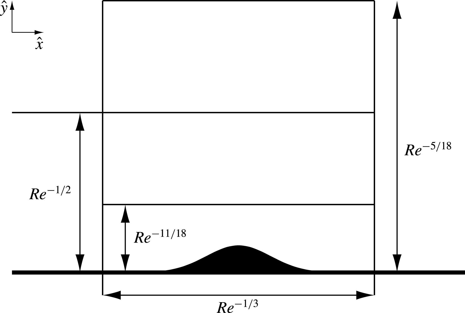
Figure 2. Triple-deck structure in transonic flow.
Before analysing the flow behaviour in the three tiers, we shall make the following observation. The size of the roughness is much smaller than the wavelength of the acoustic wave. Indeed, comparing (4.3) with (3.10a ), we can see that
Substituting (4.4) into (3.13) and setting
![]() $\mathit{Re}\rightarrow \infty$
with
$\mathit{Re}\rightarrow \infty$
with
![]() $\tilde{x}=O(1)$
, we find that, in the interaction region, the acoustic pressure perturbations may be expressed by the equation
$\tilde{x}=O(1)$
, we find that, in the interaction region, the acoustic pressure perturbations may be expressed by the equation
4.1. Lower deck
We start the analysis of the flow in the interaction region with the viscous near-wall layer, shown as region 4 in figure 1. The characteristic thickness of region 4 is the same as that of the Stokes layer (region 3). Keeping in mind that the solution in the Stokes layer is represented by asymptotic expansions (3.18), we seek the solution of the Navier–Stokes equations in region 4 in the form
 $$\begin{eqnarray}\left.\begin{array}{@{}c@{}}\displaystyle \hat{u} =U_{\infty }\mathit{Re}^{-1/9}u_{4}(\tilde{t},\tilde{x},\bar{y})+\cdots \,,\quad \hat{v}=U_{\infty }\mathit{Re}^{-7/18}v_{4}(\tilde{t},\tilde{x},\bar{y})+\cdots \,,\\ \displaystyle \hat{p}=p_{\infty }+{\it\rho}_{\infty }U_{\infty }^{2}\{\mathit{Re}^{-1/9}\bar{{\it\alpha}}\sin (\tilde{{\it\omega}}\tilde{t})+\mathit{Re}^{-2/9}[p_{4}(\tilde{t},\tilde{x},\bar{y})+\bar{{\it\alpha}}\bar{k}\,\tilde{x}\cos (\tilde{{\it\omega}}\tilde{t})]\}+\cdots \,,\\ \displaystyle \hat{{\it\rho}}={\it\rho}_{\infty }{\it\rho}_{w}+\cdots \,,\quad \hat{{\it\mu}}={\it\mu}_{\infty }{\it\mu}_{w}+\cdots \,,\quad {\hat{h}}=h_{\infty }h_{w}+\cdots \,,\end{array}\!\!\right\}\end{eqnarray}$$
with independent variables
![]() $\tilde{t}$
,
$\tilde{t}$
,
![]() $\tilde{x}$
and
$\tilde{x}$
and
![]() ${\tilde{y}}$
defined by
${\tilde{y}}$
defined by
Substitution of (4.6) and (4.7) into the Navier–Stokes equations (2.1) shows that pressure
![]() $p_{4}$
does not change across region 4, and the momentum (2.1a
) and continuity (2.1d
) equations assume the form
$p_{4}$
does not change across region 4, and the momentum (2.1a
) and continuity (2.1d
) equations assume the form
Equations (4.8) have to be solved with the no-slip conditions on the surface of the roughness,
and match with the solution (3.22) in the Stokes layer (region 3),
4.2. Middle deck
The flow in the middle deck (region 5 in figure 1) displays its usual behaviour. Owing to higher fluid velocity, this region is less sensitive to the pressure perturbation than the viscous sublayer. As a consequence, the middle deck does not contribute to the displacement effect of the boundary layer. Instead, it simply ‘transmits’ the deformations of the streamlines, produced in the viscous sublayer, to the upper deck. The solution in region 5 is constructed in the same way as was done for the corresponding subsonic flow (see Ruban Reference Ruban1984). We found that
For future use we need to mention that matching of (4.10a
) with the asymptotic expansion for
![]() $\hat{u}$
in (4.6) shows that the solution of equations (4.8) should satisfy the following boundary condition at the outer edge of the viscous sublayer layer (region 4):
$\hat{u}$
in (4.6) shows that the solution of equations (4.8) should satisfy the following boundary condition at the outer edge of the viscous sublayer layer (region 4):
We also need to perform the matching with the solution in the upper tier (region 6 in figure 1). Setting
![]() $\bar{Y}\rightarrow \infty$
in (4.10b
) and taking into account that
$\bar{Y}\rightarrow \infty$
in (4.10b
) and taking into account that
![]() $U_{00}(\infty )=1$
, we find that at the ‘bottom’ of region 6
$U_{00}(\infty )=1$
, we find that at the ‘bottom’ of region 6
4.3. Upper deck
Guided by (4.12) we represent the pressure in region 6 in the form of the asymptotic expansion
with the independent variables scaled as
The equation for the pressure perturbation function
![]() $p_{6}$
was deduced by Timoshin (Reference Timoshin1990). It has the form
$p_{6}$
was deduced by Timoshin (Reference Timoshin1990). It has the form
where
![]() $Q_{\infty }$
is defined by (2.5). Note that, in contrast to what happens in subsonic and supersonic flows, equation (4.15) retains the time derivative and is hyperbolic if
$Q_{\infty }$
is defined by (2.5). Note that, in contrast to what happens in subsonic and supersonic flows, equation (4.15) retains the time derivative and is hyperbolic if
![]() $Q_{\infty }>0$
, and elliptic otherwise.
$Q_{\infty }>0$
, and elliptic otherwise.
Equation (4.15) requires two boundary conditions. The first is the matching condition with the solution (4.12) in the middle tier. When written for the pressure perturbation function
![]() $p_{6}$
it has the form
$p_{6}$
it has the form
The second condition depends on the perturbation mode considered. If it is ‘subsonic’, then we will use the attenuation condition
If the flow regime is ‘supersonic’, then (4.16b ) will be substituted by a causality rule.
4.4. Viscous–inviscid interaction problem
When dealing with the interaction region, one has to solve equations (4.8) in the viscous sublayer simultaneously with (4.15) in the upper deck. The solution to equations (4.8) has to be found subject to the boundary conditions (4.9) and (4.11), while (4.15) has to be solved with the boundary condition (4.16) or its ‘supersonic’ counterpart. Considered together, these equations and boundary conditions constitute the viscous–inviscid interaction problem. To reduce the number of parameters involved, we shall perform the following affine transformation of the variables in the viscous sublayer:
 $$\begin{eqnarray}\displaystyle \left.\begin{array}{@{}c@{}}\displaystyle \tilde{t}=({\it\rho}_{w}{\it\mu}_{w}^{-5}{\it\tau}^{-14})^{1/9}t,\quad \tilde{x}=({\it\rho}_{w}^{-3}{\it\mu}_{w}^{-3}{\it\tau}^{-12})^{1/9}x,\\ \displaystyle \bar{y}=({\it\rho}_{w}^{-4}{\it\mu}_{w}^{2}{\it\tau}^{-7})^{1/9}[y+g(x)],\quad p_{4}=({\it\rho}_{w}{\it\mu}_{w}^{4}{\it\tau}^{4})^{1/9}p,\\ \displaystyle u_{4}=({\it\rho}_{w}^{-4}{\it\mu}_{w}^{2}{\it\tau}^{2})^{1/9}u,\quad v_{4}=({\it\rho}_{w}^{-5}{\it\mu}_{w}^{7}{\it\tau}^{7})^{1/9}\left[v+u\,\frac{\text{d}g}{\text{d}x}\right],\\ \displaystyle A_{\ast }=({\it\rho}_{w}^{-4}{\it\mu}_{w}^{2}{\it\tau}^{-7})^{1/9}[A-g(x)],\quad \bar{G}=({\it\rho}_{w}^{-4}{\it\mu}_{w}^{2}{\it\tau}^{-7})^{1/9}g(x).\end{array}\!\!\right\} & & \displaystyle\end{eqnarray}$$
Notice that, in addition to affine transformations, the above equations also include (in square brackets) the Prandtl transposition theorem.
The frequency and amplitude of the acoustic perturbation are scaled as
Correspondingly, for the upper deck we introduce the following transformations:
Finally, the Kármán–Guderley parameter is transformed as
As a result the lower-deck equations (4.8) assume the form
The upper-deck equation (4.15) is now written as
and the boundary conditions (4.16) assume the form
The statement that the pressure at the ‘bottom’ of region 6 coincides with the pressure in region 4,
closes the viscous–inviscid interaction problem.
5. Linear receptivity
Here we shall assume that the amplitude of the acoustic wave,
![]() ${\it\alpha}$
, is small, and the wall roughness is ‘shallow’, namely, we shall write the roughness equation in the form
${\it\alpha}$
, is small, and the wall roughness is ‘shallow’, namely, we shall write the roughness equation in the form
and apply to the interaction problem (4.21)–(4.25) the limit procedure
The asymptotic solution in the lower deck is sought in the form
represents the perturbations produced by the Stokes layer. The third term,
![]() $hu_{r}(x,y)$
, stands for the steady perturbations produced by the wall roughness. Finally, the fourth term,
$hu_{r}(x,y)$
, stands for the steady perturbations produced by the wall roughness. Finally, the fourth term,
![]() ${\it\alpha}hu^{\prime }(t,x,y)$
, represents the perturbations produced in the boundary layer due to the interaction of the Stokes layer with the steady flow field around the roughness.
${\it\alpha}hu^{\prime }(t,x,y)$
, represents the perturbations produced in the boundary layer due to the interaction of the Stokes layer with the steady flow field around the roughness.
Corresponding to (5.3), the solution in the upper deck is represented as
We start with the analysis of steady perturbations produced by the roughness.
5.1. Steady problem
Substituting (5.3) into (4.21) and (4.22), and working with
![]() $O(h)$
terms, we find that, in the viscous sublayer, the steady perturbations are described by the equations
$O(h)$
terms, we find that, in the viscous sublayer, the steady perturbations are described by the equations
Similarly, substitution of (5.5) into (4.23) and (4.20) results in
The solution of the problem (5.6)–(5.8) may be constructed in the same way as was done with the problem (4.14) and (4.15) in Ruban et al. (Reference Ruban, Bernots and Pryce2013). The main difference is that now (5.8a
) changes its type from elliptic in subsonic flow (
![]() $K_{\infty }<0$
) to hyperbolic in supersonic flow (
$K_{\infty }<0$
) to hyperbolic in supersonic flow (
![]() $K_{\infty }>0$
). In the latter case, the condition (5.8c
) has to be relaxed and substituted by the ‘causality condition’, according to which the perturbations produced by the roughness can only propagate downstream. As in Ruban et al. (Reference Ruban, Bernots and Pryce2013) we apply the Fourier transform to equation (5.8a
). With the Fourier transform of
$K_{\infty }>0$
). In the latter case, the condition (5.8c
) has to be relaxed and substituted by the ‘causality condition’, according to which the perturbations produced by the roughness can only propagate downstream. As in Ruban et al. (Reference Ruban, Bernots and Pryce2013) we apply the Fourier transform to equation (5.8a
). With the Fourier transform of
![]() $P_{r}(x,Y)$
defined as
$P_{r}(x,Y)$
defined as
we have
The solution to (5.10) and (5.11) satisfying the disturbance attenuation condition for
![]() $K_{\infty }<0$
, and the causality condition for
$K_{\infty }<0$
, and the causality condition for
![]() $K_{\infty }>0$
, has the form
$K_{\infty }>0$
, has the form
where
The solution of the boundary-value problem (5.6) and (5.7) for the viscous sublayer can now be found in the usual way (see e.g. Ruban et al. Reference Ruban, Bernots and Pryce2013). We have
where
![]() $z=(\text{i}k)^{1/3}y$
,
$z=(\text{i}k)^{1/3}y$
,
![]() $\bar{F}$
is the Fourier transform of the roughness shape function
$\bar{F}$
is the Fourier transform of the roughness shape function
![]() $F(x)$
, and
$F(x)$
, and
5.2. Unsteady problem
When dealing with the
![]() $O({\it\alpha}h)$
terms in (5.3) and (5.5), we have to solve the following equations in the viscous sublayer:
$O({\it\alpha}h)$
terms in (5.3) and (5.5), we have to solve the following equations in the viscous sublayer:
 $$\begin{eqnarray}\left.\begin{array}{@{}c@{}}\displaystyle \frac{\partial u^{\prime }}{\partial t}+y\frac{\partial u^{\prime }}{\partial x}+v^{\prime }+U_{s}\frac{\partial u_{r}}{\partial x}+v_{r}\frac{\partial U_{s}}{\partial y}=-\frac{\partial p^{\prime }}{\partial x}+\frac{\partial ^{2}u^{\prime }}{\partial y^{2}},\\ \displaystyle \frac{\partial u^{\prime }}{\partial x}+\frac{\partial v^{\prime }}{\partial y}=0.\end{array}\!\!\right\}\end{eqnarray}$$
The boundary conditions for (5.16) are
 $$\begin{eqnarray}\left.\begin{array}{@{}c@{}}\displaystyle u^{\prime }=v^{\prime }=0\quad \text{at }y=0,\\ \displaystyle u^{\prime }=A^{\prime }\quad \text{as }y\rightarrow \infty ,\\ \displaystyle u^{\prime }=0\quad \text{as }x\rightarrow -\infty .\end{array}\!\!\right\}\end{eqnarray}$$
In the upper deck the pressure perturbations are described by the equation
This has to be solved with the boundary conditions
 $$\begin{eqnarray}\left.\begin{array}{@{}c@{}}\displaystyle \frac{\partial P^{\prime }}{\partial Y}=\frac{\partial ^{2}A^{\prime }}{\partial x^{2}}\quad \text{at }Y=0,\\ \displaystyle P^{\prime }\rightarrow 0\quad \text{as }Y\rightarrow \infty .\end{array}\!\!\right\}\end{eqnarray}$$
The solution of the boundary-value problem (5.16)–(5.19) is sought in the time-periodic form:
where
![]() $\text{c.c.}$
denotes the complex conjugate, and
$\text{c.c.}$
denotes the complex conjugate, and
Substitution of (5.20) and (5.21) into (5.16) and (5.17) turns the boundary-value problem for the viscous sublayer into
 $$\begin{eqnarray}\left.\begin{array}{@{}c@{}}\displaystyle \text{i}{\it\omega}\tilde{u} +y\frac{\partial \tilde{u} }{\partial x}+\tilde{v}+\tilde{U} _{s}\frac{\partial u_{r}}{\partial x}+v_{r}\frac{\partial \tilde{U} _{s}}{\partial y}=-\frac{\partial \tilde{p}}{\partial x}+\frac{\partial ^{2}\tilde{u} }{\partial y^{2}},\\ \displaystyle \frac{\partial \tilde{u} }{\partial x}+\frac{\partial \tilde{v}}{\partial y}=0,\\ \displaystyle \tilde{u} =\tilde{v}=0\quad \text{at }y=0,\\ \displaystyle \tilde{u} =\tilde{A}\quad \text{as }y\rightarrow \infty ,\\ \tilde{u} =0\quad \text{as }x\rightarrow -\infty .\end{array}\!\!\right\}\end{eqnarray}$$
Similarly, the upper-deck boundary-value problem (5.18) and (5.19) takes the form
Applying the Fourier transform to (5.23a , b ), we have
 $$\begin{eqnarray}\left.\begin{array}{@{}c@{}}\displaystyle \frac{\text{d}^{2}\check{P}}{\text{d}Y^{2}}+(2{\it\omega}k+k^{2}K_{\infty })\check{P}=0,\\ \displaystyle \frac{\text{d}\check{P}}{\text{d}Y}=-k^{2}{\check{A}}\quad \text{at }Y=0.\end{array}\!\!\right\}\end{eqnarray}$$
Here
![]() $\check{P}$
is the Fourier transform of
$\check{P}$
is the Fourier transform of
![]() $\tilde{P}$
, and
$\tilde{P}$
, and
![]() ${\check{A}}$
is the Fourier transform of
${\check{A}}$
is the Fourier transform of
![]() $\tilde{A}$
. The solution to (5.24) satisfying the attenuation/causality conditions at large
$\tilde{A}$
. The solution to (5.24) satisfying the attenuation/causality conditions at large
![]() $Y$
is written as
$Y$
is written as
Here
![]() ${\it\sigma}$
is calculated for subsonic flow (
${\it\sigma}$
is calculated for subsonic flow (
![]() $K_{\infty }<0$
) as
$K_{\infty }<0$
) as
 $$\begin{eqnarray}{\it\sigma}=\left\{\begin{array}{@{}ll@{}}-\sqrt{2{\it\omega}k-k^{2}|K_{\infty }|}\quad & \displaystyle \text{for }k\in \left[0,\frac{2{\it\omega}}{|K_{\infty }|}\right],\\ \text{i}\sqrt{-2{\it\omega}k+k^{2}|K_{\infty }|}\quad & \displaystyle \text{for }k\in (-\infty ,0)\cup \left(\frac{2{\it\omega}}{|K_{\infty }|},\infty \right),\end{array}\right.\end{eqnarray}$$
and for the supersonic flow (
![]() $K_{\infty }>0$
) as
$K_{\infty }>0$
) as
 $$\begin{eqnarray}{\it\sigma}=\left\{\begin{array}{@{}ll@{}}\sqrt{-2{\it\omega}|k|+k^{2}K_{\infty }}\quad & \displaystyle \text{for }k\in \left(-\infty ,-\frac{2{\it\omega}}{|K_{\infty }|}\right),\\ \text{i}\sqrt{2{\it\omega}|k|-k^{2}K_{\infty }}\quad & \displaystyle \text{for }k\in \left[-\frac{2{\it\omega}}{|K_{\infty }|},0\right],\\ -\sqrt{2{\it\omega}k+k^{2}K_{\infty }}\quad & \displaystyle \text{for }k\in (0,\infty ).\end{array}\right.\end{eqnarray}$$
Setting
![]() $Y=0$
in (5.25) gives the Fourier transform of the pressure in the viscous sublayer:
$Y=0$
in (5.25) gives the Fourier transform of the pressure in the viscous sublayer:
The boundary-value problem (5.22) for the viscous sublayer is written in terms of the Fourier transforms as
This equation has to be solved with the boundary conditions
Equations (5.14) suggest that the solution of the boundary-value problem (5.30) and (5.31) may be represented as
Introducing a new independent variable
where
![]() ${\it\zeta}_{0}=\text{i}{\it\omega}/(\text{i}k)^{2/3}$
, it is easily shown that
${\it\zeta}_{0}=\text{i}{\it\omega}/(\text{i}k)^{2/3}$
, it is easily shown that
![]() $\text{d}\bar{\bar{u}}/\text{d}{\it\zeta}$
satisfies the inhomogeneous Airy equation:
$\text{d}\bar{\bar{u}}/\text{d}{\it\zeta}$
satisfies the inhomogeneous Airy equation:
with
This should be solved subject to the following boundary conditions:
The general solution of (5.34) is a composition of two complementary solutions of the Airy equation and a particular integral:
Here we choose
![]() ${\it\varphi}({\it\zeta})$
to be the solution to the following boundary-value problem:
${\it\varphi}({\it\zeta})$
to be the solution to the following boundary-value problem:
To avoid exponential growth of
![]() $\text{d}\bar{\bar{u}}/\text{d}{\it\zeta}$
as
$\text{d}\bar{\bar{u}}/\text{d}{\it\zeta}$
as
![]() ${\it\zeta}\rightarrow \infty$
, we set
${\it\zeta}\rightarrow \infty$
, we set
![]() $C_{2}=0$
in (5.37). Thus, we have
$C_{2}=0$
in (5.37). Thus, we have
Then, applying boundary conditions (5.36), we obtain two equations for the constant
![]() $C_{1}$
and the displacement function
$C_{1}$
and the displacement function
![]() $\bar{\bar{A}}$
:
$\bar{\bar{A}}$
:
Eliminating
![]() $C_{1}$
from (5.40), we find that
$C_{1}$
from (5.40), we find that
 $$\begin{eqnarray}\bar{\bar{A}}=\frac{\displaystyle \text{Ai}^{\prime }({\it\zeta}_{0})\int _{{\it\zeta}_{0}}^{\infty }{\it\varphi}(s)\,\text{d}s}{\displaystyle \text{Ai}^{\prime }({\it\zeta}_{0})-\text{i}(\text{i}k)^{1/3}k^{2}{\it\sigma}^{-1}\int _{{\it\zeta}_{0}}^{\infty }\text{Ai}(s)\,\text{d}s}.\end{eqnarray}$$
Finally, we substitute (5.41) into (5.31b ) and then into (5.28). We find that the Fourier transform of the pressure is given by
 $$\begin{eqnarray}\check{p}=\frac{\displaystyle \text{i}k^{2}\text{Ai}^{\prime }({\it\zeta}_{0})\bar{F}(k)\int _{{\it\zeta}_{0}}^{\infty }{\it\varphi}(s)\,\text{d}s}{\displaystyle {\it\sigma}\text{Ai}^{\prime }({\it\zeta}_{0})-\text{i}(\text{i}k)^{1/3}k^{2}\int _{{\it\zeta}_{0}}^{\infty }\text{Ai}(s)\,\text{d}s}.\end{eqnarray}$$
To return to physical variables, one needs to apply the inverse Fourier transform to (5.42):
 $$\begin{eqnarray}P(t,x)=\frac{\text{e}^{\text{i}{\it\omega}t}}{2{\rm\pi}}\int _{-\infty }^{\infty }\frac{\text{i}k^{2}\text{Ai}^{\prime }({\it\zeta}_{0})\displaystyle \int _{{\it\zeta}_{0}}^{\infty }{\it\varphi}(s)\,\text{d}s}{{\it\sigma}\text{Ai}^{\prime }({\it\zeta}_{0})-\text{i}(\text{i}k)^{1/3}k^{2}\displaystyle \int _{{\it\zeta}_{0}}^{\infty }\text{Ai}(s)\,\text{d}s}\bar{F}(k)\text{e}^{\text{i}kx}\,\text{d}k.\end{eqnarray}$$
Here the integration is performed along the real axis in the
![]() $k$
-plane. For our purposes, it is convenient to take the analytic extension of the integrand into the complex
$k$
-plane. For our purposes, it is convenient to take the analytic extension of the integrand into the complex
![]() $k$
-plane, and deform the contour of integration. When performing this task, one needs to know the singularities of the integrand. Setting the denominator in (5.43) to zero results in the following dispersion relation:
$k$
-plane, and deform the contour of integration. When performing this task, one needs to know the singularities of the integrand. Setting the denominator in (5.43) to zero results in the following dispersion relation:
with
![]() ${\it\sigma}$
and
${\it\sigma}$
and
![]() ${\it\zeta}_{0}$
defined as in (5.26), (5.27) and (5.33).
${\it\zeta}_{0}$
defined as in (5.26), (5.27) and (5.33).
When solving (5.44) we will assume that the frequency,
![]() ${\it\omega}$
, is real and positive. Our task will be to find the wavenumber,
${\it\omega}$
, is real and positive. Our task will be to find the wavenumber,
![]() $k$
, which in the general case is complex and is a function of
$k$
, which in the general case is complex and is a function of
![]() ${\it\omega}$
and
${\it\omega}$
and
![]() $K_{\infty }$
. We expect the Tollmien–Schlichting waves to propagate downstream, which happens when the real part of the wavenumber is negative. Also, when solving the dispersion equation (5.44), it should be remembered that the real part of
$K_{\infty }$
. We expect the Tollmien–Schlichting waves to propagate downstream, which happens when the real part of the wavenumber is negative. Also, when solving the dispersion equation (5.44), it should be remembered that the real part of
![]() $\sqrt{2{\it\omega}k+k^{2}K_{\infty }}$
has been assumed positive in (5.26) and (5.27). We start the calculations by assuming that
$\sqrt{2{\it\omega}k+k^{2}K_{\infty }}$
has been assumed positive in (5.26) and (5.27). We start the calculations by assuming that
![]() ${\it\omega}\rightarrow 0$
and
${\it\omega}\rightarrow 0$
and
![]() ${\it\zeta}_{0}$
is finite, which consequently leads to the limit
${\it\zeta}_{0}$
is finite, which consequently leads to the limit
![]() $k\rightarrow 0$
. In addition, it can be deduced from (5.33) that
$k\rightarrow 0$
. In addition, it can be deduced from (5.33) that
![]() ${\it\omega}$
is an
${\it\omega}$
is an
![]() $O(k^{2/3})$
quantity and thus
$O(k^{2/3})$
quantity and thus
![]() ${\it\sigma}=O(k)$
. Taking these into account, we can see that the dispersion equation (5.44) reduces to
${\it\sigma}=O(k)$
. Taking these into account, we can see that the dispersion equation (5.44) reduces to
The above equation has an infinite number of roots, all of them lying on the negative real semi-axis in the
![]() ${\it\zeta}_{0}$
-plane. This suggests that the dispersion equation (5.44) has an infinite number of roots. In figure 3 we show five of these. Each root was calculated by using the corresponding root of (5.45) as an initial guess for a small value of
${\it\zeta}_{0}$
-plane. This suggests that the dispersion equation (5.44) has an infinite number of roots. In figure 3 we show five of these. Each root was calculated by using the corresponding root of (5.45) as an initial guess for a small value of
![]() ${\it\omega}$
. Then the dispersion relation (5.44) was solved using Newton iterations, where the frequency was kept fixed until the iteration process converged and the corresponding value of
${\it\omega}$
. Then the dispersion relation (5.44) was solved using Newton iterations, where the frequency was kept fixed until the iteration process converged and the corresponding value of
![]() ${\it\zeta}_{0}$
was found. The process was then repeated for a new, larger value of
${\it\zeta}_{0}$
was found. The process was then repeated for a new, larger value of
![]() ${\it\omega}$
. The results of the calculations are shown in figure 3. We see that in the
${\it\omega}$
. The results of the calculations are shown in figure 3. We see that in the
![]() ${\it\zeta}_{0}$
-plane, all the roots originate from the points defined by (5.45), and all of them, except the first one, tend to finite points in the
${\it\zeta}_{0}$
-plane, all the roots originate from the points defined by (5.45), and all of them, except the first one, tend to finite points in the
![]() ${\it\zeta}_{0}$
-plane as
${\it\zeta}_{0}$
-plane as
![]() ${\it\omega}\rightarrow \infty$
. In this limit the dispersion equation (5.44) reduces to
${\it\omega}\rightarrow \infty$
. In this limit the dispersion equation (5.44) reduces to
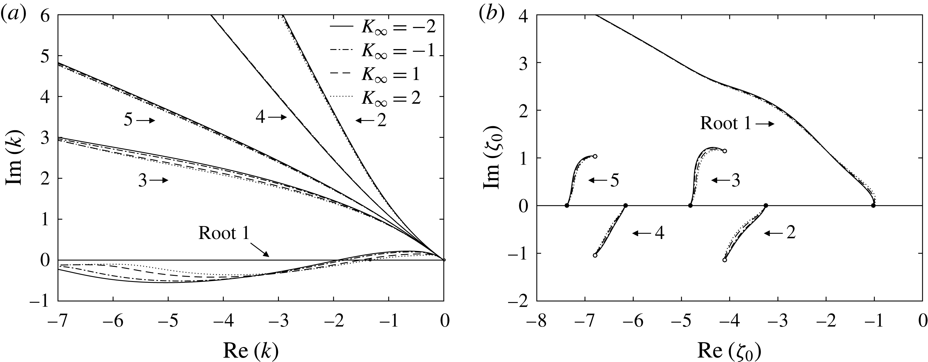
Figure 3. The first five roots of the dispersion equation in the (a)
![]() $k$
-plane and (b)
$k$
-plane and (b)
![]() ${\it\zeta}_{0}$
-plane.
${\it\zeta}_{0}$
-plane.
Equation (5.46) has an infinite number of roots, which all come in complex conjugate pairs and lie in the left half of the
![]() ${\it\zeta}_{0}$
-plane. As far as the first root is concerned, its behaviour is different. For this root,
${\it\zeta}_{0}$
-plane. As far as the first root is concerned, its behaviour is different. For this root,
![]() ${\it\zeta}_{0}$
moves to infinity as
${\it\zeta}_{0}$
moves to infinity as
![]() ${\it\omega}\rightarrow \infty$
(see figure 3
b). This root also behaves differently in the
${\it\omega}\rightarrow \infty$
(see figure 3
b). This root also behaves differently in the
![]() $k$
-plane. While all the other roots remain in the second quadrant for all
$k$
-plane. While all the other roots remain in the second quadrant for all
![]() ${\it\omega}$
, representing the modes that decay downstream, the first root crosses the real axis at point
${\it\omega}$
, representing the modes that decay downstream, the first root crosses the real axis at point
![]() $k=k_{0}<0$
at a critical value
$k=k_{0}<0$
at a critical value
![]() ${\it\omega}_{0}$
of the frequency
${\it\omega}_{0}$
of the frequency
![]() ${\it\omega}$
. Both
${\it\omega}$
. Both
![]() $k_{0}$
and
$k_{0}$
and
![]() ${\it\omega}_{0}$
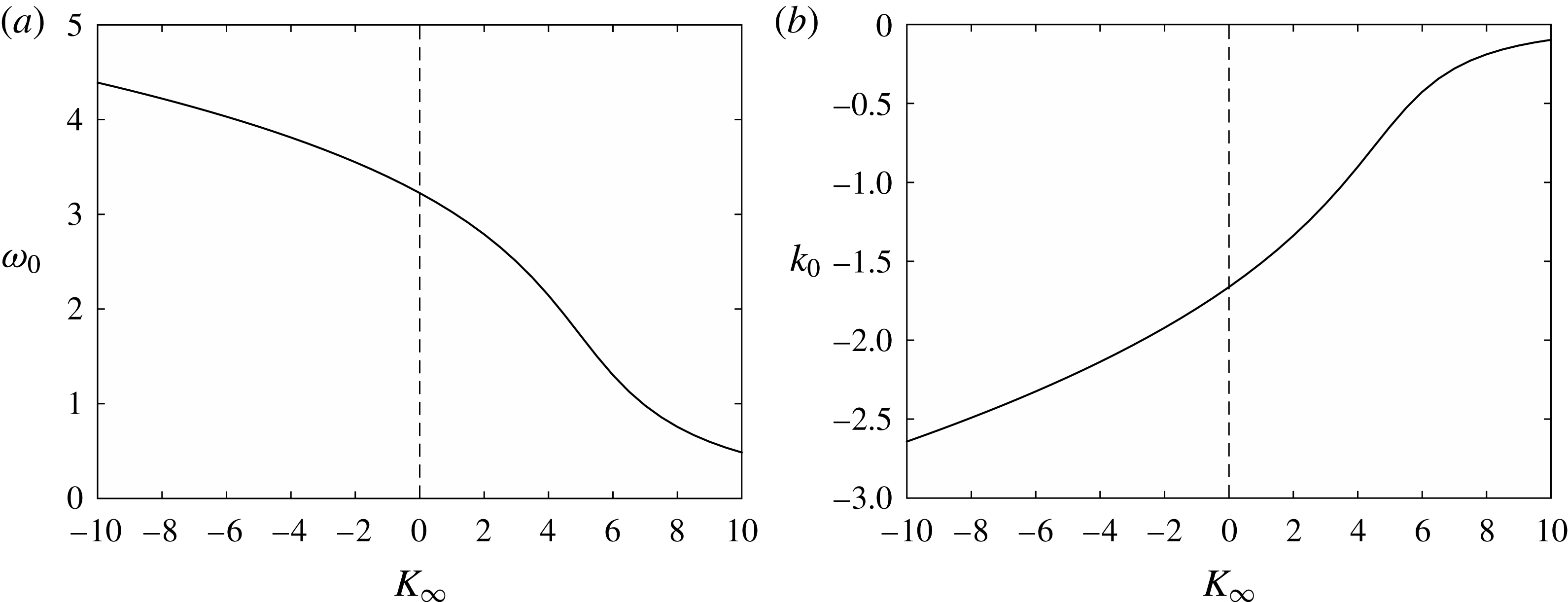
depend on the Kármán–Guderley parameter. This root represents the Tollmien–Schlichting wave, which appears to be neutral at
${\it\omega}_{0}$
depend on the Kármán–Guderley parameter. This root represents the Tollmien–Schlichting wave, which appears to be neutral at
![]() ${\it\omega}={\it\omega}_{0}$
. For all
${\it\omega}={\it\omega}_{0}$
. For all
![]() ${\it\omega}>{\it\omega}_{0}$
this root remains in the third quadrant, which signifies that the Tollmien–Schlichting wave is growing downstream. It is interesting to note that
${\it\omega}>{\it\omega}_{0}$
this root remains in the third quadrant, which signifies that the Tollmien–Schlichting wave is growing downstream. It is interesting to note that
![]() $|k_{0}|$
decreases as the Kármán–Guderley parameter
$|k_{0}|$
decreases as the Kármán–Guderley parameter
![]() $K_{\infty }$
increases (see Ryzhov Reference Ryzhov2012).
$K_{\infty }$
increases (see Ryzhov Reference Ryzhov2012).
A way to determine how
![]() $k_{0}$
depends on
$k_{0}$
depends on
![]() $K_{\infty }$
was suggested by Timoshin (Reference Timoshin1990). He noticed that, in the case of neutral perturbations, the transonic dispersion equation (5.44) can easily be reduced to the dispersion equation for incompressible flow:
$K_{\infty }$
was suggested by Timoshin (Reference Timoshin1990). He noticed that, in the case of neutral perturbations, the transonic dispersion equation (5.44) can easily be reduced to the dispersion equation for incompressible flow:
To perform this task, it is convenient to introduce the phase velocity
![]() $c_{0}={\it\omega}_{0}/k_{0}$
, and perform the affine transformations
$c_{0}={\it\omega}_{0}/k_{0}$
, and perform the affine transformations
where
![]() $c_{0}^{\ast }=-2.296$
,
$c_{0}^{\ast }=-2.296$
,
![]() $k_{0}^{\ast }=-1.00049$
is the neutral solution of (5.47). The transformations (5.48) turn (5.44) into
$k_{0}^{\ast }=-1.00049$
is the neutral solution of (5.47). The transformations (5.48) turn (5.44) into
Comparison of (5.47) with (5.49) leads to the following equation for constant
![]() $a$
:
$a$
:
This equation has only one real solution whose behaviour is shown in figure 4.

Figure 4. (a) Neutral frequency and (b) wavenumber as functions of the Kármán–Guderley parameter.
Let us now return to the integral (5.43). Our intention is to deform the integration path in the
![]() $k$
-plane. We shall distinguish between two cases: subsonic (
$k$
-plane. We shall distinguish between two cases: subsonic (
![]() $K_{\infty }<0$
) and supersonic (
$K_{\infty }<0$
) and supersonic (
![]() $K_{\infty }>0$
). In both cases we start by considering a value of the frequency that is smaller than the critical frequency. For such
$K_{\infty }>0$
). In both cases we start by considering a value of the frequency that is smaller than the critical frequency. For such
![]() ${\it\omega}$
, all the roots of (5.44) lie in the second quadrant of the complex
${\it\omega}$
, all the roots of (5.44) lie in the second quadrant of the complex
![]() $k$
-plane. We have to remember that, when introducing an analytical branch of the function
$k$
-plane. We have to remember that, when introducing an analytical branch of the function
![]() $(\text{i}k)^{1/3}$
, we had to make a branch cut along the positive imaginary axis in the
$(\text{i}k)^{1/3}$
, we had to make a branch cut along the positive imaginary axis in the
![]() $k$
-plane. Therefore, we have to split the integration interval in (5.43) into two parts, negative and positive real semi-axes.
$k$
-plane. Therefore, we have to split the integration interval in (5.43) into two parts, negative and positive real semi-axes.
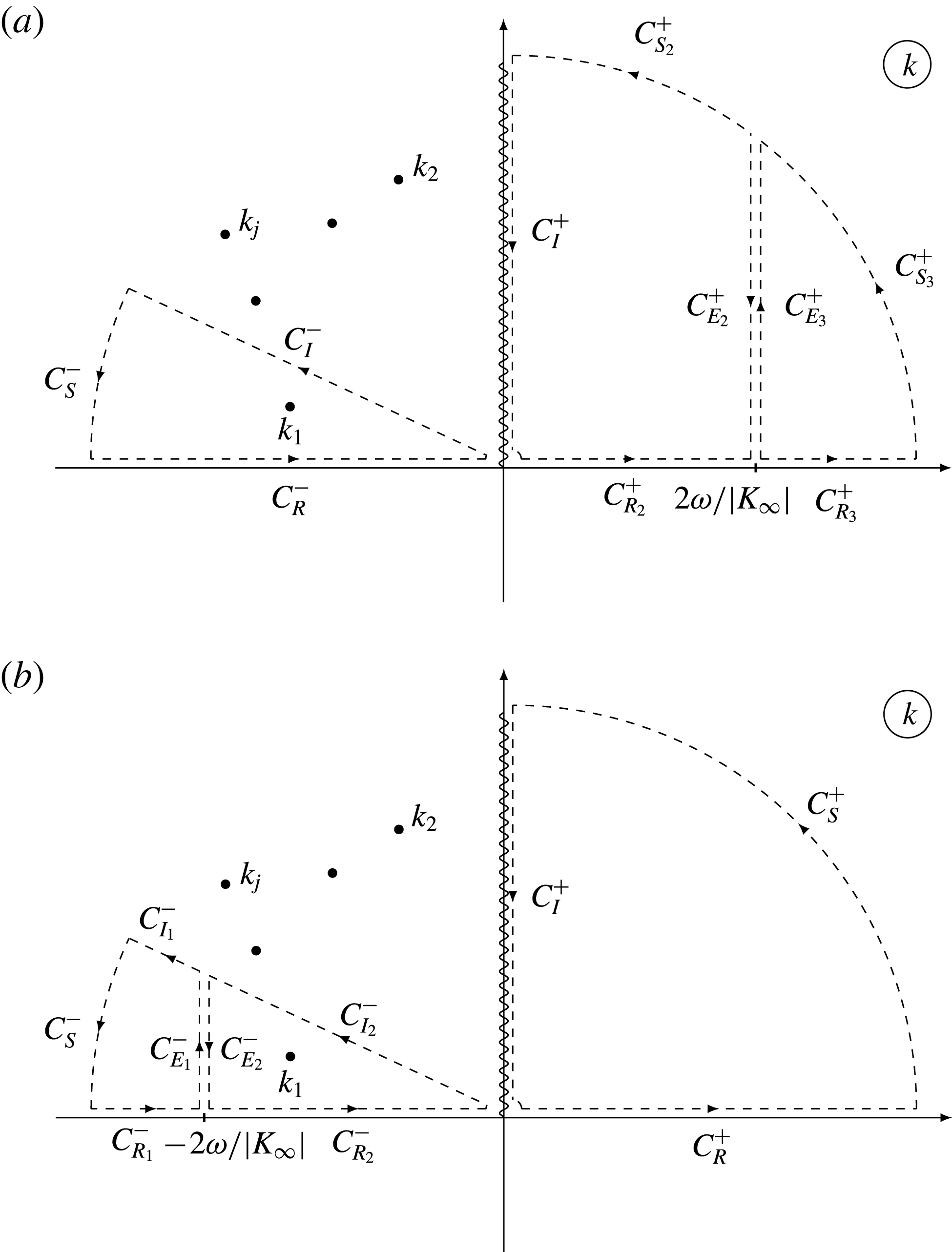
Figure 5. The contour of integration in the
![]() $k$
-plane for (a) negative and (b) positive values of the Kármán–Guderley parameter.
$k$
-plane for (a) negative and (b) positive values of the Kármán–Guderley parameter.
In the case of negative
![]() $K_{\infty }$
, we close the contour along the real negative semi-axis with an arc
$K_{\infty }$
, we close the contour along the real negative semi-axis with an arc
![]() $C_{S}^{-}$
of a large radius
$C_{S}^{-}$
of a large radius
![]() $R$
and a ray
$R$
and a ray
![]() $C_{I}^{-}$
originating at the coordinate origin (see figure 5
a). The angle between the negative real semi-axis and
$C_{I}^{-}$
originating at the coordinate origin (see figure 5
a). The angle between the negative real semi-axis and
![]() $C_{I}^{-}$
is chosen so that the closed contour encloses only one root
$C_{I}^{-}$
is chosen so that the closed contour encloses only one root
![]() $k_{1}$
. To calculate the integral along the real positive semi-axis, we introduce two closed contours (
$k_{1}$
. To calculate the integral along the real positive semi-axis, we introduce two closed contours (
![]() $C_{R_{2}}^{+},C_{E_{2}}^{+},C_{S_{2}}^{+},C_{I}^{+}$
) and (
$C_{R_{2}}^{+},C_{E_{2}}^{+},C_{S_{2}}^{+},C_{I}^{+}$
) and (
![]() $C_{R_{3}}^{+},C_{S_{3}}^{+},C_{E_{3}}^{+}$
) divided by the point
$C_{R_{3}}^{+},C_{S_{3}}^{+},C_{E_{3}}^{+}$
) divided by the point
![]() $k=2{\it\omega}/|K_{\infty }|$
on the real axis.
$k=2{\it\omega}/|K_{\infty }|$
on the real axis.
Using the residue theorem and setting
![]() $R\rightarrow \infty$
, we can then write (5.43) as
$R\rightarrow \infty$
, we can then write (5.43) as
 $$\begin{eqnarray}\displaystyle P(t,x) & = & \displaystyle -\frac{3\text{i}q_{1}k_{1}^{2}\text{Ai}^{\prime }({\it\zeta}_{0})\displaystyle \int _{{\it\zeta}_{0}}^{\infty }{\it\varphi}(s)\,\text{d}s\,\bar{F}(k_{1})\text{e}^{\text{i}({\it\omega}t+k_{1}x)}}{3\text{Ai}^{\prime }({\it\zeta}_{0})[K_{\infty }k_{1}+{\it\omega}]+q_{1}(\text{i}k_{1})^{1/3}\left[2\text{Ai}({\it\zeta}_{0}){\it\zeta}_{0}\left(q_{1}\displaystyle \frac{{\it\omega}}{k_{1}^{2}}+k_{1}\right)+7k_{1}I_{{\it\zeta}_{0}}\right]}\nonumber\\ \displaystyle & & \displaystyle -\,\frac{\text{e}^{\text{i}{\it\omega}t}}{2{\rm\pi}}\left[\int _{C_{I}^{-}}+\int _{C_{I}^{+}}\right],\end{eqnarray}$$
where
The first term in the above equation is the residue at point
![]() $k_{1}$
. Note that, using the Jordan lemma, we have disregarded the integrals along
$k_{1}$
. Note that, using the Jordan lemma, we have disregarded the integrals along
![]() $C_{S}^{-}$
,
$C_{S}^{-}$
,
![]() $C_{S_{2}}^{+}$
and
$C_{S_{2}}^{+}$
and
![]() $C_{S_{3}}^{+}$
. Further, using the Watson lemma, it may be shown (see Bernots Reference Bernots2014) that at large values of
$C_{S_{3}}^{+}$
. Further, using the Watson lemma, it may be shown (see Bernots Reference Bernots2014) that at large values of
![]() $x$
the contribution of the integrals along the rays
$x$
the contribution of the integrals along the rays
![]() $C_{I}^{-}$
and
$C_{I}^{-}$
and
![]() $C_{I}^{+}$
in (5.51) amounts to
$C_{I}^{+}$
in (5.51) amounts to
Thus we can conclude that at large values of
![]() $x$
and negative values of the Kármán–Guderley parameter,
$x$
and negative values of the Kármán–Guderley parameter,
where
![]() $\mathscr{K}({\it\omega},K_{\infty })$
is the receptivity coefficient. It is a function of the frequency
$\mathscr{K}({\it\omega},K_{\infty })$
is the receptivity coefficient. It is a function of the frequency
![]() ${\it\omega}$
and the Kármán–Guderley parameter
${\it\omega}$
and the Kármán–Guderley parameter
![]() $K_{\infty }$
. It is calculated as
$K_{\infty }$
. It is calculated as
 $$\begin{eqnarray}\mathscr{K}=-\frac{\displaystyle 3\text{i}q_{1}k_{1}^{2}\text{Ai}^{\prime }({\it\zeta}_{0})\int _{{\it\zeta}_{0}}^{\infty }{\it\varphi}(s)\,\text{d}s}{3\text{Ai}^{\prime }({\it\zeta}_{0})[K_{\infty }k_{1}+{\it\omega}]+q_{1}(\text{i}k_{1})^{1/3}\left[2\text{Ai}({\it\zeta}_{0}){\it\zeta}_{0}\left(q_{1}\displaystyle \frac{{\it\omega}}{k_{1}^{2}}+k_{1}\right)+7k_{1}I_{{\it\zeta}_{0}}\right]}.\end{eqnarray}$$
The above analysis can be repeated for positive
![]() $K_{\infty }$
, now deforming the contour of integration as shown in figure 5(b). Interestingly, the results of the analysis can be expressed again by (5.54) and (5.55). The first term on the right-hand side of (5.54) represents the Tollmien–Schlichting wave. Its amplitude is given by the product of the receptivity coefficient
$K_{\infty }$
, now deforming the contour of integration as shown in figure 5(b). Interestingly, the results of the analysis can be expressed again by (5.54) and (5.55). The first term on the right-hand side of (5.54) represents the Tollmien–Schlichting wave. Its amplitude is given by the product of the receptivity coefficient
![]() $\mathscr{K}$
and the Fourier transform of the roughness shape function
$\mathscr{K}$
and the Fourier transform of the roughness shape function
![]() $\bar{F}(k_{1})$
calculated at
$\bar{F}(k_{1})$
calculated at
![]() $k=k_{1}$
.
$k=k_{1}$
.
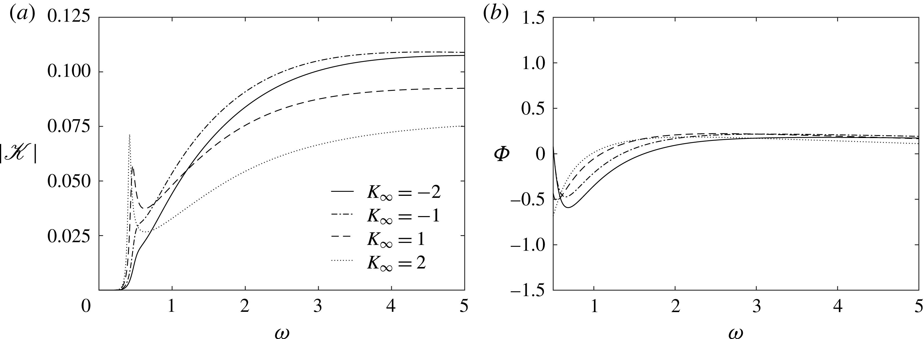
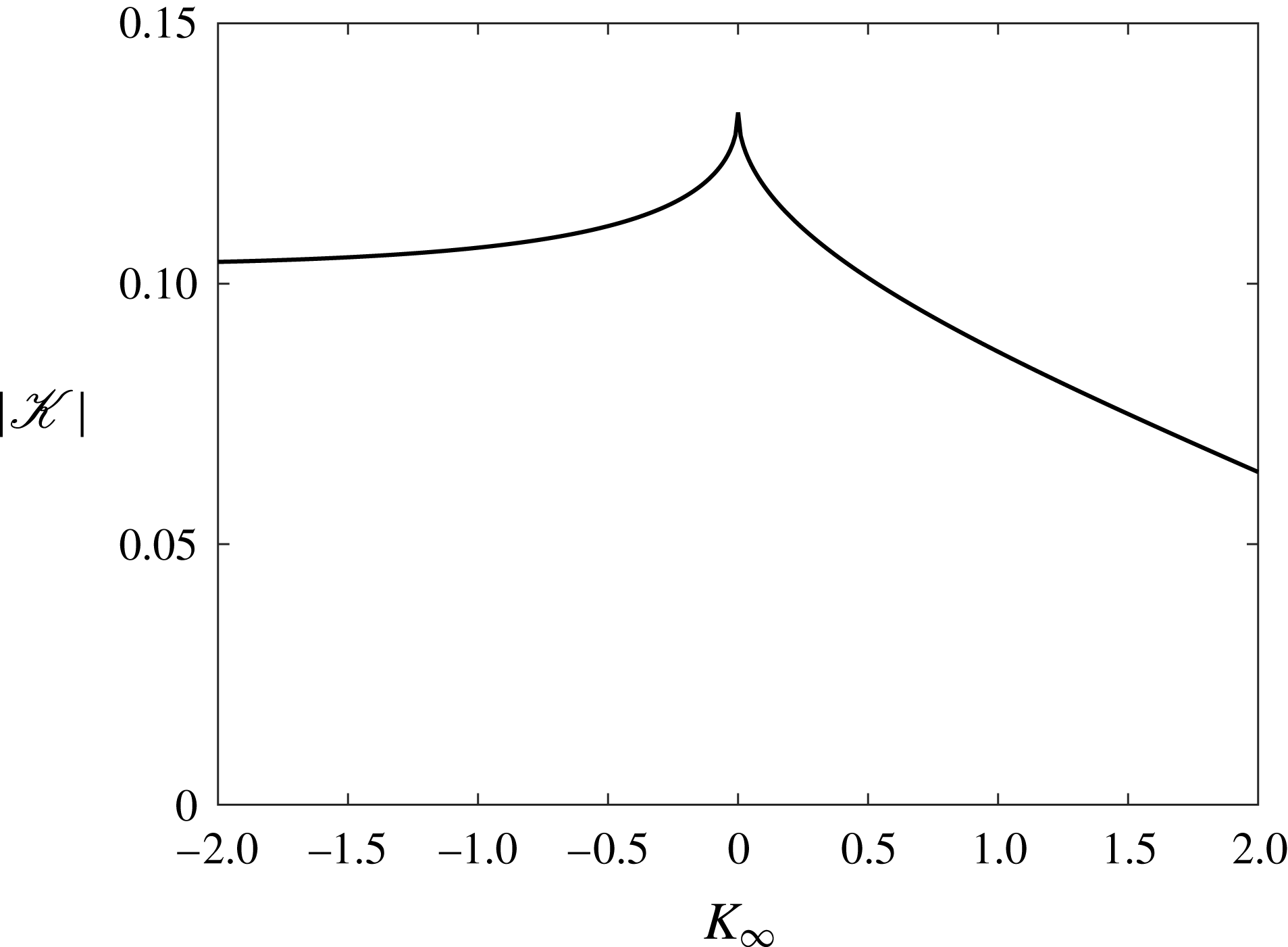
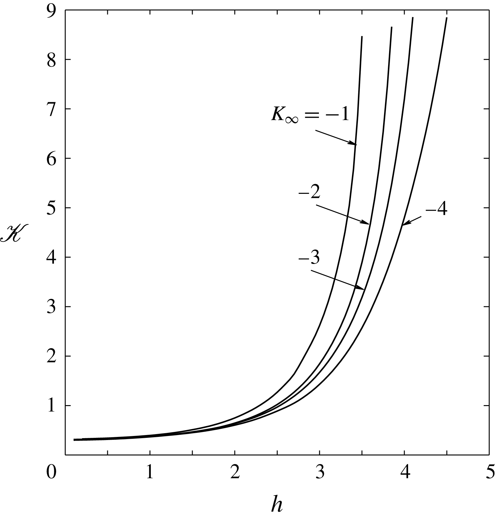
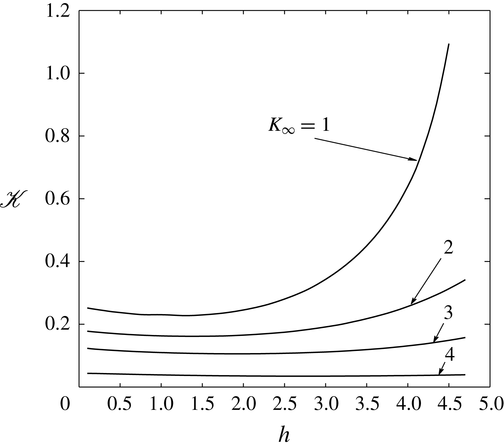
The results of the numerical calculation of the receptivity coefficient are shown in figures 6 and 7. It is interesting to note that
![]() $|\mathscr{K}|$
reaches its maximum when
$|\mathscr{K}|$
reaches its maximum when
![]() $K_{\infty }=0$
, i.e. the free-stream Mach number
$K_{\infty }=0$
, i.e. the free-stream Mach number
![]() $M_{\infty }$
is exactly one.
$M_{\infty }$
is exactly one.
6. Nonlinear receptivity problem
We shall now assume that the roughness height parameter
![]() $h$
is an order-one quantity. The amplitude
$h$
is an order-one quantity. The amplitude
![]() ${\it\alpha}$
of the acoustic wave will still be assumed small. In this case the solution of the viscous–inviscid interaction problem (4.21)–(4.25) can be represented in the form
${\it\alpha}$
of the acoustic wave will still be assumed small. In this case the solution of the viscous–inviscid interaction problem (4.21)–(4.25) can be represented in the form
 $$\begin{eqnarray}\left.\begin{array}{@{}c@{}}\displaystyle u(x,y,t)=u_{0}(x,y)+{\it\alpha}u_{1}(x,y,t)+\cdots \,,\\ \displaystyle v(x,y,t)=v_{0}(x,y)+{\it\alpha}v_{1}(x,y,t)+\cdots \,,\\ \displaystyle p(x,t)=p_{0}(x)+{\it\alpha}p_{1}(x,t)+\cdots \,,\\ \displaystyle A(x,t)=A_{0}(x)+{\it\alpha}A_{1}(x,t)+\cdots \,,\\ \displaystyle P(x,Y,t)=P_{0}(x,Y)+{\it\alpha}P_{1}(x,Y,t)+\cdots \,.\end{array}\!\!\right\}\end{eqnarray}$$

Figure 6. Receptivity coefficient modulus (a) and argument (b).

Figure 7. Dependence of the receptivity coefficient on
![]() $K_{\infty }$
for neutral
$K_{\infty }$
for neutral
![]() ${\it\omega}_{0}$
and
${\it\omega}_{0}$
and
![]() $k_{0}$
.
$k_{0}$
.
6.1. Nonlinear steady solution
Setting
![]() ${\it\alpha}=0$
in (4.21) and (4.22) gives the equations for the steady flow past the roughness in the lower deck:
${\it\alpha}=0$
in (4.21) and (4.22) gives the equations for the steady flow past the roughness in the lower deck:
Substitution of (6.1) and (5.1) into boundary condition (4.24a ) renders it in the form
If the flow is supersonic (
![]() $K_{\infty }>0$
), then the general solution to (6.4) is written as
$K_{\infty }>0$
), then the general solution to (6.4) is written as
with the two terms representing the perturbations that propagate downstream and upstream, respectively. The causality rule suggests that the second term should be disregarded. Taking this into account, and using boundary condition (6.5), one can find that at the ‘bottom’ of the upper deck the Ackeret formula holds:
In subsonic flow (
![]() $K_{\infty }<0$
) the solution of (6.4) satisfying boundary condition (6.5) and the condition of attenuation of the perturbations as
$K_{\infty }<0$
) the solution of (6.4) satisfying boundary condition (6.5) and the condition of attenuation of the perturbations as
![]() $Y\rightarrow \infty$
is expressed by the Hilbert integral of thin airfoil theory:
$Y\rightarrow \infty$
is expressed by the Hilbert integral of thin airfoil theory:
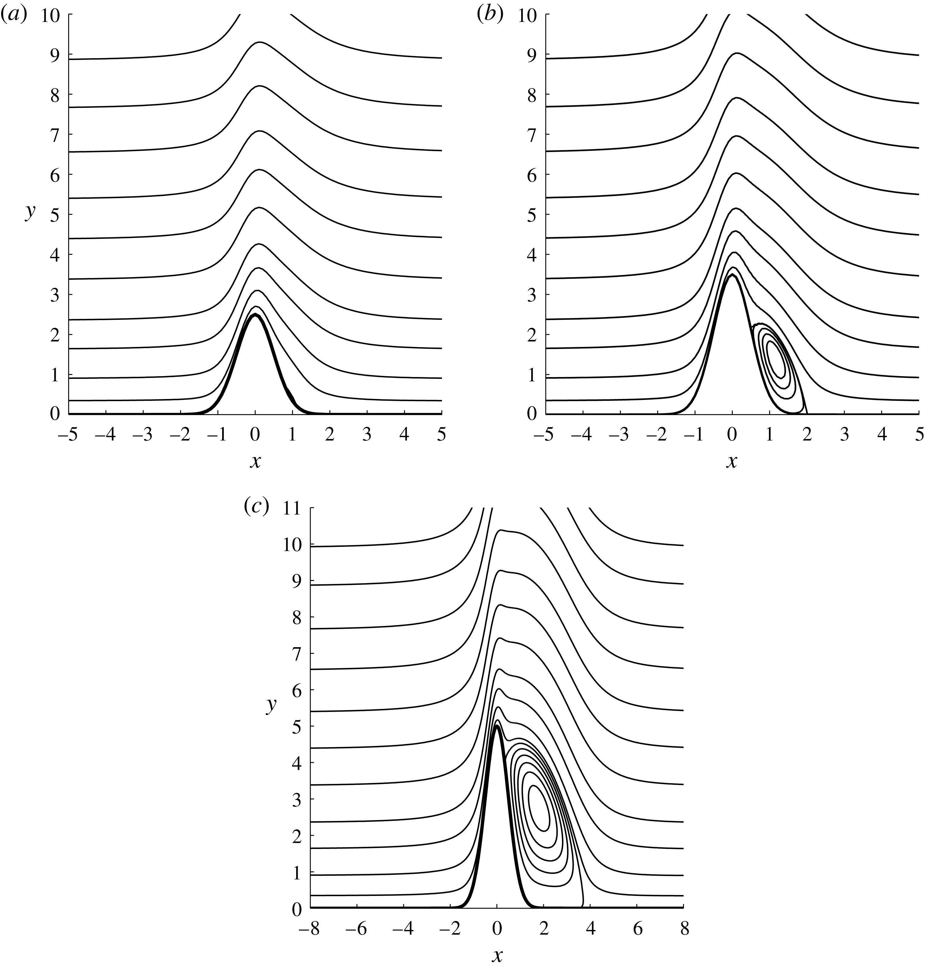
Figure 8. Streamlines for the steady flow,
![]() $K_{\infty }=-2$
: (a)
$K_{\infty }=-2$
: (a)
![]() $h=2.5$
; (b)
$h=2.5$
; (b)
![]() $h=3.5$
; (c)
$h=3.5$
; (c)
![]() $h=5.0$
.
$h=5.0$
.
To solve the steady viscous–inviscid interaction problem as formulated above, we used the numerical technique suggested by Kravtsova, Zametaev & Ruban (Reference Kravtsova, Zametaev and Ruban2005). We shall give here a short description of the method. For more details, the reader is referred to the original paper of Kravtsova et al. (Reference Kravtsova, Zametaev and Ruban2005). To perform the calculations, we introduce a discrete mesh
![]() $\{x_{i}\}$
, where
$\{x_{i}\}$
, where
![]() $i=1,\ldots ,N$
, and denote the vector composed of the values of
$i=1,\ldots ,N$
, and denote the vector composed of the values of
![]() $A_{0}$
at the mesh points by
$A_{0}$
at the mesh points by
![]() $\boldsymbol{A}$
. We also consider the vector
$\boldsymbol{A}$
. We also consider the vector
![]() $\boldsymbol{B}$
whose elements are the values of the pressure gradient
$\boldsymbol{B}$
whose elements are the values of the pressure gradient
![]() $\text{d}p/\text{d}x$
at the mesh points. Then, the finite-difference representation of the inviscid equations (6.7) and (6.8) can be expressed in the form
$\text{d}p/\text{d}x$
at the mesh points. Then, the finite-difference representation of the inviscid equations (6.7) and (6.8) can be expressed in the form
where
![]() $\unicode[STIX]{x1D647}$
is a linear operator. Also, given the displacement function
$\unicode[STIX]{x1D647}$
is a linear operator. Also, given the displacement function
![]() $\boldsymbol{A}$
, equations (6.2) and (6.3) allow us to calculate the velocity field
$\boldsymbol{A}$
, equations (6.2) and (6.3) allow us to calculate the velocity field
![]() $(u_{0},v_{0})$
in the viscous sublayer and the pressure gradient. The latter may be expressed in the form
$(u_{0},v_{0})$
in the viscous sublayer and the pressure gradient. The latter may be expressed in the form
where
![]() $\unicode[STIX]{x1D649}$
is a nonlinear operator. Our task is to find
$\unicode[STIX]{x1D649}$
is a nonlinear operator. Our task is to find
![]() $\boldsymbol{A}$
such that the pressure gradient (6.9) defined by the outer solution coincides with the pressure gradient (6.10) defined by the inner solution. Following the formalism of the Newtonian method, we start with an approximate distribution of the displacement function
$\boldsymbol{A}$
such that the pressure gradient (6.9) defined by the outer solution coincides with the pressure gradient (6.10) defined by the inner solution. Following the formalism of the Newtonian method, we start with an approximate distribution of the displacement function
![]() $\widetilde{\boldsymbol{A}}$
and introduce a correction,
$\widetilde{\boldsymbol{A}}$
and introduce a correction,
![]() ${\it\delta}\boldsymbol{A}$
. Then, assuming
${\it\delta}\boldsymbol{A}$
. Then, assuming
![]() ${\it\delta}\boldsymbol{A}$
to be small, equations (6.9) and (6.10) may be written as
${\it\delta}\boldsymbol{A}$
to be small, equations (6.9) and (6.10) may be written as
The requirement that the pressure gradient should be the same in the viscous sublayer and at the ‘bottom’ of the upper deck leads to the following equation for the correction
![]() ${\it\delta}\boldsymbol{A}$
:
${\it\delta}\boldsymbol{A}$
:
The most time-consuming part of the numerical procedure is the calculation of the elements of the matrices
![]() $\unicode[STIX]{x1D647}$
and
$\unicode[STIX]{x1D647}$
and
![]() $\unicode[STIX]{x1D649}$
. On each iteration, we first calculate the ‘viscous’ and ‘inviscid’ pressure gradients for a given
$\unicode[STIX]{x1D649}$
. On each iteration, we first calculate the ‘viscous’ and ‘inviscid’ pressure gradients for a given
![]() $\widetilde{\boldsymbol{A}}$
, and then repeat the calculations
$\widetilde{\boldsymbol{A}}$
, and then repeat the calculations
![]() $N$
times with the displacement function perturbed at a single point
$N$
times with the displacement function perturbed at a single point
![]() $x_{i}$
. Comparing the perturbed and unperturbed results allows us to determine the
$x_{i}$
. Comparing the perturbed and unperturbed results allows us to determine the
![]() $i$
th columns in matrices
$i$
th columns in matrices
![]() $\unicode[STIX]{x1D647}$
and
$\unicode[STIX]{x1D647}$
and
![]() $\unicode[STIX]{x1D649}$
.
$\unicode[STIX]{x1D649}$
.
Some of the results of the calculations are shown in figure 8 in the form of streamline patterns. Here we choose the Kármán–Guderley parameter to be
![]() $K_{\infty }=-2$
, and the shape of the roughness
$K_{\infty }=-2$
, and the shape of the roughness
![]() $F=\text{e}^{-2x^{2}}$
. In this case the separation region forms when the roughness height is
$F=\text{e}^{-2x^{2}}$
. In this case the separation region forms when the roughness height is
![]() $h=2.5$
, and it increases in size as
$h=2.5$
, and it increases in size as
![]() $h$
is growing.
$h$
is growing.
6.2. Unsteady problem formulation
The equations for the unsteady perturbations are obtained by substituting (6.1) into (4.21) and (4.22), and working with
![]() $O({\it\alpha})$
terms. We find that in the viscous sublayer the flow is described by the linear boundary-layer equations
$O({\it\alpha})$
terms. We find that in the viscous sublayer the flow is described by the linear boundary-layer equations
These have to be solved with the no-slip conditions of the surface of the roughness,
the condition of matching with the solution in the middle deck,
and the condition of matching with the solution upstream of the roughness,
 $$\begin{eqnarray}\displaystyle u_{1} & = & \displaystyle \frac{1}{{\it\omega}}\left\{\left[1-\text{e}^{-\sqrt{{\it\omega}/2}y}\cos \left(\sqrt{\frac{{\it\omega}}{2}}y\right)\right]\sin ({\it\omega}t)\right.\nonumber\\ \displaystyle & & \displaystyle +\,\text{e}^{-\sqrt{{\it\omega}/2}y}\sin \left.\left(\sqrt{\frac{{\it\omega}}{2}}y\right)\cos ({\it\omega}t)\right\}+\cdots \quad \text{as }x\rightarrow -\infty .\end{eqnarray}$$
In the upper tier we have to solve (5.18) subject to the boundary conditions (5.19). In the notation used here, these are written as
We shall seek the solution in the viscous sublayer in the form
 $$\begin{eqnarray}\left.\begin{array}{@{}c@{}}\displaystyle u_{1}=u_{11}\sin ({\it\omega}t)+u_{12}\cos ({\it\omega}t),\\ \displaystyle v_{1}=v_{11}\sin ({\it\omega}t)+v_{12}\cos ({\it\omega}t),\\ \displaystyle p_{1}=p_{11}\sin ({\it\omega}t)+p_{12}\cos ({\it\omega}t),\\ \displaystyle A_{1}=A_{11}\sin ({\it\omega}t)+A_{12}\cos ({\it\omega}t).\end{array}\!\!\right\}\end{eqnarray}$$
Substitution of (6.15) into (6.13) results in the following set of linear equations:
These have to be solved subject to the boundary conditions
6.3. Transonic interaction law for
 $K_{\infty }<0$
Now our task will be to express the solution of (6.14a ) for the upper deck in a form suitable for numerical analysis. We assume that the solution is periodic in time, namely,
Substitution of (6.18) into (6.14a ) yields
The above equation can be reduced to the Helmholtz equation
by means of the transformations
Similar to the pressure
![]() $P_{1}$
, we represent the displacement function
$P_{1}$
, we represent the displacement function
![]() $A_{1}$
in the time-periodic form
$A_{1}$
in the time-periodic form
and then the boundary condition (6.14b ) turns into
where
Let us introduce a point source in (6.20) centred at point
![]() $(x_{0},y_{10})$
:
$(x_{0},y_{10})$
:
where
![]() ${\it\delta}$
is the Dirac delta function. The two fundamental solutions of (6.25), which are functions of the distance
${\it\delta}$
is the Dirac delta function. The two fundamental solutions of (6.25), which are functions of the distance
![]() $r=\sqrt{(x-x_{0})^{2}+(y_{1}-y_{10})^{2}}$
from the source only, are
$r=\sqrt{(x-x_{0})^{2}+(y_{1}-y_{10})^{2}}$
from the source only, are
where
![]() $\text{H}_{0}^{(1)}$
and
$\text{H}_{0}^{(1)}$
and
![]() $\text{H}_{0}^{(2)}$
are Hankel functions. It is well known that (see e.g. Abramowitz & Stegun Reference Abramowitz and Stegun1965)
$\text{H}_{0}^{(2)}$
are Hankel functions. It is well known that (see e.g. Abramowitz & Stegun Reference Abramowitz and Stegun1965)
 $$\begin{eqnarray}\left.\begin{array}{@{}c@{}}\displaystyle \text{H}_{0}^{(1)}(z)=\sqrt{\frac{2}{{\rm\pi}z}}\text{e}^{\text{i}(z-{\rm\pi}/4)}+\cdots \,,\\ \displaystyle \text{H}_{0}^{(2)}(z)=\sqrt{\frac{2}{{\rm\pi}z}}\text{e}^{-\text{i}(z-{\rm\pi}/4)}+\cdots \end{array}\!\!\right\}\quad \text{as }z\rightarrow \infty .\end{eqnarray}$$
Substituting (6.27) into (6.26) and using
![]() $V_{1,2}$
instead of
$V_{1,2}$
instead of
![]() $p_{v}$
in (6.21), we find from (6.18) that, at large values of
$p_{v}$
in (6.21), we find from (6.18) that, at large values of
![]() $y_{1}$
,
$y_{1}$
,

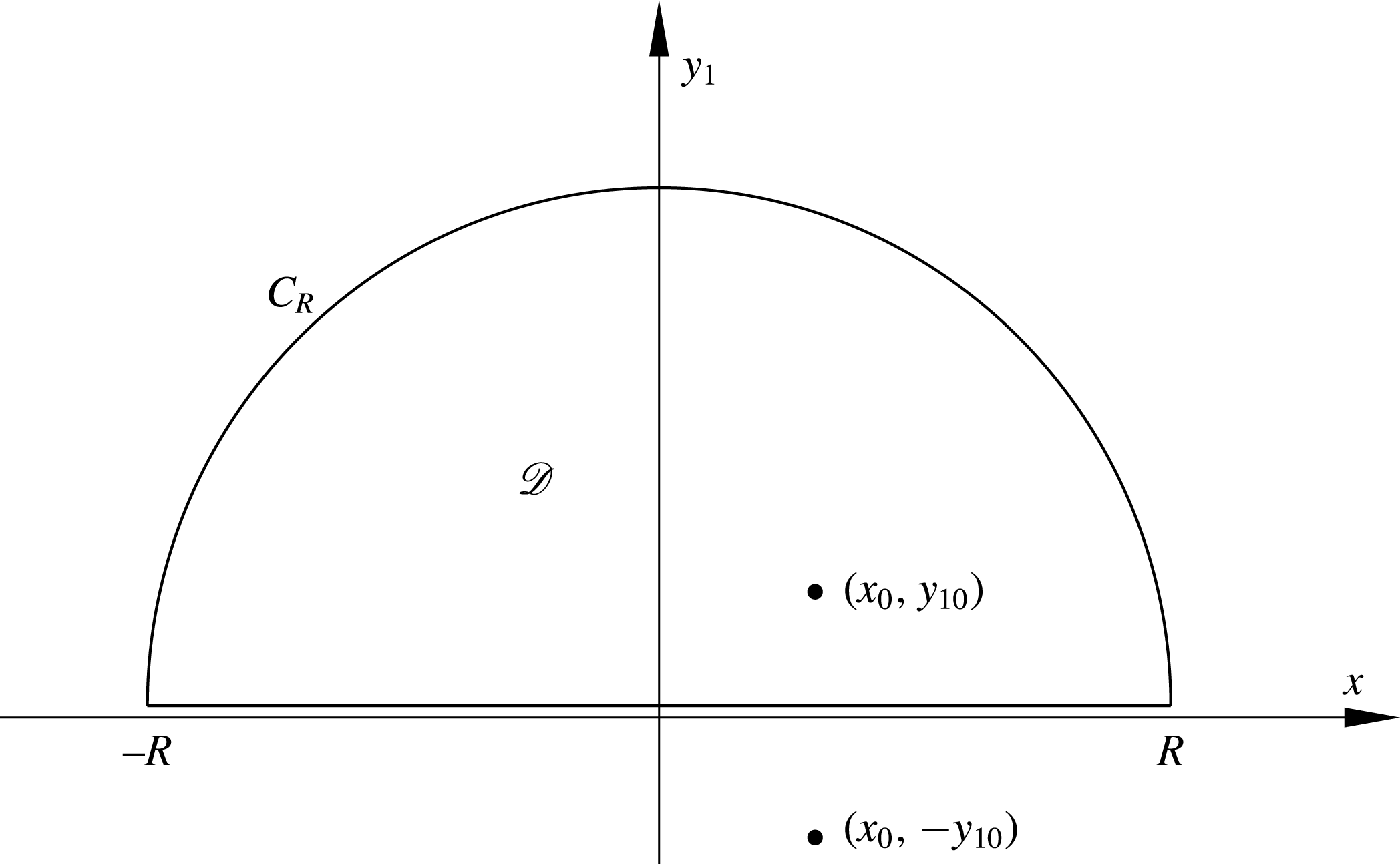
Figure 9. Region
![]() $\mathscr{D}$
used in equation (6.29).
$\mathscr{D}$
used in equation (6.29).
Let us consider region
![]() $\mathscr{D}$
inside a closed contour that is composed of a semicircle
$\mathscr{D}$
inside a closed contour that is composed of a semicircle
![]() $C_{R}$
of a large radius
$C_{R}$
of a large radius
![]() $R$
and a segment
$R$
and a segment
![]() $[-R,R]$
of the
$[-R,R]$
of the
![]() $x$
-axis (see figure 9). Green’s formula applied to this region is written as
$x$
-axis (see figure 9). Green’s formula applied to this region is written as
 $$\begin{eqnarray}\displaystyle \iint _{\mathscr{D}}(U{\rm\nabla}^{2}V-V{\rm\nabla}^{2}U)\,\text{d}x\,\text{d}y_{1} & = & \displaystyle \left.\int _{-R}^{R}\left(U\frac{\partial V}{\partial n}-V\frac{\partial U}{\partial n}\right)\right|_{y_{1}=0}\,\text{d}x\nonumber\\ \displaystyle & & \displaystyle +\,\int _{C_{R}}\left(U\frac{\partial V}{\partial n}-V\frac{\partial U}{\partial n}\right)\,\text{d}s,\end{eqnarray}$$
We choose
![]() $U$
in (6.29) to coincide with
$U$
in (6.29) to coincide with
![]() $p_{v}$
, and
$p_{v}$
, and
![]() $V$
to coincide with the second function in (6.26). Keeping in mind that
$V$
to coincide with the second function in (6.26). Keeping in mind that
![]() $V\sim 1/\sqrt{y_{1}}$
and
$V\sim 1/\sqrt{y_{1}}$
and
![]() $p_{v}$
has to satisfy the attenuation condition, we can disregard the second integral on the right-hand side of (6.29). It follows from (6.20) and (6.25) that, in region
$p_{v}$
has to satisfy the attenuation condition, we can disregard the second integral on the right-hand side of (6.29). It follows from (6.20) and (6.25) that, in region
![]() $\mathscr{D}$
,
$\mathscr{D}$
,
Using (6.30) in the integral on the left-hand side of (6.29), we have
Keeping in mind that
![]() $n$
is the external normal to region
$n$
is the external normal to region
![]() $\mathscr{D}$
, and using the boundary condition (6.23) for
$\mathscr{D}$
, and using the boundary condition (6.23) for
![]() $U$
, we have
$U$
, we have
which turns (6.31) into
Here the superscript
![]() $(+)$
in
$(+)$
in
![]() $V_{2}^{(+)}$
is used to indicate that
$V_{2}^{(+)}$
is used to indicate that
![]() $V_{2}^{(+)}$
is the solution of (6.25) with the source situated at point
$V_{2}^{(+)}$
is the solution of (6.25) with the source situated at point
![]() $(x_{0},y_{0})$
above the
$(x_{0},y_{0})$
above the
![]() $x$
-axis.
$x$
-axis.
Let us now reflect the source in the
![]() $x$
-axis (see figure 9), and write (6.25) in the form
$x$
-axis (see figure 9), and write (6.25) in the form
Our interest again is in the second of the solutions (6.26), which describes the perturbations radiated by the roughness. We shall write it as
where
![]() $r=\sqrt{(x-x_{0})^{2}+(y_{1}+y_{10})^{2}}$
. If we choose
$r=\sqrt{(x-x_{0})^{2}+(y_{1}+y_{10})^{2}}$
. If we choose
![]() $U=p_{v}$
and
$U=p_{v}$
and
![]() $V=V_{2}^{(-)}$
in Green’s formula (6.29), and take into account that now the source is situated outside region
$V=V_{2}^{(-)}$
in Green’s formula (6.29), and take into account that now the source is situated outside region
![]() $\mathscr{D}$
, then instead of (6.33) we will have
$\mathscr{D}$
, then instead of (6.33) we will have
It is easily seen that
which means that
![]() $p_{v}$
can be eliminated from the integral on the right-hand side of (6.33) by simply adding (6.36) to (6.33). This results in
$p_{v}$
can be eliminated from the integral on the right-hand side of (6.33) by simply adding (6.36) to (6.33). This results in
Making use of (6.24) and of the second of the solutions (6.26), we can write (6.38) in the form
It remains to return to (6.21), and we can conclude that the solution in the upper deck is written as
When performing the unsteady flow calculations, we used the above equation to form the matrix
![]() $\unicode[STIX]{x1D647}$
in (6.9). The rest of the numerical procedure is the same as in § 6.1. The results of the calculations are presented in figures 10 and 11. In figure 10 we show the pressure gradient distribution along the body surface for a particular value of the Kármán–Guderley parameter
$\unicode[STIX]{x1D647}$
in (6.9). The rest of the numerical procedure is the same as in § 6.1. The results of the calculations are presented in figures 10 and 11. In figure 10 we show the pressure gradient distribution along the body surface for a particular value of the Kármán–Guderley parameter
![]() $K_{\infty }=-1$
. According to the linear theory (see § 5), the neutral frequency for
$K_{\infty }=-1$
. According to the linear theory (see § 5), the neutral frequency for
![]() $K_{\infty }=-1$
is
$K_{\infty }=-1$
is
![]() ${\it\omega}_{0}=3.35$
(see figure 4
a). Figure 10 shows that the perturbations decay downstream of the roughness if
${\it\omega}_{0}=3.35$
(see figure 4
a). Figure 10 shows that the perturbations decay downstream of the roughness if
![]() ${\it\omega}<{\it\omega}_{0}$
, and start growing if
${\it\omega}<{\it\omega}_{0}$
, and start growing if
![]() ${\it\omega}>{\it\omega}_{0}$
.
${\it\omega}>{\it\omega}_{0}$
.
Figure 11 shows how the receptivity coefficient
![]() $\mathscr{K}$
depends on the roughness height
$\mathscr{K}$
depends on the roughness height
![]() $h$
. Here, for each value of the Kármán–Guderley parameter, we chose the frequency
$h$
. Here, for each value of the Kármán–Guderley parameter, we chose the frequency
![]() ${\it\omega}$
to coincide with the neutral frequency (see figure 4
a), and repeated the calculations for a sequence of values of
${\it\omega}$
to coincide with the neutral frequency (see figure 4
a), and repeated the calculations for a sequence of values of
![]() $h$
. We then determined the amplitude of the oscillations of the pressure gradient in the Tollmien–Schlichting wave downstream of the roughness. The receptivity coefficient is the ratio of this amplitude and the roughness height
$h$
. We then determined the amplitude of the oscillations of the pressure gradient in the Tollmien–Schlichting wave downstream of the roughness. The receptivity coefficient is the ratio of this amplitude and the roughness height
![]() $h$
. It is interesting to note that the receptivity coefficient starts to grow rapidly as soon as the separation region forms in the flow past the roughness (see figure 8).
$h$
. It is interesting to note that the receptivity coefficient starts to grow rapidly as soon as the separation region forms in the flow past the roughness (see figure 8).
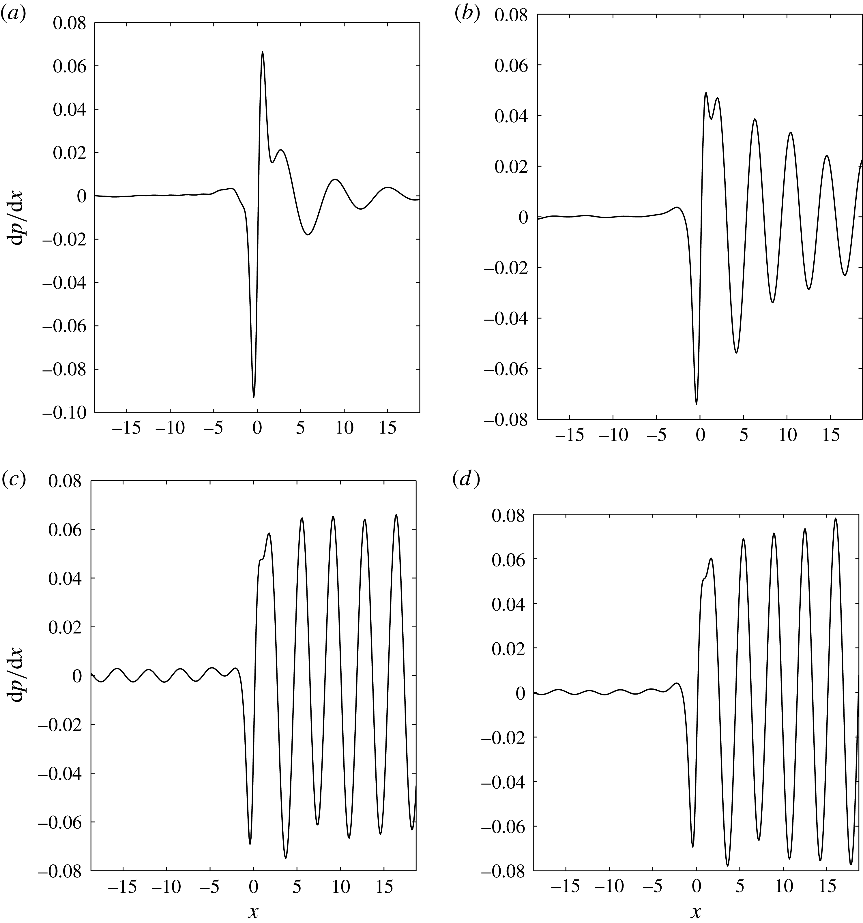
Figure 10. Pressure gradient distribution for
![]() $h=0.2$
and
$h=0.2$
and
![]() $K_{\infty }=-1$
: (
$K_{\infty }=-1$
: (
![]() $a$
)
$a$
)
![]() ${\it\omega}=1.7$
; (
${\it\omega}=1.7$
; (
![]() $b$
)
$b$
)
![]() ${\it\omega}=2.8$
; (
${\it\omega}=2.8$
; (
![]() $c$
)
$c$
)
![]() ${\it\omega}=3.35$
; (
${\it\omega}=3.35$
; (
![]() $d$
)
$d$
)
![]() ${\it\omega}=3.45$
.
${\it\omega}=3.45$
.

Figure 11. The receptivity coefficients
![]() $\mathscr{K}$
for negative values of the Kármán–Guderley parameter
$\mathscr{K}$
for negative values of the Kármán–Guderley parameter
![]() $K_{\infty }$
.
$K_{\infty }$
.
6.4. Transonic interaction law for
 $K_{\infty }>0$
For positive values of the Kármán–Guderley parameter, we treat the upper-deck equation (6.14a
) in a slightly different way. We start as before by representing the solution in the time-periodic form (6.18) and use the transformation (6.21), this time without scaling of the independent variable
![]() $Y$
. This results in the ‘telegraph equation’:
$Y$
. This results in the ‘telegraph equation’:
This has to be solved with the boundary condition
where
A fundamental solution of (6.41) may be sought in the form
Substitution of (6.44) into (6.41) leads to the Bessel equation
This means that the solution of (6.41) may be written as
where
![]() $\text{J}_{0}$
is the Bessel function. To find the function
$\text{J}_{0}$
is the Bessel function. To find the function
![]() ${\it\varphi}({\it\xi})$
, one has to use the boundary condition (6.42). Differentiation of (6.46) with respect to
${\it\varphi}({\it\xi})$
, one has to use the boundary condition (6.42). Differentiation of (6.46) with respect to
![]() $Y$
yields
$Y$
yields
Setting
![]() $Y=0$
in (6.47) and using (6.42) and (6.43) it is easily found that
$Y=0$
in (6.47) and using (6.42) and (6.43) it is easily found that
It remains to substitute (6.48) into (6.46), and we can see that the pressure in the viscous sublayer is given by
 $$\begin{eqnarray}\displaystyle \widetilde{P}(x) & = & \displaystyle \text{e}^{-\text{i}({\it\omega}/K_{\infty })x}p_{v}|_{Y=0}\nonumber\\ \displaystyle & = & \displaystyle -\frac{1}{\sqrt{K_{\infty }}}\int _{-\infty }^{x}\text{e}^{-\text{i}({\it\omega}/K_{\infty })(x-{\it\xi})}\widetilde{A}^{\prime \prime }({\it\xi})\text{J}_{0}\left(\frac{{\it\omega}}{K_{\infty }}(x-{\it\xi})\right)\text{d}{\it\xi}.\end{eqnarray}$$
Equation (6.49) was used, together with (6.16) and (6.17), to analyse the receptivity process for
![]() $K_{\infty }>0$
.
$K_{\infty }>0$
.
Similar to the subsonic flow regime, the calculations were performed for the roughness shape
![]() $g(x)=hF(x)$
with
$g(x)=hF(x)$
with
![]() $F(x)=\text{e}^{-2x^{2}}$
. The results of the calculations are shown in figure 12 in the form of the distribution of the pressure gradient along the body surface. We see that the Tollmien–Schlichting wave decays downstream if the acoustic wave interacting with the roughness has a subcritical frequency (
$F(x)=\text{e}^{-2x^{2}}$
. The results of the calculations are shown in figure 12 in the form of the distribution of the pressure gradient along the body surface. We see that the Tollmien–Schlichting wave decays downstream if the acoustic wave interacting with the roughness has a subcritical frequency (
![]() ${\it\omega}=2.6$
) and grows for a supercritical frequency (
${\it\omega}=2.6$
) and grows for a supercritical frequency (
![]() ${\it\omega}=3.25$
). The results in figure 12(a) correspond to unit value of Kármán–Guderley parameter
${\it\omega}=3.25$
). The results in figure 12(a) correspond to unit value of Kármán–Guderley parameter
![]() $K_{\infty }$
. Figure 12(b) shows that for
$K_{\infty }$
. Figure 12(b) shows that for
![]() $K_{\infty }=1$
the neutral frequency is
$K_{\infty }=1$
the neutral frequency is
![]() ${\it\omega}=3.025$
.
${\it\omega}=3.025$
.
The calculations were repeated for a number of values of the Kármán–Guderley parameter in the range
![]() $K_{\infty }\in (0,5)$
, and for various values of the roughness height
$K_{\infty }\in (0,5)$
, and for various values of the roughness height
![]() $h$
. The results of these calculations are summarised in figure 13, where the receptivity coefficient
$h$
. The results of these calculations are summarised in figure 13, where the receptivity coefficient
![]() $\mathscr{K}$
for neutral Tollmien–Schlichting waves is displayed. Interestingly, the receptivity coefficient does not show the same growth with
$\mathscr{K}$
for neutral Tollmien–Schlichting waves is displayed. Interestingly, the receptivity coefficient does not show the same growth with
![]() $h$
as for the subsonic flow regime (see figure 11).
$h$
as for the subsonic flow regime (see figure 11).
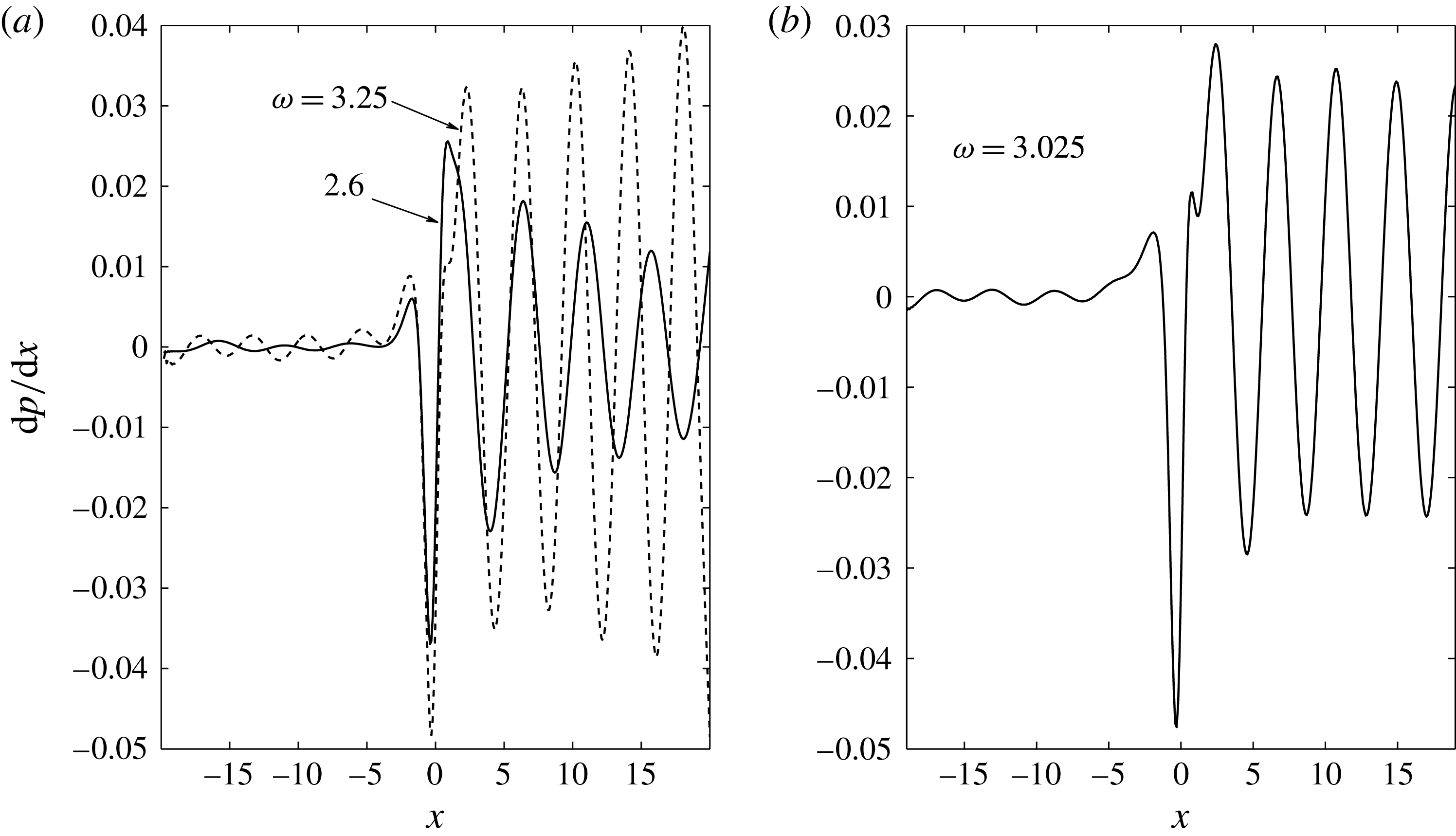
Figure 12. Pressure gradient distribution for three different acoustic wave frequencies
![]() ${\it\omega}$
, roughness hump height
${\it\omega}$
, roughness hump height
![]() $h=0.1$
and Kármán–Guderley parameter
$h=0.1$
and Kármán–Guderley parameter
![]() $K_{\infty }=1$
: (a) subcritical and supercritical frequencies; (b) neutral perturbations.
$K_{\infty }=1$
: (a) subcritical and supercritical frequencies; (b) neutral perturbations.

Figure 13. The receptivity coefficient
![]() $\mathscr{K}$
for
$\mathscr{K}$
for
![]() $K_{\infty }>0$
.
$K_{\infty }>0$
.
7. Discussion of the results
This work is concerned with the generation of the Tollmien–Schlichting waves in the boundary layer on a wing surface in the transonic flow regime. Assuming that the Reynolds number is large, we use the transonic version of the viscous–inviscid interaction theory, which is known to describe the stability of the boundary layer on the lower branch of the neutral curve. It is assumed that the Tollmien–Schlichting wave is generated through interaction of the acoustic wave impinging upon the boundary layer with steady flow perturbations produced in the flow by a small wall roughness. The results of the analysis confirm, once again, that effective generation of the Tollmien–Schlichting waves takes place when the so-called double-resonance condition is observed. This condition requires that (i) the frequency of the acoustic wave is tuned to the frequency of the Tollmien–Schlichting wave, and (ii) in the Fourier spectrum of the steady perturbations produced by the wall roughness there is a harmonic with wavenumber that coincides with the wavenumber of the Tollmien–Schlichting wave. The transonic version of the triple-deck theory is applicable when the free-stream Mach number
![]() $M_{\infty }$
is such that
$M_{\infty }$
is such that
![]() $M_{\infty }-1=O(\mathit{Re}^{-1/9})$
. In this flow regime, the dimensionless frequency of the Tollmien–Schlichting wave is an
$M_{\infty }-1=O(\mathit{Re}^{-1/9})$
. In this flow regime, the dimensionless frequency of the Tollmien–Schlichting wave is an
![]() $O(\mathit{Re}^{2/9})$
quantity and wavelength is estimated as
$O(\mathit{Re}^{2/9})$
quantity and wavelength is estimated as
![]() $O(\mathit{Re}^{-1/3})$
.
$O(\mathit{Re}^{-1/3})$
.
We first develop the linear receptivity theory. It is applicable when the amplitude of the pressure perturbation in the acoustic wave is small compared to
![]() ${\it\rho}_{\infty }U_{\infty }^{2}\mathit{Re}^{-1/9}$
, and the roughness height is small compared to
${\it\rho}_{\infty }U_{\infty }^{2}\mathit{Re}^{-1/9}$
, and the roughness height is small compared to
![]() $L\mathit{Re}^{-11/18}$
. Under these conditions, the governing equations my be solved in an analytic form. As a result, an explicit formula for the amplitude of the generated Tollmien–Schlichting wave is deduced. It can be expressed as the product of the so-called receptivity coefficient and the Fourier transform of the roughness shape calculated for wavenumber of the Tollmien–Schlichting wave. The former does not depend on the roughness shape, and reaches a maximum when the Kármán–Guderley parameter
$L\mathit{Re}^{-11/18}$
. Under these conditions, the governing equations my be solved in an analytic form. As a result, an explicit formula for the amplitude of the generated Tollmien–Schlichting wave is deduced. It can be expressed as the product of the so-called receptivity coefficient and the Fourier transform of the roughness shape calculated for wavenumber of the Tollmien–Schlichting wave. The former does not depend on the roughness shape, and reaches a maximum when the Kármán–Guderley parameter
![]() $K_{\infty }$
becomes zero or, equivalently, the free-stream Mach number
$K_{\infty }$
becomes zero or, equivalently, the free-stream Mach number
![]() $M_{\infty }=1$
.
$M_{\infty }=1$
.
In the second part of the paper, we lift the restriction on the roughness height, allowing the basic flow to develop a local separation region near the roughness. For this case the analysis of the generation of the Tollmien–Schlichting waves is conducted through numerical solution of the viscous–inviscid interaction problem. First, the basic steady flow is calculated for various values of the Kármán–Guderley parameter
![]() $K_{\infty }$
, progressively increasing the roughness height. Then the flow response to the impinging acoustic wave is determined through numerical solution of the unsteady viscous–inviscid interaction problem. The numerical method used in this study is based on Newtonian iterations where the solutions in the viscous and inviscid parts of the flow are calculated assuming that the displacement function is known. The iterations are conducted to adjust the displacement function such that it would make the pressure distributions in the viscous and inviscid flow coincide with one another. The results of the calculations show that for negative
$K_{\infty }$
, progressively increasing the roughness height. Then the flow response to the impinging acoustic wave is determined through numerical solution of the unsteady viscous–inviscid interaction problem. The numerical method used in this study is based on Newtonian iterations where the solutions in the viscous and inviscid parts of the flow are calculated assuming that the displacement function is known. The iterations are conducted to adjust the displacement function such that it would make the pressure distributions in the viscous and inviscid flow coincide with one another. The results of the calculations show that for negative
![]() $K_{\infty }$
, when the flow outside the boundary layer is subsonic, the receptivity is enhanced significantly by the formation of a separation region. Surprisingly, in the supersonic flow regime (
$K_{\infty }$
, when the flow outside the boundary layer is subsonic, the receptivity is enhanced significantly by the formation of a separation region. Surprisingly, in the supersonic flow regime (
![]() $K_{\infty }>0$
) the separation has only a moderate effect on the receptivity process.
$K_{\infty }>0$
) the separation has only a moderate effect on the receptivity process.
In conclusion, we shall make the following comment. The asymptotic approach used in this paper is primarily intended to uncover the fundamental physical processes involved in the receptivity process. At the same time, we know from a number of comparisons of the triple-deck theory with the Navier–Stokes simulations of the boundary-layer receptivity in subsonic flows that the triple-deck predictions are rather accurate (see e.g. Tumin Reference Tumin2006; Tullio & Ruban Reference Tullio and Ruban2015). Therefore, we expect the results presented in this paper to be sufficiently accurate for engineering applications.
Acknowledgements
This research was performed in the Laminar Flow Control Centre (LFC-UK) at Imperial College London. The centre is supported by EPSRC, Airbus UK and EADS Innovation Works.


