


1. Introduction
In plane Poiseuille flow, transition to turbulence often arises for Reynolds numbers not greater than the critical value for linear stability analysis,  $Re = 5772$. For Reynolds numbers consistently lower than this threshold value obtained by linear analysis, the flow may exhibit localised turbulence (Tsukahara et al. Reference Tsukahara, Seki, Kawamura and Tochio2005). Carlson, Widnall & Peeters (Reference Carlson, Widnall and Peeters1982) first observed laminar–turbulent patterns in channel flow, for
  $Re = 1000$. In very large domains, localised turbulent bands embedded in the laminar flow, tilted with respect to the streamwise direction, are observed (Tsukahara, Kawaguchi & Kawamura Reference Tsukahara, Kawaguchi and Kawamura2014; Xiong et al. Reference Xiong, Tao, Chen and Brandt2015; Tao, Eckhardt & Xiong Reference Tao, Eckhardt and Xiong2018; Shimizu & Manneville Reference Shimizu and Manneville2019; Kashyap, Duguet & Dauchot Reference Kashyap, Duguet and Dauchot2020b). In channel flow, Kashyap et al. (Reference Kashyap, Duguet and Dauchot2020b) have found that the mean angle of the bands remains approximately constant (
 $\theta \approx 25^\circ$) for a friction Reynolds number ranging from
  $60< Re_\tau < 90$, while increasing towards
  $\theta \approx 45^\circ$ for
  $Re_\tau <60$. This oblique laminar–turbulent pattern is also observed in other shear flows, although for a different range of Reynolds numbers and presenting different angles (Prigent et al. Reference Prigent, Grégoire, Chaté, Dauchot and van Saarloos2002; Barkley & Tuckerman Reference Barkley and Tuckerman2005; Duguet, Schlatter & Henningson Reference Duguet, Schlatter and Henningson2010; Tuckerman & Barkley Reference Tuckerman and Barkley2011; Duguet & Schlatter Reference Duguet and Schlatter2013; Chantry, Tuckerman & Barkley Reference Chantry, Tuckerman and Barkley2017; Tuckerman, Chantry & Barkley Reference Tuckerman, Chantry and Barkley2020). Using numerical simulations, Tao et al. (Reference Tao, Eckhardt and Xiong2018) have established that oblique turbulent bands may arise in channel flow at
  $Re \approx 660$. Recently, forcing the flow with an inflectional instability, Song & Xiao (Reference Song and Xiao2020) have been able to generate turbulent bands at
  $Re\approx 500$, although not self-sustained. Turbulent bands in large domains have been analysed by several authors with the aim of studying their characteristics, such as their angle and length (Tsukahara et al. Reference Tsukahara, Seki, Kawamura and Tochio2005; Tao et al. Reference Tao, Eckhardt and Xiong2018; Kashyap et al. Reference Kashyap, Duguet and Dauchot2020b), as well as their dynamics and interactions (Duguet et al. Reference Duguet, Schlatter and Henningson2010; Tao et al. Reference Tao, Eckhardt and Xiong2018; Shimizu & Manneville Reference Shimizu and Manneville2019; Gomé, Tuckerman & Barkley Reference Gomé, Tuckerman and Barkley2020). In order to reduce the computational cost and the flow complexity, Barkley & Tuckerman (Reference Barkley and Tuckerman2005, Reference Barkley and Tuckerman2007) studied the behaviour of the plane Couette flow in a small domain tilted perpendicularly to the turbulent band direction. Later, Tuckerman et al. (Reference Tuckerman, Kreilos, Schrobsdorff, Schneider and Gibson2014) extended this methodology to plane Poiseuille flow.
Recently, many works have focused on the origin and growth of turbulent bands. By means of direct numerical simulations (DNSs) in a large-sized channel flow, Shimizu & Manneville (Reference Shimizu and Manneville2019) observed that the turbulent bands are characterised by an active region at the head, where streaks are generated, whereas streak decay is found in the tail. Based on these observations, they suggest that streak generation could be the origin of the self-sustaining process of a single turbulent band. Inspired by this conjecture, Xiao & Song (Reference Xiao and Song2020) have performed a linear stability analysis of the flow averaged in three different regions at the head of the band. They found an inflectional spanwise instability, which generates streaky structures similar to those found at the head of a turbulent band. Thus, they conjectured that an inflectional instability at the head of the turbulent band can be at the origin of its growth and sustainment. Based on this hypothesis, Song & Xiao (Reference Song and Xiao2020) have applied to the flow a volume forcing inducing inflectional instability, which was capable of triggering turbulence in the form of turbulent bands at low values of the Reynolds number. They observed a rapid non-modal growth of perturbations of the velocity profiles deformed by this continuous forcing. Using a nonlinear approach, Paranjape, Duguet & Hof (Reference Paranjape, Duguet and Hof2020) have searched for an edge state (i.e. a relative attractor populating the laminar–turbulent separatrix; see Skufca, Yorke & Eckhardt Reference Skufca, Yorke and Eckhardt2006) in a tilted domain and they have found a localised nonlinear travelling wave solution that shows properties very similar to those of turbulent bands in a tilted domain. In particular, turbulent bands are characterised by a small-scale flow within the turbulent region, composed of streaks and vortices, which is surrounded by a large-scale flow constituted of vortices parallel to the turbulent bands and having opposite direction on their two sides. This large-scale flow appears fundamental for the development of the turbulent band, as argued by Duguet & Schlatter (Reference Duguet and Schlatter2013), who employed the conservation of mass to propose that this large-scale flow is responsible for the turbulent band oblique evolution (see also Kashyap, Duguet & Chantry Reference Kashyap, Duguet and Chantry2020a).
Based on these and others observations, Tao et al. (Reference Tao, Eckhardt and Xiong2018) suggested that, for triggering and sustaining a turbulent band, a large-scale flow is necessary. Moreover, they reported a strong increase of the total disturbance kinetic energy corresponding to the generation of turbulent bands. This energy increase follows a quasi-algebraic growth, instead of an exponential behaviour, as should be expected in the case of asymptotic instability as that reported by Xiao & Song (Reference Xiao and Song2020). It has been known since the pioneering work of Landahl (Reference Landahl1980) that algebraic kinetic energy growth of perturbations is induced when weak counter-rotating vortices generate high-amplitude streaky structures by means of the lift-up mechanism. These two flow structures, which are easily retrieved by optimal transient growth analysis (Luchini Reference Luchini2000), are two of the fundamental elements of the self-sustaining process which supports turbulence in shear flows (Hamilton, Kim & Waleffe Reference Hamilton, Kim and Waleffe1995; Waleffe Reference Waleffe1997), together with secondary instability of the streaks which is linked to the generation of inflectional points in the velocity profiles. Despite the observation of a consistent kinetic energy growth together with streaks generation at the head of a turbulent band, the possible relations between turbulent bands generation, the optimal energy growth of streaks and their inflectional instability, have still not been investigated in the literature.
The aim of this study is to elucidate the possible link between transient energy growth mechanisms and the generation and sustaining of turbulent bands in channel flow. For investigating the energy growth mechanism in detail, we focus our analysis on a tilted domain allowing the generation of a single localised turbulent band, as done previously in DNSs (Tuckerman et al. Reference Tuckerman, Kreilos, Schrobsdorff, Schneider and Gibson2014).
In this study, we search for linear (Luchini Reference Luchini2000; Cherubini et al. Reference Cherubini, De Tullio, De Palma and Pascazio2013) and nonlinear optimal perturbations (Pringle & Kerswell Reference Pringle and Kerswell2010; Cherubini et al. Reference Cherubini, De Palma, Robinet and Bottaro2010, Reference Cherubini, De Palma, Robinet and Bottaro2011; Monokrousos et al. Reference Monokrousos, Bottaro, Brandt, Di Vita and Henningson2011; Cherubini et al. Reference Cherubini, De Palma, Robinet and Bottaro2012; Pringle, Willis & Kerswell Reference Pringle, Willis and Kerswell2012; Rabin, Caulfield & Kerswell Reference Rabin, Caulfield and Kerswell2012; Cherubini & De Palma Reference Cherubini and De Palma2013; Duguet & Schlatter Reference Duguet and Schlatter2013) for the channel flow in a tilted domain at  $Re=1000$. We find that transient growth of streaks is able to generate turbulent bands, although only in the presence of a large-scale flow arising from spatial localisation.
The paper is organised in the following way. The problem formulation is presented in § 2. Then, in § 3 the linear and nonlinear optimal perturbations are shown and discussed. Finally, conclusions are drawn in § 4.
2. Problem formulation
For reducing the problem complexity and the computational cost, a tilted domain is considered for analysing oblique turbulent bands in plane Poiseuille flow, as done previously by Barkley & Tuckerman (Reference Barkley and Tuckerman2005, Reference Barkley and Tuckerman2007) for plane Couette flow and by Tuckerman et al. (Reference Tuckerman, Kreilos, Schrobsdorff, Schneider and Gibson2014) for plane Poiseuille flow. Starting from the classical plane Poiseuille flow,  $\boldsymbol {U}_P = [U_P(y), 0, 0]^{\rm T}$, with
  $U_P (y) = 1-y^2$, defined in the coordinate system
  $\boldsymbol {x}'=(x',y',z')^{\rm T}$, where
  $x'$ indicates the direction of the flow
  $U_P$, the tilted domain is obtained by applying the following change of reference:
 \begin{equation} \boldsymbol{\hat{e}}_{x} = \cos \theta \boldsymbol{\hat{e}}_{x'} - \sin \theta \boldsymbol{\hat{e}}_{z'}, \quad \boldsymbol{\hat{e}}_{y} = \boldsymbol{\hat{e}}_{y'}, \quad \boldsymbol{\hat{e}}_{z} = \sin \theta \boldsymbol{\hat{e}}_{x'} + \cos \theta \boldsymbol{\hat{e}}_{z'}, \end{equation}
 $\boldsymbol {x}=(x,y,z)^{\rm T}$ being the tilted domain coordinate system, and
  $\theta$ being the angle between the two coordinates systems, corresponding to the angle of a turbulent band with respect to the flow direction, and
  $y=y'$.
The dynamics of the turbulent bands in the tilted domain can be described by decomposing the instantaneous field into a perturbation  $\boldsymbol {u}' = [u',v',w']^{\rm T}$ and a laminar base flow
  $\boldsymbol {U} = [U(y), 0, W(y)]^{\rm T}$, with
  $U(y) = U_P(y) \cos \theta$ and
  $W(y) = U_P(y) \sin \theta$. The perturbation dynamics is governed by the non-dimensional Navier–Stokes equations for incompressible flows, written in a perturbative form with respect to the base flow:
 \begin{equation} \displaystyle \frac{\partial u_i'}{\partial x_i} = 0, \quad \displaystyle \frac{\partial u_i'}{\partial t} + u_j'\frac{\partial u_i'}{\partial x_j} + u_j' \frac{\partial U_i}{\partial x_j} + U_j \frac{\partial u_i'}{\partial x_j} ={-} \frac{\partial p'}{\partial x_i} + \frac{1}{Re} \frac{\partial^2 u_i'}{\partial x_j^2}, \end{equation}
where  $p'$ is the pressure perturbation and
  $Re = U_{c} h / \nu$ is the Reynolds number defined using the centreline velocity of the laminar Poiseuille flow,
  $U_c$, the half-width of the channel,
  $h$, and the kinematic viscosity
  $\nu$.
In order to find the optimal solution able to trigger turbulent bands in the tilted domain, we have computed linear and nonlinear optimal perturbations (Cherubini et al. Reference Cherubini, De Palma, Robinet and Bottaro2010; Pringle et al. Reference Pringle, Willis and Kerswell2012). In both cases, we choose as objective function the energy gain  $G(T) = E(T)/E(0)$, where
  $E(t)=1/(2V)\int \sum {u_i'}^2(t) \,{\rm d}V$,
  $E(T)$ and
  $E(0)$ being the kinetic energy at the chosen target time,
  $T$, and at the initial time, respectively. Thus, we search for the initial perturbation
  $\boldsymbol {u}'(0)$ providing the largest possible energy at target time
  $T$ with an optimisation loop based on the Lagrange multiplier technique (Cherubini et al. Reference Cherubini, De Palma, Robinet and Bottaro2011). Linear optimisation is carried out using an in-house Matlab code, whereas nonlinear optimisation is implemented within the open source code
  $Channelflow$ (channelflow.ch) (Gibson et al. Reference Gibson2021).
For all the simulations, the volume flow rate is kept constant imposing the bulk velocity equal to  $U_{bulk} = 2/3$. The same domain size and spatial discretisation used by Tuckerman et al. (Reference Tuckerman, Kreilos, Schrobsdorff, Schneider and Gibson2014) is adopted, namely
  $L_x \times L_y \times L_z = 10 \times 2 \times 40$ discretised using a
  $N_x \times N_y \times N_z = 128 \times 65 \times 512$ grid. All computations are performed at
  $Re = 1000$, for which Tuckerman et al. (Reference Tuckerman, Kreilos, Schrobsdorff, Schneider and Gibson2014) have reported a persisting turbulent-laminar pattern in the form of a single band. The angle of the tilted domain,
  $\theta$, is chosen to be equal to
  $35^{\circ }$ in accordance with that numerically observed at
  $Re = 1000$ by Kashyap et al. (Reference Kashyap, Duguet and Dauchot2020b) in large domains.
3. Results
First, a DNS is performed at  $Re = 1000$ in the tilted domain. In figure 1(a), a snapshot of the perturbation field is shown. As done previously by other authors, the flow with a higher Reynolds number, for which turbulence occupies the whole domain, is simulated. Then, the Reynolds number is reduced slowly until
  $Re = 1000$, reaching the laminar–turbulent pattern shown in figure 1(a). As already discussed by Tuckerman et al. (Reference Tuckerman, Kreilos, Schrobsdorff, Schneider and Gibson2014) for a tilted domain with the same size and Reynolds number, the turbulent state appears in the form of one turbulent band. In the instantaneous field, oblique wave-like structures such as alternating low- and high-speed streaks, are observed within the turbulent band and at its head. As expected, these structures present an angle with respect to the
  $x$ direction comparable to that of the base flow, and resemble the streaks observed at the head of a turbulent band in large (non-tilted) domains (Shimizu & Manneville Reference Shimizu and Manneville2019; Liu et al. Reference Liu, Xiao, Zhang, Li, Tao and Xu2020). Inspecting the premultiplied energy spectra of the streamwise instantaneous velocity provided in figures 1(b) and 1(c), we found an energy peak at
  $k_x \approx \pm 1.27$ and
  $k_z \approx \pm 1.6$. Thus, as discussed previously, the flow is dominated by oblique structures with angle of approximately
  $\arctan (k_x/k_z) \approx \pm 38^{\circ }$.

Figure 1. (a) Isosurface of negative streamwise velocity ( $u = -0.16$, yellow) and Q-criterion (
 $Q = 0.05$) coloured by the streamwise vorticity (positive red, negative blue) of a turbulent-laminar pattern at
  $Re=1000$ in a domain tilted with
  $\theta =35^{\circ }$. (b), (c) Logarithm of the premultiplied spectral energy versus the wall-normal distance
  $y$ for the instantaneous field in (a): (b)
  $k_x E_{uu}(k_x)$; (c)
  $k_z E_{uu}(k_z)$. The white ‘X’ symbols indicate the energy peaks.
In order to understand the origin of these oblique structures and the main mechanisms responsible for the generation of a turbulent band, a linear optimisation of perturbations in the tilted domain is first performed. As the base flow varies only in the wall-normal direction, we optimise the kinetic energy of sinusoidal perturbations, with given wavenumbers  $k_x$ and
  $k_z$ in the
  $x$ and
  $z$ direction, respectively, constrained by (2.2a,b) linearised with respect to the base flow.
3.1. Linear optimal perturbations
The linear optimisation problem was solved at  $Re = 1000$ for streamwise and spanwise wavenumbers in the range
  $0< k_x<2$,
  $-3< k_z<3$. Figure 2(a) provides the variation of the optimal gain with the spanwise and streamwise wavenumbers.

Figure 2. (a) Contours of the linear optimal gain  $G$ versus the streamwise (
 $k_x$) and spanwise (
 $k_z$) wavenumbers, for
  $Re=1000$ in the domain tilted with angle
  $\theta = 35^{\circ }$. The red cross indicates the optimal growth
  $G_{opt}$. (b) Streamwise velocity component of the initial linear optimal perturbation for
  $T= T_{opt} = 74.6$,
  $k_x = 1.19$ and
  $k_z = -1.71$.
The maximum growth is achieved at the optimal target time  $T_{opt} = 74.6$, for
  $k_x = 1.19$ and
  $k_z = -1.71$, leading to an optimal gain
  $G_{opt}=196.07$. As should be expected, the optimal gain, time and wavenumbers are very close to those found by Reddy & Henningson (Reference Reddy and Henningson1993) for the plane Poiseuille flow, once reported to a tilted domain. Note also that similar values of streamwise and spanwise wavenumbers have been found by Xiao & Song (Reference Xiao and Song2020) performing a linear stability analysis around the mean flow in a region at the head of the turbulent band. Moreover, the optimal streamwise and spanwise wavenumbers are very close to the ones for which the premultiplied energy spectra in figures 1(b) and 1(c) present a peak. Thus, these optimal perturbations can be linked to the oblique waves observed at the head of the turbulent band. As shown in figure 2(b), the linear optimal perturbation is oblique with angle equal to
  $\arctan (k_x/k_z) \approx -35^{\circ }$, in accordance to the classical plane Poiseuille flow (Reddy & Henningson Reference Reddy and Henningson1993), and modulated in both periodic directions. This had to be expected because the base flow presents a crossflow component, in analogy with the shear flow developing on a swept-wing, whose unstable modes and optimal perturbations are characterised by cross-flow vortices, namely three-dimensional oblique vortical perturbations with negative spanwise wavenumber. As shown in figure 3(a), at
  $t=0$ the linear optimal perturbation shows counter-rotating vortices with a large wall-normal component, which decreases in time towards the target time (see figure 3b), whereas the streamwise and spanwise components strongly increase creating oblique streaks. The mechanism creating these oblique energetic structures is based on the transport of the wall-normal shear of both streamwise and spanwise component of the base flow, which may be seen as a tilted counterpart of the lift-up effect.

Figure 3. Velocity profiles of different optimal disturbances at (a), (c), (e)  $t=0$ and at (b), (d), (f) target time: (a), (b) linear optimal computed for
  $k_x = 1.2$,
  $k_z = -1.75$ and
  $T_{opt} = 73.11$; (c), (d) nonlinear optimal at the lowest energy (among the considered ones) able to trigger turbulence, obtained for
  $E_0=2.1\times 10^{-5}$,
  $T=10$ and for (e), (f)
  $E_0=1.4 \times 10^{-6}$ and
  $T = 75$. (a) Linear,
  $t=0$,
  $T=73.11$. (b) Linear,
  $t=T_{opt}=73.11$. (c) Nonlinear,
  $t=0$,
  $T=10$. (d) Nonlinear,
  $t=T=10$. (e) Nonlinear,
  $t=0$,
  $T=75$. (f) Nonlinear,
  $t=T=75$.
The linear optimal perturbation computed for  $T_{opt}$ is then injected into the laminar flow in the tilted domain with different values of the initial energy
  $E(0)$, in order to verify whether such a linear transient-growth mechanism could induce transition in the form of turbulent bands. In figure 4, the energy evolution in time is reported for the linear optimal perturbations with different initial energies (black lines). The perturbation with unitary energy norm is the only one able to induce the formation of the turbulent band, whereas the others lead to relaminarisation. However, it is observed that turbulence is at first triggered in the whole domain and only at very long time (
 ${O}(100)$) it localises in a band.

Figure 4. Kinetic energy time evolution for the linear optimal perturbation with  $E_0 = 0.01,0.1$ and
  $1$ (black lines) and for the artificially localised perturbation (red line) for
  $\sigma =2.5$ and
  $A=0.05$.
In order to ascertain that this behaviour is not due to the alignment of the optimal perturbation with respect to the base flow, we have performed a set of DNSs by superposing a subharmonic perturbation to the linear optimal one (Pralits, Bottaro & Cherubini Reference Pralits, Bottaro and Cherubini2015), such that
 \begin{equation} \boldsymbol{u}' = A_0 \boldsymbol{u}_{opt}(k_z,k_x) + A_1 \boldsymbol{u}_{opt}(k_z/2,k_x/2),\end{equation}
where  $A_0$ and
  $A_1$ have been varied among the values
  $[0.1,0.5,1.0,2.0,5.0,10.0]$. Figure 5 provides the isocontours of the time evolution of the wall-normal perturbation obtained for the case with
  $A_0=0.5$ and
  $A_1=0.5$, together with the normalised
  $y$-integrated flow
  $\overline {u_i} = 1/2 \int _{-1}^1 u_i \,{{\rm d} y}$. The inclined streaks rapidly experience breakdown, inducing small-scale vorticity and fluctuations in the whole domain. One can also note that no large-scale vortices in the
  $y$-integrated flow are observed (see Duguet & Schlatter (Reference Duguet and Schlatter2013) for the importance of large-scale flow in the turbulent band generation). Thus, the linear optimal perturbation induces turbulence in the whole domain even when superposed to a perturbation able to break its spatial symmetry but not providing a large-scale flow. Most probably, this behaviour is linked to the fact that the linear optimal disturbance is not spatially localised but occupies the whole domain, which also explains the large amount of energy needed for triggering turbulence by means of this optimal mechanism. In fact, it has been established that spatially localised perturbations are able to self-induce large-scale flow, provided that spanwise homogeneity is broken and the streamwise velocity is sheared (Wang et al. Reference Wang, Guet, Monchaux, Duguet and Eckhardt2020). To provide spatial localisation of the optimal perturbation, aiming at triggering the turbulent band, we extended the optimisation to the fully nonlinear equations, which usually provide a consistent spatial localisation (Cherubini et al. Reference Cherubini, De Palma, Robinet and Bottaro2010; Farano et al. Reference Farano, Cherubini, Robinet and De Palma2015, Reference Farano, Cherubini, Robinet and De Palma2016; Kerswell Reference Kerswell2018). Note that the nonlinear optimisation is performed in a fully three-dimensional framework, without any hypothesis on the perturbation wavenumbers.

Figure 5. Time evolution of the linear optimal perturbation superposed to its subharmonic according to (3.1) with  $A_0 = 0.5$ and
  $A_1 = 0.5$; shaded isocontours of the wall-normal perturbation and vectors of the
  $y$-integrated flow in the
  $y=0.25$ plane: (a)
  $t=0$; (b)
  $t=10$; (c)
  $t=20$; (d)
  $t=50$.
3.2. Nonlinear optimal perturbations
Nonlinear optimisation has been performed in the tilted domain for several initial energies and target times, ranging from  $T=10$, which is close to the characteristic eddy turnover time of structures in the buffer layer (Butler & Farrell Reference Butler and Farrell1993), up to
  $T=75$, which is close to the optimal time recovered by the linear optimisation. For the lowest value of the target time, the nonlinear optimal perturbation triggers localised turbulence already for
  $E_0 \ge 2.1 \times 10^{-5}$. The nonlinear optimal perturbation computed for
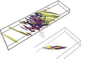
  $T=10$ and for the lowest (among those considered) input energy able to trigger turbulence is shown in figures 6(a) and 6(b) in a two- and three-dimensional view, respectively. As expected from previous works (Cherubini et al. Reference Cherubini, De Palma, Robinet and Bottaro2011; Monokrousos et al. Reference Monokrousos, Bottaro, Brandt, Di Vita and Henningson2011; Pringle et al. Reference Pringle, Willis and Kerswell2012), it is localised in one of the two periodic spatial directions. Furthermore, despite being an initial perturbation obtained optimising at a small (
 ${O}(10)$) target time with an energy which has not been bisected, it presents remarkable similarities with the edge state found by Paranjape et al. (Reference Paranjape, Duguet and Hof2020) in a tilted domain for
  $Re = 760$. Figure 6(a) shows the isocontours of the wall-normal perturbation, together with the normalised
  $y$-integrated large-scale flow
  $\overline {u_i} =1/2 \int _{-1}^1 u_i \,{{\rm d}y}$ for this optimal solution. One can observe a small-scale flow within a localised region, where the turbulent band will be generated, together with two larger-scale vortices surrounding this region, having opposite direction upstream and downstream of the localised perturbation. A large-scale vortical flow surrounding the region developing into a turbulent spot has been reported previously by several authors in both tilted and non-tilted domains (Kashyap et al. Reference Kashyap, Duguet and Chantry2020a). The three-dimensional visualisation in figure 6(b) shows that the small-scale flow consists of oblique streaks flanked by counter-rotating vortices. The streaks are aligned with the base flow, presenting an angle of approximately
  $35^{\circ }$ with respect to the streamwise direction, in accordance with the angle of the linear optimal perturbation.

Figure 6. Nonlinear optimal perturbations for  $Re = 1000$ and
  $t=0$ obtained for different initial energies and target times indicated in the subplots: (a), (c), (e), (g) shaded isocontours of the wall-normal perturbation and vectors of the
  $y$-integrated flow in the
  $y=0.25$ plane at
  $t=0$; (b), (d), (f), (h) isosurfaces of negative streamwise velocity (yellow) and
  $Q$-criterion coloured by the streamwise vorticity (positive red, negative blue) for
  $t=0$,
  $u = -0.01$,
  $Q = 0.02$. (a) 2D,
  $T=10$,
  $E_0 = 2.1\times 10^{-5}$. (b) 3D,
  $T=10$. (c) 2D,
  $T=25$,
  $E_0 = 4.6\times 10^{-6}$. (d) 3D,
  $T=25$. (e) 2D,
  $T=50$,
  $E_0 = 1.6\times 10^{-6}$. (f) 3D,
  $T=50$. (g) 2D,
  $T=75$,
  $E_0 = 1.4\times 10^{-6}$. (h) 3D,
  $T=75$.
As expected, this localised optimal perturbation evolves in time towards a turbulent band, as shown in figure 7(a). Note that this nonlinear optimal perturbation induces transition for an initial energy five orders of magnitude lower than that of the linear optimal one; this cannot be exclusively due to its spatial localisation. In fact, the wall-normal velocity profiles provided in figure 3(c) present strong differences with respect to their linear counterpart shown in figure 3(a). In particular, as typically observed in nonlinear optimal perturbations (Cherubini et al. Reference Cherubini, De Palma, Robinet and Bottaro2011), the streamwise velocity component is now of the same order of magnitude of the others, and the wall-normal component strongly changes. At target time (figure 3d), deformed streaks are obtained, presenting inflection points which might be linked to the inflectional instability discussed by Song & Xiao (Reference Song and Xiao2020).

Figure 7. Snapshots at  $t=600$ of the time evolution of the nonlinear optimal perturbations (NLOPs) obtained for
  $Re = 1000$, (a)
  $E_0 = 2.1 \times 10^{-5}$,
  $T = 10$ and (b)
  $E_0 = 1.5 \times 10^{-6}$,
  $T = 75$: isosurface of negative streamwise velocity (yellow) and
  $Q$-criterion coloured by the streamwise vorticity (positive red, negative blue) for
  $u = -0.15$,
  $Q = 0.5$.
Increasing the target time for the nonlinear optimisation, we found that the nonlinear optimal perturbation triggers localised turbulence for an even lower initial energy. In particular, for the largest target time, the nonlinear optimal perturbation is able to generate a turbulent band already at  $E_0 = 1.4 \times 10^{-6}$. Comparing figure 6(b,d,f,h), one can note that increasing the target time the nonlinear optimal perturbation further localises in all spatial directions (Cherubini et al. Reference Cherubini, De Palma, Robinet and Bottaro2011; Monokrousos et al. Reference Monokrousos, Bottaro, Brandt, Di Vita and Henningson2011; Pringle et al. Reference Pringle, Willis and Kerswell2012; Farano et al. Reference Farano, Cherubini, Robinet and De Palma2017). Note that the nonlinear optimal perturbations computed for
  $T=50$ and
  $T=75$ have a very similar shape and structure, and are able to induce localised turbulence for a very close value of the initial energy. The nonlinear optimal perturbation for
  $T=75$ and
  $E_0 = 1.4 \times 10^{-6}$, shown in a close-up in figure 6(h), consists of quasi-streamwise vortices alternated in the
  $x$–
$x$– $z$ directions, flanking patches of large streamwise perturbation. One can observe that this basic structure, which recalls that of the minimal seed for other shear flows (Rabin et al. Reference Rabin, Caulfield and Kerswell2012; Duguet et al. Reference Duguet, Monokrousos, Brandt and Henningson2013; Cherubini, De Palma & Robinet Reference Cherubini, De Palma and Robinet2015) appears to be spatially repeated within the optimal perturbations computed for lower target times and larger initial energies (see figures 6b and 6d). Moreover, comparing figures 6(a), 6(c), 6(e) and 6(g), one can observe that the large-scale structures characterising the
  $y$-integrated flow field become more spatially extended when
  $T$ is increased, filling almost the whole domain for the largest considered
  $T$ (smallest
  $E_0$). Also for this nonlinear perturbation, the wall-normal velocity profiles provided in figures 3(e) and 3(f) present strong differences with respect to their linear counterpart shown in figures 3(a) and 3(b) both at initial and at target times.
As expected, this localised optimal perturbation evolves in time towards a turbulent band, as shown by the three-dimensional view in figure 7(b). Figure 8 shows that the large-scale vortices present at initial time persist within the flow up to the creation of the turbulent band. Moreover, the localised wave packet evolving from the nonlinear optimal perturbation appears to be placed in the shear region between two counter-rotating large-scale vortices. Note that, as shown in figure 9, the kinetic energy rapidly increases up to  $t\approx 200$ (although a clear turbulent band can be observed already at
  $t\approx 100$) and then appears to reach a statistically steady value. Unlike linear ones, nonlinear optimal perturbations appear thus very efficient in inducing turbulent bands. However, it is still unclear whether it is the spatial localisation or rather the shape of the velocity profiles the key feature for the rapid generation of a turbulent band.

Figure 8. Time evolution of the nonlinear optimal perturbation for  $T = 75$ at different times; shaded contours of the wall-normal velocity and vectors of the
  $y$-integrated flow field at
  $y=0.25$: (a)
  $t=20$; (b)
  $t=50$; (c)
  $t=75$; (d)
  $t=100$; (e)
  $t=200$; (f)
  $t=300$.

Figure 9. Kinetic energy time-evolution of the nonlinear optimal perturbations obtained for different target times and initial energies.
3.3. Artificially localised perturbations
To isolate the effect of spatial localisation from the strong changes in the velocity profiles induced by the nonlinear effects, we enforced localisation in the  $z$ direction on the three-dimensional linear optimal solution shown in figure 2(b). This is achieved by multiplying the velocity components by a normal distribution having the form
 \begin{equation} f(z) = \exp\left({-\frac{1}{2}\frac{(z-z_0)^2}{\sigma^2}}\right), \end{equation}
where  $z_0 = 20$ represents the value at which the perturbation is centred, and different values of the standard deviation
  $\sigma$, ranging from
  $0.5$ to
  $5$, are considered. The resulting shapes of the normal distributions ensuring localisation in the
  $z$ direction, are shown in figure 10(a). After multiplying the velocity components of the (unit norm) linear optimal perturbation by
  $f(z)$ and by a given amplitude
  $A$, the incompressibility constraint is imposed by adjusting the spanwise perturbation in order to compensate for the non-solenoidal part of the artificially constructed perturbation. The resulting perturbation is then injected in the flow. Among the considered values of
  $A$, the lowest ones allowing transition to turbulence are provided in figure 10(b) for the different artificially localised perturbations, along with the corresponding initial energy for transition. One can observe that the amplitude needed for inducing transition decreases with increasing
  $\sigma$, indicating that less-localised perturbations need, in fact, a lower amplitude to trigger turbulence. However,
  $E_0$ is found to reach its minimum value for
  $\sigma =2.5$, for which the size of the initial perturbation roughly corresponds to that of the nonlinear optimal perturbation for
  $T=10$ (see figure 6a). This localised perturbation is injected in the DNS with the initial energy reported in figure 10(b), namely
  $E_0=1.39 \times 10^{-4}$. Its time evolution is reported in figure 11. First, the oblique streaks increase their amplitude (
 $t=20$) and start to saturate nonlinearly, until secondary instability arises (
 $t=50$) and triggers turbulence in a localised zone within the laminar flow (
 $t=80-100$). Although not very evident at
  $t=0$, two large-scale vortices can be clearly seen at
  $t=20$, and persist up to the creation of the localised band, the oblique streaks being placed in their shear region. At
  $t = 150$, the flow presents the same configuration shown in figure 1 for a turbulent band generated by decreasing the Reynolds number starting from a fully turbulent velocity field. Notably, inflection points similar to those observed in figure 3(d), are observed at small time in the velocity profiles. The corresponding time evolution of the kinetic energy, shown by the red line in figure 4, is rather similar to that of the nonlinear optimals provided in figure 9, showing a rapid increase of the energy followed by a slow saturation.

Figure 10. (a) Normal function  $f(z)$ for different values of the standard deviation. (b) Lowest amplitude (among the considered ones) for transition corresponding to different standard deviations with the corresponding initial energy.

Figure 11. Time evolution of the artificially localised linear optimal perturbation for  $\sigma =2.5$ and
  $A=0.05$ at different times; shaded contours of the wall-normal velocity at
  $y=0.25$: (a)
  $t=0$; (b)
  $t=20$; (c)
  $t=50$; (d)
  $t=80$; (e)
  $t=100$; (f)
  $t=150$. For visualisation purposes the initial perturbation has been shifted towards
  $z=0$.
Thus, we can infer that the differences in shape of the velocity profiles of the linear and nonlinear optimal perturbations are not crucial for the generation of the turbulence band, for which two main elements appear to be needed: (i) small-scale oblique streaks aligned with the baseflow, that saturate creating inflection points; (ii) spatial localisation in the  $z$ direction, which induces a large-scale vortical flow, as discussed by Wang et al. (Reference Wang, Guet, Monchaux, Duguet and Eckhardt2020). The transition at the small scale is due to the classical lift-up mechanism, followed by secondary instability of the saturated streaks, which triggers the self-sustained cycle supporting turbulence (Hamilton et al. Reference Hamilton, Kim and Waleffe1995; Waleffe Reference Waleffe1997). However, in the absence of a large-scale flow arising from spatial localisation and allowing to maintain the band, these mechanisms are not sufficient to generate localised turbulence. Of course, the initial phase of growth due to the lift-up mechanism can be skipped by directly feeding the flow with inflection points, as done by Song & Xiao (Reference Song and Xiao2020), but at the cost of a larger-amplitude disturbance.
In order to roughly evaluate the amplitude and spatial length of the large-scale flow needed to create the turbulent band, and to ascertain whether initial oblique vortices able to induce streaks are a key ingredient for this mechanism, we have initialised some computations using two large-scale vortices centred at  $(x_1, z_1) = (5,10)$,
  $(x_2, z_2) = (5,30)$, having the following analytical form:
 \begin{equation} u' ={-}\frac{A}{R} (z - z_0) {\rm e}^{-({r}/{2})},\quad w' ={-}\frac{A}{R} (x - x_0) {\rm e}^{-({r}/{2})}, \end{equation}
where  $r = ({(x-x_0)^2 + (z-z_0)^2})/{R^2}$,
  $A$ is the vortex amplitude and
  $R$ is the vortex radius. Note that these perturbations are not built to trigger the lift-up mechanism. The time evolution of the perturbations obtained for (i)
  $R=1$ and
  $A=2$, with
  $E_0 = 0.03127$, (ii)
  $R=5$ and
  $A=1$, with
  $E_0 = 0.0441$, and (iii)
  $R=10$ and
  $A=0.5$, with
  $E_0 = 0.0103$, are provided in figures 12, 13 and 14, respectively. We can observe that only the largest-radius perturbation directly leads to the formation of one localised band, whereas the other two perturbations generate two regions of localised turbulence, which either coalesce (see figure 12) or remain spatially separated until one of them decays (see figure 13). The time evolution of the kinetic energy, provided in figure 15, shows a steep decrease of the energy before saturation occurs, which is clearly due to the fact that the initial perturbation is not able to directly trigger a transient energy growth by means of the lift-up mechanism. It thus appears that large-scale vortices of radius comparable with the domain size might be sufficient for generating a turbulent band, but at the cost of a very large initial amplitude. The nonlinear optimisation procedure shows that a localised path of small-scale vortices able to trigger inclined streaks by means of the lift-up mechanism can generate turbulent bands for a much smaller amplitude. Thus, in the next section we focus on the artificially localised (linear optimal) perturbations, with the aim of verifying its capability of generating bands also in large, non-tilted domains, where no angle is imposed a priori.

Figure 12. Time evolution of two large-scale vortices with radius  $R = 1$ and amplitude
  $A = 2$: (a)
  $t=0$; (b)
  $t=10$; (c)
  $t=20$; (d)
  $t=50$; (e)
  $t=100$; (f)
  $t=500$. Contours and vectors as in figure 11.

Figure 13. Time evolution of two large-scale vortices with radius  $R = 5$ and amplitude
  $A = 1$: (a)
  $t=0$; (b)
  $t=10$; (c)
  $t=20$; (d)
  $t=50$; (e)
  $t=100$; (f)
  $t=500$. Contours and vectors as in figure 11.

Figure 14. Time evolution of two large-scale vortices with radius  $R = 10$ and amplitude
  $A = 0.5$: (a)
  $t=0$; (b)
  $t=10$; (c)
  $t=20$; (d)
  $t=50$; (e)
  $t=100$; (f)
  $t=500$. Contours and vectors as in figure 11.

Figure 15. Kinetic energy time evolution for the analytical large-scale perturbations.
3.4. Band generation in non-tilted domains
The artificially localised linear optimal perturbation computed in the tilted domain for  $\sigma =2.5$, has been injected in a very large (non-tilted) domain of size
  $L_{x'}\times L_{y'}\times L_{z'}=250\times 2\times 125$, and let it evolve freely by a DNS. As shown in figure 16, despite at
  $t=0$ a large-scale flow is present only in the vicinity of the perturbation, at
  $t=100$ a clear quadrupolar large-scale vortical structure, filling the whole domain, is observed. Note that, as discussed in Wang et al. (Reference Wang, Guet, Monchaux, Duguet and Eckhardt2020), a quadrupolar structure arises in the presence of a negative spanwise vorticity generated near the walls inside a spot, as a consequence of the shearing of the streamwise velocity and the breaking of the spanwise homogeneity. New streaky structures, generated by the self-sustained process triggered by the optimal counter-rotating vortices and streaks, are then created following the shear layer between two of the previously observed large-scale vortices (
 $t=300$), finally creating a clear turbulent band (
 $t=800$). Despite not being optimal for this large, non-tilted domain, this perturbation is able to generate a large-scale flow that promotes the formation of small-scale streaks in an oblique direction, consequently inducing the band formation. The optimisation of perturbations in this large non-tilted domain is beyond the scope of the present work, and is treated in detail in Parente et al. (Reference Parente, Robinet, De Palma and Cherubini2021), where the minimal-energy optimal perturbations able to generate turbulent bands are computed and discussed for different values of
  $Re$.
$Re$.

Figure 16. Time evolution of the artificially localised linear optimal perturbation reported in a large domain; contours of the wall-normal velocity and vectors of the  $y$-integrated large-scale flow (
 $\bar {u},\bar {w})$: (a)
  $t=0$; (b)
  $t=100$; (c)
  $t=300$; (d)
  $t=800$.
4. Conclusion
In this work we have investigated the energy growth mechanisms involved in the laminar–turbulent transition in the form of turbulent bands using linear and nonlinear optimisation. We have considered a plane Poiseuille flow at  $Re = 1000$ in a tilted domain with angle
  $\theta = 35^{\circ }$ that exhibits a single turbulent band. Linear optimisation in the tilted domain has shown that the optimal perturbation is three-dimensional and aligned with the oblique baseflow, in the form of low- and high-speed streaks modulated in the streamwise and spanwise directions with
  $k_x = 1.2$ and
  $k_z=- 1.75$, respectively. Similar wavenumbers are found at the same Reynolds number by DNS and by linear stability analysis at the head of the turbulent band, where an angle comparable to that of the optimal streaks is observed. However, the linear optimal perturbation needs a very large (
 ${O}(1)$) initial energy to trigger turbulence, which spreads in the whole domain.
Using nonlinear optimisation, even for a short target time, a localised turbulent band is triggered for an initial energy five orders of magnitude smaller. The nonlinear optimal perturbation, computed for several target times, is characterised by a localised small-scale flow and a large-scale flow surrounding it. The small-scale flow is composed by oblique counter-rotating vortices and streaks with an angle comparable to that found via linear optimisation, which develop inflection points at target time. For a sufficiently high target time, the nonlinear optimal perturbation is able to trigger a localised band for an initial energy as low as  ${O}(10^{-6})$. In order to separate the effect of the large-scale flow and localisation from that of the small-scale structures, which are responsible for the very low value of the initial energy able to induce the band, we have built a localised perturbation by artificially confining the linear optimal to a localised region in the
  $z$ direction and injected it into the laminar flow both in the tilted and in a non-tilted, very large domain. In both domains, a turbulent band is created. Turbulent bands are generated also when initialising the flow in the tilted domain by large-scale vortices alone, although for a very large initial energy, because in this last case the initial perturbation is not designed for triggering the lift-up effect.
These results suggest that transition to a turbulent band might arise due to the optimal lift-up mechanism when coupled with a large-scale vortical flow intimately linked to the spatial localisation of the disturbance. This energy growth mechanism provides high-amplitude streaks developing inflection points when saturating nonlinearly, but because the optimal streaks are aligned with the base flow, they cannot generate a turbulent band by themselves. Indeed, the large-scale flow induced by the spatial localisation of the perturbation provides the preferential direction of spreading of the streaks, and is thus necessary to trigger turbulence in the form of turbulent bands.
Funding
This work was granted access to the HPC resources of IDRIS under the allocation 2020- A0072A06362 and A0092A06362 made by GENCI. This work was partially funded by the grant PRIN2017-X7Z8S3 LUBRI-SMOOTH of the Italian Ministry of University and Research (MUR).
Declaration of interests
The authors report no conflict of interest.


