


1. Introduction
From the collection of coherent structures inhabiting turbulent flows the structures commonly called ‘vortices’ stand out because of their large coherence and relatively simple dynamics, when compared to other structures (Green Reference Green1995). Their importance is explained by their role in the transfers of mass, momentum and energy that take place in turbulent flows. These structures are often loosely defined as regions of concentrated vorticity and low pressure, with a lifetime that is usually considered to be large compared with the average characteristic time scale of the flow (Davidson Reference Davidson2015).
A subclass of these structures consists of the so-called intense vorticity structures (IVS) or ‘worms’ that constitute the smallest-scale eddies that can be found in a turbulent flow. They have often been defined as the structures having a vorticity magnitude that is above a certain threshold. Here, the threshold is set by the flow points with the highest vorticity magnitude that occupy
 $1\, \%$
of the total flow volume (following Jiménez et al. (Reference Jiménez, Wray, Saffman and Rogallo1993) and Jiménez & Wray (Reference Jiménez and Wray1998)). The worms are tubular structures with diameter
$1\, \%$
of the total flow volume (following Jiménez et al. (Reference Jiménez, Wray, Saffman and Rogallo1993) and Jiménez & Wray (Reference Jiménez and Wray1998)). The worms are tubular structures with diameter
 $D_{ivs } \approx 10\, \eta$
, where
$D_{ivs } \approx 10\, \eta$
, where
 $\eta$
is the Kolmogorov microscale. Their characteristic tangential velocity is
$\eta$
is the Kolmogorov microscale. Their characteristic tangential velocity is
 $U_{ivs} \approx u'$
, and their maximum vorticity magnitude is of the order of
$U_{ivs} \approx u'$
, and their maximum vorticity magnitude is of the order of
 $\omega _{ivs} \sim \omega '\, Re_{\lambda }^{1/2}$
, where
$\omega _{ivs} \sim \omega '\, Re_{\lambda }^{1/2}$
, where
 $\omega '$
and
$\omega '$
and
 $u'$
are the root-mean-square vorticity and velocity, respectively (Jiménez et al. Reference Jiménez, Wray, Saffman and Rogallo1993; Jiménez & Wray Reference Jiménez and Wray1998), while their length scales with the Kolmogorov microscale (
$u'$
are the root-mean-square vorticity and velocity, respectively (Jiménez et al. Reference Jiménez, Wray, Saffman and Rogallo1993; Jiménez & Wray Reference Jiménez and Wray1998), while their length scales with the Kolmogorov microscale (
 $L_{ivs} \sim \eta$
) as
$L_{ivs} \sim \eta$
) as
 $L_{ivs} \approx 60\, \eta$
(Ghira, Elsinga & da Silva Reference Ghira, Elsinga and da Silva2022). (Throughout this paper, we use the symbol ‘
$L_{ivs} \approx 60\, \eta$
(Ghira, Elsinga & da Silva Reference Ghira, Elsinga and da Silva2022). (Throughout this paper, we use the symbol ‘
 ${\sim}$
’ to imply scaling between two quantities even if this does not necessarily imply that they are of the same order.) It is noteworthy that direct numerical simulations (DNS) carried out at higher Reynolds numbers than previously available, with Taylor-based Reynolds numbers
${\sim}$
’ to imply scaling between two quantities even if this does not necessarily imply that they are of the same order.) It is noteworthy that direct numerical simulations (DNS) carried out at higher Reynolds numbers than previously available, with Taylor-based Reynolds numbers
 $Re_{\lambda } = 1100$
, have again confirmed visually that intense vorticity is organised into vortex tubes (Ishihara et al. Reference Ishihara, Kaneda, Yokokawa, Itakura and Uno2007; Buaria et al. Reference Buaria, Pumir, Bodenschatz and Yeung2019, Reference Buaria, Pumir and Bodenschatz2020).
$Re_{\lambda } = 1100$
, have again confirmed visually that intense vorticity is organised into vortex tubes (Ishihara et al. Reference Ishihara, Kaneda, Yokokawa, Itakura and Uno2007; Buaria et al. Reference Buaria, Pumir, Bodenschatz and Yeung2019, Reference Buaria, Pumir and Bodenschatz2020).
It has been reported that the kinetic energy content and the total viscous dissipation included in the core of these structures are both negligible (Jiménez et al. Reference Jiménez, Wray, Saffman and Rogallo1993; Jiménez & Wray Reference Jiménez and Wray1998); however, the most intense dissipation events within the flow field happen when two (or more) of these structures come close (Ganapathisubramani, Lakshminarasimhan & Clemens Reference Ganapathisubramani, Lakshminarasimhan and Clemens2008), and their study is motivated by flow problems as diverse as turbulent entrainment (da Silva, dos Reis & Pereira Reference da Silva, dos Reis and Pereira2011), internal intermittency (Ishihara et al. Reference Ishihara, Kaneda, Yokokawa, Itakura and Uno2007), mixing (Kida & Miura Reference Kida and Miura1998) and cloud physics (Shaw Reference Shaw2003).
The IVS have been investigated mainly in homogeneous isotropic turbulence (HIT) through the use of DNS (e.g. Siggia Reference Siggia1981; Kerr Reference Kerr1985; She, Jackson & Orszag Reference She, Jackson and Orszag1991; Vincent & Meneguzzi Reference Vincent and Meneguzzi1991, Reference Vincent and Meneguzzi1994; Ruetsch & Maxey Reference Ruetsch and Maxey1991; Jiménez et al. Reference Jiménez, Wray, Saffman and Rogallo1993; Jiménez & Wray Reference Jiménez and Wray1998; Ghira et al. Reference Ghira, Elsinga and da Silva2022), and also in experimental studies (e.g. Villermaux, Sixou & Gagne Reference Villermaux, Sixou and Gagne1995; Cadot, Douady & Couder Reference Cadot, Douady and Couder1995; Ganapathisubramani et al. Reference Ganapathisubramani, Lakshminarasimhan and Clemens2008; Aligolzadeh, Holzner & Dawson Reference Aligolzadeh, Holzner and Dawson2023). Other flow cases include also mixing layers (Tanahashi, Iwase & Miyauchi Reference Tanahashi, Iwase and Miyauchi2001), channel flows (Kang, Tanahashi & Miyauchi Reference Kang, Tanahashi and Miyauchi2008) and jets (Ganapathisubramani et al. Reference Ganapathisubramani, Lakshminarasimhan and Clemens2008; da Silva et al. Reference da Silva, dos Reis and Pereira2011), where the IVS have been shown to display similar characteristics, even when analysed using slightly different methods (see Ghira et al. (Reference Ghira, Elsinga and da Silva2022) and references therein).
In spite of the large number of works devoted to the investigation of the geometrical and dynamical characteristics of IVS, surprisingly few studies addressed the lifetime of these structures. It has been assumed for many years that the lifetime of the ‘worms’ is ‘long’, and it has often been implied that their lifetime is of the order of the integral time scale of the flow (Jiménez et al. Reference Jiménez, Wray, Saffman and Rogallo1993). The long lifetimes appear consistent with the fact that the cores of the IVS are well described by the steady Burgers vortex model. However, few, if any, reliable direct measurements of this lifetime have been made up to now. The difficulty is linked to the need to save for subsequent analysis many massive instantaneous velocity fields from DNS, and because of other technical difficulties in experimental studies.
Douady, Couder & Brachet (Reference Douady, Couder and Brachet1991) used cavitation in a liquid seeded with bubbles to investigate the regions of low pressure in the turbulent flow generated between two rotating disks. By tracking the regions of low pressure, which are strongly correlated with regions of intense vorticity magnitude, they were able to follow some vorticity structures. They observed that these structures are for the large part short-lived and display a high degree of temporal and spatial intermittency, and that the observed filaments exist only during one large-scale turnover time.
Villermaux et al. (Reference Villermaux, Sixou and Gagne1995) measured the lifetime of vortices generated in a water tank by oscillating disks at Taylor-based Reynolds numbers in the range
 $170 \lesssim Re_{\lambda } \lesssim 300$
. They report the lifetime to be about one-quarter of the integral time scale. However, they mention that their structures are very long filaments, with the size of the integral scale of motion, and that they are relatively few, with approximately one single structure per integral-scale cube volume. This suggests that these structures are much longer than the typical ‘worms’ described in DNS of isotropic turbulence (Ghira et al. Reference Ghira, Elsinga and da Silva2022).
$170 \lesssim Re_{\lambda } \lesssim 300$
. They report the lifetime to be about one-quarter of the integral time scale. However, they mention that their structures are very long filaments, with the size of the integral scale of motion, and that they are relatively few, with approximately one single structure per integral-scale cube volume. This suggests that these structures are much longer than the typical ‘worms’ described in DNS of isotropic turbulence (Ghira et al. Reference Ghira, Elsinga and da Silva2022).
To the authors’ knowledge, the only systematic attempt at measuring the lifetime of the eddy structures in DNS was carried out by Biferale, Scagliarini & Toschi (Reference Biferale, Scagliarini and Toschi2010) using isotropic turbulence with Taylor-based Reynolds number in the range
 $65 \lesssim Re_{\lambda } \lesssim 185$
. They use an indirect procedure based on following light particles trapped inside vortex filaments, and the estimates for individual lives are obtained by studying the moment of inertia of bunches of particles. Their structures are defined by a vorticity threshold equal to
$65 \lesssim Re_{\lambda } \lesssim 185$
. They use an indirect procedure based on following light particles trapped inside vortex filaments, and the estimates for individual lives are obtained by studying the moment of inertia of bunches of particles. Their structures are defined by a vorticity threshold equal to
 $5 \omega '$
, which is slightly higher than the value typically used to detect the IVS in other studies. The probability density functions of the vortex filament lifetimes exhibit an exponential distribution, with decay rates equal to
$5 \omega '$
, which is slightly higher than the value typically used to detect the IVS in other studies. The probability density functions of the vortex filament lifetimes exhibit an exponential distribution, with decay rates equal to
 $17 \tau _{\eta }$
and
$17 \tau _{\eta }$
and
 $25 \tau _{\eta }$
for the DNS with
$25 \tau _{\eta }$
for the DNS with
 $Re_{\lambda } = 65$
and
$Re_{\lambda } = 65$
and
 $Re_{\lambda } = 185$
, respectively, with lifetime events as long as one integral scale having been observed for the largest Reynolds number case (
$Re_{\lambda } = 185$
, respectively, with lifetime events as long as one integral scale having been observed for the largest Reynolds number case (
 $\approx 50 \tau _{\eta }$
). However, a definitive estimation of the lifetimes of the intense vortices at high Reynolds numbers could not be obtained, because of the difficulty in tracking lifetimes for a relatively long period of time.
$\approx 50 \tau _{\eta }$
). However, a definitive estimation of the lifetimes of the intense vortices at high Reynolds numbers could not be obtained, because of the difficulty in tracking lifetimes for a relatively long period of time.
Despite these studies, it is clear that a rigorous temporal analysis of the life events and lifetimes of the IVS structures is still lacking. The difficulty arises because of (i) the difficulty of accurately following a large number of eddies (e.g. hundreds of thousands or millions of structures), and (ii) the difficulty in doing this for very long simulated times (at least several integral time scales).
In the present work, thanks to a new temporal vortex tracking algorithm, we are able to follow for the first time a very large number of IVS at sufficiently high Reynolds numbers, thereby presenting the first systematic and rigorous study of the lifetimes of the IVS. The algorithm is able not only to determine the lifetime of each individual structure, from their ‘births’ to their ‘deaths’, but also to detail its life events, such as numbers of splitting and merging events with other structures. Thus the new temporal tracking algorithm permits us not only to determine the individual (and mean) lifetimes of the IVS, but also to investigate the impacts of these splitting and merging events on these statistics. Another important ingredient of the present work is the use of advanced statistical tools to estimate lifetimes in other areas of science and medicine. The results are obtained in DNS of HIT, but they are easily extended to other flow types, since the characteristics of the IVS are known to be virtually the same in many different flows.
This paper is organised as follows. The next section (§ 2) describes the DNS used in the present work, and § 3 describes the temporal tracking algorithm used to assess the temporal evolution of IVS lives. Section 4 describes the main results, focusing on (i) the mean lifetime of the IVS, (ii) the number and generation rates of the IVS, and (iii) the statistics and relevance of the splitting and merging events of these structures. The work ends in § 5 with an overview of the main results and conclusions.
2. The DNS of forced isotropic turbulence
A total of five DNS of statistically stationary (forced) HIT were carried out in the present work. The DNS employ the code described in Ghira et al. (Reference Ghira, Elsinga and da Silva2022), which is an in-house Navier–Stokes solver using classical pseudo-spectral methods for spatial discretisation, and a three-stage, third-order Runge–Kutta scheme for temporal advancement. The simulations are carried out in a triple periodic domain of sizes
 $2\pi \times 2\pi \times 2\pi$
using
$2\pi \times 2\pi \times 2\pi$
using
 $N^3$
collocation points. Table 1 lists all the physical and computational parameters of the simulations.
$N^3$
collocation points. Table 1 lists all the physical and computational parameters of the simulations.
Table 1. Physical and computational parameters of the DNS: number of collocation points (
 $N^3$
); Taylor-based Reynolds number (
$N^3$
); Taylor-based Reynolds number (
 $Re_{\lambda }$
); kinematic viscosity (
$Re_{\lambda }$
); kinematic viscosity (
 $\nu$
); root mean square of the velocity fluctuations (
$\nu$
); root mean square of the velocity fluctuations (
 $u' = \sqrt {\overline {u'{}^{2}}}$
); Taylor microscale (
$u' = \sqrt {\overline {u'{}^{2}}}$
); Taylor microscale (
 $\lambda$
); longitudinal integral scale (
$\lambda$
); longitudinal integral scale (
 $L_{11}$
); viscous dissipation rate (
$L_{11}$
); viscous dissipation rate (
 $\epsilon$
); Kolmogorov microscale (
$\epsilon$
); Kolmogorov microscale (
 $\eta$
); maximum effective wavenumber normalised by the Kolmogorov microscale (
$\eta$
); maximum effective wavenumber normalised by the Kolmogorov microscale (
 $k_{{max}}\eta$
); number of instantaneous fields analysed (
$k_{{max}}\eta$
); number of instantaneous fields analysed (
 $N_f$
); Kolmogorov time scale (
$N_f$
); Kolmogorov time scale (
 $\tau _{\eta }$
); integral time scale (
$\tau _{\eta }$
); integral time scale (
 $\tau _{L}=L_{11}/u^{\prime }$
); final simulation time normalised by the integral time scale (
$\tau _{L}=L_{11}/u^{\prime }$
); final simulation time normalised by the integral time scale (
 $t_{f}/\tau _{L}$
); final simulation time normalised by the Kolmogorov time scale (
$t_{f}/\tau _{L}$
); final simulation time normalised by the Kolmogorov time scale (
 $t_{f}/\tau _{\eta }$
). The last row corresponds to the DNS where the forcing is centred at
$t_{f}/\tau _{\eta }$
). The last row corresponds to the DNS where the forcing is centred at
 $k_p = 4$
(instead of
$k_p = 4$
(instead of
 $k_p=2$
).
$k_p=2$
).

The number of collocation points in the simulations varies within the range
 $128^3 \leqslant N^3 \leqslant 1024^3$
, and the Reynolds number in the range
$128^3 \leqslant N^3 \leqslant 1024^3$
, and the Reynolds number in the range
 $54 \leqslant Re_{\lambda } \leqslant 239$
, while the resolution is always kept at
$54 \leqslant Re_{\lambda } \leqslant 239$
, while the resolution is always kept at
 $k_{max} \eta = 2.0$
. Statistical stationarity is obtained by imposing a power input through the imposed forcing
$k_{max} \eta = 2.0$
. Statistical stationarity is obtained by imposing a power input through the imposed forcing
 $f_i$
that balances the viscous dissipation rate,
$f_i$
that balances the viscous dissipation rate,
 $P=\epsilon$
, where
$P=\epsilon$
, where
 $P = \overline {f_i u_i}$
is the power of the input forcing, and
$P = \overline {f_i u_i}$
is the power of the input forcing, and
 $\epsilon = 2 \nu\, \overline { s_{ij} s_{ij} }$
is the viscous dissipation rate, while
$\epsilon = 2 \nu\, \overline { s_{ij} s_{ij} }$
is the viscous dissipation rate, while
 $s_{ij} = (\partial u_i / \partial x_j + \partial u_j / \partial x_i) / 2$
is the rate-of-strain tensor. The forcing scheme implemented here is described in Alvelius (Reference Alvelius1999), and all the simulations use the same power of the input forcing,
$s_{ij} = (\partial u_i / \partial x_j + \partial u_j / \partial x_i) / 2$
is the rate-of-strain tensor. The forcing scheme implemented here is described in Alvelius (Reference Alvelius1999), and all the simulations use the same power of the input forcing,
 $P=10$
, where the forcing
$P=10$
, where the forcing
 $f_i$
is imposed in the two wavenumbers centred at
$f_i$
is imposed in the two wavenumbers centred at
 $k_p=2$
, so that the size of the computational box is always bigger than four times the longitudinal integral scale of turbulence. One additional DNS was carried out to assess the possible effects of the forcing on the results of the lifetime statistics (last row in table 1). This DNS uses the same physical and computational parameters of the DNS of
$k_p=2$
, so that the size of the computational box is always bigger than four times the longitudinal integral scale of turbulence. One additional DNS was carried out to assess the possible effects of the forcing on the results of the lifetime statistics (last row in table 1). This DNS uses the same physical and computational parameters of the DNS of
 $N^3 = 256^3$
, but the forcing is centred at a larger wavenumber,
$N^3 = 256^3$
, but the forcing is centred at a larger wavenumber,
 $k_p = 4$
(instead of
$k_p = 4$
(instead of
 $k_p=2$
), and the resulting Reynolds number (
$k_p=2$
), and the resulting Reynolds number (
 $Re_{\lambda } = 54$
) is equal that obtained with the DNS of
$Re_{\lambda } = 54$
) is equal that obtained with the DNS of
 $N^3 = 128^3$
.
$N^3 = 128^3$
.
Yeung, Sreenivasan & Pope (Reference Yeung, Sreenivasan and Pope2018) investigated the resolution effects on the vorticity and strain obtained in DNS of HIT. They concluded that the necessary resolution needed to capture extreme events of vorticity and strain increases with the Reynolds number, and that the typical resolutions used in many DNS of HIT (e.g.
 $k_{max} \eta =1.0$
) may not be sufficient to obtain some of the extreme events incurred by these variables. In the present work, all the simulations were carried out with
$k_{max} \eta =1.0$
) may not be sufficient to obtain some of the extreme events incurred by these variables. In the present work, all the simulations were carried out with
 $k_{max} \eta =2.0$
, which was observed to be sufficient to obtain the details of the IVS at much higher Reynolds numbers than the ones used in the present work. Indeed, as in Appendix C of Ghira et al. (Reference Ghira, Elsinga and da Silva2022), resolutions
$k_{max} \eta =2.0$
, which was observed to be sufficient to obtain the details of the IVS at much higher Reynolds numbers than the ones used in the present work. Indeed, as in Appendix C of Ghira et al. (Reference Ghira, Elsinga and da Silva2022), resolutions
 $k_{max} \eta = 2.0$
,
$k_{max} \eta = 2.0$
,
 $2.5$
and
$2.5$
and
 $3.0$
were shown to lead to essentially the same results for the characteristics of the IVS. However, we cannot discount that future DNS addressing the characteristics of the IVS, such as the present work, if carried out at much higher Reynolds numbers (e.g.
$3.0$
were shown to lead to essentially the same results for the characteristics of the IVS. However, we cannot discount that future DNS addressing the characteristics of the IVS, such as the present work, if carried out at much higher Reynolds numbers (e.g.
 $Re_{\lambda } \approx 650$
) as in Yeung et al. (Reference Yeung, Sreenivasan and Pope2018), might need finer resolutions.
$Re_{\lambda } \approx 650$
) as in Yeung et al. (Reference Yeung, Sreenivasan and Pope2018), might need finer resolutions.
The analysis of the IVS is carried out in the statistically stationary phase of the simulations. Since the wormtracker algorithm used here is active at every time step of each simulation, the present analysis is able to process a very large number of samples/fields. These vary in the range
 $1400 \leqslant N_f \leqslant 12\ 501$
for instantaneous continuous fields, which corresponds to more than 6 integral time scales and to tens of Kolmogorov time scales (see table 1).
$1400 \leqslant N_f \leqslant 12\ 501$
for instantaneous continuous fields, which corresponds to more than 6 integral time scales and to tens of Kolmogorov time scales (see table 1).
Figure 1 shows the evolutions of the kinetic energy and dissipation rate normalised by their initial values at statistically steady conditions, where the snapshots/time steps analysed by the wormtracker are taken, and displays the typical variability present in similar (statistically stationary) simulations of HIT. As expected, the viscous dissipation exhibits proportionally greater variations than the kinetic energy; however, the instantaneous value of
 $\epsilon$
never exceeds
$\epsilon$
never exceeds
 $10\, \%$
of its mean value during the simulated times.
$10\, \%$
of its mean value during the simulated times.

Figure 1. Temporal evolutions of the kinetic energy (
 $K$
) and dissipation rate (
$K$
) and dissipation rate (
 $\epsilon$
) normalised by their initial values
$\epsilon$
) normalised by their initial values
 $K_{0}$
and
$K_{0}$
and
 $\epsilon _{0}$
, respectively, for the time window used in the subsequent analysis. The plots represent the cases with (a)
$\epsilon _{0}$
, respectively, for the time window used in the subsequent analysis. The plots represent the cases with (a)
 $Re_{\lambda }=54$
, (b)
$Re_{\lambda }=54$
, (b)
 $Re_{\lambda }=91$
, (c)
$Re_{\lambda }=91$
, (c)
 $Re_{\lambda }=143$
and (d)
$Re_{\lambda }=143$
and (d)
 $Re_{\lambda }=189$
. (The DNS with
$Re_{\lambda }=189$
. (The DNS with
 $Re_{\lambda }=239$
show similar characteristics, not shown.)
$Re_{\lambda }=239$
show similar characteristics, not shown.)
3. Temporal tracking algorithm
3.1. Wormtracker: the IVS detection algorithm
As described in the Introduction, the IVS are defined by flow points with the highest vorticity magnitude covering
 $1\, \%$
of the total flow domain. The algorithm used to detect and quantify these structures (‘wormtracker’) is based on the one from Jiménez et al. (Reference Jiménez, Wray, Saffman and Rogallo1993) and Jiménez & Wray (Reference Jiménez and Wray1998), with some improvements already described in Ghira et al. (Reference Ghira, Elsinga and da Silva2022). The aspects of the wormtracker that are relevant to the present work are the detection and automatic assignment/numbering of these structures. Other aspects of the wormtracker, such as the computation of the associated kinematic and geometrical aspects (e.g. the IVS tangential velocity and vortex radius) described in Ghira et al. (Reference Ghira, Elsinga and da Silva2022), are not important for the present investigation.
$1\, \%$
of the total flow domain. The algorithm used to detect and quantify these structures (‘wormtracker’) is based on the one from Jiménez et al. (Reference Jiménez, Wray, Saffman and Rogallo1993) and Jiménez & Wray (Reference Jiménez and Wray1998), with some improvements already described in Ghira et al. (Reference Ghira, Elsinga and da Silva2022). The aspects of the wormtracker that are relevant to the present work are the detection and automatic assignment/numbering of these structures. Other aspects of the wormtracker, such as the computation of the associated kinematic and geometrical aspects (e.g. the IVS tangential velocity and vortex radius) described in Ghira et al. (Reference Ghira, Elsinga and da Silva2022), are not important for the present investigation.
As in Jiménez et al. (Reference Jiménez, Wray, Saffman and Rogallo1993), Jiménez & Wray (Reference Jiménez and Wray1998) and Ghira et al. (Reference Ghira, Elsinga and da Silva2022), the detection of the IVS starts with the computation of a histogram of vorticity magnitude for each one of the instantaneous fields obtained during the course of each simulation. This histogram (computed ‘on the fly’ for each simulation) is then used to obtain the reference vorticity magnitude threshold
 $\omega _{ivs}$
corresponding to the
$\omega _{ivs}$
corresponding to the
 $1\, \%$
highest vorticity magnitude for each field. Any grid point for which the (local) vorticity magnitude
$1\, \%$
highest vorticity magnitude for each field. Any grid point for which the (local) vorticity magnitude
 $\omega = (\omega _i \omega _i )^{1/2}$
(where
$\omega = (\omega _i \omega _i )^{1/2}$
(where
 $\omega _i$
is the vorticity vector) is greater than
$\omega _i$
is the vorticity vector) is greater than
 $\omega \gt \omega _{ivs}$
is then assigned to an individual structure. The wormtracker uses the direction of the local vorticity vector at each grid point to build the full axis of each structure, and the procedure ends when all the IVS have been identified, with
$\omega \gt \omega _{ivs}$
is then assigned to an individual structure. The wormtracker uses the direction of the local vorticity vector at each grid point to build the full axis of each structure, and the procedure ends when all the IVS have been identified, with
 $N_s$
defining the total number of IVS existing at a given time. In this process, all the IVS are numbered, starting with the structure with the strongest vorticity (assigned as structure number
$N_s$
defining the total number of IVS existing at a given time. In this process, all the IVS are numbered, starting with the structure with the strongest vorticity (assigned as structure number
 $1$
), and ending with the structure with the smallest vorticity (assigned as structure number
$1$
), and ending with the structure with the smallest vorticity (assigned as structure number
 $N_s$
– this particular labelling of the IVS is not relevant for the subsequent discussion). As in Jiménez et al. (Reference Jiménez, Wray, Saffman and Rogallo1993), Jiménez & Wray (Reference Jiménez and Wray1998) and Ghira et al. (Reference Ghira, Elsinga and da Silva2022), structures with fewer than
$N_s$
– this particular labelling of the IVS is not relevant for the subsequent discussion). As in Jiménez et al. (Reference Jiménez, Wray, Saffman and Rogallo1993), Jiménez & Wray (Reference Jiménez and Wray1998) and Ghira et al. (Reference Ghira, Elsinga and da Silva2022), structures with fewer than
 $P_{{ax}} = 20$
axis points are discarded from the statistical sample. These structures are discarded also for being too small (the ratio between their length and diameter is
$P_{{ax}} = 20$
axis points are discarded from the statistical sample. These structures are discarded also for being too small (the ratio between their length and diameter is
 $L_{ivs}/D_{ivs} \approx 2.0$
) and for being extremely rare (Ghira et al. Reference Ghira, Elsinga and da Silva2022).
$L_{ivs}/D_{ivs} \approx 2.0$
) and for being extremely rare (Ghira et al. Reference Ghira, Elsinga and da Silva2022).
However, unlike in previous works, the wormtracker algorithm runs together with the Navier–Stokes solver, so there is no need to store and analyse each one of the individual instantaneous fields in subsequent post-processing, i.e. the wormtracking is done during the actual simulation, for each time step. This proved to be an essential ingredient of the present work, since it allows the time tracking of each one of the individual structures during very long times, which is crucial to make a rigorous temporal analysis of the IVS. Due to the considerable time involved in one particular step of the wormtracking algorithm, for the DNS with
 $N^3 = 1024^3$
the wormtracking was active in only
$N^3 = 1024^3$
the wormtracking was active in only
 $1/8$
of the computational domain, i.e. in a subdomain of the simulation with (only)
$1/8$
of the computational domain, i.e. in a subdomain of the simulation with (only)
 $512^3$
points. For this reason, the total number of tracked structures in these DNS is similar to the DNS with
$512^3$
points. For this reason, the total number of tracked structures in these DNS is similar to the DNS with
 $N^3 = 512^3$
.
$N^3 = 512^3$
.
Table 2 lists some of these IVS characteristics for the simulations used in the present work. The mean values of the radius, axis length and tangential velocity agree with the results described in Ghira et al. (Reference Ghira, Elsinga and da Silva2022) and many other works. The table also shows the mean turnover time scale of the ‘worms’ about their axis computed in two ways. For an IVS with radius
 $R_{ivs}$
and tangential velocity
$R_{ivs}$
and tangential velocity
 $U_{ivs}$
the time for a single turnover is
$U_{ivs}$
the time for a single turnover is
 $ 2 \pi R_{ivs} / U_{ivs}$
, so we defined the effective mean turnover time of the IVS as
$ 2 \pi R_{ivs} / U_{ivs}$
, so we defined the effective mean turnover time of the IVS as
 $\tau _{eff} =R_{ivs} / U_{ivs}$
. Since at very high Reynolds numbers the radius of the IVS scales with the Kolmogorov time scale
$\tau _{eff} =R_{ivs} / U_{ivs}$
. Since at very high Reynolds numbers the radius of the IVS scales with the Kolmogorov time scale
 $R_{ivs} \sim \eta$
, and the characteristic tangential velocity scales with the root-mean-square velocity
$R_{ivs} \sim \eta$
, and the characteristic tangential velocity scales with the root-mean-square velocity
 $U_{ivs} \sim u^{\prime }$
, we define the mean turnover time scale as
$U_{ivs} \sim u^{\prime }$
, we define the mean turnover time scale as
 $\tau _{rot} = \eta /u'$
. The two quantities are closely related; however, in practice they are not identical, since the scaling of the tangential velocity
$\tau _{rot} = \eta /u'$
. The two quantities are closely related; however, in practice they are not identical, since the scaling of the tangential velocity
 $U_{ivs} \sim u^{\prime }$
is only observed for Reynolds numbers greater than
$U_{ivs} \sim u^{\prime }$
is only observed for Reynolds numbers greater than
 $Re_{\lambda } \gtrsim 200-250$
, while the scaling
$Re_{\lambda } \gtrsim 200-250$
, while the scaling
 $R_{ivs} \sim \eta$
is attained at much smaller Reynolds numbers (Ghira et al. Reference Ghira, Elsinga and da Silva2022). In any case, for sufficiently high Reynolds numbers the mean time of a single turnover (rotation) is
$R_{ivs} \sim \eta$
is attained at much smaller Reynolds numbers (Ghira et al. Reference Ghira, Elsinga and da Silva2022). In any case, for sufficiently high Reynolds numbers the mean time of a single turnover (rotation) is
 $2 \pi R_{ivs} / U_{ivs} \approx 25 (\eta / u^{\prime })$
using the present data, and the analysis of both
$2 \pi R_{ivs} / U_{ivs} \approx 25 (\eta / u^{\prime })$
using the present data, and the analysis of both
 $\tau _{rot}$
and
$\tau _{rot}$
and
 $\tau _{eff}$
shows that, as expected, the typical turnover time of IVS decreases as the Reynolds number of the simulations increases (see table 2).
$\tau _{eff}$
shows that, as expected, the typical turnover time of IVS decreases as the Reynolds number of the simulations increases (see table 2).
Table 2. Characteristics of the IVS from all the simulations used in the present work (obtained as in Ghira et al. Reference Ghira, Elsinga and da Silva2022). Mean values are shown of: radius normalised by the Kolmogorov length scale (
 $R_{ivs}/\eta$
); axis length normalised by the Kolmogorov length scale (
$R_{ivs}/\eta$
); axis length normalised by the Kolmogorov length scale (
 $L_{ivs}/\eta$
); tangential velocity normalised by the root mean square velocity (
$L_{ivs}/\eta$
); tangential velocity normalised by the root mean square velocity (
 $U_{ivs}/u^{\prime }$
); effective turnover time scale (
$U_{ivs}/u^{\prime }$
); effective turnover time scale (
 $\tau _{eff} = R_{ivs}/U_{ivs}$
); turnover time scale (
$\tau _{eff} = R_{ivs}/U_{ivs}$
); turnover time scale (
 $\tau _{rot} = \eta /u'$
). The last row corresponds to the DNS where the forcing is centred at
$\tau _{rot} = \eta /u'$
). The last row corresponds to the DNS where the forcing is centred at
 $k_p = 4$
(instead of
$k_p = 4$
(instead of
 $k_p=2$
). Note that the two last columns in the table are dimensional. They both have (the same) units of time.
$k_p=2$
). Note that the two last columns in the table are dimensional. They both have (the same) units of time.

3.2. Connecting individual IVS from contiguous time steps
As described above, during a given simulation, the wormtracker algorithm is applied to the identification of the IVS for each time step of the simulation. However, the numbering of each structure is altered between consecutive time steps, because the hierarchy in the intensity of the IVS may change during time. In order to track each one of the IVS, an algorithm that ‘connects’ individual structures from contiguous time steps is used, which is now described.
The time tracking algorithm starts in a given snapshot/time step, at time
 $t_{s}$
, where all identified structures have been assigned an index/number, with the number 1 being assigned to the structure having the most intense vorticity point, followed by 2 for the second most intense structure, and so on, until the last, less intense vortex axis has been numbered (number
$t_{s}$
, where all identified structures have been assigned an index/number, with the number 1 being assigned to the structure having the most intense vorticity point, followed by 2 for the second most intense structure, and so on, until the last, less intense vortex axis has been numbered (number
 $N_s$
).
$N_s$
).
Next, by using a scalar field variable, we assign the same index/number to this scalar in all mesh points within a distance of one
 $\triangle x$
(mesh spacing) from each point along the filament in every direction. The result is a scalar variable identifying in space the position of a filament and its representative cloud. For instance, the scalar field will display the value 1 in all the points of the cloud surrounding the most intense axis (the axis containing the most intense vorticity point). This choice is based on the assumption that a filament is not expected to move away appreciably from its cloud within one time step
$\triangle x$
(mesh spacing) from each point along the filament in every direction. The result is a scalar variable identifying in space the position of a filament and its representative cloud. For instance, the scalar field will display the value 1 in all the points of the cloud surrounding the most intense axis (the axis containing the most intense vorticity point). This choice is based on the assumption that a filament is not expected to move away appreciably from its cloud within one time step
 $\triangle t$
due to the Courant number restriction.
$\triangle t$
due to the Courant number restriction.
For the next snapshot, at time
 $t_{s}+\triangle t$
, a new set of structures is identified, and a new indexing/axis numbering takes place, again starting from the axis of the most intense vortex structure. However, by overlapping the new structures with respect to the scalar field of clouds from the previous snapshot, we are able to connect and refer back in time this new indexing. In other words, we can assign a global index/numbering that identifies unambiguously each one of the structures since its ‘birth’ to its ‘death’, and relate it to the local indexing as described above, using all the existing/instantaneous snapshots from a given simulation. Notice that with this algorithm, and in order to track a structure in time, we compare clouds from the same IVS at different times, and we do not compare clouds from different structures within the same time instant. If two IVS approach too much and ‘merge’, then this is seen in the next snapshot as a (new) single structure, and in this process, the two previous structures are considered ‘dead’.
$t_{s}+\triangle t$
, a new set of structures is identified, and a new indexing/axis numbering takes place, again starting from the axis of the most intense vortex structure. However, by overlapping the new structures with respect to the scalar field of clouds from the previous snapshot, we are able to connect and refer back in time this new indexing. In other words, we can assign a global index/numbering that identifies unambiguously each one of the structures since its ‘birth’ to its ‘death’, and relate it to the local indexing as described above, using all the existing/instantaneous snapshots from a given simulation. Notice that with this algorithm, and in order to track a structure in time, we compare clouds from the same IVS at different times, and we do not compare clouds from different structures within the same time instant. If two IVS approach too much and ‘merge’, then this is seen in the next snapshot as a (new) single structure, and in this process, the two previous structures are considered ‘dead’.
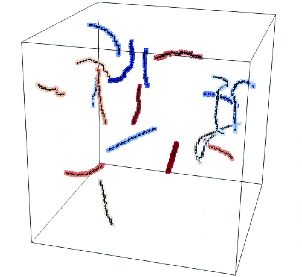
Figure 2(a) shows the IVS for a given instant for the smaller DNS used in the present work. The IVS are detected by iso-surfaces of vorticity magnitude, corresponding to the points with the
 $1\, \%$
strongest vorticity magnitude. The figure also shows the axis of the individual IVS detected by the wormtracker. Notice that there are some iso-surfaces where
$1\, \%$
strongest vorticity magnitude. The figure also shows the axis of the individual IVS detected by the wormtracker. Notice that there are some iso-surfaces where
 $\omega \gt \omega _{tr}$
that have no visible axis since IVS with fewer than 20 axis points are discarded from the statistical sample. Figure 2(b) shows the same structures (same instant) covered by the clouds of the auxiliary scalar field.
$\omega \gt \omega _{tr}$
that have no visible axis since IVS with fewer than 20 axis points are discarded from the statistical sample. Figure 2(b) shows the same structures (same instant) covered by the clouds of the auxiliary scalar field.

Figure 2. (a) Iso-surfaces of vorticity magnitude, corresponding to the points with the
 $1\, \%$
strongest vorticity magnitude (grey), together with the associated axes of the IVS. (b) Axes of the IVS as in (a), combined with the cloud of the scalar field used to link separate instants in the simulation. Both (a) and (b) correspond to the same time instant for the DNS of
$1\, \%$
strongest vorticity magnitude (grey), together with the associated axes of the IVS. (b) Axes of the IVS as in (a), combined with the cloud of the scalar field used to link separate instants in the simulation. Both (a) and (b) correspond to the same time instant for the DNS of
 $Re_{\lambda }=54$
.
$Re_{\lambda }=54$
.
The procedure outlined above allows us to obtain spatial recognition of the positions of the structures in subsequent time steps. Nevertheless, we still need to build some criteria to make comparisons between consecutive time steps. We start by defining the overlap operator
 $O_{ij}$
, which represents (in
$O_{ij}$
, which represents (in
 $\%$
) for a given scalar cloud
$\%$
) for a given scalar cloud
 $i$
how much of a worm
$i$
how much of a worm
 $j$
belongs to it (where only the points belonging to some cloud are taken into account). For instance, consider a given worm
$j$
belongs to it (where only the points belonging to some cloud are taken into account). For instance, consider a given worm
 $j$
that has
$j$
that has
 $n$
points along its filament, and suppose that from these
$n$
points along its filament, and suppose that from these
 $n$
axis points, a number
$n$
axis points, a number
 $x$
belong to cloud
$x$
belong to cloud
 $a$
,
$a$
,
 $y$
belong to cloud
$y$
belong to cloud
 $b$
, and
$b$
, and
 $z$
points do not overlap with any other existing cloud (
$z$
points do not overlap with any other existing cloud (
 $n = x + y + z$
). In this case, the matrix elements of the overlap operators
$n = x + y + z$
). In this case, the matrix elements of the overlap operators
 $O_{aj}$
and
$O_{aj}$
and
 $O_{bj}$
are defined by
$O_{bj}$
are defined by
 $O_{aj}=x/(n-z)$
and
$O_{aj}=x/(n-z)$
and
 $O_{bj}=y/(n-z)$
, respectively. We then define complete superposition when
$O_{bj}=y/(n-z)$
, respectively. We then define complete superposition when
 $O_{ij}\gt 90\, \%$
, and incomplete superposition if
$O_{ij}\gt 90\, \%$
, and incomplete superposition if
 $10 \, \%\leqslant O_{ij} \leqslant 90\, \%$
, where by superposition we mean that worm
$10 \, \%\leqslant O_{ij} \leqslant 90\, \%$
, where by superposition we mean that worm
 $j$
is overlapping cloud
$j$
is overlapping cloud
 $i$
.
$i$
.
Using these definitions and metrics, we can now look for the most simple events in the temporal evolution of a worm, namely: (i) same worm, (ii) pure splitting, (iii) pure merging, (iv) death, and (v) birth. Same worm events occur whenever there is a complete superposition of a cloud by one structure, implying the the continuation of the life of the worm. A pure splitting means that a cloud has more than one structure with complete superpositions. A pure merging happens when more than one cloud merges into one structure with incomplete superpositions on them, and at the same time, all the clouds involved must satisfy the same merging criteria. A death is detected if one cloud does not have any structure overlapping. Finally, a birth occurs because a structure is not overlapping any existing cloud. These criteria are summarised in table 3.
Table 3. Classification criteria based on the number of structures contributing to a specific range of values of the overlap operator
 $O_{ij}$
. This table should be interpreted with respect to each one of the existing clouds
$O_{ij}$
. This table should be interpreted with respect to each one of the existing clouds
 $i$
. Note that a cloud with given merging criteria will be considered as merged only if all the involved clouds satisfy the same criteria.
$i$
. Note that a cloud with given merging criteria will be considered as merged only if all the involved clouds satisfy the same criteria.

It is important to stress that, as mentioned above, the above connectivity algorithm allows one to build a global worm index from the local indexes obtained for each time step/instant of the simulation. With this procedure, all statistics taken at each instant of time can be traced back to each specific individual structure, as a time-evolving entity. The most basic entity arising from the connectivity algorithm is the lifetime map, which is shown in figure 3 for the simulation of
 $Re_{\lambda }=54$
(the other simulations result in similar maps). Figure 3(a) displays the full lifetime map for this simulation, which comprises a total of
$Re_{\lambda }=54$
(the other simulations result in similar maps). Figure 3(a) displays the full lifetime map for this simulation, which comprises a total of
 $1400$
time steps, showing the history of several worms. In this map, every horizontal line represents a worm that is ‘alive’ at some time interval, and the vertical axis is the global index/number assigned to each structure, while the horizontal axis represents the elapsed time in time step units. Note that the present analysis starts from the statistically stationary state, which explains the existence of approximately
$1400$
time steps, showing the history of several worms. In this map, every horizontal line represents a worm that is ‘alive’ at some time interval, and the vertical axis is the global index/number assigned to each structure, while the horizontal axis represents the elapsed time in time step units. Note that the present analysis starts from the statistically stationary state, which explains the existence of approximately
 $20$
worms already ‘present’ at
$20$
worms already ‘present’ at
 $\triangle t = 0$
. Figure 3(b) shows a zoom of the same map illustrating merging and splitting events. The red lines represent one structure splitting into two new structures, while the green lines show a merging of two structures into a single new structure. Note that a new global index is assigned for each new branch arising from the structures that have split or merged.
$\triangle t = 0$
. Figure 3(b) shows a zoom of the same map illustrating merging and splitting events. The red lines represent one structure splitting into two new structures, while the green lines show a merging of two structures into a single new structure. Note that a new global index is assigned for each new branch arising from the structures that have split or merged.

Figure 3. (a) Lifetime map for the simulation of
 $Re_{\lambda }=54$
. Every horizontal line represents a worm that is ‘alive’. The vertical axis shows the global index/number assigned to each structure, while the horizontal axis represents the elapsed time in time step units. The red lines show the connections among branches arising from splitting events, while the green lines show merging events. (b) Zoom of (a) highlighting one merging event from two structures into a single structure (green), and a split from one structure into two new structures (red).
$Re_{\lambda }=54$
. Every horizontal line represents a worm that is ‘alive’. The vertical axis shows the global index/number assigned to each structure, while the horizontal axis represents the elapsed time in time step units. The red lines show the connections among branches arising from splitting events, while the green lines show merging events. (b) Zoom of (a) highlighting one merging event from two structures into a single structure (green), and a split from one structure into two new structures (red).
The first detected splitting event for this simulation is shown in figure 4, in exactly the two (contiguous) times when that event was recorded. There we can see (figure 4 a) that before splitting, a filament exists with the corresponding cloud. In the very next instant (figure 4 b), we see two different structures instead. The connection is made by comparing those two structures with the cloud presented in figure 4(a). By the end of the second time step, the scalar variable with the new cloud information is reconstructed to allow the continuation of the analysis in the next time step.

Figure 4. (a) Zoom of the domain from the simulation of
 $Re_{\lambda }=54$
, showing the first splitting for the simulation with (a) the structure undergoing that splitting, and (b) the resulting branches. Note that in (a), the single cloud is also shown for the respective filament. That cloud is compared with the positions occupied by the two structures appearing in (b), thus identifying this chain of events. In (b), we now see two clouds, one surrounding each new filament (identified by different colours). The process of cloud reconstruction takes place at the end of each snapshot analysis for further time tracking.
$Re_{\lambda }=54$
, showing the first splitting for the simulation with (a) the structure undergoing that splitting, and (b) the resulting branches. Note that in (a), the single cloud is also shown for the respective filament. That cloud is compared with the positions occupied by the two structures appearing in (b), thus identifying this chain of events. In (b), we now see two clouds, one surrounding each new filament (identified by different colours). The process of cloud reconstruction takes place at the end of each snapshot analysis for further time tracking.
4. Results
In this section, we use the temporal vortex tracking algorithm described above to (i) compute the mean lifetime of the IVS, (ii) estimate the population of the IVS present in a given simulation and (iii) study the history of the IVS in terms of their events, such as splits and merging.
4.1. Study of the survival function of the IVS
We start the discussion of the results with the investigation of the mean lifetimes of the IVS. In this process, we make the following assumption: branches arising from splitting or merging events are considered as individual IVS for the purpose of time tracking the IVS. Thus the background dynamics of the IVS, and possible interactions with other IVS, are not taken into consideration when analysing the lifetime statistics. In § 4.4 it will be shown that splits and mergers have a negligible effect on the observed lifetime.
The analysis is based on the concept of the survival function (SF) denoted as
 $S(\tau )$
, which is used to estimate lifetimes in different areas of science, medicine and engineering (Klein & Moeschberger Reference Klein and Moeschberger2003). If the lifetime of a structure (
$S(\tau )$
, which is used to estimate lifetimes in different areas of science, medicine and engineering (Klein & Moeschberger Reference Klein and Moeschberger2003). If the lifetime of a structure (
 $T$
) is a continuous random variable, then the SF is the probability of the structure having a lifetime bigger than time
$T$
) is a continuous random variable, then the SF is the probability of the structure having a lifetime bigger than time
 $\tau$
, i.e. the SF is defined as
$\tau$
, i.e. the SF is defined as
 \begin{equation} S(\tau ) = P(T \gt \tau ) = \int _{\tau }^{\infty } f(u)\, {\rm d}u, \end{equation}
where
 $f(\tau )$
is the probability density function (PDF) of the IVS, having a lifetime equal to
$f(\tau )$
is the probability density function (PDF) of the IVS, having a lifetime equal to
 $\tau$
. The cumulative distribution function (CDF)
$\tau$
. The cumulative distribution function (CDF)
 $F(\tau )$
is defined as the probability that the survival time is less than or equal to a specific time
$F(\tau )$
is defined as the probability that the survival time is less than or equal to a specific time
 $\tau$
:
$\tau$
:
 \begin{equation} F(\tau ) = P(T \leqslant \tau ) = \int _0^{\tau } f(u)\, {\rm d}u, \end{equation}
i.e.
 $S(\tau ) = 1 - F(\tau )$
, since
$S(\tau ) = 1 - F(\tau )$
, since
 $\int _0^{\infty } f(u)\, {\rm d}u = 1$
. We measure the lifetime of each structure by subtracting its death time (when we can no longer follow the structure) from its birth time (when we start detecting it).
$\int _0^{\infty } f(u)\, {\rm d}u = 1$
. We measure the lifetime of each structure by subtracting its death time (when we can no longer follow the structure) from its birth time (when we start detecting it).
In the present work, all the lifetime analysis is based on the Kaplan–Meier (KM) estimator (Kaplan & Meier Reference Kaplan and Meier1958), which is a non-parametric method used to obtain the SF and to estimate lifetimes in different areas of science, medicine and engineering (Kaplan & Meier Reference Kaplan and Meier1958).
The KM estimator for the SF, denoted by
 $\hat {S}(\tau )$
, takes the following form when applied to the study of the lifetimes of the IVS:
$\hat {S}(\tau )$
, takes the following form when applied to the study of the lifetimes of the IVS:
 \begin{equation} \hat {S} ( \tau ) =\left \{ \begin{array}{ll} 1 , & \tau \lt \tau _{1}, \\ \displaystyle\prod _{\tau _{i}\leqslant \tau }\left [1-\dfrac {d_{i}}{r_{i}}\right ] , & \tau \geqslant \tau _{1}, \end{array} \right . \end{equation}
where
 $\tau _1$
is the smallest recorded lifetime, the
$\tau _1$
is the smallest recorded lifetime, the
 $\tau _{i}$
form an ordered list containing the lifetimes of all tracked IVS, where
$\tau _{i}$
form an ordered list containing the lifetimes of all tracked IVS, where
 $\tau _i$
is increasing with
$\tau _i$
is increasing with
 $i$
,
$i$
,
 $d_{i}$
is the number of structures that died at lifetime
$d_{i}$
is the number of structures that died at lifetime
 $\tau _{i}$
, and
$\tau _{i}$
, and
 $r_{i}$
is the number of structures that are at risk of ‘dying’ at lifetime
$r_{i}$
is the number of structures that are at risk of ‘dying’ at lifetime
 $\tau _i$
(that die at lifetimes greater than or equal to
$\tau _i$
(that die at lifetimes greater than or equal to
 $\tau _{i}$
). Naturally, at time
$\tau _{i}$
). Naturally, at time
 $\tau _{1}$
, all the structures in the sample are at risk, thus
$\tau _{1}$
, all the structures in the sample are at risk, thus
 $r_{1}=N_{s}$
. The actual use of this estimator is described in some detail in an example given below.
$r_{1}=N_{s}$
. The actual use of this estimator is described in some detail in an example given below.
One big advantage of this estimator is that it allows one to use all the existing samples of IVS lifetimes. Recall that when the time tracking of the IVS is started (corresponding to time
 $t=0$
), some of the IVS are already alive, and by the end of the simulated time, some IVS that will ‘die’ later are still alive. It follows that if these structures are considered in a ‘classical’ procedure to estimate the mean lifetime of the IVS, then the resulting estimated mean lifetime will be smaller than or equal to the ‘real’ one. The KM estimator allows one to use all the available data to obtain the SF without incurring this problem. Formally, this means that these IVS (from the start and end of the simulated time) are treated as right-censored data, while all the other IVS lifetime measurements are considered as fully observed (Kaplan & Meier Reference Kaplan and Meier1958). To clarify, in the use of (4.3) with censored data, censored structures are not classified as deaths. As an example, suppose that at lifetime
$t=0$
), some of the IVS are already alive, and by the end of the simulated time, some IVS that will ‘die’ later are still alive. It follows that if these structures are considered in a ‘classical’ procedure to estimate the mean lifetime of the IVS, then the resulting estimated mean lifetime will be smaller than or equal to the ‘real’ one. The KM estimator allows one to use all the available data to obtain the SF without incurring this problem. Formally, this means that these IVS (from the start and end of the simulated time) are treated as right-censored data, while all the other IVS lifetime measurements are considered as fully observed (Kaplan & Meier Reference Kaplan and Meier1958). To clarify, in the use of (4.3) with censored data, censored structures are not classified as deaths. As an example, suppose that at lifetime
 $\tau _{i}$
we have five structures (
$\tau _{i}$
we have five structures (
 $r_{i}=5$
), then one structure dies (
$r_{i}=5$
), then one structure dies (
 $d_{i}=1$
) and one is censored (
$d_{i}=1$
) and one is censored (
 $c_{i}=1$
). Then at time
$c_{i}=1$
). Then at time
 $\tau _{i+1}$
, we have
$\tau _{i+1}$
, we have
 $r_{i+1}=r_{i}-d_{i}-c_{i} = 5-1-1=3$
, where
$r_{i+1}=r_{i}-d_{i}-c_{i} = 5-1-1=3$
, where
 $c_{i}$
is the number of censored structures, which are subtracted at stage
$c_{i}$
is the number of censored structures, which are subtracted at stage
 $i$
.
$i$
.

Figure 5. Survival functions
 $\hat {S}(\tau ) = 1 - F(\tau )$
of the worms’ lifetimes obtained through (4.3), where data for lifetimes smaller than a given threshold value
$\hat {S}(\tau ) = 1 - F(\tau )$
of the worms’ lifetimes obtained through (4.3), where data for lifetimes smaller than a given threshold value
 $\tau _{0}$
have been removed (filtered), for the DNS with (a)
$\tau _{0}$
have been removed (filtered), for the DNS with (a)
 $Re_{\lambda }=54$
, (b)
$Re_{\lambda }=54$
, (b)
 $Re_{\lambda }=91$
, (c)
$Re_{\lambda }=91$
, (c)
 $Re_{\lambda }=143$
and (d)
$Re_{\lambda }=143$
and (d)
 $Re_{\lambda }=189$
. (The DNS with
$Re_{\lambda }=189$
. (The DNS with
 $Re_{\lambda }=239$
show similar characteristics, not shown.) Here,
$Re_{\lambda }=239$
show similar characteristics, not shown.) Here,
 $\tau$
is the random variable describing the lifetime, and
$\tau$
is the random variable describing the lifetime, and
 $\tau _{\eta }$
is the Kolmogorov time scale. In the SF for
$\tau _{\eta }$
is the Kolmogorov time scale. In the SF for
 $\tau _{0}/\tau _{\eta } = 0$
, all the lifetimes have been used, whereas in the other curves, lifetimes smaller than
$\tau _{0}/\tau _{\eta } = 0$
, all the lifetimes have been used, whereas in the other curves, lifetimes smaller than
 $\tau _{0}/\tau _{\eta } = 0.1, 0.2, 0.5, 1$
have been eliminated from the statistical sample.
$\tau _{0}/\tau _{\eta } = 0.1, 0.2, 0.5, 1$
have been eliminated from the statistical sample.
The next two figures (figures 5 and 6) show the estimated SFs obtained by applying (4.3) to the lifetime data originated from all the DNS used in the present work,
 $\hat {S}(\tau ) = 1 - \hat {F}(\tau ) = 1 - \hat {P} (T/\tau _{\eta }\lt \tau /\tau _{\eta } )$
, where
$\hat {S}(\tau ) = 1 - \hat {F}(\tau ) = 1 - \hat {P} (T/\tau _{\eta }\lt \tau /\tau _{\eta } )$
, where
 $\hat {P}(T \leqslant \tau )$
is the estimated CDF. As expected, all the SFs decrease as the lifetime increases. Interestingly, all the SFs are well approximated by an exponential function, provided that the number of available samples is sufficiently high. Appendix A compares the SF obtained with the KM estimator to that obtained using a ‘classical’ (straightforward) approach demonstrating the advantages of the former.
$\hat {P}(T \leqslant \tau )$
is the estimated CDF. As expected, all the SFs decrease as the lifetime increases. Interestingly, all the SFs are well approximated by an exponential function, provided that the number of available samples is sufficiently high. Appendix A compares the SF obtained with the KM estimator to that obtained using a ‘classical’ (straightforward) approach demonstrating the advantages of the former.
The mean lifetime of the IVS is simply the integrated SF; however, we need to address two issues, to which we now turn our attention before carrying out this integration. First, we need to address the effect of some of the thresholds used in the temporal time tracking procedure. One of these is the threshold value of the considered time itself,
 $\tau$
. It is plausible that data obtained for extremely small times will be ‘polluted’ by numerical artefacts, such as, for instance, when IVS oscillate very close to the detected threshold and can ‘appear’ and ‘disappear’ from the data for very small simulated times. We believe that this and similar non-physical behaviours are essentially present when too small lifetimes are considered. For that reason, we study how sensitive the lifetime distributions are to small times by eliminating them from the data, i.e. to when low time scale cut-offs are used. In short, we argue that representative IVS should live more than a certain time
$\tau$
. It is plausible that data obtained for extremely small times will be ‘polluted’ by numerical artefacts, such as, for instance, when IVS oscillate very close to the detected threshold and can ‘appear’ and ‘disappear’ from the data for very small simulated times. We believe that this and similar non-physical behaviours are essentially present when too small lifetimes are considered. For that reason, we study how sensitive the lifetime distributions are to small times by eliminating them from the data, i.e. to when low time scale cut-offs are used. In short, we argue that representative IVS should live more than a certain time
 $\tau _{0}$
, and we investigate this effect by recomputing the CDF for our data by eliminating structures living less than a given time
$\tau _{0}$
, and we investigate this effect by recomputing the CDF for our data by eliminating structures living less than a given time
 $\tau _{0}$
.
$\tau _{0}$
.

Figure 6. Survival functions
 $\hat {S}(\tau ) = 1 - F(\tau )$
of the worms’ lifetimes obtained through (4.3), with different final simulated times
$\hat {S}(\tau ) = 1 - F(\tau )$
of the worms’ lifetimes obtained through (4.3), with different final simulated times
 $t_{f}$
, for the DNS with (a)
$t_{f}$
, for the DNS with (a)
 $Re_{\lambda }=54$
, (b)
$Re_{\lambda }=54$
, (b)
 $Re_{\lambda }=91$
, (c)
$Re_{\lambda }=91$
, (c)
 $Re_{\lambda }=143$
and (d)
$Re_{\lambda }=143$
and (d)
 $Re_{\lambda }=189$
. (The DNS with
$Re_{\lambda }=189$
. (The DNS with
 $Re_{\lambda }=239$
show similar characteristics, not shown.) In these curves, times smaller than
$Re_{\lambda }=239$
show similar characteristics, not shown.) In these curves, times smaller than
 $\tau _{0} = 0.5 \tau _{\eta }$
have been removed (filtered) following the discussion in figure 5. Here,
$\tau _{0} = 0.5 \tau _{\eta }$
have been removed (filtered) following the discussion in figure 5. Here,
 $\tau$
is the random variable describing the lifetime, and
$\tau$
is the random variable describing the lifetime, and
 $\tau _L$
is the integral time scale (
$\tau _L$
is the integral time scale (
 $\tau _{\eta }$
is the Kolmogorov time scale).
$\tau _{\eta }$
is the Kolmogorov time scale).
Figure 5 shows the effect of
 $\tau _0$
on the SFs for
$\tau _0$
on the SFs for
 $\tau _0$
in the range
$\tau _0$
in the range
 $ 0 \leqslant \tau _{0}/\tau _{\eta } \leqslant 1$
. In the SF for
$ 0 \leqslant \tau _{0}/\tau _{\eta } \leqslant 1$
. In the SF for
 $\tau _{0}/\tau _{\eta } = 0$
, no removal was done, i.e. all the lifetimes have been used. The figure shows that using different cut-offs
$\tau _{0}/\tau _{\eta } = 0$
, no removal was done, i.e. all the lifetimes have been used. The figure shows that using different cut-offs
 $\tau _{0}/\tau _{\eta }$
affects the SF shape; however, for each simulation, the SF converges to virtually the same function for
$\tau _{0}/\tau _{\eta }$
affects the SF shape; however, for each simulation, the SF converges to virtually the same function for
 $\tau _{0} \geqslant 0.5 \tau _{\eta }$
. For example, there is virtually no diference between the SFs for the DNS of
$\tau _{0} \geqslant 0.5 \tau _{\eta }$
. For example, there is virtually no diference between the SFs for the DNS of
 $Re_{\lambda }=143$
(figure 6
c) corresponding to
$Re_{\lambda }=143$
(figure 6
c) corresponding to
 $\tau _{0}/\tau _{\eta } = 0.5$
and
$\tau _{0}/\tau _{\eta } = 0.5$
and
 $\tau _{0}/\tau _{\eta } = 1$
. Similar results are observed for the other cases. We therefore proceed with our analysis by eliminating all the structures displaying lifetimes smaller than
$\tau _{0}/\tau _{\eta } = 1$
. Similar results are observed for the other cases. We therefore proceed with our analysis by eliminating all the structures displaying lifetimes smaller than
 $\tau _{0}/\tau _{\eta }=0.5$
, as it is likely that events lasting less than half a Kolmogorov time are affected by artificial numerical ‘noise’ described above.
$\tau _{0}/\tau _{\eta }=0.5$
, as it is likely that events lasting less than half a Kolmogorov time are affected by artificial numerical ‘noise’ described above.
The second variable that one needs to investigate is the total time duration of the simulations,
 $t_f$
. In order to investigate the effect of this variable in the results obtained, we fix
$t_f$
. In order to investigate the effect of this variable in the results obtained, we fix
 $\tau _{0}/\tau _{\eta }=0.5$
and repeat the SF estimation for different simulation times
$\tau _{0}/\tau _{\eta }=0.5$
and repeat the SF estimation for different simulation times
 $t_{f}$
. Figure 6 shows the resulting SF for all the simulations carried out in this work, which can be seen as temporal evolutions of this estimation. It is clear that as the final simulated time increases, the SFs converge into the same curve (for each simulation), with an approximately constant slope, where the tail of the SF extends to longer times as
$t_{f}$
. Figure 6 shows the resulting SF for all the simulations carried out in this work, which can be seen as temporal evolutions of this estimation. It is clear that as the final simulated time increases, the SFs converge into the same curve (for each simulation), with an approximately constant slope, where the tail of the SF extends to longer times as
 $t_{f}$
increases. An implication of this observation is that very-long-living structures are relatively rare and are ‘seen’ only for sufficiently large time windows. Also, for each case, there is virtually no difference between the SFs obtained for the two biggest simulated times. For instance, for the DNS of
$t_{f}$
increases. An implication of this observation is that very-long-living structures are relatively rare and are ‘seen’ only for sufficiently large time windows. Also, for each case, there is virtually no difference between the SFs obtained for the two biggest simulated times. For instance, for the DNS of
 $Re_{\lambda }=143$
(figure 6
c) , the curves corresponding to
$Re_{\lambda }=143$
(figure 6
c) , the curves corresponding to
 $t_{f}/\tau _L = 5.8$
and
$t_{f}/\tau _L = 5.8$
and
 $7.4$
, are virtually the same. This shows that the total (final) simulated time (
$7.4$
, are virtually the same. This shows that the total (final) simulated time (
 $t_f/\tau _L \approx 6$
–
$t_f/\tau _L \approx 6$
–
 $7$
) is sufficient to capture the details of the SF for each case.
$7$
) is sufficient to capture the details of the SF for each case.
Following the results from the above discussion, we now proceed with the estimation of the mean lifetimes of the IVS by using the appropriate data for each simulation, i.e. we will be using the data from the green curves from figures 6(a–d), which comprise the entire simulated times for the DNS,
 $t_f/\tau _L \approx 6$
–
$t_f/\tau _L \approx 6$
–
 $7$
, and by eliminating events (lifetimes) lasting less than
$7$
, and by eliminating events (lifetimes) lasting less than
 $\tau _{0}/\tau _{\eta }=0.5$
.
$\tau _{0}/\tau _{\eta }=0.5$
.
4.2. Computing the characteristic lifetime of the IVS
Having now determined what data can be used to compute the SF (using only IVS with lifetimes greater that
 $\tau _{0}/\tau _{\eta }=0.5$
) and that the total simulated time is sufficient to accurately compute these functions in each case, we now use three different methods to compute the characteristic lifetime of a structure, which we denote by
$\tau _{0}/\tau _{\eta }=0.5$
) and that the total simulated time is sufficient to accurately compute these functions in each case, we now use three different methods to compute the characteristic lifetime of a structure, which we denote by
 $\tau _{ivs}$
. We will see that the three methods lead to similar values of the characteristic lifetime, and that the results allow us to establish the scaling laws associated with this quantity. In any case, whatever the method used to estimate the SF, it is important to stress that the mean lifetime is always given by the integration of the SF, i.e. for a continuous SF (
$\tau _{ivs}$
. We will see that the three methods lead to similar values of the characteristic lifetime, and that the results allow us to establish the scaling laws associated with this quantity. In any case, whatever the method used to estimate the SF, it is important to stress that the mean lifetime is always given by the integration of the SF, i.e. for a continuous SF (
 $S(\tau )$
), we have
$S(\tau )$
), we have
 \begin{equation} \tau _{ivs} = \int _0^{\infty } S(\tau )\, {\rm d}\tau = \int _0^{\infty } \tau\, f(\tau )\, {\rm d}\tau , \end{equation}
where the second equality stems from the definition of the SF in (4.1).
Formally, the restriction on
 $\tau _0$
discussed above means that the PDF
$\tau _0$
discussed above means that the PDF
 $f ( \tau )$
for the lifetime is defined as
$f ( \tau )$
for the lifetime is defined as
 \begin{equation} f ( \tau ) =\left \{ \begin{array}{ll} 0 , & 0\leqslant \tau \lt \tau _{0}, \\ h ( \tau ) , & \tau \geqslant \tau _{0}, \end{array} \right . \end{equation}
where
 $h ( \tau )$
is a restricted PDF (whose CDF is
$h ( \tau )$
is a restricted PDF (whose CDF is
 $F(\tau ) = \int _{\tau _0}^{\tau } h(t')\, {\rm d} t'$
), while the SF now becomes
$F(\tau ) = \int _{\tau _0}^{\tau } h(t')\, {\rm d} t'$
), while the SF now becomes
 \begin{equation} S ( \tau ) =\left \{ \begin{array}{ll} 1 , & 0\leqslant \tau \lt \tau _{0}, \\ 1-\displaystyle\int _{\tau _{0}}^{\tau }h(t^{\prime })\,{\rm d}t^{\prime } , & \tau \geqslant \tau _{0}, \end{array} \right . \end{equation}
since the CDF and the SF are defined by
 $P (T/\tau _{\eta }\lt \tau /\tau _{\eta } )$
and
$P (T/\tau _{\eta }\lt \tau /\tau _{\eta } )$
and
 $S ( \tau )=1-P (T/\tau _{\eta }\lt \tau /\tau _{\eta } )$
, respectively, as before.
$S ( \tau )=1-P (T/\tau _{\eta }\lt \tau /\tau _{\eta } )$
, respectively, as before.
With these definitions, the mean lifetime of the IVS can now be estimated by
 \begin{equation} \tau _{ivs} = \int _{0}^{\infty } S ( \tau )\, {\rm d} \tau = \tau _{0}+\int _{\tau _{0}}^{\infty }\left [1-\int _{\tau _{0}}^{\tau }h (t^{\prime })\,{\rm d}t^{\prime }\right ]{\rm d}\tau . \end{equation}
Notice that in figures 5(a–d), the displayed functions are precisely
 $1 - P (T/\tau _{\eta }\lt \tau /\tau _{\eta } ) = 1-\int _{\tau _{0}}^{\tau }h (t^{\prime } )\,{\rm d}t$
, and the horizontal axis represents the shifted time
$1 - P (T/\tau _{\eta }\lt \tau /\tau _{\eta } ) = 1-\int _{\tau _{0}}^{\tau }h (t^{\prime } )\,{\rm d}t$
, and the horizontal axis represents the shifted time
 $ (\tau - \tau _{0} )$
, which means that the integral in (4.7) is simply the area enclosed by the SFs.
$ (\tau - \tau _{0} )$
, which means that the integral in (4.7) is simply the area enclosed by the SFs.
As remarked above, a careful analysis of figures 5 and 6 suggests that the SFs are well approximated by an exponential function for
 $\tau \geqslant \tau _0$
:
$\tau \geqslant \tau _0$
:
 \begin{equation} \hat {S}(\tau ) = 1 - \hat {P}(T/\tau _{\eta } \lt \tau /\tau _{\eta }) \approx {\rm e}^{ - ( \tau - \tau _{0} )/\zeta }, \end{equation}
where
 $\zeta$
is the inverse of the decay rate associated with the SF, or the mean lifetime of the IVS (
$\zeta$
is the inverse of the decay rate associated with the SF, or the mean lifetime of the IVS (
 $\tau _{ivs}$
). The use of an exponential function greatly simplifies the computation of the mean lifetime of the IVS, which is simply
$\tau _{ivs}$
). The use of an exponential function greatly simplifies the computation of the mean lifetime of the IVS, which is simply
 \begin{equation} \tau _{ivs} = \tau _0 + \int _{\tau _0}^{\infty } {\rm e}^{ - ( \tau - \tau _{0})/\zeta }\, {\rm d}\tau = \tau _0 + \zeta , \end{equation}
if one considers an infinite time of recorded events.
The first (straightforward) method to estimate the mean lifetime of the IVS consists on using the so-called restricted mean survival time (RMST) (Royston & Parmar Reference Royston and Parmar2013), whereby the SF is integrated up to a specific time point
 $\tau _{{max}}$
:
$\tau _{{max}}$
:
 \begin{equation} \tau _{ivs}^{RMST} = \tau _0 + \int _{\tau _0}^{\tau _{{max}}} \hat {S} ( \tau )\, {\rm d} \tau , \end{equation}
where
 $\hat {S} ( \tau )$
represents the estimated SF, and
$\hat {S} ( \tau )$
represents the estimated SF, and
 $\tau _{{max}}$
is the measured lifetime for the longest-lived structure. Specifically, this value was assigned to
$\tau _{{max}}$
is the measured lifetime for the longest-lived structure. Specifically, this value was assigned to
 $(\tau _{{max}} - \tau _0) / \tau _{\eta } = 21.74, 22.52, 38.16, 37.01$
for the DNS with
$(\tau _{{max}} - \tau _0) / \tau _{\eta } = 21.74, 22.52, 38.16, 37.01$
for the DNS with
 $Re_{\lambda }=54, 91, 143, 189$
, respectively. Using this approach, the mean lifetime of the IVS is simply given by (4.10), where the integration is performed until the longest detected time
$Re_{\lambda }=54, 91, 143, 189$
, respectively. Using this approach, the mean lifetime of the IVS is simply given by (4.10), where the integration is performed until the longest detected time
 $\tau _{{max}}$
for each one of the simulations used here.
$\tau _{{max}}$
for each one of the simulations used here.
A second method to estimate the mean lifetime of the IVS consists in using the maximum likelihood estimator (MLE) (Klein & Moeschberger Reference Klein and Moeschberger2003). In this case, and again by assuming that the SF is described by an exponential function (4.8), the parameter
 $\zeta$
can be estimated by maximising the probability to obtain the existing/available data. Formally, for right-censored data, the so-called likelihood function for the parameter
$\zeta$
can be estimated by maximising the probability to obtain the existing/available data. Formally, for right-censored data, the so-called likelihood function for the parameter
 $\zeta$
is given by
$\zeta$
is given by
 \begin{equation} L (\zeta )=\prod _{i} f ( \tau _{i})\prod _{n} S ( \tau _{n}) , \end{equation}
where
 $S ( \tau )=\exp [- ( \tau - \tau _{0} )/\zeta ]$
is again the SF defined by the parameter
$S ( \tau )=\exp [- ( \tau - \tau _{0} )/\zeta ]$
is again the SF defined by the parameter
 $\zeta$
, and
$\zeta$
, and
 $f ( \tau ) = \exp [- ( \tau - \tau _{0} )/\zeta ]/\zeta$
is the PDF of the IVS lifetimes, also assumed to follow an exponential distribution, consistently with the assumed form of the SF (and with the observed shape of the PDF shown in Appendix A). Notice that in (4.11), the
$f ( \tau ) = \exp [- ( \tau - \tau _{0} )/\zeta ]/\zeta$
is the PDF of the IVS lifetimes, also assumed to follow an exponential distribution, consistently with the assumed form of the SF (and with the observed shape of the PDF shown in Appendix A). Notice that in (4.11), the
 $i$
index runs for all fully observed data, whereas the
$i$
index runs for all fully observed data, whereas the
 $n$
index runs for all right-censored data. With the value of
$n$
index runs for all right-censored data. With the value of
 $\zeta$
obtained in this way, the mean lifetime of the ‘worms’ using this estimator is
$\zeta$
obtained in this way, the mean lifetime of the ‘worms’ using this estimator is
 $\tau _{ivs}^{{MLE}} = \tau _0 + \zeta$
.
$\tau _{ivs}^{{MLE}} = \tau _0 + \zeta$
.
Finally, the third method (Fit) consists in assuming that the SF obtained for the simulations represented in figures 6(a) and 6(d) is defined by an exponential function, and obtaining the parameter for each curve, namely
 $\zeta$
, by using the least squares regression line. As in the other methods, the mean lifetime of the IVS is simply
$\zeta$
, by using the least squares regression line. As in the other methods, the mean lifetime of the IVS is simply
 $\tau _{ivs}^{Fit} = \tau _0 + \zeta$
.
$\tau _{ivs}^{Fit} = \tau _0 + \zeta$
.
Table 4 displays the mean lifetime of the IVS (
 $\tau _{ivs}$
) obtained by employing the three methods described above. The mean lifetimes are normalised with the Kolmogorov time (
$\tau _{ivs}$
) obtained by employing the three methods described above. The mean lifetimes are normalised with the Kolmogorov time (
 $\tau _{\eta }$
) and with the integral time scale (
$\tau _{\eta }$
) and with the integral time scale (
 $\tau _L$
). It is reassuring to see that the three different methods lead to very similar mean lifetime values for all DNS data.
$\tau _L$
). It is reassuring to see that the three different methods lead to very similar mean lifetime values for all DNS data.
Table 4. Mean lifetimes of the IVS estimated with three different methods, normalised by the Kolmogorov time
 $\tau _{\eta }$
and by the integral time scale
$\tau _{\eta }$
and by the integral time scale
 $\tau _{L}$
, for all the DNS used in the present work: number of collocation points (
$\tau _{L}$
, for all the DNS used in the present work: number of collocation points (
 $N^3$
); Taylor-microscale-based Reynolds number (
$N^3$
); Taylor-microscale-based Reynolds number (
 $Re_{\lambda }$
); mean lifetime using the restricted mean survival time (
$Re_{\lambda }$
); mean lifetime using the restricted mean survival time (
 $\tau _{ivs}^{{RMST}}$
); mean lifetime using the maximum likelihood estimator considering an exponential distribution (
$\tau _{ivs}^{{RMST}}$
); mean lifetime using the maximum likelihood estimator considering an exponential distribution (
 $\tau _{ivs}^{{MLE}}$
); mean lifetime measured by fitting the KM estimate for the SF (
$\tau _{ivs}^{{MLE}}$
); mean lifetime measured by fitting the KM estimate for the SF (
 $\tau _{ivs}^{{Fit}}$
). The last row corresponds to the DNS where the forcing is centred at
$\tau _{ivs}^{{Fit}}$
). The last row corresponds to the DNS where the forcing is centred at
 $k_p = 4$
(instead of
$k_p = 4$
(instead of
 $k_p=2$
).
$k_p=2$
).

The mean lifetime is typically equal to
 $\tau _{ivs} / \tau _{\eta } \approx 3$
–
$\tau _{ivs} / \tau _{\eta } \approx 3$
–
 $4$
and
$4$
and
 $\tau _{ivs} / \tau _{L} \approx 0.1$
–
$\tau _{ivs} / \tau _{L} \approx 0.1$
–
 $0.3$
. This is much smaller than the integral time scale usually claimed as being the typical lifetime of the IVS. Our explanation, supported in several animations, is that even though many of these long lifetime structures do exist, as inferred from the SFs in figures 6(a–d), they represent extreme lifetime events, which are relatively rare, even if probably these are the structures that we retain in our mind from movies and visualisations. Indeed, from figures 6(a–d), one can see that some IVS have lives that are much longer than the mean, with recorded lifetime events
$0.3$
. This is much smaller than the integral time scale usually claimed as being the typical lifetime of the IVS. Our explanation, supported in several animations, is that even though many of these long lifetime structures do exist, as inferred from the SFs in figures 6(a–d), they represent extreme lifetime events, which are relatively rare, even if probably these are the structures that we retain in our mind from movies and visualisations. Indeed, from figures 6(a–d), one can see that some IVS have lives that are much longer than the mean, with recorded lifetime events
 $\approx 15 \tau _{\eta }$
,
$\approx 15 \tau _{\eta }$
,
 $\approx 22 \tau _{\eta }$
,
$\approx 22 \tau _{\eta }$
,
 $\approx 35 \tau _{\eta }$
and
$\approx 35 \tau _{\eta }$
and
 $\approx 38 \tau _{\eta }$
for the DNS with
$\approx 38 \tau _{\eta }$
for the DNS with
 $Re_{\lambda }=54, 91, 143$
and
$Re_{\lambda }=54, 91, 143$
and
 $189$
, respectively. From table 1, one can see that these extreme lifetimes correspond to
$189$
, respectively. From table 1, one can see that these extreme lifetimes correspond to
 $\approx 1.8 \tau _L$
,
$\approx 1.8 \tau _L$
,
 $\approx 1.9 \tau _L$
,
$\approx 1.9 \tau _L$
,
 $\approx 2.0 \tau _L$
and
$\approx 2.0 \tau _L$
and
 $\approx 1.6 \tau _L$
, respectively. This suggests that the extremes scale with the integral time scale
$\approx 1.6 \tau _L$
, respectively. This suggests that the extremes scale with the integral time scale
 $\tau _L$
, but not the mean.
$\tau _L$
, but not the mean.
Biferale et al. (Reference Biferale, Scagliarini and Toschi2010) also observed extreme lifetime events of the order of the integral time scale; however, their computed mean values were
 $\tau _{ivs} /\tau _{\eta } \approx 17$
and
$\tau _{ivs} /\tau _{\eta } \approx 17$
and
 $25$
for DNS with
$25$
for DNS with
 $Re_{\lambda }=65$
and
$Re_{\lambda }=65$
and
 $180$
, respectively, which is 3–5 times higher than our values, and reveals an opposite trend with the Reynolds number. The difference can be attributed to the indirect procedure used in that work, which involved the clustering of light particles inside the vortex cores. As recognised in that paper, particle clustering requires persistent vortices, since the particles need time to move into the vortex cores. Hence their detection method may favour long-lived structures. Also, the analysis of lifetimes from particles trapped inside the IVS does exclude situations of IVS merging or splitting that are differentiated in the present study. Another difference is the chosen magnitude of the threshold used to detect the IVS. Moreover, it is unclear how the small sample size used in that work might have affected their result, and whether care was taken to exclude lives from the start and end of the simulations. Arguably, the present tracking method is the first rigorous attempt at investigating this problem because of the method being ‘direct’ (the IVS are tracked in time, not their effects) and the number of samples is very large.
$180$
, respectively, which is 3–5 times higher than our values, and reveals an opposite trend with the Reynolds number. The difference can be attributed to the indirect procedure used in that work, which involved the clustering of light particles inside the vortex cores. As recognised in that paper, particle clustering requires persistent vortices, since the particles need time to move into the vortex cores. Hence their detection method may favour long-lived structures. Also, the analysis of lifetimes from particles trapped inside the IVS does exclude situations of IVS merging or splitting that are differentiated in the present study. Another difference is the chosen magnitude of the threshold used to detect the IVS. Moreover, it is unclear how the small sample size used in that work might have affected their result, and whether care was taken to exclude lives from the start and end of the simulations. Arguably, the present tracking method is the first rigorous attempt at investigating this problem because of the method being ‘direct’ (the IVS are tracked in time, not their effects) and the number of samples is very large.
Finally, from table 4 it is clear that the lifetime values show a decreasing trend with the increase of the Reynolds number, i.e. the available data suggest that the mean lifetime of the IVS at high Reynolds numbers does not scale with either
 $\tau _{\eta }$
or
$\tau _{\eta }$
or
 $\tau _L$
.
$\tau _L$
.
To allow a closer look at the effects of the Reynolds number on the shapes of the SFs, figure 7 gathers all the SFs used here, for the different Reynolds numbers available in the present work. Again, we are seeing the same SF already displayed in figures 6(a–d), together with the DNS with
 $Re_{\lambda }=239$
, where only
$Re_{\lambda }=239$
, where only
 $1/8$
of the computational domain is used to time track the IVS. This does not affect the mean lifetime of the IVS for this last (bigger) DNS, but it may limit the amount of extreme events available in this simulation (see Appendix C). We can see here more clearly than before that as the Reynolds number increases, the slope of each curve – and consequently the area under the curve (which represents the mean lifetime) – decreases. This is consistent with the results shown in table 4. However, we also observe another interesting result, which is that the duration (size) of the recorded lifetimes also increases with the Reynolds number. Whereas for
$1/8$
of the computational domain is used to time track the IVS. This does not affect the mean lifetime of the IVS for this last (bigger) DNS, but it may limit the amount of extreme events available in this simulation (see Appendix C). We can see here more clearly than before that as the Reynolds number increases, the slope of each curve – and consequently the area under the curve (which represents the mean lifetime) – decreases. This is consistent with the results shown in table 4. However, we also observe another interesting result, which is that the duration (size) of the recorded lifetimes also increases with the Reynolds number. Whereas for
 $Re_{\lambda } =54$
no single recorded IVS lives longer than
$Re_{\lambda } =54$
no single recorded IVS lives longer than
 $\tau _{ivs}/\tau _{\eta } =25$
, for
$\tau _{ivs}/\tau _{\eta } =25$
, for
 $Re_{\lambda } =189$
many IVS live longer than
$Re_{\lambda } =189$
many IVS live longer than
 $\tau _{ivs}/\tau _{\eta } =35$
. Not only do the longest recorded lifetimes increase with the Reynolds number, following approximate
$\tau _{ivs}/\tau _{\eta } =35$
. Not only do the longest recorded lifetimes increase with the Reynolds number, following approximate
 $\tau _L$
scaling, but also the total ‘spectrum’ of existing lifetime events increases. This result is probably not surprising since the increase of the Reynolds number is typically associated with an increase in the multiplicity of length, velocity and time ‘events’ in turbulent flows, but it is nonetheless interesting to observe it here in the context of the analysis of the lifetimes of the IVS. (This trend is not visible in the bigger DNS probably because of the use of only
$\tau _L$
scaling, but also the total ‘spectrum’ of existing lifetime events increases. This result is probably not surprising since the increase of the Reynolds number is typically associated with an increase in the multiplicity of length, velocity and time ‘events’ in turbulent flows, but it is nonetheless interesting to observe it here in the context of the analysis of the lifetimes of the IVS. (This trend is not visible in the bigger DNS probably because of the use of only
 $1/8$
of the computational domain.)
$1/8$
of the computational domain.)

Figure 7. Comparison between the several SFs obtained for the different Reynolds numbers available in the present work. Each SF shown here is the reference SF used in the discussion of the lifetime already displayed in figures 6(a–d), together with the DNS with
 $Re_{\lambda }=239$
. Here,
$Re_{\lambda }=239$
. Here,
 $\tau$
is the random variable describing the lifetime, while
$\tau$
is the random variable describing the lifetime, while
 $\tau _{\eta }$
is the Kolmogorov time scale.
$\tau _{\eta }$
is the Kolmogorov time scale.

Figure 8. Mean lifetimes of the IVS computed with three different methods (
 $\tau _{ivs}^{{RMST}}$
,
$\tau _{ivs}^{{RMST}}$
,
 $\tau _{ivs}^{{MLE}}$
,
$\tau _{ivs}^{{MLE}}$
,
 $\tau _{ivs}^{{Fit}}$
), normalised with the Kolmogorov time scale (
$\tau _{ivs}^{{Fit}}$
), normalised with the Kolmogorov time scale (
 $\tau _{ivs}/\tau _{\eta }$
), for all the DNS used in the present work (symbols). The data points are compared with several lines representing different scaling laws: Kolmogorov time scale (
$\tau _{ivs}/\tau _{\eta }$
), for all the DNS used in the present work (symbols). The data points are compared with several lines representing different scaling laws: Kolmogorov time scale (
 $\tau _{\eta } = (\nu /\varepsilon )^{1/2}$
), turnover time scale (
$\tau _{\eta } = (\nu /\varepsilon )^{1/2}$
), turnover time scale (
 $\tau _{rot} = \eta /u'$
), and effective turnover time scale (
$\tau _{rot} = \eta /u'$
), and effective turnover time scale (
 $\tau _{eff} = R_{ivs} / U_{ivs}$
). All the scaling curves use as reference the data point with
$\tau _{eff} = R_{ivs} / U_{ivs}$
). All the scaling curves use as reference the data point with
 $Re_{\lambda } = 143$
, except the curve (line) corresponding to
$Re_{\lambda } = 143$
, except the curve (line) corresponding to
 $\tau _{\eta }$
scaling, which uses the smallest Reynolds number case for clarity.
$\tau _{\eta }$
scaling, which uses the smallest Reynolds number case for clarity.
In order to clarify the scaling law associated with the mean lifetime of the IVS, figure 8 shows the mean times obtained previously (
 $\tau _{ivs}^{{RMST}}$
,
$\tau _{ivs}^{{RMST}}$
,
 $\tau _{ivs}^{{MLE}}$
,
$\tau _{ivs}^{{MLE}}$
,
 $\tau _{ivs}^{{Fit}}$
), represented by symbols, normalised with the Kolmogorov time scale (
$\tau _{ivs}^{{Fit}}$
), represented by symbols, normalised with the Kolmogorov time scale (
 $\tau _{ivs}/\tau _{\eta }$
). The data are compared with three scaling laws involving the Kolmogorov time scale (
$\tau _{ivs}/\tau _{\eta }$
). The data are compared with three scaling laws involving the Kolmogorov time scale (
 $\tau _{\eta }$
), turnover time scale (
$\tau _{\eta }$
), turnover time scale (
 $\tau _{rot}$
), and effective turnover time scale (
$\tau _{rot}$
), and effective turnover time scale (
 $\tau _{eff}$
). For small and intermediate Reynolds numbers (
$\tau _{eff}$
). For small and intermediate Reynolds numbers (
 $Re_{\lambda } \leqslant 100$
), the results suggest that the mean lifetime of the IVS scales with the Kolmogorov time
$Re_{\lambda } \leqslant 100$
), the results suggest that the mean lifetime of the IVS scales with the Kolmogorov time
 $\tau _{ivs} \sim \tau _{\eta }$
; however, it is clear that as the Reynolds number increases, the mean lifetime of the ‘worms’ no longer scales with this law. Instead, the results show that the mean lifetime of the IVS scales with the turnover time scale or with the effective turnover time scales at higher Reynolds numbers. Notice that a slight Reynolds number effect may still be present for the case with Reynolds number
$\tau _{ivs} \sim \tau _{\eta }$
; however, it is clear that as the Reynolds number increases, the mean lifetime of the ‘worms’ no longer scales with this law. Instead, the results show that the mean lifetime of the IVS scales with the turnover time scale or with the effective turnover time scales at higher Reynolds numbers. Notice that a slight Reynolds number effect may still be present for the case with Reynolds number
 $Re_{\lambda } = 143{-}189$
. Indeed, as mentioned above, Ghira et al. (Reference Ghira, Elsinga and da Silva2022) have shown that the asymptotic scaling law for
$Re_{\lambda } = 143{-}189$
. Indeed, as mentioned above, Ghira et al. (Reference Ghira, Elsinga and da Silva2022) have shown that the asymptotic scaling law for
 $U_{ivs}$
, which influences the effective turnover time scale, is ‘settled’ only for Taylor-based Reynolds numbers greater than
$U_{ivs}$
, which influences the effective turnover time scale, is ‘settled’ only for Taylor-based Reynolds numbers greater than
 $Re_{\lambda } \gtrsim 200$
. The two largest available Reynolds numbers (
$Re_{\lambda } \gtrsim 200$
. The two largest available Reynolds numbers (
 $Re_{\lambda } = 189$
–
$Re_{\lambda } = 189$
–
 $239$
) are approximately within this region, where the results suggest that the mean lifetime scales more closely with the effective time scale than with the rotation time scale, i.e.
$239$
) are approximately within this region, where the results suggest that the mean lifetime scales more closely with the effective time scale than with the rotation time scale, i.e.
 $\tau _{ivs} \sim \tau _{eff}$
.
$\tau _{ivs} \sim \tau _{eff}$
.
Notice that at sufficiently high Reynolds numbers, there should be no difference between the scaling with the turnover time scale, or with the efective turnover time scale, since
 $\eta /u' \sim R_{ivs}/U_{ivs}$
. However, the separate assessment carried out here allows one to ‘isolate’ potential intermediate Reynolds number effects, and clearly show that the time of a single turnover of IVS is the time scale defining its lifetime. An implication of this scaling law
$\eta /u' \sim R_{ivs}/U_{ivs}$
. However, the separate assessment carried out here allows one to ‘isolate’ potential intermediate Reynolds number effects, and clearly show that the time of a single turnover of IVS is the time scale defining its lifetime. An implication of this scaling law
 $\tau _{ivs} \sim \tau _{rot}$
(or
$\tau _{ivs} \sim \tau _{rot}$
(or
 $\tau _{ivs} \sim \tau _{eff}$
) is that the mean lifetime of the ‘worms’ decreases with increasing Reynolds numbers, a fact that may have implications in other areas, such as internal intermittency. Indeed, a decreasing
$\tau _{ivs} \sim \tau _{eff}$
) is that the mean lifetime of the ‘worms’ decreases with increasing Reynolds numbers, a fact that may have implications in other areas, such as internal intermittency. Indeed, a decreasing
 $\tau _{ivs}/\tau _{\eta }$
is qualitatively consistent with the decreasing time scales associated with local regions of intense turbulence (e.g. Elsinga, Ishihara & Hunt Reference Elsinga, Ishihara and Hunt2020).
$\tau _{ivs}/\tau _{\eta }$
is qualitatively consistent with the decreasing time scales associated with local regions of intense turbulence (e.g. Elsinga, Ishihara & Hunt Reference Elsinga, Ishihara and Hunt2020).

Figure 9. Comparison between the several SFs obtained for the different Reynolds numbers shown in figure 7, normalised by (a) the turnover time scale (
 $\tau _{rot}$
), and (b) the effective time scale (
$\tau _{rot}$
), and (b) the effective time scale (
 $\tau _{eff}$
). Also shown in (a) is the SF for the DNS where the forcing is centred at
$\tau _{eff}$
). Also shown in (a) is the SF for the DNS where the forcing is centred at
 $k_p = 4$
(instead of
$k_p = 4$
(instead of
 $k_p=2$
).
$k_p=2$
).
Figures 9(a) and 9(b) show the SFs where the lifetime is normalised by the turnover time scale (
 $\tau _{rot}$
) and by the effective time scale (
$\tau _{rot}$
) and by the effective time scale (
 $\tau _{eff}$
), instead of the Kolmogorov time scale (
$\tau _{eff}$
), instead of the Kolmogorov time scale (
 $\tau _{\eta }$
) used previously in figure 7. One can see that as the Reynolds number increases, the SFs approach each other when
$\tau _{\eta }$
) used previously in figure 7. One can see that as the Reynolds number increases, the SFs approach each other when
 $\tau _{rot}$
is used (figure 9
a), but tend to colapse better when
$\tau _{rot}$
is used (figure 9
a), but tend to colapse better when
 $\tau _{eff}$
is used (figure 9
b). This observation again supports the above described scaling law for the lifetime of the IVS, i.e.
$\tau _{eff}$
is used (figure 9
b). This observation again supports the above described scaling law for the lifetime of the IVS, i.e.
 $\tau _{ivs} \sim \tau _{eff}$
. As discussed above, the higher Reynolds number cases used here are already sufficiently high to allow the inference of this scaling law.
$\tau _{ivs} \sim \tau _{eff}$
. As discussed above, the higher Reynolds number cases used here are already sufficiently high to allow the inference of this scaling law.
An anonymous Referee noted that the exponential distribution of the SFs implies a memoryless history of the IVS. Figure 9 (as previous figures 5, 6 and 7) again shows that all the SFs exhibit an exponential distribution for most of the range. A memoryless history of the IVS is consistent with the classical role of the small scales in a turbulent flow. Note, however, that this is not true for the extreme lifetime events. Indeed, the final parts of all the SFs deviate from an exponential distribution, since the SFs decay much faster. This suggests that extreme SF events, representing IVS living much longer than average, may include some memory effects. It is plausible that bigger IVS might somehow be connected to the large scales of the flow, and therefore also to the details of the forcing. Unfortunately, we do not know at present if these extreme lifetime events are correlated with either the size or the vorticity magnitude of the IVS. Preliminary analysis of a few movies suggests that this might be the case; however, the dynamical aspects of the IVS deserve a detailed and separate investigation. These movies, carried out for the smaller Reynolds number case, show that typical IVS are born small and grow by incremental lengthening, where two or more branches emerge connected together, in a very fast process. They typically die in opposite fashion, when a long axis is broken into smaller-sized axes. It is not clear at present if this scenario is dominant (for the majority of the IVS) and still valid for high Reynolds number cases.
Finally, figure 9(a) also shows the SF for the DNS with the forcing centred at
 $k_p = 4$
to assess the possible effects of the forcing in these extreme lifetimes events. As can be seen, the SF for this case follows the same exponential distribution for the reference case with
$k_p = 4$
to assess the possible effects of the forcing in these extreme lifetimes events. As can be seen, the SF for this case follows the same exponential distribution for the reference case with
 $k_p = 2$
(the SFs from the two cases overlap), showing that the forcing does not affect the lifetimes except for the extremely rare events.
$k_p = 2$
(the SFs from the two cases overlap), showing that the forcing does not affect the lifetimes except for the extremely rare events.
For completeness, table 5 lists the mean lifetime of the IVS normalised with both turnover time scales for all the DNS used in the present work. It is noteworthy that using this normalisation with the turnover time scales, the variation between the lifetime values in the last two consecutive Reynolds numbers is very mild, and much smaller in percentage than the variations listed in table 4, where the lifetimes were normalised with the Kolmogorov time scales. This observation is consistent with the mean lifetime of the IVS scaling with the turnover time scales of these structures. The results from table 5 show that the mean lifetimes for the highest Reynolds numbers attain
 $\tau _{ivs} \approx 26 (\eta /u')$
and
$\tau _{ivs} \approx 26 (\eta /u')$
and
 $\tau _{ivs} \approx 6.5 (R_{ivs}/U_{ivs})$
, and since the perimeter of the vortex cores is
$\tau _{ivs} \approx 6.5 (R_{ivs}/U_{ivs})$
, and since the perimeter of the vortex cores is
 $2\pi R_{ivs}$
, on average each structure turns only one time around its axis before being dissipated, i.e. before its vorticity drops below the detection threshold. Finally, table 5 shows the mean lifetime values for the DNS with different forcing (
$2\pi R_{ivs}$
, on average each structure turns only one time around its axis before being dissipated, i.e. before its vorticity drops below the detection threshold. Finally, table 5 shows the mean lifetime values for the DNS with different forcing (
 $k_p=4$
). The values (whatever the normalisation) are very close to those of the reference DNS (
$k_p=4$
). The values (whatever the normalisation) are very close to those of the reference DNS (
 $k_p=2$
) at the same Reynolds number
$k_p=2$
) at the same Reynolds number
 $Re_{\lambda } = 54$
, which demonstrates that modifications of the forcing location do not affect the mean lifetime statistics.
$Re_{\lambda } = 54$
, which demonstrates that modifications of the forcing location do not affect the mean lifetime statistics.
Table 5. Mean lifetimes of the IVS estimated with three different methods, normalised by the turnover time scale (
 $\tau _{rot} = \eta /u'$
) and by the ‘effective’ turnover time scale (
$\tau _{rot} = \eta /u'$
) and by the ‘effective’ turnover time scale (
 $\tau _{eff} = R_{ivs}/U_{ivs}$
) for all the DNS used in the present work: number of collocation points (
$\tau _{eff} = R_{ivs}/U_{ivs}$
) for all the DNS used in the present work: number of collocation points (
 $N^3$
); Taylor-microscale-based Reynolds number (
$N^3$
); Taylor-microscale-based Reynolds number (
 $Re_{\lambda }$
); mean lifetime using the restricted mean survival time (
$Re_{\lambda }$
); mean lifetime using the restricted mean survival time (
 $\tau _{ivs}^{{RMST}}$
); mean lifetime using the maximum likelihood estimator considering an exponential distribution (
$\tau _{ivs}^{{RMST}}$
); mean lifetime using the maximum likelihood estimator considering an exponential distribution (
 $\tau _{ivs}^{{MLE}}$
); mean lifetime measured by fitting the KM estimate for the SF (
$\tau _{ivs}^{{MLE}}$
); mean lifetime measured by fitting the KM estimate for the SF (
 $\tau _{ivs}^{{Fit}}$
). The last row corresponds to the DNS where the forcing is centred at
$\tau _{ivs}^{{Fit}}$
). The last row corresponds to the DNS where the forcing is centred at
 $k_p = 4$
(instead of
$k_p = 4$
(instead of
 $k_p=2$
).
$k_p=2$
).

4.3. The population of the IVS
Using the lifetime data available, it is possible to build a population model that estimates the number of existing (‘alive’) IVS, as well as the number of ‘births’ and ‘deaths’ of these structures for a given time in a simulation. For this purpose, we postulate that the population model follows a simple balance equation,
 \begin{equation} \frac {{\rm d}N}{{\rm d}t} = \frac {{\rm d}N_B}{{\rm d}t} - \frac {{\rm d}N_D}{{\rm d}t}\,, \end{equation}
where
 $N(t)$
is the number of existing IVS at a given time
$N(t)$
is the number of existing IVS at a given time
 $t$
,
$t$
,
 $N_{B}$
is the accumulated number of births (thus
$N_{B}$
is the accumulated number of births (thus
 ${\rm d}N_{B}/{\rm d}t$
represents their birth rate) and
${\rm d}N_{B}/{\rm d}t$
represents their birth rate) and
 $N_D$
is the accumulated number of deaths (
$N_D$
is the accumulated number of deaths (
 ${\rm d}N_D/{\rm d}t$
is the death rate). Since the flow is statistically stationary, by assuming that the birth rate is constant,
${\rm d}N_D/{\rm d}t$
is the death rate). Since the flow is statistically stationary, by assuming that the birth rate is constant,
 ${\rm d}N_{B}/{\rm d}t = C_B$
, and noting that the death rate can be written using the mean lifetime as
${\rm d}N_{B}/{\rm d}t = C_B$
, and noting that the death rate can be written using the mean lifetime as
 ${\rm d}N_D/{\rm d}t = N/\tau _{ivs}$
, we can rewrite (4.12) as
${\rm d}N_D/{\rm d}t = N/\tau _{ivs}$
, we can rewrite (4.12) as
 \begin{equation} \frac {{\rm d}N}{{\rm d}t} = C_B - \frac {N}{\tau _{ivs}}\,, \end{equation}
which yields the solution
 \begin{equation} N (t) = N_{0}\,{\rm e}^{-t/\tau _{ivs}} + C_B \tau _{ivs } [1-{\rm e}^{-t/\tau _{ivs}}] , \end{equation}
where
 $N_{0}=N (0 )$
is the initial number of individuals/worms at the initial time (when the time tracking starts). Note that the key step leading to (4.13), i.e. the death rate relation
$N_{0}=N (0 )$
is the initial number of individuals/worms at the initial time (when the time tracking starts). Note that the key step leading to (4.13), i.e. the death rate relation
 ${\rm d}N_D/{\rm d}t = N/\tau _{ivs}$
, stems from the observed exponential distribution of the lifetimes discussed in the previous subsection. Indeed, since the probability of a structure surviving up to time
${\rm d}N_D/{\rm d}t = N/\tau _{ivs}$
, stems from the observed exponential distribution of the lifetimes discussed in the previous subsection. Indeed, since the probability of a structure surviving up to time
 $t$
and ‘dying’ in the interval
$t$
and ‘dying’ in the interval
 $t+{\rm d}t$
, which is
$t+{\rm d}t$
, which is
 ${\rm d}N_{D}/N$
, is equal to
${\rm d}N_{D}/N$
, is equal to
 ${\rm d}t / \tau _{ivs}$
, the exponential distribution of the lifetimes naturally leads to the proposed death rate relation.
${\rm d}t / \tau _{ivs}$
, the exponential distribution of the lifetimes naturally leads to the proposed death rate relation.
In the limit of very long simulated times
 $t \rightarrow \infty$
, the population (or the number) of existing IVS tends to a constant, which is equal to
$t \rightarrow \infty$
, the population (or the number) of existing IVS tends to a constant, which is equal to
 \begin{equation} N\left (t \rightarrow \infty \right ) = N_{\infty } = C_B \tau _{ivs}. \end{equation}
Thus
 $N_{\infty }$
, representing the statistically stationary state, is related to the birth rate
$N_{\infty }$
, representing the statistically stationary state, is related to the birth rate
 $C_B$
and the mean lifetime determined in § 4.2. The birth rate is as yet unknown and is determined below. Moreover, since (4.12) is equivalent to
$C_B$
and the mean lifetime determined in § 4.2. The birth rate is as yet unknown and is determined below. Moreover, since (4.12) is equivalent to
 \begin{equation} N(t) = N_B(t) - N_D(t) + N_{0}, \end{equation}
the number of accumulated deaths is
 \begin{equation} N_D (t) = C_B t - N_{0}\,{\rm e}^{-t/\tau _{ivs}} - C_B \tau _{ivs } [1-{\rm e}^{-t/\tau _{ivs}}] + N_{0}, \end{equation}
since
 \begin{equation} N_B (t) = C_B t \end{equation}
(due to assuming a constant birth rate). Notice that statistical stationarity implies
 $N_{\infty } = C_{B}\tau _{ivs} = N_{0}$
and
$N_{\infty } = C_{B}\tau _{ivs} = N_{0}$
and
 $N_{B}=N_{D}$
.
$N_{B}=N_{D}$
.

Figure 10. Instantaneous number of existing (‘alive’) structures for the full analysed data (
 $\tilde {N}(t)$
), and for the filtered data (
$\tilde {N}(t)$
), and for the filtered data (
 $\hat {N}(t)$
), obtained directly from the several DNS data cases, compared with the prediction obtained from the population model derived from (4.16),
$\hat {N}(t)$
), obtained directly from the several DNS data cases, compared with the prediction obtained from the population model derived from (4.16),
 $N(t)$
. The black frame delimits the data from the initial (
$N(t)$
. The black frame delimits the data from the initial (
 $t_m$
) and final (
$t_m$
) and final (
 $t_n$
) times where the filtered data and the actual data overlap. The curves are given for the DNS with (a)
$t_n$
) times where the filtered data and the actual data overlap. The curves are given for the DNS with (a)
 $Re_{\lambda }=54$
, (b)
$Re_{\lambda }=54$
, (b)
 $Re_{\lambda }=91$
, (c)
$Re_{\lambda }=91$
, (c)
 $Re_{\lambda }=143$
and (d)
$Re_{\lambda }=143$
and (d)
 $Re_{\lambda }=189$
. (The DNS with
$Re_{\lambda }=189$
. (The DNS with
 $Re_{\lambda }=239$
show similar characteristics, not illustrated.)
$Re_{\lambda }=239$
show similar characteristics, not illustrated.)
In order to test this population model, we consider a time window where we track structures that are born for times
 $t \gt t_{0}$
, and stop considering new structures after a time
$t \gt t_{0}$
, and stop considering new structures after a time
 $t_{n}$
, which is defined as the largest living time of all the structures still alive by the end of the simulated time
$t_{n}$
, which is defined as the largest living time of all the structures still alive by the end of the simulated time
 $t_{f}$
. In practice, this means that with this time window we eliminate (or filter) all structures that are alive at
$t_{f}$
. In practice, this means that with this time window we eliminate (or filter) all structures that are alive at
 $t=t_{0}$
and at
$t=t_{0}$
and at
 $t=t_{f}$
, and we also discard those structures that are born for times later than
$t=t_{f}$
, and we also discard those structures that are born for times later than
 $t_{n}$
. We denote by
$t_{n}$
. We denote by
 $\tilde {N} (t )$
and
$\tilde {N} (t )$
and
 $\hat {N} (t )$
the numbers of existing structures at time
$\hat {N} (t )$
the numbers of existing structures at time
 $t$
, considering all the simulated time (
$t$
, considering all the simulated time (
 $t_0 \lt t \lt t_f$
) and considering only the filtered time window (
$t_0 \lt t \lt t_f$
) and considering only the filtered time window (
 $t_{m} \lt t \lt t_n$
), respectively, where
$t_{m} \lt t \lt t_n$
), respectively, where
 $t_{m}$
is the largest living time for structures alive at time
$t_{m}$
is the largest living time for structures alive at time
 $t_0$
.
$t_0$
.
Figure 10 shows
 $\tilde {N} (t )$
and
$\tilde {N} (t )$
and
 $\hat {N} (t )$
obtained for the several DNS data cases, where the black frame represents the time interval
$\hat {N} (t )$
obtained for the several DNS data cases, where the black frame represents the time interval
 $t_{m}\lt t\lt t_{n}$
, considered in the filtering described above. As can be seen, the filtering essentially makes
$t_{m}\lt t\lt t_{n}$
, considered in the filtering described above. As can be seen, the filtering essentially makes
 $\tilde {N} (t )=\hat {N} (t )$
for
$\tilde {N} (t )=\hat {N} (t )$
for
 $t_{m}\lt t\lt t_{n}$
, and contains a large population history, with several tens of Kolmogorov simulated times, and thus many birth and death events, making it possible to test the population model proposed here. The figure shows also the number of structures ‘alive’ for any given time, predicted by the population model
$t_{m}\lt t\lt t_{n}$
, and contains a large population history, with several tens of Kolmogorov simulated times, and thus many birth and death events, making it possible to test the population model proposed here. The figure shows also the number of structures ‘alive’ for any given time, predicted by the population model
 $N(t)$
, as discussed below.
$N(t)$
, as discussed below.

Figure 11. Accumulated number of births (
 $\hat {N}_{B}(t)$
) and deaths (
$\hat {N}_{B}(t)$
) and deaths (
 $\hat {N}_{D}(t)$
) obtained directly from the several DNS simulations, using data from the time window
$\hat {N}_{D}(t)$
) obtained directly from the several DNS simulations, using data from the time window
 $t_0 \lt t \lt t_n$
. These curves are used to compute estimates for
$t_0 \lt t \lt t_n$
. These curves are used to compute estimates for
 $N_B(t)$
and
$N_B(t)$
and
 $N_D(t)$
that allow the estimation of the number
$N_D(t)$
that allow the estimation of the number
 $N(t)$
of existing structures for a given time in each simulation. The plots also show the birth rate constants
$N(t)$
of existing structures for a given time in each simulation. The plots also show the birth rate constants
 $C_B$
obtained for each case, using the least squares method. The curves are given for the DNS with (a)
$C_B$
obtained for each case, using the least squares method. The curves are given for the DNS with (a)
 $Re_{\lambda }=54$
, (b)
$Re_{\lambda }=54$
, (b)
 $Re_{\lambda }=91$
, (c)
$Re_{\lambda }=91$
, (c)
 $Re_{\lambda }=143$
and (d)
$Re_{\lambda }=143$
and (d)
 $Re_{\lambda }=189$
. (The DNS with
$Re_{\lambda }=189$
. (The DNS with
 $Re_{\lambda }=239$
show similar characteristics, not illustrated.)
$Re_{\lambda }=239$
show similar characteristics, not illustrated.)
Figure 11 shows the number of accumulated births (
 $\hat {N}_{B} (t )$
) and deaths (
$\hat {N}_{B} (t )$
) and deaths (
 $\hat {N}_{D} (t )$
) obtained directly from the simulations in the interval
$\hat {N}_{D} (t )$
) obtained directly from the simulations in the interval
 $t_{0}\lt t\lt t_{n}$
. As expected, both
$t_{0}\lt t\lt t_{n}$
. As expected, both
 $\hat {N}_{B} (t )$
and
$\hat {N}_{B} (t )$
and
 $\hat {N}_{D} (t )$
increase with time during the simulation, with a time lag between the two quantities where for any given time we have
$\hat {N}_{D} (t )$
increase with time during the simulation, with a time lag between the two quantities where for any given time we have
 $\hat {N}_{B} (t ) \gt \hat {N}_{D} (t )$
, as required by (4.16). From these DNS curves for
$\hat {N}_{B} (t ) \gt \hat {N}_{D} (t )$
, as required by (4.16). From these DNS curves for
 $\hat {N}_{B} (t )$
, and since
$\hat {N}_{B} (t )$
, and since
 $N_B (t ) = C_B t$
from (4.18), it is possible to estimate the slopes
$N_B (t ) = C_B t$
from (4.18), it is possible to estimate the slopes
 $C_B$
for each simulation by using the least squares method. The normalised values of
$C_B$
for each simulation by using the least squares method. The normalised values of
 $C_B$
for each curve are shown in the plots, e.g. for the highest Reynolds number case, we have a birth rate of
$C_B$
for each curve are shown in the plots, e.g. for the highest Reynolds number case, we have a birth rate of
 $\approx 823$
new structures per Kolmogorov time (figure 11
d). Finally, using (4.17), we compute the modelled value of
$\approx 823$
new structures per Kolmogorov time (figure 11
d). Finally, using (4.17), we compute the modelled value of
 $N_D(t)$
, where we have set
$N_D(t)$
, where we have set
 $N_{0}=N (0 )=0$
, since at
$N_{0}=N (0 )=0$
, since at
 $t=t_{0}$
no existing (‘alive’) structures are considered. These curves, predicted by the present model, are also shown in the figure for each DNS case, and show good agreement with the existing data, thus validating the model.
$t=t_{0}$
no existing (‘alive’) structures are considered. These curves, predicted by the present model, are also shown in the figure for each DNS case, and show good agreement with the existing data, thus validating the model.
Table 6 shows the normalised birth rates obtained for each simulation
 $ C_B \tau _{\eta }$
, computed as described before, together with the resulting number of existing structures in the limit of very long simulated times,
$ C_B \tau _{\eta }$
, computed as described before, together with the resulting number of existing structures in the limit of very long simulated times,
 $N_{\infty }$
. This quantity was computed using the available mean lifetime of the structures for each case (listed in table 4) with the birth rates given here (table 6), i.e.
$N_{\infty }$
. This quantity was computed using the available mean lifetime of the structures for each case (listed in table 4) with the birth rates given here (table 6), i.e.
 $N_{\infty } = C_B \tau _{ivs} = (C_B \tau _{\eta } ) \tau _{ivs} /\tau _{\eta }$
. The temporal average of the instantaneous number of structures alive during the simulation, obtained directly from the DNS, is also shown (
$N_{\infty } = C_B \tau _{ivs} = (C_B \tau _{\eta } ) \tau _{ivs} /\tau _{\eta }$
. The temporal average of the instantaneous number of structures alive during the simulation, obtained directly from the DNS, is also shown (
 $\langle \tilde {N} (t )\rangle$
) for comparison. Notice that in the DNS with
$\langle \tilde {N} (t )\rangle$
) for comparison. Notice that in the DNS with
 $Re_{\lambda } =239$
only 1/8 of the computational domain is used, with
$Re_{\lambda } =239$
only 1/8 of the computational domain is used, with
 $512^3$
grid points. Therefore, the number of time tracked IVS in this simulation is closer to the DNS with
$512^3$
grid points. Therefore, the number of time tracked IVS in this simulation is closer to the DNS with
 $Re_{\lambda } = 143$
than to the DNS with
$Re_{\lambda } = 143$
than to the DNS with
 $Re_{\lambda } =189$
.
$Re_{\lambda } =189$
.
Table 6. Population statistics for all the DNS used in the present work: number of collocation points (
 $N^3$
); Taylor-based Reynolds number (
$N^3$
); Taylor-based Reynolds number (
 $Re_{\lambda }$
); total number of structures tracked during the simulation time window (
$Re_{\lambda }$
); total number of structures tracked during the simulation time window (
 $N_{ivs}$
); birth rate normalised by the Kolmogorov time scale (
$N_{ivs}$
); birth rate normalised by the Kolmogorov time scale (
 $C_B \tau _{\eta }$
); number of structures predicted by the population model at saturated conditions (
$C_B \tau _{\eta }$
); number of structures predicted by the population model at saturated conditions (
 $N_{\infty }=C_B \tau _{ivs}$
); temporal average of the instantaneous number of structures alive during the simulation (
$N_{\infty }=C_B \tau _{ivs}$
); temporal average of the instantaneous number of structures alive during the simulation (
 $\langle\tilde {N}(t)\rangle$
); accumulated number of births (
$\langle\tilde {N}(t)\rangle$
); accumulated number of births (
 $\tilde {N}_{B}(t_{f})$
); accumulated number of deaths (
$\tilde {N}_{B}(t_{f})$
); accumulated number of deaths (
 $\tilde {N}_{D}(t_{f})$
). The last row corresponds to the DNS where the forcing is centred at
$\tilde {N}_{D}(t_{f})$
). The last row corresponds to the DNS where the forcing is centred at
 $k_p = 4$
(instead of
$k_p = 4$
(instead of
 $k_p=2$
). The
$k_p=2$
). The
 $\ast$
in front of the row for the largest DNS is a reminder that, in this case, the IVS were followed in a subdomain consisting of only
$\ast$
in front of the row for the largest DNS is a reminder that, in this case, the IVS were followed in a subdomain consisting of only
 $1/8$
of the total box size.
$1/8$
of the total box size.

The results show that the modelled number of existing structures (
 $N_{\infty }$
) agrees well with the one recovered from the DNS data (
$N_{\infty }$
) agrees well with the one recovered from the DNS data (
 $\langle \tilde {N} (t )\rangle$
), which supports the population model. The same conclusion can be obtained in figure 10 by comparing the number of existing structures
$\langle \tilde {N} (t )\rangle$
), which supports the population model. The same conclusion can be obtained in figure 10 by comparing the number of existing structures
 $N(t)$
computed through (4.16), with the curves of
$N(t)$
computed through (4.16), with the curves of
 $\tilde {N} (t )$
and
$\tilde {N} (t )$
and
 $\hat {N} (t )$
already discussed. Naturally, our deterministic model is not able to predict the stochastic character of the fluctuating DNS data, but it is noteworthy that those fluctuations occur around the values predicted by the model, which thus represents the averaged behaviour of these variables.
$\hat {N} (t )$
already discussed. Naturally, our deterministic model is not able to predict the stochastic character of the fluctuating DNS data, but it is noteworthy that those fluctuations occur around the values predicted by the model, which thus represents the averaged behaviour of these variables.
The results show also that the number of structures alive increases with the Reynolds number, from roughly
 $18$
structures for
$18$
structures for
 $Re_{\lambda } = 54$
, to more than
$Re_{\lambda } = 54$
, to more than
 $2700$
structures for
$2700$
structures for
 $Re_{\lambda } = 189$
. The same is true for the birth rates and total numbers of births and deaths. For instance, for the highest Reynolds number simulation more than 130 000 new structures are born (and a similar number of structures die), with a total of more than
$Re_{\lambda } = 189$
. The same is true for the birth rates and total numbers of births and deaths. For instance, for the highest Reynolds number simulation more than 130 000 new structures are born (and a similar number of structures die), with a total of more than
 $1.3$
million structures tracked, and the birth rate attains
$1.3$
million structures tracked, and the birth rate attains
 $C_B = 823.1$
newly generated structures per Kolmogorov time. Table 6 shows that the values of
$C_B = 823.1$
newly generated structures per Kolmogorov time. Table 6 shows that the values of
 $C_B \tau _{\eta }$
,
$C_B \tau _{\eta }$
,
 $N_{\infty }$
and
$N_{\infty }$
and
 $\langle \tilde {N} (t )\rangle$
for the DNS with the different forcing (
$\langle \tilde {N} (t )\rangle$
for the DNS with the different forcing (
 $k_p=4$
) are much bigger than those for the reference DNS at the same Reynolds number. However, if we take into account the larger domain size of these new DNS (
$k_p=4$
) are much bigger than those for the reference DNS at the same Reynolds number. However, if we take into account the larger domain size of these new DNS (
 $N^3 = 256^3$
), which is
$N^3 = 256^3$
), which is
 $8$
times bigger than the reference DNS with the same Reynolds number (
$8$
times bigger than the reference DNS with the same Reynolds number (
 $Re_{\lambda } = 54$
), and if we multiply by
$Re_{\lambda } = 54$
), and if we multiply by
 $8$
the values of these variables for that DNS, then we get
$8$
the values of these variables for that DNS, then we get
 $C_B \tau _{\eta } = 36.7$
,
$C_B \tau _{\eta } = 36.7$
,
 $N_{\infty } = 144$
and
$N_{\infty } = 144$
and
 $\langle \tilde {N} (t )\rangle = 136$
, which are very close to the values
$\langle \tilde {N} (t )\rangle = 136$
, which are very close to the values
 $C_B \tau _{\eta } = 35.67$
,
$C_B \tau _{\eta } = 35.67$
,
 $N_{\infty } = 147$
and
$N_{\infty } = 147$
and
 $\langle \tilde {N} (t )\rangle = 143$
obtained in the DNS with the different
$\langle \tilde {N} (t )\rangle = 143$
obtained in the DNS with the different
 $k_p$
. This fact indicates that the forcing location does not affect these statistics. The values of the other quantities involve much larger simulated time than the reference DNS, and involve many more samples, thus cannot be compared in this form, but require a proper normalisation that will be discussed below.
$k_p$
. This fact indicates that the forcing location does not affect these statistics. The values of the other quantities involve much larger simulated time than the reference DNS, and involve many more samples, thus cannot be compared in this form, but require a proper normalisation that will be discussed below.
The question that arises is whether this increase in the number of structures with the Reynolds number can be explained simply by the increasing size of the computational domain, which increases also with the Reynolds number of our simulations. Note that the average number of existing structures,
 $\langle \tilde {N} (t )\rangle$
, can be seen as a ‘density’ (of structures) since it represents the number of existing structures in a box of volume
$\langle \tilde {N} (t )\rangle$
, can be seen as a ‘density’ (of structures) since it represents the number of existing structures in a box of volume
 $V_{box} = ( 2\pi )^3$
(
$V_{box} = ( 2\pi )^3$
(
 $V_{box} = ( 2\pi )^3/8$
for the DNS with
$V_{box} = ( 2\pi )^3/8$
for the DNS with
 $Re_{\lambda } = 239$
). To compute the average number of structures
$Re_{\lambda } = 239$
). To compute the average number of structures
 $\langle \tilde {N} (t )\rangle _{V}$
living in any other given volume
$\langle \tilde {N} (t )\rangle _{V}$
living in any other given volume
 $V$
, one simply needs to evaluate
$V$
, one simply needs to evaluate
 \begin{equation} \langle \tilde {N} (t )\rangle _{V} = \langle \tilde {N} (t )\rangle\, \frac {V}{V_{box}} \end{equation}
using the values of
 $\langle \tilde {N} (t )\rangle$
in table 6. We use two different volumes: (i) a cubic volume defined by the size of the integral scale
$\langle \tilde {N} (t )\rangle$
in table 6. We use two different volumes: (i) a cubic volume defined by the size of the integral scale
 $V_L=L_{11}^3$
, and (ii) a volume defined by the Kolmogorov microscale
$V_L=L_{11}^3$
, and (ii) a volume defined by the Kolmogorov microscale
 $V_{\eta } = (100\, \eta )^3$
(where the arbitrary constant
$V_{\eta } = (100\, \eta )^3$
(where the arbitrary constant
 $100$
was chosen for convenience but does not modify the conclusions). In order to see if the increase in the number of structures with the Reynolds number can be simply explained by the increasing size of the computational domain, table 7 shows both the average number of existing IVS and their birth rates, normalised by a fixed amount of volume (
$100$
was chosen for convenience but does not modify the conclusions). In order to see if the increase in the number of structures with the Reynolds number can be simply explained by the increasing size of the computational domain, table 7 shows both the average number of existing IVS and their birth rates, normalised by a fixed amount of volume (
 $V_L$
and
$V_L$
and
 $V_{\eta }$
) using (4.19). When normalised by the integral scale of motion, both the number of structures and the birth rate increase with the Reynolds number. In a cube with the size of the integral scale
$V_{\eta }$
) using (4.19). When normalised by the integral scale of motion, both the number of structures and the birth rate increase with the Reynolds number. In a cube with the size of the integral scale
 $V_L = L_{11}^3$
, more than 66 structures exist, and close to 20 new structures are created per Kolmogorov time, for the highest Reynolds number considered in this study. However, when the normalisation is done in a volume defined by the Kolmogorov microscale, these numbers are approximately constant (but not exactly, as discussed below). Specifically, for a volume defined by
$V_L = L_{11}^3$
, more than 66 structures exist, and close to 20 new structures are created per Kolmogorov time, for the highest Reynolds number considered in this study. However, when the normalisation is done in a volume defined by the Kolmogorov microscale, these numbers are approximately constant (but not exactly, as discussed below). Specifically, for a volume defined by
 $V_{\eta } = (100\, \eta )^3$
, we have approximately 6 living structures and a birth rate of approximately 1.7 new structures per Kolmogorov time. An anonymous Referee remarked that if the mean lifetime of the IVS normalised by the Kolmogorov time (
$V_{\eta } = (100\, \eta )^3$
, we have approximately 6 living structures and a birth rate of approximately 1.7 new structures per Kolmogorov time. An anonymous Referee remarked that if the mean lifetime of the IVS normalised by the Kolmogorov time (
 $\tau _{ivs}/\tau _{\eta }$
) varies with the Reynolds number (as observed above), then this necessarily implies that the birth rate density cannot be Reynolds-number-independent. The arguments from the Referee are derived from (4.15) and can be summarised as follows. From this equation, we can write
$\tau _{ivs}/\tau _{\eta }$
) varies with the Reynolds number (as observed above), then this necessarily implies that the birth rate density cannot be Reynolds-number-independent. The arguments from the Referee are derived from (4.15) and can be summarised as follows. From this equation, we can write
 \begin{equation} N_{\infty } = C_B \tau _{\eta } \left ( \frac {\tau _{ivs} }{\tau _{\eta }} \right ), \end{equation}
thus
 \begin{equation} N_{\infty } \left ( \frac { V_{\eta } }{ V_{box} } \right ) = C_B \tau _{\eta } \left ( \frac {\tau _{ivs} }{\tau _{\eta }} \right ) \left ( \frac { V_{\eta } }{ V_{box}} \right ). \end{equation}
Now table 7 shows the density of the IVS
 $N_{\infty } ({ V_{\eta } }/{ V_{box} } )$
, and the density of the birth rate
$N_{\infty } ({ V_{\eta } }/{ V_{box} } )$
, and the density of the birth rate
 $C_B \tau _{\eta } ({ V_{\eta } }/{ V_{box}} )$
, as functions of the Reynolds number. It is obvious that since
$C_B \tau _{\eta } ({ V_{\eta } }/{ V_{box}} )$
, as functions of the Reynolds number. It is obvious that since
 $ {\tau _{ivs} }/{\tau _{\eta }} $
varies with the Reynolds number, it is not possible that both
$ {\tau _{ivs} }/{\tau _{\eta }} $
varies with the Reynolds number, it is not possible that both
 $N_{\infty } ( { V_{\eta } }/{ V_{box}} )$
and
$N_{\infty } ( { V_{\eta } }/{ V_{box}} )$
and
 $C_B \tau _{\eta } ({ V_{\eta } }/{ V_{box}} )$
can be Reynolds-number-independent. Indeed, the results from the new DNS seem to show a mild Reynolds number increase of the birth rate density, that somehow compensates for the decrease of the lifetime normalised by the Kolmogorov time, so that the density of the IVS stays approximately constant (notice that this quantity seems to be oscillating as the Reynolds number increases; see table 7). In other words,
$C_B \tau _{\eta } ({ V_{\eta } }/{ V_{box}} )$
can be Reynolds-number-independent. Indeed, the results from the new DNS seem to show a mild Reynolds number increase of the birth rate density, that somehow compensates for the decrease of the lifetime normalised by the Kolmogorov time, so that the density of the IVS stays approximately constant (notice that this quantity seems to be oscillating as the Reynolds number increases; see table 7). In other words,
 $N_{\infty } ( { V_{\eta } }/{ V_{box} } )$
becomes approximately Reynolds-number-independent thanks to the increase of
$N_{\infty } ( { V_{\eta } }/{ V_{box} } )$
becomes approximately Reynolds-number-independent thanks to the increase of
 $C_B \tau _{\eta } ( { V_{\eta } }/{ V_{box}} )$
with the Reynolds number (see table 7). This increase of the birth rate density with the Reynolds number may be easily explained if the birth events are associated with extreme events of the flow field, because of the well-known increase of the intermittency with the Reynolds number that is typical of high Reynolds turbulence. For the time being, these statements need to be taken cautiously, until similar simulations are carried out at higher Reynolds numbers, or when the dynamics of the ‘birth’ and ‘death’ events is further investigated.
$C_B \tau _{\eta } ( { V_{\eta } }/{ V_{box}} )$
with the Reynolds number (see table 7). This increase of the birth rate density with the Reynolds number may be easily explained if the birth events are associated with extreme events of the flow field, because of the well-known increase of the intermittency with the Reynolds number that is typical of high Reynolds turbulence. For the time being, these statements need to be taken cautiously, until similar simulations are carried out at higher Reynolds numbers, or when the dynamics of the ‘birth’ and ‘death’ events is further investigated.
Table 7. Spatially averaged population statistics for all the DNS used in the present work: number of collocation points (
 $N^3$
); Taylor-based Reynolds number (
$N^3$
); Taylor-based Reynolds number (
 $Re_{\lambda }$
); temporal average of the instantaneous number of structures alive at a given time per unit volume defined with the integral scale (
$Re_{\lambda }$
); temporal average of the instantaneous number of structures alive at a given time per unit volume defined with the integral scale (
 $\langle\tilde {N}(t)\rangle V_L / V_{box}$
); temporal average of the instantaneous number of structures alive at a given time per unit volume defined with the Kolmogorov microscale (
$\langle\tilde {N}(t)\rangle V_L / V_{box}$
); temporal average of the instantaneous number of structures alive at a given time per unit volume defined with the Kolmogorov microscale (
 $\langle \tilde {N}(t)\rangle V_{\eta } / V_{box}$
); birth rate
$\langle \tilde {N}(t)\rangle V_{\eta } / V_{box}$
); birth rate
 $C_B$
per unit volume, where the volume is defined with the integral scale (
$C_B$
per unit volume, where the volume is defined with the integral scale (
 $C_B \tau _{\eta } V_L / V_{box}$
); birth rate
$C_B \tau _{\eta } V_L / V_{box}$
); birth rate
 $C_B$
per unit volume, where the volume is defined with the Kolmogorov microscale (
$C_B$
per unit volume, where the volume is defined with the Kolmogorov microscale (
 $C_B \tau _{\eta } V_{\eta } / V_{box}$
); average number of structures within the computational domain using the estimate defined by (4.23) (
$C_B \tau _{\eta } V_{\eta } / V_{box}$
); average number of structures within the computational domain using the estimate defined by (4.23) (
 $\overline {N}$
). The last row corresponds to the DNS where the forcing is centred at
$\overline {N}$
). The last row corresponds to the DNS where the forcing is centred at
 $k_p = 4$
(instead of
$k_p = 4$
(instead of
 $k_p=2$
). The
$k_p=2$
). The
 $\ast$
in front of the row for largest DNS is a reminder that in this case, the IVS were followed in a subdomain consisting of only
$\ast$
in front of the row for largest DNS is a reminder that in this case, the IVS were followed in a subdomain consisting of only
 $1/8$
of the total box size.
$1/8$
of the total box size.

The Kolmogorov scaling for the density described above suggests another way to observe the density of the IVS. The volume occupied by one single structure can be estimated as
 $V_{ivs} = \pi R_{ivs}^2 L_{ivs}$
, and since the normalised radius and length of these structures both scale with the Kolmogorov microscale (Ghira et al. Reference Ghira, Elsinga and da Silva2022), one can write
$V_{ivs} = \pi R_{ivs}^2 L_{ivs}$
, and since the normalised radius and length of these structures both scale with the Kolmogorov microscale (Ghira et al. Reference Ghira, Elsinga and da Silva2022), one can write
 \begin{equation} V_{ivs} = \pi \left ( \frac {R_{ivs}}{\eta } \right )^2 \left ( \frac {L_{ivs}}{\eta } \right ) \eta ^3, \end{equation}
where, at sufficiently high Reynolds numbers, the quantities in brackets are constants equal to
 $R_{ivs}/ \eta \approx 4.0$
and
$R_{ivs}/ \eta \approx 4.0$
and
 $L_{ivs} / \eta \approx 55$
, respectively, so that
$L_{ivs} / \eta \approx 55$
, respectively, so that
 $V_{ivs} \sim \eta ^3$
.
$V_{ivs} \sim \eta ^3$
.
Using these values, the volume of a single ‘worm’ is approximately equal to
 $V_{ivs} \approx 2765\, \eta ^3$
(at high Reynolds numbers). Therefore, the average number of structures in a given simulation can be estimated by considering the volume occupied by the IVS, which occupy
$V_{ivs} \approx 2765\, \eta ^3$
(at high Reynolds numbers). Therefore, the average number of structures in a given simulation can be estimated by considering the volume occupied by the IVS, which occupy
 $1\, \%$
of the entire volume
$1\, \%$
of the entire volume
 $(2\pi )^3 / 100$
, i.e.
$(2\pi )^3 / 100$
, i.e.
 \begin{equation} \overline {N} = \frac {(2\pi )^3 }{100 V_{ivs}} = \frac {2 \pi ^2}{ 25 \left ( \dfrac {R_{ivs}}{\eta } \right )^2 \left ( \dfrac {L_{ivs}}{\eta } \right ) \eta ^3}, \end{equation}
where the bar is used to name this new estimate. Table 7 displays the values obtained for each simulation used in the present work, where one can see that the crude estimate given by (4.23) recovers values for
 $\overline {N}$
that are of the same order of those for
$\overline {N}$
that are of the same order of those for
 $\langle \tilde {N} (t )\rangle$
(see table 6). Also, it is interesting to note that when properly normalised (as in table 7), the statistics for the DNS with different forcing (
$\langle \tilde {N} (t )\rangle$
(see table 6). Also, it is interesting to note that when properly normalised (as in table 7), the statistics for the DNS with different forcing (
 $k_p=4$
) are virtually equal to those of the reference DNS (
$k_p=4$
) are virtually equal to those of the reference DNS (
 $k_p=2$
) at the same Reynolds number (
$k_p=2$
) at the same Reynolds number (
 $Re_{\lambda } = 54$
). This again demonstrates that modifications of the forcing location do not affect the birth rate and the number of existing structures. Note that the value
$Re_{\lambda } = 54$
). This again demonstrates that modifications of the forcing location do not affect the birth rate and the number of existing structures. Note that the value
 $\overline {N} = 76$
for this simulation is also consistent with
$\overline {N} = 76$
for this simulation is also consistent with
 $\overline {N} \approx 10$
for the first simulation in the list since the domain size of this last simulation is
$\overline {N} \approx 10$
for the first simulation in the list since the domain size of this last simulation is
 $8$
times bigger.
$8$
times bigger.
By using the definition of the non-dimensional dissipation
 $C_{\epsilon }$
, i.e.
$C_{\epsilon }$
, i.e.
 \begin{equation} \epsilon = C_{\epsilon }\, \frac {u'{}^{3}}{L_{11}}, \end{equation}
where
 $u'{}^{3} = ( \overline {u'{}^2} )^{3/2}$
, and
$u'{}^{3} = ( \overline {u'{}^2} )^{3/2}$
, and
 $\overline {u'{}^2}$
is the velocity variance in the
$\overline {u'{}^2}$
is the velocity variance in the
 $x$
direction, one can write (4.23) in the equivalent form
$x$
direction, one can write (4.23) in the equivalent form
 \begin{equation} \overline {N} = \frac {2 \pi ^2}{ 25 \left ( \dfrac {R_{ivs}}{\eta } \right )^2 \left ( \dfrac {L_{ivs}}{\eta } \right ) \left ( 15^{3/4} \dfrac { L_{11} }{C_{\epsilon }} \right )^3 }\, Re_{\lambda }^{9/2} = C^{\ast }\, Re_{\lambda }^{9/2}, \end{equation}
where
 $C^{\ast }$
is a constant approximately equal to
$C^{\ast }$
is a constant approximately equal to
 $1.1 \times 10^{-7}$
, obtained by averaging the data from all DNS.
$1.1 \times 10^{-7}$
, obtained by averaging the data from all DNS.
Figure 12 shows the comparison between the real (obtained from the DNS) number of ‘worms’ inside the computational domain
 $\langle \tilde {N} (t )\rangle$
(listed in table 6), and the estimate described above,
$\langle \tilde {N} (t )\rangle$
(listed in table 6), and the estimate described above,
 $\overline {N}$
(listed in table 7). The power law described above is also shown. It is clear that the two quantities evolve in a similar way, and are reasonably well approximated from the mentioned power law. The results and expressions from the text above are useful for estimating the number of IVS present inside a given HIT flow region. A similar analysis can be extended to estimate the density of ‘births’ and ‘deaths’ per unit time and volume.
$\overline {N}$
(listed in table 7). The power law described above is also shown. It is clear that the two quantities evolve in a similar way, and are reasonably well approximated from the mentioned power law. The results and expressions from the text above are useful for estimating the number of IVS present inside a given HIT flow region. A similar analysis can be extended to estimate the density of ‘births’ and ‘deaths’ per unit time and volume.


4.4. Splits and merger between the ‘worms’ and their statistical (ir)relevance
The lifetime maps described in § 3.2 can be used to analyse the life history of the IVS. Specifically, the number of mergings (when two or more ‘worms’ come together) or splits (when one ‘worm’ breaks into two or more structures), as well as the number of isolated (solitary) structures, can be obtained from the life maps for the six simulations, such as the one shown in figure 3 for the smallest Reynolds number. This was analysed here by assessing all the identified structures for the duration of their life span, from ‘birth’ to ‘death’, where the merging or splitting events have been marked as instantaneous events.
Table 8 presents a summary of the main results obtained from the post-processing of the life maps, showing the total number of tracked structures (
 $N_{ivs}$
), the number of solitary/isolated structures (
$N_{ivs}$
), the number of solitary/isolated structures (
 $\tilde {N}_{I} (t_{f} )$
), and the number of accumulated mergings (
$\tilde {N}_{I} (t_{f} )$
), and the number of accumulated mergings (
 $N_{M} (t_{f} )$
) and splits (
$N_{M} (t_{f} )$
) and splits (
 $N_{S} (t_{f} )$
), together with their corresponding fractions. The numbers of splits and mergers increase with the Reynolds number, but represent always a very small fraction of the total number of recorded lives. For the highest Reynolds numbers, the fractions of isolated, merged and split structures are approximately
$N_{S} (t_{f} )$
), together with their corresponding fractions. The numbers of splits and mergers increase with the Reynolds number, but represent always a very small fraction of the total number of recorded lives. For the highest Reynolds numbers, the fractions of isolated, merged and split structures are approximately
 $84\, \%$
,
$84\, \%$
,
 $2\, \%$
and
$2\, \%$
and
 $14\, \%$
of the total, respectively. Thus the great majority of lives correspond to solitary/isolated structures that emerge from the background vorticity and live a solitary life, dying again in the background, without any visible interaction with the other structures. We want to stress that the fact that we do not see many splits/mergings does not necessarily imply that the interaction between a structure and its neighbours is negligible. Our data do not allow us to assess the possible dynamical interactions between the IVS. Our algorithm is able to detect only interactions that result in splits/mergings. Finally, the normalised values for the DNS with different forcing (
$14\, \%$
of the total, respectively. Thus the great majority of lives correspond to solitary/isolated structures that emerge from the background vorticity and live a solitary life, dying again in the background, without any visible interaction with the other structures. We want to stress that the fact that we do not see many splits/mergings does not necessarily imply that the interaction between a structure and its neighbours is negligible. Our data do not allow us to assess the possible dynamical interactions between the IVS. Our algorithm is able to detect only interactions that result in splits/mergings. Finally, the normalised values for the DNS with different forcing (
 $k_p=4$
) shown in the last three columns are again close to those of the reference DNS with the smallest Reynolds number.
$k_p=4$
) shown in the last three columns are again close to those of the reference DNS with the smallest Reynolds number.
Table 8. Statistics of merging and splitting events for all the DNS used in the present work: number of collocation points (
 $N^3$
); Taylor-based Reynolds number (
$N^3$
); Taylor-based Reynolds number (
 $Re_{\lambda }$
); total number of structures tracked during the simulation time window (
$Re_{\lambda }$
); total number of structures tracked during the simulation time window (
 $N_{ivs}$
); total number of isolated or solitary (non-interacting) structures (
$N_{ivs}$
); total number of isolated or solitary (non-interacting) structures (
 $\tilde {N}_{I}(t_{f})$
); accumulated number of merging events (
$\tilde {N}_{I}(t_{f})$
); accumulated number of merging events (
 $N_{M}(t_{f})$
); accumulated number of splitting events (
$N_{M}(t_{f})$
); accumulated number of splitting events (
 $N_{S}(t_{f})$
); fraction of isolated or solitary (non-interacting) structures (
$N_{S}(t_{f})$
); fraction of isolated or solitary (non-interacting) structures (
 $\tilde {N}_{I}(t_{f}) / N_{ivs}$
); fraction of merging events (
$\tilde {N}_{I}(t_{f}) / N_{ivs}$
); fraction of merging events (
 $N_{M}(t_{f}) / N_{ivs}$
); fraction of splitting events (
$N_{M}(t_{f}) / N_{ivs}$
); fraction of splitting events (
 $N_{S}(t_{f}) / N_{ivs}$
). The last row corresponds to the DNS where the forcing is centred at
$N_{S}(t_{f}) / N_{ivs}$
). The last row corresponds to the DNS where the forcing is centred at
 $k_p = 4$
(instead of
$k_p = 4$
(instead of
 $k_p=2$
). The
$k_p=2$
). The
 $\ast$
in front of the row for largest DNS is a reminder that in this case, the IVS were followed in a subdomain consisting of only
$\ast$
in front of the row for largest DNS is a reminder that in this case, the IVS were followed in a subdomain consisting of only
 $1/8$
of the total box size.
$1/8$
of the total box size.

Figure 13 shows histograms of the numbers of branches undergone by the structures tracked in the several simulations. In these plots, solitary/isolated structures are represented by one (
 $1$
) branch since they do not experience any merging or splitting event, i.e. they are born and die without interactions. Structures with 3 branches could represent structures that split into two branches and die without further interactions (pure splitting or pure merging events will always involve the interaction between at least
$1$
) branch since they do not experience any merging or splitting event, i.e. they are born and die without interactions. Structures with 3 branches could represent structures that split into two branches and die without further interactions (pure splitting or pure merging events will always involve the interaction between at least
 $3$
branches). Two branches are due to events where one of the branches lives less than
$3$
branches). Two branches are due to events where one of the branches lives less than
 $t_{0}$
. It is clear that solitary structures are by far the most frequent in all cases, in agreement with the results in table 8, and also that the small numbers of branches are always far more common than large numbers. However, the number of possible branches increases with the Reynolds number. Whereas for
$t_{0}$
. It is clear that solitary structures are by far the most frequent in all cases, in agreement with the results in table 8, and also that the small numbers of branches are always far more common than large numbers. However, the number of possible branches increases with the Reynolds number. Whereas for
 $Re_{\lambda } = 54$
only three branches have been detected, up to
$Re_{\lambda } = 54$
only three branches have been detected, up to
 $16$
branches can be observed for
$16$
branches can be observed for
 $Re_{\lambda } = 189$
. Again, the increasing complexity of existing structures is consistent with the increasing number of degrees of freedom that is characteristic of high Reynolds numbers.
$Re_{\lambda } = 189$
. Again, the increasing complexity of existing structures is consistent with the increasing number of degrees of freedom that is characteristic of high Reynolds numbers.
Even if the number of merging and splitting structures is much smaller than the total, it is important to assess how the lifetime data are affected by including in the analysis all individual branches, regardless of the way in which they appear, i.e. to consider all the detected branches in the lifetime computation. The results show that the inclusion of these splitting and merging events does not affect the results. For instance, for the highest Reynolds number case, the mean lifetime of the IVS using the MLE changes from
 $\tau _{ivs}^{\textrm {MLE}} / \tau _{\eta } = 3.38$
(table 4) to
$\tau _{ivs}^{\textrm {MLE}} / \tau _{\eta } = 3.38$
(table 4) to
 $\tau _{ivs}^{\textrm {MLE}} / \tau _{\eta } = 3.26$
for including in the analysis the detected merging and splitting events, i.e. a variation of only
$\tau _{ivs}^{\textrm {MLE}} / \tau _{\eta } = 3.26$
for including in the analysis the detected merging and splitting events, i.e. a variation of only
 $3.5 \, \%$
. Thus we conclude that the interaction mechanisms not only are very rare but also have a negligible impact in the mean lifetime statistics.
$3.5 \, \%$
. Thus we conclude that the interaction mechanisms not only are very rare but also have a negligible impact in the mean lifetime statistics.
Finally, Appendix B shows that the main results from this work are relatively independent of the values chosen for the two parameters used to define the IVS.

Figure 13. Histograms of the numbers of branches undergone by the structures tracked in the several simulations. A solitary structure is represented by one branch since it does not experience any merging or splitting event, i.e. is born and dies without interactions, while a structure with three branches could represent a single structure that splits into two branches that will die with no further interactions. The histograms are given for the DNS with (a)
 $Re_{\lambda }=54$
, (b)
$Re_{\lambda }=54$
, (b)
 $Re_{\lambda }=91$
, (c)
$Re_{\lambda }=91$
, (c)
 $Re_{\lambda }=143$
and (d)
$Re_{\lambda }=143$
and (d)
 $Re_{\lambda }=189$
. (The DNS with
$Re_{\lambda }=189$
. (The DNS with
 $Re_{\lambda }=239$
show similar characteristics.)
$Re_{\lambda }=239$
show similar characteristics.)
5. Conclusions
Direct numerical simulations (DNS) of statistically stationary (forced) homogeneous isotropic turbulence are used to temporally track IVS for long times in order to investigate their (i) numbers, (ii) birth and death rates, (iii) interactions with other structures and (iv) mean lifetimes.
The Taylor-based Reynolds number of the six DNS simulations used in this work varies in the range
 $54 \leqslant Re_{\lambda } \leqslant 239$
for a number of collocation points in
$54 \leqslant Re_{\lambda } \leqslant 239$
for a number of collocation points in
 $128^3 \leqslant N^3 \leqslant 1024^3$
, and the resolution is always kept at
$128^3 \leqslant N^3 \leqslant 1024^3$
, and the resolution is always kept at
 $k_{max} \eta = 2.0$
. The number of instantaneous fields analysed in the simulations varies in the range
$k_{max} \eta = 2.0$
. The number of instantaneous fields analysed in the simulations varies in the range
 $1400 \leqslant N_f \leqslant 12\,501$
, with the IVS being tracked in these instantaneous fields (for each time step), for a total simulated time that varies as
$1400 \leqslant N_f \leqslant 12\,501$
, with the IVS being tracked in these instantaneous fields (for each time step), for a total simulated time that varies as
 $6.02 \leqslant t_f / \tau _L \leqslant 7.42$
and
$6.02 \leqslant t_f / \tau _L \leqslant 7.42$
and
 $56 \leqslant t_f / \tau _{\eta } \leqslant 188.6$
. This allowed the temporal tracking of a total of between
$56 \leqslant t_f / \tau _{\eta } \leqslant 188.6$
. This allowed the temporal tracking of a total of between
 $273$
and
$273$
and
 $133\,966$
‘worms’.
$133\,966$
‘worms’.
The investigation was made possible by the development of an efficient vortex tracking algorithm that uses an auxiliary scalar field to connect individual structures from contiguous time steps, and to build a ‘lifetime map’ that records the emergence (or birth) and dissipation (or death) of each one of these structures as a function of time. These maps also permit the investigation of the interactions between the several structures, including the events of splitting (when one individual structure breaks into two or more new structures) and merging (when two or more structures merge into a single structure).
The results show that the majority of the IVS (more than
 $80\, \%$
) live a ‘solitary’ life, without any visible interaction with the other structures, while approximately
$80\, \%$
) live a ‘solitary’ life, without any visible interaction with the other structures, while approximately
 $15\, \%$
break (split) into new structures. Less than
$15\, \%$
break (split) into new structures. Less than
 $2\, \%$
of the structures merge with other structures to form new vortices. The number of ‘branches’ resulting from these interactions increases progressively with the Reynolds number; however, the dominating life history consists of one-branch (no interaction) structures.
$2\, \%$
of the structures merge with other structures to form new vortices. The number of ‘branches’ resulting from these interactions increases progressively with the Reynolds number; however, the dominating life history consists of one-branch (no interaction) structures.
A population model is developed to estimate the numbers of these structures for very long simulated times, that agrees with the DNS results. The density of existing (‘alive’) structures seems to be Reynolds-number-independent – thanks to a slight increase with the Reynolds number – of the rate of generation (or ‘birth rate’) of the structures per unit volume. We recover a total number of structures
 $\langle \tilde {N} (t )\rangle$
, per Kolmogorov scale volume
$\langle \tilde {N} (t )\rangle$
, per Kolmogorov scale volume
 $V_{\eta } = (100\, \eta )^3$
equal to
$V_{\eta } = (100\, \eta )^3$
equal to
 $\langle \tilde {N} (t )\rangle V_{\eta } / (2 \pi )^3 \approx 6$
, while the birth rate of these structures is
$\langle \tilde {N} (t )\rangle V_{\eta } / (2 \pi )^3 \approx 6$
, while the birth rate of these structures is
 $C_B \tau _{\eta } V_{\eta } / (2 \pi )^3 \approx 1.9$
new structures per Kolmogorov scale volume and per Kolmogorov time scale (with a very weak dependence of the Reynolds number).
$C_B \tau _{\eta } V_{\eta } / (2 \pi )^3 \approx 1.9$
new structures per Kolmogorov scale volume and per Kolmogorov time scale (with a very weak dependence of the Reynolds number).
The SFs of the IVS lives exhibit an exponential distribution, and a range of lifetime values that increases with the Reynolds number. Whereas for the simulation with
 $Re_{\lambda } = 54$
individual lifetimes lasting
$Re_{\lambda } = 54$
individual lifetimes lasting
 $14 \tau _{\eta }$
have been recorded, for
$14 \tau _{\eta }$
have been recorded, for
 $Re_{\lambda } = 189$
there are structures that live up to
$Re_{\lambda } = 189$
there are structures that live up to
 $37 \tau _{\eta }$
, which corresponds to more than
$37 \tau _{\eta }$
, which corresponds to more than
 $4 \tau _L$
. The mean lifetime of the IVS normalised by the Kolmogorov microscale is
$4 \tau _L$
. The mean lifetime of the IVS normalised by the Kolmogorov microscale is
 $\tau _{ivs} / \tau _{\eta } \approx 3$
–
$\tau _{ivs} / \tau _{\eta } \approx 3$
–
 $4$
for the present simulations, and scales with the mean turnover time scale of the structures
$4$
for the present simulations, and scales with the mean turnover time scale of the structures
 $R_{ivs} / U_{ivs}$
, where
$R_{ivs} / U_{ivs}$
, where
 $R_{ivs}$
and
$R_{ivs}$
and
 $U_{ivs}$
are the mean radius and mean tangential velocity of the structures. In particular, we obtain
$U_{ivs}$
are the mean radius and mean tangential velocity of the structures. In particular, we obtain
 $\tau _{ivs} \approx 6.5 R_{ivs} / U_{ivs}$
at high Reynolds numbers, which gives a mean lifetime of the ‘worms’ equal to approximately one turnover. The implication is that the higher the Reynolds number, the smaller the mean lifetime of the structures. Even if relatively short, a lifetime of
$\tau _{ivs} \approx 6.5 R_{ivs} / U_{ivs}$
at high Reynolds numbers, which gives a mean lifetime of the ‘worms’ equal to approximately one turnover. The implication is that the higher the Reynolds number, the smaller the mean lifetime of the structures. Even if relatively short, a lifetime of
 $3\tau _{\eta }$
to
$3\tau _{\eta }$
to
 $4\tau _{\eta }$
is sufficient for small-scale structures to have a notable effect on particle dispersion (e.g. Goudar & Elsinga Reference Goudar and Elsinga2018).
$4\tau _{\eta }$
is sufficient for small-scale structures to have a notable effect on particle dispersion (e.g. Goudar & Elsinga Reference Goudar and Elsinga2018).
It would be interesting to analyse the physical mechanisms leading to the ‘birth’ and ‘death’ of the IVS to see if these agree with the interesting mechanisms uncovered by Verzicco, Jiménez & Orlandi (Reference Verzicco, Jiménez and Orlandi1995) and Verzicco & Jiménez (Reference Verzicco and Jiménez1999) using simulations of columnar vortices subjected to several fields of unsteady axial strain. Specifically, they have observed that the survival of the vortices depends on the interplay between axial pressure waves acting on the vortices and the frequencies of the imposed axial strain, and that some conditions result in vortex disintegration.
In this context, it is important to recall the recent work described in Buaria, Pumir & Bodenschatz (Reference Buaria, Pumir and Bodenschatz2020), where it was noticed that at the core of the IVS, where vorticity becomes very high, the local strain counteracts its further amplification (by vortex stretching). This mechanism can probably maintain the balance between vorticity production at the IVS cores, and the viscous diffusion (which acts mainly around the vortex cores; Buaria et al. Reference Buaria, Pumir, Bodenschatz and Yeung2019), which is essential for their spatial-temporal coherence. Future work will be devoted to the investigation of the ‘birth’ and ‘death’ mechanisms of the IVS, opening the door to the possibility of controlling the IVS lifetimes.
Acknowledgements.
C.B.d.S. acknowledges Fundação para a Ciência e Tecnologia (FCT) through IDMEC, under LAETA, project UIDB/50022/2020. A.A.G. acknowledges Fundação para a Ciência e Tecnologia (FCT) for the scholarship 2021.08206.BD (https://doi.org/10.54499/2021.08206.BD). The authors acknowledge Minho Advanced Computing Center for providing HPC computing and consulting resources that have contributed to the research results reported within this paper (https://macc.fccn.pt). The authors acknowledge the Laboratory for Advanced Computing at University of Coimbra for providing HPC, computing and consulting resources (http://www.lca.uc.pt). This work was started during the Fifth Madrid Summer Workshop, funded by the European Research Council under the Caust grant ERCAdG-101018287.
Declaration of interests.
The authors report no conflict of interest.
Appendix A: Comparing the SF using the KM estimator with a ‘classic’ PDF approach
In this appendix, we compare the SF obtained using the KM estimator to the PDF one would use in a ‘classical’ approach. The comparison is made using the data from the DNS with
 $Re_{\lambda }=143$
, and allows one to see the advantages of using the KM with right-censored data. Figure 14 shows the SF for these data obtained using different methods. Here, KM-A, KM-B and KM-C show SFs computed with the KM estimator (4.3) in three different situations regarding the lifetimes of the IVS: with fully observed data (KM-A), by treating the initial and final IVS lifetimes as right-censored (KM-B), and by eliminating all the initial and final IVS lifetimes (KM-C). Notice that the SF for the case KM-B is the sameas shown in figure 6(c) for the longest simulated time that is chosen as statistically relevant in all the subsequent analysis of this work. These SFs are compared with a ‘classical’ straightforward approach that consists of computing the PDF of the IVS lifetimes (
$Re_{\lambda }=143$
, and allows one to see the advantages of using the KM with right-censored data. Figure 14 shows the SF for these data obtained using different methods. Here, KM-A, KM-B and KM-C show SFs computed with the KM estimator (4.3) in three different situations regarding the lifetimes of the IVS: with fully observed data (KM-A), by treating the initial and final IVS lifetimes as right-censored (KM-B), and by eliminating all the initial and final IVS lifetimes (KM-C). Notice that the SF for the case KM-B is the sameas shown in figure 6(c) for the longest simulated time that is chosen as statistically relevant in all the subsequent analysis of this work. These SFs are compared with a ‘classical’ straightforward approach that consists of computing the PDF of the IVS lifetimes (
 $p(t)$
) using all the data, and by integrating this function using (4.1) to obtain the SF (
$p(t)$
) using all the data, and by integrating this function using (4.1) to obtain the SF (
 $S(\tau )$
).
$S(\tau )$
).
The figure shows that the SFs for KM-A, KM-C and
 $S(\tau )$
are virtually identical, and the small difference between
$S(\tau )$
are virtually identical, and the small difference between
 $S(\tau )$
and KM-A (which are mathematically equivalent in the continuous limit) for the less frequent events is due to the limitations of the binning process, which here uses
$S(\tau )$
and KM-A (which are mathematically equivalent in the continuous limit) for the less frequent events is due to the limitations of the binning process, which here uses
 $128$
bins. It is noteworthy that the shape of
$128$
bins. It is noteworthy that the shape of
 $p(t)$
is similar to that shown in Biferale et al. (Reference Biferale, Scagliarini and Toschi2010), where the lifetimes of the IVS were estimated by applying an indirect method, and where a limited number of samples was used. The figure shows that, as expected, the SF for KM-B is slightly higher (for a given
$p(t)$
is similar to that shown in Biferale et al. (Reference Biferale, Scagliarini and Toschi2010), where the lifetimes of the IVS were estimated by applying an indirect method, and where a limited number of samples was used. The figure shows that, as expected, the SF for KM-B is slightly higher (for a given
 $\tau$
) than the other curves; however, the difference is very small (notice that the plot is shown in logarithmic coordinates). This difference basically reflects the superiority of the KM estimator with right-censored data from the other, straightforward approaches, and reflects how censored data are treated. Whereas for right-censored data we can only assign a probability of ‘death’ equal to or higher than the observed one, for a fully observed case we can assign a probability of ‘death’ to the observed one, because we can actually ‘see’ it. By labelling an observation as ‘censored’, the KM method is designed to compensate the estimation accordingly (Klein & Moeschberger Reference Klein and Moeschberger2003).
$\tau$
) than the other curves; however, the difference is very small (notice that the plot is shown in logarithmic coordinates). This difference basically reflects the superiority of the KM estimator with right-censored data from the other, straightforward approaches, and reflects how censored data are treated. Whereas for right-censored data we can only assign a probability of ‘death’ equal to or higher than the observed one, for a fully observed case we can assign a probability of ‘death’ to the observed one, because we can actually ‘see’ it. By labelling an observation as ‘censored’, the KM method is designed to compensate the estimation accordingly (Klein & Moeschberger Reference Klein and Moeschberger2003).

Figure 14. Comparisons between SFs for the DNS data of
 $Re_{\lambda }=143$
computed using different methods: KM-A shows the SF computed with the Kaplan–Meier estimator (4.3), where all the IVS life data were considered as fully observed, while in KM-B, the data from the initial and final IVS lifetimes are treated as right-censored. This SF curve is the same as shown in figure 6(c) for the longest simulated time, which, together with figures 6(a,c,d), forms the base data analysed in this work. Also, KM-C shows the SF computed as in KM-A but eliminating all the initial and final IVS lifetimes. Here,
$Re_{\lambda }=143$
computed using different methods: KM-A shows the SF computed with the Kaplan–Meier estimator (4.3), where all the IVS life data were considered as fully observed, while in KM-B, the data from the initial and final IVS lifetimes are treated as right-censored. This SF curve is the same as shown in figure 6(c) for the longest simulated time, which, together with figures 6(a,c,d), forms the base data analysed in this work. Also, KM-C shows the SF computed as in KM-A but eliminating all the initial and final IVS lifetimes. Here,
 $p(t)$
is the PDF of the IVS lifetimes obtained by using all the IVS lifetime data and
$p(t)$
is the PDF of the IVS lifetimes obtained by using all the IVS lifetime data and
 $128$
bins, while
$128$
bins, while
 $S(\tau )$
is the SF obtained by integrating
$S(\tau )$
is the SF obtained by integrating
 $p(t)$
as in (4.1).
$p(t)$
as in (4.1).
Appendix B: Effects of the vorticity threshold
 $P_{{th}}$
, and of the minimum number of axis points per IVS
$P_{{ax}}$
$P_{{th}}$
, and of the minimum number of axis points per IVS
$P_{{ax}}$


In the present work, we use two particular thresholds to define the IVS. As described in § 3.1, we define the IVS as the structures with the highest vorticity magnitude covering
 $P_{th} = 1\, \%$
of the total flow domain, in agreement with the majority of the existing works assessing these structures (see Ghira et al. (Reference Ghira, Elsinga and da Silva2022) and references therein). We also set a minimum number of axis points for these structures,
$P_{th} = 1\, \%$
of the total flow domain, in agreement with the majority of the existing works assessing these structures (see Ghira et al. (Reference Ghira, Elsinga and da Silva2022) and references therein). We also set a minimum number of axis points for these structures,
 $P_{{ax}} = 20$
, as in e.g. Jiménez et al. (Reference Jiménez, Wray, Saffman and Rogallo1993) and Jiménez & Wray (Reference Jiménez and Wray1998), and structures with fewer than this number of axis points are discarded.
$P_{{ax}} = 20$
, as in e.g. Jiménez et al. (Reference Jiménez, Wray, Saffman and Rogallo1993) and Jiménez & Wray (Reference Jiménez and Wray1998), and structures with fewer than this number of axis points are discarded.
In this appendix, we investigate the effect of these two thresholds (
 $P_{{th}}$
and
$P_{{th}}$
and
 $P_{{ax}}$
) on the main results obtained in the present work. For this purpose, we carry out three new simulations, listed in table 9, that are similar to the reference DNS with
$P_{{ax}}$
) on the main results obtained in the present work. For this purpose, we carry out three new simulations, listed in table 9, that are similar to the reference DNS with
 $N^3=128^3$
and
$N^3=128^3$
and
 $Re_{\lambda } = 54$
. In the first two, we use
$Re_{\lambda } = 54$
. In the first two, we use
 $P_{{th}} = 2\, \%$
and
$P_{{th}} = 2\, \%$
and
 $3\, \%$
(instead of
$3\, \%$
(instead of
 $P_{{th}} = 1\, \%$
), while in the third we keep
$P_{{th}} = 1\, \%$
), while in the third we keep
 $P_{{th}} = 1\, \%$
but use
$P_{{th}} = 1\, \%$
but use
 $P_{{ax}} = 10$
(instead of
$P_{{ax}} = 10$
(instead of
 $P_{{ax}} =20$
). Concerning the evolution of the velocity field, these simulations are virtually identical to the reference DNS of
$P_{{ax}} =20$
). Concerning the evolution of the velocity field, these simulations are virtually identical to the reference DNS of
 $N=128^3$
listed in table 1, except for the small variability typically observed in different simulations, e.g. the Reynolds number and dissipation rate vary as
$N=128^3$
listed in table 1, except for the small variability typically observed in different simulations, e.g. the Reynolds number and dissipation rate vary as
 $52 \leqslant Re_{\lambda } \leqslant 54$
and
$52 \leqslant Re_{\lambda } \leqslant 54$
and
 $10.05 \leqslant \epsilon \leqslant 10.11$
, respectively, which compares to
$10.05 \leqslant \epsilon \leqslant 10.11$
, respectively, which compares to
 $Re_{\lambda } = 54$
and
$Re_{\lambda } = 54$
and
 $\epsilon = 10.01$
(see table 9) obtained in the reference simulation (see table 1).
$\epsilon = 10.01$
(see table 9) obtained in the reference simulation (see table 1).
Table 9. Physical and computational parameters of the DNS: number of collocation points (
 $N^3$
); value of the vorticity threshold used to detect the IVS (
$N^3$
); value of the vorticity threshold used to detect the IVS (
 $P_{{th}}$
); minimum number of axis points per IVS (
$P_{{th}}$
); minimum number of axis points per IVS (
 $P_{{ax}}$
); Taylor-based Reynolds number (
$P_{{ax}}$
); Taylor-based Reynolds number (
 $Re_{\lambda }$
); kinematic viscosity (
$Re_{\lambda }$
); kinematic viscosity (
 $\nu$
); root mean square of the velocity fluctuations (
$\nu$
); root mean square of the velocity fluctuations (
 $u' = \sqrt {\overline {u'{}^2}}$
); Taylor microscale (
$u' = \sqrt {\overline {u'{}^2}}$
); Taylor microscale (
 $\lambda$
); longitudinal integral scale (
$\lambda$
); longitudinal integral scale (
 $L_{11}$
); viscous dissipation rate (
$L_{11}$
); viscous dissipation rate (
 $\epsilon$
); Kolmogorov microscale (
$\epsilon$
); Kolmogorov microscale (
 $\eta$
); maximum effective wavenumber normalised by the Kolmogorov microscale (
$\eta$
); maximum effective wavenumber normalised by the Kolmogorov microscale (
 $k_{{max}}\eta$
); number of instantaneous fields analysed (
$k_{{max}}\eta$
); number of instantaneous fields analysed (
 $N_f$
); Kolmogorov time scale (
$N_f$
); Kolmogorov time scale (
 $\tau _{\eta }$
); integral time scale (
$\tau _{\eta }$
); integral time scale (
 $\tau _{L}=L_{11}/u^{\prime }$
); final simulation time normalised by the integral time scale (
$\tau _{L}=L_{11}/u^{\prime }$
); final simulation time normalised by the integral time scale (
 $t_{f}/\tau _{L}$
). Notice that the first simulation in this table is the same as shown in table 1.
$t_{f}/\tau _{L}$
). Notice that the first simulation in this table is the same as shown in table 1.

Table 10 lists the results from these new simulations for the mean lifetime
 $\tau _{ivs}$
, birth rate
$\tau _{ivs}$
, birth rate
 $C_B$
, and number of structures
$C_B$
, and number of structures
 $N_{\infty }$
, where the first row is taken from the reference simulation in table 4. As expected, by increasing the threshold
$N_{\infty }$
, where the first row is taken from the reference simulation in table 4. As expected, by increasing the threshold
 $P_{{th}}$
, more structures are detected (we obtain
$P_{{th}}$
, more structures are detected (we obtain
 $N_{\infty } = 43$
for
$N_{\infty } = 43$
for
 $P_{{th}} = 3\, \%$
instead of
$P_{{th}} = 3\, \%$
instead of
 $N_{\infty } = 18$
in the reference simulation), and naturally the birth rate also increases (
$N_{\infty } = 18$
in the reference simulation), and naturally the birth rate also increases (
 $C_B \tau _{\eta } = 9.78$
for
$C_B \tau _{\eta } = 9.78$
for
 $P_{{th}} = 3\, \%$
instead of
$P_{{th}} = 3\, \%$
instead of
 $C_B \tau _{\eta } = 4.59$
). Bigger values of
$C_B \tau _{\eta } = 4.59$
). Bigger values of
 $P_{{th}}$
and smaller values of
$P_{{th}}$
and smaller values of
 $P_{{ax}}$
lead to larger mean lifetimes because the filaments will remain detectable for longer periods before falling below any of the mentioned thresholds. Notice, however, that the mean lifetime of the structures is only very slightly affected, with a variation of less than
$P_{{ax}}$
lead to larger mean lifetimes because the filaments will remain detectable for longer periods before falling below any of the mentioned thresholds. Notice, however, that the mean lifetime of the structures is only very slightly affected, with a variation of less than
 $10 \, \%$
for the value of
$10 \, \%$
for the value of
 $\tau _{ivs}^{{Fit}} \tau _{\eta }$
obtained between
$\tau _{ivs}^{{Fit}} \tau _{\eta }$
obtained between
 $P_{{th}} = 1\, \%$
and
$P_{{th}} = 1\, \%$
and
 $P_{{th}} = 3\, \%$
. A similar observation concerns the effect of the minimum number of axis points, where the variation of the mean lifetime of the structures
$P_{{th}} = 3\, \%$
. A similar observation concerns the effect of the minimum number of axis points, where the variation of the mean lifetime of the structures
 $\tau _{ivs}^{{Fit}} / \tau _{\eta }$
is smaller than
$\tau _{ivs}^{{Fit}} / \tau _{\eta }$
is smaller than
 $4 \, \%$
comparing the reference DNS values in table 4 and the new simulation considering
$4 \, \%$
comparing the reference DNS values in table 4 and the new simulation considering
 $P_{{ax}} =20$
.
$P_{{ax}} =20$
.
Table 10. Mean lifetimes of the IVS estimated with three different methods, normalised by the Kolmogorov time
 $\tau _{\eta }$
for the three new DNS described in table 9, where different values of the thresholds
$\tau _{\eta }$
for the three new DNS described in table 9, where different values of the thresholds
 $P_{{th}}$
and
$P_{{th}}$
and
 $P_{{ax}}$
are assessed (the values in the first row are taken from table 4). Here: number of collocation points (
$P_{{ax}}$
are assessed (the values in the first row are taken from table 4). Here: number of collocation points (
 $N^3$
); Taylor-based Reynolds number (
$N^3$
); Taylor-based Reynolds number (
 $Re_{\lambda }$
); fraction of volume used in the vorticity threshold definition of the IVS (
$Re_{\lambda }$
); fraction of volume used in the vorticity threshold definition of the IVS (
 $P_{{th}}$
); minimum number of axis points for the detected IVS (
$P_{{th}}$
); minimum number of axis points for the detected IVS (
 $P_{{ax}}$
); mean lifetime using the restricted mean survival time (
$P_{{ax}}$
); mean lifetime using the restricted mean survival time (
 $\tau _{ivs}^{{RMST}}$
); mean lifetime using the maximum likelihood estimator considering an exponential distribution (
$\tau _{ivs}^{{RMST}}$
); mean lifetime using the maximum likelihood estimator considering an exponential distribution (
 $\tau _{ivs}^{{MLE}}$
); mean lifetime measured by fitting the KM estimate for the SF (
$\tau _{ivs}^{{MLE}}$
); mean lifetime measured by fitting the KM estimate for the SF (
 $\tau _{ivs}^{{Fit}}$
); birth rate (
$\tau _{ivs}^{{Fit}}$
); birth rate (
 $C_B \tau _{\eta }$
); number of structures at saturated conditions (
$C_B \tau _{\eta }$
); number of structures at saturated conditions (
 $N_{\infty }$
). Notice that the values in the first row are taken from table 4.
$N_{\infty }$
). Notice that the values in the first row are taken from table 4.

To summarise, these variations are either negligible or as expected, and no dramatic variations of the results are observed. Therefore, we conclude that the lifetime results obtained in the core of this paper are robust and relatively independent from the chosen values of both thresholds,
 $P_{{th}}$
and
$P_{{th}}$
and
 $P_{{ax}}$
. We expect therefore that the values obtained in this study can be extended to more frequent, slightly less intense vorticity structures.
$P_{{ax}}$
. We expect therefore that the values obtained in this study can be extended to more frequent, slightly less intense vorticity structures.
Appendix C: Analysis of the effects of using only
$1/8$
of the computational domain

Because of the extremely large computational cost of time tracking the IVS in the biggest DNS used in the present work, the statistics were made using only
 $1/8$
of the computational domain. In practice, instead of using the IVS time tracked data in the entire computational domain (
$1/8$
of the computational domain. In practice, instead of using the IVS time tracked data in the entire computational domain (
 $1024^3$
grid points), the analysis was made in a subdomain with only
$1024^3$
grid points), the analysis was made in a subdomain with only
 $512^3$
grid points located at one of the corners of the domain. In order to assess the consequences of this reduced sampling method, we have carried out two new DNS with
$512^3$
grid points located at one of the corners of the domain. In order to assess the consequences of this reduced sampling method, we have carried out two new DNS with
 $N=512^3$
grid points. The two simulations use the same parameters of the reference DNS with
$N=512^3$
grid points. The two simulations use the same parameters of the reference DNS with
 $N=512^3$
grid points listed in table 1. In one of these DNS (Full) the data from the entire computational domain are used, whereas in the other (Sampled) the statistics are computed using only
$N=512^3$
grid points listed in table 1. In one of these DNS (Full) the data from the entire computational domain are used, whereas in the other (Sampled) the statistics are computed using only
 $1/8$
of the computational domain. This first comparison does not involve any time tracking of the IVS, but consists merely of a repetition of the methods used in Ghira et al. (Reference Ghira, Elsinga and da Silva2022), which are based on single or multiple uncorrelated velocity fields.
$1/8$
of the computational domain. This first comparison does not involve any time tracking of the IVS, but consists merely of a repetition of the methods used in Ghira et al. (Reference Ghira, Elsinga and da Silva2022), which are based on single or multiple uncorrelated velocity fields.
Table 11 shows the mean values of the several IVS characteristics taken from these two simulations. For the Full DNS, one instant is used to collect the statistics, whereas for the Sampled DNS, the statistics are computed using eight evenly sampled instants during
 $t_f \approx 2 \tau _L$
, so that the total number of samples is the same in the two cases. The goal of this comparison is to assess the effects of using only a subdomain of the total computational box.
$t_f \approx 2 \tau _L$
, so that the total number of samples is the same in the two cases. The goal of this comparison is to assess the effects of using only a subdomain of the total computational box.
Table 11. Characteristics of the IVS from the Full and Sampled DNS (see text for details) obtained as in Ghira et al. (Reference Ghira, Elsinga and da Silva2022). Mean values of: radius normalised by the Kolmogorov length scale (
 $\langle R_{{ivs}}\rangle /\eta$
); radius normalised by the Burgers radius (
$\langle R_{{ivs}}\rangle /\eta$
); radius normalised by the Burgers radius (
 $\langle R_{{ivs}}/R_B\rangle$
); axis length normalised by the Kolmogorov length scale (
$\langle R_{{ivs}}/R_B\rangle$
); axis length normalised by the Kolmogorov length scale (
 $\langle L_{{ivs}}\rangle /\eta$
); tangential velocity normalised by the root mean square velocity
$\langle L_{{ivs}}\rangle /\eta$
); tangential velocity normalised by the root mean square velocity
 $\langle U_{{ivs}}\rangle /u^{\prime }$
.
$\langle U_{{ivs}}\rangle /u^{\prime }$
.

It is clear that the IVS characteristics are virtually the same in the two simulations. The same is observed when one compares the PDFs for these quantities. The PDF of the IVS radius normalised by the Burgers radius (figure 15 a) shows that the two PDFs (obtained using the full and sampled DNS) are also virtually equal, as no differences can be observed between them apart from the typical variability of these simulations, in the regions of extremely small probabilities.
Table 12 shows several statistics related to the time tracking of the IVS for the Full and Sampled DNS. In this case, Full DNS is simply the reference DNS of
 $N^3 = 512^3$
listed in table 1, and the data already presented in that table are repeated here simply for convenience.
$N^3 = 512^3$
listed in table 1, and the data already presented in that table are repeated here simply for convenience.
Table 12. Time tracking statistics obtained with the Full and Sampled DNS. The first row lists the results from the reference DNS with
 $N^3=512^3$
points (listed in table 1), while the second row corresponds to the Sampled DNS. Here: Taylor-based Reynolds number (
$N^3=512^3$
points (listed in table 1), while the second row corresponds to the Sampled DNS. Here: Taylor-based Reynolds number (
 $Re_{\lambda }$
); number of instantaneous fields analysed (
$Re_{\lambda }$
); number of instantaneous fields analysed (
 $N_f$
); total number of structures tracked during the simulation time window (
$N_f$
); total number of structures tracked during the simulation time window (
 $N_{ivs}$
); mean lifetime of the IVS using the restricted mean survival time normalised by the Kolmogorov time (
$N_{ivs}$
); mean lifetime of the IVS using the restricted mean survival time normalised by the Kolmogorov time (
 $\tau _{ivs}^{{RMST}}/\tau _{\eta }$
); birth rate
$\tau _{ivs}^{{RMST}}/\tau _{\eta }$
); birth rate
 $C_B$
per unit volume, where the volume is defined with the Kolmogorov microscale (
$C_B$
per unit volume, where the volume is defined with the Kolmogorov microscale (
 $C_B \tau _{\eta } V_{\eta } / V_{box}$
); temporal average of the instantaneous number of structures alive at a given time per unit volume defined with the Kolmogorov microscale (
$C_B \tau _{\eta } V_{\eta } / V_{box}$
); temporal average of the instantaneous number of structures alive at a given time per unit volume defined with the Kolmogorov microscale (
 $\langle \tilde {N}(t)\rangle V_{\eta } / V_{box}$
); fraction of isolated or solitary (non-interacting) structures (
$\langle \tilde {N}(t)\rangle V_{\eta } / V_{box}$
); fraction of isolated or solitary (non-interacting) structures (
 $\tilde {N}_{I}(t_{f}) / N_{ivs}$
); fraction of merging events (
$\tilde {N}_{I}(t_{f}) / N_{ivs}$
); fraction of merging events (
 $N_{M}(t_{f}) / N_{ivs}$
); fraction of splitting events (
$N_{M}(t_{f}) / N_{ivs}$
); fraction of splitting events (
 $N_{S}(t_{f}) / N_{ivs}$
). Notice that for the reference DNS (listed in table 1),
$N_{S}(t_{f}) / N_{ivs}$
). Notice that for the reference DNS (listed in table 1),
 $V_{box} = (2\pi )^3$
, while for the Sampled DNS,
$V_{box} = (2\pi )^3$
, while for the Sampled DNS,
 $V_{box} = (2\pi )^3/8$
.
$V_{box} = (2\pi )^3/8$
.


Figure 15. (a) The PDFs of the IVS radius normalised by the Burgers radius for the Full and Sampled DNS. (b) The SFs normalised by the turnover time scale (
 $\tau _{rot}$
) for different Reynolds numbers shown in figure 9(a), with the addition of the SF for the Sampled DNS.
$\tau _{rot}$
) for different Reynolds numbers shown in figure 9(a), with the addition of the SF for the Sampled DNS.
The total number of fields is approximately the same in both simulations, but as expected, the Sampled DNS contain considerably fewer structures, i.e. close to
 $1/8$
of the IVS followed in the reference DNS. Despite this fact, the normalised lifetime is very close in the two cases, with a difference of approximately
$1/8$
of the IVS followed in the reference DNS. Despite this fact, the normalised lifetime is very close in the two cases, with a difference of approximately
 $7.7\, \%$
, while the difference for the birth rate density is larger, at approximately
$7.7\, \%$
, while the difference for the birth rate density is larger, at approximately
 $18\, \%$
. The differences for the other quantities are almost imperceptible.
$18\, \%$
. The differences for the other quantities are almost imperceptible.
In order to assess these results in more detail, figure 15(b) shows again the SFs obtained for all the DNS from figure 9(a) (with the exception of the DNS carried out for Appendix B), with the addition of the SF for the Sampled DNS. Despite the much smaller number of samples used in the Sampled DNS, the two DNS, i.e. Full (yellow) and Sampled (green), show that the SFs agree well until quite small values of the SFs are attained. This suggests that the extreme events may be slightly removed from the statistical sample, but otherwise the mean values, such as the mean lifetime of the IVS, can be used with confidence. Notice that
 $1/8$
of the computational box for the DNS of
$1/8$
of the computational box for the DNS of
 $N^3 = 1024^3$
results in a box of
$N^3 = 1024^3$
results in a box of
 $512^3$
points, i.e. similar to that of the Full DNS assessed here.
$512^3$
points, i.e. similar to that of the Full DNS assessed here.


