2. Numerical method

The governing equations for the boundary layer flow considered here are the three-dimensional Navier–Stokes and the conservation equations of mass and thermal energy. By employing the Boussinesq approximation, the incompressible form of the equations is obtained, which, in their dimensional form, reads

(2.1a)\begin{gather} \frac{\partial u_i}{\partial x_i} = 0, \end{gather}

(2.1b)\begin{gather}\frac{\partial u_i}{\partial t}+\frac{\partial u_i u_j}{\partial x_j} = -\frac{1}{\rho}\frac{\partial p}{\partial x_i}+\nu\frac{\partial^2 u_i}{\partial {x_j}^2}+ g\beta\theta\delta_{i1}, \end{gather}

(2.1c)\begin{gather}\frac{\partial \theta}{\partial t}+\frac{\partial u_j \theta}{\partial x_j} = \kappa\frac{\partial^2 \theta}{\partial {x_j}^2}, \end{gather}

where $\nu$ is the kinematic viscosity, $\kappa$ is the thermal diffusivity, $\rho$ is the density of the fluid, $g$ is the gravitational acceleration pointing to the negative $x$ direction, $\beta$ represents the thermal expansion coefficient and $\theta = T- T_\infty$ is the temperature difference between the local temperature $T$ and the ambient temperature $T_\infty$. The Prandtl number, defined as the ratio of the kinematic viscosity to the thermal diffusivity, is given by

(2.2)\begin{equation} \textit{Pr}\equiv\nu/\kappa=0.71, \end{equation}

for the problem under consideration. Here we follow the Einstein notation and the subscripts ${i,j}={1,2,3}$ denote the $x, y, z$ axes which point in the streamwise, wall-normal and spanwise directions, respectively, so that $u_1,~u_2,~u_3=u,~v,~w$. The temperature field (2.1c) is fully coupled to the velocity field through the buoyancy forcing term in the momentum equation (2.1b), where the Kronecker delta $\delta _{i1}=1$ when $i=1$ and $\delta _{i1}=0$ otherwise.

The laminar analytical solution to the flow system (2.1) along an (doubly infinite) isothermal wall for $\textit {Pr}\neq 1$, given by Illingworth (Reference Illingworth1950) and Schetz & Eichhorn (Reference Schetz and Eichhorn1962), can be expressed in the dimensional form

(2.3a)\begin{gather} \bar \theta(\eta) = \theta_w \text{erfc}(\eta), \end{gather}

(2.3b)\begin{gather}\bar u (\eta,t) = \frac{4g\beta \theta_w t}{1-\textit{Pr}} \left[ \text{i}^2\text{erfc}(\eta ) - \text{i}^2\text{erfc}\left(\frac{\eta}{\sqrt{\textit{Pr}}}\right) \right], \end{gather}

where $\theta _w=T_w - T_\infty$ is the temperature difference between the isothermal wall and the ambient, $\eta =y/2\sqrt {\kappa t}$ is a similarity parameter, $\text {erf} (\eta )$ is the error function of $\eta , \text {erfc}(\eta ) = 1-\text {erf}(\eta )$ is the complementary error function and $\text {i}^n\text {erfc}(\eta )$ is the $n$th integral of the complementary error function. The local (instantaneous) Grashof number ${\textit {Gr}}_\delta$ and the boundary layer thickness $\delta$ are defined as

(2.4a,b)\begin{equation} {\textit{Gr}}_\delta \equiv \frac{g\beta \theta_w \delta^3}{\nu^2},\quad \delta \equiv \int^\infty_0 \frac{\bar u}{\bar{u}_m} \,\mathrm{d}y. \end{equation}

Here, $\bar {(\cdot )}$ represents the mean (spatial average) quantities, obtained by taking the ensemble average in the homogeneous ($x\text {--}z$) plane (instead of in time, since the NCBL is unsteady) and $\bar {u}_m$ is the maximum mean streamwise velocity. It should be noted that from (2.3) the flow system depends upon $\eta$, the wall-normal coordinate scaled by diffusion time so that a streamwise and spanwise invariant parallel flow is obtained. Consequently, the boundary layer thickness and thus the Grashof number in (2.4) are essentially functions of time only, i.e. $\delta (t)$ and ${\textit {Gr}}_\delta (t)$. A sketch of the computational domain is shown in figure 1(a). In the present study, we compare our temporally developing flow (see figure 1a) with a spatially developing NCBL (see figure 1b) by matching the boundary layer thickness $\delta$ (and therefore ${\textit {Gr}}_\delta$), as reported by Abedin et al. (Reference Abedin, Tsuji and Hattori2009). It is convenient to introduce the intrinsic length and velocity scales, given by

(2.5a,b)\begin{equation} L_s=\kappa^{2/3}/(g\beta\theta_w)^{1/3},\quad U_s =(\kappa g \beta \theta_w)^{1/3}, \end{equation}

to describe the numerical set-up and results. Since the isothermal wall is unbounded in the homogeneous ($x$–$z$) plane and has no natural length scale, these intrinsic scales provide a flow regime independent normalization. In § 3 we revert to wall units for normalization of flow characteristics in the turbulent regime.

Figure 1. A systematic sketch (not to scale) of (a) the temporally evolving NCBL (present study), in contrast to (b) the canonical spatially developing NCBL in experiments (e.g. Tsuji & Nagano Reference Tsuji and Nagano1988).

A uniform grid spacing is applied to the homogeneous directions ($x$ and $z$) whilst the grid in the wall-normal direction is stretched with a maximum stretching rate of $3.56\,\%$. Since the unsteady boundary layer is constantly evolving, the grid resolution in wall units ${\rm \Delta} ^+$ is also changing with time. The detailed ‘worst case’ grid sizes are listed in table 1 when the smallest wall unit and smallest Kolmogorov scale $\eta _k$ occur. To minimize the effect of the far-field boundary condition, the simulation is halted when the boundary layer thickness $\delta$ reaches $1/3$ of the wall-normal domain size $L_y$. Such criteria are also used by Kozul et al. (Reference Kozul, Chung and Monty2016) for a DNS study of a temporally evolving Rayleigh layer.

Table 1. Grid sizes of the simulations. The grid size in Kolmogorov scale, ${{\rm \Delta} ^{\eta _k}}$; the grid size in wall units, ${{\rm \Delta} ^{+}}$, where the subscript $min$ represents the smallest grid (first grid adjacent to the wall) and $max$ represents the largest grid (far field); $\gamma _{max}$ denotes the maximum stretching rate of the grid.

In order to initiate transition to turbulence, the analytical thermal field (2.3a) is augmented with temperature perturbations that decay towards the far field. In the present study, the streamwise temperature perturbation is given by

(2.6)\begin{equation} \theta'_x = \bar \theta({y}) A_x \sum_{r=0}^{7} \sin\left( 2^r\frac{2{\rm \pi} x}{L_x}\right), \end{equation}

where $A_x=10^{-3}$ is the amplitude and $r$ is an integer specifying the components of the streamwise sinusoidal perturbation. For three-dimensional simulations, the superposition of a spanwise perturbation is necessary to trigger the three-dimensional transition mechanism (Nakao et al. Reference Nakao, Hattori and Suto2017; Ke et al. Reference Ke, Williamson, Armfield, McBain and Norris2019). To ensure the turbulent statistics for the temporally developing NCBL are indeed initial condition-invariant, two different spanwise (three-dimensional) perturbations are superposed on the flow

(2.7a)\begin{gather} \theta'_z = \bar \theta ({y}) A_z \sin\left(\frac{2{\rm \pi} n_z z}{L_z}\right),\quad \text{for DNS-A}, \end{gather}

(2.7b)\begin{gather}\theta'_0= A_0 [\text{RAND}(0,1)-0.5 ],\quad \text{for DNS-B}, \end{gather}

respectively. Here, $A_z=10^{-3}$ is the amplitude of the discrete spanwise mode and $n_z$ is an integer specifying the spanwise perturbation mode for DNS-A; while $\text {RAND(0,1)}$ denotes a random number generator which generates statistically uniformly distributed random numbers between $0$ and $1$ and $A_0=10^{-6}$ is the amplitude of the random (broadband) background noise for DNS-B. In the present study, $n_z=23$ is chosen since it was observed empirically to be the most amplified spanwise mode in preliminary tests. The NCBL is initialized using the laminar analytical solution (2.3) at ${\textit {Gr}}_{\delta } = 3000$. Details of the initial conditions are summarized in table 2.

Table 2. Initial conditions for the simulation.

While the perturbations are usually introduced to both the velocity and thermal fields spontaneously (broadband) for experiments (Cheesewright Reference Cheesewright1968; Tsuji & Nagano Reference Tsuji and Nagano1988) and large eddy simulation (Nakao et al. Reference Nakao, Hattori and Suto2017), controlled perturbations (single field, discrete modes) are often used in DNS to investigate the transition–turbulent behaviour (Sayadi, Hamman & Moin Reference Sayadi, Hamman and Moin2013; Zhao, Lei & Patterson Reference Zhao, Lei and Patterson2017). It should be noted that in the present study there is no velocity perturbation fed to the flow field as the velocity field will directly respond to the temperature perturbation through the buoyancy forcing term in (2.1b) while satisfying continuity (2.1a). A similar technique is used by a number of numerical NCBL studies (Janssen & Armfield Reference Janssen and Armfield1996; Zhao, Lei & Patterson Reference Zhao, Lei and Patterson2013; Zhao et al. Reference Zhao, Lei and Patterson2017; Ke et al. Reference Ke, Williamson, Armfield, McBain and Norris2019).

Periodic boundary conditions are imposed on the streamwise ($x$) and spanwise ($z$) boundaries to simulate the unbounded homogeneous plane. The velocity must vanish on the non-slip isothermal wall,

(2.8)\begin{equation} u=v=w=0,\quad \theta =\theta_w, \quad \text{at }y=0.\end{equation}

In the far field, the temperature decays to the quiescent condition with the flow remaining shear free,

(2.9)\begin{equation} \frac{\partial u}{\partial y} = \theta =v=w= 0, \quad \text{at }y=L_y.\end{equation}

With the boundary conditions (2.8) and (2.9), the flow system (2.1) is then numerically solved based on the settings in tables 1 and 2. For the details of the numerical method, readers are referred to Williamson, Armfield & Kirkpatrick (Reference Williamson, Armfield and Kirkpatrick2012) and Ke et al. (Reference Ke, Williamson, Armfield, McBain and Norris2019).

3. Preliminaries

In the present study, we have employed two DNS (DNS-A and DNS-B) to ensure that the fully turbulent regime of the NCBL is independent of initialization. The different initializations of the spanwise perturbation, however, lead to different laminar–turbulent transition pathways for the NCBL, as demonstrated by figure 2. In DNS-A, the nonlinear interactions between the larger amplitude spanwise modes and the streamwise modes lead to an earlier three-dimensional transition, and the transition behaviour, shown in figure 2(a–d), is similar to that reported in spatially developing boundary layers (Fujii et al. Reference Fujii, Takeuchi, Fujii, Suzaki and Uehara1970); whereas in DNS-B, the smaller initial background amplitude $A_0$ delays the transition so that the nonlinear interaction where energy is transferred between streamwise and spanwise modes occurs at a much higher $Gr_\delta$ (or time $t$) than in DNS-A. Here, $\delta _m$ is the distance from the wall at which the maximum mean streamwise velocity is located. In DNS-B, the accumulated momentum in the laminar regime undergoes transition via the ejection of the sprout-like convective rolls with the most unstable streamwise mode (Ke et al. Reference Ke, Williamson, Armfield, McBain and Norris2019), as shown in figure 2(e,f). The detached convective rolls then begin to break into smaller scale structures, as depicted in figure 2(g), and finally attain the turbulent regime shown in figure 2(h). We conjecture that DNS-A represents a more ‘natural transition’ because of its similarity to previous experimental studies and that DNS-B as an example of a flow which undergoes a substantially different transition pathway. Nevertheless, despite the weakly three-dimensional transition for DNS-B, we will see later in § 6.4 that the velocity and temperature profiles proposed here are initial condition independent once the wall shear and wall heat flux are identified. The exact transition mechanism for DNS-B, however, is beyond the scope of the present study; we refer the interested readers to Ke et al. (Reference Ke, Williamson, Armfield, Norris and Kirkpatrick2018, Reference Ke, Williamson, Armfield, McBain and Norris2019).

Figure 2. Visualization of the midspan temperature field for the laminar–turbulent transition of DNS-A (a–d) and DNS-B (e–h); (a) at $t=154.32L_s/U_s, {\textit {Gr}}_\delta =1.1\times 10^6$, with $\delta =81.24 L_s$ and $\delta _m=8.78L_s$; (b) at $t=168.04L_s/U_s, {\textit {Gr}}_\delta =1.6\times 10^6$, with $\delta =93.51 L_s$ and $\delta _m=18.79L_s$; (c) at $t=245.19L_s/U_s, {\textit {Gr}}_\delta =3.2\times 10^6$, with $\delta =116.82 L_s$ and $\delta _m=13.62L_s$; (d) at $t=558.97L_s/U_s, {\textit {Gr}}_\delta =6.4\times 10^7$, with $\delta =317.84 L_s$ and $\delta _m=29.98L_s$; (e) at $t=154.32L_s/U_s, {\textit {Gr}}_\delta =8.9\times 10^5$, with $\delta =76.61 L_s$ and $\delta _m=76.46L_s$; (f) at $t=168.04L_s/U_s, {\textit {Gr}}_\delta =7.1\times 10^6$, with $\delta =152.66 L_s$ and $\delta _m=11.32L_s$; (g) at $t=245.19L_s/U_s, {\textit {Gr}}_\delta =3.6\times 10^6$, with $\delta =122.47 L_s$ and $\delta _m=10.44 L_s$; (h) at $t=558.97L_s/U_s, {\textit {Gr}}_\delta =7.6\times 10^7$, with $\delta =336.52 L_s$ and $\delta _m=29.96L_s$.

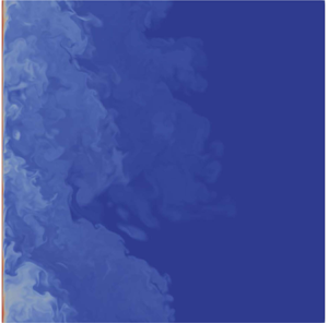
Figure 3 illustrates the flow field visualization of the turbulent NCBL flow for DNS-A at ${\textit {Gr}}_\delta = 7.7\times 10^7$. Due to the presence of the wall, a boundary layer has developed in the near-wall region whereas the outer bulk flow shows a plume-like structure. The fine structures in figure 3(a) and the magnified view of the temperature and velocity contours in the near-wall region, given in figure 3(b,c), indicate that the flow is turbulent with a large range of scales of motion. Similar turbulent structure is also observed in DNS-B, as shown in figure 2(h).

Figure 3. Visualization of the midspan flow field for DNS-A at ${\textit {Gr}}_\delta = 7.7\times 10^7$. (a) Temperature contours; (b) magnified temperature contours of the red box in panel (a); (c) magnified streamwise velocity contour of the red box in panel (a); dash-dotted line shows the maximum mean streamwise velocity location $\delta _m=34.25L_s$.

By the end of simulation, DNS-A has reached ${\textit {Gr}}_\delta =7.7\times 10^7$ ($\textit {Re}_\tau = 147.99$); while DNS-B has achieved ${\textit {Gr}}_\delta = 7.6\times 10^7$ ($\textit {Re}_\tau =120.32$). Here, the friction Reynolds number is given by

(3.1)\begin{equation} \textit{Re}_{\tau} = \frac{\delta_m {u_\tau} }{\nu}, \end{equation}

where ${u_\tau }$ is the friction velocity given by the wall shear stress $\tau _w$,

(3.2a,b)\begin{equation} {u_\tau} =\sqrt{{\tau_w}/\rho}, \quad \tau_w = \left. \rho\nu\frac{\partial \bar u}{\partial y}\right|_{y=0}. \end{equation}

The viscous length scale, $l_\tau$, is therefore given by

(3.3)\begin{equation} l_\tau = \frac{\nu}{u_\tau}. \end{equation}

The mean temperature and velocity profiles for the turbulent NCBL are fully described by the Reynolds averaged equations, where spatially averaging in homogeneous plane ($x\text {--}z$) is denoted by $\bar {(\cdot )}$. In wall units, the spatially averaged equations read

(3.4a)\begin{gather} \frac{l_\tau}{{{u_\tau}}^2}\frac{\partial (u^+ {u_{\tau}})}{\partial (t^+l_\tau/u_\tau)}= \frac{\partial ^2 u^+}{{\partial y^+}^2} -\frac{\partial (\overline{u'v'})^+}{\partial y^+}+{\textit{Ri}}_w-{\textit{Ri}}_\tau \theta^+, \end{gather}

(3.4b)\begin{gather}\frac{l_\tau}{ {{u_\tau}}{{\theta_\tau}}}\frac{\partial (\theta^+{{\theta_\tau}})}{\partial (t^+l_\tau/u_\tau)}= \frac{1}{Pr}\frac{\partial ^2 \theta^+}{\partial {y^+}^2}-\frac{\partial (\overline{v'\theta'})^+}{\partial y^+}, \end{gather}

where

(3.5a,b)\begin{equation} {\textit{Ri}}_{w} \equiv \frac{g \beta l_\tau\theta_w}{{{u_\tau}}^2}=\frac{g\beta \nu \theta_w}{u_\tau^3},\quad {\textit{Ri}}_{\tau} \equiv \frac{ g\beta l_\tau \theta_\tau }{{{u_\tau}}^2}=\frac{g\beta \nu q_w}{u_\tau^4}, \end{equation}

are the friction Richardson number based on wall temperature difference and friction temperature, respectively, $u^+$ and $\theta ^+$ are the mean temperature and velocity in wall units, defined as

(3.6a,b)\begin{equation} u^+ = \frac{\bar u}{{u_\tau}}, \quad \theta^+ = \frac{\theta_w-\bar \theta}{{{\theta_\tau}}}, \end{equation}

and $(\overline {u'v'})^+$ and $(\overline {v'\theta '})^+$ are the Reynolds shear stress and the turbulent heat flux in wall units, given by

(3.7a,b)\begin{equation} (\overline{u'v'})^+ = \frac{\overline{u'v'}}{{{u_\tau}}^2}, \quad (\overline{v'\theta '})^+ = -\frac{\overline{v'\theta '}}{{u_\tau} {{\theta_\tau}}}. \end{equation}

The friction temperature ${{\theta _\tau }}$ is given by the wall heat flux $q_w$ and the friction velocity ${u_\tau }$,

(3.8a,b)\begin{equation} {{\theta_\tau}} = \frac{q_w}{\rho C_p {u_\tau}}, \quad q_w =\left. -\rho C_p\kappa\frac{\partial \bar \theta}{\partial y}\right|_{y=0}, \end{equation}

where $C_p$ is the specific heat capacity of the fluid. Note the continuity equation (2.1a) vanishes as the derivatives in the homogeneous direction $\partial \bar {(\cdot )}/\partial x$ and $\partial \bar {(\cdot )}/\partial z$ and the mean wall-normal velocity $\bar v$ are all zero due to the parallel nature of the flow. From (3.4), a force balance and an energy balance can be obtained by integrating once with respect to the wall-normal distance $y^+$,

(3.9a)\begin{gather} \int_{0}^{y^+} \frac{l_\tau}{{{u_\tau}}^2}\frac{\partial (u^+ {u_{\tau}})}{\partial (t^+l_\tau/u_\tau)} \,\mathrm{d}y^+ =\left. \frac{\partial u^+}{\partial y^+}\right|^{y^+}_{0} - (\overline{u'v'})^+|^{y^+}_{0} + \int^{y^+}_{0}( {\textit{Ri}}_w-{\textit{Ri}}_\tau\theta^+ )\,\mathrm{d}y^+ , \end{gather}

(3.9b)\begin{gather}\int_{0}^{y^+} \frac{l_\tau}{ {{u_\tau}}{{\theta_\tau}}}\frac{\partial (\theta^+{{\theta_\tau}})}{\partial (t^+l_\tau/u_\tau)} \,\mathrm{d}y^+ = \left.\frac{1}{\textit{Pr}}\frac{\partial \theta^+}{\partial y^+}\right|^{y^+}_{0} - ( \overline{v' \theta '} )^+ |^{y^+}_{0}. \end{gather}

Given the boundary conditions at the wall, the integrated terms read

(3.10a)\begin{gather} \left.\frac{\partial u^+}{\partial y^+}\right|^{y^+}_{0} = \frac{\partial u^+}{\partial y^+} - 1, \end{gather}

(3.10b)\begin{gather}(\overline{u'v'})^+|^{y^+}_{0} =(\overline{u'v'})^+ , \end{gather}

(3.10c)\begin{gather}\left.\frac{1}{\textit{Pr}}\frac{\partial \theta^+}{\partial y^+}\right|^{y^+}_{0}=\frac{1}{\textit{Pr}}\frac{\partial \theta^+}{\partial y^+}-1, \end{gather}

(3.10d)\begin{gather}( \overline{v' \theta '} )^+ |^{y^+}_{0} = ( \overline{v' \theta '} )^+ , \end{gather}

the balance equations (3.9) are therefore reduced to

(3.11a)\begin{gather} \int_{0}^{y^+} \frac{l_\tau}{{{u_\tau}}^2}\frac{\partial (u^+ {u_{\tau}})}{\partial (t^+l_\tau/u_\tau)} \,\mathrm{d}y^+ = \frac{\partial u^+}{\partial y^+} - (\overline{u'v'})^+ + \int^{y^+}_{0}( {\textit{Ri}}_w-{\textit{Ri}}_\tau\theta^+)\,\mathrm{d}y^+ -1, \end{gather}

(3.11b)\begin{gather}\int_{0}^{y^+} \frac{l_\tau}{ {{u_\tau}}{{\theta_\tau}}}\frac{\partial (\theta^+{{\theta_\tau}})}{\partial (t^+l_\tau/u_\tau)} \,\mathrm{d}y^+ = \frac{1}{\textit{Pr}}\frac{\partial \theta^+}{\partial y^+} - ( \overline{v' \theta '} )^+ -1. \end{gather}

The individual contribution to the balance equations (3.11) are shown in figure 4. From figure 4(a), a constant heat flux region, where the molecular diffusion and turbulent heat flux balances the wall heat flux

(3.12)\begin{equation} q^+\equiv \frac{1}{\textit{Pr}}\frac{\partial \theta^+}{\partial y^+} - ( \overline{v' \theta '} )^+\sim 1, \end{equation}

is found for $y^+<150$ at ${\textit {Gr}}_\delta =7.7\times 10^7$. This is consistent with the existing literature (George & Capp Reference George and Capp1979; Hölling & Herwig Reference Hölling and Herwig2005; Wells & Worster Reference Wells and Worster2008) where a constant heat flux layer is identified in the near-wall region for the turbulent spatially developing NCBL. Our results in figure 4(b) also show that an equilibrium is reached by the wall shear and the driving forces (buoyancy force and shear stress), where

(3.13)\begin{equation} F^+\equiv \frac{\partial u^+}{\partial y^+} - (\overline{u'v'})^+ + \int^{y^+}_{0}( {\textit{Ri}}_w-{\textit{Ri}}_\tau\theta^+ )\,\mathrm{d}y^+ \sim 1, \end{equation}

so that a constant forcing region ($F^+$ independent of $y^+$) is obtained. In the present study, we define the limit of the constant forcing region as the point where $F^+$ exceeds the wall shear stress $\tau _w^+$ by $10\,\%$, i.e. $F^+=1.1$. For ${\textit{Gr}} _\delta =7.7\times 10^7$ (DNS-A), this gives a constant forcing region up to $y^+=150$ (which is approximately $y=\delta _m$). At lower ${\textit {Gr}}_\delta$, as indicated by figure 4(c), this constant forcing region extends to $y^+= 60$($y=0.6\delta _m$) for ${\textit {Gr}}_\delta = 2.1\times 10^7$ (DNS-A); $y^+=70$ ($y=0.6\delta _m$) for ${\textit {Gr}}_\delta =4.1\times 10^7$ (DNS-A); and $y^+=100$ ($y=0.8\delta _m$) for ${\textit {Gr}}_\delta =7.6\times 10^7$ (DNS-B).

Figure 4. The near-wall statistics: (a) heat flux balance at ${\textit {Gr}}_\delta =7.7\times 10^7$ (DNS-A); (b) force balance at ${\textit {Gr}}_\delta =7.7\times 10^7$ (DNS-A); (c) force balances at ${\textit {Gr}}_\delta =2.1\times 10^7$ (DNS-A), ${\textit {Gr}}_\delta =4.1\times 10^7$ (DNS-A) and ${\textit {Gr}}_\delta =7.6\times 10^7$ (DNS-B), with molecular shear $\partial u^+/\partial y^+$ (dash-dotted lines), Reynolds shear stress $-\overline {u'v'}$ (dashed lines), buoyancy force $\int _0^{y^+} ( {\textit {Ri}}_w-{\textit {Ri}}_\tau \theta ^+ )\,\mathrm {d}y^+$ (dotted lines) and total force $F^+$ (solid lines); vertical dashed lines indicate the location when $F^+=1.1$ at corresponding ${\textit {Gr}}_\delta$.

In the constant flux (and constant forcing) region, the right-hand sides of (3.11a) and (3.11b) both sum to zero, indicating the temporal evolution of the momentum and temperature (left-hand sides) are indeed negligible, and thus there exists a slowly varying near-wall region. With this in mind, the temporal evolution of the flow in the near-wall region can be ignored and for the purposes of developing mean profiles, a steady flow is assumed at each time instant.

4. Wall characteristics

Figure 5 depicts the development of the heat transfer of the NCBL in terms of Nusselt number ${\textit {Nu}}_\delta$ and the wall shear stress (normalized by the boundary layer thickness $\delta$) with ${\textit {Gr}}_\delta$ (which grows with time $t$ only). Here, the Nusselt number and the normalized wall shear are given by

(4.1a,b)\begin{equation} {\textit{Nu}}_{\delta} \equiv \frac{\delta q_w}{\rho C_p\kappa\theta_w},\quad \tau_w^*= \tau_w/\rho g\beta\theta_w\delta. \end{equation}

Figure 5. Temporal development of the wall characteristics: (a) Nusselt number; (b) wall shear stress; (c) the friction Reynolds number. The grey diamond symbols represent the data points shown in figure 2 for DNS-B.

At low ${\textit {Gr}}_\delta$, the Nusselt number and the normalized wall shear stress are ${\textit {Gr}}_\delta$ independent, giving

(4.2a,b)\begin{equation} {\textit{Nu}}_\delta = \frac{1.71}{\sqrt{\rm \pi}}=0.965, \quad \tau_w^* = 0.302, \end{equation}

according to the analytical solution (2.3) in the laminar conductive regime (e.g. Ke et al. Reference Ke, Williamson, Armfield, McBain and Norris2019). At approximately ${\textit {Gr}}_\delta =10^6$, the spatially developing flows (Cheesewright Reference Cheesewright1968; Tsuji & Nagano Reference Tsuji and Nagano1988; Nakao et al. Reference Nakao, Hattori and Suto2017) undergo transition to turbulence. In this regime, the wall shear stress and the Nusselt number are found to follow the empirical formula,

(4.3a,b)\begin{equation} {\textit{Nu}}_\delta = 0.107{\textit{Gr}}_\delta^{1/3}, \quad \tau_w^*= 1.01{\textit{Gr}}_\delta^{-8/35.7}\approx1.01{\textit{Gr}}_\delta^{-2/9}. \end{equation}

However, the temporally developing NCBL at ${\textit {Gr}}_\delta \sim 10^6$ is not yet turbulent for the present study. For case DNS-B, two ‘reversed’ Grashof number regions, in which the ${\textit {Gr}}_\delta$ gradually reduces, can be observed at ${\textit {Gr}}_\delta \sim 10^6$ and ${\textit {Gr}}_\delta \sim 7\times 10^6$. These unusual reverses in ${\textit {Gr}}$ are found to be closely related to the pathway of the laminar–turbulent transition (the aforementioned detachment of the convective rolls in figure 2) as ${\textit {Gr}}_\delta$ is given by the shape of the velocity profile in the laminar–turbulent transition process (Ke et al. Reference Ke, Williamson, Armfield, Norris and Kirkpatrick2018). Nevertheless, at ${\textit {Gr}}_\delta > 10^7$ the Nusselt number for the temporal cases start to share a similar exponential correlation as the empirical formula for the spatially developing NCBL with a different constant, such that

(4.4)\begin{equation} {\textit{Nu}}_\delta=K_q{\textit{Gr}}_\delta^{1/3},\end{equation}

where $K_q=0.098$ for case DNS-A, while DNS-B has $K_q=0.085$ for $1.0\times 10^7<{\textit {Gr}}_\delta <5.0\times 10^7$ but appears to converge to $K_q=0.098$ over $5.0\times 10^7<{\textit {Gr}}_\delta <7.6\times 10^7$. In a more recent study, Ng et al. (Reference Ng, Ooi, Lohse and Chung2017) obtained the empirical scaling

(4.5)\begin{equation} {\textit{Nu}}_\delta\sim {\textit{Gr}}_\delta^{0.37},\end{equation}

by conditionally averaging on high wall shear events in their DNS of natural convection in a vertical differentially heated slot. The authors show that their empirical scaling relation given in (4.5) is consistent with the $1/2$-power-law scaling with a logarithmic correction in homogeneous Rayleigh–Bènard convection, where the boundary layer is dominated by the bulk thermal convection (ultimate regime when ${\textit {Gr}}_\delta$ is asymptotically high) in the sense of Grossmann & Lohse (Reference Grossmann and Lohse2000, Reference Grossmann and Lohse2011). The difference between (4.4) and (4.5) is somewhat subtle in the current ${\textit {Gr}}_\delta$ range of ${\textit {Nu}}_\delta$ results shown in figure 5 (up to ${\textit {Gr}}_\delta \sim 7.7\times 10^7$ for DNS-A and ${\textit {Gr}}_\delta \sim 7.6\times 10^7$ for DNS-B). The temporal nature of our DNS means turbulence shows up in the instantaneous ${\textit {Nu}}_\delta$ which makes detecting small changes in the ${\textit {Nu}}_\delta$–${\textit {Gr}}_\delta$ scaling without a large ${\textit {Gr}}_\delta$ range difficult. Using empirical relationships for forced boundary layers, Wells & Worster (Reference Wells and Worster2008) showed that at very high ${\textit {Gr}}_{\delta }$ the spatially developing vertical NCBL may attain a ${\textit {Nu}}_\delta \sim {\textit {Gr}}_{\delta }^{1/2}$ scaling which for the present flow is estimated above ${\textit {Gr}}_{\delta } \sim O(10^{10})$. In the current ${\textit {Gr}}_\delta$ range, we do not yet see evidence for ${\textit {Nu}}_\delta \sim {\textit {Gr}}_{\delta }^{1/2}$ in our ${\textit {Nu}}_\delta$ results shown in figure 5(a).

Similar behaviour can also be found in the wall shear stress: the temporal cases start to follow the empirical exponential correlation with larger constants at ${\textit {Gr}}_\delta >10^7$,

(4.6)\begin{equation} \tau_w^* =K_\tau {\textit{Gr}}_\delta^{-8/35.7}\approx K_\tau {\textit{Gr}}_\delta^{-2/9},\end{equation}

where $K_\tau =1.52$ for case DNS-A and $K_\tau = 1.33$ for case DNS-B. Notably, the temporal DNS of Abedin et al. (Reference Abedin, Tsuji and Hattori2009) also indicates a larger constant for wall shear than the empirical correlation. Since the wall characteristics of the temporally developing NCBL exhibit similar scaling relations to the turbulent spatially developing NCBL at ${\textit {Gr}}_\delta >10^7$, we therefore refer to this regime as the turbulent regime for the temporally developing NCBL. The collapse of the wall characteristics in the turbulent regime indicate the NCBL obtained in DNS-A and DNS-B are, in some sense, initial condition-invariant: although the flow in DNS-B undergoes a weakly three-dimensional transition due to the difference in the initial condition, it still shares common features that can also observed in DNS-A in the turbulent regime – with a different constant. This can also be seen in figure 5(c) where the $\textit {Re}_\tau$ for DNS-B is approaching the $\textit {Re}_\tau$ in DNS-A as the ${\textit {Gr}}_\delta$ increases. For clarity we present the results of DNS-A in the following sections unless otherwise specified. A detailed comparison of DNS-A and DNS-B will be given in § 6.4.

5. Profiles in the laminar-like sublayer

The mean temperature gradient in the slowly time-varying region can be obtained by integrating (3.4b) such that

(5.1)\begin{equation} \mathcal{C}\sim \frac{1}{\textit{Pr}}\frac{\partial \theta^+}{\partial {y^+}}-(\overline{v'\theta'})^+,\end{equation}

where $\mathcal {C}$ is a constant resulting from performing the integration. In the close vicinity of the wall, (5.1) can be further simplified provided the turbulent transport $(\overline {v'\theta '})^+$ in this region is negligible, so that

(5.2)\begin{equation} \theta^+\sim \mathcal{C}\textit{Pr} y^+ + \mathcal{D},\end{equation}

is obtained after integrating (5.1) along the wall-normal direction. Here, $\mathcal {D}$ is also a constant resulting from performing the integration. Employing the boundary condition at ${y^+=0}, \theta ^+=0$ and $(1/\textit {Pr}) (\partial \theta ^+/\partial y^+)= q_w^+$, the near-wall temperature profile is obtained as

(5.3)\begin{equation} \theta^+=\textit{Pr} y^+.\end{equation}

This suggests that the mean temperature follows a linear relation in the close vicinity of the wall for the temporally developing NCBL, as reported by several NCBL studies (Tsuji & Nagano Reference Tsuji and Nagano1988; Hölling & Herwig Reference Hölling and Herwig2005; Ng et al. Reference Ng, Ooi, Lohse and Chung2017). Similarly, by assuming a slowly varying flow and neglecting the Reynolds shear stress in this region, the mean velocity profile is dominated by the buoyancy force in the region and can be obtained by integrating (3.4a) twice in the wall-normal direction, giving

(5.4)\begin{equation} u^+\sim\iint -({\textit{Ri}}_w-{\textit{Ri}}_\tau \theta^+) \,\mathrm{d}y^+\,\mathrm{d}y^+.\end{equation}

The temperature coupling term, $\theta ^+$, in (5.4) is then replaced by the linear relation (5.3). After applying the boundary conditions at the wall ($y^+=0$), i.e. $u^+=0$ and $\partial u^+/\partial y^+ = \tau _w^+$, gives

(5.5)\begin{equation} u^+= y^+ - \frac{1}{2}{\textit{Ri}}_{w}{y^+}^2+\frac{\textit{Pr}}{6}{\textit{Ri}}_{\tau}{y^+}^3,\end{equation}

in the near-wall region. Unlike the mean temperature profile, the mean velocity profile for the NCBL does not feature a linear region, as is commonly found in the viscous sublayer for the momentum-dominated flows. This is due to the presence of the extra buoyancy terms. The coefficients ${\textit {Ri}}_{w}$ and ${\textit {Ri}}_{\tau }$ clearly indicate the ${\textit {Gr}}_\delta$-dependency of the mean streamwise velocity profile. Such modification of the mean profile takes a similar form to the pressure gradient effect described by Nickels (Reference Nickels2004) for wall bounded flows subjected to large pressure gradients. The existence of two Richardson numbers is a result of the two temperature scales in the problem: ${\textit {Ri}}_w$ represents the bulk temperature difference $\theta _w = T_w-T_\infty$ which provides the driving force for buoyancy and ${\textit {Ri}}_\tau$ indicates a wall heat flux quantity $\theta _\tau$ which scales the near-wall temperature gradients. A similar analysis can also be seen in Hölling & Herwig (Reference Hölling and Herwig2005), where they have used the temperature gradients to identify the characteristic velocity, so that the buoyancy dependency is absorbed into the normalized coordinates. The near-wall mean profiles obtained here, given in (5.3) and (5.5), are consistent with the result Tsuji & Nagano (Reference Tsuji and Nagano1988) obtained using a Taylor series expansion and the solution by Wells & Worster (Reference Wells and Worster2008) for spatially developing NCBLs.

Figure 6 shows the near-wall mean temperature and velocity profiles in wall units from the DNS data. The mean temperature $\theta ^+$, according to figure 6(a), shows a linear relationship in the near-wall region, as described by (5.3) for $y^+<5$. However, according to figure 6(b), the viscous sublayer that is commonly found in the momentum-dominated flows in which region the linear relation

(5.6)\begin{equation} u^+=y^+,\end{equation}

holds does not exist in the NCBL, as predicted by (5.5). A similar observation is also made by Tsuji & Nagano (Reference Tsuji and Nagano1988) for a spatially developing NCBL, and Ng et al. (Reference Ng, Ooi, Lohse and Chung2017) for a differentially heated NCBL channel flow. From (5.5), the absence of the linear velocity profile (5.6) for the NCBL in the near-wall region is essentially due to the extra buoyancy, which can be seen in figure 7 where the buoyancy contribution to the mean velocity profile is shown in wall units. From figure 7, it is clear that the buoyancy contribution is negative and gradually approaches to zero as the flow reaches higher ${\textit {Gr}}_\delta$. The physical interpretation is rather simple: as the flow progressively achieves higher ${\textit {Gr}}_\delta$ in the turbulent regime, the friction velocity ${u_\tau }$ is gradually growing in magnitude due to the increase in the wall shear stress ${\tau _w}$. According to (4.4) and (4.6), the friction velocity ${u_\tau }$ and the wall heat flux $q_w$ in the turbulent regime follow the scaling relation

(5.7a)\begin{gather} {u_\tau} = K_\tau^{1/2}(g\beta\theta_w\nu)^{1/3}{\textit{Gr}}_\delta^{1/18}, \end{gather}

(5.7b)\begin{gather}q_w = K_q (g\beta)^{1/3}\theta_w^{4/3}\rho C_p\kappa \nu^{-2/3}. \end{gather}

Figure 6. (a) Mean temperature profiles for the turbulent NCBL at different ${\textit {Gr}}_\delta$; (b) mean velocity profiles for the turbulent NCBL at different ${\textit {Gr}}_\delta$; the markers represents the experimental measurements of Tsuji & Nagano (Reference Tsuji and Nagano1988) for a spatially developing NCBL with $\textit {Pr} =0.71$.

Figure 7. Buoyancy contribution to the mean velocity profile in wall units.

It can be seen the wall heat flux $q_w$ in the turbulent regime is a constant (independent of ${\textit {Gr}}_\delta$), suggesting the friction Richardson numbers depend solely on the friction velocity (or, the wall shear), such that

(5.8a,b)\begin{equation} {\textit{Ri}}_w \sim \frac{1}{u_\tau^3} \sim {\textit{Gr}}_\delta^{-1/6}, \quad {\textit{Ri}}_{\tau} \sim \frac{1}{u_\tau^4} \sim {\textit{Gr}}_\delta^{-2/9}. \end{equation}

The buoyancy contribution thus asymptotically approaches zero,

(5.9)\begin{equation} -\frac{1}{2}{\textit{Ri}}_{w}{y^+}^2+\frac{\textit{Pr}}{6}{\textit{Ri}}_{\tau}{y^+}^3 \sim 0 ,\end{equation}

at some large ${u_\tau }$ (or, identically, large ${\textit {Gr}}_\delta$). Figure 8 depicts the development of the friction Richardson numbers. It can be seen that both ${\textit {Ri}}_{w}$ and ${\textit {Ri}}_{\tau }$ qualitatively agree with the empirical correlation (5.8a,b) in the turbulent regime.

Figure 8. Development of the friction Richardson numbers with ${\textit {Gr}}_\delta$: (a) ${\textit {Ri}}_w$; (b) ${\textit {Ri}}_\tau$.

Further justification can be obtained by restarting the NCBL DNS-A in the turbulent regime, but having the temperature field uncoupled from the velocity field. The uncoupling of the temperature field is achieved by removing the buoyancy forcing term $\theta \delta _{i1}$ from the governing equation (2.1b) so that the temperature now acts as a passive scalar and the flow is completely dominated by the momentum. One may consider the uncoupled flow as a planar jet flow adjacent to the wall with an initial velocity profile taken from that of a turbulent NCBL. Figure 9 shows the comparison of the near-wall mean velocity profiles of the two flows. The near-wall mean velocity profile of the turbulent NCBL, according to figure 9, has an excellent agreement with (5.5) for $y^+<5$, beyond which point the turbulent transport becomes non-negligible; whereas the uncoupled case quickly recovers and matches the linear relation (5.6) for $y^+<5$ since the buoyancy effect is absent. This can be seen from the inset of figure 9, where the ratio $u^+/y^+$ at $y^+=5$ increases from $93.5\,\%$ (which is given by the NCBL profile as initial condition) to $98.6\,\%$ at $t^+=7.1$ and remains around $99\,\%$ subsequently.

Figure 9. Comparison of the near-wall mean velocity profile of the NCBL and the temperature field uncoupled flow; the uncoupled flow uses the NCBL at ${\textit {Gr}}_\delta = 4.72\times 10^7$ as an initial condition ($t^+=0$). Inset shows the temporal development of $u^+/y^+$ at $y^+\sim 5$ for the uncoupled flow.

6. The logarithmic region

Further away from the wall, a logarithmic region, where

(6.1)\begin{equation} \theta^+ = \frac{\textit{Pr}_t}{K_v} \ln(y^+)+B_\theta,\end{equation}

can be found for the mean temperature profile for $y^+>50$ in figure 10(a). Here, $\textit {Pr}_t$ is the turbulent Prandtl number, $K_v$ is the von Kármán constant and $B_\theta$ is a universal constant. Similar observations of the near-wall temperature structures are also made by the experimental measurements of a spatially developing turbulent NCBL (Tsuji & Nagano Reference Tsuji and Nagano1988), where they identified the logarithmic region to be $30<y^+<200$ for Grashof number up to ${\textit {Gr}}_\delta = 1\times 10^7$ and the constant to be $\textit {Pr}_t/K_v =1.45$. However, we have adopted the same constants as Yaglom (Reference Yaglom1979) and Ng et al. (Reference Ng, Ooi, Lohse and Chung2017) for better agreement with our numerically generated data, i.e. $\textit {Pr}_t = 0.85$ and $K_v = 0.41$. According to the spatially developing experiment by Tsuji & Nagano (Reference Tsuji and Nagano1988), the constant $B_\theta$ appears to depend on, and vary with ${\textit {Gr}}_\delta$; whereas from figure 10(a), it can be seen that the temperature profiles agree well with (6.1) in the logarithmic region with the constant $B_\theta =7.5$, regardless of the value of ${\textit {Gr}}_\delta$. However, it should be noted that the data from Tsuji & Nagano (Reference Tsuji and Nagano1988) are at relatively low ${\textit {Gr}}_\delta$ when compared with the current study.

Figure 10. (a) Mean temperature profiles for the turbulent NCBL at different ${\textit {Gr}}_\delta$. (b) Mean velocity profiles for the turbulent NCBL at different ${\textit {Gr}}_\delta$; with $K_v=0.41, Pr_t=0.85, B_\theta =7.5$ and $B_u=5$. The markers represents the experimental measurements of Tsuji & Nagano (Reference Tsuji and Nagano1988) for a spatially developing NCBL with $\textit {Pr} =0.71$.

The mean velocity profiles, however, as shown in figure 10(b), demonstrate a strong ${\textit {Gr}}_\delta$ dependency. From figure 10(b), the conventional log-law region, given by

(6.2)\begin{equation} u^+=\frac{1}{K_v}\ln(y^+)+B_u,\end{equation}

cannot be observed for the NCBL even at ${\textit {Gr}}_\delta =7.7\times 10^7$. Here, $B_u=5$ is a constant for the results presented. The difference between the velocity profiles and the conventional log-law (6.2) becomes more significant with increasing ${\textit {Gr}}_\delta$ as the velocity profiles grow in magnitude and do not exhibit a log-law region in the classical sense. Note the maximum velocity $u_{m}^+$ is also increasing with ${\textit {Gr}}_\delta$ (or $\textit {Re}_\tau$) since the characteristic velocity $u_\tau$ does not contain any buoyancy information. A direct consequence is that the difference here (between the velocity profiles and the conventional log-law) is somewhat different from the overshoot of the conventional log-law in the sense of Nickels (Reference Nickels2004) and Chan et al. (Reference Chan, MacDonald, Chung, Hutchins and Ooi2015) due to low $\textit {Re}_\tau$ effects. The above observation is consistent with previously reported behaviour (Tsuji & Nagano Reference Tsuji and Nagano1988; Ng et al. Reference Ng, Ooi, Lohse and Chung2017). The absence of the conventional log-law for the velocity profile is not surprising as (6.2) does not take the buoyancy effect into account. We hereby propose a modified velocity profile prediction for the NCBL in the conventionally thought log-law region (where the flow varies slowly in time in the sense of figure 4 and the temperature has a log-law profile, $50<y^+<150$ for our results at ${\textit {Gr}}_\delta = 7.7\times 10^7$) by taking the buoyancy effect into consideration. The mean velocity profile in this region is obtained by integrating the velocity gradient, which can be solved from (3.11a) given the temporal derivative is zero. However, the Reynolds stress and the buoyancy force in (3.11a) are not yet analytically known and thus require appropriate modelling.

6.1. Buoyancy force approximation

The buoyancy force $F_b^+$ is fully described by the temperature profile $\theta ^+$ as follows:

(6.3)\begin{equation} F_b^+ \equiv \int^{y^+}_{0} ( {\textit{Ri}}_w - {\textit{Ri}}_\tau\theta^+ )\,\mathrm{d}y^+ = {\textit{Ri}}_w y^+- {\textit{Ri}}_\tau \int^{y^+}_{0} \theta^+\,\mathrm{d}y^+, \end{equation}

since ${\textit {Ri}}_w$ and ${\textit {Ri}}_\tau$ are both constants at a given ${\textit {Gr}}_\delta$. In the present study, the buoyancy force given in (6.3) is approximated by two approaches to simplify the analysis.

6.1.1. Log-law approximation

From figure 10(a), the temperature profile follows the log-law relation (6.1). Upon integration of (6.3) with respect to $y^+$ after the substitution of (6.1), the buoyancy force in the temperature log-law region can therefore be approximated by

(6.4)\begin{equation} F_ b^+ = C_1 y^+ + {\textit{Ri}}_\tau K_1-{\textit{Ri}}_\tau\frac{\textit{Pr}_t}{K_v}\ln{({y^+})}y^+, \end{equation}

where the proportionality coefficient $C_1$ is given by

(6.5)\begin{equation} C_1 = {\textit{Ri}}_w-{\textit{Ri}}_\tau\left(B_\theta-\frac{\textit{Pr}_t}{K_v}\right) \end{equation}

and $K_1$ is an unknown constant from integration. A similar approximation for the buoyancy force has also been applied by Wei (Reference Wei2019) to approximate the Reynolds shear stress in the differentially heated vertical channel NCBL flows. Empirically, by fitting (6.4) with the DNS data at $y^+=50$ (see figure 11), we have found

(6.6)\begin{equation} K_1 = 150, \end{equation}

is a constant for the ${\textit {Gr}}_\delta$ range presented in the turbulent regime. As shown in figure 11, the integral constant $K_1$ sets the magnitude (vertical shift) of the buoyancy force when multiplied by ${\textit {Ri}}_\tau$ in (6.4) at different ${\textit {Gr}}_\delta$. Our results suggest that $K_1$ does not have ${\textit {Gr}}_\delta$ dependency since the temperature profiles in DNS-A are self-similar: we will show later in § 6.4 that for the non-self-similar temperature profiles in DNS-B and the spatially developing measurements of Tsuji & Nagano (Reference Tsuji and Nagano1988) $K_1$ gradually approach to the constant obtained here by DNS-A as the flow achieves higher ${\textit {Gr}}_\delta$.

Figure 11. Comparison of the approximations of the buoyancy force at ${\textit {Gr}}_\delta =2.1\times 10^7, {\textit {Gr}}_\delta =4.1\times 10^7$ and ${\textit {Gr}}_\delta =7.7\times 10^7$; lines show the DNS data; circle markers show the approximations by (6.4) with $K_1=150$; square markers show the approximations by (6.7).

6.1.2. Linear approximation

The approximation of the buoyancy force (6.3) can be further simplified due to the fact that the $\theta ^+$ is changing only slightly in the temperature log-law region ($y^+>50$). By treating $\theta ^+$ as a constant in the temperature log-law region, (6.3) becomes

(6.7)\begin{equation} F_b^+ = {C_2}y^++A_2 , \end{equation}

where ${C_2}$ is a proportionality coefficient given by

(6.8)\begin{equation} C_2={\textit{Ri}}_w-{\textit{Ri}}_\tau\varTheta^+ \end{equation}

and the intercept $A_2$ is given by

(6.9)\begin{equation} A_2=K_2{\textit{Ri}}_\tau, \end{equation}

where $K_2$ is an unknown constant representing the difference between the linear approximation (6.7) and the nonlinear growth of the buoyancy force before the log-law region. Empirically, by matching the DNS data with (6.7) at $y^+=50$ we have found

(6.10)\begin{equation} K_2 = 280, \end{equation}

for the data shown. Here, $\varTheta ^+$ is the mean value of $\theta ^+$ in the region. In the present study, $\varTheta ^+=16$ is used (see the temperature profiles in figure 10). Similar to $K_1$, the constants $K_2, B_\theta$ and $\varTheta ^+$ obtained here appear universal in our ${\textit {Gr}}_\delta$ range due to the self-similar temperature profiles in DNS-A. Evidently, when multiplied by ${\textit {Ri}}_\tau$, the constant $K_2$ also accounts for the ${\textit {Gr}}_\delta$ dependency (see figure 11). The buoyancy force modelled by the linear relation (6.7) therefore depends solely on the wall characteristics since the proportionality coefficient ${C_2}$ and the intercept $A_2$ varies with ${{\textit {Ri}}_w}$ and ${{{\textit {Ri}}_\tau }}$ only.

Figure 11 shows the comparison of the approximation of the buoyancy force given by (6.4) and (6.7) with the DNS data at different ${\textit {Gr}}_\delta$. According to figure 11, the buoyancy force $F_b^+$ decreases with increasing ${\textit {Gr}}_\delta$ due to the increasing friction velocity ${u_\tau }$. Both (6.4) and (6.7) show good agreement with the DNS data in the temperature log-law region $y^+>50$. The agreement between the approximations and the actual DNS data improves with increasing ${\textit {Gr}}_\delta$.

6.2. Reynolds stress approximation

In conventional momentum-dominated wall-bounded flows, the local momentum transfer by the Reynolds shear stress is frequently modelled by the Prandtl mixing length model (Prandtl Reference Prandtl1925),

(6.11)\begin{equation} - (\overline{u'v'})^+ = {l_m^+}^2 \left(\frac{\partial u^+}{\partial y^+}\right)^2,\end{equation}

where $l_m^+$ is the mixing length. The presence of the wall, according to Townsend (Reference Townsend1976), imposes a turbulent length scale on the velocity field so that the main eddies of the flow are, in a sense, ‘attached’ to the wall. In other words, the turbulent length scale of the large eddies (Townsend Reference Townsend1961),

(6.12)\begin{equation} L\equiv \frac{k^{3/2}}{\varepsilon}, \end{equation}

is expected to scale with the wall-normal distance $y^+$. Here, $k$ and $\varepsilon$ are the turbulent kinetic energy and the turbulent kinetic energy dissipation rate, respectively, defined by

(6.13a,b)\begin{equation} k=\frac{1}{2}\overline{{{u_i}'}^2}, \quad \varepsilon = \nu \overline{{\left(\frac{\partial {u_i}'}{\partial x_j}\right)}^2}. \end{equation}

Consequently, the mixing length is also expected to vary linearly with $y^+$ owing to the fact that the mixing length $l_m^+$ is proportional to $L$ in the log-law region for $y^+>50$ (see, for example, Townsend Reference Townsend1961; Pope Reference Pope2000, pp. 288–290), such that

(6.14)\begin{equation} L^+ = \frac{L}{l_\tau} \propto l_m^+ \propto y^+, \end{equation}

and the mixing length can be described by

(6.15)\begin{equation} l_m^+ = Dy^+, \end{equation}

where the proportionality coefficient $D$ is known as the von Kármán constant $K_v$ in the conventional momentum-dominated flows.

Since the NCBL is also bounded by the wall, it is convenient to assume the Reynolds shear stress shares a similar behaviour to the momentum-dominated flows and can be modelled by (6.11) and (6.15). The validity of applying (6.15) to the NCBL may be justified by examining the turbulent length scale $L$. As depicted in figure 12, the turbulent length scale $L$ follows a linear relation with $y^+$ at sufficiently high ${\textit {Gr}}_\delta$ (or, $\textit {Re}_\tau$) in the turbulent regime in the range $10<y^+<100$, indicating a mixing length $l^+_m$ proportional to $y^+$ as given in (6.15). However, it should be noted that the coefficient $D$ in (6.15) for NCBL remains unknown and may have a ${\textit {Gr}}_\delta$ dependency. In the present study, the coefficient $D$ is obtained empirically by rearranging (6.11),

(6.16)\begin{equation} D= \left[ \frac{- (\overline{u'v'})^+ }{({\partial u^+}/{\partial y^+})^{2} {y^+}^2}\right]^{1/2}. \end{equation}

According to figure 13, it can be seen that the ratio $-(\overline {u'v'})^+/(\partial u^+/\partial y^+)^2$ scales well with ${y^+}^2$ in the temperature log-law region for $y^+>50$ (see inset), and the coefficient $D$, with this more sensitive measure (6.16), shows minimal ${\textit {Gr}}_\delta$-dependency in our ${\textit {Gr}}_\delta$ range. Here, we choose

(6.17)\begin{equation} D= 0.3, \end{equation}

for the following analysis. It should be noted that the negative values of $-(\overline {u'v'})^+$ are prohibited by the nature of the mixing length model (6.11), we therefore shall only focus on the region where $-(\overline {u'v'})^+$ is positive (up to $y^+\sim 90$ for ${\textit {Gr}}_\delta =7.7\times 10^7$) in the present study.

Figure 12. The turbulent length scale in wall unit $L^+$ against the wall-normal distance $y^+$ for DNS-A at ${\textit {Gr}}_\delta =2.1\times 10^7, {\textit {Gr}}_\delta =4.1\times 10^7$ and ${\textit {Gr}}_\delta =7.7\times 10^7$; and for DNS-B at ${\textit {Gr}}_\delta =7.6\times 10^7$.

Figure 13. Proportionality coefficient $D$ at different ${\textit {Gr}}_\delta$: black dotted, ${\textit {Gr}}_\delta =2.1\times 10^7$; blue dashed, ${\textit {Gr}}_\delta =4.1\times 10^7$; red solid, ${\textit {Gr}}_\delta =7.7\times 10^7$. Inset shows the ratio $D^2 {{y^+}^2}=-(\overline {u'v'})^+/(\partial u^+/\partial y^+)^2$.

6.3. Modified log-law

Making use of (6.11), the force balance equation (3.11a) can be rewritten as a quadratic equation about the velocity gradient $\partial u^+/\partial y^+$,

(6.18)\begin{equation} \frac{\partial u^+}{\partial y^+}+{l_m^+}^2\left( \frac{\partial u^+}{\partial y^+}\right)^2 + F_b^+ = \tau_w^+. \end{equation}

The mean velocity gradient $\partial u^+/\partial y^+$ is therefore obtained as the solution to the quadratic equation (6.18). Note for NCBL, the velocity grows in the log-law region until it reaches its maximum and therefore a positive velocity gradient is expected,

(6.19)\begin{equation} \frac{\partial u^+}{\partial y^+} = \frac{-1+ [ 1+4{l_m^+}^2(\tau_w^+-F_b^+)]^{1/2}}{2{l_m^+}^2}.\end{equation}

When the buoyancy force $F_b^+$ is absent (for momentum-dominated flows or when buoyancy force is negligible, i.e. ${\textit {Gr}}_\delta \sim \infty$), (6.19) reduces to the ordinary velocity gradient equation for the conventional velocity log-law region in the momentum-dominated flows (see, for example, Buschmann & Gad-el Hak Reference Buschmann and Gad-el Hak2005). A similar method was also adapted by Granville (Reference Granville1989) and Buschmann & Gad-el Hak (Reference Buschmann and Gad-el Hak2005) when deriving the velocity log-law region for the wall-bounded turbulent boundary layers. In their analysis a constant shear layer, where $\partial u^+/\partial y^+ - (\overline {u'v'}^+)=\tau _w^+$, is assumed, whereas in the present study the total force in the near-wall region is a constant as shown in figure 4(b).

Owing to the fact that the molecular shear stress is negligible in this region (see also, figure 4), (6.18) reduces to a more convenient form,

(6.20)\begin{equation} {l^+_m}^2\left(\frac{\partial u^+}{\partial y^+}\right)^2 = {\tau_w^+-F_b^+}.\end{equation}

With $\tau _w^+=1$, the buoyancy force $F_b^+$ in (6.20) is then replaced by the approximations given in § 6.1. By applying the logarithmic approximation (6.4), the velocity gradient is obtained as

(6.21)\begin{equation} \widehat{\frac{\partial u^+}{\partial y^+}} = \frac{\sqrt{1-C_1y^+ - {\textit{Ri}}_\tau K_1 +{\textit{Ri}}_\tau\dfrac{\textit{Pr}_t}{K_v}\ln{(y^+)}y^+ }}{Dy^+}. \end{equation}

Alternatively, by applying the linear approximation of the buoyancy force given in (6.7), (6.20) can be reduced to

(6.22)\begin{equation} \widetilde{ \frac{\partial u^+}{\partial y^+}} = \frac{\sqrt{1-{C_2}y^+-A_2}}{Dy^+}. \end{equation}

Note when ${\textit {Gr}}_\delta$ asymptotically goes to infinity, both ${C_2}$ and $A_2$ go to zero due to large ${u_\tau }$ and (6.22) takes the form of the conventional momentum-dominated log-law region, i.e. $\partial u^+/\partial y^+= 1/(D y^+)$. Figure 14 compares the actual velocity gradient obtained by the DNS data with the predictions by (6.21) and (6.22). Both predictions show excellent agreement with the DNS data in the range $50<y^+<90$ since the buoyancy force and the Reynolds shear stress are correctly approximated and modelled. The mean velocity profile is therefore obtained as

(6.23)\begin{equation} u^+ = \int_0^{y_{c}^+} \frac{\partial u^+}{\partial y^+}\,\mathrm{d}y^++\int_{y_{c}^+}^{y^+} \frac{\partial u^+}{\partial y^+}\,\mathrm{d}y^+, \end{equation}

where $y_c^+$ is the starting point of the log-law region for the velocity profile. In the present study, it is assumed that the velocity log-law region starts at the same location as the temperature log-law region, i.e. $y^+_c=50$. Evidently, the first integration in (6.23) yields

(6.24)\begin{equation} \int_0^{y_{c}^+} \frac{\partial u^+}{\partial y^+}\,\mathrm{d}y^+ = u^+_c, \end{equation}

where $u^+_c$ is a constant given by the velocity magnitude at location $y^+={y^+_c}$. Recall that there is a buoyancy contribution in $y^+<50$, so the magnitude of $u^+_c$ is expected to depend on the wall characteristics, i.e. ${u_\tau }$ and ${{\theta _\tau }}$, and thus on ${\textit {Gr}}_\delta$, as demonstrated by figure 15.

Figure 14. The mean velocity gradient obtained from DNS-A at ${\textit {Gr}}_\delta =7.7\times 10^7$ and the predictions made by (6.21) and (6.22); with experimental measurements from Tsuji & Nagano (Reference Tsuji and Nagano1988) for a spatially developing NCBL at lower ${\textit {Gr}}_\delta$. Inset shows an enlarged view near the modified log-law region.

Figure 15. The development of the velocity magnitude $u^+_c$ ($u^+$ at $y^+=50$) against ${\textit {Gr}}_\delta$; the red circles mark the $u^+_c$ value used for ${\textit {Gr}}_\delta =2.1\times 10^7, {\textit {Gr}}_\delta =4.1\times 10^7$ and ${\textit {Gr}}_\delta =7.7\times 10^7$, respectively.

The integrand in the second part of (6.23) can be replaced by (6.21) or (6.22). Unfortunately, (6.21) is analytically difficult to integrate. However, we are able to integrate (6.21) numerically to obtain the mean velocity profile, as shown in figure 16(a) along with the DNS data. As demonstrated by figure 16(a), the predictions made by (6.21) account for the ${\textit {Gr}}_\delta$ effect (for example, the increasing magnitude of the velocity) and exhibit excellent agreement with the DNS data for $y^+>50$. However, beyond $y=0.6\delta _m$ (equivalently, $y^+=60$ for ${\textit {Gr}}_\delta =2.1\times 10^7, y^+=70$ for ${\textit {Gr}}_\delta =4.1\times 10^7$ and $y^+=90$ for ${\textit {Gr}}_\delta =7.7\times 10^7$), the prediction by (6.21) no longer works as it is close to the velocity maximum location $\delta _m$ and the Reynolds stress $-(\overline {u'v'})^+$ becomes negative, requiring ${l_m^+}^2<0$ in the mixing length model, and the buoyancy force $F_b^+$ becomes larger than the wall shear stress $\tau _w^+$, indicating $\tau _w^+-F_b^+<0$ in (6.20).

Figure 16. Mean velocity profiles of the turbulent NCBL in the temperature log-law region for case DNS-A: black dotted line, the conventional log-law given by (6.2). (a) Mean velocity profiles at different ${\textit {Gr}}_\delta$ and predictions by numerically integrating (6.21) (circle markers); (b) mean velocity profiles at different ${\textit {Gr}}_\delta$ and predictions by (6.25) (circle markers) and the modified log-law (6.29) (dash-dotted lines).

On the other hand, making use of (6.22), (6.23) reduces to

(6.25)\begin{align} u^+ = u^+_c+ \frac{\sqrt{1-A_2}}{D} \ln\left(\frac{1-{\sqrt{1-{C_2}y^+-A_2}}/{\sqrt{1-A_2}}}{1+{\sqrt{1-{C_2}y^+-A_2}}/{\sqrt{1-A_2}}}\right) +\frac{2}{D}\sqrt{1-{C_2}y^+-A_2} +E_{1}, \end{align}

where $E_1$ is a parameter independent of $y^+$ from the definite integration, given by

(6.26)\begin{align} E_1 = - \frac{\sqrt{1-A_2}}{D} \ln\left(\frac{1-{\sqrt{1-{C_2}y^+_c-A_2}}/{\sqrt{1-A_2}}}{1+{\sqrt{1-{C_2}y^+_c-A_2}}/{\sqrt{1-A_2}}}\right) -\frac{2}{D}\sqrt{1-{C_2}y^+_c-A_2}. \end{align}

It is worth noting that $E_1$ varies with ${\textit {Gr}}_\delta$ since the proportionality coefficient ${C_2}$ and intercept $A_2$ depends on ${\textit {Gr}}_\delta$.

The Puiseux series expansion of (6.25) at $y^+=0$ yields a modified velocity log-law,

(6.27)\begin{align} u^+\sim u^+_c+ \frac{\sqrt{1-A_2}}{D} \ln\left(\frac{{C_2}y^+}{4\sqrt{1-A_2}}\right)+ \frac{2\sqrt{1-A_2}}{D}-\frac{{C_2}y^+}{2D\sqrt{1-A_2}}+E_{2}+O({y^+}^2),\end{align}

where $E_2$ is a $y^+$-independent parameter from the definite integration, representing the difference between the logarithmic fit and the velocity magnitude at $y^+_c$ (for example, intuitively, one would expect $u^+=u^+_c$ at $y^+=y^+_c$),

(6.28)\begin{equation} E_2 = -\frac{\sqrt{1-A_2}}{D} \ln\left(\frac{C_2 y_c^+}{4\sqrt{1-A_2}}\right)-\frac{2\sqrt{1-A_2}}{D}+\frac{C_2 y_c^+}{2D\sqrt{1-A_2}}.\end{equation}

As $E_2$ is a function of ${C_2}$ and $A_2$, it also has a ${\textit {Gr}}_\delta$-dependency. To compare with the conventional log-law, it is convenient to rewrite (6.27) as

(6.29)\begin{align} u^+ \sim \underbrace{\frac{\sqrt{1-A_2}}{D}\ln(y^+) }_{\begin{smallmatrix} \text{Logarithmic term} \end{smallmatrix}} + \underbrace{\frac{\sqrt{1-A_2}}{D}\left[ \ln\left( \frac{{C_2}}{4\sqrt{1-A_2}}\right)+2\right] -\frac{{C_2}y^+}{2D\sqrt{1-A_2}} }_{\begin{smallmatrix} \text{Buoyancy effect on magnitude} \end{smallmatrix}} + \underbrace{E_2+u^+_c .}_{\begin{smallmatrix} \substack{\text{Initial} \\\text{condition}} \end{smallmatrix}}\end{align}

The first term in (6.29) shows the logarithmic relation between the wall-normal distance $y^+$ and the mean velocity $u^+$, although the slope is adjusted by the magnitude of the buoyancy in the log-law region. The buoyancy further affects the magnitude of the velocity by the extra terms that contain ${C_2}$ and $A_2$, as indicated by (6.29). Finally, the ${\textit {Gr}}_\delta$-dependent parameter $E_2$ and $u^+_c$ indicate the velocity information at the starting point of the log-law region. The resultant velocity prediction (6.25) and the modified log-law (6.29) are in a similar form to the mean velocity distribution in an equilibrium layer with a linear shear stress distribution given in Townsend (Reference Townsend1961), where the slope of the logarithmic profile is adjusted by the wall shear stress instead of buoyancy and the buoyancy effect in (6.29) is replaced by the non-constant shear stress effect.

For the conventional momentum-dominated boundary layers (without buoyancy), the buoyancy effect on the velocity magnitude vanishes due to the absence of ${C_2}$ and $K_2$, and both $u^+_c$ and $E_2$ become independent of $\textit {Re}$ when the flow is turbulent enough (this is due to the fact that the velocity magnitude at the end of the viscous sublayer or buffer layer is independent of $\textit {Re}$ in the momentum-dominated flows since flow quantities in the close vicinity of the wall scale with the viscous scales $\nu$ and ${u_\tau }$), so that they combine to give the constant offset

(6.30)\begin{equation} B_u = u^+_c + E_2 \sim 5.\end{equation}

Consequently, this results in the conventional log-law given in the form of (6.2). In contrast, from (6.29), the shape of the velocity profile is adjusted by the buoyancy force in a complex manner, whilst the magnitude of the velocity relies on the ${\textit {Gr}}_\delta$-dependent initial condition $u^+_c$ and $E_2$ (or $E_1$ in (6.25)). As depicted by figure 16(b), the modified log-law region expands as ${\textit {Gr}}_\delta$ increases and the predictions made by (6.25) and (6.29) show relatively good collapse on the DNS data in this region.

6.4. Comparison with DNS-B and spatially developing NCBL

Direct application of (6.29) with the constants obtained from DNS-A ($K_1=150, K_2=280, \varTheta ^+=16$ and $B_\theta =7.5$) to DNS-B does not show such a good agreement as DNS-A. This is because the temperature profile of DNS-B, as shown in figure 17, has not yet reached fully developed conditions and demonstrates a ${\textit {Gr}}_\delta$ dependence – the temperature distribution and the resultant buoyancy force in DNS-B are not yet self-similar. The ${\textit {Gr}}_\delta$ dependence here is a proxy for development time. The ${\textit {Gr}}_\delta$ (or time $t$) taken for DNS-A and DNS-B to reach self-similar conditions are quite different due to the difference in initial conditions. The logarithmic fit (6.1) for the temperature profile of DNS-B suggests the constant $B_\theta$ and the average temperature in the log-law region $\varTheta ^+$ are both ${\textit {Gr}}_\delta$ dependent (values are listed in table 3). The absence of the self-similar temperature profile in DNS-B implies that the constants associated with buoyancy force in (6.4) and (6.7) must be modified. This can be achieved by replacing the universal constants in DNS-A with the local values listed in table 3 when modelling the buoyancy force in (6.4) and (6.7). It appears a reasonable approach as the buoyancy force $F_b$ is essentially determined by the local temperature profile. We show in figure 18 that once these constants are modified, the prediction shows excellent agreement with DNS-B in the log-law region ($y^+>50$). The length of the log-law region increases as the flow achieves a higher ${\textit {Gr}}_\delta$ in DNS-B. At ${\textit {Gr}}_\delta =7.6\times 10^7$, the log-law region extends up to $y^+=70$ as the Reynolds shear stress $-\overline {u'v'}$ becomes negative at $y^+=70$ (see, e.g. figure 4).

Figure 17. The mean temperature profiles for the turbulent NCBL at different ${\textit {Gr}}_\delta$ for DNS-B.

Figure 18. The application of the modified log-law to DNS-B using local constants: (a) buoyancy force at different ${\textit {Gr}}_\delta$ and predictions by (6.4) (circle markers) and (6.7) (square markers); (b) mean velocity profiles at different ${\textit {Gr}}_\delta$ and predictions by (6.25) (circle markers) and the modified log-law (6.29) (dash-dotted lines); black dotted line shows the conventional log-law given by (6.2).

Table 3. Grashof number dependent constants used in the modified log-law (6.29) for DNS-B and the experimental measurements from Tsuji & Nagano (Reference Tsuji and Nagano1988).

Similar to DNS-B, the experimental measurements by Tsuji & Nagano (Reference Tsuji and Nagano1988) also show a strong ${\textit {Gr}}_\delta$ dependence (see, e.g. figure 10a). By empirically adjusting constants for the local temperature profile (see table 3), predictions made by the modified log-law show qualitative agreement with the experimental measurements, as shown in figure 19. Note that $y^+_c=30$ is used for the experiment data as Tsuji & Nagano (Reference Tsuji and Nagano1988) have identified the starting point for the temperature log-law region at $y^+=30$. At ${\textit {Gr}}_\delta =1.6\times 10^6$, the modified log-law region does not seem to exist as the NCBL is at a relatively low ${\textit {Gr}}_\delta$, and the velocity maximum (at $y^+\sim 35$) is located very close to $y^+_c=30$. At ${\textit {Gr}}_\delta =1.0\times 10^7$, the modified log-law region starts to appear and the prediction made by (6.29) agrees with the experimental measurements in the range $30<y^+<40$. The short log-law region may be due to the fact that the ${\textit {Gr}}_\delta$ is not sufficiently high (recall figure 10, the constant $B_\theta$ in (6.1) still depends on ${\textit {Gr}}_\delta$ for the measurements by Tsuji & Nagano Reference Tsuji and Nagano1988) and the starting point of the log-law region at $y^+_c=30$ is located close to the velocity maximum at $y^+\sim 60$. Nevertheless, according to table 3, it can be seen that all the local constants are approaching the universal values obtained in DNS-A with increasing ${\textit {Gr}}_\delta$ for both DNS-B and the experimental measurements.

Figure 19. The application of the modified log-law to the spatially developing NCBL measured by Tsuji & Nagano (Reference Tsuji and Nagano1988); predictions made by numerically integrating (6.21) are shown in triangle symbols; predictions made by the modified log-law (6.29) are shown in dash-dotted lines; the vertical dashed lines show the start of the log-law region (black), the maximum velocity location at ${\textit {Gr}}_\delta =1.6\times 10^6$ (blue) and the maximum velocity location at ${\textit {Gr}}_\delta =1.0\times 10^7$ (red).

7. Concluding remarks

In the present study, the law of the wall has been investigated for the mean temperature and velocity profiles of a parallel temporally developing NCBL. The dependence of the turbulent statistics on the initial conditions are also investigated using two DNS. Although the two DNS undergo different laminar–turbulent transition mechanisms, they still share the same ${\textit {Gr}}_\delta$ scaling relationship for ${\textit {Nu}}_\delta$ and $\tau _w$. By the end of the simulation, we have achieved ${\textit {Gr}}_\delta =7.7\times 10^7$ which corresponds to $\textit {Re}_\tau = 148$ for case DNS-A and ${\textit {Gr}}_\delta =7.6\times 10^7$ which corresponds to $\textit {Re}_\tau =120$ for case DNS-B. Based on the DNS data, we have identified a constant flux layer in the near-wall region, similar to the observations in spatially developing NCBLs (George & Capp Reference George and Capp1979; Hölling & Herwig Reference Hölling and Herwig2005). A constant forcing layer which coincides with the constant flux layer was also identified for the first time using DNS. In this region, the Reynolds shear stress, molecular shear stress and the buoyancy force balances the shear stress on the wall. The two constant layers indicate the boundary layer is varying very slowly (i.e. the temporal evolution is negligible) in the near-wall region. In the close vicinity of the wall ($y^+<5$), the temperature profile expressed in wall units follows a linear relationship; whereas the velocity profile is modified by buoyancy forcing parallel to the wall, and only becomes asymptotic to a linear profile at very high ${\textit {Gr}}_\delta$, consistent with Ng et al. (Reference Ng, Ooi, Lohse and Chung2017). Further away from the wall, a logarithmic region is found for the temperature profile for $y^+>50$. According to the DNS data, the conventional log-law for the velocity profile does not hold for the NCBL as it does not account for the buoyancy. To predict the mean velocity profile in this region, we propose a modified log-law by taking the buoyancy force into consideration with varying levels of approximation. Such a log-law contributes towards a thorough understanding of the near-wall scaling, which provides useful information for the development of near-wall turbulence models and wall functions for buoyancy driven boundary layers (e.g. Kiš & Herwig Reference Kiš and Herwig2012). The buoyancy effect for $y^+>50$ is found to be well approximated by a linear function of $y^+$, with the proportionality coefficient ${C_2}$ and the intercept $A_2$ being functions of ${\textit {Ri}}_w$ and ${\textit {Ri}}_\tau$. The Reynolds shear stress, however, is modelled by the mixing length model based on the observation that the mixing length scales linearly with distance from the wall, with $l_m^+=Dy^+$.

A brief summary of the assumptions and the resultant velocity predictions proposed by the present study are listed in table 4. With the modelling of the buoyancy force and Reynolds shear stress, we compare the DNS results for two initializations and with the spatially developing data of Tsuji & Nagano (Reference Tsuji and Nagano1988). Although there is some flow dependence on the temperature profile, these differences decrease as ${\textit {Gr}}_\delta$ increases. The ${\textit {Gr}}_\delta$ dependency here is a result of the initial temperature profile after transition which may vary between studies and will reduce with time (temporally developing flow) or distance from the leading edge (spatially developing flow). Nevertheless, the modified log-law (6.29) appear to be both flow and ${\textit {Gr}}_\delta$ independent in our study, except for $u_c^+$ which includes a buoyancy effect from the $y^+<50$ region in the flow for which we have no model. Validated against the DNS data, we have found the modified log-law (6.29) is able to provide the velocity prediction in the log-law region with reasonable accuracy given the shear stress and the heat flux on the wall.

Table 4. Assumptions and modelling of the forces in the log-law region and the resultant velocity predictions.