


1 Motivation and introduction
Liquid-jet impingement on a spinning disc is of vital importance in many engineering settings, such as spin coating, cooling, rinsing, spraying or erosive processes, not to mention the thriving field of microfluidics and sensor technology. To be more specific, etching the surface reliefs of silicium wafers and purging them of the resulting nano-particles in the course of semiconductor manufacturing serves as a typical example of relevant industrial practices. Here and in the following, a circular swirl-free jet is taken to hit a circular disc perpendicularly in the direction of gravity; the disc has a perfectly smooth, impervious, rigid surface; it rotates in its horizontal plane around the jet axis. Specifically, our main concern is with the mass transport of the axisymmetric and stationary laminar viscous flow generated by the impacting jet and swirling due to the disc spin.
This ubiquitous significance of such flow configurations has led to extensive research activities in the near past. These have been attracted by the several accompanying physical aspects and guided by a variety of, to a greater or less extent, semi-empirical methodical approaches. In particular, the description of the relatively thin liquid film generated by the jet (or, in some cases, a radial nozzle) and spreading radially along the disc has been tackled chiefly by traditional integral methods, descended from the classical von Kármán–Pohlhausen method. These are applied to the shallow-water approximation of the Navier–Stokes equations (NSE) under the assumption of a developed layer, i.e. with viscous shear being dominantly at play. The associated slender flow then is of boundary-layer (BL) type.
A myriad of literature is available in the spirit of – not fully rational – approximate theories and computations; the in the authors’ minds most relevant contributions based on classical BL theory are (also note the references therein): Dorfman (Reference Dorfman1965, Reference Dorfman1967), Rahman & Faghri (Reference Rahman and Faghri1992) (radial nozzle, neglect gravity), Prosvirov & Riabchuk (Reference Prosirov and Riabchuk1995) (neglect gravity/capillarity, stipulate sufficiently slow radial flow variations), Sisoev, Matar & Lawrence (Reference Sisoev, Matar and Lawrence2003), Basu & Cetegen (Reference Basu and Cetegen2006a ,Reference Basu and Cetegen b ), Prieling & Steiner (Reference Prieling and Steiner2013a ,Reference Prieling and Steiner b ). Computational fluid dynamics (CFD) based on the full NSE was performed first by Deshpande & Vaishnav (Reference Deshpande and Vaishnav1982). Such simulations, employing in-house codes and both widely used commercial and open-source software, have in turn gained increasing popularity, more recently also for the purpose of assessing the grade of the aforementioned approximate solutions: see e.g. Sisoev et al. (Reference Sisoev, Matar and Lawrence2003) (who also address the generation of periodic waves), (Kim & Kim Reference Kim and Kim2009; Prieling, Steiner & Brenn Reference Prieling, Steiner and Brenn2012a ,Reference Prieling, Steiner and Brenn b ; Vita et al. Reference Vita, Gschaider, Prieling and Steiner2012). The latter work extends previous approaches based on finite-volume schemes towards an efficient transient one that aims at accurate predictions of stationary characteristics of wafer etching. Extensive surveys on the commonly adopted calculation methods and engineering applications, also corroborating experiments, that deserve recognition are provided by Lienhard’s seminal overview (Reference Lienhard V and Tien1995) and Shevchuk’s (Reference Shevchuk2009) textbook. Notably, Lienhard (Reference Lienhard V and Tien1995) also addresses the impact of disc roughness on the key properties of the flow. Thomas, Faghri & Hankey (Reference Thomas, Faghri and Hankey1991) are a definite reference for careful experiments highlighting the details of the thin film.
Hitherto, many of the flow phenomena associated with the quite disparate length and velocity scales involved (typical jet and disc radii, film height, jet speed, disc spin) and their viscous counterparts, accounted for by a typically large Reynolds number typical of the jet flow, have withstood their discovery via full ab initio simulation. Consequently, our current level of understanding regarding how the key features of the flow are related to the input parameters and their current prediction (with a reliability desired in applications) must be viewed as unsatisfactory. Naturally, a full-CFD-based approach involves an abundance of physical input quantities and encounters the well-known difficulties in the numerical treatment of slender viscous free-surface flows (in the simulations mentioned above accomplished by the volume-of-fluid method). Moreover, a correct choice of the computational domain so as to account for the free-jet generation at the nozzle orifice with adequate accuracy poses a definitely formidable task. Hence, the challenge of a numerical solution to the full problem that resolves all the scales with an accuracy deemed satisfactory, especially for relatively high disc spin, has not been mastered so far.
Although the progress in CFD made so far is unequivocally enormous, its success proves elusive here. However, a comprehensive rigorous investigation of the flow configuration considered has not attracted matchable appreciation since. This is remarkable insofar as the aforementioned scale separation represents a prototype for demonstrating the power of exploiting first principles by perturbation methods. Already the slenderness of the jet suggests a systematic asymptotic analysis of this fundamental problem. This is expected to facilitate the yet lacking deep and rational understanding of the entire flow rather than of the thin-film regime solely. Filling this gap thoroughly in the so arising limits of the NSE, i.e. also for sufficiently weak gravitational and capillary forces, is the ultimate goal of the present work. This is felt to overcome the shortcomings of currently available full CFD and to shed light on proper control strategies for such an important flow in engineering practice. The remainder of this introduction is dedicated to noteworthy existing building blocks and the scope and outline of our investigation.
In an extensive study dealing with rotating flows one does not get around mentioning Greenspan’s (Reference Greenspan1968) outstanding textbook and the summaries in not less classical ones by Rosenhead (Reference Rosenhead1963) and Schlichting & Gersten (Reference Schlichting and Gersten2017, pp. 118–126, 327–331) and by Zandbergen & Dijkstra (Reference Zandbergen and Dijkstra1987). Pointing to a variety of phenomena of broad interest, they have stimulated many researchers both theoretically and experimentally. The vast amount of the rigorous work deals with the axisymmetric motion of an unconfined viscous fluid above an infinitely large disc (or one confined by two parallel counter-rotating discs), i.e. the classical swirling flow (von Kármán Reference von Kármán1921) and its extensions. However, this branch of research is only of minor relevance here, namely just for the flow in the vicinity of the disc centre (stagnation point), as our main thrust concerns the more intricate thin film forming relatively far from impingement of the unsubmerged jet. Exceptions are early studies on perturbations of the asymptotic state of the film flow, i.e. the fully developed rotatory (Poiseuille) flow and its spatial/temporal stability, with experimental evaluation (Charwat, Kelly & Gazley (Reference Charwat, Kelly and Gazley1972), considered capillary waves; Rauscher, Kelly & Cole (Reference Rauscher, Kelly and Cole1973), included gravity; Needham & Merkin Reference Needham and Merkin1987; Cholemari & Arakeri Reference Cholemari and Arakeri2005).
Most important, negligibly small gravity force and surface tension, i.e. asymptotically large Froude and Weber numbers typical of the thin rotating film in engineering situations, render the leading-order shallow-water problem parabolic. Here the most notable ingredient of our study, at least for relatively slow disc spin, is that of a jet-induced axisymmetric shallow layer spreading along a stationary plane attributed to Watson (Reference Watson1964) and its reappraisal by Bowles & Smith (Reference Bowles and Smith1992). Watson (Reference Watson1964) first recognised the unbounded quadratic radial growth of the layer height for fully developed, self-preserving flow. In general, by the loss of any upstream influence on the flow, only the sudden modification of the no-slip towards a free-slip condition holding at the detaching streamline marks the disc edge. We here largely ignore its existence, in favour of studying the approach towards the fully developed rotatory film above an infinitely large disc.
The paper is organised as follows.
(i) § 2: highlights the parametrisation of the problem by dimensional reasoning and formulates and discusses it non-dimensionalised in full (in a form also suitable to be at the basis of full CFD simulations);
(ii) § 3: considers the different flow regions by a rigorous reduction process of the NSE and allows for a first systematic variation of the flow parameters and upstream conditions controlling the thin-film regime;
(iii) § 4: presents a previously unappreciated, most accurate numerical integration of the shallow-water equations, explains various phenomena via asymptotic analysis of the regions of non-uniformity in the film flow emerging for relatively low and high disc spin;
(iv) § 5: gives a short synopsis, comments on further and ongoing activities;
(v) appendix A: disentangles the major consequences of a non-negligible upstream influence in a real scenario where the disc must considered as finite (breakdown of hierarchical shallow-water theory near disc edge, viscous hydraulic jump).
In the present study, particular emphasis lies on the sound analytical and numerical investigation of the strictly supercritical slender film (§§ 3 and 4). As a matter of fact, the analytical part of the work employing matched asymptotic expansions is quite technical. However, the exposition of the core findings in § 4 addresses a broader readership as its recognition does not necessarily resort to all the details of the preceding analysis. Also, the intriguing short-scale subtleties entailed by the upstream influence are largely beyond the scope of this study but part of our follow-up activities, and their understanding is not compulsory for grasping the central results. Therefore, preliminary findings of that direction of research are relegated to appendix A. We would also like to point to the closely related study by Wang & Khayat (Reference Wang and Khayat2018), partially leading to analogous findings and published during the development of the present study.
2 Statement of the full problem
Throughout this section, we tacitly refer to the configuration of the flow as stated at the beginning of § 1 and sketched in figure 1.
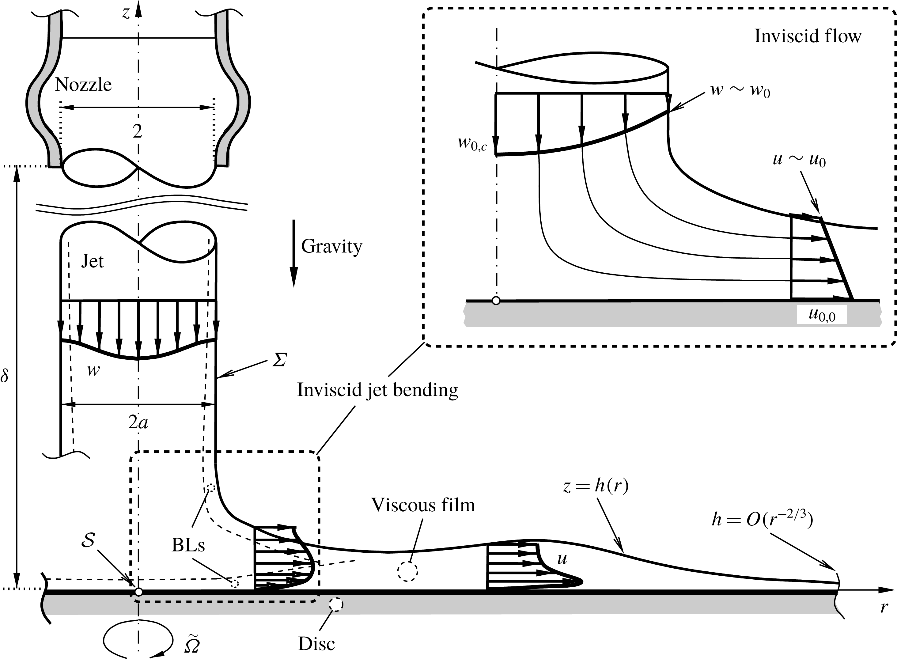
Figure 1. Feasible flow configuration (not to scale, non-dimensional quantities and scalings defined in body text).
Both the considered liquid and the ambient gas are taken as Newtonian, inert and immiscible. Furthermore, the latter is essentially quiescent at zero pressure level and separated from the first by a sharp interface,
 $\unicode[STIX]{x1D6F4}$
. Hereafter, tildes indicate dimensional quantities. Under the isothermal conditions presumed, the liquid (no subscript) and the gaseous environment (subscript
$\unicode[STIX]{x1D6F4}$
. Hereafter, tildes indicate dimensional quantities. Under the isothermal conditions presumed, the liquid (no subscript) and the gaseous environment (subscript
 $e$
) have uniform densities
$e$
) have uniform densities
 $\tilde{\unicode[STIX]{x1D70C}}$
,
$\tilde{\unicode[STIX]{x1D70C}}$
,
 $\tilde{\unicode[STIX]{x1D70C}}_{e}$
, uniform dynamic viscosities
$\tilde{\unicode[STIX]{x1D70C}}_{e}$
, uniform dynamic viscosities
 $\tilde{\unicode[STIX]{x1D707}}$
,
$\tilde{\unicode[STIX]{x1D707}}$
,
 $\tilde{\unicode[STIX]{x1D707}}_{e}$
, hence kinematic ones
$\tilde{\unicode[STIX]{x1D707}}_{e}$
, hence kinematic ones
 $\tilde{\unicode[STIX]{x1D708}}=\tilde{\unicode[STIX]{x1D707}}/\tilde{\unicode[STIX]{x1D70C}}$
,
$\tilde{\unicode[STIX]{x1D708}}=\tilde{\unicode[STIX]{x1D707}}/\tilde{\unicode[STIX]{x1D70C}}$
,
 $\tilde{\unicode[STIX]{x1D708}}_{e}=\tilde{\unicode[STIX]{x1D707}}_{e}/\tilde{\unicode[STIX]{x1D70C}}_{e}$
, and a uniform surface tension
$\tilde{\unicode[STIX]{x1D708}}_{e}=\tilde{\unicode[STIX]{x1D707}}_{e}/\tilde{\unicode[STIX]{x1D70C}}_{e}$
, and a uniform surface tension
 $\tilde{\unicode[STIX]{x1D70E}}$
in
$\tilde{\unicode[STIX]{x1D70E}}$
in
 $\unicode[STIX]{x1D6F4}$
. We anticipate that the reasonable premises
$\unicode[STIX]{x1D6F4}$
. We anticipate that the reasonable premises
 $\tilde{\unicode[STIX]{x1D70C}}/\tilde{\unicode[STIX]{x1D70C}}_{e}\gg 1$
,
$\tilde{\unicode[STIX]{x1D70C}}/\tilde{\unicode[STIX]{x1D70C}}_{e}\gg 1$
,
 $\tilde{\unicode[STIX]{x1D707}}/\tilde{\unicode[STIX]{x1D707}}_{e}\gg 1$
justify the conventional assumption of
$\tilde{\unicode[STIX]{x1D707}}/\tilde{\unicode[STIX]{x1D707}}_{e}\gg 1$
justify the conventional assumption of
 $\unicode[STIX]{x1D6F4}$
being free of normal and viscous tangential stresses, posing the dynamic boundary conditions (BCs). We furthermore introduce the constant gravitational acceleration
$\unicode[STIX]{x1D6F4}$
being free of normal and viscous tangential stresses, posing the dynamic boundary conditions (BCs). We furthermore introduce the constant gravitational acceleration
 $\tilde{g}$
and the constant angular velocity
$\tilde{g}$
and the constant angular velocity
 $\tilde{\unicode[STIX]{x1D6FA}}$
of the disc. Let a nozzle with an orifice of radius
$\tilde{\unicode[STIX]{x1D6FA}}$
of the disc. Let a nozzle with an orifice of radius
 $\tilde{a}$
, positioned a distance
$\tilde{a}$
, positioned a distance
 $\tilde{d}$
above the disc, emit the jet, carrying the volumetric flow rate
$\tilde{d}$
above the disc, emit the jet, carrying the volumetric flow rate
 $\tilde{Q}=\unicode[STIX]{x03C0}\tilde{a}^{2}\tilde{U}$
with the cross-section-averaged speed
$\tilde{Q}=\unicode[STIX]{x03C0}\tilde{a}^{2}\tilde{U}$
with the cross-section-averaged speed
 $\tilde{U}$
at the orifice. Finally,
$\tilde{U}$
at the orifice. Finally,
 $\tilde{r}_{e}$
denotes the disc perimeter and
$\tilde{r}_{e}$
denotes the disc perimeter and
 $\tilde{h}_{e}$
the (suitably controlled) vertical height of the liquid above its edge.
$\tilde{h}_{e}$
the (suitably controlled) vertical height of the liquid above its edge.
2.1 Non-dimensional key groups and orders of magnitude
We conveniently describe the flow in an inertial frame of reference, using polar coordinates
 $r$
,
$r$
,
 $z$
made non-dimensional with
$z$
made non-dimensional with
 $\tilde{a}$
in directions respectively radial from the stagnation point
$\tilde{a}$
in directions respectively radial from the stagnation point
 ${\mathcal{S}}$
, i.e. the centre of rotation, and normal from the wetted face of the disc. Accordingly, let
${\mathcal{S}}$
, i.e. the centre of rotation, and normal from the wetted face of the disc. Accordingly, let
 $u$
,
$u$
,
 $v$
,
$v$
,
 $w$
denote the velocity components, non-dimensional with
$w$
denote the velocity components, non-dimensional with
 $\tilde{U}$
, in the radial, azimuthal and normal directions respectively, and
$\tilde{U}$
, in the radial, azimuthal and normal directions respectively, and
 $p$
the pressure in the flow, non-dimensional with
$p$
the pressure in the flow, non-dimensional with
 $\tilde{\unicode[STIX]{x1D70C}}\tilde{U}^{2}$
. Our focus lies on the flow downstream of jet impingement. Henceforth,
$\tilde{\unicode[STIX]{x1D70C}}\tilde{U}^{2}$
. Our focus lies on the flow downstream of jet impingement. Henceforth,
 $z=h(r)$
rather than its inverse
$z=h(r)$
rather than its inverse
 $r=a(z)$
preferably describes the position of the free surface
$r=a(z)$
preferably describes the position of the free surface
 $\unicode[STIX]{x1D6F4}$
such that
$\unicode[STIX]{x1D6F4}$
such that
 $h$
denotes the local height of the liquid layer and
$h$
denotes the local height of the liquid layer and
 $a$
its local radial extent (double valued due to radial contraction of the freely falling jet).
$a$
its local radial extent (double valued due to radial contraction of the freely falling jet).
Dimensional analysis shows that the sought flow quantities
 $[u,v,w,p](r,z)$
and
$[u,v,w,p](r,z)$
and
 $h(r)$
are parametrised by the complete set of non-dimensional key groups equivalent to the above physical input quantities which characterise the flow:
$h(r)$
are parametrised by the complete set of non-dimensional key groups equivalent to the above physical input quantities which characterise the flow:
 $$\begin{eqnarray}\unicode[STIX]{x1D6FF}:=\tilde{d}/\tilde{a},\quad r_{e}:=\tilde{r}_{e}/\tilde{a},\quad h_{e}:=\tilde{h}_{e}/\tilde{a},\end{eqnarray}$$
 $$\begin{eqnarray}\displaystyle Re_{a}:=\frac{\tilde{U}\tilde{a}}{\tilde{\unicode[STIX]{x1D708}}}=\frac{\tilde{Q}}{\unicode[STIX]{x03C0}\tilde{a}\tilde{\unicode[STIX]{x1D708}}},\quad Ro_{a}:=\frac{\tilde{U}}{\tilde{a}\tilde{\unicode[STIX]{x1D6FA}}}=\frac{\tilde{Q}}{\unicode[STIX]{x03C0}\tilde{a}^{3}\tilde{\unicode[STIX]{x1D6FA}}},\quad Fr_{a}:=\frac{\tilde{U}}{\sqrt{\tilde{g}\tilde{a}}},\quad We_{a}:=\frac{\tilde{\unicode[STIX]{x1D70C}}\tilde{U}^{2}\tilde{a}}{\tilde{\unicode[STIX]{x1D70E}}}. & & \displaystyle \nonumber\\ \displaystyle & & \displaystyle\end{eqnarray}$$
In (2.1d–g
),
 $Re_{a}$
is the Reynolds number formed with the typical jet radius
$Re_{a}$
is the Reynolds number formed with the typical jet radius
 $\tilde{a}$
and characteristic of the internal flow upstream of the nozzle,
$\tilde{a}$
and characteristic of the internal flow upstream of the nozzle,
 $Ro_{a}$
the Rossby number
$Ro_{a}$
the Rossby number
 $Ro_{a}$
measuring the ratio of inertial to centrifugal forces,
$Ro_{a}$
measuring the ratio of inertial to centrifugal forces,
 $Fr_{a}$
the Froude and
$Fr_{a}$
the Froude and
 $We_{a}$
the Weber number, all defined consistently. The associated Bond and capillary numbers
$We_{a}$
the Weber number, all defined consistently. The associated Bond and capillary numbers
 $Bo_{a}=We_{a}/Fr_{a}^{2}$
and
$Bo_{a}=We_{a}/Fr_{a}^{2}$
and
 $Ca_{a}=We_{a}/Re_{a}$
provide useful combinations.
$Ca_{a}=We_{a}/Re_{a}$
provide useful combinations.
The vast majority of applications advocate the usual assumption of a slender free jet and radially spreading film. Moreover, it is realistically accompanied by that of large values of
 $Re_{a}$
:
$Re_{a}$
:
 $$\begin{eqnarray}\unicode[STIX]{x1D6FF}\gg 1,\quad r_{e}\gg 1,\quad Re_{a}\gg 1.\end{eqnarray}$$
Simultaneously,
 $Re_{a}$
is taken as sufficiently small so that laminar–turbulent transition of the flow is expected to occur downstream of any region considered subsequently (a realistic scenario as pointed out by Higuera (Reference Higuera1994)). We add the important restriction
$Re_{a}$
is taken as sufficiently small so that laminar–turbulent transition of the flow is expected to occur downstream of any region considered subsequently (a realistic scenario as pointed out by Higuera (Reference Higuera1994)). We add the important restriction
 $$\begin{eqnarray}Re_{a}/\unicode[STIX]{x1D6FF}\gg 1\end{eqnarray}$$
as this furnishes an appealing possibility to control the behaviour of the jet and, in turn, the film flow (in terms of its purging/etching performances, for instance). The asymptotic analysis will make clear that particular order-of-magnitude requirements for
 $Ro_{a}$
,
$Ro_{a}$
,
 $Fr_{a}$
,
$Fr_{a}$
,
 $We_{a}$
are not as crucial (and can be relaxed) as the fundamental ones in (2.2). Although justified for the majority of potential applications, largeness of
$We_{a}$
are not as crucial (and can be relaxed) as the fundamental ones in (2.2). Although justified for the majority of potential applications, largeness of
 $We_{a}$
, say, does not substantially simplify the treatment of jet deflection where capillary effects are thus kept for the sake of generality (§ 3.2). Most important, assuming formal largeness of
$We_{a}$
, say, does not substantially simplify the treatment of jet deflection where capillary effects are thus kept for the sake of generality (§ 3.2). Most important, assuming formal largeness of
 $Ro_{a}^{2}$
is backed by the scaling of the thin wall-bounded film, associated with a least-degenerate flow description (§ 3.3.1).
$Ro_{a}^{2}$
is backed by the scaling of the thin wall-bounded film, associated with a least-degenerate flow description (§ 3.3.1).
The data of the input quantities listed in table 1 refer to an example typical of genuine application: a liquid/environment constellation water/air at standard conditions. Table 2 displays the values of the corresponding non-dimensional parameters. It is noteworthy that a wide range of species and flow configurations of practical interest give
 $Bo_{a}=O(1)$
and
$Bo_{a}=O(1)$
and
 $Ca_{a}\ll 1$
. In the authors’ opinion, the data in table 1 represent a reliable input for the vast amount of engineering problems. Subsequently, any range of values discussed refers essentially to the variation of
$Ca_{a}\ll 1$
. In the authors’ opinion, the data in table 1 represent a reliable input for the vast amount of engineering problems. Subsequently, any range of values discussed refers essentially to the variation of
 $\tilde{\unicode[STIX]{x1D6FA}}$
in table 1, viz. in table 2 that of
$\tilde{\unicode[STIX]{x1D6FA}}$
in table 1, viz. in table 2 that of
 $Ro_{a}^{2}$
as a key quantity subsequently.
$Ro_{a}^{2}$
as a key quantity subsequently.
Table 1. Typical input values (water jet at
 $20^{\circ }$
,
$20^{\circ }$
,
 $\tilde{U}$
calculated, rounding due to the usual measurements).
$\tilde{U}$
calculated, rounding due to the usual measurements).

Table 2. Values of dimensionless groups according to table 1 (suitably rounded).
It is instructive to first pose the flow problem in full, irrespective of approximations ensuing from the preceding order-of-magnitude estimates.
2.2 Governing equations
The computational domain is fixed by
 $0\leqslant r\leqslant r_{e}$
,
$0\leqslant r\leqslant r_{e}$
,
 $0\leqslant z\leqslant h\leqslant \unicode[STIX]{x1D6FF}$
. As usual, subscripts unambiguously indicate partial derivatives.
$0\leqslant z\leqslant h\leqslant \unicode[STIX]{x1D6FF}$
. As usual, subscripts unambiguously indicate partial derivatives.
The equations of motion comprise the continuity equation
 $$\begin{eqnarray}(ru)_{r}+rw_{z}=0,\end{eqnarray}$$
conveniently satisfied identically through a streamfunction
 $\unicode[STIX]{x1D713}(r,z)$
defined by
$\unicode[STIX]{x1D713}(r,z)$
defined by
 $$\begin{eqnarray}\unicode[STIX]{x1D713}_{z}=ru,\quad \unicode[STIX]{x1D713}_{r}=-rw,\end{eqnarray}$$
and the NSE for, respectively, the radial, azimuthal and vertical directions
 $$\begin{eqnarray}uu_{r}+wu_{z}-v^{2}/r=Re_{a}^{-1}\{[(ru)_{r}/r]_{r}+u_{zz}\}-p_{r},\end{eqnarray}$$
 $$\begin{eqnarray}uv_{r}+wv_{z}+uv/r=Re_{a}^{-1}\{[(rv)_{r}/r]_{r}+v_{zz}\},\end{eqnarray}$$
 $$\begin{eqnarray}uw_{r}+ww_{z}=Re_{a}^{-1}\{(rw_{r})_{r}/r+w_{zz}\}-p_{z}-Fr_{a}^{-2}.\end{eqnarray}$$
The kinematic BCs
 $$\begin{eqnarray}\unicode[STIX]{x1D713}(0,z)=w_{r}(0,z)=0,\quad \unicode[STIX]{x1D713}(r,0)=u(r,0)=0,\quad v(r,0)=rRo_{a}^{-1},\quad \unicode[STIX]{x1D713}(r,h(r))={\textstyle \frac{1}{2}}\end{eqnarray}$$
account for axial symmetry, no penetration and no slip at the disc, and conservation of the volumetric flow rate. Finite disc rotation yields a non-trivial azimuthal flow component
 $v$
above the disc by viscous diffusion, so that (2.5d
) involving the Coriolis acceleration is non-degenerate. The resultant centrifugal body force showing up in (2.5c
) and the mutual coupling of (2.5d
) with (2.5c
) are of specific interest in this study.
$v$
above the disc by viscous diffusion, so that (2.5d
) involving the Coriolis acceleration is non-degenerate. The resultant centrifugal body force showing up in (2.5c
) and the mutual coupling of (2.5d
) with (2.5c
) are of specific interest in this study.
In order to formulate the dynamic BCs, required to determine
 $h(r)$
, we recall the well-known Bonnet expression for the mean curvature
$h(r)$
, we recall the well-known Bonnet expression for the mean curvature
 $$\begin{eqnarray}\unicode[STIX]{x1D705}(r)=-\frac{\text{d}[rh^{\prime }(1+h^{\prime 2})^{-1/2}]/\text{d}r}{2r}=-\frac{h^{\prime }}{2r(1+h^{\prime 2})^{1/2}}-\frac{h^{\prime \prime }}{2(1+h^{\prime 2})^{3/2}}\end{eqnarray}$$
of
 $\unicode[STIX]{x1D6F4}$
and decompose the viscous surface stress, non-dimensional with
$\unicode[STIX]{x1D6F4}$
and decompose the viscous surface stress, non-dimensional with
 $\tilde{\unicode[STIX]{x1D70C}}\tilde{U}^{2}$
, into its tangential components
$\tilde{\unicode[STIX]{x1D70C}}\tilde{U}^{2}$
, into its tangential components
 $\unicode[STIX]{x1D70F}_{m}$
and
$\unicode[STIX]{x1D70F}_{m}$
and
 $\unicode[STIX]{x1D70F}_{a}$
, referring to the median and the azimuthal direction respectively, and its normal component
$\unicode[STIX]{x1D70F}_{a}$
, referring to the median and the azimuthal direction respectively, and its normal component
 $\unicode[STIX]{x1D70F}_{n}$
. This gives
$\unicode[STIX]{x1D70F}_{n}$
. This gives
 $$\begin{eqnarray}Re_{a}(1+h^{\prime 2})\unicode[STIX]{x1D70F}_{m}\equiv [2h^{\prime }(w_{z}-u_{r})+(1-h^{\prime 2})(u_{z}+w_{r})]_{z=h}=0,\end{eqnarray}$$
 $$\begin{eqnarray}Re_{a}(1+h^{\prime 2})^{1/2}\unicode[STIX]{x1D70F}_{a}\equiv [v_{z}-h^{\prime }(v_{r}-v/r)]_{z=h}=0,\end{eqnarray}$$
 $$\begin{eqnarray}\unicode[STIX]{x1D70F}_{n}\equiv \frac{2[h^{\prime 2}u_{r}-h^{\prime }(u_{z}+w_{r})+w_{z}]_{z=h}}{Re_{a}(1+h^{\prime 2})}=p(r,h(r))-\frac{2\unicode[STIX]{x1D705}(r)}{We_{a}}.\end{eqnarray}$$
The following excursus elucidates these zero-stress simplifications, resorting to the estimates stated at the beginning of § 2. The liquid and ambient gaseous phase share the flow speed and the shear stress on their interface
 $\unicode[STIX]{x1D6F4}$
. Then the inertia terms and, in turn, the balanced shear stress gradients in the adjacent liquid shear layer and the relatively thin induced gaseous drag layer are of comparable magnitude. Accordingly,
$\unicode[STIX]{x1D6F4}$
. Then the inertia terms and, in turn, the balanced shear stress gradients in the adjacent liquid shear layer and the relatively thin induced gaseous drag layer are of comparable magnitude. Accordingly,
 $\sqrt{\tilde{\unicode[STIX]{x1D708}}/\tilde{\unicode[STIX]{x1D708}}_{e}}$
measures the ratio of their penetration depths normal to
$\sqrt{\tilde{\unicode[STIX]{x1D708}}/\tilde{\unicode[STIX]{x1D708}}_{e}}$
measures the ratio of their penetration depths normal to
 $\unicode[STIX]{x1D6F4}$
, thus
$\unicode[STIX]{x1D6F4}$
, thus
 $(\tilde{\unicode[STIX]{x1D707}}/\tilde{\unicode[STIX]{x1D707}}_{e})\sqrt{\tilde{\unicode[STIX]{x1D708}}_{e}/\tilde{\unicode[STIX]{x1D708}}}=\sqrt{(\tilde{\unicode[STIX]{x1D70C}}/\tilde{\unicode[STIX]{x1D70C}}_{e})(\tilde{\unicode[STIX]{x1D707}}/\tilde{\unicode[STIX]{x1D707}}_{e})}\gg 1$
that of the shear stresses inside those layers. Equating these when evaluated on
$(\tilde{\unicode[STIX]{x1D707}}/\tilde{\unicode[STIX]{x1D707}}_{e})\sqrt{\tilde{\unicode[STIX]{x1D708}}_{e}/\tilde{\unicode[STIX]{x1D708}}}=\sqrt{(\tilde{\unicode[STIX]{x1D70C}}/\tilde{\unicode[STIX]{x1D70C}}_{e})(\tilde{\unicode[STIX]{x1D707}}/\tilde{\unicode[STIX]{x1D707}}_{e})}\gg 1$
that of the shear stresses inside those layers. Equating these when evaluated on
 $\unicode[STIX]{x1D6F4}$
implies vanishing non-dimensional shear stress as expressed by (2.5k
) and (2.5l
); extending this consideration to the normal-force balance on
$\unicode[STIX]{x1D6F4}$
implies vanishing non-dimensional shear stress as expressed by (2.5k
) and (2.5l
); extending this consideration to the normal-force balance on
 $\unicode[STIX]{x1D6F4}$
leads to (2.5m
).
$\unicode[STIX]{x1D6F4}$
leads to (2.5m
).
The problem is closed once appropriate upstream and downstream conditions are posed. It is reasonable to assume a more-or-less fully developed Hagen–Poiseuille flow in a cylindrical tube ending concentrically in the relatively short, slender nozzle (both having circular cross-sections). It is controlled by the supply and the discharge pressure, the latter given by
 $We_{a}^{-1}$
according to (2.5j
), (2.5m
). By the largeness of
$We_{a}^{-1}$
according to (2.5j
), (2.5m
). By the largeness of
 $Re_{a}$
, the flow undergoes a predominantly inviscid modification inside the nozzle. This raises an idea which might be of interest in engineering applications but, to the authors’ knowledge, is actually not realised so far: as noted above, controlling
$Re_{a}$
, the flow undergoes a predominantly inviscid modification inside the nozzle. This raises an idea which might be of interest in engineering applications but, to the authors’ knowledge, is actually not realised so far: as noted above, controlling
 $w$
and hence the behaviour of the thin radial wall flow can be accomplished via a properly designed axial shape of the nozzle. Its suitably tapered and smooth (polished) inside wall maintains stable laminar flow (cf. McCarthy & Molloy Reference McCarthy and Molloy1974). Specifically, for the sake of simplicity, let its contour exhibit a vertical tangent at the orifice. Then
$w$
and hence the behaviour of the thin radial wall flow can be accomplished via a properly designed axial shape of the nozzle. Its suitably tapered and smooth (polished) inside wall maintains stable laminar flow (cf. McCarthy & Molloy Reference McCarthy and Molloy1974). Specifically, for the sake of simplicity, let its contour exhibit a vertical tangent at the orifice. Then
 $u$
can be considered as negligibly small there, which motivates the model initial conditions (ICs)
$u$
can be considered as negligibly small there, which motivates the model initial conditions (ICs)
 $$\begin{eqnarray}[u,v,w,p](r,\unicode[STIX]{x1D6FF})=[0,0,w_{o}(r),We_{a}^{-1}]\quad (0\leqslant r\leqslant 1),\quad h(1)=\unicode[STIX]{x1D6FF}.\end{eqnarray}$$
Here it is sensible to describe the velocity profile
 $w_{o}(r)$
by a superposition of a typical parabolic profile and a uniform one, accounting for the targeted distortion of the former:
$w_{o}(r)$
by a superposition of a typical parabolic profile and a uniform one, accounting for the targeted distortion of the former:
 $$\begin{eqnarray}w_{o}(r)=2(1-\unicode[STIX]{x1D707})r^{2}-2+\unicode[STIX]{x1D707}\quad ({\leqslant}0,0\leqslant \unicode[STIX]{x1D707}\leqslant 1).\end{eqnarray}$$
The parameter
 $\unicode[STIX]{x1D707}$
specifies variations of the nozzle shape and controls the vorticity introduced under the last condition in (2.5f–i
). The limits
$\unicode[STIX]{x1D707}$
specifies variations of the nozzle shape and controls the vorticity introduced under the last condition in (2.5f–i
). The limits
 $\unicode[STIX]{x1D707}=0$
and
$\unicode[STIX]{x1D707}=0$
and
 $\unicode[STIX]{x1D707}=1$
refer to the full Hagen–Poiseuille and a parallel flow respectively. Notably, the irrotational contribution violates the no-slip condition at the nozzle outlet. However, this is met correctly by a rather steep but smoothing gradient of
$\unicode[STIX]{x1D707}=1$
refer to the full Hagen–Poiseuille and a parallel flow respectively. Notably, the irrotational contribution violates the no-slip condition at the nozzle outlet. However, this is met correctly by a rather steep but smoothing gradient of
 $w_{o}$
as
$w_{o}$
as
 $r\rightarrow 1$
in a BL where
$r\rightarrow 1$
in a BL where
 $1-r=O(Re_{a}^{-1/2})$
originating inside the nozzle. This renders the proposed flow model admissible within our requirements of asymptotic accuracy, given the primarily inviscid flow inside of the nozzle suggested to modify the flow in a supply pipe further upstream. Furthermore, the current deliberate simplification of a one-parametric in lieu of a more involved model of
$1-r=O(Re_{a}^{-1/2})$
originating inside the nozzle. This renders the proposed flow model admissible within our requirements of asymptotic accuracy, given the primarily inviscid flow inside of the nozzle suggested to modify the flow in a supply pipe further upstream. Furthermore, the current deliberate simplification of a one-parametric in lieu of a more involved model of
 $w_{o}(r)$
is acceptable given the possibility of further analytical progress, and the focus of our study. Finally, specifying
$w_{o}(r)$
is acceptable given the possibility of further analytical progress, and the focus of our study. Finally, specifying
 $$\begin{eqnarray}h(r_{e})=h_{e},\end{eqnarray}$$
accommodates the ellipticity of the flow problem. More advanced and physically more meaningful replacements of (2.5p ) are conceivable in the shallow-water limit (cf. Higuera (Reference Higuera1994) and the appendix A).
Also, it proves expedient to identify the components
 $-v_{z}$
,
$-v_{z}$
,
 $u_{z}-w_{r}$
,
$u_{z}-w_{r}$
,
 $(rv)_{r}/r$
of the vorticity for the
$(rv)_{r}/r$
of the vorticity for the
 $r$
-, azimuthal, and
$r$
-, azimuthal, and
 $z$
-direction respectively.
$z$
-direction respectively.
Any attempt to solve the full flow problem governing
 $[\unicode[STIX]{x1D713},v](r,z)$
and the position
$[\unicode[STIX]{x1D713},v](r,z)$
and the position
 $z=h(r)$
of the free surface
$z=h(r)$
of the free surface
 $\unicode[STIX]{x1D6F4}$
as formulated by (2.5p
) numerically requires a major subtleness; at least to the extent of the desired grade of resolution. Specifically the better the restriction (2.3) is satisfied, the more calculating the position of
$\unicode[STIX]{x1D6F4}$
as formulated by (2.5p
) numerically requires a major subtleness; at least to the extent of the desired grade of resolution. Specifically the better the restriction (2.3) is satisfied, the more calculating the position of
 $\unicode[STIX]{x1D6F4}$
with satisfactory accuracy is compromised. This becomes obvious from the slenderness of both the jet and the resultant radially spreading film; the first associated with viscous forces acting in the aforementioned rather slowly growing thin sublayers along
$\unicode[STIX]{x1D6F4}$
with satisfactory accuracy is compromised. This becomes obvious from the slenderness of both the jet and the resultant radially spreading film; the first associated with viscous forces acting in the aforementioned rather slowly growing thin sublayers along
 $\unicode[STIX]{x1D6F4}$
, the second with a complex interplay of viscous and centrifugal forces. This without doubt renders the problem an intriguing one. Consequently, resolving the richness of interesting flow details is not routine. In fact, it has not been accomplished so far. These assessments strongly substantiate the need for asymptotic techniques. A systematic reduction process then obviates the need of a multiparametric, full numerical study of (2.5p
). The so obtained much more feasible one highlights all the features of the film flow on the conditions (2.2) and (2.3) at drastically reduced computational costs and under variation of only a few similarity parameters (§ 4). Most important, the achieved parabolicity of the leading-order problem makes (2.5p
) ultimately obsolete by suppressing the difficile upstream influence by
$\unicode[STIX]{x1D6F4}$
, the second with a complex interplay of viscous and centrifugal forces. This without doubt renders the problem an intriguing one. Consequently, resolving the richness of interesting flow details is not routine. In fact, it has not been accomplished so far. These assessments strongly substantiate the need for asymptotic techniques. A systematic reduction process then obviates the need of a multiparametric, full numerical study of (2.5p
). The so obtained much more feasible one highlights all the features of the film flow on the conditions (2.2) and (2.3) at drastically reduced computational costs and under variation of only a few similarity parameters (§ 4). Most important, the achieved parabolicity of the leading-order problem makes (2.5p
) ultimately obsolete by suppressing the difficile upstream influence by
 $r_{e}$
,
$r_{e}$
,
 $h_{e}$
in (2.1a–c
).
$h_{e}$
in (2.1a–c
).
3 Asymptotic structure of the flow
We proceed by elucidating four flow regions to be distinguished grossly: the jet exiting the nozzle and then freely falling (§ 3.1); that of its bending due to its impingement (§ 3.2); the thin viscous BL forming adjacent to the disc (§ 3.3); the relatively thin, radially spreading developed film (a notion here preferred against the common ‘wall jet’, used later for a submerged jet), where viscous effects are finally of importance across its whole thickness (§ 3.4).
3.1 Jet regime:
 $r=O(1)$
,
$h\gg 1$
$r=O(1)$
,
$h\gg 1$


We first make reference to the earlier discussion of the radial distribution of
 $w$
and an associated thin edge layer. Initially,
$w$
and an associated thin edge layer. Initially,
 $w\sim w_{o}$
given by (2.5o
) holds in the bulk of the just forming jet where
$w\sim w_{o}$
given by (2.5o
) holds in the bulk of the just forming jet where
 $a-r$
is not too small; in the second viscosity regularises (for any value of
$a-r$
is not too small; in the second viscosity regularises (for any value of
 $Re_{a}$
) the jump at the orifice from a no-slip towards a free-slip condition (or
$Re_{a}$
) the jump at the orifice from a no-slip towards a free-slip condition (or
 $w=O(a-r)$
to
$w=O(a-r)$
to
 $w_{r}=O(a-r)$
as
$w_{r}=O(a-r)$
as
 $r\rightarrow a$
). The latter follows from (2.5k
) in the ‘jet limit’
$r\rightarrow a$
). The latter follows from (2.5k
) in the ‘jet limit’
 $h^{\prime }\rightarrow -\infty$
.
$h^{\prime }\rightarrow -\infty$
.
For any howsoever small initial surface slip
 $\unicode[STIX]{x1D707}>0$
, Khayat (Reference Khayat2016) aids in describing the non-trivial local modification of the aforementioned shear layer. If
$\unicode[STIX]{x1D707}>0$
, Khayat (Reference Khayat2016) aids in describing the non-trivial local modification of the aforementioned shear layer. If
 $\unicode[STIX]{x1D707}=0$
, the findings by Khayat (Reference Khayat2017) and the regularisation of the Goldstein singularity by localised viscous–inviscid interaction of the type put forward by Scheichl, Bowles & Pasias (Reference Scheichl, Bowles and Pasias2018) apply. Since vertical convection balances viscous diffusion in that edge layer, inspection analysis of (2.5e
) yields the order-of-magnitude estimates
$\unicode[STIX]{x1D707}=0$
, the findings by Khayat (Reference Khayat2017) and the regularisation of the Goldstein singularity by localised viscous–inviscid interaction of the type put forward by Scheichl, Bowles & Pasias (Reference Scheichl, Bowles and Pasias2018) apply. Since vertical convection balances viscous diffusion in that edge layer, inspection analysis of (2.5e
) yields the order-of-magnitude estimates
 $w\sim a-r$
, by (2.5o
), and
$w\sim a-r$
, by (2.5o
), and
 $w^{2}/(\unicode[STIX]{x1D6FF}-z)\sim w/[Re_{a}(a-r)^{2}]$
there. One then typically locates its formation immediately downstream of interaction for
$w^{2}/(\unicode[STIX]{x1D6FF}-z)\sim w/[Re_{a}(a-r)^{2}]$
there. One then typically locates its formation immediately downstream of interaction for
 $$\begin{eqnarray}\unicode[STIX]{x1D707}=0:\quad (a-r)^{3}\sim (1-\breve{z})\unicode[STIX]{x1D6FF}/Re_{a}\ll 1,\quad \breve{z}:=z/\unicode[STIX]{x1D6FF}.\end{eqnarray}$$
Slenderness of the bulk region of the jet implies
 $u=O(\unicode[STIX]{x1D6FF}^{-1})$
via (2.4) and (2.5o
) and
$u=O(\unicode[STIX]{x1D6FF}^{-1})$
via (2.4) and (2.5o
) and
 $p\sim (We_{a}\,a)^{-1}+O(\unicode[STIX]{x1D6FF}^{-2})$
according to (2.5m
) and (2.5c
). To confirm the previous and subsequent scalings as adequate for the targeted flow control, let us first elucidate the flow in a least-degenerate fashion. To this end, we relax (2.3) and take
$p\sim (We_{a}\,a)^{-1}+O(\unicode[STIX]{x1D6FF}^{-2})$
according to (2.5m
) and (2.5c
). To confirm the previous and subsequent scalings as adequate for the targeted flow control, let us first elucidate the flow in a least-degenerate fashion. To this end, we relax (2.3) and take
 $Re_{a}/\unicode[STIX]{x1D6FF}$
but also
$Re_{a}/\unicode[STIX]{x1D6FF}$
but also
 $We_{a}$
as of
$We_{a}$
as of
 $O(1)$
. This fastens the merging of the edge BL and the bulk layer by viscous diffusion. There the one-term expansions
$O(1)$
. This fastens the merging of the edge BL and the bulk layer by viscous diffusion. There the one-term expansions
 $\unicode[STIX]{x1D713}\sim \breve{\unicode[STIX]{x1D713}}(r,\breve{z})$
,
$\unicode[STIX]{x1D713}\sim \breve{\unicode[STIX]{x1D713}}(r,\breve{z})$
,
 $w\sim \breve{w}=-\breve{\unicode[STIX]{x1D713}}_{r}/r$
,
$w\sim \breve{w}=-\breve{\unicode[STIX]{x1D713}}_{r}/r$
,
 $a\sim \breve{a}(\breve{z})$
(
$a\sim \breve{a}(\breve{z})$
(
 $\breve{z}=O(1)$
,
$\breve{z}=O(1)$
,
 $\unicode[STIX]{x1D6FF}\gg 1$
) and (2.5a,b
) yield the shear-layer approximation
$\unicode[STIX]{x1D6FF}\gg 1$
) and (2.5a,b
) yield the shear-layer approximation
 $$\begin{eqnarray}\breve{\unicode[STIX]{x1D713}}_{r}\breve{\unicode[STIX]{x1D713}}_{r\breve{z}}-\breve{\unicode[STIX]{x1D713}}_{\breve{z}}\breve{\unicode[STIX]{x1D713}}_{rr}+\breve{\unicode[STIX]{x1D713}}_{\breve{z}}\breve{\unicode[STIX]{x1D713}}_{r}/r=-r^{2}\breve{p}^{\prime }(\breve{z})-(\unicode[STIX]{x1D6FF}/Re_{a})r[r(\breve{\unicode[STIX]{x1D713}}_{r}/r)_{r}]_{r}\end{eqnarray}$$
of (2.5e
) with the suitably reduced pressure, zero at the nozzle exit (
 $\breve{z}=1$
),
$\breve{z}=1$
),
 $$\begin{eqnarray}\breve{p}(\breve{z}):=Fr_{d}^{-2}(\breve{z}-1)+We_{a}^{-1}(\breve{a}^{-1}-1),\quad Fr_{d}:=Fr_{a}/\sqrt{\unicode[STIX]{x1D6FF}}.\end{eqnarray}$$
For the resulting typical value of the Froude number
 $Fr_{d}$
formed with the height of fall
$Fr_{d}$
formed with the height of fall
 $\tilde{d}$
see table 2. Equation (3.2a
) is then subject to the ICs and kinematic BCs
$\tilde{d}$
see table 2. Equation (3.2a
) is then subject to the ICs and kinematic BCs
 $$\begin{eqnarray}[(\breve{\unicode[STIX]{x1D713}}_{r}/r)(r,1),\breve{a}(1)]=[-w_{o}(r),1],\quad [\breve{\unicode[STIX]{x1D713}},(\breve{\unicode[STIX]{x1D713}}_{r}/r)_{r}](0,\breve{z})=[0,0],\breve{\unicode[STIX]{x1D713}}(\breve{a},\breve{z})={\textstyle \frac{1}{2}},\end{eqnarray}$$
cf. (2.5n ), (2.5o ) and (2.5f–i ) respectively, and the free-slip condition
 $$\begin{eqnarray}(\breve{\unicode[STIX]{x1D713}}_{r}/r)_{r}(\breve{a},\breve{z})=0\end{eqnarray}$$
provided by (2.5k
). Owing to the lack of a symmetry-breaking no-slip condition, the BL problem (3.2) governing
 $\breve{\unicode[STIX]{x1D713}}$
and
$\breve{\unicode[STIX]{x1D713}}$
and
 $\breve{a}$
, as entering the sought pressure contribution, for
$\breve{a}$
, as entering the sought pressure contribution, for
 $0\leqslant r\leqslant \breve{a}$
,
$0\leqslant r\leqslant \breve{a}$
,
 $0<\breve{z}\leqslant 1$
is of parabolic type. That is, the jet does not ‘feel’ a feedback of its impact in the leading approximation: consequently, stopping the (numerical) downstream integration of (3.2) for
$0<\breve{z}\leqslant 1$
is of parabolic type. That is, the jet does not ‘feel’ a feedback of its impact in the leading approximation: consequently, stopping the (numerical) downstream integration of (3.2) for
 $\breve{z}=0$
yields the terminal jet contraction
$\breve{z}=0$
yields the terminal jet contraction
 $a_{0}:=\breve{a}(0)$
and
$a_{0}:=\breve{a}(0)$
and
 $\breve{w}$
-profile
$\breve{w}$
-profile
 $w_{0}(r):=\breve{w}(r,0)$
. For more interesting details see Tillett (Reference Tillett1968).
$w_{0}(r):=\breve{w}(r,0)$
. For more interesting details see Tillett (Reference Tillett1968).
The assumption (2.3) ensures a predominantly inviscid and yet swirl-free (
 $v\sim 0$
)
$v\sim 0$
)
 $90^{\circ }$
-deflection of the flow where
$90^{\circ }$
-deflection of the flow where
 $r,z=O(a_{0})$
and the jet approximation breaks down. By the largeness of
$r,z=O(a_{0})$
and the jet approximation breaks down. By the largeness of
 $Re_{a}$
, the spin of the disc is indeed noticeable only via (2.5f–i
) in an adjacent BL, typically having a vertical extent not larger than of
$Re_{a}$
, the spin of the disc is indeed noticeable only via (2.5f–i
) in an adjacent BL, typically having a vertical extent not larger than of
 $O(Re_{a}^{-1/2})$
even for arbitrarily small values of
$O(Re_{a}^{-1/2})$
even for arbitrarily small values of
 $Ro_{a}$
. This scenario is investigated in § 3.3. It alleviates drastically the prediction of the modification of the initial
$Ro_{a}$
. This scenario is investigated in § 3.3. It alleviates drastically the prediction of the modification of the initial
 $w$
-profile in the nozzle and thus the control of the
$w$
-profile in the nozzle and thus the control of the
 $u$
-profile in the developed film (for etching/cleaning purposes). Assuming a fully viscous falling jet, however, requires the numerical solution of (3.2) and a systematic variation of
$u$
-profile in the developed film (for etching/cleaning purposes). Assuming a fully viscous falling jet, however, requires the numerical solution of (3.2) and a systematic variation of
 $\unicode[STIX]{x1D6FF}/Re_{a}$
,
$\unicode[STIX]{x1D6FF}/Re_{a}$
,
 $Fr_{d}$
,
$Fr_{d}$
,
 $We_{a}$
and
$We_{a}$
and
 $\unicode[STIX]{x1D707}$
. That is, as long as (2.3) is not met, a desirable simplification arises only if
$\unicode[STIX]{x1D707}$
. That is, as long as (2.3) is not met, a desirable simplification arises only if
 $Fr_{d}$
is small, i.e.
$Fr_{d}$
is small, i.e.
 $\tilde{d}$
chosen as correspondingly large, since the viscous term in (3.2a
) is predominant only for
$\tilde{d}$
chosen as correspondingly large, since the viscous term in (3.2a
) is predominant only for
 $\breve{z}=O(Fr_{d}^{2})$
. For larger values of
$\breve{z}=O(Fr_{d}^{2})$
. For larger values of
 $\breve{z}$
, the increasing action of gravity and the absence of external shear forces accelerate the jet whereas vorticity is no longer diffused, and inspection of (3.2) recovers Toricelli’s law for uniform flow and the associated jet thinning:
$\breve{z}$
, the increasing action of gravity and the absence of external shear forces accelerate the jet whereas vorticity is no longer diffused, and inspection of (3.2) recovers Toricelli’s law for uniform flow and the associated jet thinning:
 $$\begin{eqnarray}\breve{w}\sim -\sqrt{2(1-\breve{z})}/Fr_{d},\quad \breve{a}\sim 1/\sqrt{-\breve{w}}.\end{eqnarray}$$
(This scenario applies even for only moderately large values of
 $Re_{a}$
: then the viscous and, by (3.2c,d
), also the convective terms dominate (3.2a
) already for smaller values of
$Re_{a}$
: then the viscous and, by (3.2c,d
), also the convective terms dominate (3.2a
) already for smaller values of
 $\breve{z}$
before gravity becomes important, which finally confirms the above results further downstream.)
$\breve{z}$
before gravity becomes important, which finally confirms the above results further downstream.)
The marked increase of the irrotational contribution to
 $w$
by (3.3) also hampers severely the desired control of the vorticity. Hence, the demand for a viable control strategy underpins the requirement (2.3), i.e. of a predominantly inviscid fall of the jet already for
$w$
by (3.3) also hampers severely the desired control of the vorticity. Hence, the demand for a viable control strategy underpins the requirement (2.3), i.e. of a predominantly inviscid fall of the jet already for
 $\breve{z}=O(1)$
. Then the viscous term in (3.2a
) remains small, thus the edge BL slender and of a thickness
$\breve{z}=O(1)$
. Then the viscous term in (3.2a
) remains small, thus the edge BL slender and of a thickness
 $\unicode[STIX]{x1D6E5}:=\sqrt{\unicode[STIX]{x1D6FF}/Re_{a}}$
, see figure 1. In this inviscid-flow limit, the expensive systematic numerical investigation of the full problem (3.2) is superseded by the analytical evaluation of its first integral. This expresses Bernoulli’s theorem in von Mises form:
$\unicode[STIX]{x1D6E5}:=\sqrt{\unicode[STIX]{x1D6FF}/Re_{a}}$
, see figure 1. In this inviscid-flow limit, the expensive systematic numerical investigation of the full problem (3.2) is superseded by the analytical evaluation of its first integral. This expresses Bernoulli’s theorem in von Mises form:
 $\breve{w}=-\sqrt{w_{o}^{2}-2\breve{p}}$
is a function of
$\breve{w}=-\sqrt{w_{o}^{2}-2\breve{p}}$
is a function of
 $\breve{\unicode[STIX]{x1D713}}$
and
$\breve{\unicode[STIX]{x1D713}}$
and
 $\breve{z}$
. Integrating
$\breve{z}$
. Integrating
 $r\breve{w}=-\breve{\unicode[STIX]{x1D713}}_{r}$
for
$r\breve{w}=-\breve{\unicode[STIX]{x1D713}}_{r}$
for
 $\breve{z}=1$
reveals
$\breve{z}=1$
reveals
 $w_{o}=-\sqrt{(2-\unicode[STIX]{x1D707})^{2}-8(1-\unicode[STIX]{x1D707})\breve{\unicode[STIX]{x1D713}}}$
, according to (3.2c,d
) and (2.5o
), and once again for
$w_{o}=-\sqrt{(2-\unicode[STIX]{x1D707})^{2}-8(1-\unicode[STIX]{x1D707})\breve{\unicode[STIX]{x1D713}}}$
, according to (3.2c,d
) and (2.5o
), and once again for
 $\breve{z}\leqslant 1$
subject to (3.2c,d
) preservation of vorticity along streamlines:
$\breve{z}\leqslant 1$
subject to (3.2c,d
) preservation of vorticity along streamlines:
 $$\begin{eqnarray}\displaystyle & \breve{\unicode[STIX]{x1D713}}=(\unicode[STIX]{x1D707}-1)r^{4}/2-\breve{w}_{c}(\breve{z})r^{2}/2,\quad \breve{w}_{c}(\breve{z}):=-\sqrt{(2-\unicode[STIX]{x1D707})^{2}-2\breve{p}(\breve{z})}, & \displaystyle\end{eqnarray}$$
 $$\begin{eqnarray}\displaystyle & \breve{w}=-\sqrt{(2-\unicode[STIX]{x1D707})^{2}-2\breve{p}-8(1-\unicode[STIX]{x1D707})\breve{\unicode[STIX]{x1D713}}}=2(1-\unicode[STIX]{x1D707})r^{2}+\breve{w}_{c}(\breve{z})\quad (0\leqslant r\leqslant \breve{a}).\qquad & \displaystyle\end{eqnarray}$$
 $\breve{w}_{c}$
is the flow speed along the jet centreline. Substituting the last of the conditions (3.2c,d
) into (3.4a
) and (3.2b
) gives for
$\breve{w}_{c}$
is the flow speed along the jet centreline. Substituting the last of the conditions (3.2c,d
) into (3.4a
) and (3.2b
) gives for
 $We_{a}<\infty$
(
$We_{a}<\infty$
(
 $We_{a}=\infty$
) an implicit (explicit) expression for the local jet contraction
$We_{a}=\infty$
) an implicit (explicit) expression for the local jet contraction
 $\breve{a}$
, effectively as a function of
$\breve{a}$
, effectively as a function of  $$\begin{eqnarray}\unicode[STIX]{x1D6EC}(\breve{z}):=Fr_{d}^{-2}(1-\breve{z})+We_{a}^{-1}=(We_{a}\breve{a})^{-1}-\breve{p}(\breve{z}),\end{eqnarray}$$
 $We_{a}$
(cf. Gurevich Reference Gurevich1961), and
$We_{a}$
(cf. Gurevich Reference Gurevich1961), and
 $1-\unicode[STIX]{x1D707}$
as a measure of the vorticity. It is advantageously written as
$1-\unicode[STIX]{x1D707}$
as a measure of the vorticity. It is advantageously written as
 $$\begin{eqnarray}[\breve{a}^{-2}+(1-\unicode[STIX]{x1D707})\breve{a}^{2}]^{2}=\breve{w}_{c}^{2}=2\unicode[STIX]{x1D6EC}-2(We_{a}\breve{a})^{-1}+(2-\unicode[STIX]{x1D707})^{2}.\end{eqnarray}$$
This finally yields the flow factors
 $a_{0}$
and
$a_{0}$
and
 $w_{0,c}:=\breve{w}_{c}(0)$
by (3.4a
) and (3.5), providing the match with the flows in the jet and the region of its marked deflection.
$w_{0,c}:=\breve{w}_{c}(0)$
by (3.4a
) and (3.5), providing the match with the flows in the jet and the region of its marked deflection.
For the distributions of
 $\breve{a}$
and
$\breve{a}$
and
 $\breve{w}_{c}$
see figure 2. Here varying
$\breve{w}_{c}$
see figure 2. Here varying
 $\unicode[STIX]{x1D707}$
has only little effect; according to table 3, with
$\unicode[STIX]{x1D707}$
has only little effect; according to table 3, with
 $$\begin{eqnarray}\unicode[STIX]{x1D6EC}_{0}:=\unicode[STIX]{x1D6EC}(0)=Fr_{d}^{-2}+We_{a}^{-1}\end{eqnarray}$$
and the typical data for these two addends, a rather moderate end contraction rate
 $a_{0}$
ensues. In general,
$a_{0}$
ensues. In general,
 $0<\breve{a}\leqslant 1$
holds, and
$0<\breve{a}\leqslant 1$
holds, and
 $\breve{a}$
decreases as
$\breve{a}$
decreases as
 $\breve{z}$
,
$\breve{z}$
,
 $Fr_{d}^{-1}$
,
$Fr_{d}^{-1}$
,
 $We_{a}^{-1}$
,
$We_{a}^{-1}$
,
 $\unicode[STIX]{x1D707}$
decrease. Thus,
$\unicode[STIX]{x1D707}$
decrease. Thus,
 $a_{0}$
becomes quite small for a very slender jet, elongated by gravity, eventually in the asymptotic limit (3.3) implied by (3.4b
), (3.6) and (3.2b
). The behaviour of
$a_{0}$
becomes quite small for a very slender jet, elongated by gravity, eventually in the asymptotic limit (3.3) implied by (3.4b
), (3.6) and (3.2b
). The behaviour of
 $\breve{w}_{c}$
turns out to be strictly reciprocal. We note that jet formation at the nozzle exit is governed by the limit
$\breve{w}_{c}$
turns out to be strictly reciprocal. We note that jet formation at the nozzle exit is governed by the limit
 $\unicode[STIX]{x1D706}:=\unicode[STIX]{x1D6EC}-We_{a}^{-1}\rightarrow 0_{+}$
. In turn, setting
$\unicode[STIX]{x1D706}:=\unicode[STIX]{x1D6EC}-We_{a}^{-1}\rightarrow 0_{+}$
. In turn, setting
 $\unicode[STIX]{x1D6FE}:=1-\breve{a}$
gives
$\unicode[STIX]{x1D6FE}:=1-\breve{a}$
gives
 $\breve{p}\sim -\unicode[STIX]{x1D706}+We_{a}^{-1}[\unicode[STIX]{x1D6FE}+\unicode[STIX]{x1D6FE}^{2}+O(\unicode[STIX]{x1D6FE}^{3})]$
where
$\breve{p}\sim -\unicode[STIX]{x1D706}+We_{a}^{-1}[\unicode[STIX]{x1D6FE}+\unicode[STIX]{x1D6FE}^{2}+O(\unicode[STIX]{x1D6FE}^{3})]$
where
 $\unicode[STIX]{x1D6FE}$
expands in three different forms:
$\unicode[STIX]{x1D6FE}$
expands in three different forms:
 $\unicode[STIX]{x1D6FE}\sim [We_{a}^{-1}+2\unicode[STIX]{x1D707}(2-\unicode[STIX]{x1D707})]\unicode[STIX]{x1D706}+O(\unicode[STIX]{x1D706}^{2})$
(
$\unicode[STIX]{x1D6FE}\sim [We_{a}^{-1}+2\unicode[STIX]{x1D707}(2-\unicode[STIX]{x1D707})]\unicode[STIX]{x1D706}+O(\unicode[STIX]{x1D706}^{2})$
(
 $\unicode[STIX]{x1D707}>0$
);
$\unicode[STIX]{x1D707}>0$
);
 $\unicode[STIX]{x1D6FE}\sim \sqrt{\unicode[STIX]{x1D706}/8}+O(\unicode[STIX]{x1D706})$
(
$\unicode[STIX]{x1D6FE}\sim \sqrt{\unicode[STIX]{x1D706}/8}+O(\unicode[STIX]{x1D706})$
(
 $\unicode[STIX]{x1D707}=We_{a}^{-1}=0$
);
$\unicode[STIX]{x1D707}=We_{a}^{-1}=0$
);
 $\unicode[STIX]{x1D6FE}\sim We_{a}\unicode[STIX]{x1D706}-We_{a}^{2}(8We_{a}^{-1}+1)\unicode[STIX]{x1D706}^{2}+O(\unicode[STIX]{x1D706}^{3})$
(
$\unicode[STIX]{x1D6FE}\sim We_{a}\unicode[STIX]{x1D706}-We_{a}^{2}(8We_{a}^{-1}+1)\unicode[STIX]{x1D706}^{2}+O(\unicode[STIX]{x1D706}^{3})$
(
 $\unicode[STIX]{x1D707}=0$
,
$\unicode[STIX]{x1D707}=0$
,
 $We_{a}<\infty$
). Here the first two imply
$We_{a}<\infty$
). Here the first two imply
 $\breve{w}_{c}\sim -(2-\unicode[STIX]{x1D707})+O(\unicode[STIX]{x1D706})$
, the second an irregular sudden expansion of the jet (smoothed out by surface tension,
$\breve{w}_{c}\sim -(2-\unicode[STIX]{x1D707})+O(\unicode[STIX]{x1D706})$
, the second an irregular sudden expansion of the jet (smoothed out by surface tension,
 $We_{a}\gg 1$
) and the last
$We_{a}\gg 1$
) and the last
 $\breve{w}_{c}\sim -(2-\unicode[STIX]{x1D707})-16(We_{a}\unicode[STIX]{x1D706})^{2}/(2-\unicode[STIX]{x1D707})+O(\unicode[STIX]{x1D706}^{3})$
. As for what follows, even more important, we also find the behaviour
$\breve{w}_{c}\sim -(2-\unicode[STIX]{x1D707})-16(We_{a}\unicode[STIX]{x1D706})^{2}/(2-\unicode[STIX]{x1D707})+O(\unicode[STIX]{x1D706}^{3})$
. As for what follows, even more important, we also find the behaviour
 $$\begin{eqnarray}[\breve{a},\breve{w}_{c}]\sim [(2\unicode[STIX]{x1D6EC})^{-1/4},\,-(2\unicode[STIX]{x1D6EC})^{1/2}]+O([\unicode[STIX]{x1D6EC}^{-9/4},\unicode[STIX]{x1D6EC}^{-1/2}][1+We_{a}^{-1}\unicode[STIX]{x1D6EC}^{1/4}])\quad (\unicode[STIX]{x1D6EC}\gg 1).\end{eqnarray}$$
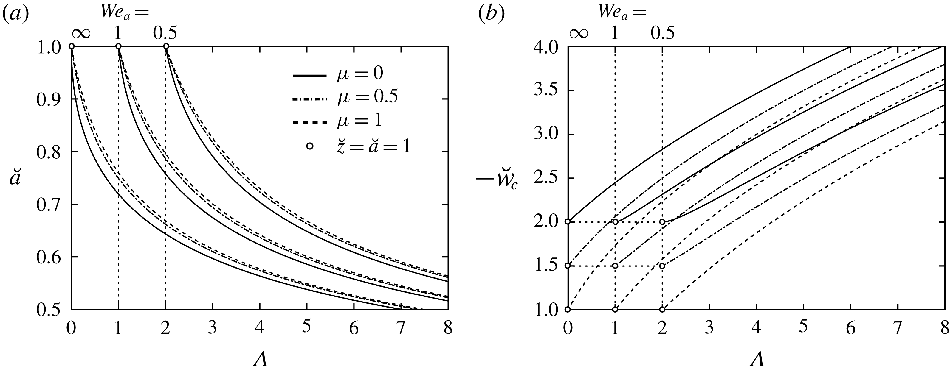
Figure 2. Jet contraction
 $\breve{a}$
(a) and centre speed
$\breve{a}$
(a) and centre speed
 $\breve{w}_{c}$
(b) by varying
$\breve{w}_{c}$
(b) by varying
 $\unicode[STIX]{x1D6EC}$
,
$\unicode[STIX]{x1D6EC}$
,
 $We_{a}$
,
$We_{a}$
,
 $\unicode[STIX]{x1D707}$
(same legend).
$\unicode[STIX]{x1D707}$
(same legend).
Table 3. Characteristic values governing jet deflection and the thin film according to table 2.
The parabolic contribution to
 $\breve{w}$
scales with
$\breve{w}$
scales with
 $\breve{a}^{2}$
but the irrotational one
$\breve{a}^{2}$
but the irrotational one
 $\breve{w}_{c}$
with
$\breve{w}_{c}$
with
 $\breve{a}^{-2}$
. We hence consider the characteristic flow speed
$\breve{a}^{-2}$
. We hence consider the characteristic flow speed
 $\tilde{U}_{0}:=\tilde{U}/a_{0}^{2}$
and jet radius
$\tilde{U}_{0}:=\tilde{U}/a_{0}^{2}$
and jet radius
 $\tilde{a}_{0}:=a_{0}\tilde{a}$
in the region of pronounced jet deflection
$\tilde{a}_{0}:=a_{0}\tilde{a}$
in the region of pronounced jet deflection
 $z=O(a_{0})$
, with (3.3) providing a lower bound for
$z=O(a_{0})$
, with (3.3) providing a lower bound for
 $a_{0}$
. In turn, adequately defined Froude, Reynolds and Weber numbers are
$a_{0}$
. In turn, adequately defined Froude, Reynolds and Weber numbers are
 $$\begin{eqnarray}Fr_{0}:=\tilde{U}_{0}/\sqrt{\tilde{g}\tilde{a}_{0}}=Fr_{a}/a_{0}^{5/2},\quad Re_{0}:=Re_{a}/a_{0},\quad We_{0}:=We_{a}/a_{0}^{3}.\end{eqnarray}$$
The premise (2.3) renders (3.3) valid for
 $Fr_{d}\ll 1$
in (3.2b
), which implies
$Fr_{d}\ll 1$
in (3.2b
), which implies
 $\unicode[STIX]{x1D6EC}\sim Fr_{d}^{-2}$
and
$\unicode[STIX]{x1D6EC}\sim Fr_{d}^{-2}$
and
 $a_{0}\sim Fr_{d}^{1/2}/2^{1/4}$
per (3.5) and (3.8), hence
$a_{0}\sim Fr_{d}^{1/2}/2^{1/4}$
per (3.5) and (3.8), hence
 $Fr_{0}/Fr_{a}\sim 2^{5/8}/Fr_{d}^{5/4}=(2\unicode[STIX]{x1D6FF})^{5/8}/Fr_{a}^{5/4}$
. The values in table 2 also imply
$Fr_{0}/Fr_{a}\sim 2^{5/8}/Fr_{d}^{5/4}=(2\unicode[STIX]{x1D6FF})^{5/8}/Fr_{a}^{5/4}$
. The values in table 2 also imply
 $Fr_{0}\gg 1$
, but rather due to the largeness of
$Fr_{0}\gg 1$
, but rather due to the largeness of
 $Fr_{a}$
than the smallness of
$Fr_{a}$
than the smallness of
 $Fr_{d}$
. The latter is argued by Higuera (Reference Higuera1994, p. 72, bottom) when he claims that ‘
$Fr_{d}$
. The latter is argued by Higuera (Reference Higuera1994, p. 72, bottom) when he claims that ‘
 $\tilde{U}_{0}^{2}/(2\tilde{g})$
is the head of the fluid in the jet, typically large compared with its half-width
$\tilde{U}_{0}^{2}/(2\tilde{g})$
is the head of the fluid in the jet, typically large compared with its half-width
 $a_{0}$
’ (our notations used) – which means
$a_{0}$
’ (our notations used) – which means
 $Fr_{0}\gg 1$
finally. The present view agrees on neglecting the effect of gravity on jet bending but sees it only moderately increasing
$Fr_{0}\gg 1$
finally. The present view agrees on neglecting the effect of gravity on jet bending but sees it only moderately increasing
 $\breve{w}_{c}$
and decreasing
$\breve{w}_{c}$
and decreasing
 $a_{0}$
as
$a_{0}$
as
 $Fr_{d}$
is considered to take on rather not so small corresponding values. In the irrotational-flow limit
$Fr_{d}$
is considered to take on rather not so small corresponding values. In the irrotational-flow limit
 $\unicode[STIX]{x1D707}\rightarrow 1_{-}$
, one also confirms
$\unicode[STIX]{x1D707}\rightarrow 1_{-}$
, one also confirms
 $a_{0}=O(1)$
for
$a_{0}=O(1)$
for
 $\breve{w}\sim \breve{w}_{c}$
and again
$\breve{w}\sim \breve{w}_{c}$
and again
 $\breve{a}\sim 1/\sqrt{-\breve{w}}=1/[1+2\unicode[STIX]{x1D6EC}-2/(We_{a}\breve{a})]^{1/4}$
(cf. figure 2), but now holding for the more realistic, moderate values of
$\breve{a}\sim 1/\sqrt{-\breve{w}}=1/[1+2\unicode[STIX]{x1D6EC}-2/(We_{a}\breve{a})]^{1/4}$
(cf. figure 2), but now holding for the more realistic, moderate values of
 $Fr_{d}$
. However, in the following
$Fr_{d}$
. However, in the following
 $Fr_{d}$
and thus
$Fr_{d}$
and thus
 $a_{0}$
are allowed to become very small. Therefore, taking
$a_{0}$
are allowed to become very small. Therefore, taking
 $\tilde{a}_{0}$
as the new length scale representative of jet impingement includes this case conveniently.
$\tilde{a}_{0}$
as the new length scale representative of jet impingement includes this case conveniently.
With (3.2a
), (3.2c,d
) and (3.2e
), we now may also be more specific as to the viscous perturbations of
 $\breve{\unicode[STIX]{x1D713}}$
and hence the surface slip
$\breve{\unicode[STIX]{x1D713}}$
and hence the surface slip
 $W(\breve{z}):=-\breve{w}(\breve{a},\breve{z})\;({>}0)$
by the edge shear layer. There
$W(\breve{z}):=-\breve{w}(\breve{a},\breve{z})\;({>}0)$
by the edge shear layer. There
 $\unicode[STIX]{x1D713}\sim 1/2-\unicode[STIX]{x1D6E5}W+\unicode[STIX]{x1D6E5}^{2}\unicode[STIX]{x1D6F9}(\breve{R},\breve{z})$
where
$\unicode[STIX]{x1D713}\sim 1/2-\unicode[STIX]{x1D6E5}W+\unicode[STIX]{x1D6E5}^{2}\unicode[STIX]{x1D6F9}(\breve{R},\breve{z})$
where
 $\breve{R}:=[\breve{a}(\breve{z})-r]/\unicode[STIX]{x1D6E5}=O(1)$
so that the rescaled streamfunction
$\breve{R}:=[\breve{a}(\breve{z})-r]/\unicode[STIX]{x1D6E5}=O(1)$
so that the rescaled streamfunction
 $\unicode[STIX]{x1D6F9}$
satisfies the locally linearised form of (3.2),
$\unicode[STIX]{x1D6F9}$
satisfies the locally linearised form of (3.2),
 $$\begin{eqnarray}\displaystyle & (\breve{a}W)^{\prime }(\unicode[STIX]{x1D6F9}_{\breve{R}}-\breve{R}\,\unicode[STIX]{x1D6F9}_{\breve{R}\breve{R}})-2\breve{a}^{\prime }W\unicode[STIX]{x1D6F9}_{\breve{R}}+\breve{a}W\unicode[STIX]{x1D6F9}_{\breve{R}\breve{z}}=\breve{a}\,\unicode[STIX]{x1D6F9}_{\breve{R}\breve{R}\breve{R}}, & \displaystyle\end{eqnarray}$$
 $$\begin{eqnarray}\displaystyle & \unicode[STIX]{x1D6F9}(0,z)=\unicode[STIX]{x1D6F9}_{\breve{R}}(0,\breve{z})=0,\quad \unicode[STIX]{x1D6F9}_{\breve{R}\breve{R}}(\infty ,\breve{z})=\breve{\unicode[STIX]{x1D713}}_{rr}(0,\breve{z}). & \displaystyle\end{eqnarray}$$
 $W\rightarrow \unicode[STIX]{x1D707}$
(
$W\rightarrow \unicode[STIX]{x1D707}$
(
 $\breve{z}\rightarrow 1$
), the initial stage of the edge layer provides the IC. However, if
$\breve{z}\rightarrow 1$
), the initial stage of the edge layer provides the IC. However, if
 $\unicode[STIX]{x1D707}$
is as small as
$\unicode[STIX]{x1D707}$
is as small as
 $\unicode[STIX]{x1D6E5}$
, the linearisation breaks down downstream of the nozzle where (3.1) is met again, i.e. for
$\unicode[STIX]{x1D6E5}$
, the linearisation breaks down downstream of the nozzle where (3.1) is met again, i.e. for
 $1-\breve{z}=O(\unicode[STIX]{x1D6E5})$
.
$1-\breve{z}=O(\unicode[STIX]{x1D6E5})$
.3.2 Jet-bending regime:
$r=O(a_{0})$
,
$h=O(a_{0})$


As stated above, all the assumptions (2.2) and (2.3) are of paramount importance for enabling a desirable simplified analysis of both the jet and its massive deflection. Concerning its bulk regime, we have just sketched a flow picture consistent with the scalings proposed in § 2.1. According to the definitions (3.9), here jet bending is categorised most precisely by the validity of the following order-of-magnitude estimates:
(i)
$Re_{0}\gg 1$
,
$Fr_{0}\gg 1$
; in this respect,(ii)
$We_{0}^{-1}$
assumes values ranging from of
$o(1)$
to
$O(1)$
(
$\simeq 0.0210$
here); also(iii)
$a_{0}$
assumes values ranging from of
$o(1)$
to
$O(1)$
(meaning a very large dimensionless fall
$\unicode[STIX]{x1D6FF}$
and a correspondingly small relevant Bond number
$Bo_{0}:=We_{0}/Fr_{0}^{2}=Bo_{a}a_{0}^{2}$
).


By (i), jet impingement is seen to be a predominantly inviscid process. The lower bound in prerequisite (ii) asserts that jet bending might be significantly affected by capillary effects. Given the original presumption
 $Bo_{a}=O(1)$
and the findings
$Bo_{a}=O(1)$
and the findings
 $Fr_{a}\gg 1$
and issue (iii) of § 3.1, all justified by the associated data, this represents a relaxation we allow for hereafter as it is readily included in the subsequent asymptotic analysis of the flow properties. In this most general setting, jet inflexion is then asymptotically described by (i) and the match with the developed jet flow where
$Fr_{a}\gg 1$
and issue (iii) of § 3.1, all justified by the associated data, this represents a relaxation we allow for hereafter as it is readily included in the subsequent asymptotic analysis of the flow properties. In this most general setting, jet inflexion is then asymptotically described by (i) and the match with the developed jet flow where
 $We_{a}$
,
$We_{a}$
,
 $Fr_{d}$
and thus
$Fr_{d}$
and thus
 $a_{0}$
are taken as of
$a_{0}$
are taken as of
 $O(1)$
.
$O(1)$
.
Before we proceed, a few words should be said on the concept of a steady and sufficiently smooth jet under the capillary impact accounted for by the tacitly made assumptions
 $We_{a}=O(1)$
(above) and
$We_{a}=O(1)$
(above) and
 $We_{a}<We_{0}=O(1)$
(below). As was pointed out kindly by a referee, the capillary hoop stress induces the well-known Rayleigh–Plateau instability if, in our setting, the value of
$We_{a}<We_{0}=O(1)$
(below). As was pointed out kindly by a referee, the capillary hoop stress induces the well-known Rayleigh–Plateau instability if, in our setting, the value of
 $\unicode[STIX]{x1D6FF}$
exceeds the critical wavelength,
$\unicode[STIX]{x1D6FF}$
exceeds the critical wavelength,
 $\unicode[STIX]{x1D6FF}_{c}\simeq 2.74\times \sqrt{We_{a}}$
(see e.g. Chandrasakhar Reference Chandrasakhar1981, p. 537 ff.). The practically ubiquitous values summarised in tables 1 and 2, consistent with the essential scaling of the flow in this and related studies, predict
$\unicode[STIX]{x1D6FF}_{c}\simeq 2.74\times \sqrt{We_{a}}$
(see e.g. Chandrasakhar Reference Chandrasakhar1981, p. 537 ff.). The practically ubiquitous values summarised in tables 1 and 2, consistent with the essential scaling of the flow in this and related studies, predict
 $\unicode[STIX]{x1D6FF}_{c}\simeq 13.6$
and thus indeed supercritical conditions. Conversely, one then would like to have
$\unicode[STIX]{x1D6FF}_{c}\simeq 13.6$
and thus indeed supercritical conditions. Conversely, one then would like to have
 $We_{a}$
being sufficiently larger than
$We_{a}$
being sufficiently larger than
 $(\unicode[STIX]{x1D6FF}/2.74)^{2}$
, i.e.
$(\unicode[STIX]{x1D6FF}/2.74)^{2}$
, i.e.
 $(20/2.74)^{2}\simeq 53$
here, or even
$(20/2.74)^{2}\simeq 53$
here, or even
 $$\begin{eqnarray}\unicode[STIX]{x1D6FF}^{2}\ll We_{a}\end{eqnarray}$$
to safely avoid any danger of a dripping rather than a contiguous jet. However, the proposed jet flow can be easily reproduced by a ‘classroom experiment’ with a tap in a kitchen or bath sink, where an only slightly wavy jet surface confirms that instability visually but dispels any concern regarding a markedly wavy jet or even its pinch-off. This observation is supported by experimental evidence from other studies dealing with jet impingement on rotating/non-rotating discs for jet geometries and kinematic viscosities comparable with those in table 1, where no signs of significant instabilities were reported: cf. Charwat et al. (Reference Charwat, Kelly and Gazley1972), Astarita & Cardone (Reference Astarita and Cardone2008), Mohajer & Li (Reference Mohajer and Li2015) (for an even more elongated jet) and Bhagat et al. (Reference Bhagat, Jha, Linden and Wilson2018) (specifically, we refer to figure 2 in the last study). It might be traced back to weak viscous damping in the dispersion relation entered by
 $Ca_{a}$
, which here is small. Therefore, assuming (3.11) proves a sufficient but not necessary criterion to avoid that instability. Admittedly, since
$Ca_{a}$
, which here is small. Therefore, assuming (3.11) proves a sufficient but not necessary criterion to avoid that instability. Admittedly, since
 $\unicode[STIX]{x1D6FF}_{c}$
decreases with
$\unicode[STIX]{x1D6FF}_{c}$
decreases with
 $a$
, this might be of concern if capillarity considerably influences jet bending for
$a$
, this might be of concern if capillarity considerably influences jet bending for
 $a_{0}\ll 1$
, i.e. a relatively large fall, entailing
$a_{0}\ll 1$
, i.e. a relatively large fall, entailing
 $We_{a}=We_{0}\,a_{0}^{3}\ll 1$
by (3.9). Nonetheless, the following analysis deliberately includes capillarity as a dominant effect (at a negligible small gravitational one) for the sake of generality. In other words, our analysis not only seems to confidently model reality but remains valid (and becomes accordingly simplified) if one takes
$We_{a}=We_{0}\,a_{0}^{3}\ll 1$
by (3.9). Nonetheless, the following analysis deliberately includes capillarity as a dominant effect (at a negligible small gravitational one) for the sake of generality. In other words, our analysis not only seems to confidently model reality but remains valid (and becomes accordingly simplified) if one takes
 $We_{a}$
as consistently large to avoid safely a marked waviness of the jet or even its breakage into droplets.
$We_{a}$
as consistently large to avoid safely a marked waviness of the jet or even its breakage into droplets.
In leading order, (2.5c )–(2.5e ) reduce to the Euler equations by virtue of the expansions
 $$\begin{eqnarray}\{[\unicode[STIX]{x1D713},a_{0}^{4}\,p],v,h/a_{0}\}\sim \{[\bar{\unicode[STIX]{x1D713}},\bar{p}](\bar{r},\bar{z}),0,\bar{h}(\bar{r})\},\quad a_{0}^{2}[u,w]\sim [\bar{u},\bar{w}]=[\bar{\unicode[STIX]{x1D713}}_{\bar{z}}/\bar{r},-\bar{\unicode[STIX]{x1D713}}_{\bar{r}}/\bar{r}],\quad\end{eqnarray}$$
 $$\begin{eqnarray}[\bar{r},\bar{z}]:=[r,z]/a_{0}.\end{eqnarray}$$
Via the match with the jet flow,
 $[\bar{\unicode[STIX]{x1D713}},\bar{p}]\rightarrow [\breve{\unicode[STIX]{x1D713}}(a_{0}\bar{r},0),We_{0}^{-1}]$
(
$[\bar{\unicode[STIX]{x1D713}},\bar{p}]\rightarrow [\breve{\unicode[STIX]{x1D713}}(a_{0}\bar{r},0),We_{0}^{-1}]$
(
 $\bar{z}\rightarrow \infty$
) with (3.4) and (3.5) for
$\bar{z}\rightarrow \infty$
) with (3.4) and (3.5) for
 $\breve{z}=0$
, Bernoulli’s law expressed with the appropriately rescaled quantities in (3.12) becomes
$\breve{z}=0$
, Bernoulli’s law expressed with the appropriately rescaled quantities in (3.12) becomes
 $$\begin{eqnarray}(\bar{u}^{2}+\bar{w}^{2})/2+\bar{p}=B(\bar{\unicode[STIX]{x1D713}}):=a_{0}^{4}w_{0}^{2}/2+We_{0}^{-1}=a_{0}^{4}[(2-\unicode[STIX]{x1D707})^{2}/2+\unicode[STIX]{x1D6EC}_{0}-4(1-\unicode[STIX]{x1D707})\bar{\unicode[STIX]{x1D713}}]\end{eqnarray}$$
with
 $B\sim 1/2$
,
$B\sim 1/2$
,
 $w_{0}\sim w_{0,c}\sim -1/a_{0}^{2}$
for
$w_{0}\sim w_{0,c}\sim -1/a_{0}^{2}$
for
 $a_{0}\ll 1$
by (3.8). Helmholtz’s transport equation for the vorticity
$a_{0}\ll 1$
by (3.8). Helmholtz’s transport equation for the vorticity
 $\bar{\unicode[STIX]{x1D714}}:=\bar{u}_{\bar{z}}-\bar{w}_{\bar{r}}$
then expresses the invariance of
$\bar{\unicode[STIX]{x1D714}}:=\bar{u}_{\bar{z}}-\bar{w}_{\bar{r}}$
then expresses the invariance of
 $\bar{\unicode[STIX]{x1D714}}/\bar{r}$
along streamlines in the form
$\bar{\unicode[STIX]{x1D714}}/\bar{r}$
along streamlines in the form
 $$\begin{eqnarray}\bar{\unicode[STIX]{x1D714}}/\bar{r}\equiv \bar{\unicode[STIX]{x1D713}}_{\bar{\unicode[STIX]{x1D70C}}\bar{\unicode[STIX]{x1D70C}}}+\bar{\unicode[STIX]{x1D713}}_{\bar{z}\bar{z}}/(2\bar{\unicode[STIX]{x1D70C}})=B^{\prime }(\bar{\unicode[STIX]{x1D713}}),\quad \bar{\unicode[STIX]{x1D70C}}:=\bar{r}^{2}/2.\end{eqnarray}$$
This equation governs
 $\bar{\unicode[STIX]{x1D713}}$
subject to the kinematic BCs as hitherto and the dynamic one ensuing from (3.13) and (2.5m
). With
$\bar{\unicode[STIX]{x1D713}}$
subject to the kinematic BCs as hitherto and the dynamic one ensuing from (3.13) and (2.5m
). With
 $a_{0}\unicode[STIX]{x1D705}\sim \bar{\unicode[STIX]{x1D705}}(\bar{r})$
defining
$a_{0}\unicode[STIX]{x1D705}\sim \bar{\unicode[STIX]{x1D705}}(\bar{r})$
defining
 $\bar{\unicode[STIX]{x1D705}}$
, see (2.5j
), these now read
$\bar{\unicode[STIX]{x1D705}}$
, see (2.5j
), these now read
 $$\begin{eqnarray}\bar{\unicode[STIX]{x1D713}}(0,\bar{z})=\bar{\unicode[STIX]{x1D713}}(\bar{r},0)=\bar{\unicode[STIX]{x1D713}}(\bar{r},\bar{h}(\bar{r}))-{\textstyle \frac{1}{2}}=0,\quad (\bar{u}^{2}+\bar{w}^{2})(\bar{r},\bar{h}(\bar{r}))+4We_{0}^{-1}\bar{\unicode[STIX]{x1D705}}=2B({\textstyle \frac{1}{2}}).\quad\end{eqnarray}$$
Once the Bernoulli function
 $B$
is specified, the nonlinear free-surface problem (3.14), effectively parametrised by
$B$
is specified, the nonlinear free-surface problem (3.14), effectively parametrised by
 $\unicode[STIX]{x1D6EC}_{0}$
and
$\unicode[STIX]{x1D6EC}_{0}$
and
 $We_{0}$
where gravity plays a key role only far upstream but surface tension also locally, is already completed by the in- and outflux conditions
$We_{0}$
where gravity plays a key role only far upstream but surface tension also locally, is already completed by the in- and outflux conditions
 $$\begin{eqnarray}\bar{h}\rightarrow \infty \quad (\bar{r}\rightarrow 1,\bar{z}\rightarrow \infty ),\quad \bar{h}\rightarrow 0\quad (\bar{r}\rightarrow \infty ).\end{eqnarray}$$
Together with (3.14a
) and the suppression of super-algebraically growing eigensolutions (or, equivalently, strict forward flow), these requirements anticipate the match of the jet bending with both the developed-jet and stratified-film regions. Flow reversal at
 $\unicode[STIX]{x1D6F4}$
is possible sufficiently upstream for
$\unicode[STIX]{x1D6F4}$
is possible sufficiently upstream for
 $\unicode[STIX]{x1D705}>0$
but only once (
$\unicode[STIX]{x1D705}>0$
but only once (
 $\text{d}\unicode[STIX]{x1D705}/\text{d}r<0$
) and is hence unacceptable. The first of the conditions (3.14d,e
) implies the above ones of matching as
$\text{d}\unicode[STIX]{x1D705}/\text{d}r<0$
) and is hence unacceptable. The first of the conditions (3.14d,e
) implies the above ones of matching as
 $\bar{u}\rightarrow 0$
,
$\bar{u}\rightarrow 0$
,
 $\bar{\unicode[STIX]{x1D705}}\rightarrow 1/2$
(
$\bar{\unicode[STIX]{x1D705}}\rightarrow 1/2$
(
 $\bar{h}^{\prime }\rightarrow -\infty$
) and involves a double valued
$\bar{h}^{\prime }\rightarrow -\infty$
) and involves a double valued
 $\bar{h}(\bar{r})$
in case the jet radius undergoes a minimum. The second complies with the ellipticity of (3.14a
) and states that
$\bar{h}(\bar{r})$
in case the jet radius undergoes a minimum. The second complies with the ellipticity of (3.14a
) and states that
 $\bar{\unicode[STIX]{x1D713}}=O(1)$
and
$\bar{\unicode[STIX]{x1D713}}=O(1)$
and
 $\bar{u}=O(1)$
as
$\bar{u}=O(1)$
as
 $\bar{w}\rightarrow 0$
according to the last kinematic and the dynamic BC in (3.14b,c
) respectively.
$\bar{w}\rightarrow 0$
according to the last kinematic and the dynamic BC in (3.14b,c
) respectively.
As (3.14d,e
) entails
 $\bar{w}\rightarrow 0$
, one infers directly from (3.13), specifying
$\bar{w}\rightarrow 0$
, one infers directly from (3.13), specifying
 $B$
via the incidental flow, that
$B$
via the incidental flow, that
 $$\begin{eqnarray}[\bar{\unicode[STIX]{x1D713}},\bar{u},\bar{p},\bar{h},\bar{\unicode[STIX]{x1D705}}\,]\sim \left[\frac{f_{0}(\unicode[STIX]{x1D702})}{2},\frac{f_{0}^{\prime }(\unicode[STIX]{x1D702})}{m_{0}},\frac{2\bar{\unicode[STIX]{x1D705}}}{We_{0}},\frac{m_{0}}{2\bar{r}},-\frac{m_{0}}{4\bar{r}^{3}}\right]\quad \left(\unicode[STIX]{x1D702}:=\frac{\bar{z}}{\bar{h}}=O(1),\bar{r}\rightarrow \infty \right),\end{eqnarray}$$
 $$\begin{eqnarray}f_{0}^{\prime }(\unicode[STIX]{x1D702})=m_{0}\sqrt{2B(f_{0}/2)},\quad f_{0}(0)=0,\quad f_{0}(1)=1,\end{eqnarray}$$
and
 $\bar{w}\sim -\unicode[STIX]{x1D702}f_{0}^{\prime }/(2\bar{r}^{2})$
accordingly. The relations (3.15) embody the conservation of the volumetric flow rate and of the linear momentum such that
$\bar{w}\sim -\unicode[STIX]{x1D702}f_{0}^{\prime }/(2\bar{r}^{2})$
accordingly. The relations (3.15) embody the conservation of the volumetric flow rate and of the linear momentum such that
 $\bar{u}$
remains of
$\bar{u}$
remains of
 $O(1)$
. Specifically, evaluation of (3.14b,c
) yields the asymptote of
$O(1)$
. Specifically, evaluation of (3.14b,c
) yields the asymptote of
 $\bar{p}$
and the problem (3.16) governing
$\bar{p}$
and the problem (3.16) governing
 $f_{0}$
and the affine parameter
$f_{0}$
and the affine parameter
 $m_{0}$
that quantifies the radial flattening of
$m_{0}$
that quantifies the radial flattening of
 $\unicode[STIX]{x1D6F4}$
. This completes the sought modification of the prescribed (parabolic) profile
$\unicode[STIX]{x1D6F4}$
. This completes the sought modification of the prescribed (parabolic) profile
 $w_{o}$
of nozzle outflow, see (2.5o
), via
$w_{o}$
of nozzle outflow, see (2.5o
), via
 $w_{0}$
, see (3.4b
) and (3.13), towards the linear radial profile
$w_{0}$
, see (3.4b
) and (3.13), towards the linear radial profile
 $f_{0}^{\prime }/m_{0}$
. This represents a most viable paradigm for the inviscid distortion of a developed jet by its deflection. It initiates the thin-film flow with the upstream history controlled by
$f_{0}^{\prime }/m_{0}$
. This represents a most viable paradigm for the inviscid distortion of a developed jet by its deflection. It initiates the thin-film flow with the upstream history controlled by
 $Fr_{d}$
,
$Fr_{d}$
,
 $We_{a}$
,
$We_{a}$
,
 $\unicode[STIX]{x1D707}$
still in a quite general fashion. Recalling
$\unicode[STIX]{x1D707}$
still in a quite general fashion. Recalling
 $-\bar{w}=\bar{\unicode[STIX]{x1D713}}_{\bar{\unicode[STIX]{x1D70C}}}\sim \sqrt{2B(\bar{\unicode[STIX]{x1D713}})-2We_{0}^{-1}}=a_{0}^{2}w_{0}$
(
$-\bar{w}=\bar{\unicode[STIX]{x1D713}}_{\bar{\unicode[STIX]{x1D70C}}}\sim \sqrt{2B(\bar{\unicode[STIX]{x1D713}})-2We_{0}^{-1}}=a_{0}^{2}w_{0}$
(
 $\bar{z}\rightarrow \infty$
) expresses the acceleration of the fluid due to the pressure drop
$\bar{z}\rightarrow \infty$
) expresses the acceleration of the fluid due to the pressure drop
 $We_{0}^{-1}$
accompanying jet bending. In view of the zoomed-in detail in figure 1 and (3.16), we set
$We_{0}^{-1}$
accompanying jet bending. In view of the zoomed-in detail in figure 1 and (3.16), we set
 $u_{0}(\unicode[STIX]{x1D702}):=f_{0}^{\prime }(\unicode[STIX]{x1D702})/(a_{0}^{2}m_{0})$
,
$u_{0}(\unicode[STIX]{x1D702}):=f_{0}^{\prime }(\unicode[STIX]{x1D702})/(a_{0}^{2}m_{0})$
,
 $u_{0,0}:=u_{0}(0)=\sqrt{w_{0,c}^{2}+2/(We_{a}a_{0})}$
. Knowing the function
$u_{0,0}:=u_{0}(0)=\sqrt{w_{0,c}^{2}+2/(We_{a}a_{0})}$
. Knowing the function
 $B$
puts
$B$
puts
 $f_{0}$
in closed form in two cases: firstly, an insignificant pressure recovery (
$f_{0}$
in closed form in two cases: firstly, an insignificant pressure recovery (
 $We_{0}\gg 1$
) gives
$We_{0}\gg 1$
) gives
 $f_{0}(\unicode[STIX]{x1D702})=2\breve{\unicode[STIX]{x1D713}}(a_{0}\sqrt{m_{0}\unicode[STIX]{x1D702}},0)$
as noticed by Rubel (Reference Rubel1980); secondly, if
$f_{0}(\unicode[STIX]{x1D702})=2\breve{\unicode[STIX]{x1D713}}(a_{0}\sqrt{m_{0}\unicode[STIX]{x1D702}},0)$
as noticed by Rubel (Reference Rubel1980); secondly, if
 $B(\bar{\unicode[STIX]{x1D713}})$
varies not stronger than quadratically, as is the case here, where
$B(\bar{\unicode[STIX]{x1D713}})$
varies not stronger than quadratically, as is the case here, where
 $\breve{\unicode[STIX]{x1D713}}(r,0)$
and thus
$\breve{\unicode[STIX]{x1D713}}(r,0)$
and thus
 $w_{0}(r)$
can again be expressed explicitly.
$w_{0}(r)$
can again be expressed explicitly.
Specifying
 $B$
by the (right-hand side of) (3.13) gives
$B$
by the (right-hand side of) (3.13) gives
 $$\begin{eqnarray}B^{\prime }(\bar{\unicode[STIX]{x1D713}})=-4a_{0}^{4}(1-\unicode[STIX]{x1D707})\end{eqnarray}$$
in (3.14a ) and yields with the aid of (3.4a ) and (3.5) for the radial slip exerted on the disc in the original scaling
 $$\begin{eqnarray}u_{0,0}=\sqrt{(2-\unicode[STIX]{x1D707})^{2}+2\unicode[STIX]{x1D6EC}_{0}}\end{eqnarray}$$
to leading order. We furthermore deduce from (3.16) (after some tedious manipulations)
 $$\begin{eqnarray}\displaystyle & f_{0}(\unicode[STIX]{x1D702})=\unicode[STIX]{x1D702}-\unicode[STIX]{x1D70E}(\unicode[STIX]{x1D702}-\unicode[STIX]{x1D702}^{2})/2,\quad \unicode[STIX]{x1D70E}:=2a_{0}^{4}m_{0}^{2}(\unicode[STIX]{x1D707}-1)\quad (-2\leqslant \unicode[STIX]{x1D70E}\leqslant 0), & \displaystyle\end{eqnarray}$$
 $$\begin{eqnarray}\displaystyle & m_{0}=\frac{\displaystyle \sqrt{(2-\unicode[STIX]{x1D707})^{2}+2\unicode[STIX]{x1D6EC}_{0}}-\sqrt{\unicode[STIX]{x1D707}^{2}+2\unicode[STIX]{x1D6EC}_{0}}}{\displaystyle \sqrt{(2-\unicode[STIX]{x1D707})^{2}+2\unicode[STIX]{x1D6EC}_{0}-2/(We_{a}a_{0})}-\displaystyle \sqrt{\unicode[STIX]{x1D707}^{2}+2\unicode[STIX]{x1D6EC}_{0}-2/(We_{a}a_{0})}}\;({\leqslant}1),\quad \qquad & \displaystyle\end{eqnarray}$$
 $$\begin{eqnarray}\displaystyle & \unicode[STIX]{x1D70E}=\left(\sqrt{(2-\unicode[STIX]{x1D707})^{2}+2\unicode[STIX]{x1D6EC}_{0}}-\sqrt{\unicode[STIX]{x1D707}^{2}+2\unicode[STIX]{x1D6EC}_{0}}\right)^{2}(2\unicode[STIX]{x1D707}-2), & \displaystyle\end{eqnarray}$$
 $$\begin{eqnarray}\displaystyle & \unicode[STIX]{x1D70E}/(a_{0}^{2}m_{0})=\sqrt{\unicode[STIX]{x1D707}^{2}+2\unicode[STIX]{x1D6EC}_{0}}-\sqrt{(2-\unicode[STIX]{x1D707})^{2}+2\unicode[STIX]{x1D6EC}_{0}}. & \displaystyle\end{eqnarray}$$
 $We_{a}$
, implicit relationship (3.6) for
$We_{a}$
, implicit relationship (3.6) for
 $a_{0}$
. This renders also
$a_{0}$
. This renders also
 $m_{0}$
effectively a function of
$m_{0}$
effectively a function of
 $\unicode[STIX]{x1D6EC}_{0}$
,
$\unicode[STIX]{x1D6EC}_{0}$
,
 $\unicode[STIX]{x1D707}$
and
$\unicode[STIX]{x1D707}$
and
 $We_{a}$
(in (3.19b
), strict forward flow along
$We_{a}$
(in (3.19b
), strict forward flow along
 $\unicode[STIX]{x1D6F4}$
implies the negative sign in the numerator) but
$\unicode[STIX]{x1D6F4}$
implies the negative sign in the numerator) but
 $\unicode[STIX]{x1D70E}$
dependent on
$\unicode[STIX]{x1D70E}$
dependent on
 $\unicode[STIX]{x1D6EC}_{0}$
and
$\unicode[STIX]{x1D6EC}_{0}$
and
 $\unicode[STIX]{x1D707}$
solely: see the flow charts in figure 3. We have
$\unicode[STIX]{x1D707}$
solely: see the flow charts in figure 3. We have
 $u_{0}^{\prime }(\unicode[STIX]{x1D702})\equiv \unicode[STIX]{x1D70E}/(a_{0}^{2}m_{0})$
,
$u_{0}^{\prime }(\unicode[STIX]{x1D702})\equiv \unicode[STIX]{x1D70E}/(a_{0}^{2}m_{0})$
,
 $f_{0}^{\prime \prime }(\unicode[STIX]{x1D702})\equiv \unicode[STIX]{x1D70E}$
for the slope (vorticity) of the radial velocity profile and the normalised representation
$f_{0}^{\prime \prime }(\unicode[STIX]{x1D702})\equiv \unicode[STIX]{x1D70E}$
for the slope (vorticity) of the radial velocity profile and the normalised representation
 $f_{0}^{\prime }(\unicode[STIX]{x1D702})$
. Hence,
$f_{0}^{\prime }(\unicode[STIX]{x1D702})$
. Hence,
 $f^{\prime }(0)=1-\unicode[STIX]{x1D70E}/2$
and
$f^{\prime }(0)=1-\unicode[STIX]{x1D70E}/2$
and
 $f_{0}^{\prime }(1)=1+\unicode[STIX]{x1D70E}/2$
are the associated disc slip and surface speed. Figure 3(c,d) condenses the upstream dependence of the flow sketched in the excerpt in figure 1. The following interesting behaviours are deduced from (3.19).
$f_{0}^{\prime }(1)=1+\unicode[STIX]{x1D70E}/2$
are the associated disc slip and surface speed. Figure 3(c,d) condenses the upstream dependence of the flow sketched in the excerpt in figure 1. The following interesting behaviours are deduced from (3.19).

Figure 3. Flattening factor
 $m_{0}$
(a,b) and shear rate
$m_{0}$
(a,b) and shear rate
 $\unicode[STIX]{x1D70E}$
(c,d) under variation of
$\unicode[STIX]{x1D70E}$
(c,d) under variation of
 $Fr_{d}$
,
$Fr_{d}$
,
 $We_{a}$
,
$We_{a}$
,
 $\unicode[STIX]{x1D707}$
: (a) legend see figure 2; (b)
$\unicode[STIX]{x1D707}$
: (a) legend see figure 2; (b)
 $We_{a}=1$
,
$We_{a}=1$
,
 $\unicode[STIX]{x1D6EC}_{0}=1.1,1.2,1.3,1.4,1.5$
(bottom to top), ▫ indicate extrema.
$\unicode[STIX]{x1D6EC}_{0}=1.1,1.2,1.3,1.4,1.5$
(bottom to top), ▫ indicate extrema.
At first,
 $m_{0}$
(
$m_{0}$
(
 $\unicode[STIX]{x1D70E}$
) increases if
$\unicode[STIX]{x1D70E}$
) increases if
 $\unicode[STIX]{x1D6EC}_{0}$
(
$\unicode[STIX]{x1D6EC}_{0}$
(
 $\unicode[STIX]{x1D6EC}_{0}$
or
$\unicode[STIX]{x1D6EC}_{0}$
or
 $\unicode[STIX]{x1D707}$
) increases towards the asymptotes
$\unicode[STIX]{x1D707}$
) increases towards the asymptotes
 $m_{0}\sim 1+O(We_{a}^{-1}a_{0}^{-1})$
(
$m_{0}\sim 1+O(We_{a}^{-1}a_{0}^{-1})$
(
 $We_{a}a_{0}\gg 1$
),
$We_{a}a_{0}\gg 1$
),
 $[m_{0},\unicode[STIX]{x1D70E}]\sim [1+O(\unicode[STIX]{x1D6EC}_{0}^{-1}),(\unicode[STIX]{x1D707}-1)/\unicode[STIX]{x1D6EC}_{0}+O(\unicode[STIX]{x1D6EC}_{0}^{-2})]$
(
$[m_{0},\unicode[STIX]{x1D70E}]\sim [1+O(\unicode[STIX]{x1D6EC}_{0}^{-1}),(\unicode[STIX]{x1D707}-1)/\unicode[STIX]{x1D6EC}_{0}+O(\unicode[STIX]{x1D6EC}_{0}^{-2})]$
(
 $\unicode[STIX]{x1D6EC}_{0}\gg 1$
),
$\unicode[STIX]{x1D6EC}_{0}\gg 1$
),
 $[m_{0},\unicode[STIX]{x1D70E}]\sim [\sqrt{1-2/[We_{a}a_{0}(1+2\unicode[STIX]{x1D6EC}_{0})]},\,-2\unicode[STIX]{x1D712}/(1+2\unicode[STIX]{x1D6EC}_{0})]+O(\unicode[STIX]{x1D712}^{2})$
(
$[m_{0},\unicode[STIX]{x1D70E}]\sim [\sqrt{1-2/[We_{a}a_{0}(1+2\unicode[STIX]{x1D6EC}_{0})]},\,-2\unicode[STIX]{x1D712}/(1+2\unicode[STIX]{x1D6EC}_{0})]+O(\unicode[STIX]{x1D712}^{2})$
(
 $\unicode[STIX]{x1D712}:=1-\unicode[STIX]{x1D707}\rightarrow 0_{+}$
). The variation of
$\unicode[STIX]{x1D712}:=1-\unicode[STIX]{x1D707}\rightarrow 0_{+}$
). The variation of
 $m_{0}$
with respect to
$m_{0}$
with respect to
 $\unicode[STIX]{x1D707}$
exhibits a second extremum (local minimum) for
$\unicode[STIX]{x1D707}$
exhibits a second extremum (local minimum) for
 $We_{a}<\infty$
where the values of
$We_{a}<\infty$
where the values of
 $\unicode[STIX]{x1D6EC}_{0}$
occupy a rather small range (figure 3
b). Also, the important assumptions
$\unicode[STIX]{x1D6EC}_{0}$
occupy a rather small range (figure 3
b). Also, the important assumptions
 $Fr_{d}\gg 1$
(negligibly small drop height of the jet),
$Fr_{d}\gg 1$
(negligibly small drop height of the jet),
 $We_{a}\gg 1$
imply
$We_{a}\gg 1$
imply
 $$\begin{eqnarray}m_{0}\sim 1,\quad \unicode[STIX]{x1D70E}\sim 2\unicode[STIX]{x1D707}-2+\unicode[STIX]{x1D6EC}_{0}(4-4\unicode[STIX]{x1D707})/(2\unicode[STIX]{x1D707}-\unicode[STIX]{x1D707}^{2})+O(\unicode[STIX]{x1D6EC}_{0}^{2})\quad (\unicode[STIX]{x1D6EC}_{0}\rightarrow 0),\end{eqnarray}$$
see figure 3(a,c). On the other hand, by (3.19c
) the limit
 $\unicode[STIX]{x1D70E}\rightarrow -2$
(negligibly small surface speed, maximum disc slip) means
$\unicode[STIX]{x1D70E}\rightarrow -2$
(negligibly small surface speed, maximum disc slip) means
 $\unicode[STIX]{x1D6EC}_{0}\rightarrow 0$
for
$\unicode[STIX]{x1D6EC}_{0}\rightarrow 0$
for
 $\unicode[STIX]{x1D707}=0$
(maximum vorticity).
$\unicode[STIX]{x1D707}=0$
(maximum vorticity).
The dynamic BCs in (3.14b,c ) confirm the results (3.19) and determine unambiguously the higher-order extension of (3.15), based upon (3.19a ). Investigation of (3.14a ) supplemented with (3.17) and the no-slip condition gives
 $$\begin{eqnarray}2[\bar{\unicode[STIX]{x1D713}},\bar{r}\bar{h}/m_{0}]\sim [f_{0}(\unicode[STIX]{x1D702}),1]+[f_{1}(\unicode[STIX]{x1D702}),m_{1}]/(We_{0}\bar{r}^{3})+O(\bar{r}^{-4})\quad (\bar{r}\rightarrow \infty ).\end{eqnarray}$$
Hence, the dominant correction to purely inviscid flattening of the jet is dictated by surface tension, but the next higher one of
 $O(\bar{r}^{-4})$
solely by convection. Taking into account that the capillary correction leaves the volume flux unchanged, we obtain
$O(\bar{r}^{-4})$
solely by convection. Taking into account that the capillary correction leaves the volume flux unchanged, we obtain
 $f_{1}^{\prime }(1)=-f_{1}^{\prime }(0)=m_{1}\unicode[STIX]{x1D70E}$
by
$f_{1}^{\prime }(1)=-f_{1}^{\prime }(0)=m_{1}\unicode[STIX]{x1D70E}$
by
 $$\begin{eqnarray}f_{1}(\unicode[STIX]{x1D702})=2m_{1}[f_{0}(\unicode[STIX]{x1D702})-\unicode[STIX]{x1D702}],\quad m_{1}=2m_{0}^{3}/(\unicode[STIX]{x1D70E}^{2}-4)\;\;({<}0).\end{eqnarray}$$
The downstream tail of the locally strongly concave surface
 $\unicode[STIX]{x1D6F4}$
causes a pressure drop increasing
$\unicode[STIX]{x1D6F4}$
causes a pressure drop increasing
 $u\sim f_{0}^{\prime }/m_{0}$
by the amount
$u\sim f_{0}^{\prime }/m_{0}$
by the amount
 $(m_{1}/m_{0})[f_{0}^{\prime }(\unicode[STIX]{x1D702})-2]/(We_{0}\bar{r}^{3})$
, stratifying the layer.
$(m_{1}/m_{0})[f_{0}^{\prime }(\unicode[STIX]{x1D702})-2]/(We_{0}\bar{r}^{3})$
, stratifying the layer.
The flow speed
 $\bar{u}_{0}(\bar{r}):=\bar{u}(\bar{r},0)$
along the disc driving the BL and the associated penetration depth of fluid rotation deserve some comments regarding the full numerical solution of (3.14). In the authors’ opinion, here the most relevant candidates in the vast quantity of quotable studies involve various specifications of
$\bar{u}_{0}(\bar{r}):=\bar{u}(\bar{r},0)$
along the disc driving the BL and the associated penetration depth of fluid rotation deserve some comments regarding the full numerical solution of (3.14). In the authors’ opinion, here the most relevant candidates in the vast quantity of quotable studies involve various specifications of
 $B(\bar{\unicode[STIX]{x1D713}})$
or inflow profiles and semi-analytical techniques: see the overviews by Lienhard (Reference Lienhard V and Tien1995) and Webb & Ma (Reference Webb, Ma, Sparrow, Abraham and Gorham1995), the classical solutions of the potential-flow case (
$B(\bar{\unicode[STIX]{x1D713}})$
or inflow profiles and semi-analytical techniques: see the overviews by Lienhard (Reference Lienhard V and Tien1995) and Webb & Ma (Reference Webb, Ma, Sparrow, Abraham and Gorham1995), the classical solutions of the potential-flow case (
 $B^{\prime }\equiv 0$
) via classical Green’s function approaches (Trefftz Reference Trefftz1916; Birkhoff & Zarantonello Reference Birkhoff and Zarantonello1957; Gurevich Reference Gurevich1966), later rectified by more tenable series expansions (cf. Liu, Gabour & Lienhard Reference Liu, Gabour and Lienhard V1993), and the likewise recent extension to the more intriguing and interesting case of a curved influx profile, albeit ignoring capillary effects (
$B^{\prime }\equiv 0$
) via classical Green’s function approaches (Trefftz Reference Trefftz1916; Birkhoff & Zarantonello Reference Birkhoff and Zarantonello1957; Gurevich Reference Gurevich1966), later rectified by more tenable series expansions (cf. Liu, Gabour & Lienhard Reference Liu, Gabour and Lienhard V1993), and the likewise recent extension to the more intriguing and interesting case of a curved influx profile, albeit ignoring capillary effects (
 $B^{\prime }\!\leqslant 0$
; Phares, Smedley & Flagan Reference Phares, Smedley and Flagan2000a
). See also the overview on adopted approaches given by Deshpande & Vaishnav (Reference Deshpande and Vaishnav1982). This improves the original treatment, which was approximate, by resorting to slender-flow assumptions (Bradbury Reference Bradbury1972; Rubel Reference Rubel1980, Reference Rubel1983). The last two pioneering investigations merit specific mention. Most important, Rubel (Reference Rubel1983) demonstrated that a (closed) separated-flow region can only emerge adjacent to the disc and only if
$B^{\prime }\!\leqslant 0$
; Phares, Smedley & Flagan Reference Phares, Smedley and Flagan2000a
). See also the overview on adopted approaches given by Deshpande & Vaishnav (Reference Deshpande and Vaishnav1982). This improves the original treatment, which was approximate, by resorting to slender-flow assumptions (Bradbury Reference Bradbury1972; Rubel Reference Rubel1980, Reference Rubel1983). The last two pioneering investigations merit specific mention. Most important, Rubel (Reference Rubel1983) demonstrated that a (closed) separated-flow region can only emerge adjacent to the disc and only if
 $B^{\prime }(\bar{\unicode[STIX]{x1D713}})$
takes on sufficiently large positive values owing to a centred dent in the influx profile
$B^{\prime }(\bar{\unicode[STIX]{x1D713}})$
takes on sufficiently large positive values owing to a centred dent in the influx profile
 $w_{o}(r)$
. Let us finally confirm this analytically for an eddy that is typically convex at the reattachment point
$w_{o}(r)$
. Let us finally confirm this analytically for an eddy that is typically convex at the reattachment point
 $(\bar{r},\bar{z})=(\bar{r}_{r},0)$
with some
$(\bar{r},\bar{z})=(\bar{r}_{r},0)$
with some
 $\bar{r}_{r}>0$
.
$\bar{r}_{r}>0$
.
The branched portions of the streamline
 $\bar{\unicode[STIX]{x1D713}}=0$
confine that bubble. Since (3.14a
) expresses preservation of
$\bar{\unicode[STIX]{x1D713}}=0$
confine that bubble. Since (3.14a
) expresses preservation of
 $\bar{\unicode[STIX]{x1D714}}/\bar{r}$
along the streamlines
$\bar{\unicode[STIX]{x1D714}}/\bar{r}$
along the streamlines
 $\bar{\unicode[STIX]{x1D713}}=\text{const.}$
, we introduce the value
$\bar{\unicode[STIX]{x1D713}}=\text{const.}$
, we introduce the value
 $\bar{\unicode[STIX]{x1D714}}_{R}=\bar{r}_{r}B^{\prime }(0)$
of
$\bar{\unicode[STIX]{x1D714}}_{R}=\bar{r}_{r}B^{\prime }(0)$
of
 $\bar{\unicode[STIX]{x1D714}}$
carried by the forward flow. Then (3.14a
) together with the slip condition
$\bar{\unicode[STIX]{x1D714}}$
carried by the forward flow. Then (3.14a
) together with the slip condition
 $\bar{\unicode[STIX]{x1D713}}(\bar{r},0)=0$
yields the quadratic approximation
$\bar{\unicode[STIX]{x1D713}}(\bar{r},0)=0$
yields the quadratic approximation
 $\bar{\unicode[STIX]{x1D713}}\sim B^{\prime }(0)(\bar{r}_{r}\bar{z})^{2}/2+O((\bar{r}-\bar{r}_{r})\bar{z})$
for
$\bar{\unicode[STIX]{x1D713}}\sim B^{\prime }(0)(\bar{r}_{r}\bar{z})^{2}/2+O((\bar{r}-\bar{r}_{r})\bar{z})$
for
 $(\bar{r}-\bar{r}_{r},\bar{z})\rightarrow (0_{+},0_{+})$
. Convexity of the reattaching part of the streamline
$(\bar{r}-\bar{r}_{r},\bar{z})\rightarrow (0_{+},0_{+})$
. Convexity of the reattaching part of the streamline
 $\bar{\unicode[STIX]{x1D713}}=0$
requires
$\bar{\unicode[STIX]{x1D713}}=0$
requires
 $\bar{u}\sim B^{\prime }(0)\,\bar{r}_{r}\bar{z}>0$
for sufficiently small values of
$\bar{u}\sim B^{\prime }(0)\,\bar{r}_{r}\bar{z}>0$
for sufficiently small values of
 $\bar{z}$
and thus
$\bar{z}$
and thus
 $B^{\prime }(0)>0$
. Evaluation of (3.14a
) in the limit
$B^{\prime }(0)>0$
. Evaluation of (3.14a
) in the limit
 $\bar{z}\rightarrow \infty$
gives
$\bar{z}\rightarrow \infty$
gives
 $B^{\prime }(\bar{\unicode[STIX]{x1D713}})=-a_{0}^{4}w_{0}^{\prime }(r)/r$
according to (3.12) and thereby
$B^{\prime }(\bar{\unicode[STIX]{x1D713}})=-a_{0}^{4}w_{0}^{\prime }(r)/r$
according to (3.12) and thereby
 $\lim _{r\rightarrow 0}w_{0}^{\prime }(r)/r=w_{0}^{\prime \prime }(0)<0$
, i.e. a ‘dented’
$\lim _{r\rightarrow 0}w_{0}^{\prime }(r)/r=w_{0}^{\prime \prime }(0)<0$
, i.e. a ‘dented’
 $w_{0}(r)$
-distribution. The analysis of § 3.1 indicates that this originates in the aforementioned depression of the
$w_{0}(r)$
-distribution. The analysis of § 3.1 indicates that this originates in the aforementioned depression of the
 $w_{o}(r)$
-profile. (Applying this rationale to the symmetric bending of a planar jet yields an analogous conclusion.)
$w_{o}(r)$
-profile. (Applying this rationale to the symmetric bending of a planar jet yields an analogous conclusion.)
Also, a description of closed streamlines of a steady and inviscid flow (considered as an asymptotic limit) remains intrinsically incomplete and must thus be accepted with some caution. Here, the modified Prandtl–Batchelor theorem holding for axisymmetric flow with a zero azimuthal component aids by predicting a constant value of
 $\bar{\unicode[STIX]{x1D714}}/\bar{r}$
within the toroidal recirculating-flow region. (The uncertainty in determining the recirculating flow was kindly pointed to us by one of the referees.)
$\bar{\unicode[STIX]{x1D714}}/\bar{r}$
within the toroidal recirculating-flow region. (The uncertainty in determining the recirculating flow was kindly pointed to us by one of the referees.)
3.3 Rotatory boundary layer
In all the cases considered here, (3.17) yields strict forward flow throughout the region of inviscid jet bending. Moreover, the radial convergence of the streamlines according to (3.14a
) suggests strictly radially accelerating flow adjacent to the disc:
 $\bar{u}_{0}^{\prime }(\bar{r})>0$
. Hence, we are concerned with a BL under a favourable pressure gradient. This exhibits a quite rich variety of flow patterns, unappreciated so far both experimentally and theoretically, which depends on the relative magnitude of the centrifugal force. It can be understood in considerable depth even though
$\bar{u}_{0}^{\prime }(\bar{r})>0$
. Hence, we are concerned with a BL under a favourable pressure gradient. This exhibits a quite rich variety of flow patterns, unappreciated so far both experimentally and theoretically, which depends on the relative magnitude of the centrifugal force. It can be understood in considerable depth even though
 $\bar{u}_{0}(r)$
is available only qualitatively. Two important approximations are specified rigorously: the Blasius and the von Kármán BL.
$\bar{u}_{0}(r)$
is available only qualitatively. Two important approximations are specified rigorously: the Blasius and the von Kármán BL.
3.3.1 General scaling of fully viscous flow
In a first step, we determine the onset of the evolution of a radially thinning wall jet as expressed by (3.15). More precisely, the flow regime governing jet deflection is superseded by a new one once viscous diffusion, initially concentrated in the rapidly growing aforementioned BL, has spread vertically across the entire layer.
We first supplement (3.12) with
 $\bar{v}:=a_{0}^{2}v$
and (3.9) with the Rossby and Ekman numbers respectively
$\bar{v}:=a_{0}^{2}v$
and (3.9) with the Rossby and Ekman numbers respectively
 $$\begin{eqnarray}Ro_{0}:=Ro_{a}/a_{0}^{3},\quad Ek_{0}:=Ro_{0}/Re_{0}=\tilde{\unicode[STIX]{x1D708}}/(\tilde{\unicode[STIX]{x1D6FA}}\tilde{a}_{0}^{2}).\end{eqnarray}$$
Formed with
 $\tilde{U}_{0}$
and
$\tilde{U}_{0}$
and
 $\tilde{a}_{0}$
, these absorb the contraction of the jet in the full governing equations including BCs, (2.4)–(2.5f–i
), as these prove invariant under the variable transformation
$\tilde{a}_{0}$
, these absorb the contraction of the jet in the full governing equations including BCs, (2.4)–(2.5f–i
), as these prove invariant under the variable transformation
 $q\mapsto \bar{q}$
(
$q\mapsto \bar{q}$
(
 $q=r,z,\unicode[STIX]{x1D713},u,v,w,p$
) and
$q=r,z,\unicode[STIX]{x1D713},u,v,w,p$
) and
 $(Re_{a},Ro_{a},Fr_{a})\mapsto (Re_{0},Ro_{0},Fr_{0})$
. Inspection analysis of (2.4), (2.5c
)–(2.5f-i
) and the downstream tail of an inviscid jet bending expressed by (3.15) then launches the following sets (i), (ii) and (A)–(C) of apparent order-of-magnitude balances for
$(Re_{a},Ro_{a},Fr_{a})\mapsto (Re_{0},Ro_{0},Fr_{0})$
. Inspection analysis of (2.4), (2.5c
)–(2.5f-i
) and the downstream tail of an inviscid jet bending expressed by (3.15) then launches the following sets (i), (ii) and (A)–(C) of apparent order-of-magnitude balances for
 $Re_{0}\gg 1$
.
$Re_{0}\gg 1$
.
(i) As long as disc rotation is so weak that
$\bar{u}\sim 1$
(by inviscid jet bending) even in the BL, this merges into the entire layer to form a developed thin film for
$\bar{r}\sim \bar{r}_{v}:=Re_{0}^{1/3}$
(from conservation of volume or
$\bar{u}\bar{h}\bar{r}\sim 1$
and the radial inertial–viscous balance
$\bar{u}^{2}/\bar{r}\sim Re_{0}^{-1}\bar{u}/\bar{h}^{2}$
);(ii) in the BL, the centrifugal force induces a radial velocity component
${\sim}1$
for
$\bar{r}\sim \bar{r}_{c}:=Ro_{0}$
(from
$\bar{v}\sim \bar{r}/Ro_{0}$
).


Then the effect of rotation extends to the full film for
 $\bar{u}\sim \bar{v}\sim \bar{r}/Ro_{0}$
or, with the last balances in (i),
$\bar{u}\sim \bar{v}\sim \bar{r}/Ro_{0}$
or, with the last balances in (i),
 $$\begin{eqnarray}\bar{r}\sim \bar{r}_{r}:=(Re_{0}Ro_{0})^{1/4}\end{eqnarray}$$
to yield the subsequent basic case analysis the more complex classification precipitated at the end of § 3.3.1 pivots around.
(A)
$Ro_{0}\gg Re_{0}^{1/3}:$
the magnitude of rotation matches up to that of the radial flow in (2.5c
)–(2.5e
) relatively far downstream of the formation of a developed film, i.e. for
$(\bar{r}_{c}\gg )\;\bar{r}_{r}\gg \bar{r}_{v}$
;(B)
$Ro_{0}\sim Re_{0}^{1/3}:$
generic case, rotation becomes important where the developed film emerges, i.e. for
$\bar{r}_{c}\sim \bar{r}_{r}\sim \bar{r}_{v}$
;(C)
$Ro_{0}\ll Re_{0}^{1/3}:$
centrifugal forces come into play when the BL is still much thinner than the whole film, implying a (generalised) von Kármán BL where
$\bar{u}\sim \bar{v}\sim \bar{r}/Ro_{0}$
, i.e. the whole film is entrained into this for
$\bar{r}_{c}\ll \bar{r}_{r}\;(\ll \bar{r}_{v})$
.


As a consequence of these preliminary findings, the BL is discerned for
 $0\leqslant \bar{r}\ll Re_{0}^{1/3}$
, where the latter bound defines its downstream end in the cases (A) and (B). At the same time,
$0\leqslant \bar{r}\ll Re_{0}^{1/3}$
, where the latter bound defines its downstream end in the cases (A) and (B). At the same time,
 $\bar{u}_{0}(\bar{r})$
grows monotonically from
$\bar{u}_{0}(\bar{r})$
grows monotonically from
 $\bar{u}_{0}=O(\bar{r})$
for
$\bar{u}_{0}=O(\bar{r})$
for
 $\bar{r}\ll 1$
, given the locally stagnant Euler flow, but saturates as
$\bar{r}\ll 1$
, given the locally stagnant Euler flow, but saturates as
 $\bar{u}_{0}(\infty )=\bar{u}_{0,\infty }:=a_{0}^{2}u_{0,0}=f_{0}^{\prime }(0)/m_{0}$
, hence defining the downstream tail of the BL with a radial stretch depending on the magnitude of
$\bar{u}_{0}(\infty )=\bar{u}_{0,\infty }:=a_{0}^{2}u_{0,0}=f_{0}^{\prime }(0)/m_{0}$
, hence defining the downstream tail of the BL with a radial stretch depending on the magnitude of
 $Ro_{0}$
.
$Ro_{0}$
.
By the typical expansions holding within a distance
 ${\sim}1/\sqrt{Re_{0}}$
from the disc
${\sim}1/\sqrt{Re_{0}}$
from the disc
 $$\begin{eqnarray}\bar{p}\sim B(0)-\frac{\bar{u}_{0}^{2}(\bar{r})}{2},\quad \bar{\unicode[STIX]{x1D713}}\sim \frac{\bar{r}\bar{u}_{0}(\bar{r})F(\bar{r},Z)}{\sqrt{Re_{0}}},\quad \bar{v}\sim \frac{\bar{r}G(\bar{r},Z)}{Ro_{0}},\quad Z:=\bar{z}\sqrt{Re_{0}}=O(1),\end{eqnarray}$$
equation (2.5c )–(2.5e ) assume their BL approximations in the form
 $$\begin{eqnarray}\displaystyle & \bar{u}_{0}^{\prime }(F_{Z}^{2}-1)-(\bar{r}\bar{u}_{0})^{\prime }FF_{ZZ}/\bar{r}+\bar{u}_{0}(F_{Z}F_{\bar{r}Z}-F_{\bar{r}}F_{ZZ})-\bar{r}G^{2}/(Ro_{0}^{2}\bar{u}_{0})=F_{ZZZ}, & \displaystyle\end{eqnarray}$$
 $$\begin{eqnarray}\displaystyle & [2\bar{u}_{0}F_{Z}G-(\bar{r}\bar{u}_{0})^{\prime }FG_{Z}]/\bar{r}+\bar{u}_{0}(F_{Z}G_{\bar{r}}-F_{\bar{r}}G_{Z})=G_{ZZ}. & \displaystyle\end{eqnarray}$$
 $$\begin{eqnarray}Z=0:\quad F=F_{Z}=0,G=1,\quad Z=\infty :\quad F_{Z}=1,G=0,\end{eqnarray}$$
they determine the functions
 $F$
and
$F$
and
 $G$
. The potential flow induced by their displacement and their perturbations caused by its feedback are not of concern here. For
$G$
. The potential flow induced by their displacement and their perturbations caused by its feedback are not of concern here. For
 $\bar{u}_{0}(\bar{r})$
prescribed, downstream integration of (3.26) starts at stagnation, given by
$\bar{u}_{0}(\bar{r})$
prescribed, downstream integration of (3.26) starts at stagnation, given by
 $\bar{r}=0$
. Since we have
$\bar{r}=0$
. Since we have
 $\bar{u}_{0}\sim b\bar{r}$
(
$\bar{u}_{0}\sim b\bar{r}$
(
 $\bar{r}\rightarrow 0$
) with a positive initial slope
$\bar{r}\rightarrow 0$
) with a positive initial slope
 $b$
of
$b$
of
 $\bar{u}$
, the Hannah flow (Hannah Reference Hannah1947; Tifford & Chu Reference Tifford and Chu1952), here parametrised by
$\bar{u}$
, the Hannah flow (Hannah Reference Hannah1947; Tifford & Chu Reference Tifford and Chu1952), here parametrised by
 $Ro_{0}$
, is recovered. A Wentzel–Kramers–Brillouin (WKB) ansatz inserted into (3.26a
) and (3.26b
) yields
$Ro_{0}$
, is recovered. A Wentzel–Kramers–Brillouin (WKB) ansatz inserted into (3.26a
) and (3.26b
) yields
 $$\begin{eqnarray}[F-Z_{A},\,G]\sim [\text{e}^{\unicode[STIX]{x1D711}},\,\text{e}^{\unicode[STIX]{x1D711}}]+O(\text{e}^{2\unicode[STIX]{x1D711}})\quad (Z_{A}:=Z+A\rightarrow \infty )\end{eqnarray}$$
with the here unknown displacement function
 $-A(\bar{r};Ro_{0})$
and the exponent
$-A(\bar{r};Ro_{0})$
and the exponent
 $$\begin{eqnarray}\displaystyle & \unicode[STIX]{x1D711}\sim -\unicode[STIX]{x1D718}(\bar{r})Z_{A}^{2}-3\ln Z_{A}+\unicode[STIX]{x1D6FA}(\bar{r})+o(1), & \displaystyle\end{eqnarray}$$
 $$\begin{eqnarray}\displaystyle & [\unicode[STIX]{x1D718},\unicode[STIX]{x1D6FA}]:=\left[\bar{r}^{2}\bar{u}_{0}^{2}(\bar{r})\!\left/\!\left(4\displaystyle \int _{0}^{\bar{r}}t^{2}\bar{u}_{0}(t)\,\text{d}t\right)\right.,\unicode[STIX]{x1D6FA}_{0}+12\displaystyle \int _{0}^{\bar{r}}\!\left(\displaystyle \frac{\unicode[STIX]{x1D718}(t)}{\bar{u}_{0}(t)}-\displaystyle \frac{1}{t}\right)\text{d}t+\ln \left(\displaystyle \frac{\unicode[STIX]{x1D718}^{1/2}\bar{r}^{7}}{\bar{u}_{0}^{7}}\right)\!\right] & \displaystyle \nonumber\\ \displaystyle & & \displaystyle\end{eqnarray}$$
and some constant
 $\unicode[STIX]{x1D6FA}_{0}$
. This representation of the transition towards the external flow, used below, satisfies ICs found for
$\unicode[STIX]{x1D6FA}_{0}$
. This representation of the transition towards the external flow, used below, satisfies ICs found for
 $\bar{r}\rightarrow 0$
(Hannah flow;
$\bar{r}\rightarrow 0$
(Hannah flow;
 $\unicode[STIX]{x1D718}\sim b$
,
$\unicode[STIX]{x1D718}\sim b$
,
 $\unicode[STIX]{x1D6FA}\sim \unicode[STIX]{x1D6FA}_{0}$
) and predicts
$\unicode[STIX]{x1D6FA}\sim \unicode[STIX]{x1D6FA}_{0}$
) and predicts
 $[\unicode[STIX]{x1D718},\unicode[STIX]{x1D6FA}]\sim [3\bar{u}_{0,\infty }/(4\bar{r}),(7/2)\ln \bar{r}]$
for
$[\unicode[STIX]{x1D718},\unicode[STIX]{x1D6FA}]\sim [3\bar{u}_{0,\infty }/(4\bar{r}),(7/2)\ln \bar{r}]$
for
 $\bar{r}\gg 1$
. A key quantity potentially of interest in applications is the shear stress dragging the disc against rotation, here written as
$\bar{r}\gg 1$
. A key quantity potentially of interest in applications is the shear stress dragging the disc against rotation, here written as
 $$\begin{eqnarray}\bar{v}_{\bar{z}}(\bar{r},0)\sim \bar{r}G_{Z}(\bar{r},0)\sqrt{Re_{0}}/Ro_{0}\;({<}0).\end{eqnarray}$$
In (3.26a
), the centrifugal-force term in (2.5c
) becomes of
 $O(\bar{r}/Ro_{0}^{2})$
and involves the local ratio
$O(\bar{r}/Ro_{0}^{2})$
and involves the local ratio
 $$\begin{eqnarray}\unicode[STIX]{x1D6FD}:=Ro_{0}\,\bar{u}_{0}/\bar{r}\end{eqnarray}$$
of the two local reference speeds
 $\tilde{U}_{0}\bar{u}_{0}$
and
$\tilde{U}_{0}\bar{u}_{0}$
and
 $\tilde{\unicode[STIX]{x1D6FA}}\tilde{a}_{0}\bar{r}$
at play. It grows drastically with
$\tilde{\unicode[STIX]{x1D6FA}}\tilde{a}_{0}\bar{r}$
at play. It grows drastically with
 $\bar{r}$
when the BL approaches its downstream end. Once the fully viscous film has started to evolve, in its bulk the quantity
$\bar{r}$
when the BL approaches its downstream end. Once the fully viscous film has started to evolve, in its bulk the quantity
 $\bar{r}\bar{h}^{2}Re_{0}/Ro_{0}^{2}$
expresses the order of magnitude of the centrifugal relative to the viscous term. According to the above estimates, this is equivalent to
$\bar{r}\bar{h}^{2}Re_{0}/Ro_{0}^{2}$
expresses the order of magnitude of the centrifugal relative to the viscous term. According to the above estimates, this is equivalent to
 $(Re_{0}^{1/3}/Ro_{0})^{2}$
or
$(Re_{0}^{1/3}/Ro_{0})^{2}$
or
 $1/\unicode[STIX]{x1D6FD}^{2}$
. However, this also provides a confident upper bound for the ratio of those terms in the whole BL, where the viscous one is consistently dominant. Anticipating the analysis of the developed film, we conveniently measure this bound by a novel parameter
$1/\unicode[STIX]{x1D6FD}^{2}$
. However, this also provides a confident upper bound for the ratio of those terms in the whole BL, where the viscous one is consistently dominant. Anticipating the analysis of the developed film, we conveniently measure this bound by a novel parameter
 $\unicode[STIX]{x1D6FC}$
. This is the squared reciprocal of a Rossby number characteristic of the film flow, i.e.
$\unicode[STIX]{x1D6FC}$
. This is the squared reciprocal of a Rossby number characteristic of the film flow, i.e.
 $Ro_{0}$
reduced by a small parameter
$Ro_{0}$
reduced by a small parameter
 $\unicode[STIX]{x1D716}$
assessing the radial stretch of the BL relative to that of the film:
$\unicode[STIX]{x1D716}$
assessing the radial stretch of the BL relative to that of the film:
 $$\begin{eqnarray}\unicode[STIX]{x1D716}:=\left(\frac{4}{Re_{0}}\right)^{1/3},\quad Ro:=\unicode[STIX]{x1D716}Ro_{0}=\left(\frac{4}{a_{0}^{8}Re_{a}}\right)^{1/3}Ro_{a}=(4Ek_{0})^{1/3}Ro_{0}^{2/3},\quad \unicode[STIX]{x1D6FC}:=\frac{1}{Ro^{2}}.\end{eqnarray}$$
We have
 $Ro=\unicode[STIX]{x1D6FD}\unicode[STIX]{x1D716}\bar{r}/\bar{u}_{0}$
with
$Ro=\unicode[STIX]{x1D6FD}\unicode[STIX]{x1D716}\bar{r}/\bar{u}_{0}$
with
 $\unicode[STIX]{x1D716}\bar{r}\ll 1$
in the BL. Typical values of
$\unicode[STIX]{x1D716}\bar{r}\ll 1$
in the BL. Typical values of
 $\unicode[STIX]{x1D716}$
, the ‘viscous’ radius
$\unicode[STIX]{x1D716}$
, the ‘viscous’ radius
 $$\begin{eqnarray}r_{\unicode[STIX]{x1D708}}:=a_{0}/\unicode[STIX]{x1D716}\end{eqnarray}$$
characteristic of the developed flow in units of the nozzle radius
 $\tilde{a}$
,
$\tilde{a}$
,
 $Ro$
,
$Ro$
,
 $\unicode[STIX]{x1D6FC}$
and
$\unicode[STIX]{x1D6FC}$
and
 $Ek_{0}$
formed with quantities estimated earlier complete table 3. Hence, full adjustment to the film is expected to be accomplished quite close to jet impingement. The coupling parameter
$Ek_{0}$
formed with quantities estimated earlier complete table 3. Hence, full adjustment to the film is expected to be accomplished quite close to jet impingement. The coupling parameter
 $\unicode[STIX]{x1D6FC}$
properly describes a series of distinguished limits for
$\unicode[STIX]{x1D6FC}$
properly describes a series of distinguished limits for
 $Re_{0}\gg 1$
involving the viscous and centrifugal forces. So measuring the spin of the flow in both the BL region and the thin-film region further away from the disc centre by
$Re_{0}\gg 1$
involving the viscous and centrifugal forces. So measuring the spin of the flow in both the BL region and the thin-film region further away from the disc centre by
 $\unicode[STIX]{x1D6FC}$
requires us to distinguish between the following cases, resorting to these two main flow regimes.
$\unicode[STIX]{x1D6FC}$
requires us to distinguish between the following cases, resorting to these two main flow regimes.
(a)
$\unicode[STIX]{x1D6FC}\ll 1$
: slowly rotating flow in both flow regions, associated with a regular perturbation about the limit
$\unicode[STIX]{x1D6FC}=0$
of purely radial flow in the BL but a singular one in the thin-film region;(b)
$\unicode[STIX]{x1D6FC}=O(1)$
: generic case of a modestly rotating film and thus a slowly rotating BL;(c)
$\unicode[STIX]{x1D6FC}=O(Re_{0}^{2/3})$
or
$Ro_{0}=O(1)$
: modestly rotating BL and thus strongly rotating film, raises a singular perturbation problem in the region of the latter;(d)
$\unicode[STIX]{x1D6FC}\gg Re_{0}^{2/3}$
or
$Ro_{0}\ll 1$
: strongly rotating BL and thus very strongly rotating film, raises a series of singular perturbation problems in either region.


In view of (3.24), the situations (a) and (b) refer to the original ones (A) and (B) respectively, (c) and (d) to the scenario (C) above. Concerning the BL flow, we next subsume the cases (a) and (b) in § 3.3.2, then (c) and (d) in § 3.3.3. Our main concern is with the behaviour of the BL relatively far downstream, i.e. in the intermediate region
 $1\ll \bar{r}\ll 1/\unicode[STIX]{x1D716}$
providing the match with the film flow.
$1\ll \bar{r}\ll 1/\unicode[STIX]{x1D716}$
providing the match with the film flow.
3.3.2 Slowly rotating boundary layer:
$\unicode[STIX]{x1D6FC}\ll 1$
,
$\unicode[STIX]{x1D6FC}=O(1)$


In this scenario with
 $\unicode[STIX]{x1D6FD}\gg 1$
, the approximation
$\unicode[STIX]{x1D6FD}\gg 1$
, the approximation
 $[F,G]\sim [F_{0},G_{0}]$
(
$[F,G]\sim [F_{0},G_{0}]$
(
 $Ro_{0}\gg 1$
), with
$Ro_{0}\gg 1$
), with
 $F_{0}$
describing the BL above a disc at rest and
$F_{0}$
describing the BL above a disc at rest and
 $G_{0}$
the one-sidedly coupled associated azimuthal flow, is uniformly valid within the entire BL. Near stagnation, the Hannah flow is then approximated by the classical Homann flow (Homann Reference Homann1936). In the intermediate region, the BL thickens at a rate
$G_{0}$
the one-sidedly coupled associated azimuthal flow, is uniformly valid within the entire BL. Near stagnation, the Hannah flow is then approximated by the classical Homann flow (Homann Reference Homann1936). In the intermediate region, the BL thickens at a rate
 ${\sim}\sqrt{\bar{r}}$
, defining its absorption by the developed film flow, and thus assumes Blasius form:
${\sim}\sqrt{\bar{r}}$
, defining its absorption by the developed film flow, and thus assumes Blasius form:
 $[F_{0},G_{0}]\sim [\sqrt{\bar{r}/c}\,F_{B}(\unicode[STIX]{x1D701}),\,G_{B}(\unicode[STIX]{x1D701})]$
,
$[F_{0},G_{0}]\sim [\sqrt{\bar{r}/c}\,F_{B}(\unicode[STIX]{x1D701}),\,G_{B}(\unicode[STIX]{x1D701})]$
,
 $\unicode[STIX]{x1D701}:=Z\sqrt{c/\bar{r}}$
,
$\unicode[STIX]{x1D701}:=Z\sqrt{c/\bar{r}}$
,
 $c:=3\bar{u}_{0,\infty }$
, with
$c:=3\bar{u}_{0,\infty }$
, with
 $F_{B}$
and
$F_{B}$
and
 $G_{B}$
satisfying the reduced form of (3.26)
$G_{B}$
satisfying the reduced form of (3.26)
 $$\begin{eqnarray}\displaystyle -F_{B}F_{B}^{\prime \prime }=2F_{B}^{\prime \prime \prime },\quad 4F_{B}^{\prime }G_{B}/3-F_{B}G_{B}^{\prime }=2G_{B}^{\prime \prime }, & & \displaystyle\end{eqnarray}$$
 $$\begin{eqnarray}\displaystyle F_{B}(0)=F_{B}^{\prime }(0)=G_{B}(\infty )=0,\quad F_{B}^{\prime }(\infty )=G_{B}(0)=1. & & \displaystyle\end{eqnarray}$$
The (straightforward) numerical solution of (3.32) is shown in figure 4(a). According to (3.27) in the limit of large
 $\bar{r}$
, we recover the behaviours
$\bar{r}$
, we recover the behaviours
 $A\sim A_{\infty }\sqrt{\bar{r}/c}$
with
$A\sim A_{\infty }\sqrt{\bar{r}/c}$
with
 $A_{\infty }\simeq -1.7208$
and
$A_{\infty }\simeq -1.7208$
and
 $[F_{B}-\unicode[STIX]{x1D701}_{A},G_{B}]\sim [\text{e}^{\unicode[STIX]{x1D6F7}},\text{e}^{\unicode[STIX]{x1D6F7}}]$
with
$[F_{B}-\unicode[STIX]{x1D701}_{A},G_{B}]\sim [\text{e}^{\unicode[STIX]{x1D6F7}},\text{e}^{\unicode[STIX]{x1D6F7}}]$
with
 $\unicode[STIX]{x1D701}_{A}:=\unicode[STIX]{x1D701}-A_{\infty }$
and
$\unicode[STIX]{x1D701}_{A}:=\unicode[STIX]{x1D701}-A_{\infty }$
and
 $\unicode[STIX]{x1D6F7}\sim -\unicode[STIX]{x1D701}_{A}^{2}/4-2\ln \unicode[STIX]{x1D701}_{A}+O(1)$
. Its independence of the upstream history conforms to a subtle breakdown of (3.27c
) for
$\unicode[STIX]{x1D6F7}\sim -\unicode[STIX]{x1D701}_{A}^{2}/4-2\ln \unicode[STIX]{x1D701}_{A}+O(1)$
. Its independence of the upstream history conforms to a subtle breakdown of (3.27c
) for
 $\unicode[STIX]{x1D701}_{A}=O(1)$
. We also find
$\unicode[STIX]{x1D701}_{A}=O(1)$
. We also find
 $\bar{r}G_{Z}(\bar{r},0)\sim \sqrt{c\bar{r}}\,G_{B}^{\prime }(0)$
with
$\bar{r}G_{Z}(\bar{r},0)\sim \sqrt{c\bar{r}}\,G_{B}^{\prime }(0)$
with
 $G_{B}^{\prime }(0)\simeq -0.48982$
in view of (3.28).
$G_{B}^{\prime }(0)\simeq -0.48982$
in view of (3.28).

Figure 4. Self-preserving BL flow of Blasius type (a), von Kármán type (b), flow profiles along abscissae,
 $F_{K}^{\prime }$
augmented accordingly.
$F_{K}^{\prime }$
augmented accordingly.
For semi-empirical methods to obtain approximate solutions of (3.26a
) for
 $Ro_{0}^{-1}=0$
and good agreement of calculated flow data with accurately measured ones we refer to Phares, Smedley & Flagan (Reference Phares, Smedley and Flagan2000b
); see also the references therein. These authors calculated
$Ro_{0}^{-1}=0$
and good agreement of calculated flow data with accurately measured ones we refer to Phares, Smedley & Flagan (Reference Phares, Smedley and Flagan2000b
); see also the references therein. These authors calculated
 $\bar{u}_{0}(\bar{r})$
with the method devised in their aforementioned study (Phares et al.
Reference Phares, Smedley and Flagan2000a
), where they adopted Bickley’s or Schlichting’s well-known far-field expressions for the axial velocity of an either fully developed laminar free jet or its fully turbulent counterpart, see Batchelor (Reference Batchelor1970, pp. 344–345) and Schlichting & Gersten (Reference Schlichting and Gersten2017), as upstream input for inviscid jet bending (contrasting with the present flow configuration). Most important, their data confirm both the trends in the radial development of
$\bar{u}_{0}(\bar{r})$
with the method devised in their aforementioned study (Phares et al.
Reference Phares, Smedley and Flagan2000a
), where they adopted Bickley’s or Schlichting’s well-known far-field expressions for the axial velocity of an either fully developed laminar free jet or its fully turbulent counterpart, see Batchelor (Reference Batchelor1970, pp. 344–345) and Schlichting & Gersten (Reference Schlichting and Gersten2017), as upstream input for inviscid jet bending (contrasting with the present flow configuration). Most important, their data confirm both the trends in the radial development of
 $\bar{r}_{0}$
and the wall shear rate
$\bar{r}_{0}$
and the wall shear rate
 $F_{ZZ}(\bar{r},0)$
, predicted here by asymptotic analysis: the latter initially increases at a rate
$F_{ZZ}(\bar{r},0)$
, predicted here by asymptotic analysis: the latter initially increases at a rate
 ${\sim}\bar{r}$
, provoked by the accelerating Hannah flow, then reaches a maximum and eventually decreases, at a rate
${\sim}\bar{r}$
, provoked by the accelerating Hannah flow, then reaches a maximum and eventually decreases, at a rate
 ${\sim}1/\sqrt{\bar{r}}$
.
${\sim}1/\sqrt{\bar{r}}$
.
3.3.3 Modestly to rapidly rotating boundary layer:
$\unicode[STIX]{x1D6FC}\gg 1$

In this situation,
 $Ro_{0}$
is small enough to render the centrifugal-force term in (3.26a
) dominant for
$Ro_{0}$
is small enough to render the centrifugal-force term in (3.26a
) dominant for
 $\bar{r}\ll 1/\unicode[STIX]{x1D716}$
. Then (3.26) has to be solved in full for a prescribed value of
$\bar{r}\ll 1/\unicode[STIX]{x1D716}$
. Then (3.26) has to be solved in full for a prescribed value of
 $Ro$
where downstream integration is initiated by Hannah’s solution. For increasing disc rotation, that term and, correspondingly,
$Ro$
where downstream integration is initiated by Hannah’s solution. For increasing disc rotation, that term and, correspondingly,
 $F_{Z}$
and thus
$F_{Z}$
and thus
 $F$
increase close to the disc. Simultaneously, the second contribution to
$F$
increase close to the disc. Simultaneously, the second contribution to
 $F_{Z}^{2}-1$
in (3.26a
) feeling the imposed flow speed
$F_{Z}^{2}-1$
in (3.26a
) feeling the imposed flow speed
 $\bar{u}_{0}$
becomes more and more insignificant. Its truncation renders the BL problem (3.26) singular: in case (c) above in the intermediate region; in case (d) within the whole streamwise extent of the BL. In either case, a reformation of the effective BL, defined by the predominance of both convective and centripetal acceleration of the fluid, takes place. Most important, this implies incomplete similarity of
$\bar{u}_{0}$
becomes more and more insignificant. Its truncation renders the BL problem (3.26) singular: in case (c) above in the intermediate region; in case (d) within the whole streamwise extent of the BL. In either case, a reformation of the effective BL, defined by the predominance of both convective and centripetal acceleration of the fluid, takes place. Most important, this implies incomplete similarity of
 $F$
and
$F$
and
 $G$
. We adequately rescale
$G$
. We adequately rescale
 $Z$
and
$Z$
and
 $F$
by setting
$F$
by setting
 $$\begin{eqnarray}[\bar{F},\bar{G}](\bar{r},\bar{Z}):=[\unicode[STIX]{x1D6FD}/\sqrt{Ro_{0}}F,G](\bar{r},Z),\quad \bar{Z}:=Z/\sqrt{Ro_{0}}=\bar{z}/\sqrt{Ek_{0}}\end{eqnarray}$$
in the regions of non-uniformity. For
 $\bar{r}=O(1)$
, (3.29) implies a speed ratio
$\bar{r}=O(1)$
, (3.29) implies a speed ratio
 $\unicode[STIX]{x1D6FD}$
of
$\unicode[STIX]{x1D6FD}$
of
 $O(1)$
in case (c) and
$O(1)$
in case (c) and
 $\unicode[STIX]{x1D6FD}\ll 1$
in case (d). Nevertheless, in both cases
$\unicode[STIX]{x1D6FD}\ll 1$
in case (d). Nevertheless, in both cases
 $\unicode[STIX]{x1D6FD}$
and thus the scaling factors of
$\unicode[STIX]{x1D6FD}$
and thus the scaling factors of
 $F$
in (3.33) are asymptotically small in those regions. In turn, there the expansion
$F$
in (3.33) are asymptotically small in those regions. In turn, there the expansion
 $$\begin{eqnarray}[\bar{F},\bar{G}]\sim [F_{K},G_{K}](\bar{Z})+\unicode[STIX]{x1D6FD}[F_{1},G_{1}](\bar{r},\bar{Z})+\unicode[STIX]{x1D6FD}^{2}[F_{2},G_{2}](\bar{r},\bar{Z})+O(\unicode[STIX]{x1D6FD}^{3})\quad (\unicode[STIX]{x1D6FD}\rightarrow 0)\end{eqnarray}$$
holds. Our interest is with the bracketed functions. Re-expanding the azimuthal shear rate accordingly turns (3.28) into
 $$\begin{eqnarray}\bar{v}_{\bar{z}}(\bar{r},0)\sim [\bar{r}G_{K}^{\prime }(0)/Ro_{0}+\bar{u}_{0}{G_{1}}_{\bar{Z}}(\bar{r},0)]/\sqrt{Ek_{0}}.\end{eqnarray}$$
To leading order, equation (3.26) then restates the classical problem of von Kármán (Reference von Kármán1921), see also Cochran (Reference Cochran1934), as
 $$\begin{eqnarray}\displaystyle F_{K}^{\prime 2}-2F_{K}F_{K}^{\prime \prime }-G_{K}^{2}=F_{K}^{\prime \prime \prime },\quad 2(F_{K}^{\prime }G_{K}-F_{K}G_{K}^{\prime })=G_{K}^{\prime \prime }, & & \displaystyle\end{eqnarray}$$
 $$\begin{eqnarray}\displaystyle F_{K}(0)=F_{K}^{\prime }(0)=F_{K}^{\prime }(\infty )=0,\quad G_{K}(0)=1. & & \displaystyle\end{eqnarray}$$
Figure 4(b) displays our numerical solution of (3.36). The following properties of
 $F_{K}$
and
$F_{K}$
and
 $G_{K}$
are essential. As only strict forward flow is admissible and possible,
$G_{K}$
are essential. As only strict forward flow is admissible and possible,
 $F_{K}^{\prime }(\bar{z})$
describes an overshooting streamwise flow component or wall jet, triggered by the strong centripetal acceleration given by
$F_{K}^{\prime }(\bar{z})$
describes an overshooting streamwise flow component or wall jet, triggered by the strong centripetal acceleration given by
 $-G_{K}^{2}$
in (3.36a,b
) and thus barely affected by the relatively slow motion on its top. It sounds counterintuitive at first, however, that increasing disc rotation progressively impedes the penetration of the azimuthal flow component into the bulk of the flow. In case (c), the effective or von Kármán layer just suppresses the Blasius-type growth of the BL; in case (d), it is globally squeezed towards the disc by the factor
$-G_{K}^{2}$
in (3.36a,b
) and thus barely affected by the relatively slow motion on its top. It sounds counterintuitive at first, however, that increasing disc rotation progressively impedes the penetration of the azimuthal flow component into the bulk of the flow. In case (c), the effective or von Kármán layer just suppresses the Blasius-type growth of the BL; in case (d), it is globally squeezed towards the disc by the factor
 $\sqrt{Ro_{0}}$
such that (3.36) describes the BL adjacent to the disc in canonical manner. One finds
$\sqrt{Ro_{0}}$
such that (3.36) describes the BL adjacent to the disc in canonical manner. One finds
 $G_{K}^{\prime }(0)\simeq -0.61592$
entering (3.35). The desired condition
$G_{K}^{\prime }(0)\simeq -0.61592$
entering (3.35). The desired condition
 $G_{K}(\infty )=0$
is implied by
$G_{K}(\infty )=0$
is implied by
 $F_{K}^{\prime }(\infty )=0$
rather than to be stated as a second BC (as done usually). Then
$F_{K}^{\prime }(\infty )=0$
rather than to be stated as a second BC (as done usually). Then
 $F_{K}$
cannot grow stronger than with
$F_{K}$
cannot grow stronger than with
 $\bar{Z}$
raised to some non-negative power smaller than unity for
$\bar{Z}$
raised to some non-negative power smaller than unity for
 $\bar{Z}\rightarrow \infty$
; examining (3.36a,b
) asymptotically shows that this exponent is zero and
$\bar{Z}\rightarrow \infty$
; examining (3.36a,b
) asymptotically shows that this exponent is zero and
 $F_{\infty }:=F_{K}(\infty )\simeq 0.44115$
. In turn, (3.25a–d
) and (3.33) predict the strong rate of entrainment
$F_{\infty }:=F_{K}(\infty )\simeq 0.44115$
. In turn, (3.25a–d
) and (3.33) predict the strong rate of entrainment
 $-\bar{w}\sim 2F_{\infty }/Ro$
for the von Kármán layer. Let
$-\bar{w}\sim 2F_{\infty }/Ro$
for the von Kármán layer. Let
 $C$
and
$C$
and
 $D$
denote positive constants being part of the full solution, we finally arrive at the well-established exponential decay
$D$
denote positive constants being part of the full solution, we finally arrive at the well-established exponential decay
 $$\begin{eqnarray}[F_{K}^{\prime },G_{K}]\sim -[C,D]E+O(E^{2}),\quad E:=\exp (-2F_{\infty }\bar{Z})\quad (\bar{Z}\rightarrow \infty ).\end{eqnarray}$$
The next higher approximation in (3.34) gives rise to the homogeneous linear equations
 $$\begin{eqnarray}\displaystyle & [F_{K}^{\prime }(\bar{r}\bar{u}_{0}{F_{1}}_{\bar{Z}})_{\bar{r}}-F_{K}^{\prime \prime }(\bar{r}\bar{u}_{0}F_{1})_{\bar{r}}]/\bar{u}_{0}-2(F_{K}{F_{1}}_{\bar{Z}\bar{Z}}+G_{K}G_{1})={F_{1}}_{\bar{Z}\bar{Z}\bar{Z}}, & \displaystyle\end{eqnarray}$$
 $$\begin{eqnarray}\displaystyle & [F_{K}^{\prime }(\bar{r}\bar{u}_{0}G_{1})_{\bar{r}}-G_{K}^{\prime }(\bar{r}\bar{u}_{0}F_{1})_{\bar{r}}]/\bar{u}_{0}-2(F_{K}{G_{1}}_{\bar{Z}}-G_{K}{F_{1}}_{\bar{Z}})={G_{1}}_{\bar{Z}\bar{Z}} & \displaystyle\end{eqnarray}$$
controlling the perturbation functions
 $F_{1}$
and
$F_{1}$
and
 $G_{1}$
. By the initial matching condition
$G_{1}$
. By the initial matching condition
 $F_{Z}\sim 1$
(
$F_{Z}\sim 1$
(
 $Z\rightarrow \infty$
), they are supposed to be non-trivial. We have in turn
$Z\rightarrow \infty$
), they are supposed to be non-trivial. We have in turn
 $$\begin{eqnarray}\bar{Z}=0:\quad F_{1}={F_{1}}_{\bar{Z}}=G_{1}=0,\quad \bar{Z}=\infty :\quad {F_{1}}_{\bar{Z}}=1,\quad G_{1}=0.\end{eqnarray}$$
As a consequence of (3.37), the three linearly independent contributions to
 $F_{1}$
behave for
$F_{1}$
behave for
 $\bar{Z}\rightarrow \infty$
to leading order like
$\bar{Z}\rightarrow \infty$
to leading order like
 $\bar{Z}+O(\bar{Z}^{2}E)$
,
$\bar{Z}+O(\bar{Z}^{2}E)$
,
 $1+O(\bar{Z}E)$
and
$1+O(\bar{Z}E)$
and
 $E$
; correspondingly, the two ones to
$E$
; correspondingly, the two ones to
 $G_{1}$
like
$G_{1}$
like
 $1$
, except for terms of
$1$
, except for terms of
 $O(\bar{Z}^{2}E)$
and
$O(\bar{Z}^{2}E)$
and
 $O(\bar{Z}E)$
arising from
$O(\bar{Z}E)$
arising from
 $F_{1}$
, and
$F_{1}$
, and
 $E$
. For evaluating the solvability of (3.38), let us consider (3.38b
) an inhomogeneous equation governing
$E$
. For evaluating the solvability of (3.38), let us consider (3.38b
) an inhomogeneous equation governing
 $G_{1}$
where
$G_{1}$
where
 $F_{1}$
already satisfies (3.38a
) and (3.38c
). By varying
$F_{1}$
already satisfies (3.38a
) and (3.38c
). By varying
 ${G_{1}}_{\bar{Z}}(\bar{r},0)$
, we can then construct a contribution to
${G_{1}}_{\bar{Z}}(\bar{r},0)$
, we can then construct a contribution to
 $G_{1}$
satisfying the truncated homogeneous equation and the first of the BCs (3.38c
) such that
$G_{1}$
satisfying the truncated homogeneous equation and the first of the BCs (3.38c
) such that
 $G_{1}$
vanishes for
$G_{1}$
vanishes for
 $\bar{Z}\rightarrow \infty$
(and
$\bar{Z}\rightarrow \infty$
(and
 $F_{1}$
is modified accordingly). As a result of these considerations, both
$F_{1}$
is modified accordingly). As a result of these considerations, both
 $F_{1}$
and
$F_{1}$
and
 $G_{1}$
are uniquely determined (unless the homogeneous form of (3.38b
) subject to (3.38c
) allows for a non-trivial solution at exceptional values of
$G_{1}$
are uniquely determined (unless the homogeneous form of (3.38b
) subject to (3.38c
) allows for a non-trivial solution at exceptional values of
 $\bar{r}$
). The linear growth of
$\bar{r}$
). The linear growth of
 $F_{1}$
reminds us of the external flow (
$F_{1}$
reminds us of the external flow (
 $\unicode[STIX]{x1D6FD}\neq 0$
). Since
$\unicode[STIX]{x1D6FD}\neq 0$
). Since
 $\bar{u}_{0}^{\prime }({F_{1}}_{\bar{Z}}^{2}-1)$
, see (3.26a
), represents an inhomogeneity in the equation governing
$\bar{u}_{0}^{\prime }({F_{1}}_{\bar{Z}}^{2}-1)$
, see (3.26a
), represents an inhomogeneity in the equation governing
 $F_{2}$
, this quantity grows just like
$F_{2}$
, this quantity grows just like
 $\bar{Z}^{2}E$
and not stronger than
$\bar{Z}^{2}E$
and not stronger than
 $F_{1}$
. This grants consistency of the expansion (3.34) with the flow on top of the BL.
$F_{1}$
. This grants consistency of the expansion (3.34) with the flow on top of the BL.
Then the according expansions of
 $F^{\prime }$
and
$F^{\prime }$
and
 $G$
break down passively in a layer set apart from the disc around
$G$
break down passively in a layer set apart from the disc around
 $Z=-\sqrt{Ro_{0}}\ln \unicode[STIX]{x1D6FD}/(2F_{\infty })$
and having a width again of
$Z=-\sqrt{Ro_{0}}\ln \unicode[STIX]{x1D6FD}/(2F_{\infty })$
and having a width again of
 $O(\sqrt{Ro_{0}})$
. The final question is how to unravel the gradual modification of the exponential towards the Gaussian tail in accordance with (3.27), triggered by the radial flow on top of the BL, for larger values of
$O(\sqrt{Ro_{0}})$
. The final question is how to unravel the gradual modification of the exponential towards the Gaussian tail in accordance with (3.27), triggered by the radial flow on top of the BL, for larger values of
 $Z$
. It must be answered separately for each of the cases (c) and (d).
$Z$
. It must be answered separately for each of the cases (c) and (d).
Case (c). Here we have
 $\bar{u}_{0}\sim \bar{u}_{0,\infty }$
and take
$\bar{u}_{0}\sim \bar{u}_{0,\infty }$
and take
 $\bar{r}$
large but not
$\bar{r}$
large but not
 $Ro_{0}$
in (3.29), (3.33) and (3.34). In turn, this expansion describes incomplete similarity of the BL flow far downstream such that
$Ro_{0}$
in (3.29), (3.33) and (3.34). In turn, this expansion describes incomplete similarity of the BL flow far downstream such that
 $F_{1}$
and
$F_{1}$
and
 $G_{1}$
are functions of
$G_{1}$
are functions of
 $\bar{Z}$
solely. Then (3.38) reduces to
$\bar{Z}$
solely. Then (3.38) reduces to
 $$\begin{eqnarray}\displaystyle & F_{K}^{\prime }F_{1}^{\prime }-F_{K}^{\prime \prime }F_{1}-2(F_{K}F_{1}^{\prime \prime }+G_{K}G_{1})=F^{\prime \prime \prime }, & \displaystyle\end{eqnarray}$$
 $$\begin{eqnarray}\displaystyle & F_{K}^{\prime }G_{1}-G_{K}^{\prime }F_{1}-2(F_{K}G_{1}^{\prime }-G_{K}F_{1}^{\prime })=G_{1}^{\prime \prime } & \displaystyle\end{eqnarray}$$
 $G_{1}^{\prime }(0)\simeq -0.21073$
in (3.35). The slightly lowered decay for
$G_{1}^{\prime }(0)\simeq -0.21073$
in (3.35). The slightly lowered decay for
 $\bar{Z}$
being large is clearly visible.
$\bar{Z}$
being large is clearly visible.
Case (d). The aforementioned transition already indicated for situation (c) above now takes place for
 $\bar{r}=O(1)$
. Its detailed analysis is beyond the scope of the present study. Here we only note that the structure of the Hannah flow for
$\bar{r}=O(1)$
. Its detailed analysis is beyond the scope of the present study. Here we only note that the structure of the Hannah flow for
 $Ro_{0}\rightarrow 0$
just represents a special case.
$Ro_{0}\rightarrow 0$
just represents a special case.
Our asymptotic analysis of the BL discloses the origin of a radial wall jet, slightly perturbed by the radial flow on top. It complements the theoretical investigation by Liu et al. (Reference Liu, Gabour and Lienhard V1993) and the extensive experimental one by Broderson, Metzger & Fernando (Reference Broderson, Metzger and Fernando1996a ,Reference Broderson, Metzger and Fernando b ).
3.4 Thin-film regime:
$r\gg a_{0}$
,
$h\ll a_{0}$


The preliminary analysis of the thin film in § 3.3.1 lays the basis for the formulation of the problem governing the developed film flow in the limit of a small stretching parameter
 $\unicode[STIX]{x1D716}$
.
$\unicode[STIX]{x1D716}$
.
The earlier scalings invoke the expansion for
 $\unicode[STIX]{x1D716}\rightarrow 0$
 $$\begin{eqnarray}[\bar{\unicode[STIX]{x1D713}},\bar{v},\bar{u},\bar{w},\bar{h}\,]\sim \left[\frac{f(R,\unicode[STIX]{x1D702})}{2},\frac{Rg(R,\unicode[STIX]{x1D702})}{Ro},U(R,\unicode[STIX]{x1D702}),\unicode[STIX]{x1D716}^{2}W(R,\unicode[STIX]{x1D702}),\frac{\unicode[STIX]{x1D716}H(R)}{2}\right],\quad R:=\unicode[STIX]{x1D716}\bar{r}.\end{eqnarray}$$
It is valid in the thin-film region where the compressed radial coordinate
 $R$
is of
$R$
is of
 $O(1)$
or greater and the associated stretched vertical coordinate
$O(1)$
or greater and the associated stretched vertical coordinate
 $2\bar{z}/\unicode[STIX]{x1D716}$
, the rescaled film height
$2\bar{z}/\unicode[STIX]{x1D716}$
, the rescaled film height
 $H$
, the film coordinate
$H$
, the film coordinate
 $\unicode[STIX]{x1D702}\sim 2\bar{z}/(\unicode[STIX]{x1D716}H)$
already defined by (3.15) and the newly introduced functions
$\unicode[STIX]{x1D702}\sim 2\bar{z}/(\unicode[STIX]{x1D716}H)$
already defined by (3.15) and the newly introduced functions
 $f$
,
$f$
,
 $g$
,
$g$
,
 $U$
,
$U$
,
 $W$
are of
$W$
are of
 $O(1)$
. This casts (3.28) into
$O(1)$
. This casts (3.28) into
 $$\begin{eqnarray}\bar{v}_{\bar{z}}(\bar{r},0)\sim 2Rg_{\unicode[STIX]{x1D702}}(R,0)/(\unicode[STIX]{x1D716}H).\end{eqnarray}$$
Furthermore, we write
 $$\begin{eqnarray}U=f_{\unicode[STIX]{x1D702}}/m,\quad 2W=\unicode[STIX]{x1D702}H^{\prime }f_{\unicode[STIX]{x1D702}}/m-f_{R}/R,\end{eqnarray}$$
where we have conveniently introduced
 $$\begin{eqnarray}m(R):=RH.\end{eqnarray}$$
Then plugging (3.40) into (2.5c )–(2.5e ) reduces these equations to their parabolic shallow-water forms respectively
 $$\begin{eqnarray}\displaystyle & m(f_{\unicode[STIX]{x1D702}}f_{R\unicode[STIX]{x1D702}}-f_{R}f_{\unicode[STIX]{x1D702}\unicode[STIX]{x1D702}})-m^{\prime }f_{\unicode[STIX]{x1D702}}^{2}-\unicode[STIX]{x1D6FC}R\,m^{3}g^{2}=R^{2}f_{\unicode[STIX]{x1D702}\unicode[STIX]{x1D702}\unicode[STIX]{x1D702}}, & \displaystyle\end{eqnarray}$$
 $$\begin{eqnarray}\displaystyle & m(f_{\unicode[STIX]{x1D702}}g_{R}-f_{R}g_{\unicode[STIX]{x1D702}}+2f_{\unicode[STIX]{x1D702}}g/R)=R^{2}g_{\unicode[STIX]{x1D702}\unicode[STIX]{x1D702}}. & \displaystyle\end{eqnarray}$$
Supplemented with (2.5f–i ) and the free-slip conditions resulting from (2.5k ) and (2.5l ) and ICs,
 $$\begin{eqnarray}\displaystyle & \unicode[STIX]{x1D702}=0:\quad f=f_{\unicode[STIX]{x1D702}}=0,\quad g=1,\quad \unicode[STIX]{x1D702}=1:\quad f=1,\quad f_{\unicode[STIX]{x1D702}\unicode[STIX]{x1D702}}=g_{\unicode[STIX]{x1D702}}=0, & \displaystyle\end{eqnarray}$$
 $$\begin{eqnarray}\displaystyle & R=0:\quad [f,f_{\unicode[STIX]{x1D702}},g,m]=[f_{0}(\unicode[STIX]{x1D702}),f_{0}^{\prime }(\unicode[STIX]{x1D702})\text{sgn}(\unicode[STIX]{x1D702}),1-\text{sgn}(\unicode[STIX]{x1D702}),m_{0}], & \displaystyle\end{eqnarray}$$
they govern the quantities
 $f$
,
$f$
,
 $g$
,
$g$
,
 $m$
. These are parametrised by
$m$
. These are parametrised by
 $\unicode[STIX]{x1D6FC}$
taken as of
$\unicode[STIX]{x1D6FC}$
taken as of
 $O(1)$
and
$O(1)$
and
 $\unicode[STIX]{x1D6EC}_{0}$
,
$\unicode[STIX]{x1D6EC}_{0}$
,
 $We_{a}$
,
$We_{a}$
,
 $\unicode[STIX]{x1D707}$
. The latter enter the ICs and reflect the match with the predominantly inviscid process of jet bending. The jumps of
$\unicode[STIX]{x1D707}$
. The latter enter the ICs and reflect the match with the predominantly inviscid process of jet bending. The jumps of
 $f^{\prime }$
,
$f^{\prime }$
,
 $g$
at the disc surface introduced in (3.43e
) account for the no-slip condition in (3.43d
) and thus render the resulting parabolic problem (3.43) singular. This triggers the evolution of the associated BL for small values of
$g$
at the disc surface introduced in (3.43e
) account for the no-slip condition in (3.43d
) and thus render the resulting parabolic problem (3.43) singular. This triggers the evolution of the associated BL for small values of
 $R$
, whereas that along
$R$
, whereas that along
 $\unicode[STIX]{x1D6F4}$
emerges naturally as we have
$\unicode[STIX]{x1D6F4}$
emerges naturally as we have
 $f_{0}^{\prime \prime }\equiv 0$
(
$f_{0}^{\prime \prime }\equiv 0$
(
 $0<\unicode[STIX]{x1D702}\leqslant 1$
).
$0<\unicode[STIX]{x1D702}\leqslant 1$
).
Specifically, equation (3.43b ) yields together with the rescaling in (3.40), (3.25a–d ), (3.15) and § 3.3.2
 $$\begin{eqnarray}[f,g]\sim [\sqrt{\bar{u}_{0,\infty }R^{3}/3}F_{B}(\unicode[STIX]{x1D701}),G_{B}(\unicode[STIX]{x1D701})]\quad (\unicode[STIX]{x1D701}=m_{0}\unicode[STIX]{x1D702}\sqrt{3\bar{u}_{0,\infty }/R^{3}}=O(1),\quad R\rightarrow 0).\end{eqnarray}$$
That is, the solutions to (3.43) are inherently tied in with the excitation of a Blasius BL for any value of
 $\unicode[STIX]{x1D6FC}$
, howsoever large. They naturally include its modification associated with the generation of a wall jet for
$\unicode[STIX]{x1D6FC}$
, howsoever large. They naturally include its modification associated with the generation of a wall jet for
 $R=O(\unicode[STIX]{x1D6FC}^{-1/2})$
and
$R=O(\unicode[STIX]{x1D6FC}^{-1/2})$
and
 $\unicode[STIX]{x1D6FC}\gg 1$
, pointing to the predominance of the centrifugal-force term in (3.43b
) in the BL limit and the cases (c) and (d) in § 3.3.1.
$\unicode[STIX]{x1D6FC}\gg 1$
, pointing to the predominance of the centrifugal-force term in (3.43b
) in the BL limit and the cases (c) and (d) in § 3.3.1.
The subsequent section, forming the core of our study, is devoted to the leading-order analysis of the flow regime governed by (3.43) in the whole radial domain
 $0\leqslant R<\infty$
. Perturbations caused by the higher-order terms in (3.21) as well as by gravity and capillarity are at first discarded as they are recognised to be weak and to bear no decisive physical relevance. Inspection of (2.5b,d,f,g
) shows upon substitution of (3.9), (3.12), (3.15) and (3.40) that
$0\leqslant R<\infty$
. Perturbations caused by the higher-order terms in (3.21) as well as by gravity and capillarity are at first discarded as they are recognised to be weak and to bear no decisive physical relevance. Inspection of (2.5b,d,f,g
) shows upon substitution of (3.9), (3.12), (3.15) and (3.40) that
 $$\begin{eqnarray}\bar{p}\sim \unicode[STIX]{x1D716}(1-\unicode[STIX]{x1D702})H/(2Fr_{0}^{2})-\unicode[STIX]{x1D716}^{3}(RH^{\prime })^{\prime }/(2We_{0}R)+O(\unicode[STIX]{x1D716}^{4})\end{eqnarray}$$
holds for
 $R=O(1)$
. Thus, there the film pressure is indeed negligibly small.
$R=O(1)$
. Thus, there the film pressure is indeed negligibly small.
4 Numerical and analytical study of thin-film regime
Our thorough numerical investigation of the full problem (3.43) involves two advancements of typical methods for discretising (3.43b )–(3.43e ):
(I) (unconditionally stable) second-order finite differences with respect to
$R$
(equidistant step sizes of approximately
$10^{-3}$
), the first step formulated in central and the consecutive ones in backward manner, and Chebyshev collocation with respect to
$\unicode[STIX]{x1D702}$
(200 points); frequently referred to as to method of lines;(II) an advanced Keller–Box scheme (
$R$
-steps as for method I, resolution in
$\unicode[STIX]{x1D702}$
-direction increasing with
$\unicode[STIX]{x1D6FC}$
by
$200$
up to
$2718$
grid points), taking the convective terms in (3.43b
) in conservative form
$m^{2}[(f_{\unicode[STIX]{x1D702}}^{2}/m)_{R}-(f_{R}f_{\unicode[STIX]{x1D702}}/m)_{\unicode[STIX]{x1D702}}]$
interpreted as a finite-volume method, known to be more accurate than its non-conservative counterpart (cf. Patankar Reference Patankar1980).


These tailored procedures enable highly accurate solutions. In each
 $R$
-step, they involve the solution of a nonlinear system of algebraic equations, dense/sparse in cases I/II, obtained with a relative precision of
$R$
-step, they involve the solution of a nonlinear system of algebraic equations, dense/sparse in cases I/II, obtained with a relative precision of
 $10^{-8}$
(Euclidean norm). Finally, evaluation of (3.43a
) gives
$10^{-8}$
(Euclidean norm). Finally, evaluation of (3.43a
) gives
 $H(R)$
. No significant difference between the techniques I and II in terms of absolute accuracy of the obtained solutions (up to the forth digit) as well as acceptable computation time have been recorded. The intrinsic BLs on the disc and (from a numerical viewpoint, less critically) beneath the free surface for small values of
$H(R)$
. No significant difference between the techniques I and II in terms of absolute accuracy of the obtained solutions (up to the forth digit) as well as acceptable computation time have been recorded. The intrinsic BLs on the disc and (from a numerical viewpoint, less critically) beneath the free surface for small values of
 $R$
emerged without any difficulty as the first
$R$
emerged without any difficulty as the first
 $R$
-step was completed. However, accomplishing a smooth adjustment to the developed flow within a few
$R$
-step was completed. However, accomplishing a smooth adjustment to the developed flow within a few
 $R$
-steps is at some additional computational expense, by incorporating the BL profiles provided by (3.44) in the solution. This demands either a local mesh refinement or a sufficiently large number of Chebyshev modes, both accompanied by a local mapping of
$R$
-steps is at some additional computational expense, by incorporating the BL profiles provided by (3.44) in the solution. This demands either a local mesh refinement or a sufficiently large number of Chebyshev modes, both accompanied by a local mapping of
 $\unicode[STIX]{x1D702}$
to
$\unicode[STIX]{x1D702}$
to
 $\unicode[STIX]{x1D701}$
(method II: BL resolved at 20–200
$\unicode[STIX]{x1D701}$
(method II: BL resolved at 20–200
 $\unicode[STIX]{x1D701}$
-points) and grid interpolation between successive
$\unicode[STIX]{x1D701}$
-points) and grid interpolation between successive
 $R$
-steps in an auto-adaptive manner; the necessity of this effort fades as
$R$
-steps in an auto-adaptive manner; the necessity of this effort fades as
 $R$
increases. This strategy also applies to the resolution of the wall jet evolving for large values of
$R$
increases. This strategy also applies to the resolution of the wall jet evolving for large values of
 $\unicode[STIX]{x1D6FC}$
from its initial stage studied in § 3.3.3. However, naturally method II proves more flexible and slightly more capable of coping with the steep gradients involved in both cases. The smooth curves in the visualisations below were obtained via cubic-spline interpolation of the discrete data sets.
$\unicode[STIX]{x1D6FC}$
from its initial stage studied in § 3.3.3. However, naturally method II proves more flexible and slightly more capable of coping with the steep gradients involved in both cases. The smooth curves in the visualisations below were obtained via cubic-spline interpolation of the discrete data sets.
Before we discuss the results for
 $\unicode[STIX]{x1D6FC}>0$
, we first reappraise the classical leading-order but also higher-order results for a stationary disc.
$\unicode[STIX]{x1D6FC}>0$
, we first reappraise the classical leading-order but also higher-order results for a stationary disc.
4.1 Disc at rest revisited:
$\unicode[STIX]{x1D6FC}=0$
(benchmark case)

The Mangler–Stepanov transformation (see e.g. Schlichting & Gersten Reference Schlichting and Gersten2017, p. 323)
 $$\begin{eqnarray}[x,y]:=[R^{3}/3,\,m(R)\unicode[STIX]{x1D702}],\quad \hat{f}(x,\unicode[STIX]{x1D702}):=f(R,\unicode[STIX]{x1D702}),\quad \hat{h}(x):=m(R)\end{eqnarray}$$
casts (3.43b
) into an advantageous autonomous form, governing the planar counterpart of the flow exhibiting the same streamwise velocity component: let
 $x$
and
$x$
and
 $y$
denote the streamwise and disc-normal coordinates respectively and
$y$
denote the streamwise and disc-normal coordinates respectively and
 $\hat{f}$
and
$\hat{f}$
and
 $\hat{h}$
the corresponding streamfunction and film height. With
$\hat{h}$
the corresponding streamfunction and film height. With
 $\unicode[STIX]{x1D702}\sim y/\hat{h}$
, these quantities then satisfy
$\unicode[STIX]{x1D702}\sim y/\hat{h}$
, these quantities then satisfy
 $$\begin{eqnarray}\hat{h}(\hat{f}_{\unicode[STIX]{x1D702}}\hat{f}_{x\unicode[STIX]{x1D702}}-\hat{f}_{x}\hat{f}_{\unicode[STIX]{x1D702}\unicode[STIX]{x1D702}})-\hat{h}^{\prime }\hat{f}_{\unicode[STIX]{x1D702}}^{2}-\unicode[STIX]{x1D6FC}\unicode[STIX]{x1D6EF}=\hat{f}_{\unicode[STIX]{x1D702}\unicode[STIX]{x1D702}\unicode[STIX]{x1D702}},\quad \unicode[STIX]{x1D6EF}:=\hat{h}^{3}g^{2}/R.\end{eqnarray}$$
We take
 $\unicode[STIX]{x1D6FC}=0$
first to reconsider the flow over a disc at rest. It was studied first exhaustively by Watson (Reference Watson1964); the axisymmetric case was taken up by Bowles & Smith (Reference Bowles and Smith1992), the planar counterpart revisited by Higuera (Reference Higuera1994). Here we focus on large values of
$\unicode[STIX]{x1D6FC}=0$
first to reconsider the flow over a disc at rest. It was studied first exhaustively by Watson (Reference Watson1964); the axisymmetric case was taken up by Bowles & Smith (Reference Bowles and Smith1992), the planar counterpart revisited by Higuera (Reference Higuera1994). Here we focus on large values of
 $x$
in more depth so as to conveniently gain the results for large values of
$x$
in more depth so as to conveniently gain the results for large values of
 $R$
with conforming asymptotic accuracy. These provide a benchmark for the precision of our numerical predictions if we assume an irrotational jet and neglect surface tension: equations (3.19a,b
) yield
$R$
with conforming asymptotic accuracy. These provide a benchmark for the precision of our numerical predictions if we assume an irrotational jet and neglect surface tension: equations (3.19a,b
) yield
 $m_{0}=\unicode[STIX]{x1D707}=1$
and
$m_{0}=\unicode[STIX]{x1D707}=1$
and
 $\unicode[STIX]{x1D70E}=0$
. Hence, downstream integration is initiated by
$\unicode[STIX]{x1D70E}=0$
. Hence, downstream integration is initiated by
 $[f,m]\sim [\unicode[STIX]{x1D702},1]$
(
$[f,m]\sim [\unicode[STIX]{x1D702},1]$
(
 $R\rightarrow 0$
) (equivalent to
$R\rightarrow 0$
) (equivalent to
 $[\hat{f},\hat{h}]\sim [\unicode[STIX]{x1D702},1]$
 $(x\rightarrow 0)$
as conservation of the flow rate yields
$(x\rightarrow 0)$
as conservation of the flow rate yields
 $\hat{h}\sim 1$
initially for
$\hat{h}\sim 1$
initially for
 $\bar{u}\sim 1$
, see Higuera Reference Higuera1994). The numerical solution of the so resulting initial-value problem was evaluated at three rather moderate end values
$\bar{u}\sim 1$
, see Higuera Reference Higuera1994). The numerical solution of the so resulting initial-value problem was evaluated at three rather moderate end values
 $R_{e}:=1,2,3$
of
$R_{e}:=1,2,3$
of
 $R$
;
$R$
;
 $f$
and
$f$
and
 $m$
were found to adjust quite rapidly to their far-field values of
$m$
were found to adjust quite rapidly to their far-field values of
 $O(1)$
computed via (4.1). Comparing key figures with those obtained originally by Watson (Reference Watson1964) and Bowles & Smith (Reference Bowles and Smith1992) convincingly confirm the high reliability and downstream stability of the present numerical schemes. The results are visualised together with those for
$O(1)$
computed via (4.1). Comparing key figures with those obtained originally by Watson (Reference Watson1964) and Bowles & Smith (Reference Bowles and Smith1992) convincingly confirm the high reliability and downstream stability of the present numerical schemes. The results are visualised together with those for
 $\unicode[STIX]{x1D6FC}>0$
in § 4.3.
$\unicode[STIX]{x1D6FC}>0$
in § 4.3.
Watson employed a simplified von Kármán–Pohlhausen method interpolating between the small- and large-
 $R$
form of
$R$
form of
 $f$
he analysed first; Bowles & Smith chose
$f$
he analysed first; Bowles & Smith chose
 $R$
,
$R$
,
 $y$
as independent variables, which is equivalent to setting
$y$
as independent variables, which is equivalent to setting
 $m\equiv 1$
and identifying
$m\equiv 1$
and identifying
 $\unicode[STIX]{x1D702}$
with
$\unicode[STIX]{x1D702}$
with
 $y$
in (3.43b
). They adopted a Crank–Nicholson discretisation. Although this approach copes perfectly with the initial development of the flow (yet exhibiting an almost inviscid bulk), it does less adequately than our scheme with the rapidly increasing growth of
$y$
in (3.43b
). They adopted a Crank–Nicholson discretisation. Although this approach copes perfectly with the initial development of the flow (yet exhibiting an almost inviscid bulk), it does less adequately than our scheme with the rapidly increasing growth of
 $H$
.
$H$
.
Equation (4.2) implies
 $\hat{f}\sim f_{W}(\unicode[STIX]{x1D702})+[x^{-\unicode[STIX]{x1D714}}f_{W}^{\prime }(\unicode[STIX]{x1D702})F_{\unicode[STIX]{x1D714}}(\unicode[STIX]{x1D702})+\text{c.c.}]/2+o(x^{-\unicode[STIX]{x1D714}})$
associated with a nearly linear thickening of the layer:
$\hat{f}\sim f_{W}(\unicode[STIX]{x1D702})+[x^{-\unicode[STIX]{x1D714}}f_{W}^{\prime }(\unicode[STIX]{x1D702})F_{\unicode[STIX]{x1D714}}(\unicode[STIX]{x1D702})+\text{c.c.}]/2+o(x^{-\unicode[STIX]{x1D714}})$
associated with a nearly linear thickening of the layer:
 $\hat{h}-d^{3}\sim h_{W}x+[h_{\unicode[STIX]{x1D714}}x^{1-\unicode[STIX]{x1D714}}+\text{c.c.}]/2+o(x^{1-\unicode[STIX]{x1D714}})$
and
$\hat{h}-d^{3}\sim h_{W}x+[h_{\unicode[STIX]{x1D714}}x^{1-\unicode[STIX]{x1D714}}+\text{c.c.}]/2+o(x^{1-\unicode[STIX]{x1D714}})$
and
 $\bar{u}\sim f_{W}^{\prime }/(h_{W}x)$
for
$\bar{u}\sim f_{W}^{\prime }/(h_{W}x)$
for
 $x\rightarrow \infty$
and some constants
$x\rightarrow \infty$
and some constants
 $\unicode[STIX]{x1D714}$
(
$\unicode[STIX]{x1D714}$
(
 $\text{Re}\,\unicode[STIX]{x1D714}>0$
,
$\text{Re}\,\unicode[STIX]{x1D714}>0$
,
 $\unicode[STIX]{x1D714}\neq 1$
),
$\unicode[STIX]{x1D714}\neq 1$
),
 $h_{W}>0$
,
$h_{W}>0$
,
 $h_{\unicode[STIX]{x1D714}}$
and
$h_{\unicode[STIX]{x1D714}}$
and
 $d$
(real and due to integration). The last two reflect the flow history specified by the ICs (3.43e
). This behaviour is equivalent to
$d$
(real and due to integration). The last two reflect the flow history specified by the ICs (3.43e
). This behaviour is equivalent to
 $m\sim h_{W}(R^{3}+d^{3})/3$
(
$m\sim h_{W}(R^{3}+d^{3})/3$
(
 $R\rightarrow \infty$
) or
$R\rightarrow \infty$
) or
 $H$
increasing with
$H$
increasing with
 $R^{2}$
accordingly (Watson Reference Watson1964). In accordance with (4.1) and (4.2),
$R^{2}$
accordingly (Watson Reference Watson1964). In accordance with (4.1) and (4.2),
 $H$
and
$H$
and
 $f$
(
$f$
(
 $\hat{h}$
) can be viewed as symmetric in
$\hat{h}$
) can be viewed as symmetric in
 $R$
(antisymmetric in
$R$
(antisymmetric in
 $x$
), which confirms the form above expansions (which amounts to
$x$
), which confirms the form above expansions (which amounts to
 $\unicode[STIX]{x1D714}$
being even). Moreover, extending the next-order terms towards the limits
$\unicode[STIX]{x1D714}$
being even). Moreover, extending the next-order terms towards the limits
 $\unicode[STIX]{x1D714}\rightarrow 0_{+}$
and
$\unicode[STIX]{x1D714}\rightarrow 0_{+}$
and
 $\unicode[STIX]{x1D714}\rightarrow \infty$
includes the possibility of a respectively sub- and super-algebraic variation in
$\unicode[STIX]{x1D714}\rightarrow \infty$
includes the possibility of a respectively sub- and super-algebraic variation in
 $x$
. The associated functions
$x$
. The associated functions
 $f_{W}$
,
$f_{W}$
,
 $F_{\unicode[STIX]{x1D714}}$
then satisfy
$F_{\unicode[STIX]{x1D714}}$
then satisfy
 $$\begin{eqnarray}\displaystyle & -h_{W}f_{W}^{\prime 2}=f_{W}^{\prime \prime \prime },\quad f_{W}(0)=f_{W}^{\prime }(0)=f_{W}^{\prime \prime }(1)=0,\quad f_{W}(1)=1, & \displaystyle\end{eqnarray}$$
 $$\begin{eqnarray}\displaystyle & (1-\unicode[STIX]{x1D714})f_{W}^{\prime 4}(h_{W}F_{\unicode[STIX]{x1D714}}^{\prime }-h_{\unicode[STIX]{x1D714}})=(f_{W}^{\prime 3}F_{\unicode[STIX]{x1D714}}^{\prime \prime })^{\prime },\quad F_{\unicode[STIX]{x1D714}}(0)=F_{\unicode[STIX]{x1D714}}(1)=F_{\unicode[STIX]{x1D714}}^{\prime \prime }(1)=0. & \displaystyle\end{eqnarray}$$
Problem (4.3) is one of the few of Falkner–Skan-type where a closed-form solution is available. Let us abbreviate
 $\unicode[STIX]{x1D6E4}:=\unicode[STIX]{x0393}[1/3]/\unicode[STIX]{x0393}[5/6]$
. By integration, the BCs fix the rescaled surface slip
$\unicode[STIX]{x1D6E4}:=\unicode[STIX]{x0393}[1/3]/\unicode[STIX]{x0393}[5/6]$
. By integration, the BCs fix the rescaled surface slip
 $f_{W}^{\prime }(1)$
as
$f_{W}^{\prime }(1)$
as
 $\unicode[STIX]{x1D6E4}^{2}/(2\sqrt{3})\simeq 1.6260$
, the respective shear rate at the disc
$\unicode[STIX]{x1D6E4}^{2}/(2\sqrt{3})\simeq 1.6260$
, the respective shear rate at the disc
 $f_{W}^{\prime \prime }(0)$
as
$f_{W}^{\prime \prime }(0)$
as
 $\sqrt{\unicode[STIX]{x03C0}/3}\,\unicode[STIX]{x1D6E4}^{3}/6\simeq 2.2799$
and the eigenvalue
$\sqrt{\unicode[STIX]{x03C0}/3}\,\unicode[STIX]{x1D6E4}^{3}/6\simeq 2.2799$
and the eigenvalue
 $h_{W}$
as
$h_{W}$
as
 $\unicode[STIX]{x03C0}/\sqrt{3}\simeq 1.8138$
. One in turn finds
$\unicode[STIX]{x03C0}/\sqrt{3}\simeq 1.8138$
. One in turn finds
 $f_{W}^{\prime }(\unicode[STIX]{x1D702})/f_{W}^{\prime }(1)=1-\sqrt{3}\tan ^{2}(\unicode[STIX]{x1D719}/2)$
where
$f_{W}^{\prime }(\unicode[STIX]{x1D702})/f_{W}^{\prime }(1)=1-\sqrt{3}\tan ^{2}(\unicode[STIX]{x1D719}/2)$
where
 $\unicode[STIX]{x1D719}$
is the Jacobi amplitude
$\unicode[STIX]{x1D719}$
is the Jacobi amplitude
 $\text{am}(c(1-\unicode[STIX]{x1D702});k)$
with
$\text{am}(c(1-\unicode[STIX]{x1D702});k)$
with
 $c=\sqrt{\unicode[STIX]{x03C0}}\,\unicode[STIX]{x1D6E4}/3^{3/4}\simeq 1.8454$
and the elliptic modulus
$c=\sqrt{\unicode[STIX]{x03C0}}\,\unicode[STIX]{x1D6E4}/3^{3/4}\simeq 1.8454$
and the elliptic modulus
 $k=(\sqrt{3}/4+1/2)^{1/2}\simeq 0.96593$
. This solution of (3.43) describing self-similar flow for
$k=(\sqrt{3}/4+1/2)^{1/2}\simeq 0.96593$
. This solution of (3.43) describing self-similar flow for
 $\unicode[STIX]{x1D6FC}=0$
was originally put forward by Watson (Reference Watson1964) but with an ambiguous (inaccurate) value of
$\unicode[STIX]{x1D6FC}=0$
was originally put forward by Watson (Reference Watson1964) but with an ambiguous (inaccurate) value of
 $k$
. We detected non-zero residua
$k$
. We detected non-zero residua
 $f_{\unicode[STIX]{x1D702}}(R_{e},1)-\hat{f}^{\prime }(1)$
,
$f_{\unicode[STIX]{x1D702}}(R_{e},1)-\hat{f}^{\prime }(1)$
,
 $f_{\unicode[STIX]{x1D702}\unicode[STIX]{x1D702}}(R_{e},0)-\hat{f}^{\prime \prime }(0)$
,
$f_{\unicode[STIX]{x1D702}\unicode[STIX]{x1D702}}(R_{e},0)-\hat{f}^{\prime \prime }(0)$
,
 $h^{\prime }(R_{e})-h_{W}$
in the third digits. Also, Watson (Reference Watson1964) estimated
$h^{\prime }(R_{e})-h_{W}$
in the third digits. Also, Watson (Reference Watson1964) estimated
 $d\simeq 2.29$
by his approximate method, whereas we extracted
$d\simeq 2.29$
by his approximate method, whereas we extracted
 $d\simeq 2.33$
from our as did Bowles & Smith (Reference Bowles and Smith1992) from their data.
$d\simeq 2.33$
from our as did Bowles & Smith (Reference Bowles and Smith1992) from their data.
Problem (4.4) governs the perturbation quantities
 $F_{\unicode[STIX]{x1D714}}$
,
$F_{\unicode[STIX]{x1D714}}$
,
 $\unicode[STIX]{x1D714}$
,
$\unicode[STIX]{x1D714}$
,
 $h_{\unicode[STIX]{x1D714}}$
. They are worth considering in more depth and breadth with respect to the case of finite disc rotation. Let
$h_{\unicode[STIX]{x1D714}}$
. They are worth considering in more depth and breadth with respect to the case of finite disc rotation. Let
 $F_{\unicode[STIX]{x1D714}}^{h}$
denote a homogeneous solution, i.e. obtained by setting
$F_{\unicode[STIX]{x1D714}}^{h}$
denote a homogeneous solution, i.e. obtained by setting
 $h_{\unicode[STIX]{x1D714}}=0$
. Then (4.4) represents a generalised singular self-adjoint Sturm–Liouville eigenvalue problem fixing the eigenvalues of
$h_{\unicode[STIX]{x1D714}}=0$
. Then (4.4) represents a generalised singular self-adjoint Sturm–Liouville eigenvalue problem fixing the eigenvalues of
 $\unicode[STIX]{x1D714}$
and
$\unicode[STIX]{x1D714}$
and
 $F_{\unicode[STIX]{x1D714}}^{h\prime }$
, the latter subject to
$F_{\unicode[STIX]{x1D714}}^{h\prime }$
, the latter subject to
 $F_{\unicode[STIX]{x1D714}}^{h\prime \prime }(1)=0$
and sorting out an
$F_{\unicode[STIX]{x1D714}}^{h\prime \prime }(1)=0$
and sorting out an
 $\unicode[STIX]{x1D702}^{-2}$
-singularity for
$\unicode[STIX]{x1D702}^{-2}$
-singularity for
 $\unicode[STIX]{x1D702}\rightarrow 0$
. Thus
$\unicode[STIX]{x1D702}\rightarrow 0$
. Thus
 $\unicode[STIX]{x1D714}$
and all other quantities involved are real. Writing
$\unicode[STIX]{x1D714}$
and all other quantities involved are real. Writing
 $F_{\unicode[STIX]{x1D714}}^{h}(\unicode[STIX]{x1D702})\sim \unicode[STIX]{x1D702}+O(\unicode[STIX]{x1D702}^{4})$
in this limit uniquely defines
$F_{\unicode[STIX]{x1D714}}^{h}(\unicode[STIX]{x1D702})\sim \unicode[STIX]{x1D702}+O(\unicode[STIX]{x1D702}^{4})$
in this limit uniquely defines
 $F_{\unicode[STIX]{x1D714}}^{h}(\unicode[STIX]{x1D702})$
for each admissible value of
$F_{\unicode[STIX]{x1D714}}^{h}(\unicode[STIX]{x1D702})$
for each admissible value of
 $\unicode[STIX]{x1D714}$
. Hence, the full solution reads
$\unicode[STIX]{x1D714}$
. Hence, the full solution reads
 $F_{\unicode[STIX]{x1D714}}(\unicode[STIX]{x1D702})=C_{\unicode[STIX]{x1D714}}F_{\unicode[STIX]{x1D714}}^{h}(\unicode[STIX]{x1D702})+h_{\unicode[STIX]{x1D714}}\unicode[STIX]{x1D702}/h_{W}$
with some constant
$F_{\unicode[STIX]{x1D714}}(\unicode[STIX]{x1D702})=C_{\unicode[STIX]{x1D714}}F_{\unicode[STIX]{x1D714}}^{h}(\unicode[STIX]{x1D702})+h_{\unicode[STIX]{x1D714}}\unicode[STIX]{x1D702}/h_{W}$
with some constant
 $C_{\unicode[STIX]{x1D714}}$
fixed by the upstream history of the flow and
$C_{\unicode[STIX]{x1D714}}$
fixed by the upstream history of the flow and
 $h_{\unicode[STIX]{x1D714}}/C_{\unicode[STIX]{x1D714}}$
given by
$h_{\unicode[STIX]{x1D714}}/C_{\unicode[STIX]{x1D714}}$
given by
 $-h_{W}F_{\unicode[STIX]{x1D714}}^{h}(1)$
. A numerical investigation then shows that
$-h_{W}F_{\unicode[STIX]{x1D714}}^{h}(1)$
. A numerical investigation then shows that
 $F_{\unicode[STIX]{x1D714}}^{\prime \prime }(1)$
vanishes for a discrete set of eigenvalues where
$F_{\unicode[STIX]{x1D714}}^{\prime \prime }(1)$
vanishes for a discrete set of eigenvalues where
 $F_{\unicode[STIX]{x1D714}}^{h}(\unicode[STIX]{x1D702})$
becomes more and more oscillatory the larger
$F_{\unicode[STIX]{x1D714}}^{h}(\unicode[STIX]{x1D702})$
becomes more and more oscillatory the larger
 $\unicode[STIX]{x1D714}$
is. (Finally, a sublayer forms where
$\unicode[STIX]{x1D714}$
is. (Finally, a sublayer forms where
 $\unicode[STIX]{x1D702}$
is of
$\unicode[STIX]{x1D702}$
is of
 $O(\unicode[STIX]{x1D714}^{-1/3})$
as the problem becomes singular, and the algebraic variations in
$O(\unicode[STIX]{x1D714}^{-1/3})$
as the problem becomes singular, and the algebraic variations in
 $x$
even merge with exponentially weak ones once
$x$
even merge with exponentially weak ones once
 $\unicode[STIX]{x1D714}$
has become of
$\unicode[STIX]{x1D714}$
has become of
 $O(x/\ln x)$
for some sufficiently large
$O(x/\ln x)$
for some sufficiently large
 $x$
.). Quite interestingly, it seems that
$x$
.). Quite interestingly, it seems that
 $\unicode[STIX]{x1D714}^{\ast }$
exactly equal to
$\unicode[STIX]{x1D714}^{\ast }$
exactly equal to
 $14$
(and even, as proposed above) represents the smallest of those eigenvalues (
$14$
(and even, as proposed above) represents the smallest of those eigenvalues (
 $F_{\unicode[STIX]{x1D714}^{\ast }}^{h\,\prime }(\unicode[STIX]{x1D702})$
changes sign once). This (surprisingly large) value explains the very fast approach of
$F_{\unicode[STIX]{x1D714}^{\ast }}^{h\,\prime }(\unicode[STIX]{x1D702})$
changes sign once). This (surprisingly large) value explains the very fast approach of
 $f$
towards Watson’s solution
$f$
towards Watson’s solution
 $f_{W}$
observed via full downstream integration. For the sake of completeness, we note that
$f_{W}$
observed via full downstream integration. For the sake of completeness, we note that
 $F_{\unicode[STIX]{x1D714}^{\ast }}^{h}(1)$
seemingly also equals a rational number, namely 0.48.
$F_{\unicode[STIX]{x1D714}^{\ast }}^{h}(1)$
seemingly also equals a rational number, namely 0.48.
4.2 Slowly rotating film:
$\unicode[STIX]{x1D6FC}\ll 1$

For
 $\unicode[STIX]{x1D6FC}\rightarrow 0$
, (3.43b
) decouples from (3.43c
). According to the study of the BL in § 3.3.2, for not too large values of
$\unicode[STIX]{x1D6FC}\rightarrow 0$
, (3.43b
) decouples from (3.43c
). According to the study of the BL in § 3.3.2, for not too large values of
 $R$
the power series
$R$
the power series
 $$\begin{eqnarray}[f,g,m]\sim [\hat{f}(x,\unicode[STIX]{x1D702}),\hat{g}(x,\unicode[STIX]{x1D702}),\hat{h}(x)]+\unicode[STIX]{x1D6FC}[f^{1}(R,\unicode[STIX]{x1D702}),g^{1}(R,\unicode[STIX]{x1D702}),m^{1}(R)]+O(\unicode[STIX]{x1D6FC}^{2})\end{eqnarray}$$
holds. With
 $\hat{f}$
known and satisfying (3.43b
) in the form (4.2) for
$\hat{f}$
known and satisfying (3.43b
) in the form (4.2) for
 $\unicode[STIX]{x1D6FC}=0$
, a one-sided coupling between (3.43b
) and (3.43c
) and a hierarchy of linear problems is generated determining the sequence
$\unicode[STIX]{x1D6FC}=0$
, a one-sided coupling between (3.43b
) and (3.43c
) and a hierarchy of linear problems is generated determining the sequence
 $\hat{g},f^{1},g^{1},\ldots$
: the second equation, together with the (jump) condition for
$\hat{g},f^{1},g^{1},\ldots$
: the second equation, together with the (jump) condition for
 $g$
in (3.43e
) and the inhomogeneous BC
$g$
in (3.43e
) and the inhomogeneous BC
 $\hat{g}(x,0)=1$
, determines
$\hat{g}(x,0)=1$
, determines
 $\hat{g}$
and the centripetal acceleration
$\hat{g}$
and the centripetal acceleration
 $-\unicode[STIX]{x1D6EF}$
in (4.2); this forces its linearised version governing
$-\unicode[STIX]{x1D6EF}$
in (4.2); this forces its linearised version governing
 $f^{1}$
, feeding into the corresponding equation for
$f^{1}$
, feeding into the corresponding equation for
 $g^{1}$
; reiteration of this scheme yields higher-order corrections. Specifically,
$g^{1}$
; reiteration of this scheme yields higher-order corrections. Specifically,
 $\hat{g}$
satisfies
$\hat{g}$
satisfies
 $\hat{h}[\hat{f}_{\unicode[STIX]{x1D702}}\,\hat{g}_{x}-\hat{f}_{x}\,\hat{g}_{\unicode[STIX]{x1D702}}+2\hat{f}\hat{g}/(3x)]=\hat{g}_{\unicode[STIX]{x1D702}\unicode[STIX]{x1D702}}$
.
$\hat{h}[\hat{f}_{\unicode[STIX]{x1D702}}\,\hat{g}_{x}-\hat{f}_{x}\,\hat{g}_{\unicode[STIX]{x1D702}}+2\hat{f}\hat{g}/(3x)]=\hat{g}_{\unicode[STIX]{x1D702}\unicode[STIX]{x1D702}}$
.
For
 $R\gg 1$
, weak disc rotation extends Watson’s solution:
$R\gg 1$
, weak disc rotation extends Watson’s solution:
 $\hat{g}\sim g_{W}(\unicode[STIX]{x1D702})$
with
$\hat{g}\sim g_{W}(\unicode[STIX]{x1D702})$
with
 $g_{W}$
governed by
$g_{W}$
governed by
 $$\begin{eqnarray}2h_{W}f_{W}^{\prime }g_{W}=3g_{W}^{\prime \prime },\quad g_{W}(0)=1,g_{W}^{\prime }(1)=0.\end{eqnarray}$$
From the straightforward numerical solution of (4.6),
 $g_{W}^{\prime }(0)\simeq -0.76126$
is adopted in (3.41). The corresponding effect of disc spin felt by the axial flow is readily at hand by studying the linearised full form of (4.2) for large
$g_{W}^{\prime }(0)\simeq -0.76126$
is adopted in (3.41). The corresponding effect of disc spin felt by the axial flow is readily at hand by studying the linearised full form of (4.2) for large
 $R$
, viz.
$R$
, viz.
 $\unicode[STIX]{x1D6EF}\sim h_{W}^{3}g_{W}^{2}R^{8}$
providing a forcing term. The analysis of § 4.1 subsequent to (4.1) immediately predicts
$\unicode[STIX]{x1D6EF}\sim h_{W}^{3}g_{W}^{2}R^{8}$
providing a forcing term. The analysis of § 4.1 subsequent to (4.1) immediately predicts
 $$\begin{eqnarray}f^{1}/f_{W}^{\prime }(\unicode[STIX]{x1D702})\sim R^{8}F^{1}(\unicode[STIX]{x1D702})+R^{-3\unicode[STIX]{x1D714}^{\ast }}F_{\unicode[STIX]{x1D714}^{\ast }}(\unicode[STIX]{x1D702}),\quad m^{1}\sim h^{1}(R/3^{1/3})^{11}+h_{\unicode[STIX]{x1D714}^{\ast }}(R/3^{1/3})^{3-3\unicode[STIX]{x1D714}^{\ast }}\end{eqnarray}$$
and
 $g^{1}=O(R^{8})$
(
$g^{1}=O(R^{8})$
(
 $R\rightarrow \infty$
). Herein,
$R\rightarrow \infty$
). Herein,
 $\unicode[STIX]{x1D714}^{\ast }$
designates the unique value of
$\unicode[STIX]{x1D714}^{\ast }$
designates the unique value of
 $\unicode[STIX]{x1D714}$
found before, and the function
$\unicode[STIX]{x1D714}$
found before, and the function
 $F^{1}$
and the constant
$F^{1}$
and the constant
 $h^{1}$
are uniquely determined by the accordingly inhomogeneous counterpart to (4.4) with
$h^{1}$
are uniquely determined by the accordingly inhomogeneous counterpart to (4.4) with
 $\unicode[STIX]{x1D714}=-8/3$
:
$\unicode[STIX]{x1D714}=-8/3$
:
 $$\begin{eqnarray}(11/3)f_{W}^{\prime 4}(h_{W}{F^{1}}^{\prime }-h^{1})-(h_{W}^{3}/3^{1/3})(f_{W}^{\prime }g_{W})^{2}=(f_{W}^{\prime 3}{F^{1}}^{\prime \prime })^{\prime }\end{eqnarray}$$
subject to identical homogeneous BCs. With regard to the dominant homogeneous contributions to
 $m^{1}$
and
$m^{1}$
and
 $f^{1}$
in (4.7), the constants
$f^{1}$
in (4.7), the constants
 $h_{\unicode[STIX]{x1D714}^{\ast }}$
and thus
$h_{\unicode[STIX]{x1D714}^{\ast }}$
and thus
 $C_{\unicode[STIX]{x1D714}^{\ast }}$
, i.e. the strength of the perturbation
$C_{\unicode[STIX]{x1D714}^{\ast }}$
, i.e. the strength of the perturbation
 $F_{\unicode[STIX]{x1D714}^{\ast }}$
, are expected to differ from
$F_{\unicode[STIX]{x1D714}^{\ast }}$
, are expected to differ from
 $h_{\unicode[STIX]{x1D714}}$
and
$h_{\unicode[STIX]{x1D714}}$
and
 $C_{\unicode[STIX]{x1D714}}$
fixing the large-
$C_{\unicode[STIX]{x1D714}}$
fixing the large-
 $x$
form of
$x$
form of
 $\hat{f}$
above when evaluated for
$\hat{f}$
above when evaluated for
 $\unicode[STIX]{x1D714}=\unicode[STIX]{x1D714}^{\ast }$
.
$\unicode[STIX]{x1D714}=\unicode[STIX]{x1D714}^{\ast }$
.
For
 $R$
becoming large, the rapid approach towards Watson’s solution for
$R$
becoming large, the rapid approach towards Watson’s solution for
 $\unicode[STIX]{x1D6FC}=0$
is seen to be attenuated likewise by the advent of a finite disc speed and the rapidly increasing magnitude of
$\unicode[STIX]{x1D6FC}=0$
is seen to be attenuated likewise by the advent of a finite disc speed and the rapidly increasing magnitude of
 $\unicode[STIX]{x1D6EF}$
in (4.2). In turn, the expansions (4.5) and (4.7) trigger a region
$\unicode[STIX]{x1D6EF}$
in (4.2). In turn, the expansions (4.5) and (4.7) trigger a region
 $R=O(\unicode[STIX]{x1D6FC}^{-1/8})$
of non-uniformity. Therein, (3.43b
) or (4.2) are re-established in full. Simultaneously, in this leading approximation the flow is no longer reminiscent of any jet characteristics. We beneficially introduce rescaled
$R=O(\unicode[STIX]{x1D6FC}^{-1/8})$
of non-uniformity. Therein, (3.43b
) or (4.2) are re-established in full. Simultaneously, in this leading approximation the flow is no longer reminiscent of any jet characteristics. We beneficially introduce rescaled
 $O(1)$
-quantities by
$O(1)$
-quantities by
 $$\begin{eqnarray}[f,g](R,\unicode[STIX]{x1D702})\sim [\bar{f},\bar{g}](\bar{R},\unicode[STIX]{x1D702}),\quad [H,m](R)\sim [\unicode[STIX]{x1D6FC}^{-1/4}\bar{H},\unicode[STIX]{x1D6FC}^{-3/8}\bar{m}](\bar{R}),\quad \bar{R}:=\unicode[STIX]{x1D6FC}^{1/8}R.\end{eqnarray}$$
The underlying affine transformation identifies the region
 $\bar{R}=O(1)$
where the disc speed is representative of both relevant velocity components:
$\bar{R}=O(1)$
where the disc speed is representative of both relevant velocity components:
 $\bar{m}\bar{u}$
and
$\bar{m}\bar{u}$
and
 $\bar{v}$
are of
$\bar{v}$
are of
 $O(\unicode[STIX]{x1D6FC}^{3/8})$
by (3.40). Moreover, it recasts (3.43b
)–(3.43e
) into the canonical form of the momentum equations,
$O(\unicode[STIX]{x1D6FC}^{3/8})$
by (3.40). Moreover, it recasts (3.43b
)–(3.43e
) into the canonical form of the momentum equations,
 $$\begin{eqnarray}\displaystyle & \bar{m}(\bar{f}_{\unicode[STIX]{x1D702}}\bar{f}_{\bar{R}\unicode[STIX]{x1D702}}-\bar{f}_{\bar{R}}\bar{f}_{\unicode[STIX]{x1D702}\unicode[STIX]{x1D702}})-\bar{m}^{\prime }\bar{f}_{\unicode[STIX]{x1D702}}^{2}-\bar{R}\,\bar{m}^{3}\bar{g}^{2}=\bar{R}^{2}\bar{f}_{\unicode[STIX]{x1D702}\unicode[STIX]{x1D702}\unicode[STIX]{x1D702}}, & \displaystyle\end{eqnarray}$$
 $$\begin{eqnarray}\displaystyle & \bar{m}(\bar{f}_{\unicode[STIX]{x1D702}}\,\bar{g}_{\bar{R}}-\bar{f}_{\bar{R}}\,\bar{g}_{\unicode[STIX]{x1D702}}+2\bar{f}_{\unicode[STIX]{x1D702}}\,\bar{g}/\bar{R})=\bar{R}^{2}\bar{g}_{\unicode[STIX]{x1D702}\unicode[STIX]{x1D702}}, & \displaystyle\end{eqnarray}$$
 $$\begin{eqnarray}\unicode[STIX]{x1D702}=0:\quad \bar{f}=\bar{f}_{\unicode[STIX]{x1D702}}=0,\quad \bar{g}=1,\quad \unicode[STIX]{x1D702}=1:\quad \bar{f}=1,\quad \bar{f}_{\unicode[STIX]{x1D702}\unicode[STIX]{x1D702}}=\bar{g}_{\unicode[STIX]{x1D702}}=0,\end{eqnarray}$$
and ICs (3.43e
) apart from
 $\bar{m}\sim \unicode[STIX]{x1D6FC}^{3/8}m_{0}$
(
$\bar{m}\sim \unicode[STIX]{x1D6FC}^{3/8}m_{0}$
(
 $\bar{R}\rightarrow 0$
). By (4.10a
), the perturbations of
$\bar{R}\rightarrow 0$
). By (4.10a
), the perturbations of
 $O(R^{3})$
about
$O(R^{3})$
about
 $\bar{f}\sim f_{0}$
then account for viscous effects for any howsoever small finite value of
$\bar{f}\sim f_{0}$
then account for viscous effects for any howsoever small finite value of
 $\unicode[STIX]{x1D6FC}$
. Consequently, the problem is singular in the limit
$\unicode[STIX]{x1D6FC}$
. Consequently, the problem is singular in the limit
 $\unicode[STIX]{x1D6FC}\rightarrow 0$
as the above structure of the flow captures its transition for
$\unicode[STIX]{x1D6FC}\rightarrow 0$
as the above structure of the flow captures its transition for
 $R\ll \unicode[STIX]{x1D6FC}^{-1/8}$
towards a state close to Watson’s self-preserving one. To leading order, the ICs have to be replaced by
$R\ll \unicode[STIX]{x1D6FC}^{-1/8}$
towards a state close to Watson’s self-preserving one. To leading order, the ICs have to be replaced by
 $$\begin{eqnarray}[\bar{f},\bar{g}](\bar{R},\unicode[STIX]{x1D702})\rightarrow [f_{W},g_{W}](\unicode[STIX]{x1D702}),\quad \bar{m}\sim h_{W}\bar{R}^{3}/3\quad (\bar{R}\rightarrow 0).\end{eqnarray}$$
Herein the remainder terms of
 $O(\bar{R}^{8})$
satisfy the hierarchy of inhomogeneous equations arising from (4.10a
) and (4.10b
): Watson’s solution is attracting, and no branching eigensolutions arise by linearisation about it in the limit
$O(\bar{R}^{8})$
satisfy the hierarchy of inhomogeneous equations arising from (4.10a
) and (4.10b
): Watson’s solution is attracting, and no branching eigensolutions arise by linearisation about it in the limit
 $\bar{R}\rightarrow 0$
(confirmed by extending the analysis of § 4.1 to the case
$\bar{R}\rightarrow 0$
(confirmed by extending the analysis of § 4.1 to the case
 $x\rightarrow 0$
,
$x\rightarrow 0$
,
 $\unicode[STIX]{x1D714}<0$
). This slow, regular departure from it due to disc rotation complies with matching the expansions (4.9) and (4.5). However, plugging (4.10d,e
) into (4.10a
) renders the problem (4.10) a singular one. In applying the numerical schemes (I) and (II), one combines (4.10d,e
) in the first
$\unicode[STIX]{x1D714}<0$
). This slow, regular departure from it due to disc rotation complies with matching the expansions (4.9) and (4.5). However, plugging (4.10d,e
) into (4.10a
) renders the problem (4.10) a singular one. In applying the numerical schemes (I) and (II), one combines (4.10d,e
) in the first
 $\bar{R}$
-step with the more relaxed condition
$\bar{R}$
-step with the more relaxed condition
 $\bar{m}(0)=0$
. For
$\bar{m}(0)=0$
. For
 $\bar{R}=0$
, Watson’s solution, obtained earlier, is interpolated at the points of the
$\bar{R}=0$
, Watson’s solution, obtained earlier, is interpolated at the points of the
 $\unicode[STIX]{x1D702}$
-grid.
$\unicode[STIX]{x1D702}$
-grid.

Figure 5. Canonical representation of film flow including leading-order asymptotes (dotted).

Figure 6. Flow profiles: canonical limits in radial (a) and azimuthal (b) directions.
Figure 5 shows the key quantities resolved by the numerical solution of (4.10). These consist of
 $H$
, the surface speed
$H$
, the surface speed
 $\bar{U}_{s}(\bar{R}):=\bar{f}_{\unicode[STIX]{x1D702}}(\bar{R},1)/\bar{m}(\bar{R})$
and the radial and circumferential components of the shear at the disc here represented by
$\bar{U}_{s}(\bar{R}):=\bar{f}_{\unicode[STIX]{x1D702}}(\bar{R},1)/\bar{m}(\bar{R})$
and the radial and circumferential components of the shear at the disc here represented by
 $[\bar{\unicode[STIX]{x1D70E}},\bar{\unicode[STIX]{x1D70F}}]:=[\bar{f}_{\unicode[STIX]{x1D702}\unicode[STIX]{x1D702}},-\bar{g}_{\unicode[STIX]{x1D702}}](\bar{R},0)$
. They inherit all the exciting features of the film flow originating in its departure from Watson’s solution, essentially characterised by the initial growth of
$[\bar{\unicode[STIX]{x1D70E}},\bar{\unicode[STIX]{x1D70F}}]:=[\bar{f}_{\unicode[STIX]{x1D702}\unicode[STIX]{x1D702}},-\bar{g}_{\unicode[STIX]{x1D702}}](\bar{R},0)$
. They inherit all the exciting features of the film flow originating in its departure from Watson’s solution, essentially characterised by the initial growth of
 $\bar{H}$
with
$\bar{H}$
with
 $\bar{R}^{2}$
. However, the radially increasing strength of the centrifugal and thus the shear forces finally amplifies the radial flow and so decreases the film height. This implies a local maximum of the latter for
$\bar{R}^{2}$
. However, the radially increasing strength of the centrifugal and thus the shear forces finally amplifies the radial flow and so decreases the film height. This implies a local maximum of the latter for
 $[\bar{R},\bar{H}]=[\bar{R}^{\ast },\bar{H}^{\ast }]\simeq [1.7000,1.1906]$
, a striking feature of the flow observed in some previous computations (cf. Prieling & Steiner Reference Prieling and Steiner2013a
,Reference Prieling and Steiner
b
). Eventually, the flow becomes fully developed as the fluid particles assume a solid-body rotation,
$[\bar{R},\bar{H}]=[\bar{R}^{\ast },\bar{H}^{\ast }]\simeq [1.7000,1.1906]$
, a striking feature of the flow observed in some previous computations (cf. Prieling & Steiner Reference Prieling and Steiner2013a
,Reference Prieling and Steiner
b
). Eventually, the flow becomes fully developed as the fluid particles assume a solid-body rotation,
 $\bar{g}\sim 1$
, and their centripetal acceleration balancing the shear stress gradient predominates in (4.10a
). One spots the behaviour
$\bar{g}\sim 1$
, and their centripetal acceleration balancing the shear stress gradient predominates in (4.10a
). One spots the behaviour
 $$\begin{eqnarray}\displaystyle & [\bar{f},\bar{R}^{8/3}(\bar{g}-1),\bar{R}^{2/3}\bar{H}]\sim [f_{\infty }(\unicode[STIX]{x1D702}),g_{\infty }(\unicode[STIX]{x1D702}),3^{1/3}]+O(\bar{R}^{-8/3})\quad (\bar{R}\rightarrow \infty ), & \displaystyle\end{eqnarray}$$
 $$\begin{eqnarray}\displaystyle & [f_{\infty },g_{\infty }](\unicode[STIX]{x1D702})=[(3\unicode[STIX]{x1D702}^{2}-\unicode[STIX]{x1D702}^{3})/2,-3^{1/3}(2\unicode[STIX]{x1D702}-\unicode[STIX]{x1D702}^{3}+\unicode[STIX]{x1D702}^{4}/4)]. & \displaystyle\end{eqnarray}$$
 $\bar{R}\rightarrow 0$
and
$\bar{R}\rightarrow 0$
and
 $\bar{R}\rightarrow \infty$
included in figure 5 are extracted. These complete the qualitative behaviour of the film flow as already made evident in figure 1. The latter limit implies
$\bar{R}\rightarrow \infty$
included in figure 5 are extracted. These complete the qualitative behaviour of the film flow as already made evident in figure 1. The latter limit implies
 $\bar{U}_{s}\sim (9/\bar{R})^{1/3}/2$
. Figure 6 displays both limits in terms of the scaled velocity profiles
$\bar{U}_{s}\sim (9/\bar{R})^{1/3}/2$
. Figure 6 displays both limits in terms of the scaled velocity profiles
 $\bar{f}_{\unicode[STIX]{x1D702}}$
and
$\bar{f}_{\unicode[STIX]{x1D702}}$
and
 $\bar{g}$
. We find
$\bar{g}$
. We find
 $g_{W}(1)\simeq 0.53718$
, but for
$g_{W}(1)\simeq 0.53718$
, but for
 $\bar{f}_{\unicode[STIX]{x1D702}}$
their relative difference is remarkably small; the flow profiles do not alter so much qualitatively with
$\bar{f}_{\unicode[STIX]{x1D702}}$
their relative difference is remarkably small; the flow profiles do not alter so much qualitatively with
 $\bar{R}$
in both the radial and the circumferential direction.
$\bar{R}$
in both the radial and the circumferential direction. The following observation deserves mentioning. The novel scaling (4.9) of the radius and the streamwise flow velocity describes a deviation from Watson’s flow state still far from a fully developed one, expected to hold further downstream. In both of these limiting cases, however, the flow quantities obey laws of full similarity, whereas their
 $\bar{R}$
-dependence represents incomplete similarity according to the presence of the two disparate scalings expressed by (4.10d,e
) and (4.11).
$\bar{R}$
-dependence represents incomplete similarity according to the presence of the two disparate scalings expressed by (4.10d,e
) and (4.11).
The aforementioned leading-order equilibrium expressed by
 $\hat{f}\sim \hat{f}_{\infty }$
has attracted attention previously. For instance, Aroesty et al. (Reference Aroesty, Gross, Illickal and Maloney1967) and Brauer (Reference Brauer1971, p. 323 ff.) considered it as a model for spraying along a rotating disc. Specifically, perturbations of the fully developed state die out with integer powers of
$\hat{f}\sim \hat{f}_{\infty }$
has attracted attention previously. For instance, Aroesty et al. (Reference Aroesty, Gross, Illickal and Maloney1967) and Brauer (Reference Brauer1971, p. 323 ff.) considered it as a model for spraying along a rotating disc. Specifically, perturbations of the fully developed state die out with integer powers of
 $\bar{R}^{-8/3}$
. This has provided the starting point when it comes to the rigorous higher-order analysis of spinning-disc flow available in the literature; see the note on Rauscher et al. (Reference Rauscher, Kelly and Cole1973) in § 1. Further, Needham & Merkin (Reference Needham and Merkin1987) studied the stability and the development of surface waves by imposing localised disturbances and deriving a simple kinematic wave equation. In general, all the virtually self-preserving or universal solutions to (3.43) we dealt with above might provide base states in forthcoming studies on the spatial/temporal stability of the axisymmetric film.
$\bar{R}^{-8/3}$
. This has provided the starting point when it comes to the rigorous higher-order analysis of spinning-disc flow available in the literature; see the note on Rauscher et al. (Reference Rauscher, Kelly and Cole1973) in § 1. Further, Needham & Merkin (Reference Needham and Merkin1987) studied the stability and the development of surface waves by imposing localised disturbances and deriving a simple kinematic wave equation. In general, all the virtually self-preserving or universal solutions to (3.43) we dealt with above might provide base states in forthcoming studies on the spatial/temporal stability of the axisymmetric film.
4.3 General case of modest to rapid film rotation:
$\unicode[STIX]{x1D6FC}>0$

In general, equation (3.43) must be solved for some given value of
 $\unicode[STIX]{x1D6FC}$
and (3.43e
) specified. Fortunately, numerical experiments suggest a very weak influence of the choice of
$\unicode[STIX]{x1D6FC}$
and (3.43e
) specified. Fortunately, numerical experiments suggest a very weak influence of the choice of
 $m_{0}$
for a given value of
$m_{0}$
for a given value of
 $\unicode[STIX]{x1D70E}$
, see (3.19a
) and (3.19b
), on the film flow. Therefore, it is essentially parametrised by the latter parameter apart from
$\unicode[STIX]{x1D70E}$
, see (3.19a
) and (3.19b
), on the film flow. Therefore, it is essentially parametrised by the latter parameter apart from
 $\unicode[STIX]{x1D6FC}$
. Accordingly, the downstream influence of the jet is just felt via
$\unicode[STIX]{x1D6FC}$
. Accordingly, the downstream influence of the jet is just felt via
 $\unicode[STIX]{x1D6EC}_{0}$
and
$\unicode[STIX]{x1D6EC}_{0}$
and
 $\unicode[STIX]{x1D707}$
. This observation prompts us to focus on the systematic variation of
$\unicode[STIX]{x1D707}$
. This observation prompts us to focus on the systematic variation of
 $\sqrt{\unicode[STIX]{x1D6FC}}=1/Ro$
and
$\sqrt{\unicode[STIX]{x1D6FC}}=1/Ro$
and
 $\unicode[STIX]{x1D70E}\;(=0,-2/3,-2)$
with
$\unicode[STIX]{x1D70E}\;(=0,-2/3,-2)$
with
 $m_{0}$
fixed by unity. For
$m_{0}$
fixed by unity. For
 $\unicode[STIX]{x1D6FC}$
increasing and
$\unicode[STIX]{x1D6FC}$
increasing and
 ${\gtrsim}1000$
, stable downstream integration requires a progressively refined resolution of the
${\gtrsim}1000$
, stable downstream integration requires a progressively refined resolution of the
 $\unicode[STIX]{x1D702}$
-direction. It is quite amazing however, that it was found possible to achieve converged solutions for values of
$\unicode[STIX]{x1D702}$
-direction. It is quite amazing however, that it was found possible to achieve converged solutions for values of
 $\unicode[STIX]{x1D6FC}$
up to the magnitude of
$\unicode[STIX]{x1D6FC}$
up to the magnitude of
 $10^{4}$
. This refers to a regime for
$10^{4}$
. This refers to a regime for
 $\unicode[STIX]{x1D6FC}\gg 1$
where (4.11) and the transformation underlying (4.9) allow for the asymptotic representation
$\unicode[STIX]{x1D6FC}\gg 1$
where (4.11) and the transformation underlying (4.9) allow for the asymptotic representation
 $$\begin{eqnarray}[U,W,g-1,H]\sim \left[\left(\frac{\unicode[STIX]{x1D6FC}}{3R}\right)^{1/3}f_{\infty }^{\prime },-\frac{\unicode[STIX]{x1D702}f_{\infty }^{\prime }}{3R^{2}},\frac{g_{\infty }}{(\unicode[STIX]{x1D6FC}R^{8})^{1/3}},\left(\frac{3}{\unicode[STIX]{x1D6FC}R^{2}}\right)^{1/3}\right]\quad (\bar{R}\rightarrow \infty ).\end{eqnarray}$$
For sufficiently large distances from the jet, the key properties of the universal solution to (3.43) discussed above are recovered for any non-zero (and not too large) value of
 $\unicode[STIX]{x1D6FC}$
. However, the deviation from Watson’s solution and, consequently, the maximum film height and hence the state of the flow close to a fully developed one are shifted upstream as
$\unicode[STIX]{x1D6FC}$
. However, the deviation from Watson’s solution and, consequently, the maximum film height and hence the state of the flow close to a fully developed one are shifted upstream as
 $\unicode[STIX]{x1D6FC}$
increases. The rich variety of flow details, in dependence of
$\unicode[STIX]{x1D6FC}$
increases. The rich variety of flow details, in dependence of
 $R$
and
$R$
and
 $\unicode[STIX]{x1D6FC}$
, is essentially reflected by the distributions of
$\unicode[STIX]{x1D6FC}$
, is essentially reflected by the distributions of
 $m$
, the radial flow component
$m$
, the radial flow component
 $U(R,\unicode[STIX]{x1D702})$
and the associated speed
$U(R,\unicode[STIX]{x1D702})$
and the associated speed
 $U_{s}(R):=U(R,1)=\unicode[STIX]{x1D6FC}^{3/8}\bar{U}_{s}(\bar{R})$
at the surface
$U_{s}(R):=U(R,1)=\unicode[STIX]{x1D6FC}^{3/8}\bar{U}_{s}(\bar{R})$
at the surface
 $\unicode[STIX]{x1D6F4}$
. These features are exemplified first for the case where the inviscid upstream flow is free of vorticity.
$\unicode[STIX]{x1D6F4}$
. These features are exemplified first for the case where the inviscid upstream flow is free of vorticity.

Figure 7. Solutions of (3.43) for
 $\unicode[STIX]{x1D70E}=0$
and
$\unicode[STIX]{x1D70E}=0$
and
 $\unicode[STIX]{x1D6FC}=0$
(dashed),
$\unicode[STIX]{x1D6FC}=0$
(dashed),
 $\sqrt{\unicode[STIX]{x1D6FC}}=0.01$
, 0.02, 0.05, 0.2, 0.723, 2, 10, 100; asymptotes A1–A4 (dotted) discussed in body text:
$\sqrt{\unicode[STIX]{x1D6FC}}=0.01$
, 0.02, 0.05, 0.2, 0.723, 2, 10, 100; asymptotes A1–A4 (dotted) discussed in body text:
 $\unicode[STIX]{x1D6FC}$
increases from (a) top to bottom with
$\unicode[STIX]{x1D6FC}$
increases from (a) top to bottom with
 $\circ$
indicating maxima, (b) bottom to top with right ordinate referring to
$\circ$
indicating maxima, (b) bottom to top with right ordinate referring to
 $\unicode[STIX]{x1D6FC}=100$
and
$\unicode[STIX]{x1D6FC}=100$
and
 $10^{4}$
.
$10^{4}$
.
4.3.1 Irrotational jet:
$\unicode[STIX]{x1D70E}=0$
,
$m_{0}=1$


We refer to figure 7 with the asymptotes A1–A4 defined in the following. Figure 7(a) illustrates, amongst others, the rather fast transition between Watson’s solution (A1, see § 4.1) and the canonical state even for not so small values of
 $\unicode[STIX]{x1D6FC}$
. It is concentrated increasingly close to the disc centre for
$\unicode[STIX]{x1D6FC}$
. It is concentrated increasingly close to the disc centre for
 $\unicode[STIX]{x1D6FC}$
becoming larger. Applying the similarity law
$\unicode[STIX]{x1D6FC}$
becoming larger. Applying the similarity law
 $H/\bar{H}^{\ast }\sim (R/\bar{R}^{\ast })^{2}$
(A2) ensuing from (4.9) to the position of the maximum film height
$H/\bar{H}^{\ast }\sim (R/\bar{R}^{\ast })^{2}$
(A2) ensuing from (4.9) to the position of the maximum film height
 $H$
serves to assess the deviation from that limiting behaviour. If
$H$
serves to assess the deviation from that limiting behaviour. If
 $\unicode[STIX]{x1D6FC}$
increases, Watson’s solution becomes less attracting as that local maximum of
$\unicode[STIX]{x1D6FC}$
increases, Watson’s solution becomes less attracting as that local maximum of
 $H$
becomes less pronounced. It finally collapses with the minimum located by forming a flat point upstream as early as for
$H$
becomes less pronounced. It finally collapses with the minimum located by forming a flat point upstream as early as for
 $\unicode[STIX]{x1D6FC}=\unicode[STIX]{x1D6FC}^{\ast }$
with
$\unicode[STIX]{x1D6FC}=\unicode[STIX]{x1D6FC}^{\ast }$
with
 $\unicode[STIX]{x1D6FC}^{\ast }\simeq 0.723^{2}\simeq 0.5227$
; for larger values of
$\unicode[STIX]{x1D6FC}^{\ast }\simeq 0.723^{2}\simeq 0.5227$
; for larger values of
 $\unicode[STIX]{x1D6FC}$
,
$\unicode[STIX]{x1D6FC}$
,
 $H(R)$
decreases strictly monotonically. The surface speed shown in figure 7(b) exhibits a local maximum for all values of
$H(R)$
decreases strictly monotonically. The surface speed shown in figure 7(b) exhibits a local maximum for all values of
 $\unicode[STIX]{x1D6FC}$
and a minimum upstream for not too large ones, as does
$\unicode[STIX]{x1D6FC}$
and a minimum upstream for not too large ones, as does
 $\bar{U}_{s}(\bar{r})$
. For
$\bar{U}_{s}(\bar{r})$
. For
 $\unicode[STIX]{x1D6FC}\gg 1$
,
$\unicode[STIX]{x1D6FC}\gg 1$
,
 $H$
and
$H$
and
 $U_{s}$
initially follow closely the inviscid-flow asymptotes
$U_{s}$
initially follow closely the inviscid-flow asymptotes
 $[H,U_{s}]\sim [1/R,1]$
(A3) before they undergo a rather instantaneous turn to already assume their terminal states given by (4.12) with
$[H,U_{s}]\sim [1/R,1]$
(A3) before they undergo a rather instantaneous turn to already assume their terminal states given by (4.12) with
 $U_{s}\sim (9\unicode[STIX]{x1D6FC}/R)^{1/3}/2$
(A4:
$U_{s}\sim (9\unicode[STIX]{x1D6FC}/R)^{1/3}/2$
(A4:
 $\unicode[STIX]{x1D6FC}=100$
,
$\unicode[STIX]{x1D6FC}=100$
,
 $10^{4}$
) for moderate values of
$10^{4}$
) for moderate values of
 $R$
.
$R$
.

Figure 8. Solutions of (3.43) for
 $\unicode[STIX]{x1D70E}=0$
and
$\unicode[STIX]{x1D70E}=0$
and
 $\unicode[STIX]{x1D6FC}=36$
: (a)
$\unicode[STIX]{x1D6FC}=36$
: (a)
 $R=0.02$
,
$R=0.02$
,
 $0.721$
,
$0.721$
,
 $0.046+0.05i\leqslant 0.746$
(
$0.046+0.05i\leqslant 0.746$
(
 $i=0,1,\ldots ,14$
); (b)
$i=0,1,\ldots ,14$
); (b)
 $R=0.746+0.05i\leqslant 1.096$
(
$R=0.746+0.05i\leqslant 1.096$
(
 $i=0,1,\ldots ,7$
, solid),
$i=0,1,\ldots ,7$
, solid),
 $1.121+0.05i\leqslant 1.821$
(
$1.121+0.05i\leqslant 1.821$
(
 $i=0,1,\ldots ,14$
, dashed), 7 (dash–dotted); (c) as (a) and (b) combined but with
$i=0,1,\ldots ,14$
, dashed), 7 (dash–dotted); (c) as (a) and (b) combined but with
 $2i$
replacing
$2i$
replacing
 $i$
; (d)
$i$
; (d)
 $R=0.02$
,
$R=0.02$
,
 $0.196$
,
$0.196$
,
 $1.221$
,
$1.221$
,
 $7$
(dash-dotted); note asymptotes for
$7$
(dash-dotted); note asymptotes for
 $R\rightarrow 0$
and
$R\rightarrow 0$
and
 $R\rightarrow \infty$
(dotted).
$R\rightarrow \infty$
(dotted).
Figure 8 displays the velocity components, see (3.40) and (3.42), for the case
 $\unicode[STIX]{x1D6FC}=36$
and values of
$\unicode[STIX]{x1D6FC}=36$
and values of
 $R$
ranging from 0.02 up to 7. Here
$R$
ranging from 0.02 up to 7. Here
 $\unicode[STIX]{x1D6FC}$
is large enough that a wall jet forms but still so small that the evolution of the BL towards the developed film and the overshooting are recognised in great detail. Moreover, the salient properties of the flow are qualitatively representative also for other values of
$\unicode[STIX]{x1D6FC}$
is large enough that a wall jet forms but still so small that the evolution of the BL towards the developed film and the overshooting are recognised in great detail. Moreover, the salient properties of the flow are qualitatively representative also for other values of
 $\unicode[STIX]{x1D6FC}$
. The modification of the flow with
$\unicode[STIX]{x1D6FC}$
. The modification of the flow with
 $R$
is inferred from that of
$R$
is inferred from that of
 $U_{s}$
(see upper abscissae in
$U_{s}$
(see upper abscissae in
 $U$
-plots in figure 8
a,b) as follows. For sufficiently small and increasing values of
$U$
-plots in figure 8
a,b) as follows. For sufficiently small and increasing values of
 $R$
, the velocity deficit
$R$
, the velocity deficit
 $1-U_{s}$
is positive and increases monotonically; it is exponentially small as long as a BL can be discerned. Eventually, the
$1-U_{s}$
is positive and increases monotonically; it is exponentially small as long as a BL can be discerned. Eventually, the
 $U$
-profile in disc-normal direction forms a minimum and a maximum. The latter lies more close to the disc and initiates the internal radial jet. The minimum vanishes approximately for those radial positions where
$U$
-profile in disc-normal direction forms a minimum and a maximum. The latter lies more close to the disc and initiates the internal radial jet. The minimum vanishes approximately for those radial positions where
 $U_{s}$
undergoes its local minimum and the maximum value of
$U_{s}$
undergoes its local minimum and the maximum value of
 $U$
again reaches unity:
$U$
again reaches unity:
 $R\simeq 0.721$
. Further downstream, the flow accelerates rapidly as the maximum exceeds unity and the jet becomes more pronounced. However, it dies out for
$R\simeq 0.721$
. Further downstream, the flow accelerates rapidly as the maximum exceeds unity and the jet becomes more pronounced. However, it dies out for
 $R\simeq 1.096$
, so
$R\simeq 1.096$
, so
 $U$
is again strictly convex in
$U$
is again strictly convex in
 $\unicode[STIX]{x1D702}$
for
$\unicode[STIX]{x1D702}$
for
 $R$
being larger. For
$R$
being larger. For
 $R\simeq 1.821$
,
$R\simeq 1.821$
,
 $U_{s}$
attains its maximum. More outwards, the flow becomes rapidly fully developed. The corresponding distributions of
$U_{s}$
attains its maximum. More outwards, the flow becomes rapidly fully developed. The corresponding distributions of
 $g$
in dependence of
$g$
in dependence of
 $\unicode[STIX]{x1D702}$
in figure 8(c) are shifted monotonically towards
$\unicode[STIX]{x1D702}$
in figure 8(c) are shifted monotonically towards
 $g\sim 1$
as
$g\sim 1$
as
 $R$
increases. Specifically, figure 8(d) shows selected profiles of
$R$
increases. Specifically, figure 8(d) shows selected profiles of
 $R^{2}W$
versus
$R^{2}W$
versus
 $\unicode[STIX]{x1D702}$
: for
$\unicode[STIX]{x1D702}$
: for
 $R=0.02$
, with their limiting value
$R=0.02$
, with their limiting value
 $-m_{0}\,\unicode[STIX]{x1D702}f_{0}^{\prime }/2$
for
$-m_{0}\,\unicode[STIX]{x1D702}f_{0}^{\prime }/2$
for
 $R\rightarrow 0$
as lying very close, for
$R\rightarrow 0$
as lying very close, for
 $R=0.196$
and
$R=0.196$
and
 $R=1.221$
where they now assume a maximum and minimum respectively at the free surface, and
$R=1.221$
where they now assume a maximum and minimum respectively at the free surface, and
 $R=7$
. The flow is towards the disc as
$R=7$
. The flow is towards the disc as
 $w$
is negative throughout the film. The same is true for
$w$
is negative throughout the film. The same is true for
 $w_{z}$
, so
$w_{z}$
, so
 $ru$
increases with the radius according to (2.4). Finally, one cannot distinguish visually the results from their asymptotic representations in (4.12) as early as for the terminal
$ru$
increases with the radius according to (2.4). Finally, one cannot distinguish visually the results from their asymptotic representations in (4.12) as early as for the terminal
 $R$
-value. This is demonstrated for good measure in figure 8(c) where the plot of
$R$
-value. This is demonstrated for good measure in figure 8(c) where the plot of
 $(\unicode[STIX]{x1D6FC}R^{8})^{1/3}[1-g(R,\unicode[STIX]{x1D702})]/2$
for
$(\unicode[STIX]{x1D6FC}R^{8})^{1/3}[1-g(R,\unicode[STIX]{x1D702})]/2$
for
 $R=7$
coincides with that for
$R=7$
coincides with that for
 $R=\infty$
as given by the asymptote
$R=\infty$
as given by the asymptote
 $g_{a}(\unicode[STIX]{x1D702}):=-g_{\infty }(\unicode[STIX]{x1D702})/2$
.
$g_{a}(\unicode[STIX]{x1D702}):=-g_{\infty }(\unicode[STIX]{x1D702})/2$
.
4.3.2 Influence of nozzle shape:
$-2\leqslant \unicode[STIX]{x1D70E}\leqslant 0$
,
$m_{0}=1$


Sufficient vorticity at the nozzle outlet and thus the inlet of the film region, here (3.20) gives
 $\unicode[STIX]{x1D70E}=2\unicode[STIX]{x1D707}-2$
, provokes the formation of an internal wall jet by viscous diffusion. As mentioned earlier, this consolidates the possibility of controlling the strength of the radial flow even for moderate values of
$\unicode[STIX]{x1D70E}=2\unicode[STIX]{x1D707}-2$
, provokes the formation of an internal wall jet by viscous diffusion. As mentioned earlier, this consolidates the possibility of controlling the strength of the radial flow even for moderate values of
 $\unicode[STIX]{x1D6FC}$
. More precisely, a targeted enhancement of the associated shear rates adjacent to the disc and, consequently, the diffusive–convective mass transfer of some specific constituent of the fluid (cf. Prieling & Steiner Reference Prieling and Steiner2013a
) becomes attainable. Maintaining an axisymmetric wall jet in some annular region without the need to keep the rotational speed over some threshold, seen critical for other practical reasons, could provide an efficient strategy to homogenise cleansing and etching the surface of e.g. a silicium wafer.
$\unicode[STIX]{x1D6FC}$
. More precisely, a targeted enhancement of the associated shear rates adjacent to the disc and, consequently, the diffusive–convective mass transfer of some specific constituent of the fluid (cf. Prieling & Steiner Reference Prieling and Steiner2013a
) becomes attainable. Maintaining an axisymmetric wall jet in some annular region without the need to keep the rotational speed over some threshold, seen critical for other practical reasons, could provide an efficient strategy to homogenise cleansing and etching the surface of e.g. a silicium wafer.
Choosing
 $\unicode[STIX]{x1D6FC}$
as 1, 100 and 400 results in figure 9 (cf. figure 3
d), allowing for the following discussion. The individual
$\unicode[STIX]{x1D6FC}$
as 1, 100 and 400 results in figure 9 (cf. figure 3
d), allowing for the following discussion. The individual
 $U$
-profiles are identified advantageously by their radial positions
$U$
-profiles are identified advantageously by their radial positions
 $R=R_{i}$
(
$R=R_{i}$
(
 $i=0,1,\ldots ,21$
) defined by
$i=0,1,\ldots ,21$
) defined by
 $R_{0}=0.01$
,
$R_{0}=0.01$
,
 $R_{i}=0.011+0.1(i-1)\leqslant 1.911$
(
$R_{i}=0.011+0.1(i-1)\leqslant 1.911$
(
 $i=1,\ldots ,20$
),
$i=1,\ldots ,20$
),
 $R_{21}=2$
. For the sake of clarity, the labels
$R_{21}=2$
. For the sake of clarity, the labels
 $i=2$
, 3, 4, 5 are omitted in figure 9(b) for
$i=2$
, 3, 4, 5 are omitted in figure 9(b) for
 $\unicode[STIX]{x1D70E}=-2/3$
but can be assigned readily to the curves lying very close together, given the evident monotonic dependence on
$\unicode[STIX]{x1D70E}=-2/3$
but can be assigned readily to the curves lying very close together, given the evident monotonic dependence on
 $i$
maintained for different values of
$i$
maintained for different values of
 $\unicode[STIX]{x1D70E}$
. Although the curves for
$\unicode[STIX]{x1D70E}$
. Although the curves for
 $i=0$
and
$i=0$
and
 $i=1$
are hardly distinguishable, a pronounced wall jet, already emerging rapidly for small values of
$i=1$
are hardly distinguishable, a pronounced wall jet, already emerging rapidly for small values of
 $R$
and rather low levels of inlet vorticity, here represented by
$R$
and rather low levels of inlet vorticity, here represented by
 $\unicode[STIX]{x1D70E}=-2/3$
, is clearly discernible. The curves for the extreme case
$\unicode[STIX]{x1D70E}=-2/3$
, is clearly discernible. The curves for the extreme case
 $\unicode[STIX]{x1D70E}=-2$
of vanishing
$\unicode[STIX]{x1D70E}=-2$
of vanishing
 $U_{s}(0)$
refer to the same
$U_{s}(0)$
refer to the same
 $i$
-values and give qualitatively the same picture as those for
$i$
-values and give qualitatively the same picture as those for
 $\unicode[STIX]{x1D70E}=-2/3$
and, therefore, are not indexed at all. The numerical runs predict the local extrema of
$\unicode[STIX]{x1D70E}=-2/3$
and, therefore, are not indexed at all. The numerical runs predict the local extrema of
 $U_{s}(R)$
to occur at radial positions largely independent of
$U_{s}(R)$
to occur at radial positions largely independent of
 $\unicode[STIX]{x1D70E}$
. For
$\unicode[STIX]{x1D70E}$
. For
 $\unicode[STIX]{x1D6FC}=1$
, the current resolution predicts the local minimum at
$\unicode[STIX]{x1D6FC}=1$
, the current resolution predicts the local minimum at
 $R\simeq R_{17}=1.611$
. In accordance with our previous findings, cf. figure 7(b), both the minimum and maximum are shifted upstream when
$R\simeq R_{17}=1.611$
. In accordance with our previous findings, cf. figure 7(b), both the minimum and maximum are shifted upstream when
 $\unicode[STIX]{x1D6FC}$
is increased; a minimum is yet barely recognised for
$\unicode[STIX]{x1D6FC}$
is increased; a minimum is yet barely recognised for
 $\unicode[STIX]{x1D6FC}=100$
and
$\unicode[STIX]{x1D6FC}=100$
and
 $\unicode[STIX]{x1D70E}=0$
at
$\unicode[STIX]{x1D70E}=0$
at
 $R\simeq R_{6}=0.511$
besides the maximum, detected for all three cases at
$R\simeq R_{6}=0.511$
besides the maximum, detected for all three cases at
 $R\simeq R_{16}=1.511$
. For
$R\simeq R_{16}=1.511$
. For
 $\unicode[STIX]{x1D6FC}$
equal to 1 and 100, the plots for
$\unicode[STIX]{x1D6FC}$
equal to 1 and 100, the plots for
 $\unicode[STIX]{x1D70E}=-2/3$
and
$\unicode[STIX]{x1D70E}=-2/3$
and
 $\unicode[STIX]{x1D70E}=-2$
show qualitatively very similar results by resorting to identical values of
$\unicode[STIX]{x1D70E}=-2$
show qualitatively very similar results by resorting to identical values of
 $i$
. The minimum has disappeared once
$i$
. The minimum has disappeared once
 $\unicode[STIX]{x1D6FC}$
has been increased up to 400. For this value, only increasing instances of
$\unicode[STIX]{x1D6FC}$
has been increased up to 400. For this value, only increasing instances of
 $U_{s}$
are plotted:
$U_{s}$
are plotted:
 $i=0,\ldots ,10$
and also
$i=0,\ldots ,10$
and also
 $R=1$
for
$R=1$
for
 $\unicode[STIX]{x1D70E}=0$
and
$\unicode[STIX]{x1D70E}=0$
and
 $\unicode[STIX]{x1D70E}=-2/3$
;
$\unicode[STIX]{x1D70E}=-2/3$
;
 $i=0$
, 2, 4, 6, 8, 10, 12, 13 for
$i=0$
, 2, 4, 6, 8, 10, 12, 13 for
 $\unicode[STIX]{x1D70E}=-2$
. In the last case,
$\unicode[STIX]{x1D70E}=-2$
. In the last case,
 $U_{s}$
assumes its maximum for
$U_{s}$
assumes its maximum for
 $R\simeq R_{13}=1.211$
. As an overall tendency, a sufficient increase of the imposed vorticity upstream suppresses the advent of a minimum as do larger values of
$R\simeq R_{13}=1.211$
. As an overall tendency, a sufficient increase of the imposed vorticity upstream suppresses the advent of a minimum as do larger values of
 $\unicode[STIX]{x1D6FC}$
. In any case, however, the jet dies out at
$\unicode[STIX]{x1D6FC}$
. In any case, however, the jet dies out at
 $R\lesssim 1$
, which complies with the results for
$R\lesssim 1$
, which complies with the results for
 $\unicode[STIX]{x1D70E}=0$
shown in figure 8(b), and the flow is essentially independent of its history further downstream as quickly morphed into its terminal asymptotic state. Hence, a sufficiently large disc spin fortifies the generation of a wall jet induced by upstream vorticity, but the associated flattening of the film limits its persistence, turned off at a distance almost independent of the flow parameters.
$\unicode[STIX]{x1D70E}=0$
shown in figure 8(b), and the flow is essentially independent of its history further downstream as quickly morphed into its terminal asymptotic state. Hence, a sufficiently large disc spin fortifies the generation of a wall jet induced by upstream vorticity, but the associated flattening of the film limits its persistence, turned off at a distance almost independent of the flow parameters.

Figure 9. Solutions of (3.43) for
 $\unicode[STIX]{x1D6FC}=1$
(a),
$\unicode[STIX]{x1D6FC}=1$
(a),
 $\unicode[STIX]{x1D6FC}=100$
(b),
$\unicode[STIX]{x1D6FC}=100$
(b),
 $\unicode[STIX]{x1D6FC}=400$
(c): left-/rightmost abscissae values slightly right-/left-shifted, discussion in body text.
$\unicode[STIX]{x1D6FC}=400$
(c): left-/rightmost abscissae values slightly right-/left-shifted, discussion in body text.
4.4 Rapidly rotating film:
$\unicode[STIX]{x1D6FC}\gg 1$

It is noted that (4.11a
) invokes integer powers of
 $(Ro/R^{4})^{2/3}$
as gauge functions governing perturbations about the fully developed state (4.12) for
$(Ro/R^{4})^{2/3}$
as gauge functions governing perturbations about the fully developed state (4.12) for
 $Ro\rightarrow 0$
and
$Ro\rightarrow 0$
and
 $R$
kept fixed, conflicting with those proposed by Rauscher et al. (Reference Rauscher, Kelly and Cole1973). However, that state inevitably represents the far-downstream form of one governed by (3.43b
) and (3.43c
) restored in full. We here recognise the significance of the canonical transformation tied in with (4.9), but with
$R$
kept fixed, conflicting with those proposed by Rauscher et al. (Reference Rauscher, Kelly and Cole1973). However, that state inevitably represents the far-downstream form of one governed by (3.43b
) and (3.43c
) restored in full. We here recognise the significance of the canonical transformation tied in with (4.9), but with
 $\bar{R}$
now being a likewise stretched radial coordinate and
$\bar{R}$
now being a likewise stretched radial coordinate and
 $\bar{f}$
,
$\bar{f}$
,
 $\bar{g}$
,
$\bar{g}$
,
 $\bar{m}$
,
$\bar{m}$
,
 $\bar{H}$
redefined accordingly in the compressed region
$\bar{H}$
redefined accordingly in the compressed region
 $\bar{R}=O(1)$
. There again (4.10a
)–(4.10c
) and (4.11) hold.
$\bar{R}=O(1)$
. There again (4.10a
)–(4.10c
) and (4.11) hold.
However, the match with the predominantly inviscid flow further upstream is a non-trivial matter, as inferred from the mismatch of
 $m\sim m_{0}$
and
$m\sim m_{0}$
and
 $m\sim \unicode[STIX]{x1D6FC}^{-3/8}\bar{m}(\bar{R})$
. Here a more severe form of non-uniformity of the expansion (4.9) applies given the horizontal two-layer splitting of the flow upstream analysed in § 3.3.3, promoting the formation of a wall jet. Most important, the exponentially growing BL displacement provokes a ‘frozen’, still essentially inviscid, state of the flow in a further, relatively small region around a small value of
$m\sim \unicode[STIX]{x1D6FC}^{-3/8}\bar{m}(\bar{R})$
. Here a more severe form of non-uniformity of the expansion (4.9) applies given the horizontal two-layer splitting of the flow upstream analysed in § 3.3.3, promoting the formation of a wall jet. Most important, the exponentially growing BL displacement provokes a ‘frozen’, still essentially inviscid, state of the flow in a further, relatively small region around a small value of
 $\bar{R}$
. This explains the observed abrupt departure from the inviscid-flow asymptotes in figure 7, shifted closer to jet impingement for larger values of
$\bar{R}$
. This explains the observed abrupt departure from the inviscid-flow asymptotes in figure 7, shifted closer to jet impingement for larger values of
 $\unicode[STIX]{x1D6FC}$
, before transition towards the fully developed flow sets in but shall be specified in a separate study. Putting previous results in the affine scaling provided by (4.9) indicates both the attraction to that similarity for small but growing values of
$\unicode[STIX]{x1D6FC}$
, before transition towards the fully developed flow sets in but shall be specified in a separate study. Putting previous results in the affine scaling provided by (4.9) indicates both the attraction to that similarity for small but growing values of
 $R$
and a fast approach of the anticipated master function
$R$
and a fast approach of the anticipated master function
 $[\bar{U}_{s},\bar{H}\,](\bar{R})$
towards
$[\bar{U}_{s},\bar{H}\,](\bar{R})$
towards
 $[(9/\bar{R})^{1/3}/2,\,3^{1/3}/\bar{R}^{2/3}]$
: see figure 10.
$[(9/\bar{R})^{1/3}/2,\,3^{1/3}/\bar{R}^{2/3}]$
: see figure 10.


We are now able to precisely assess the validity of the current flow structure, which might also be of practical value. At first, the shallow-water regime remains intact as long as
 $h\ll r$
holds. Given the scaling (3.40) and the quadratic growth rate of
$h\ll r$
holds. Given the scaling (3.40) and the quadratic growth rate of
 $H$
predicted by Watson’s self-similar state of the flow in § 4.1, this requires
$H$
predicted by Watson’s self-similar state of the flow in § 4.1, this requires
 $R\ll \unicode[STIX]{x1D716}^{-2}$
for
$R\ll \unicode[STIX]{x1D716}^{-2}$
for
 $\unicode[STIX]{x1D6FC}=0$
. However, it is maintained for
$\unicode[STIX]{x1D6FC}=0$
. However, it is maintained for
 $R<\infty$
for quite slow but still sufficiently strong disc rotation expressed by
$R<\infty$
for quite slow but still sufficiently strong disc rotation expressed by
 $\unicode[STIX]{x1D6FC}\gg \unicode[STIX]{x1D716}^{1/4}$
according to (4.9). Here the current inspection of very rapid rotation yields the second constraint, namely the region having
$\unicode[STIX]{x1D6FC}\gg \unicode[STIX]{x1D716}^{1/4}$
according to (4.9). Here the current inspection of very rapid rotation yields the second constraint, namely the region having
 $\bar{R}=O(1)$
must not collapse with the square region of inviscid jet impingement having
$\bar{R}=O(1)$
must not collapse with the square region of inviscid jet impingement having
 $\bar{r}=O(1)$
. This requires
$\bar{r}=O(1)$
. This requires
 $Ro_{0}\gg Re_{0}^{1/12}$
and, in combination with the first bound,
$Ro_{0}\gg Re_{0}^{1/12}$
and, in combination with the first bound,
 $$\begin{eqnarray}\unicode[STIX]{x1D716}^{1/4}\ll \unicode[STIX]{x1D6FC}\ll \unicode[STIX]{x1D716}^{-1/8}.\end{eqnarray}$$
As indicated by the values in table 3 (
 $a_{0}\simeq 0.8$
), the latter estimate might be violated in a realistic scenario. However, this paves the way to a new flow structure in the immediate vicinity of jet impingement. Not covered at all by the present analysis, this flow regime is defined by ultimately strong rotation of the film, a notion coined to complete the categorisation of the flow ending § 3.3.1 and referenced in future efforts.
$a_{0}\simeq 0.8$
), the latter estimate might be violated in a realistic scenario. However, this paves the way to a new flow structure in the immediate vicinity of jet impingement. Not covered at all by the present analysis, this flow regime is defined by ultimately strong rotation of the film, a notion coined to complete the categorisation of the flow ending § 3.3.1 and referenced in future efforts.
5 Summary and further outlook
A most comprehensive rigorous study of the problem formulated in § 2 is presented. The largeness of the Reynolds number characteristic of the jet flow allows for utilising of the power of asymptotic methods by dividing the flow into regions on account of the different essential physical effects, especially of viscous competing with centrifugal forces under the predominance of inertial ones. Specific attention is paid to the outward spread of the slender film adjacent to the disc.
The suitably defined Rossby number
 $Ro$
appears as the most prominent parameter controlling the jet-driven developed film flow. This is investigated numerically by means of two distinct sophisticated high-resolution schemes. As an exciting leap forward, a similarity law obeyed in the developed-film regime in the limit of very small and large values of
$Ro$
appears as the most prominent parameter controlling the jet-driven developed film flow. This is investigated numerically by means of two distinct sophisticated high-resolution schemes. As an exciting leap forward, a similarity law obeyed in the developed-film regime in the limit of very small and large values of
 $Ro$
was deduced. In the first case, this takes place at an accordingly stretched, in the second at a likewise compressed radial scale. In both, it governs the evolution of the flow towards its fully developed state with the difference only manifested by the upstream conditions. In the second situation of strong disc rotation, the building block of the boundary layer downstream of jet impingement is a von Kármán flow with a comparatively weak radial motion on its top. Here an intrinsically different dependence of film formation on
$Ro$
was deduced. In the first case, this takes place at an accordingly stretched, in the second at a likewise compressed radial scale. In both, it governs the evolution of the flow towards its fully developed state with the difference only manifested by the upstream conditions. In the second situation of strong disc rotation, the building block of the boundary layer downstream of jet impingement is a von Kármán flow with a comparatively weak radial motion on its top. Here an intrinsically different dependence of film formation on
 $Ro$
is responsible for an upstream discrepancy in the collapse of the data (incomplete similarity). To complete and extend the flow structure by detailing the origin of the slender layer underneath the region of jet impingement in that situation, specified by case (d) in § 3.3.3, and for ultimately strong rotation merits utmost attention. Also, more careful experiments are required so as to verify the manifold of flow phenomena associated with different radial positions and disc speeds. Future theoretical activities should complete the description of jet formation at the nozzle exit under gravity and include a thorough analysis of unsteady and symmetry-breaking effects (spiral waves, striation).
$Ro$
is responsible for an upstream discrepancy in the collapse of the data (incomplete similarity). To complete and extend the flow structure by detailing the origin of the slender layer underneath the region of jet impingement in that situation, specified by case (d) in § 3.3.3, and for ultimately strong rotation merits utmost attention. Also, more careful experiments are required so as to verify the manifold of flow phenomena associated with different radial positions and disc speeds. Future theoretical activities should complete the description of jet formation at the nozzle exit under gravity and include a thorough analysis of unsteady and symmetry-breaking effects (spiral waves, striation).
In appendix A, two effects and their subtle interplay in the thin-film regime, all neglected throughout so far, are highlighted in brief: that of gravity and surface tension; the upstream influence exerted by the abrupt edge of a real disc. The promising findings tie in with the quite recent ones by Wang & Khayat (Reference Wang and Khayat2018), complete the present rigorous analysis, point to our current efforts, and encourage further ones.
Acknowledgements
The authors are grateful to the Center of Competence at CTR–Carinthian Tech Research AG and former SEZ AG (now Lam Research AG), both Villach, Austria, for granting this research within the Kplus programme of the Austrian Research Promotion Agency (FFG). They also acknowledge funding the completion of this study by the Austrian Excellence Center for Tribology within the COMET K2 programme of the FFG (grant no.: 849109, project acronym: XTribology). Also, the authors thank the referees for their helpful comments and hints.
Appendix A. Elliptic effects
Global upstream influence is owed to the hydrostatic and capillary contributions to the pressure made explicit in (3.45). We conveniently define
 $$\begin{eqnarray}P(\bar{R}):=S\bar{H}-T(\bar{R}\bar{H}^{\prime })^{\prime }/\bar{R}\hspace{2.22198pt}\sim \bar{p}(\bar{r},0)/\unicode[STIX]{x1D6FC}^{3/4},\quad [S,T]:=[\unicode[STIX]{x1D716}/(\unicode[STIX]{x1D6FC}Fr_{0}^{2}),\unicode[STIX]{x1D716}^{3}/(\unicode[STIX]{x1D6FC}^{3/4}We_{0})]/2.\end{eqnarray}$$
As readily derived from the requirement
 $\bar{p}\ll \bar{u}^{2}$
and the scalings given by (3.40) and (4.9), they remain asymptotically small (arbitrarily far from the disc centre) for
$\bar{p}\ll \bar{u}^{2}$
and the scalings given by (3.40) and (4.9), they remain asymptotically small (arbitrarily far from the disc centre) for
 $S\ll 1$
and
$S\ll 1$
and
 $T\ll 1$
. Hence, strongly supercritical flow is maintained, described by the present parabolic limit, as long as the maximum film height does not exceed a certain level or, equivalently, the disc exhibits sufficient, although quite low, spin. Relating typical dimensions of real discs to those of the nozzle orifice demonstrates practical relevance: the radial extent of the viscosity-dictated film flow given by (3.31), specified in table 3, is much smaller than realistic values of the disc perimeter,
$T\ll 1$
. Hence, strongly supercritical flow is maintained, described by the present parabolic limit, as long as the maximum film height does not exceed a certain level or, equivalently, the disc exhibits sufficient, although quite low, spin. Relating typical dimensions of real discs to those of the nozzle orifice demonstrates practical relevance: the radial extent of the viscosity-dictated film flow given by (3.31), specified in table 3, is much smaller than realistic values of the disc perimeter,
 $r_{e}$
. However, this contrasts with Higuera’s original analysis (Reference Higuera1994) for the planar flow configuration (applied to the axisymmetric case by Higuera (Reference Higuera1997)), which delineates how even strongly supercritical flow immediately downstream of jet impingement at a plate at rest is eventually subjected to marked pressure variations, owing to the growth of the viscous layer, for a plate edge placed sufficiently remote from the jet. The following preliminary analysis unravels the crucial aspects; future efforts shall elucidate how sufficiently high but (in the present context) still low disc rotation modifies Higuera’s theory.
$r_{e}$
. However, this contrasts with Higuera’s original analysis (Reference Higuera1994) for the planar flow configuration (applied to the axisymmetric case by Higuera (Reference Higuera1997)), which delineates how even strongly supercritical flow immediately downstream of jet impingement at a plate at rest is eventually subjected to marked pressure variations, owing to the growth of the viscous layer, for a plate edge placed sufficiently remote from the jet. The following preliminary analysis unravels the crucial aspects; future efforts shall elucidate how sufficiently high but (in the present context) still low disc rotation modifies Higuera’s theory.
A.1 On the viscous hydraulic jump
According to (2.5c
), assuming
 $S=O(1)$
and/or
$S=O(1)$
and/or
 $T=O(1)$
(
$T=O(1)$
(
 $\unicode[STIX]{x1D716}\rightarrow 0$
) adds
$\unicode[STIX]{x1D716}\rightarrow 0$
) adds
 $-\bar{m}^{3}P^{\prime }$
to the right-hand side of (4.10a
). But this renders the initial-value problem (4.10) ill-posed for howsoever small but non-zero values of
$-\bar{m}^{3}P^{\prime }$
to the right-hand side of (4.10a
). But this renders the initial-value problem (4.10) ill-posed for howsoever small but non-zero values of
 $S$
and
$S$
and
 $T$
. Hence, it no longer poses an evolution problem having a solution just depending on its initial condition, where one has to treat the two types (A) and (B) of the associated non-uniqueness scrutinised next. In both, eigensolutions of the linearised operator represent local irregular radial variations of
$T$
. Hence, it no longer poses an evolution problem having a solution just depending on its initial condition, where one has to treat the two types (A) and (B) of the associated non-uniqueness scrutinised next. In both, eigensolutions of the linearised operator represent local irregular radial variations of
 $\bar{f}$
tied in with those of
$\bar{f}$
tied in with those of
 $\bar{H}$
of the same strength and thus inviscid flow disturbances in the core region,
$\bar{H}$
of the same strength and thus inviscid flow disturbances in the core region,
 $\unicode[STIX]{x1D702}=O(1)$
.
$\unicode[STIX]{x1D702}=O(1)$
.
(A) The first kind resorts to two one-parameter families of eigensolutions occurring in the limit
 $\bar{R}\rightarrow 0$
. Unaffected by disc rotation, they are merely controlled by the inertia terms in (4.10a
) in the core region. However, the responsible pressure variations become dominant in their representations adjacent to the disc such that these perturbations proved inexistent in § 4.2 even for arbitrarily large values of
$\bar{R}\rightarrow 0$
. Unaffected by disc rotation, they are merely controlled by the inertia terms in (4.10a
) in the core region. However, the responsible pressure variations become dominant in their representations adjacent to the disc such that these perturbations proved inexistent in § 4.2 even for arbitrarily large values of
 $-\unicode[STIX]{x1D714}$
. Here
$-\unicode[STIX]{x1D714}$
. Here
 $\bar{f}$
and
$\bar{f}$
and
 $\bar{H}$
vary like
$\bar{H}$
vary like
 $$\begin{eqnarray}\bar{f}\sim f_{W}(\unicode[STIX]{x1D702})+\bar{\unicode[STIX]{x1D6FE}}_{S,T}(\bar{R})f_{W}^{\prime }(\unicode[STIX]{x1D702})(\unicode[STIX]{x1D702}-1),\quad \bar{H}\sim h_{W}\bar{R}^{3}[1+\bar{\unicode[STIX]{x1D6FE}}_{S,T}(\bar{R})]/3.\end{eqnarray}$$
From here on, the subscripts
 $S$
,
$S$
,
 $T$
indicate the contribution to
$T$
indicate the contribution to
 $P$
in (A 1) underlying the respective class and physical origin of eigensolutions. Their representations in local viscous sublayers of thicknesses
$P$
in (A 1) underlying the respective class and physical origin of eigensolutions. Their representations in local viscous sublayers of thicknesses
 $\bar{\unicode[STIX]{x1D6FF}}_{S,T}:=[3\bar{\unicode[STIX]{x1D6FE}}_{S,T}/(h_{W}f_{W}^{\prime \prime }(0)\bar{R}\bar{\unicode[STIX]{x1D6FE}}_{S,T}^{\prime })]^{1/3}$
fix the generically super-algebraic variation of the gauge functions
$\bar{\unicode[STIX]{x1D6FF}}_{S,T}:=[3\bar{\unicode[STIX]{x1D6FE}}_{S,T}/(h_{W}f_{W}^{\prime \prime }(0)\bar{R}\bar{\unicode[STIX]{x1D6FE}}_{S,T}^{\prime })]^{1/3}$
fix the generically super-algebraic variation of the gauge functions
 $\bar{\unicode[STIX]{x1D6FE}}_{S,T}$
:
$\bar{\unicode[STIX]{x1D6FE}}_{S,T}$
:
 $$\begin{eqnarray}\displaystyle & \displaystyle \frac{\bar{f}}{f_{W}^{\prime \prime }(0)}\sim \unicode[STIX]{x1D6FF}_{S,T}^{2}\frac{\bar{\unicode[STIX]{x1D701}}^{2}}{2}-3\unicode[STIX]{x1D6FF}_{S,T}\bar{\unicode[STIX]{x1D6FE}}_{S,T}\int _{0}^{\bar{\unicode[STIX]{x1D701}}}(\bar{\unicode[STIX]{x1D701}}-t)\,\text{Ai}(t)\,\text{d}t,\quad \bar{\unicode[STIX]{x1D701}}:=\frac{\unicode[STIX]{x1D702}}{\unicode[STIX]{x1D6FF}_{S,T}}=O(1), & \displaystyle\end{eqnarray}$$
 $$\begin{eqnarray}\displaystyle & \bar{\unicode[STIX]{x1D6FE}}_{S}=C_{S}\exp [-\unicode[STIX]{x1D706}_{S}/(S^{3}\bar{R}^{24})],\quad \bar{\unicode[STIX]{x1D6FE}}_{T}=C_{T}\exp [-\unicode[STIX]{x1D706}_{T}/(T\bar{R}^{16/9})]. & \displaystyle\end{eqnarray}$$
 $C_{S,T}$
take on arbitrary values, and the positive constants
$C_{S,T}$
take on arbitrary values, and the positive constants
 $\unicode[STIX]{x1D706}_{S,T}$
are determined by the match with the core region (involving some lengthy algebra). One also finds
$\unicode[STIX]{x1D706}_{S,T}$
are determined by the match with the core region (involving some lengthy algebra). One also finds
 $\unicode[STIX]{x1D6FF}_{S}=O(S\bar{R}^{8})$
,
$\unicode[STIX]{x1D6FF}_{S}=O(S\bar{R}^{8})$
,
 $\unicode[STIX]{x1D6FF}_{T}=O(T^{1/3}\bar{R}^{16/27})$
, and corresponding variations of
$\unicode[STIX]{x1D6FF}_{T}=O(T^{1/3}\bar{R}^{16/27})$
, and corresponding variations of
 $\bar{H}$
of
$\bar{H}$
of
 $O(\bar{R}^{2}\bar{\unicode[STIX]{x1D6FE}}_{S,T})$
. For instance, one obtains
$O(\bar{R}^{2}\bar{\unicode[STIX]{x1D6FE}}_{S,T})$
. For instance, one obtains
 $\unicode[STIX]{x1D706}_{S}=3^{11}f_{W}^{\prime \prime }(0)^{5}/[8\unicode[STIX]{x0393}(1/3)^{3}h_{W}^{10}]\simeq 184.094$
and
$\unicode[STIX]{x1D706}_{S}=3^{11}f_{W}^{\prime \prime }(0)^{5}/[8\unicode[STIX]{x0393}(1/3)^{3}h_{W}^{10}]\simeq 184.094$
and
 $\unicode[STIX]{x1D6FF}_{S}/(S\bar{R}^{8})=\unicode[STIX]{x0393}(1/3)h_{W}^{3}/[3^{11/3}f_{W}^{\prime \prime }(0)^{2}]\simeq 0.054759$
. This virtually predicts an initially extremely slow prior to an extremely sharp growth of hydrostatically excited disturbances. In general, the solutions branch off drastically from their regular member specified by
$\unicode[STIX]{x1D6FF}_{S}/(S\bar{R}^{8})=\unicode[STIX]{x0393}(1/3)h_{W}^{3}/[3^{11/3}f_{W}^{\prime \prime }(0)^{2}]\simeq 0.054759$
. This virtually predicts an initially extremely slow prior to an extremely sharp growth of hydrostatically excited disturbances. In general, the solutions branch off drastically from their regular member specified by
 $C_{S}=C_{T}=0$
when the exponents in (A 3b
) become numerically of
$C_{S}=C_{T}=0$
when the exponents in (A 3b
) become numerically of
 $O(1)$
.
$O(1)$
. (B) The second type of bifurcation can occur sufficiently far downstream of separation and typically reflects the upstream influence of reversed flow. In contrast to situation (A), here the dominant inviscid-flow perturbation must balance the pressure gradient across the core layer. A scaling analysis reveals its radial variations, left unspecified here, as algebraic in the associated sublayer, which grows laterally with the third power of its radial extent. Its disc-normal one is hence described by confluent hypergeometric functions with the oscillatory behaviour confined to the reversed flow. (Its non-smooth modification of algebraic–logarithmic radial variation might also occur spontaneously at any
 $\bar{R}>0$
.) As a corollary, these again describe rapid disturbances but about a flow having (negative) constant shear (
$\bar{R}>0$
.) As a corollary, these again describe rapid disturbances but about a flow having (negative) constant shear (
 $\bar{f}\sim \bar{f}_{\unicode[STIX]{x1D702}\unicode[STIX]{x1D702}}(\bar{R},0)\unicode[STIX]{x1D702}^{2}/2$
).
$\bar{f}\sim \bar{f}_{\unicode[STIX]{x1D702}\unicode[STIX]{x1D702}}(\bar{R},0)\unicode[STIX]{x1D702}^{2}/2$
).
These eigensolutions unveil a globally destabilising effect of viscosity in an already developed flow as they strongly modify the present solution further downstream. It is first noted that the far-field equilibrium describing fully developed flow cannot be altered by the pressure term. In agreement with Higuera (Reference Higuera1994), however, we conclude (and have confirmed by numerical experiments) that the solutions terminate at variable positions
 $\bar{R}=\bar{R}_{e}$
, say, in the form of an expansive singularity exhibiting a universal structure and beyond which they cannot be extended. Apart from the latter, this situation resembles that of freely interacting BLs. One is tempted to master it numerically by means of downstream marching having selecting a specific eigensolution of type (A) above as close as possible to the singular point
$\bar{R}=\bar{R}_{e}$
, say, in the form of an expansive singularity exhibiting a universal structure and beyond which they cannot be extended. Apart from the latter, this situation resembles that of freely interacting BLs. One is tempted to master it numerically by means of downstream marching having selecting a specific eigensolution of type (A) above as close as possible to the singular point
 $\bar{R}=0$
. However, this shooting strategy does not guarantee a smooth unique solution for
$\bar{R}=0$
. However, this shooting strategy does not guarantee a smooth unique solution for
 $0<\bar{R}<\bar{R}_{e}$
once a weaker ill-posedness of the operator manifested by case (B) emerges also at regular points. Following Higuera (Reference Higuera1994),
$0<\bar{R}<\bar{R}_{e}$
once a weaker ill-posedness of the operator manifested by case (B) emerges also at regular points. Following Higuera (Reference Higuera1994),
 $\bar{R}_{e}$
is construed as the edge radius
$\bar{R}_{e}$
is construed as the edge radius
 $\unicode[STIX]{x1D6FC}^{1/8}\,r_{e}/r_{\unicode[STIX]{x1D708}}$
and prescribed in a manner such that
$\unicode[STIX]{x1D6FC}^{1/8}\,r_{e}/r_{\unicode[STIX]{x1D708}}$
and prescribed in a manner such that
 $\bar{f}$
,
$\bar{f}$
,
 $\bar{H}$
approach the singularity there. This ought to anticipate the upstream influence on a shorted streamwise scale (given by the local film height) of the flow immediately downstream of the edge. As a result, the shallow-water problem is confidently closed to a well-posed and thus weakly elliptic one given finite pressure variations. It governs the circular undular form of the hydraulic jump within the shallow-water limit, blurred by viscous diffusion and tied in with flow reversal at its base for sufficiently large values of
$\bar{H}$
approach the singularity there. This ought to anticipate the upstream influence on a shorted streamwise scale (given by the local film height) of the flow immediately downstream of the edge. As a result, the shallow-water problem is confidently closed to a well-posed and thus weakly elliptic one given finite pressure variations. It governs the circular undular form of the hydraulic jump within the shallow-water limit, blurred by viscous diffusion and tied in with flow reversal at its base for sufficiently large values of
 $G$
. This was investigated extensively by Higuera (Reference Higuera1994), who solved the counterpart to (4.10) governing planar flow for
$G$
. This was investigated extensively by Higuera (Reference Higuera1994), who solved the counterpart to (4.10) governing planar flow for
 $\unicode[STIX]{x1D6FC}=0$
by a time-transient numerical scheme; see Thomas et al. (Reference Thomas, Faghri and Hankey1991) and Liu & Lienhard (Reference Liu and Lienhard1993) for an experimental confirmation, with the first reference indicating modifications by disc rotation: the flow is super-, then subcritical, and finally criticality is conditioned at
$\unicode[STIX]{x1D6FC}=0$
by a time-transient numerical scheme; see Thomas et al. (Reference Thomas, Faghri and Hankey1991) and Liu & Lienhard (Reference Liu and Lienhard1993) for an experimental confirmation, with the first reference indicating modifications by disc rotation: the flow is super-, then subcritical, and finally criticality is conditioned at
 $\bar{R}=\bar{R}_{e}$
by the singularity. The critical film thickness correctly restores the upstream influence as accounted for originally per (2.5p
).
$\bar{R}=\bar{R}_{e}$
by the singularity. The critical film thickness correctly restores the upstream influence as accounted for originally per (2.5p
).
We remark that Fanno flow (Higuera & Liñán Reference Higuera and Liñán1993) and mixed thermal convection of BL type past a finite inclined plate (Higuera Reference Higuera1993) or a horizontal one (see Steinrück Reference Steinrück1994; Lagrée Reference Lagrée1999) also suffer from a closely related difficile loss of parabolicity. The first two of these studies demonstrate its resolution in both situations, though differing strongly by the underlying physics, by the same type of intrinsic singularity to achieve critical conditions, thus either at the duct outlet or the trailing edge of the plate. Hence, this is accomplished in a generic manner, i.e. only dependent weakly on upstream conditions, and finally motivated Higuera (Reference Higuera1994).
Furthermore, as demonstrated in the latter study by the ad hoc inclusion of streamline curvature into the numerical discretisation, a surface roller is expected to accompany the onset of a hydraulic jump for sufficiently large values of
 $T$
. Since short-scale effects then dominantly at play might advocate rapid laminar–turbulent transition and thus a complete rearrangement of the flow to be controlled, a hydraulic jump is very undesired in engineering circumstances. For instance, flow reversal prevents convective removal of dissolved species or particles from the disc.
$T$
. Since short-scale effects then dominantly at play might advocate rapid laminar–turbulent transition and thus a complete rearrangement of the flow to be controlled, a hydraulic jump is very undesired in engineering circumstances. For instance, flow reversal prevents convective removal of dissolved species or particles from the disc.
The bad news is that a developed layer is susceptible to a jump as it is weakly elliptic given the intrinsic upstream influence of gravity and surface tension. Strictly speaking, it is locally always subcritical for any finite value of
 $G$
or
$G$
or
 $T$
and becomes only supercritical if these parameters vanish (cf. Brotherthon-Ratcliffe & Smith Reference Brotherton-Ratcliffe and Smith1989). (We adhere to the notation ‘critical’ and with prefixes in the classical sense of propagation of small-amplitude disturbances.) The good news is, however, that the smooth solution constructed by the above procedure is asymptotically consistent with our parabolic limit insofar as the strengths of the eigensolutions (A 3) vanish for
$T$
and becomes only supercritical if these parameters vanish (cf. Brotherthon-Ratcliffe & Smith Reference Brotherton-Ratcliffe and Smith1989). (We adhere to the notation ‘critical’ and with prefixes in the classical sense of propagation of small-amplitude disturbances.) The good news is, however, that the smooth solution constructed by the above procedure is asymptotically consistent with our parabolic limit insofar as the strengths of the eigensolutions (A 3) vanish for
 $G\rightarrow 0$
and
$G\rightarrow 0$
and
 $T\rightarrow 0$
. By its universal strength, the edge singularity squashes the jump more and more towards the edge. For sufficiently small values of
$T\rightarrow 0$
. By its universal strength, the edge singularity squashes the jump more and more towards the edge. For sufficiently small values of
 $G$
and
$G$
and
 $T$
, it is finally superseded by the effects of streamline curvature. At the same time, the shallow-water approximation and the asymptotic hierarchy insinuated above (3.45) stay intact for values of
$T$
, it is finally superseded by the effects of streamline curvature. At the same time, the shallow-water approximation and the asymptotic hierarchy insinuated above (3.45) stay intact for values of
 $\bar{R}$
sufficiently far from but still close to
$\bar{R}$
sufficiently far from but still close to
 $\bar{R}_{e}$
. Then the conventional notion ‘strongly supercritical’ used above to indicate this limit has the well-defined meaning of near-supercritical flow in the strict sense. Moreover, since the leading-order problem (3.43) has a solution valid for
$\bar{R}_{e}$
. Then the conventional notion ‘strongly supercritical’ used above to indicate this limit has the well-defined meaning of near-supercritical flow in the strict sense. Moreover, since the leading-order problem (3.43) has a solution valid for
 $0<\bar{R}<\infty$
, the trailing edge can be placed somewhere in a self-consistent manner.
$0<\bar{R}<\infty$
, the trailing edge can be placed somewhere in a self-consistent manner.
A.2 A closer view of the flow passing the edge
In any case, the classical shallow-water approach ceases to be valid within a thin annulus encompassing the edge where streamline curvature compensates the disc-normal pressure variation due to gravity and capillarity. Let us finally outline the situation in slightly more detail, where three regimes have to be distinguished: (i)
 $G=T=0$
, (ii) sufficiently small values of
$G=T=0$
, (ii) sufficiently small values of
 $G$
and
$G$
and
 $T$
, (iii) moderately large values of
$T$
, (iii) moderately large values of
 $G$
(and
$G$
(and
 $T$
). For an extensive study on the case (i) and on the forerunner to situation (ii) we refer to Scheichl et al. (Reference Scheichl, Bowles and Pasias2018).
$T$
). For an extensive study on the case (i) and on the forerunner to situation (ii) we refer to Scheichl et al. (Reference Scheichl, Bowles and Pasias2018).
(i) The fluid is slightly shifted from the disc and accelerated as the detaching streamline forms a cusp convex to it immediately downstream of the edge (opposite Coanda effect). The associated Goldstein-type near wake is uniquely defined by zero streamline deflection on its top. A full wake emerges not earlier as for
$\bar{R}-\bar{R}_{e}=O(1)$
, and the shallow-water approximation stays intact apart from a tiny Navier–Stokes region encompassing the edge and accounting for a smooth passage from no slip to free slip.(ii) The above near-supercritical regime raises a square Euler region around the edge with an extent measured by the local film height. There linearisation about the oncoming-flow profile, defined by the solution of (4.10), yields a Rayleigh problem with mixed boundary conditions satisfied at the detaching streamline. It governs the transition of the pressure disturbances towards a jump across the layer, just defined by surface tension, in a sufficiently smooth fashion. However, it gives rise to an accordingly weak singularity at the edge and a complex substructure due to viscous shear along the bottom streamline.
(iii) The Euler stage describing the layer just thrown off the disc and its modification into a downfall (regular Coanda effect) becomes a fully nonlinear one. Simultaneously, the incident flow is subject to the edge singularity so that the inviscid flow assumes critical conditions at the upstream edge of the Euler region. The transition between this and the shallow-water region is accomplished on a new streamwise length scale by strong viscous–inviscid interaction due to streamline curvature (cf. Higuera Reference Higuera1994).

We think that completing this local theory in necessary detail should also be regarded as the discovery of a missing link.


