


1. Introduction
Flow in porous media is central to a wide range of natural and man-made systems, from groundwater hydrology and flow through biological tissues to packed bed reactors and catalyst supports (Cushman Reference Cushman2013). These porous medium flows play host to a vast array of physical, chemical and biological processes which are all partly controlled by the mixing, dispersion and transport of solutes and colloids (Bear Reference Bear1972). The interplay of molecular diffusion and fluid advection governs these transport processes, where advection acts to deform and distribute fluid elements, whilst diffusion continually acts to randomise the location of colloids and solute molecules through Brownian motion (Kitanidis Reference Kitanidis1994). As a result, transport in porous media cannot be understood or predicted without a quantitative understanding of the advection process.
For example, statistical parameters for the distribution of fluid stretching rates act as inputs for models of solute mixing and dilution (Villermaux & Duplat Reference Villermaux and Duplat2003; Le Borgne, Dentz & Villermaux Reference Le Borgne, Dentz and Villermaux2013, Reference Le Borgne, Dentz and Villermaux2015; Dentz et al. Reference Dentz, Lester, Le Borgne and de Barros2016; Lester, Dentz & Le Borgne Reference Lester, Dentz and Le Borgne2016a; Lester et al. Reference Lester, Dentz, Le Borgne and Barros2018), whilst longitudinal and transverse dispersion is governed by the shearing and stretching of fluid elements. These quantitative measures partially describe the Lagrangian kinematics of the flow (Ottino Reference Ottino1989), which define the evolution, deformation and distribution of fluid elements from the Eulerian flow properties. As such, quantification of these kinematics and subsequent coupling with molecular or thermal diffusion then provides a means to predict the mixing, dispersion (Dentz et al. Reference Dentz, de Barros, Le Borgne and Lester2018) and reaction of solutes (Engdahl, Benson & Bolster Reference Engdahl, Benson and Bolster2014) and colloids. Often the link between the Lagrangian kinematics and the Eulerian description of the flow can be very complex (especially in the case of turbulent and chaotic flows) and often non-intuitive (Aref Reference Aref1984; Ottino Reference Ottino1989). These kinematics can place important constraints on the possible fluid motions and deformations which in turn can constrain the mixing, dispersion and transport processes. Hence, models of these transport processes must be conditioned by these kinematics and model predictions must adhere to these imposed kinematic constraints.
The majority of macroscopic porous medium flows are modelled via the scalar Darcy equation, where the fluid velocity is given as the product of the fluid pressure (or potential) gradient and the local scalar hydraulic conductivity. The inherent heterogeneities of many porous materials give rise to a spatially varying hydraulic conductivity field (Gelhar & Axness Reference Gelhar and Axness1983), which is often modelled as a random field that is conditioned with respect to statistical information such as correlation structure and probability distribution. The field of stochastic hydrogeology (Gelhar Reference Gelhar1986; Dagan Reference Dagan1987; Neuman, Winter & Newman Reference Neuman, Winter and Newman1987; Dagan Reference Dagan1989; Gelhar Reference Gelhar1993) seeks to make predictions of the transport, mixing and dispersion of solutes over the ensemble of hydraulic conductivity fields which are defined in terms of their statistical parameters.
It is important that any kinematic constraint of the flow must be enforced in a stochastic model, otherwise there is a serious risk that the model may produce erroneous predictions of flow and transport. Whilst these constraints are a direct outcome of the governing flow equations, such stochastic models may involve implicit assumptions or numerical approximations that may unwittingly violate these constraints. Although stochastic hydrogeology models can generate a broad ensemble of possible streamlines and fluid deformations, all realisations within this ensemble must adhere to the constraints imposed by the Lagrangian kinematics.
These concepts are illustrated by consideration of transverse macrodispersion in a steady, two-dimensional (2-D) heterogeneous Darcy flow in the absence of local dispersion such as diffusion. In this example, streamlines of the flow are confined to the 2-D plane and the topological constraint that streamlines cannot cross means that neighbouring streamlines cannot diverge or converge without bound. Hence, transverse macrodispersion is zero for times much longer than the correlation time (Dentz & Carrera Reference Dentz and Carrera2003; Attinger, Dentz & Kinzelbach Reference Attinger, Dentz and Kinzelbach2004). In this example, the kinematic constraint that streamlines are bound to the 2-D plane is so obvious that little attention is ever paid to it, however, one would immediately recognise that a proposed solution to a 2-D steady flow in a stochastic hydrogeology model that allows streamlines to cross contains a fundamental error. This error could then manifest as non-zero transverse macrodispersion, and so represents a more serious error than that associated with e.g. numerical approximation or statistical uncertainty.
Extending this concept to steady 3-D flows, it is currently unclear whether streamlines can wander freely throughout the flow domain or whether there exist kinematic constraints that confine their collective motion to coherent streamsurfaces. Similar to the 2-D example, this behaviour has significant implications for the question of whether transverse macrodispersion occurs in steady 3-D flows, as well as the nature of mixing and dilution in these flows. The question of transverse macrodispersion which has been the subject of ongoing debate over the past five decades (Dagan Reference Dagan1987; Gelhar Reference Gelhar1993; Janković, Fiori & Dagan Reference Janković, Fiori and Dagan2003; Attinger et al. Reference Attinger, Dentz and Kinzelbach2004; Janković et al. Reference Janković, Steward, Barnes and Dagan2009; Beaudoin & de Dreuzy Reference Beaudoin and de Dreuzy2013). Hence, in both two and three dimensions, failure to identify and enforce kinematic constraints can lead to fundamental errors that lead to unphysical behaviour. In the context of stochastic hydrogeology, this can lead to spurious predictions of mixing, dispersion and transport. Although uncertainty is inherent to all hydrological systems and there are many sources of error in groundwater simulations, not all errors are equivalent. Errors such as the violation of allowable kinematics are not just uncertainties, rather they alter the class of allowable behaviour of solutions to a given model, fundamentally altering the way in which we understand how these systems behave.
In this study we address this problem for steady, isotropic 3-D Darcy flow by considering the kinematic constraints of these flows and their impacts upon mixing and dispersion. This leads to four main questions: (i) What are these constraints and when do they arise? (ii) What are their impacts on mixing and dispersion? (iii) Are these constraints being observed in conventional groundwater simulations? And (iv) are these constraints physically plausible? The last question is most fundamental as it goes to the heart of whether such a model is appropriate for representing fluid flow and solute transport in macroscopic porous media. The third question is more pragmatic in that resolving it allows us to more clearly interpret the results of such simulations, and the first and second questions allow us to directly interpret the implications of these constraints, and in conjunction with (iii), results from numerical simulations. In this study we address questions (i)–(iii) and provide grounding for question (iv), which shall be resolved in future studies.
We investigate this problem in the context of steady 3-D Darcy flow in a porous medium with isotropic, finite and smooth hydraulic conductivity, constant porosity, without sources and sinks and away from boundaries. Although these assumptions do not necessarily apply to practical groundwater scenarios, this scenario has been commonly used in order to study the impact of spatial heterogeneity on longitudinal and transverse dispersion (Janković et al. Reference Janković, Fiori and Dagan2003; Attinger et al. Reference Attinger, Dentz and Kinzelbach2004; Beaudoin & de Dreuzy Reference Beaudoin and de Dreuzy2013). These and many other studies have omitted the impacts of other mechanisms such as boundary conditions sources and sinks, stagnation points to clearly elucidate the mechanisms associated with spatial heterogeneity. We study how the kinematic constraints associated with these flows impact predictions of fluid dispersion, mixing and transport. To do this we consider the Lagrangian kinematics of isotropic 3-D Darcy flow and derive the implications for mixing, dispersion and transport in random porous media. These results have significant implications for the understanding and modelling of diffusive and non-diffusive flow and transport in macroscopic porous media.
In § 2 we consider the kinematics of isotropic 3-D Darcy flow, and derive the governing equations for the streamfunctions of these flows. In § 3 we numerically solve these streamfunctions for an example problem of scalar heterogeneous 3-D Darcy flow and discuss the implications for the development of highly accurate particle tracking methods. In § 4 we use the streamfunction representation to develop a streamline coordinate system for such flows. This streamline coordinate system is then used in § 5 to elucidate the impact of these streamfunctions upon transverse dispersion in porous media with statistically stationary random conductivity fields. Finally, conclusions are given in § 6.
2. Kinematics of scalar 3-D Darcy flow
2.1. Properties of scalar Darcy flow
In this section we consider the kinematics of steady 3-D Darcy flow in a heterogeneous porous medium with constant porosity  $\theta$ that is described by the Darcy equation
 \begin{equation} \boldsymbol{v}(\boldsymbol{x})={-}k(\boldsymbol{x})/\theta \boldsymbol{\nabla}\phi(\boldsymbol{x}),\end{equation}
where  $\boldsymbol {x}=(x_1,x_2,x_3)$ denotes physical space in Cartesian coordinates,
  $\boldsymbol {v}(\boldsymbol {x})$ is the fluid velocity,
  $k(\boldsymbol {x})$ is the scalar hydraulic conductivity (which is smooth, positive and finite) and
  $\phi (\boldsymbol {x})$ the pressure (or flow potential). Equation (2.1) represents a model for flow in locally isotropic porous media as the tensorial conductivity representation of (2.1),
  $\boldsymbol {v}(\boldsymbol {x})=-(\boldsymbol {K}/\theta ) \boldsymbol {\cdot }\boldsymbol {\nabla }\phi$, where the hydraulic conductivity tensor
  $\boldsymbol {K}(\boldsymbol {x})$ is isotropic and so may be represented as the scalar conductivity
  $k$ as
  $\boldsymbol {K}=k\boldsymbol {I}$, leading to (2.1).
Note that the scalar conductivity field  $k(\boldsymbol {x})$ may be statistically anisotropic, in that the correlation structure of the field is orientation dependent (Bear Reference Bear1972). This is not to be confused with locally anisotropic hydraulic conductivity, where the conductivity is tensorial and
  $\boldsymbol {K}\neq k\boldsymbol {I}$. This study pertains to the kinematics of Darcy flow in all scalar conductivity fields, henceforth described as scalar Darcy flow, whether statistically isotropic or anisotropic. It is also important to note that as this study is concerned with the kinematics of steady Darcy flow, we are concerned with the trajectories (streamlines) of fluid particles, where we consider a ‘particle’ not as a physical particle that may undergo diffusion or finite-size effects (lift, drag, Basset forces or Magnus effects) but rather as an idealised tracer particle that marks a material point in the fluid continuum.
As the velocity field  $\boldsymbol {v}$ is divergence free, from (2.1) the flow potential
  $\phi$ satisfies an advection–diffusion equation of the form
 \begin{equation} \boldsymbol{\nabla}\boldsymbol{\cdot}\boldsymbol{v}=\nabla^2\phi+ \boldsymbol{\nabla} f\boldsymbol{\cdot}\boldsymbol{\nabla}\phi=0,\end{equation}
where  $f\equiv \ln k$.
In Darcy flow in highly heterogeneous media (e.g. for log-Gaussian conductivity fields with log variance  $\sigma _{\ln k}^2>4$), strong variations in the hydraulic conductivity
  $k$ are well known to generate highly convoluted streamlines through high and low permeability regions and ‘anomalous’ (non-Fickian) transport (Cortis & Berkowitz Reference Cortis and Berkowitz2004), leading to long residence times and heavy-tailed solute breakthrough curves. Less well recognised is the fact that, despite these strong heterogeneities, Darcy flows in porous media with a scalar conductivity field possess a remarkably simple Lagrangian structure. This is due to two key properties of (2.1) that significantly constrain the Lagrangian kinematics of scalar Darcy flow.
The first defining characteristic of scalar Darcy flow is that it does not admit closed streamlines in the flow field (Bear Reference Bear1972) as the pressure field  $\phi$ must both decrease with advective distance but also be single valued along a streamline. As a consequence, in the absence of domain boundaries and fluid sources and sinks, the fluid velocity field
  $\boldsymbol {v}(\boldsymbol {x})$ does not admit stagnation points
 \begin{equation} \boldsymbol{v}(\boldsymbol{x})\neq\boldsymbol{0}\quad \forall\boldsymbol{x}.\end{equation}
This condition constrains the streamline topology to be open as recirculation regions cannot occur in the flow. Although important transport kinematics can arise at stagnation points (Bresciani, Kang & Lee Reference Bresciani, Kang and Lee2019) in Darcy flow with boundary effects or in the presence of sources and sinks, these flow features are beyond the scope of this study.
The second defining characteristic of scalar Darcy flow is that the helicity density  $h(\boldsymbol {x})$, defined as the product of fluid velocity and vorticity (Moreau Reference Moreau1961; Moffatt Reference Moffatt1969; Moffatt & Tsinober Reference Moffatt and Tsinober1992; Moffatt Reference Moffatt2014), is everywhere zero, as shown by the vector identity
 \begin{equation} h\equiv\boldsymbol{v}\cdot\boldsymbol\omega=(k/\theta) \boldsymbol{\nabla}\phi\boldsymbol{\cdot}(\boldsymbol{\nabla}\phi \times\boldsymbol{\nabla} (k/\theta))=0,\end{equation}
where  $\boldsymbol \omega \equiv \boldsymbol {\nabla }\times \boldsymbol {v}=\boldsymbol {\nabla }\phi \times \boldsymbol {\nabla } (k/\theta )$ is the vorticity vector. Scalar Darcy flows are characterised by having a helicity density that is everywhere zero, irrespective of the correlation structure or degree of heterogeneity of the conductivity field or the nature of the pressure field. Note that the zero helicity condition does not apply to Darcy flow in porous media with a tensorial hydraulic conductivity field
  $\boldsymbol {K}$ (Holm & Kimura Reference Holm and Kimura1991) as in general
 \begin{equation} h\equiv\boldsymbol{v}\cdot\boldsymbol\omega=(\boldsymbol{K}/\theta \boldsymbol{\cdot}\boldsymbol{\nabla}\phi) \boldsymbol{\cdot}(\boldsymbol{\nabla}\times(\boldsymbol{K}/\theta \boldsymbol{\cdot}\boldsymbol{\nabla}\phi))\neq 0.\end{equation}
 The total helicity  $\mathcal {H}$, defined as the volume integral of the helicity density over the flow domain
  $\varOmega$ (Moffatt Reference Moffatt1969)
 \begin{equation} \mathcal{H}=\int_\varOmega h\,\textrm{d}\varOmega, \end{equation}
is an invariant measure of the topological complexity of the flow. As shown in figure 1, the helicity  $\mathcal {H}$ is non-zero in the presence of topologically complex flow structures such as knotted vortex lines or linked vortex rings. Conversely, an identically zero helicity density indicates that a given flow has topologically simple flow structure (Moffatt & Tsinober Reference Moffatt and Tsinober1992).

Figure 1. (a) Moffatt & Tsinober (Reference Moffatt and Tsinober1992) show that two linked vortex rings  $\mathcal {J}_1$ and
  $\mathcal {J}_2$ with respective closed contours
  $C_1$,
  $C_2$ and circulation rates
  $\kappa _1$ and
  $\kappa _2$ have total helicity
  $\mathcal {H}=\pm 2n\kappa _1\kappa _2$, where
  $n$ is the linking number (a topological invariant that characterises the number of times two closed curves cross) of the closed contours
  $C_1$,
  $C_2$. (b) A trefoil knotted vortex generated by a suddenly accelerated trefoil wing, adapted from Kleckner & Irvine (Reference Kleckner and Irvine2013).
In the case of scalar Darcy flow, the absence of stagnation points and zero helicity density means that streamlines in scalar Darcy flow are neither knotted nor closed. While streamlines of scalar Darcy flow may be highly convoluted due to heterogeneities in the hydraulic conductivity field, these streamlines are topologically equivalent to straight lines. In the following we shall further show that these streamlines are organised into coherent non-intersecting 2-D lamellar surfaces that foliate the flow domain.
In general, all vector fields (such as the velocity field of a scalar Darcy flow) that are everywhere orthogonal to their curl are termed as complex-lamellar fields (Lamb Reference Lamb1932; Bear Reference Bear1972), and the vector lines (streamlines) of these flows are confined to lamellar surfaces (Lamb Reference Lamb1932). This classification dates back to Kelvin (Reference Kelvin1884), where ‘complex’ refers to the convoluted structure of these surfaces, and ‘lamellar’ refers to their lamellar foliation throughout the fluid domain. Poincaré (Reference Poincaré1893) and Piaggio (Reference Piaggio1952) have shown that all complex-lamellar vectors must be of the form  $f\boldsymbol {\nabla } g$ (where
  $f$ and
  $g$ are smooth scalar functions), hence, all complex-lamellar flows may be represented as scalar Darcy flows and vice versa.
In a series of landmark papers, Sposito (Reference Sposito1994, Reference Sposito1997, Reference Sposito1998, Reference Sposito2001) argued that the helicity-free nature of steady scalar Darcy flow gives rise to ‘Lamb surfaces’; 2-D surfaces which contain both vortex lines and streamlines. The Lamb surfaces are orthogonal to the Lamb vector  $\boldsymbol \ell$, defined as the cross product of velocity and vorticity;
  $\boldsymbol \ell =\boldsymbol {v}\times \boldsymbol \omega$. These 2-D surfaces foliate the flow domain in a lamellar fashion, and correspond to level sets of a scalar function
  $\mathcal {H}$ which is invariant along a streamline, reflecting the integral nature of the flow. As these 2-D surfaces are material surfaces, they render the kinematics of 3-D scalar Darcy flow essentially equivalent to that of a steady 2-D flow.
The condition for the existence of such Lamb surfaces is that the Lamb vector  $\boldsymbol \ell$ itself is complex lamellar. However, we have recently shown (Lester et al. Reference Lester, Bandopadhyay, Dentz and Le Borgne2019) that this condition is only met for a small subset of 3-D Darcy flows which are inherently two-dimensional in nature such as axisymmetric flows and flows in stratified media. Hence, Lamb surfaces are not ubiquitous to steady scalar Darcy flows in general. In the following, we show that while scalar Darcy flows do not admit Lamb surfaces per se, the helicity- and stagnation-free nature of these flows mean that they can admit a different set of invariant surfaces.
2.2. Integrability of scalar Darcy flow
Particle advection in these singularity- and helicity-free flows is recognised (Arnol'd Reference Arnol'd1965; Hénon Reference Hénon1966; Holm & Kimura Reference Holm and Kimura1991) to be an integrable system in the dynamical systems sense. Loosely speaking, integrability means that, for a system of differential equations, there exist conserved quantities in the dynamical system, and that these conserved quantities can be used to form a coordinate system where the evolution of the dynamical system may be expressed as a definite integral (Arnol'd Reference Arnol'd1997). Typically, this means that a dynamical system with  $n$ degrees of freedom requires the existence of at least
  $n-1$ conserved quantities to allow the system to be reduced to an explicit 1-D integral. In the case of particle advection in a
  $d$-dimensional flow field, this means that there must exist
  $d-1$ conserved quantities along streamlines if the advection dynamical system is integrable. Hence, the advection equation for 3-D (
 $d=3$) steady scalar Darcy flow
 \begin{equation} \frac{\textrm{d}\boldsymbol{x}(t;\boldsymbol{X})}{\textrm{d} t}= \boldsymbol{v}(\boldsymbol{x}(t;\boldsymbol{X})),\quad \boldsymbol{x}(t=0;\boldsymbol{X})=\boldsymbol{X},\end{equation}
possesses solution trajectories (streamlines)  $\boldsymbol {x}(t;\boldsymbol {X})$ with initial position
  $\boldsymbol {X}$ with
  $d-1=2$ linearly independent invariants (constants of motion). Here,
  $\boldsymbol {x}$ and
  $\boldsymbol {X}$ respectively represent particle locations in the Eulerian and Lagrangian frames. These invariants, denoted
  $\psi _i(\boldsymbol {x})$,
  $i=1,2$ are smooth and regular functions of space that satisfy governing elliptic governing partial equations that are derived in § 2.3 and
  $\psi _i(\boldsymbol {x}(t,\boldsymbol {X}))$ is constant along the trajectory
  $\boldsymbol {x}(t,\boldsymbol {X})$ for the entire advection time
  $t$.
$t$.
As such, the linearly independent invariants  $\psi _1$,
  $\psi _2$, act as the streamfunctions of the flow, where the level sets of
  $\psi _i$ form streamsurfaces of the flow, and the intersection of a streamsurface of
  $\psi _1$ with that of
  $\psi _2$ forms a streamline of the flow. It is important to note that for singularity- and helicity-free flows, these invariants are both single valued (in contrast to e.g. the angular coordinate in polar coordinates, which is multi-valued at the origin), and so the level sets (streamsurfaces) of
  $(\psi _1, \psi _2)$ are topologically planar (although possibly highly distorted due to heterogeneity of the hydraulic conductivity field) in that they do not intersect with themselves (although the level sets of
  $\psi _1$ and
  $\psi _2$ intersect with each other), and correspond to the topological case of plane flows considered by Greywall (Reference Greywall1993).
It is important to note that not all steady 3-D flows possess streamfunctions. In § 2.3, we show that only flows that have a velocity potential  $\boldsymbol {A}$ (where the velocity field
  $\boldsymbol {v}=\boldsymbol {\nabla }\times \boldsymbol {A}$) of the form
  $\boldsymbol {A}=\psi _1\boldsymbol {\nabla }\psi _2$ (for smooth scalars
  $\psi _1$ and
  $\psi _2$, i.e. the velocity potential itself is complex lamellar) admits a pair of streamfunctions which are themselves
  $\psi _1$,
  $\psi _2$. The existence of two such independent invariants in a 3-D flow renders the 1-D streamlines integrable, but for more general velocity potentials (where
  $\boldsymbol {A}\neq \psi _1\boldsymbol {\nabla }\psi _2$) the streamlines are non-integrable and streamfunctions do not exist. Conversely, the 1-D streamlines in all steady, incompressible 2-D flows are integrable as they possess a single invariant (the streamfunction
  $\psi$ which is related to the velocity potential as
  $\boldsymbol {A}=\psi \boldsymbol {\nabla } n$, with
  $n$ the coordinate normal to the 2-D plane) which is constant along streamlines.
From a kinematic perspective, integrable flows follow regular, well-defined streamlines and so cannot admit chaotic advection (Aref Reference Aref1984; Ottino Reference Ottino1989), whereby particle trajectories form a space-filling tangle of chaotic orbits. This is immediately obvious for steady 2-D flows, as particles follow regular streamlines that are level sets of the streamfunction  $\psi$ and so cannot display chaotic behaviour. For 3-D integrable flows, 1-D streamlines arise as the intersections of the smooth and regular 2-D level sets of the streamfunctions
  $\psi _1$,
  $\psi _2$, and so these 1-D streamlines must also be smooth and regular, and hence, non-chaotic. Non-integrability of a dynamical system is a necessary but not sufficient condition for chaotic dynamics (Arnol'd Reference Arnol'd1997).
The constraint of integrability has an immediate impact on the Lagrangian kinematics of these flows in that the length  $\ell (t)$ of fluid elements can only grow algebraically in time as
  $\ell (t)\sim t^r$ (Ottino Reference Ottino1989), whereas for chaotic orbits, fluid elements can grows exponentially with time as
  $\ell (t)\sim \exp (\lambda t)$, where
  $\lambda$ is the Lyapunov exponent of the flow (Dentz et al. Reference Dentz, Lester, Le Borgne and de Barros2016; Lester et al. Reference Lester, Dentz, Le Borgne and Barros2018). As these stretching rates serve as inputs to models of mixing and dilution (Villermaux Reference Villermaux2012; Le Borgne et al. Reference Le Borgne, Dentz and Villermaux2015; Lester et al. Reference Lester, Dentz and Le Borgne2016a), then this constraint immediately impacts the prediction of transport processes in Darcy flows.
The existence of the single-valued streamfunction pair  $(\psi _1, \psi _2)$ means that the advection equation (2.7a,b) reduces to an explicit integral (mirroring the definition of the term integrable above) along a streamline with initial position
  $\boldsymbol {X}$ and fixed
  $\psi _i=\psi _i(\boldsymbol {X})$ as
 \begin{equation} \frac{\textrm{d} s}{\textrm{d} t}=v(s;\psi_1,\psi_2)\Rightarrow t(s)=\int_0^s \frac{1}{v(s;\psi_1,\psi_2)}\textrm{d} s,\end{equation}
where  $s$ the distance travelled along the streamline and
  $v(s;\psi _1,\psi _2)$ is the magnitude of the fluid velocity at distance
  $s$. Although it is tempting to believe that this construction is possible for all steady 3-D flows, it is important to bear in mind that the condition of integrability refers to the existence of an analytic representation of the integral (2.8) rather than a numerical construction, and so this requires the existence of the analytic streamfunctions
  $\psi _1$,
  $\psi _2$ that satisfy smoothness and regularity conditions. Thus this explicit representation in terms of the velocity magnitude is not possible for non-integrable steady 3-D flows such as pore-scale 3-D Stokes flow or 3-D tensorial Darcy flow as the helicity density
  $h$ is non-zero for these flows, and so there do not exist a pair of linearly independent invariants
  $(\psi _1, \psi _2)$. Indeed, this property is a necessary condition for pore-scale 3-D flow to exhibit chaotic advection (Lester, Trefry & Metcalfe Reference Lester, Trefry and Metcalfe2016b). Conversely, the helicity-free condition (2.4) is a necessary and sufficient condition for the existence of a pair of 2-D streamfunctions in steady 3-D flow.
The existence of an explicit integral representation (2.8) for advection along a streamline greatly simplifies particle tracking in integrable flows and restricts the set of admissible particle trajectories. In the absence of such constraints, a steady, mean-translational 3-D flow (where the spatially averaged flow field is a translational flow) can exhibit chaotic advection if the streamlines undergo a non-trivial braiding motion (Boyland, Aref & Stremler Reference Boyland, Aref and Stremler2000; Finn & Thiffeault Reference Finn and Thiffeault2011) such as that shown in figure 2(a). Such non-trivial braiding leads to exponential growth of a fluid material line that connects these streamlines (and is oriented transverse to the mean flow direction) as it is advected downstream. Conversely, the existence of a pair of topologically planar streamfunctions  $(\psi _1, \psi _2)$ in steady, scalar Darcy flow precludes such braiding motion and chaotic advection in general.

Figure 2. Non-trivial streamline topology in non-zero helicity density flows. (a) Braiding motion of three streamlines (red, yellow, cyan) in a chaotic steady 3-D flow (mean flow direction is bottom to top). Due to the braiding motion of these streamlines, a material line (purple) connecting the yellow and cyan streamlines must grow exponentially with downstream distance as this line cannot cross the streamlines. Note that the exponential growth of this material line in a chaotic manner precludes the existence of analytic streamfunctions  $\psi _1$,
  $\psi _2$ for this non-integrable flow. Adapted from Boyland et al. (Reference Boyland, Aref and Stremler2000). (b) Knotted fluid particle trajectories (white lines) in a steady anisotropic 3-D Darcy flow, with isopotential and isoconductivity surfaces shown. Here, the tensorial nature of the conductivity field means this flow is not helicity free, and so can admit a richer set of kinematics (such as the knotted flow structure shown) than isotropic Darcy flow. Adapted from Cole & Foote (Reference Cole and Foote1990). (c) Braided streamlines (coloured red, white and green) in a steady non-stationary anisotropic 3-D Darcy flow with non-zero helicity (mean flow direction is left to right). Here, the tensorial conductivity structure imparts helical streamlines that braid with each other and accelerate mixing and dispersion. Adapted from Chiogna et al. (Reference Chiogna, Cirpka, Rolle and Bellin2015).
Recent studies (Lester et al. Reference Lester, Trefry and Metcalfe2016b; Turuban et al. Reference Turuban, Lester, Le Borgne and Méheust2018, Reference Turuban, Lester, Heyman, Le Borgne and Méheust2019; Souzy et al. Reference Souzy, Lhuissier, Méheust, Le Borgne and Metzger2020) have established that chaotic advection is inherent to steady 3-D Stokes flow at the pore-scale, even in a medium that is homogeneous at the pore scale, providing a decisive link between pore-scale structural properties and the Lagrangian kinematics of porous media (Heyman et al. Reference Heyman, Lester, Turuban, Méheust and Le Borgne2020; Heyman, Lester & Le Borgne Reference Heyman, Lester and Le Borgne2021). This result is not surprising as the Poincaré–Bendixson theorem states that only continuous systems with three or more degrees-of-freedom (DOFs) can admit a chaotic dynamics, hence, chaos is possible in three dimensions but not 2-D steady pore-scale flow. Typically, chaotic behaviour in random systems with sufficient DOFs is the norm rather than the exception.
The same principles apply to steady heterogeneous 3-D Darcy-scale flows, where chaotic mixing, knotted and/or braided streamlines may be expected due to the randomness of the system and the presence of sufficient DOFs. Figure 2(b) shows qualitative evidence of knotted streamlines in anisotropic Darcy flow with tensorial hydraulic conductivity  $\boldsymbol {K}$, taken from the numerical simulations of Cole & Foote (Reference Cole and Foote1990). Similarly, the helical flows considered by Chiogna and co-workers (Chiogna et al. Reference Chiogna, Rolle, Bellin and Cirpka2014, Reference Chiogna, Cirpka, Rolle and Bellin2015; Ye et al. Reference Ye, Chiogna, Cirpka, Grathwohl and Rolle2015, Reference Ye, Chiogna, Lu and Rolle2020) in non-stationary anisotropic Darcy flows also show clear evidence of streamline braiding (see figure 2c) under steady flow conditions. However, as per (2.5), these anisotropic Darcy flows are not helicity free and so do not admit coherent streamsurfaces (as evidenced by the knotted and braided streamlines shown in figure 2) and so are not subject to the kinematic constraints associated with isotropic Darcy flow. These kinematic constraints effectively remove one DOF from the three DOFs system, which then prohibits chaotic dynamics and non-trivial streamline topology. It is illuminating to contrast the knotted and braided flow topology shown respectively in figure 2(b) and figure 2(c) for anisotropic Darcy flow with the trivial (unknotted) topology shown in figure 5(b) for isotropic Darcy flow that consists of streamlines that are topologically similar to straight lines.
The existence of the streamfunction pair  $(\psi _1, \psi _2)$ imposes significant constraints on the Lagrangian kinematics of scalar Darcy flow. In this study we seek a representation of these flows in terms of these streamfunctions to uncover the kinematics of these flows and the implications for fluid mixing, dispersion and transport. As the fluid velocity
  $\boldsymbol {v}$ must be orthogonal to the streamfunction gradients
  $\boldsymbol {\nabla }\psi _1$,
  $\boldsymbol {\nabla }\psi _2$, a natural representation for this velocity field is given by the Euler representation
 \begin{equation} \boldsymbol{v}={-}(k/\theta)\boldsymbol{\nabla}\phi=\boldsymbol{\nabla}\psi_1\times\boldsymbol{\nabla}\psi_2,\end{equation}
which has been used by several workers for both computation (Greywall Reference Greywall1993) and visualisation (Panton Reference Panton1978) of incompressible flows as this representation renders the velocity  $\boldsymbol {v}$ divergence free. Whilst a dual streamfunction representation is possible for some non-integrable 3-D flows (such as some Euler flows), for these flows at least one of the streamfunctions is multi valued (and so the level sets of this streamfunction intersect themselves), whereas for scalar Darcy flow the streamfunctions must be single valued due to the lack of stagnation points in these flows (Bear Reference Bear1972). As the velocity field must be stagnation free, then from (2.9), the gradient of the streamfunctions must also be everywhere non-zero
 \begin{equation} \boldsymbol{\nabla}\psi_1(\boldsymbol{x})\neq\boldsymbol{0},\quad \boldsymbol{\nabla}\psi_2(\boldsymbol{x})\neq\boldsymbol{0}\quad\forall\boldsymbol{x}.\end{equation}
2.3. Streamfunction governing equations
As the existence of a streamfunction pair in scalar Darcy flow constrains the kinematics of these flows, these streamfunctions provide a convenient coordinate frame to analyse fluid deformation and transport. Hence, both stochastic and deterministic models of fluid deformation, mixing, transport and dispersion in such a coordinate system automatically enforce the associated kinematic constraints. To develop a streamfunction coordinate system, we use the singularity- and helicity-free nature of these flows to derive the governing equations for these streamfunctions. We also note that the Euler representation (2.9) of the Darcy flow equation is equivalent to the velocity potential representation  $\boldsymbol {v}=\boldsymbol {\nabla }\times \boldsymbol {A}$ where
 \begin{equation} \boldsymbol{A}=\psi_1\boldsymbol{\nabla}\psi_2+\boldsymbol{\nabla} S,\end{equation}
and  $\boldsymbol {\nabla } S$ represents a gauge freedom associated with the vector potential
  $\boldsymbol {A}$ which renders the streamfunction pair
  $(\psi _1,\psi _2)$ non-unique for a given velocity field
  $\boldsymbol {v}$. This gauge freedom indicates the existence of a set of alternate streamfunction pairs
  $(\psi _1^\prime ,\psi _2^\prime$), which are defined by the generating function
  $S(\psi _2,\psi _2^\prime )$, where
 \begin{equation} \psi_1={-}\frac{\partial S}{\partial\psi_2},\quad \psi_1^\prime=\frac{\partial S}{\partial\psi_2^\prime},\end{equation}
and substitution of (2.12a,b) into (2.11) yields
 \begin{equation} \boldsymbol{A}=\psi_1^\prime\boldsymbol{\nabla}\psi_2^\prime.\end{equation}
In addition, it is also possible to ‘renumber’ the streamfunctions (Panton Reference Panton1978) via the functions  $\psi _1=g_1( \psi _1^{\prime })$,
  $\psi _2=g_2( \psi _2^{\prime })$ (where
  $g_1$,
  $g_2$ are smooth monotonic increasing functions. Under this gauge freedom the velocity field may be expressed as
 \begin{equation} \boldsymbol{v}(\boldsymbol{x})=\boldsymbol{\nabla}\psi_1\times\boldsymbol{\nabla} \psi_2=g_1^\prime(\psi_1^\prime)g_2^\prime(\psi_2^\prime) \boldsymbol{\nabla}\psi_1^\prime\times\boldsymbol{\nabla}\psi_2^\prime,\end{equation}
hence, the representation (2.9) is not unique in this sense. In contrast to (2.12a,b), this gauge freedom does not alter the level sets of the streamfunctions, ensuring equivalence with (2.9). Note that we reserve the terminology streamfunction for the invariants under the Euler gauge which satisfy (2.14) with  $g_1^\prime g_2^\prime$ equal to unity.
It is instructive to classify the various types of steady 3-D flows based on their kinematics. Figure 3 depicts the various flow classes based upon compressibility, integrability, stagnation free and helicity free. The results in this study pertain to steady incompressible 3-D flows that are integrable and stagnation-point free (denoted by the grey shaded area ‘SF’ in figure 3), not just helicity-free flows. However, as all scalar Darcy flows are both helicity-free and stagnation-free (denoted by the grey shaded area ‘HF’ in figure 3), this class is a subset of SF flows, and so all the results in this study pertain to scalar Darcy flows.

Figure 3. Classes of 3-D steady flow according to their kinematics, where  $p(\boldsymbol {x})$,
  $q(\boldsymbol {x})$ are smooth scalar functions,
  $\boldsymbol {A}$ is the smooth vector potential, ‘C’ denotes compressible flow, ‘IC’ denotes incompressible flow, ‘I’ denotes integrable flow (that which can be represented by a pair of streamfunctions), ‘SF’ denotes stagnation-free flow and ‘HF’ denotes helicity-free flow. The main results in this study pertain to stagnation-free flows as indicated by the shaded grey region.
Several authors (Hui & He Reference Hui and He1997; Salta & Tataronis Reference Salta and Tataronis2000) have argued that the gauge freedom in (2.13) then admits a unique streamfunction pair  $(\psi _1^\prime ,\psi _2^\prime )$ that are mutually orthogonal, i.e.
  $\boldsymbol {\nabla }\psi _1^\prime \boldsymbol {\cdot }\boldsymbol {\nabla }\psi _2^\prime =0$. This is an especially useful result as it leads to an orthogonal coordinate system given by the streamfunctions and velocity potential. It has also been argued by several authors (Klimushkin Reference Klimushkin1994) that these streamfunctions are mutually orthogonal due to Dupin's theorem (Kazarinoff Reference Kazarinoff1919), which states: ‘In three mutually orthogonal systems of surfaces, the lines of curvature on any surface in one of the systems are its intersections with the surfaces of the other two systems’. These lines of curvature are the principal curves, i.e. the lines of minimum and maximum curvature. However, there is no reason that the streamfunctions must always align with these principal curves. Indeed, it has been shown explicitly by way of counter-example (Hui & He Reference Hui and He1997; Salta & Tataronis Reference Salta and Tataronis2000) that, in general, helicity-free flows do not admit a set of mutually orthogonal streamfunctions, even under the gauge freedom (2.13). Thus the orthogonality relationships between the streamfunctions
  $\psi _1$,
  $\psi _2$ and the flow potential
  $\phi$ are as follows:
 \begin{equation} \boldsymbol{\nabla}\phi\boldsymbol{\cdot}\boldsymbol{\nabla}\psi_1=0 \quad \boldsymbol{\nabla}\phi\boldsymbol{\cdot}\boldsymbol{\nabla}\psi_2=0 \quad \boldsymbol{\nabla}\psi_1\boldsymbol{\cdot}\boldsymbol{\nabla}\psi_2\neq0.\end{equation}
In § 4 we use these relationships to define a semi-orthogonal streamline coordinate system that shall be used to quantify mixing, dispersion and transport in scalar Darcy flow.
We derive governing equations for the streamfunctions by taking the curl of (2.9) to yield an expression for the vorticity  $\boldsymbol \omega$ as
 \begin{align} \boldsymbol\omega&\equiv\boldsymbol{\nabla}\times\boldsymbol{v}=\boldsymbol{\nabla} \phi\times\boldsymbol{\nabla} (k/\theta) \nonumber\\ &= (\boldsymbol{\nabla}\psi_1\boldsymbol{\cdot}\boldsymbol{\nabla}) \boldsymbol{\nabla}\psi_2-(\boldsymbol{\nabla}\psi_2\boldsymbol{\cdot}\boldsymbol{\nabla}) \boldsymbol{\nabla}\psi_1 +\boldsymbol{\nabla}\psi_1\nabla^2\psi_2- \boldsymbol{\nabla}\psi_2\nabla^2\psi_1. \end{align}
The helicity-free condition (2.4) then ensures that the dot product of this expression with the velocity field is everywhere zero, and so the following dot product must also be everywhere zero:
 \begin{equation} \boldsymbol{B}\cdot(\boldsymbol{\nabla}\psi_1\times\boldsymbol{\nabla}\psi_2)=0,\quad \boldsymbol{B}\equiv(\boldsymbol{\nabla}\psi_1\boldsymbol{\cdot}\boldsymbol{\nabla}) \boldsymbol{\nabla}\psi_2-(\boldsymbol{\nabla}\psi_2\boldsymbol{\cdot}\boldsymbol{\nabla}) \boldsymbol{\nabla}\psi_1.\end{equation}
Hence, the vector  $\boldsymbol {B}$ does not have any component perpendicular to the gradients
  $\boldsymbol {\nabla }\psi _1$,
  $\boldsymbol {\nabla }\psi _2$, and so may be expressed in terms of these gradients as
 \begin{equation} (\boldsymbol{\nabla}\psi_1\boldsymbol{\cdot}\boldsymbol{\nabla}) \boldsymbol{\nabla}\psi_2-(\boldsymbol{\nabla}\psi_2\boldsymbol{\cdot}\boldsymbol{\nabla}) \boldsymbol{\nabla}\psi_1=a_1\boldsymbol{\nabla}\psi_1-a_2\boldsymbol{\nabla}\psi_2,\end{equation}
where the scalars  $a_1$,
  $a_2$ then satisfy
 \begin{equation} a_1=\frac{(\boldsymbol{B}\times\boldsymbol{\nabla}\psi_2) \cdot\boldsymbol{v}}{\boldsymbol{v}\cdot\boldsymbol{v}}\quad a_2=\frac{(\boldsymbol{B}\times\boldsymbol{\nabla}\psi_1) \cdot\boldsymbol{v}}{\boldsymbol{v}\cdot\boldsymbol{v}}.\end{equation}
Zijl (Reference Zijl1986) performs a similar derivation for the streamfunctions and subsequently applies this result to all smooth flows that admit streamfunction pairs (Zijl Reference Zijl1988). However, this result only holds for the streamfunctions of helicity-free flows, as reflected directly by (2.17a,b), not the flows considered in Zijl (Reference Zijl1988). Hence, (2.17a,b) represents a necessary and sufficient condition for the associated velocity field to be helicity free. Matanga (Reference Matanga1993) also considers the streamfunctions associated with steady 3-D Darcy flow but this paper contains a serious error (specifically (30) in Matanga (Reference Matanga1993), which incorrectly equates a tensor quantity (the Hessian matrix  $\boldsymbol {\nabla }(\boldsymbol {\nabla }\chi )$ of the scalar
  $\chi$) with a scalar quantity (the scalar Laplacian
  $\nabla ^2\chi =\boldsymbol {\nabla }\boldsymbol {\cdot }\boldsymbol {\nabla }\chi$) that is central to the main results of the study.
Governing equations for the streamfunctions are then obtained by expressing the vorticity in (2.16) as  $\boldsymbol \omega =\boldsymbol {\nabla } f\times (\boldsymbol {\nabla }\psi _1\times \boldsymbol {\nabla }\psi _2)$ (where
  $f=\ln (k/\theta )$), and combining with (2.18) then yields
 \begin{equation} \boldsymbol{\nabla}\psi_1\left(\nabla^2\psi_2-\boldsymbol{\nabla} f \boldsymbol{\cdot}\boldsymbol{\nabla}\psi_2-a_1\right)= \boldsymbol{\nabla}\psi_2\left(\nabla^2\psi_1-\boldsymbol{\nabla} f\boldsymbol{\cdot}\boldsymbol{\nabla}\psi_1-a_2\right).\end{equation}
Taking the cross-product of (2.20) with respect to  $\boldsymbol {\nabla }\psi _2$ and
  $\boldsymbol {\nabla }\psi _1$ then yields the governing equations for the streamfunctions and potential as
 \begin{gather} \nabla^2\phi+\boldsymbol{\nabla} f\boldsymbol{\cdot}\boldsymbol{\nabla}\phi=0, \end{gather}
 \begin{gather}\nabla^2\psi_1-\boldsymbol{\nabla} f\boldsymbol{\cdot}\boldsymbol{\nabla}\psi_1=a_1, \end{gather}
 \begin{gather}\nabla^2\psi_2-\boldsymbol{\nabla} f\boldsymbol{\cdot}\boldsymbol{\nabla}\psi_2=a_2, \end{gather}
where (2.22), (2.23) are coupled via the nonlinear terms  $a_1$,
  $a_2$.
3. Numerical modelling of heterogeneous Darcy flow
To visualise the dual streamfunction structure common to all scalar Darcy flows and illustrate the concepts outlined in § 2.3, we numerically solve (2.21)–(2.23) for the velocity potential  $\phi$ and streamfunctions
  $\psi _1$,
  $\psi _2$ for heterogeneous Darcy flow in an infinite porous medium. To test the validity of the streamfunction solution, we independently solve the Darcy velocity field
  $\boldsymbol {v}$ in terms of the velocity potential given by (2.1) (denoted
  $\boldsymbol {v}_\phi$) and streamfunctions given by (2.9) (denoted
  $\boldsymbol {v}_\psi$) and test for convergence between these representations with increasing numerical resolution. We solve this flow over the triply periodic unit cube (3-torus)
  $\mathbb {T}^3:\boldsymbol {x}\equiv (x_1,x_2,x_3)=[0,1]\times [0,1]\times [0,1]$ for the spatially periodic hydraulic log-conductivity field
 \begin{equation} f(\boldsymbol{x})=\ln (k(\boldsymbol{x})/\theta)= \sin(2{\rm \pi} x_1)\cos(2{\rm \pi} x_2)\sin(2{\rm \pi} x_3)+\tfrac{2}{5}\sin(2{\rm \pi} x_1)\sin(8{\rm \pi} x_3)\end{equation}
shown in figure 5(a). We note that this field is not presented as a realistic representation of the conductivity field of a real geological formation, but rather we use this example to show that in the limit of increasing numerical resolution, the velocity fields obtained via solution of the potential field  $\phi$ (2.21) and solution of the streamfunctions
  $\psi _1$ (2.22),
  $\psi _2$ (2.23) converge to the same solution. This triply periodic flow field
  $\boldsymbol {v}$ is driven by a unit pressure gradient
  $\bar \phi$ in the
  $x_1$ direction, hence, we decompose the potential
  $\phi =\bar \phi +\tilde \phi$ into a uniform gradient
  $\bar \phi (x_1)=-x_1$ plus a triply periodic fluctuation
  $\tilde \phi (\boldsymbol {x})$. From (2.2) this fluctuation is governed by
 \begin{equation} \nabla^2\tilde\phi+\boldsymbol{\nabla} f\boldsymbol{\cdot} \boldsymbol{\nabla}\tilde\phi=\frac{\partial f}{\partial x_1},\end{equation}
where the mean gradient  $\bar \phi$ acts as a source term to drive the flow. Similarly, we may also decompose the streamfunctions
  $\psi _1$,
  $\psi _2$ into a periodic fluctuation
  $\tilde \psi _1$,
  $\tilde \psi _2$ plus a uniform gradient
  $\bar \psi _1=-x_2$,
  $\bar \psi _2=-x_3\langle k/\theta \rangle$, such that the periodic fluctuations are given by the governing equations (5.4) (5.5) driven by source terms given by the uniform gradients as
 \begin{gather} \nabla^2\tilde\psi_1-\boldsymbol{\nabla} f\boldsymbol{\cdot} \boldsymbol{\nabla}\tilde\psi_1=a_1-\frac{\partial f}{\partial x_2}, \end{gather}
 \begin{gather}\nabla^2\tilde\psi_2-\boldsymbol{\nabla} f\boldsymbol{\cdot}\boldsymbol{\nabla}\tilde\psi_2=a_2-\langle k \rangle\frac{\partial f^\prime}{\partial x_2}. \end{gather}
We use a finite-difference (FD) method to solve the governing equations for both the potential fluctuation  $\tilde \phi$ (3.2) and the streamfunction fluctuations
  $\tilde \psi _1$ (3.3),
  $\tilde \psi _2$ (3.4) on the FD grid. To solve the potential fluctuation (3.2), we use a first-order finite difference stencil to represent this equation, and an iterative Krylov method is used to solve the FD representation of the linear system (3.2) to machine precision (
 $10^{-16}$), such that the divergence error is effectively zero with respect to the FD stencil. For the streamfunction fluctuations (3.3), (3.4), we first linearise these equations by ignoring their respective nonlinear contributions
  $a_1$,
  $a_2$ and then use the same approach as for the potential fluctuation to generate approximate solutions to these equations. We then use these approximate solutions as initial conditions to respectively solve (3.3), (3.4), via an explicit first-order time-stepping method. Whilst inefficient, this method is robust and stable; we are currently investigating advanced methods to solve the nonlinear equations (3.3), (3.4), for more complex conductivity fields.
From these grid-based data, we then use periodic cubic spline interpolation to generate periodic, smooth and continuous representations of the periodic functions  $\tilde \phi (\boldsymbol {x})$,
  $\tilde \psi _1(\boldsymbol {x})$,
  $\tilde \psi _2(\boldsymbol {x})$. These spline functions are then used to construct the potential-based
  $\boldsymbol {v}_\phi$ and streamfunction-based
  $\boldsymbol {v}_\psi$ velocity fields as
 \begin{gather} \boldsymbol{v}_\phi(\boldsymbol{x})={-}k/\theta \boldsymbol{\nabla}(\bar\phi(x_1)+\tilde\phi(\boldsymbol{x})), \end{gather}
 \begin{gather}\boldsymbol{v}_\psi(\boldsymbol{x})= \boldsymbol{\nabla}(\bar\psi_1(x_2)+\tilde\psi_1(\boldsymbol{x}))\times \boldsymbol{\nabla}(\bar\psi_1(x_2)+\tilde\psi_1(\boldsymbol{x})). \end{gather}
We test for convergence between these solutions by using a series of FD grids of increasing mesh resolution  $N_\varDelta =40$,
  $N_\varDelta =80$,
  $N_\varDelta =160$, where
  $N_\varDelta$ is the number of grid points in each coordinate direction. Figure 4(a) illustrates the convergence of the divergence error
  $d_\phi (\boldsymbol {x})\equiv \boldsymbol {\nabla }\boldsymbol {\cdot }\boldsymbol {v}_\phi (\boldsymbol {x})$ for the potential-based velocity field (note the streamfunction-based velocity field is analytically divergence free) with increasing resolution of the FD method, and figure 4(b) illustrates convergence between the potential-based and streamfunction-based velocity fields given by the error
 \begin{equation} \epsilon(\boldsymbol{x})\equiv\arccos\left(\frac{\boldsymbol{v}_\phi(\boldsymbol{x})\cdot \boldsymbol{v}_\psi(\boldsymbol{x})}{\|\boldsymbol{v}_\phi(\boldsymbol{x})\|\, \|\boldsymbol{v}_\psi(\boldsymbol{x})\|}\right). \end{equation}
Figure 4. (a) Convergence of the divergence error  $d_\phi$ of the potential velocity
  $\boldsymbol {v}_\phi (\boldsymbol {x})$ of the triply periodic Darcy flow with increasing grid resolution
  $N_\varDelta$. (b) Convergence of the streamfunction
  $\boldsymbol {v}_\psi (\boldsymbol {x})$ and potential
  $\boldsymbol {v}_\phi (\boldsymbol {x})$ solutions for this flow with increasing grid resolution
  $N_\varDelta$.
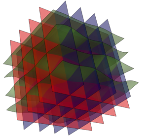
The resultant isopotential surfaces and streamsurfaces are shown in figure 5(b), forming a 3-D orthogonal grid which is distorted due to the heterogeneous conductivity field (3.1). This orthogonal grid of isosurfaces would be perfectly rectangular in the case of a homogeneous conductivity field, and would become more distorted with increasing conductivity variance, but the planar topology and orthogonal geometry would persist so long as the conductivity field can be represented as a scalar field. These streamsurfaces clearly illustrate the topologically planar structure of the flow field, such that the streamsurfaces (and indeed isopotential surfaces) foliate the flow domain in a lamellar fashion without knots or stagnation points. Streamlines of the flow then arise as the intersection of the  $\psi _1$ (red) and
  $\psi _2$ (blue) streamsurfaces, and so these arise topologically as straight lines in the flow (as opposed to closed or knotted orbits). Hence, the streamlines and kinematics of 3-D scalar Darcy flow is constrained by the topologically planar structure of these flows.

Figure 5. (a) Contour plot of the hydraulic conductivity field  $f=\ln k$ in the unit cube, (b) resultant level sets of the flow potential
  $\phi$ (grey) and streamfunctions
  $\psi _1$ (red) and
  $\psi _2$ (blue).
Conventional methods to solve Darcy flow and perform particle tracking typically use a FD or finite-volume method to solve the potential-based velocity field  $\boldsymbol {v}_\phi (\boldsymbol {x})$ at a finite set of points, which are then subject to piecewise-linear interpolation to generate a continuous representation of the velocity field. The algorithm of Pollock (Reference Pollock1988) is then typically used to advect particles by exploiting the piecewise linear nature of the velocity field, allowing solution of the particle position at cell faces via solution of algebraic equations rather than direct numerical solution of the advection ordinary differential equation (ODE) (2.7a,b). Whilst efficient, this approach introduces several sources of numerical errors that can allow numerically advected particles to ‘leak’ off their respective streamsurfaces, leading to spurious numerical artefacts unless care is taken. We briefly review these potential sources of error as follows and prescribe a simple solution to render particle tracking almost exact.
First, linear interpolation of the grid-based velocity data introduces serious errors in that the interpolated velocity field is no longer divergence free. Whilst such interpolation renders the local velocity field divergence free within each grid cell (as the velocity gradient is constant), there exist serious global divergence errors as the velocity gradient must be discontinuous at cell boundaries for all non-trivial flows. In addition, the mapping method inherent to the Pollock algorithm (Pollock Reference Pollock1988) introduces further errors as the higher-order gradients of the velocity field are ignored, allowing computed trajectories to deviate from their constraining streamlines. Such deviations then manifest as spurious numerical dispersion of particle trajectories, which can have serious ramifications for the study of e.g. solute dispersion in porous media. Whilst the divergence errors and velocity gradient discontinuities can be remedied by the use of explicitly divergence-free cubic interpolation schemes (Ravu et al. Reference Ravu, Rudman, Metcalfe, Lester and Khakhar2016), the issue of solving the advection ODE (2.7a,b) whilst enforcing particles to remain on streamfunctions persists. Although explicitly volume-preserving integration schemes (Wuispel Reference Wuispel1995) ensure particle trajectories are essentially volume preserving, and symplectic integration methods (Schlier & Seiter Reference Schlier and Seiter2000) ensure preservation of invariants in Hamiltonian systems (such as streamlines in 2-D flows), there is no known numerical method to enforce particles remain on streamsurfaces in steady 3-D flows. As such, the problem of spurious numerical dispersion persists even when the latest numerical methods (Robinson, Dash & Srinivasan Reference Robinson, Dash and Srinivasan2010; Suk Reference Suk2012; Craig, Ramadhan & Muffels Reference Craig, Ramadhan and Muffels2020) are applied to particle tracking under the potential-based velocity field  $\boldsymbol {v}_\phi (\boldsymbol {x})$. Such dispersion acts to break the topological kinematic constraints associated with scalar Darcy flow, hence care must be taken when interpreting results from such simulations.
These kinematic constraints can be enforced simply by using the streamfunction-based velocity field  $\boldsymbol {v}_\psi (\boldsymbol {x})$ as the streamfunctions are explicitly resolved and the streamlines are defined by the intersection of the streamfunctions
  $\psi _1$,
  $\psi _2$. In § 4 we develop a semi-orthogonal streamfunction coordinate system that allows the advection ODE (2.7a,b) to be expressed as the 1-D integral (2.8) along a streamline, explicitly eliminating the possibility of numerical dispersion off streamlines. Whilst numerical solution of (2.8) may still introduce numerical errors in the propagation distance along streamlines, these errors do not alter the Lagrangian kinematics of the flow. Similarly, numerical solution of the streamfunction equations (2.22), (2.23) may also introduce distortions in the streamsurfaces and streamlines of the flow, so long as the no stagnation condition (2.10a,b) is met, these distortions still adhere to the topological kinematic constraints of scalar Darcy flow.
A failure to explicitly impose these constraints becomes important in the prediction of transverse macrodispersion as such failure results in wandering of particle trajectories off streamlines, leading to spurious transverse dispersion. This becomes especially important when studying transverse macrodispersion in the case of zero local dispersion (i.e. to ascertain the contribution of macroscopic heterogeneity to transverse dispersion) as we show in § 5 that these kinematic constraints lead to zero macrodispersion in this case. Failure to enforce these constraints in the case means the only contribution to the measured transverse macrodispersion is numerical error.
4. Curvilinear streamline coordinates
As the magnitude of the Darcy velocity  $|\boldsymbol {v}|$ (and the pressure gradient
  $|\boldsymbol {\nabla }\phi |$) must be positive and finite, then from (2.9) the magnitude of the streamfunction gradients
  $|\boldsymbol {\nabla }\psi _1|$,
  $|\boldsymbol {\nabla }\psi _2|$ must also be everywhere positive and finite, as reflected by (2.10a,b). This condition means that any point
  $\boldsymbol {x}_0$ in scalar Darcy flow is uniquely defined by the local values of the fluid pressure and streamfunctions as
  $(\phi (\boldsymbol {x}_0),\psi _1(\boldsymbol {x}_0),\psi _2(\boldsymbol {x}_0))$. From (2.15a–c), this set of scalar functions represents a semi-orthogonal (in that some components are orthogonal but the streamfunctions are not mutually orthogonal) curvilinear streamline coordinate system
 \begin{equation} (\xi^1,\xi^2,\xi^3)\equiv(\phi,\psi_1,\psi_2),\quad \boldsymbol{\nabla}\xi^1\boldsymbol{\cdot} \boldsymbol{\nabla}\xi^2=\boldsymbol{\nabla}\xi^1 \boldsymbol{\cdot}\boldsymbol{\nabla}\xi^3=0,\end{equation}
which is invertible as the Jacobian  $J\equiv \det [\partial \xi ^i/\partial x_j]$ is everywhere non-zero. This coordinate system forms a convenient basis for studying the kinematics of scalar Darcy flow as it naturally encodes the kinematic constraints these flows as shall be shown in the following sections. The mapping from Cartesian coordinates
  $\boldsymbol {x}_0=x^1\boldsymbol {e}_1+x^2\boldsymbol {e}_2+x^3\boldsymbol {e}_3$ (where
  $x^j$,
  $\boldsymbol {e}_j$ respectively are the Cartesian coordinates and associated orthonormal basis vectors) to streamline coordinates
 \begin{equation} \boldsymbol{x}_0=\xi^1\boldsymbol{g}_1+\xi^2\boldsymbol{g}_2+\xi^3\boldsymbol{g}_3,\end{equation}
defines the covariant basis vectors  $\boldsymbol {g}_i$ of the curvilinear coordinate system (Aris Reference Aris1956) as
 \begin{equation} \boldsymbol{g}_i=\frac{\partial x^j}{\partial\xi^i}\boldsymbol{e}_j,\quad j=1,2,3,\end{equation}
where the Einstein summation convention is employed such that, unless indicated otherwise, summation is applied to repeat indices. From (4.3), the covariant metric coefficients are then given by  $g_{ij}=\boldsymbol {g}_i\cdot \boldsymbol {g}_j=g_{ji}$. The position vector
  $\boldsymbol {x}_0$ may also be expressed in terms of the contravariant basis vectors
  $\boldsymbol {g}^i$ as
 \begin{equation} \boldsymbol{x}_0=\xi_1\boldsymbol{g}^1+\xi_2\boldsymbol{g}^2+\xi_3\boldsymbol{g}^3,\end{equation}
where  $\xi _i$ are the contravariant components of
  $\boldsymbol {x}_0$, and
  $\boldsymbol {g}^i$ satisfy
 \begin{equation} \boldsymbol{g}^i=\frac{\partial\xi_i}{\partial x^j}\boldsymbol{e}_j,\quad j=1,2,3,\end{equation}
with contravariant metric coefficients  $g^{ij}=\boldsymbol {g}^i\cdot \boldsymbol {g}^j=g^{ji}$. The covariant and contravariant vectors are mutually orthogonal as
  $\boldsymbol {g}_i\cdot \boldsymbol {g}^j=\delta ^j_i$, where
  $\delta ^j_i$ is the Kronecker delta. Thus the contravariant and covariant basis vectors are respectively
 \begin{equation} \boldsymbol{g}^1=\boldsymbol{\nabla}\phi,\quad \boldsymbol{g}^2=\boldsymbol{\nabla}\psi_1,\quad \boldsymbol{g}^3=\boldsymbol{\nabla}\psi_2,\end{equation}
and
 \begin{equation} \left.\begin{aligned} \boldsymbol{g}_1&=\frac{\boldsymbol{\nabla}\phi}{|\boldsymbol{\nabla}\phi|^2},\quad \boldsymbol{g}_2=\boldsymbol{\nabla}\psi_1\frac{|\boldsymbol{\nabla}\psi_2|^2}{v^2}-\boldsymbol{\nabla}\psi_2 \frac{\boldsymbol{\nabla}\psi_1\boldsymbol{\cdot}\boldsymbol{\nabla}\psi_2}{v^2},\\ \boldsymbol{g}_3&=\boldsymbol{\nabla}\psi_2\frac{|\boldsymbol{\nabla}\psi_1|^2}{v^2}-\boldsymbol{\nabla}\psi_1 \frac{\boldsymbol{\nabla}\psi_1\boldsymbol{\cdot}\boldsymbol{\nabla}\psi_2}{v^2}, \end{aligned}\right\} \end{equation}
where  $v\equiv |\boldsymbol {v}|=\sqrt {|\boldsymbol {\nabla }\psi _1|^2| \boldsymbol {\nabla }\psi _2|^2-(\boldsymbol {\nabla }\psi _1\boldsymbol {\cdot }\boldsymbol {\nabla }\psi _2)^2}$. As shown in figure 6, orthogonality of the streamfunctions with respect to the flow potential renders the fluid velocity,
  $\boldsymbol {v}$ and basis vectors
  $\boldsymbol {g}_1$,
  $\boldsymbol {g}^1$ collinear, whilst the remaining covariant and contravariant basis vectors, along with the vorticity are all coplanar and perpendicular to these bases.

Figure 6. Streamline (blue), vorticity vector (red), covariant  $\boldsymbol {g}_i$ and contravariant
  $\boldsymbol {g}^i$ basis vectors of the streamline coordinate system. As indicated by the black ellipse, the contravariant and covariant vectors
  $\boldsymbol {g}_2$,
  $\boldsymbol {g}_3$,
  $\boldsymbol {g}^2$,
  $\boldsymbol {g}^3$ and vorticity
  $\boldsymbol \omega$ are all coplanar and perpendicular to the collinear velocity
  $\boldsymbol {v}$,
  $\boldsymbol {g}_1$ and
  $\boldsymbol {g}^1$ vectors.
From (4.5), the components of the contravariant metric tensor  $\boldsymbol {M}^{-1}$ may be written in terms of the potential and streamfunction gradients as
 \begin{equation} \boldsymbol{M}^{{-}1}\equiv\left[\begin{array}{ccc} g^{11} & 0 & 0 \\ 0 & g^{22} & g^{23} \\ 0 & g^{23} & g^{33}\ \end{array}\right]=\left[\begin{array}{ccc} |\boldsymbol{\nabla}\phi|^2 & 0 & 0 \\ 0 & |\boldsymbol{\nabla}\psi_1|^2 & \boldsymbol{\nabla}\psi_1\boldsymbol{\cdot}\boldsymbol{\nabla}\psi_2 \\ 0 & \boldsymbol{\nabla}\psi_1\boldsymbol{\cdot}\boldsymbol{\nabla}\psi_2 & |\boldsymbol{\nabla}\psi_2|^2\ \end{array}\right], \end{equation}
and so the covariant metric tensor  $\boldsymbol {M}$ is given by the inverse of (4.8) as
 \begin{equation} \boldsymbol{M}\equiv\left[\begin{array}{ccc} g_{11} & 0 & 0 \\ 0 & g_{22} & g_{23} \\ 0 & g_{23} & g_{33}\ \end{array}\right]=\frac{1}{v^2}\left[\begin{array}{ccc} \dfrac{v^2}{|\boldsymbol{\nabla}\phi|^2} & 0 & 0 \\ 0 & |\boldsymbol{\nabla}\psi_2|^2 & -\boldsymbol{\nabla}\psi_1\boldsymbol{\cdot}\boldsymbol{\nabla}\psi_2 \\ 0 & -\boldsymbol{\nabla}\psi_1\boldsymbol{\cdot}\boldsymbol{\nabla}\psi_2 & |\boldsymbol{\nabla}\psi_1|^2 \end{array}\right], \end{equation}
and the Jacobian  $J$ and metric scalar
  $g$ of the coordinate transform are then
 \begin{equation} J=\sqrt{g}\equiv\sqrt{\det[\boldsymbol{M}]}=\frac{1}{v|\boldsymbol{\nabla}\phi|}. \end{equation}
The above relationships can then be used to derive expressions for components of the velocity gradient  $\boldsymbol \epsilon \equiv \boldsymbol {\nabla }\boldsymbol {v}$ in the streamline coordinate system, where
  $\boldsymbol \epsilon =\epsilon ^i_j\boldsymbol {g}_i\otimes \boldsymbol {g}^j$, and
  $\sum _{i}\epsilon ^i_j=\boldsymbol {\nabla }\boldsymbol {\cdot }\boldsymbol {v}=0$. In Appendix B we show that the diagonal components of
  $\boldsymbol {\nabla }\boldsymbol {v}$ are given as
 \begin{equation} \epsilon^1_1=\frac{\partial v}{\partial s},\quad \epsilon^2_2={-}\frac{1}{2}\frac{\partial v}{\partial s}-m,\quad \epsilon^3_3={-}\frac{1}{2}\frac{\partial v}{\partial s}+m,\quad m\equiv\frac{v l^2}{2}\frac{\partial}{\partial s}\ln \frac{|\boldsymbol{\nabla}\psi_1|}{|\boldsymbol{\nabla}\psi_2|},\end{equation}
where  $l\equiv |\boldsymbol {\nabla }\psi _1|\,|\boldsymbol {\nabla }\psi _2|/v\geqslant 1$, and
  $s$ is the distance along a streamline. In streamline coordinates these components represent the principal strains experienced by a fluid element as it travels along a streamline, ignoring deformations arising from fluid shear contributions. The component
  $\epsilon ^1_1$ indicates that a fluid line element oriented along a streamline increases its length in proportion to the local velocity magnitude
  $v$ along a streamline. Conversely, the transverse components
  $\epsilon ^2_2$,
  $\epsilon ^3_3$ indicate that the length of fluid elements oriented transverse to the local velocity coordinate fluctuates due to contributions from the velocity fluctuations and changes in the streamfunction gradients as characterised by
  $m$. Appendix B also shows that the velocity gradient tensor in streamline coordinates is upper triangular
 \begin{equation} \boldsymbol\epsilon=\left(\begin{array}{ccc} \epsilon_{11} & \epsilon_{12} & \epsilon_{13}\\ 0 & \epsilon_{12} & 0\\ 0 & 0 & \epsilon_{33} \end{array}\right),\end{equation}
and the component  $\epsilon _{23}=0$ as a direct result of the helicity-free condition (2.4) as
 \begin{equation} h\equiv\boldsymbol{v}\boldsymbol{\cdot}(\boldsymbol{\nabla}\times\boldsymbol{v})=\boldsymbol{v} \cdot(:\boldsymbol{v})=\boldsymbol{v}_i\varepsilon_{ijk}\epsilon_{jk}=0,\end{equation}
where  $\varepsilon _{ijk}$ is the Levi-Civita tensor. As
  $\boldsymbol {v}=-k/\theta \boldsymbol {g}^1$, then (4.13) yields
  $\epsilon _{23}-\epsilon _{32}=0$, and since
  $\epsilon _{32}=0$, then
  $\epsilon _{23}=0$ also. In streamline coordinates
  $\epsilon _{23}$ represents the fluid shear (or vorticity) transverse to the local flow direction, hence,
  $\epsilon _{23}=0$ corresponds directly to the helicity-free condition. As shown in (Lester et al. Reference Lester, Dentz, Le Borgne and Barros2018), the component
  $\epsilon _{23}$ plays a critical role in coupling fluid deformation between the
  $1,2$- and
  $1,3$-planes in steady 3-D flows, leading to chaotic advection and exponential stretching of fluid elements. Conversely, the helicity-free condition
  $\epsilon _{23}=0$ in streamline coordinates effectively decouples the velocity gradient into two superposed shear flows as
 \begin{equation} \boldsymbol\epsilon=\boldsymbol\epsilon_{(12)}+\boldsymbol\epsilon_{(13)}= \left(\begin{array}{ccc} \dfrac{\epsilon_{11}}{2} & 0 & \epsilon_{13}\\ 0 & \epsilon_{12} & 0\\ 0 & 0 & 0 \end{array}\right)+\left(\begin{array}{ccc} \dfrac{\epsilon_{11}}{2} & 0 & \epsilon_{13}\\ 0 & 0 & 0\\ 0 & 0 & \epsilon_{33} \end{array}\right),\end{equation}
where  $\langle \epsilon _{11}\rangle =\langle \epsilon _{22}\rangle =\langle \epsilon _{33}\rangle =0$ and
  $\epsilon _i^i$ for
  $i=1:3$ are given by (4.11a–d). As the velocity gradient tensor governs the evolution of fluid deformation material line elements in the
  $1,2$- and
  $1,3$-planes are stretched via shear deformation in a similar fashion to that of steady 2-D flow. Whilst the coupling of intermittency, velocity fluctuations and shear deformation can lead to nonlinear growth of line elements in such flows (Dentz et al. Reference Dentz, Lester, Le Borgne and de Barros2016), such growth is algebraic and range from sublinear to ballistic behaviour. Hence, fluid deformation in steady 3-D scalar Darcy flow is analogous to that of steady 2-D flow in that the helicity-free condition constrains fluid elements to deform in a similar manner as two superposed 2-D shear flows.
5. Darcy flow kinematics of random porous media
5.1. Stationarity of streamfunctions
In § 4 we showed that the helicity-free condition constrains material elements to grow algebraically in time in a similar manner to that of 2-D steady flows (Dentz et al. Reference Dentz, Lester, Le Borgne and de Barros2016), rather than exponentially, as is the case for chaotic flows (Wiggins & Ottino Reference Wiggins and Ottino2004). In this section we derive the result that the helicity-free condition renders transverse hydrodynamic dispersion zero for porous media with a random hydraulic conductivity field that is smooth, finite and statistically stationary. We consider 3-D steady scalar Darcy flow in a porous medium with a heterogeneous conductivity field  $k(\boldsymbol {x})$ that is a random scalar function of space
  $\boldsymbol {x}=\{x_1,x_2,x_3\}$ that is statistically stationary in the mean flow direction
  $x_1$. We conceptualise the random conductivity field
  $k(\boldsymbol {x})$ to be a single realisation of a ensemble of fields that is described by a statistical conductivity model with prescribed correlation and heterogeneity structure, and consider transverse macrodispersion of a solute over the ensemble of realisations of
  $k(\boldsymbol {x})$. It is important to note, however, that we place no restrictions upon this statistical conductivity model beyond those of smoothness and finiteness of
  $k(\boldsymbol {x})$.
To remove boundary effects, we consider steady Darcy flow in an infinite 3-D domain  $\mathcal {D}:\boldsymbol {x}=(x_1,x_2,x_3)\in \mathbb {R}^3$ that is driven by a constant mean potential
  $\bar \phi =-G x_1$ with
  $G>0$ constant. The potential
  $\phi$ may then be decomposed into mean field
  $\bar \phi$ and fluctuating
  $\tilde \phi$ components as
 \begin{equation} \phi(\boldsymbol{x})=\bar\phi(\boldsymbol{x})+\tilde\phi(\boldsymbol{x}),\end{equation}
where the overbar denotes the spatial average
 \begin{equation} \bar{a}(\boldsymbol{x})\equiv\lim_{L\rightarrow\infty} \frac{1}{L^3}\int_{{-}L/2}^{L/2}\int_{{-}L/2}^{L/2} \int_{{-}L/2}^{L/2}a(\boldsymbol{x})\,\textrm{d} x_1\,\textrm{d} x_2\,\textrm{d} x_3,\end{equation}
and the tilde the remaining fluctuation  $\tilde {a}\equiv a-\bar {a}$, hence
  $\widetilde {\bar {a}}=0$. We make the assumption that as the conductivity field
  $k(\boldsymbol {x})$ is random and statistically stationary in the mean flow direction, then the corresponding velocity is also random and statistically stationary in this direction and so may be represented as
 \begin{equation} \boldsymbol{v}(\boldsymbol{x})=\bar{v}\hat{\boldsymbol{e}}_1+ \tilde{\boldsymbol{v}}(\boldsymbol{x}),\end{equation}
where  $\bar {v}$ is the constant mean velocity in the direction of the mean potential gradient and
  $\tilde {\boldsymbol {v}}(\boldsymbol {x})$ is a statistically stationary fluctuating component of the flux, where
  $\overline {\tilde {\boldsymbol {v}}}=\boldsymbol {0}$. The most general representation of the streamfunctions that correspond to this flow is then
 \begin{gather} \psi_1(\boldsymbol{x})=\bar\psi_1(\boldsymbol{x})+ \tilde\psi_1(\boldsymbol{x})=\alpha_{1,2}x_2+\alpha_{1,3}x_3+\tilde\psi_1(\boldsymbol{x}), \end{gather}
 \begin{gather}\psi_2(\boldsymbol{x})=\bar\psi_2(\boldsymbol{x})+ \tilde\psi_2(\boldsymbol{x})=\alpha_{2,2}x_2+\alpha_{2,3}x_3+\tilde\psi_2(\boldsymbol{x}), \end{gather}
where  $\alpha _{i,j}$ are arbitrary constants and
  $\tilde \psi _1(\boldsymbol {x})$,
  $\tilde \psi _2(\boldsymbol {x})$ are random fluctuations that satisfy
  $\overline {\tilde \psi }_1=0$,
  $\overline {\tilde \psi }_2=0$. The stagnation-free flow condition (2.10a,b) then corresponds to the condition
 \begin{equation} \boldsymbol{\nabla}\tilde\psi_i(\boldsymbol{x})\boldsymbol{\cdot} \boldsymbol{\nabla}\bar\psi_i< C_i^2\equiv\|\boldsymbol{\nabla}\bar\psi_i\|^2,\quad i=1:2,\enspace \forall\boldsymbol{x}\in\mathcal{D} \end{equation}
for the fluctuations  $\tilde \psi _i(\boldsymbol {x})$ where
  $C_i$ is a constant that characterises the magnitude of the constant gradient
  $\boldsymbol {\nabla }\bar \psi _i$. Inserting (5.4), (5.5) into (2.9) then yields
 \begin{align} \boldsymbol{v}(\boldsymbol{x})&=(\alpha_{1,2}\alpha_{2,3}-\alpha_{1,3}\alpha_{2,2}) \hat{\boldsymbol{e}}_1+\boldsymbol{\nabla}\tilde{\psi}_1\times\boldsymbol{\nabla}\tilde{\psi}_2 \nonumber\\ &\quad +\alpha_{1,2}\boldsymbol{\nabla}\times(\tilde\psi_1\hat{\boldsymbol{e}}_2)-\alpha_{2,2} \boldsymbol{\nabla}\times(\tilde\psi_2\hat{\boldsymbol{e}}_2)+\alpha_{1,3}\boldsymbol{\nabla} \times(\tilde\psi_1\hat{\boldsymbol{e}}_3)-\alpha_{2,3}\boldsymbol{\nabla} \times(\tilde\psi_2\hat{\boldsymbol{e}}_3). \end{align}
From Stokes’ theorem, the spatial average of the terms  $\boldsymbol {\nabla }\times (\tilde \psi _i\hat {\boldsymbol {e}}_j)$ for
  $i=1:2$,
  $j=2:3$ in (5.7) may be expressed as
 \begin{equation} \overline{\boldsymbol{\nabla}\times(\tilde\psi_i\hat{\boldsymbol{e}}_j)}=\lim_{L\rightarrow\infty} \frac{1}{L^3}\int_{V_{L^3}}\boldsymbol{\nabla}\times(\tilde\psi_i\hat{\boldsymbol{e}}_j)\,\textrm{d}\boldsymbol{x}^3= \lim_{L\rightarrow\infty}\frac{1}{L^3}\oint_{S_{L^3}}\tilde\psi_i \hat{\boldsymbol{e}}_j\,\textrm{d}\boldsymbol{x}^2=\boldsymbol{0}, \end{equation}
where  $V_{L^3}$ denotes the volume of a cube of length
  $L$ centred at
  $\boldsymbol {x}=0$ and
  $S_{L^3}$ denotes its surface. As
  $\tilde \psi _i$ is finite the surface integral above scales as
  $L^2$, and so
  $\overline {\boldsymbol {\nabla }\times (\tilde \psi _i\hat {\boldsymbol {e}}_j)}=\boldsymbol {0}$ in the limit
  $L\rightarrow \infty$. Via similar reasoning and using (2.11), the spatial average of
  $\boldsymbol {\nabla }\tilde {\psi }_1\times \boldsymbol {\nabla }\tilde {\psi }_2= \boldsymbol {\nabla }\times (\tilde \psi _1\boldsymbol {\nabla }\tilde \psi _2)$ in (5.7) is also zero
 \begin{equation} \overline{\boldsymbol{\nabla}\tilde{\psi}_1\times \boldsymbol{\nabla}\tilde{\psi}_2}= \lim_{L\rightarrow\infty}\frac{1}{L^3}\int_{V_{L^3}} \boldsymbol{\nabla}\times(\tilde\psi_1\boldsymbol{\nabla}\tilde\psi_2)\,\textrm{d}\boldsymbol{x}^3= \lim_{L\rightarrow\infty}\frac{1}{L^3}\oint_{S_{L^3}}\tilde\psi_1\boldsymbol{\nabla} \tilde\psi_2 \,\textrm{d}\boldsymbol{x}^2=\boldsymbol{0}. \end{equation}
Hence, the mean of (5.7) is
 \begin{equation} \bar{v}=\alpha_{1,2}\alpha_{2,3}-\alpha_{1,3}\alpha_{2,2}, \end{equation}
and so the fluctuating component is then given by
 \begin{align} \tilde{\boldsymbol{v}}(\boldsymbol{x}) &= \boldsymbol{\nabla}\tilde{\psi}_1\times\boldsymbol{\nabla}\tilde{\psi}_2+ \alpha_{1,2}\boldsymbol{\nabla}\times(\tilde{\psi}_1\hat{\boldsymbol{e}}_2)-\alpha_{2,2}\boldsymbol{\nabla} \times(\tilde{\psi}_2\hat{\boldsymbol{e}}_2) \nonumber\\ &\quad +\alpha_{1,3}\boldsymbol{\nabla}\times(\tilde{\psi}_1\hat{\boldsymbol{e}}_3)-\alpha_{2,3} \boldsymbol{\nabla}\times(\tilde{\psi}_2\hat{\boldsymbol{e}}_3). \end{align}
As  $\tilde {\boldsymbol {v}}$ is statistically stationary in the mean flow direction, the individual terms in (5.11) are also statistically stationary in this direction, hence, the fluctuations
  $\tilde \psi _i(\boldsymbol {x})$ must also be statistically stationary in this direction. As the level sets of the mean streamfunctions
  $\bar \psi _i$ correspond to the planes defined by the equations
 \begin{equation} \bar\psi_i(x_2,x_3)=\alpha_{i,2}x_2+\alpha_{i,3}x_3,\quad i=1:2,\end{equation}
then the level sets of the total streamfunctions  $\psi _i(\boldsymbol {x})$ fluctuate about these planes in a statistically stationary manner as per figure 7. As shown in figure 7, we define
  $\delta \ell _i(\boldsymbol {x}_0)$ as the distance from the point
  $\boldsymbol {x}_0$ with streamfunction
  $\psi _{i,0}\equiv \psi _i(\boldsymbol {x}_0)$ and a point
  $\boldsymbol {x}_0^\prime$ on the corresponding plane
  $\bar \psi _i(\boldsymbol {x})=\psi _{i,0}$ (given by (5.12)), where the straight line from
  $\boldsymbol {x}_0$ and
  $\boldsymbol {x}_0^\prime$ is collinear with
  $\boldsymbol {\nabla }\bar{\psi}_i$, i.e. it is normal to the level sets of
  $\bar \psi _i$. Thus the vector
  $\boldsymbol {x}_0-\boldsymbol {x}_0^\prime$ may be expressed as
 \begin{equation} \boldsymbol{x}_0-\boldsymbol{x}_0^\prime=a\boldsymbol{\nabla}\bar\psi_i, \end{equation}
where  $a$ is an arbitrary scalar. By rearranging, we find that
 \begin{equation} a=\frac{\delta\ell_i(\boldsymbol{x}_0)}{C_i}= \frac{(\boldsymbol{x}_0-\boldsymbol{x}_0^\prime)\boldsymbol{\cdot} \boldsymbol{\nabla}\bar\psi_i}{\boldsymbol{\nabla}\bar\psi_i \boldsymbol{\cdot}\boldsymbol{\nabla}\bar\psi_i},\quad i=1,2, \end{equation}
and as
 \begin{equation} \psi_{i,0}\equiv\psi_i(\boldsymbol{x}_0)=\bar\psi_i(\boldsymbol{x}_0)+ \tilde\psi_i(\boldsymbol{x}_0)=\bar\psi_i(\boldsymbol{x}_0^\prime), \end{equation}
then
 \begin{equation} \tilde\psi_i(\boldsymbol{x}_0)=\bar\psi_i(\boldsymbol{x}_0^\prime)- \bar\psi_i(\boldsymbol{x}_0)=(\boldsymbol{x}_0-\boldsymbol{x}_0^\prime) \boldsymbol{\cdot}\boldsymbol{\nabla}\bar\psi_i. \end{equation}
Hence, the spacing  $\delta \ell _i(\boldsymbol {x})$ between the level set of the streamfunction
  $\psi _i(\boldsymbol {x})$ and the planar level set of its mean component
  $\bar \psi _i(\boldsymbol {x})$ is just the rescaled fluctuation
 \begin{equation} \delta\ell_i(\boldsymbol{x}_0)=\frac{\tilde\psi_i(\boldsymbol{x}_0)}{C_i},\quad i=1,2.\end{equation}
As  $\tilde \psi _i(\boldsymbol {x})$ is statistically stationary,
  $\delta \ell _i(\boldsymbol {x})$ is also a statistically stationary random variable with zero mean, and so the streamsurfaces given by the level sets of
  $\psi _i$ fluctuate about the planar surfaces corresponding to the level sets of
  $\bar \psi _i$.

Figure 7. Schematic of  $\psi _1$ (red, solid) and
  $\psi _2$ (blue, solid) streamsurfaces (solid) and
  $\bar \psi _1$ (red, dashed) and
  $\bar \psi _2$ (blue, dashed) level sets in a plane of constant
  $x_1$, depicting points
  $\boldsymbol {x}_0$,
  $\boldsymbol {x}_0^\prime$ and length
  $\delta \ell _i(\boldsymbol {x}_0)$ as described in the text.
5.2. Spacing between streamfunctions
We may also derive an expression for the transverse distance (i.e. transverse to the mean flow direction  $\hat {\boldsymbol {e}}_1$) between two arbitrary streamlines
  $a$ and
  $b$ (shown in figure 8) denoted respectively by the streamfunction pairs
  $(\psi _{1,a},\psi _{2,a})$,
  $(\psi _{1,b},\psi _{2,b})$. We denote the positions of the
  $a-$ and
  $b-$streamlines in the
  $(x_2,x_3)$ plane (at an arbitrary value of
  $x_1=X_1$) as
  $\boldsymbol {x}_a$ and
  $\boldsymbol {x}_b$, respectively, such that
 \begin{equation} \psi_i(X_1,\boldsymbol{x}_a)=\psi_{i,a},\quad\psi_i(X_1,\boldsymbol{x}_b)=\psi_{i,b},\quad i=1,2. \end{equation}
We also denote the positions of the intersections of the level sets of  $\bar \psi _1(\boldsymbol {x})$ and
  $\bar \psi _2(\boldsymbol {x})$ that correspond to
  $\psi _1$,
  $\psi _2$ respectively as
  $\boldsymbol {x}_a^\prime$ and
  $\boldsymbol {x}_b^\prime$, such that
 \begin{equation} \psi_i(X_1,\boldsymbol{x}_a)=\bar\psi_i(\boldsymbol{x}_a^\prime),\quad \psi_i(\boldsymbol{x}_b)=\bar\psi_i(X_1,\boldsymbol{x}_b^\prime),\quad i=1,2. \end{equation}
Figure 8. Schematic of spacing  $\ell _{ab}$ between streamlines located at
  $\boldsymbol {x}_a$ and
  $\boldsymbol {x}_b$ (with corresponding streamfunction pairs
  $(\psi _{1,a},\psi _{1,b})$,
  $(\psi _{2,a},\psi _{2,b})$) in a cross-sectional plane of constant
  $x_1$. The points
  $\boldsymbol {x}_a^\prime$ and
  $\boldsymbol {x}_b^\prime$ denote the intersection of the level sets of
  $(\bar \psi _{1,a},\bar \psi _{1,b})$,
  $(\bar \psi _{2,a},\bar \psi _{2,b})$), respectively, and
  $\bar {\ell }_{ab}$ is the spacing between these points.
Solving these equations for  $\boldsymbol {x}_a^\prime$,
  $\boldsymbol {x}_b^\prime$ then yields
 \begin{gather} \boldsymbol{x}_a^\prime=\frac{1}{\bar{v}}\left(0,\alpha_{2,3}\psi_{1,a}-\alpha_{1,3} \psi_{2,a},\alpha_{1,2}\psi_{2,a}-\alpha_{2,2}\psi_{1,a}\right), \end{gather}
 \begin{gather}\boldsymbol{x}_b^\prime=\frac{1}{\bar{v}}\left(0,\alpha_{2,3}\psi_{1,b}-\alpha_{1,3} \psi_{2,b},\alpha_{1,2}\psi_{2,b}-\alpha_{2,2}\psi_{1,b}\right). \end{gather}
From these coordinates, the coordinates of  $\boldsymbol {x}_a$,
  $\boldsymbol {x}_b$ are then
 \begin{gather} \boldsymbol{x}_a=\boldsymbol{x}_a^\prime+\delta\ell_1(\boldsymbol{x}_a)\boldsymbol{\nabla} \bar\psi_1+\delta\ell_2(\boldsymbol{x}_a)\boldsymbol{\nabla}\bar\psi_2, \end{gather}
 \begin{gather}\boldsymbol{x}_b=\boldsymbol{x}_b^\prime+\delta\ell_1(\boldsymbol{x}_b)\boldsymbol{\nabla} \bar\psi_1+\delta\ell_2(\boldsymbol{x}_b)\boldsymbol{\nabla}\bar\psi_2, \end{gather}
and so the points  $\boldsymbol {x}_a$,
  $\boldsymbol {x}_b$ essentially take a random walk around the fixed points
  $\boldsymbol {x}_a^\prime$,
  $\boldsymbol {x}_b^\prime$ as the
  $a-$,
$a-$,  $b-$streamlines propagate in the
  $1$-direction. Thus the distance
  $\bar \ell _{ab}(X_1)$ between the points
  $\boldsymbol {x}_a^\prime$ and
  $\boldsymbol {x}_b^\prime$ in the
  $x_1=X_1$ plane is given by the norm
 \begin{equation} \bar\ell_{ab}(X_1)=\|\boldsymbol{x}_a^\prime-\boldsymbol{x}_b^\prime\|= \frac{1}{v}\sqrt{ \left(\alpha_{1,3}\varDelta\psi_2-\alpha_{2,3}\varDelta\psi_1\right)^2+ \left(\alpha_{2,2}\varDelta\psi_1-\alpha_{2,3}\varDelta\psi_2\right)^2 }, \end{equation}
where  $\varDelta \psi _i\equiv \psi _{2,a}-\psi _{2,b}$ for
  $i=1,2$. The distance
  $\bar \ell _{ab}$ between the points
  $\boldsymbol {x}_a$ and
  $\boldsymbol {x}_b$ is then
 \begin{equation} \ell_{ab}(X_1)=\|\boldsymbol{x}_a-\boldsymbol{x}_b\|=\bar\ell_{ab}(X_1)+\tilde\ell_{ab}(X_1), \end{equation}
where  $\tilde \ell _{ab}(X_1)=F(\tilde \psi _1(\boldsymbol {x}),\tilde \psi _2(\boldsymbol {x}))$ is the fluctuation in the transverse distance between the
  $a-$ and
  $b-$streamlines as they propagate in the
  $1-$direction through the medium. As
  $\tilde \ell _{ab}(X_1)$ only depends upon the streamline fluctuations
  $\tilde \psi _1(\boldsymbol {x})$,
  $\tilde \psi _2(\boldsymbol {x})$, then the spacing fluctuation
  $\tilde \ell _{ab}(X_1)$ is also statistically stationary in the
  $1-$direction. Thus, streamlines neither diverge nor converge as they propagate with the mean flow in the
  $1$-direction.
5.3. Transverse macrodispersion
We quantify the impact of this behaviour upon transverse macrodispersion by considering evolution of the steady scalar concentration field  $c(x_1,x_2,x_3)$ of a solute plume as it is advected through the flow field in the absence of local dispersion (such as molecular diffusion). We consider evolution of the concentration field of a solute plume under two scenarios. These two scenarios involve the injection of a solute plume into the flow field at the plane
  $x_1=0$ as a Gaussian line source that is centred along either the line
  $x_2=0$ or
  $x_3=0$ as per the inlet conditions
 \begin{equation} c(0,x_2,x_3)=c_{0,j}(x_j)=c_{0,max}\exp\left(-\frac{x_j^2}{2\sigma^2_{c,0}}\right),\quad j=2,3.\end{equation}
The asymptotic transverse macrodispersion coefficient  $D_{T,\infty ,j}$ in both the
  $j=2$ and
  $j=3$ directions is then defined as the ensemble average (over the ensemble of scalar conductivity fields) of the asymptotic growth rate of the transverse spatial variance (in the
  $x_j$ coordinate) of the concentration field
  $\sigma _{c,j}^2$ defined as
 \begin{equation} \sigma_{c,j}^2(x_1)\equiv\int_{-\infty}^\infty c(x_1,x_2,x_3)x_j^2 \,\textrm{d} x_j,\quad j=2,3,\end{equation}
where from (5.26),  $\sigma _{c,j}^2(0)=\sigma _{c,0}^2$. The asymptotic transverse macrodispersion coefficients are then
 \begin{equation} D_{T,\infty,j}=\lim_{x_1\rightarrow\infty}\left\langle \frac{\textrm{d}\sigma_{c,j}^2}{\textrm{d} x_1}\right\rangle,\quad j=2,3,\end{equation}
where the angled brackets denote the ensemble average which, due to ergodicity of the conductivity field and  $x_{1-j}$-independent nature of the inlet condition (5.26), may be expressed as
 \begin{equation} \left\langle\frac{\textrm{d}\sigma_{c,j}^2}{\textrm{d} x_1}\right\rangle= \lim_{L\rightarrow\infty}\int_{{-}L/2}^{L/2}\frac{\textrm{d}\sigma_{c,j}^2}{\textrm{d} x_1}\textrm{d} x_{1-j}.\end{equation}
In § 4, the transform between the Cartesian  $(x_1,x_2,x_3)$ and streamline
  $(\phi ,\psi _1,\psi _2)$ coordinate systems was shown to be unique, and so each Cartesian coordinate may be uniquely expressed as
 \begin{equation} x_i=x_i(\phi,\psi_1,\psi_2),\quad i=1:3.\end{equation}
As  $\partial \phi /\partial x_1<0\ \forall \boldsymbol {x}\in \mathcal {D}$, the coordinate
  $x_1$ may be uniquely defined as
  $x_1=x_1(\phi )$ along a single streamline. It shall prove useful to then define the Lagrangian coordinates
  $X_2$,
  $X_3$ such that
  $X_2(x_1;\psi _1,\psi _2)$,
  $X_3(x_1;\psi _1,\psi _2)$ respectively denote the
  $x_2$ and
  $x_3$ coordinates of a point at the
  $x_1$ coordinate on a streamline that was initially at coordinate
  $(0,x_2,x_3)$ at
  $x_1=0$, i.e.
 \begin{equation} X_2(0;\psi_1,\psi_2)\equiv x_2\quad X_3(0;\psi_1,\psi_2)\equiv x_3.\end{equation}
As the streamfunctions are invariant along a streamline, we shall henceforth express these coordinates as  $X_2(x_1)$,
  $X_3(x_1)$ with the understanding these coordinates refer to a unique streamline. Similar to the streamfunctions, we may then decompose these Lagrangian coordinates into mean field and fluctuating terms as
 \begin{equation} X_2(x_1)=\bar{X}_2+\tilde{X}_2(x_1),\quad X_3(x_1)=\bar{X}_3+\tilde{X}_3(x_1),\end{equation}
where  $\bar {X}_2$,
  $\bar {X}_3$ are invariant with
  $x_1$. From (5.17), the fluctuations
  $\tilde {X}_j$ may then be related to the streamfunction fluctuations as
 \begin{equation} \tilde{X}_j(x_1)=\sum_{i=1}^2\frac{\delta\ell_i(\boldsymbol{x})}{C_i}\boldsymbol{\nabla} \bar\psi_i\cdot\hat{\boldsymbol{e}}_j=\sum_{i=1}^2\frac{\alpha_{i,j}}{C_i^2} \tilde\psi_i(\boldsymbol{x}),\quad j=2,3.\end{equation}
Combining (5.31a,b)–(5.33), the Lagrangian coordinates  $X_j$ may then also be expressed in terms of the streamfunction fluctuations as
 \begin{equation} X_j(x_1)=x_j-\delta x_j(x_1)=x_j-\sum_{i=1}^2\frac{\alpha_{i,j}}{C_i^2} \left(\tilde\psi_i(0)-\tilde\psi(x_1)\right),\quad j=2,3,\end{equation}
where  $\delta x_j(x_1)\equiv \tilde {X}_j(0)-\tilde {X}_j(x_1)$ and
  $\tilde \psi _i(x_1)\equiv \tilde \psi _i(x_1,X_2(x_1),X_3(x_1))$. These results shall then be used to derive expressions for evolution of the transverse macrodispersion as follows.
In the absence of local dispersion, the solute concentration field  $c$ evolves according to the steady advection partial differential equation (PDE)
 \begin{equation} \boldsymbol{v}(\boldsymbol{x})\boldsymbol{\cdot}\boldsymbol{\nabla} c(\boldsymbol{x})=0,\quad c(\boldsymbol{x})|_{x_1=0}=c_0(x_2,x_3).\end{equation}
From this hyperbolic PDE, the scalar concentration  $c$ is constant along streamlines, hence, the concentration field at arbitrary distances in the longitudinal coordinate
  $x_1$ can be mapped back to the initial concentration field
  $c_0(x_2,x_3)$ via the Lagrangian coordinates
 \begin{equation} c(x_1,x_2,x_3)=c_0(X_2(x_1;\psi_1,\psi_2),X_3(x_1;\psi_1,\psi_2))=c_0(X_2(x_1),X_3(x_1)).\end{equation}
Inserting (5.34) and (5.36) into (5.27) then yields
 \begin{align} \sigma_{c,j}^2(x_1)&=\int_{-\infty}^\infty c_0(X_2,X_3)x_j^2 \,\textrm{d} x_j, \nonumber\\ &=\int_{-\infty}^\infty c_0(X_2,X_3)(X_j+\delta x_j)^2 \,\textrm{d} X_j, \nonumber\\ &=\sigma_c^2(0)+\int_{-\infty}^\infty c_0(X_2,X_3)(\delta x_j^2+2X_j\delta x_2) \,\textrm{d} X_j,\quad j=2,3. \end{align}
Using (5.29) to take the ensemble average of (5.37) then yields  $\langle \delta x_j\rangle =0$ and
 \begin{equation} \langle\sigma_{c,j}^2\rangle=\sigma_{c,0}^2+\langle\delta x_j^2\rangle=\sigma_{c,0}^2+ \frac{\alpha^2_{1,j}}{C_1^2}\langle\delta \psi_1^2\rangle+2\frac{\alpha_{1,j}\alpha_{2,j}}{C_1C_2} \langle\delta\psi_1\delta\psi_2\rangle+\frac{\alpha^2_{2,j}}{C_2^2}\langle\delta\psi_2^2\rangle,\quad j=2,3,\end{equation}
where
 \begin{equation} \delta\psi_i(x_1)\equiv\tilde\psi_i(0)-\tilde\psi_i(x_1),\quad i=1,2, \end{equation}
and the ensemble average  $\langle \delta x_j\rangle =0$. Thus auto- and cross-correlation of the streamline fluctuations lead to an increase of the transverse second central moment of the concentration plume. Due to the random nature of the conductivity field, the autocorrelation of streamline fluctuations must decay to zero along a streamline as
 \begin{equation} \lim_{x_1\rightarrow\infty}\langle\tilde\psi_i(x_1)\tilde\psi_i(0)\rangle=0, \end{equation}
and we may approximate the evolution of this autocorrelation as a first-order process
 \begin{equation} \langle\tilde\psi_i(x_1)\tilde\psi_i(0)\rangle\approx\sigma_{\psi_i}^2\exp({-}x_1/\zeta),\quad i=1,2,\end{equation}
where the variance  $\sigma _{\tilde \psi _i}^2=\langle \tilde \psi _i(x_1)^2\rangle$ is constant and the parameter
  $\zeta$ characterises the decay of the autocorrelation. Without loss of generality we assume that the streamfunction fluctuations are partially correlated as
  $\langle \tilde \psi _1\tilde \psi _2\rangle =\beta \langle \tilde \psi _1^2\rangle$ where
  $\beta \equiv \sigma _{\psi _1}^2/\sigma _{\psi _1\psi _2}^2$ is a constant. Combining these results, we find
 \begin{equation} \langle\delta\psi_i^2\rangle\approx2\sigma_{\psi_i}^2(1-\exp({-}x_1/\zeta)),\quad \langle\delta\psi_1\delta\psi_2\rangle\approx2\sigma_{\psi_{12}}^2(1-\exp({-}x_1/\zeta)),\end{equation}
and so the transverse spatial variance of the solute plume evolves approximately as
 \begin{equation} \langle\sigma_{c,j}^2\rangle\approx\sigma_{c,0}^2+\sigma_{\psi}^2 \left(1-\exp({-}x_1/\zeta)\right),\quad j=2,3,\end{equation}
where
 \begin{equation} \sigma_{j,\psi}^2\equiv2\sigma_{\psi_1}^2\frac{\alpha^2_{1,j}}{C_1^2}+4\sigma_{\psi_1\psi_2}^2 \frac{\alpha_{1,j}\alpha_{2,j}}{C_1C_2}+2\sigma_{\psi_2}^2\frac{\alpha^2_{2,j}}{C_2^2},\quad j=2,3. \end{equation}
Hence, the streamfunctions act to increase transverse variance of the solute plume due to the decay of auto- and cross-correlations between the streamfunction fluctuations. As these correlations must decay to zero, in the asymptotic limit we recover the exact result that the transverse variance converges to a constant value
 \begin{equation} \lim_{x_1\rightarrow\infty}\langle\sigma_{c,j}^2\rangle=\sigma_{c,0}^2+\sigma_{j,\psi}^2,\quad j=2,3,\end{equation}
as the streamfunction fluctuations  $\tilde \psi _1$,
  $\tilde \psi _2$ are statistically stationary. Hence, asymptotic transverse macrodispersion is zero in the absence of local dispersion
 \begin{equation} D_{T,\infty,j}=\lim_{x_1\rightarrow\infty}\left\langle \frac{\textrm{d}\sigma_{c,j}^2(x_1)}{\textrm{d} x_1}\right\rangle=0,\quad j=2,3,\end{equation}
in scalar 3-D Darcy flow with a random, statistically stationary conductivity field.
This is in direct contrast to non-integrable steady 3-D flows, where material elements oriented transverse to the mean flow direction may continually grow without bound in the mean flow direction (at e.g. an exponential rate in the case of chaotic flows). Such growth is directly attributable to the absence of invariant streamfunctions for non-integrable 3-D flows, and so the streamlines of the flow can wander throughout the flow domain without being confined to coherent, topologically planar streamsurfaces.
It has been shown (Attinger et al. Reference Attinger, Dentz and Kinzelbach2004) that steady 2-D flows with topologically open streamlines also exhibit zero transverse hydrodynamic dispersion. For steady 2-D flow (whether Darcy flow or otherwise), the topological constraints associated with the foliation of streamlines within 2-D surface (such that streamlines cannot cross) combined with conservation of mass ensures that the transverse separation between neighbouring streamlines may only fluctuate about a mean value (Dentz et al. Reference Dentz, Lester, Le Borgne and de Barros2016). This constraint on streamline behaviour then leads to zero transverse hydrodynamic dispersion in steady 2-D Darcy flow. For the case of 3-D scalar Darcy flow, the existence of a pair of topologically planar streamfunctions  $\psi _1$,
  $\psi _2$ renders the kinematics of these flows very similar to that of steady 2-D Darcy flow. This behaviour is a direct result of the integrable and helicity-free nature of scalar Darcy flow.
From the result (5.46), a natural question is to ask what are the implications for transverse dispersion in the presence of local scale dispersion? As significant transverse hydrodynamic dispersion has been repeatedly observed in both numerical (Janković et al. Reference Janković, Fiori and Dagan2003, Reference Janković, Steward, Barnes and Dagan2009; Beaudoin, de Dreuzy & Erhel Reference Beaudoin, de Dreuzy and Erhel2010) and experimental (Adams & Gelhar Reference Adams and Gelhar1992) studies of macroscopic solute transport, in the absence of transverse hydrodynamic dispersion for purely advective transport, suggest one of two possible scenarios.
The first scenario is that transverse local scale dispersion may play an important role in triggering macroscopic transverse dispersion. This would imply that the limit of transverse local scale dispersion to zero is singular in the following sense. Let us denote the transient transverse dispersion coefficient by  $D_T(t,D_0)$, where
  $D_0$ is the local scale dispersion coefficient. Under this scenario, our results suggest that the limits of
  $t \to \infty$ and
  $D_0 \to 0$ do not commute. This means that
 \begin{equation} \lim_{D_0 \to 0} \lim_{t \to \infty} D_T(t,D_0) = D^\ast_{T,\infty} > 0, \end{equation}
while
 \begin{equation} \lim_{t \to \infty} \lim_{D_0 \to 0} D_T(t,D_0) = 0. \end{equation}
However, recent studies (de Moura Reference de Moura2014; Cerbelli et al. Reference Cerbelli, Giona, Gorodetskyi and Anderson2017) have shown that the advection–diffusion equation is only singular with respect to diffusion coefficient  $D_0$ when the advection field is everywhere chaotic, otherwise the advection–diffusion is non-singular in the limit
  $D_0\rightarrow 0$. As the helicity-free nature of steady, scalar Darcy flow renders it non-chaotic, it is possible that this first scenario may not hold. If this is the case, the second scenario is that scalar Darcy flow is not a realistic model for flow and transport in heterogeneous porous media. Under this scenario, the kinematic constraints associated with scalar Darcy flow preclude macroscopic transverse dispersion in the limit of vanishing local dispersion, i.e.
 \begin{equation} \lim_{D_0 \to 0} \lim_{t \to \infty} D_T(t,D_0) = 0. \end{equation}
An inability to predict macroscopic transverse dispersion in the limit of vanishing local dispersion would represent a significant failing of scalar Darcy flow and so it is important to determine which of the above scenarios is correct. This is the topic of ongoing research and is a question we aim to resolve in the near future.
This result is in contradiction with previous numerical studies (Janković et al. Reference Janković, Steward, Barnes and Dagan2009; Beaudoin & de Dreuzy Reference Beaudoin and de Dreuzy2013) that have reported non-zero transverse macrodispersion in the purely advective case. A possible reason for this discrepancy is that these studies involve numerical methods that do not explicitly conform to the kinematic constraints associated with scalar Darcy flow, and so may involve spurious numerical dispersion. Beaudoin & de Dreuzy (Reference Beaudoin and de Dreuzy2013) observe that ‘in 3D, flow lines expand within a widening cone and their extension in the direction transverse to the main flow direction is not limited’, which is inconsistent with the kinematic constraint that streamlines in steady 3-D Darcy flow in a statistically stationary, scalar conductivity field cannot diverge without bound. Similarly, Janković et al. (Reference Janković, Steward, Barnes and Dagan2009) observe non-zero transverse dispersion in 3-D Darcy flow with impermeable inclusions. Since the conductivity  $k$ is discontinuous at the boundaries of these inclusions, the vorticity, and hence helicity, is undefined in these flows. As such, these flows may exhibit the kinematics of non-zero helicity flow. Janković et al. (Reference Janković, Steward, Barnes and Dagan2009) identify helical flow, described as ‘advective mixing’ and ‘complex intertwining of streamlines’, as the generator of non-zero transverse macrodispersion.
We also note that several workers have shown numerically (Chiogna et al. Reference Chiogna, Cirpka, Rolle and Bellin2015) and experimentally (Ye et al. Reference Ye, Chiogna, Cirpka, Grathwohl and Rolle2015) that Darcy flows in porous media with scalar conductivity fields that are statistically anisotropic appear to exhibit streamlines that do not conform to distinct topologically planar streamsurfaces but rather appear to twist and wander more freely throughout the flow domain. We note, however, that these conductivity fields are not smooth, and so the associated discontinuities in the velocity gradient field violate the smoothness assumptions (Arnol'd Reference Arnol'd1965) associated with the existence of distinct streamfunctions in the flow. More broadly, scalar Darcy flows in porous media with discontinuous conductivity fields may not conform to the kinematic constraints inherent to helicity- and stagnation-free flows.
These kinematic constraints also do not apply to porous media with tensorial hydraulic conductivity. Fluid flow in such media is described by the tensorial Darcy equation
 \begin{equation} \boldsymbol{v}={-}\boldsymbol{K}(\boldsymbol{x})\boldsymbol{\cdot}\boldsymbol{\nabla}\phi(\boldsymbol{x}),\end{equation}
where  $\boldsymbol {K}(\boldsymbol {x})$ is the tensorial hydraulic conductivity field. For (5.50), the helicity-free condition (2.4) no longer applies (so long as
  $\boldsymbol {K}(\boldsymbol {x})\neq k(\boldsymbol {x})\boldsymbol {I}$), hence, the flow is no longer integrable and the invariant streamfunctions
  $\psi _1$,
  $\psi _2$ do not exist for these flows.
6. Conclusions
We have considered the Lagrangian kinematics of 3-D scalar Darcy flow, which are characterised by their singularity- and helicity-free nature. We show that the integrable nature of these flows admits a pair of topologically planar invariant streamfunctions that are single valued throughout the flow domain. We derive governing equations for the streamfunction pair and use these streamfunctions to develop a semi-orthogonal streamline coordinate system for these flows. Using this coordinate system, we show that, for statistically stationary porous media, the transverse hydrodynamic dispersion for purely advective transport is zero. These results stem from the fact that the kinematics of scalar Darcy flow are overwhelmingly two-dimensional in character; here, streamlines are confined to topologically planar 2-D streamsurfaces and so the only persistent fluid deformation is in the longitudinal direction, where fluid elements grow algebraically in time. These kinematics significantly constrain dispersion and mixing in 3-D porous media and provide a basis for the derivation of 3-D stochastic transport and mixing models. While we have investigated the impact of these kinematic constraints upon transverse macrodispersion in the case of purely advective transport, an important outstanding question is whether transverse macroscopic dispersion is zero in the limit of vanishing local dispersion; this is a topic of ongoing research. These constraints upon the Lagrangian kinematics have important implications for fluid deformation, solute transport, mixing and dispersion in heterogeneous porous media, as well as other fluid-borne processes such as chemical reactions and biological activity, colloid transport and deposition. In particular, these kinematic constraints preclude the development of chaotic mixing in steady 3-Dheterogeneous Darcy flows. While these constraints hold for any degree of heterogeneity in the hydraulic conductivity field, they are derived for scalar conductivity fields which are smooth (i.e. not discontinuous). Hence, steady 3-D Darcy flow in porous media with discontinuous or tensorial hydraulic conductivity may exhibit non-zero helicity and therefore potentially much larger mixing rates.
Acknowledgements
The authors thank the anonymous reviewers for their insightful comments and constructive criticism.
Funding
This work was supported by the European Research Council (T.L.B., grant number 648377) and the Spanish Ministry of Science and Innovation (M.D., grant number PID2019-106887GB-C31).
Declaration of interests
The authors report no conflict of interest.
Appendix A. Differential operators in streamline coordinates
The gradient  $\boldsymbol {\nabla }_\xi$, divergence
  $\boldsymbol {\nabla }_\xi \boldsymbol {\cdot }\boldsymbol{a}$ and Laplacian
  $\boldsymbol {\nabla }_\xi ^2$ operators in streamline coordinates are, respectively,
 \begin{gather} \boldsymbol{\nabla}_\xi= \frac{\hat{\boldsymbol{g}}_1}{h_1}\frac{\partial}{\partial\xi^1}+ \frac{\hat{\boldsymbol{g}}_2}{h_2}\frac{\partial}{\partial\xi^2}+ \frac{\hat{\boldsymbol{g}}_3}{h_3}\frac{\partial}{\partial\xi^3}, \end{gather}
 \begin{gather}\boldsymbol{\nabla}_\xi\boldsymbol{\cdot} \boldsymbol{a}= \frac{1}{h_1 h_2 h_3}\left[\frac{\partial}{\partial\xi^1}(h_2 h_3 a^{(1)})+ \frac{\partial}{\partial\xi^2}(h_1 h_3 a^{(2)})+ \frac{\partial}{\partial\xi^3}(h_1 h_2 a^{(3)})\right], \end{gather}
 \begin{gather}\nabla_\xi^2=\frac{1}{h_1h_2h_3}\left[\frac{\partial}{\partial\xi^1}\left(\frac{h_2h_3}{h_1} \frac{\partial}{\partial\xi^1}\right)+ \frac{\partial}{\partial\xi^2}\left(\frac{h_1h_3}{h_2}\frac{\partial}{\partial\xi^2}\right)+ \frac{\partial}{\partial\xi^3}\left(\frac{h_1h_2}{h_3}\frac{\partial}{\partial\xi^3}\right)\right], \end{gather}
where  $\boldsymbol {a}=a^{(1)}\hat {\boldsymbol {g}}_1+a^{(2)}\hat {\boldsymbol {g}}_2+a^{(3)}\hat {\boldsymbol {g}}_3$, and (A1) simplifies the Darcy equation (2.9) to
 \begin{align} \boldsymbol{v}(\phi,\psi_1,\psi_2)&={-}k/\theta\boldsymbol{\nabla}_\xi\phi= \frac{k}{\theta h_1}\hat{\boldsymbol{g}}_1=v\hat{\boldsymbol{g}}_1, \end{align}
 \begin{align} &=\boldsymbol{\nabla}_\xi\psi_1\times\boldsymbol{\nabla}_\xi\psi_2=\frac{1}{h_2}\hat{\boldsymbol{g}}_2\times \frac{1}{h_3}\hat{\boldsymbol{g}}_3=\frac{1}{h_2h_3}\hat{\boldsymbol{g}}_1. \end{align}
The derivatives of the unit basis vectors  $\hat {\boldsymbol {g}}_j$ in the orthogonal streamfunction coordinate system are then
 \begin{equation} \frac{\partial\boldsymbol{g}_j}{\partial \xi^k}=\varGamma^{i}_{kj}\boldsymbol{g}_i\Rightarrow \varGamma^i_{kj}\frac{1}{h_i^2}\frac{\partial\boldsymbol{g}_k}{\partial\xi^j} \cdot\boldsymbol{g}_i,\quad i=1:3,\enspace j=1:3,\enspace k=1:3,\end{equation}
where  $\varGamma ^{i}_{kj}$ is the Christoffel symbol of the second kind. For orthogonal coordinate systems, the six Christoffel symbols with distinct indices are zero
 \begin{equation} \varGamma^{k}_{ij}=0,\quad i\neq j\neq k\neq i, \end{equation}
as well as the three symbols with the same indices
 \begin{equation} \varGamma^{i}_{ii}=0. \end{equation}
There are only six distinct Christoffel symbols of the remaining 18 (from an original of 27) due to symmetry relations  $\varGamma ^i_{ij}=\varGamma ^i_{ji}$, which are explicitly
 \begin{gather} \varGamma^i_{ij}=\frac{1}{h_i}\frac{\partial h_i}{\partial\xi^j}, \end{gather}
 \begin{gather}\varGamma^i_{jj}={-}\frac{h_j}{h_i}\frac{\partial h_j}{\partial\xi^i}. \end{gather}
The streamline vector gradient operator is then given in terms of the Christoffel symbols as
 \begin{equation} \boldsymbol{\nabla}_\xi\boldsymbol{a}=\frac{1}{h_j^2}\left(\frac{\partial a^i}{\partial\xi^j}+a^k\varGamma^i_{kj}\right) \boldsymbol{g}_i\otimes\boldsymbol{g}_j=\frac{h_i}{h_j} \left(\frac{\partial a^i}{\partial\xi^j}+a^k\varGamma^i_{kj}\right) \hat{\boldsymbol{g}}_i\otimes\hat{\boldsymbol{g}}_j,\end{equation}
and
 \begin{equation} \boldsymbol{\nabla}\boldsymbol{\nabla}_\xi=\left(\frac{\partial^2}{\partial\xi^i\partial\xi^j}-\varGamma^k_{ij} \frac{\partial}{\partial x_k}\right)\hat{\boldsymbol{g}}_i\otimes\hat{\boldsymbol{g}}_j, \end{equation}
which we use to derive expressions for the deformation of fluid elements in scalar Darcy flow.
Appendix B. Derivation of velocity gradient in streamline coordinates
To derive the velocity gradient in streamline coordinates we apply the gradient operator to the arbitrary vector  $\boldsymbol {a}$ which may be expressed in contra- or co-variant form, respectively, as
  $\boldsymbol {a}=a_i\boldsymbol {g}^i=a^i \boldsymbol {g}_i$, which yields the velocity gradient equation
 \begin{equation} \boldsymbol{\nabla}\boldsymbol{a}=\left(a_{k,i}-a_j\varGamma^j_{ik}\right)\boldsymbol{g}^k\otimes\boldsymbol{g}^i, \end{equation}
where  $\varGamma ^j_{ik}$ is the Christoffel symbol of the second kind
 \begin{equation} \varGamma^j_{ik}=\tfrac{1}{2}\left(g_{ip,k}+g_{kp,i}-g_{ik,p}\right)g^{jp}. \end{equation}
As the velocity is  $\boldsymbol {v}=k/\theta \boldsymbol {g}^1$, then the components of
  $\boldsymbol \epsilon \equiv \boldsymbol {\nabla }\boldsymbol {v}=\epsilon _{ij}\boldsymbol {g}^i\otimes \boldsymbol {g}^j$ are then
 \begin{gather} \epsilon_{11}=\left(\frac{\partial k/\theta}{\partial\phi}-k/\theta\varGamma^1_{11}\right)= \frac{1}{|\boldsymbol{\nabla}\phi|^2}\frac{\partial v}{\partial s},\quad \varGamma^{1}_{11}={-}\frac{1}{|\boldsymbol{\nabla}\phi|^2}\frac{\partial^2\phi}{\partial s^2}, \end{gather}
 \begin{gather}\epsilon_{21}=\left(0-k/\theta\varGamma^1_{12}\right)=\frac{k/\theta}{|\boldsymbol{\nabla}\psi_1|\,|\boldsymbol{\nabla}\phi|} \frac{\partial}{\partial r}\left(\frac{v}{k}\right),\quad \varGamma^{1}_{12}={-}\frac{1}{|\boldsymbol{\nabla}\psi_1|\,|\boldsymbol{\nabla}\phi|} \frac{\partial^2\phi}{\partial s\partial r}, \end{gather}
 \begin{gather}\epsilon_{31}=\left(0-k/\theta\varGamma^1_{13}\right)=\frac{k/\theta}{|\boldsymbol{\nabla}\psi_2|\,|\boldsymbol{\nabla}\phi|} \frac{\partial}{\partial q}\left(\frac{v}{k}\right),\quad \varGamma^{1}_{13}={-}\frac{1}{|\boldsymbol{\nabla}\psi_2|\,|\boldsymbol{\nabla}\phi|} \frac{\partial^2\phi}{\partial s\partial q}, \end{gather}
 \begin{gather}\epsilon_{12}=\left(\frac{\partial k/\theta}{\partial\psi_1}-k/\theta\varGamma^1_{21}\right)= \frac{1}{|\boldsymbol{\nabla}\psi_1|\,|\boldsymbol{\nabla}\phi|}\frac{\partial v}{\partial r},\quad \varGamma^{1}_{21}={-}\frac{1}{|\boldsymbol{\nabla}\psi_1|\,|\boldsymbol{\nabla}\phi|} \frac{\partial^2\phi}{\partial s\partial r}, \end{gather}
 \begin{gather}\epsilon_{13}=\left(\frac{\partial k/\theta}{\partial\psi_2}-k/\theta\varGamma^1_{31}\right)= \frac{1}{|\boldsymbol{\nabla}\psi_2|\,|\boldsymbol{\nabla}\phi|}\frac{\partial v}{\partial q},\quad \varGamma^{1}_{31}={-}\frac{1}{|\boldsymbol{\nabla}\psi_2|\,|\boldsymbol{\nabla}\phi|} \frac{\partial^2\phi}{\partial s\partial q}, \end{gather}
whilst all the remaining components are zero.


