


1 Introduction
The swash zone is the region where the sea meets the land. In particular, a portion of the swash zone can be dry at one instant when an ocean wave is retreating and then be flooded as the next wave rushes in. The swash flows can be characterized as unsteady, shallow-depth flows with a moving boundary (shoreline). When wave breaking occurs, swash flows could contain certain levels of turbulence and air bubbles (Masselink & Puleo Reference Masselink and Puleo2006). Swash flows and wave breaking are the main drivers for sediment transport in the coastal zone (Elfrink & Baldock Reference Elfrink and Baldock2002). The mobilized sediment in the swash flow can be transported in both longshore and cross-shore directions by coastal current systems. The swash zone plays a significant role in the coastal sediment transport system and, hence, in coastal hydrodynamics/morphodynamics.
There has been notable progress in studying swash zone physical processes over the past decades, as reviewed in Masselink & Puleo (Reference Masselink and Puleo2006). Significant advances have also been made in the past 10 years in understanding the hydrodynamic processes that swash flows encompass, as reviewed in Chardón-Maldonado, Pintado-Patiño & Puleo (Reference Chardón-Maldonado, Pintado-Patiño and Puleo2016).
Early studies on swash flow can be traced back to Keller, Levine & Whitman (Reference Keller, Levine and Whitman1960), who solved the shallow water equations numerically to describe the motion of a bore over a sloping beach. Analytical studies, using the shallow water equations, were presented by Ho & Meyer (Reference Ho and Meyer1962) and Shen & Meyer (Reference Shen and Meyer1963), in which the evolution of a bore on a plane beach was examined, providing the mathematical argument for the formation of a ‘hydraulic jump’. The hydraulic jump is often kept in place by strong offshore moving velocities and may eventually overturn, causing onshore breaking (Peregrine Reference Peregrine1974; Brenninkmeyer Reference Brenninkmeyer1976). Decades after, Gupta (Reference Gupta1993) obtained an exact analytical solution for the bore propagation problem, which fits the results in Keller et al. (Reference Keller, Levine and Whitman1960).
Regarding laboratory research, most of the experiments were conducted for swash flows generated by periodic waves with different beach slopes. Matsunaga & Honji (Reference Matsunaga and Honji1980) were the first to present a set of images of a ‘backwash vortex’ underneath the hydraulic jump generated by the collision of rundown flows from the present wave and the next incoming wave. Even though results are qualitative, they gave a clear indication that sediment particles can be lifted up from the bottom by the ‘backwash vortex’, and not by the plunging wave. Additional footage for a similar experimental set-up supporting this observation can be found in Sumer et al. (Reference Sumer, Guner, Hansen, Fuhrman and Fredsøe2013, § 5.2, figure 20). Moreover, quantitative analysis indicates that the vortex induces significant ‘sheet-flow suspension-mode sediment transport’ in the offshore direction. The vortex also generates an upward pressure gradient, which lifts up the sediment, developing a sediment ‘plume’ (Sumer et al. Reference Sumer, Guner, Hansen, Fuhrman and Fredsøe2013).
Alternatively, dam-break systems have also been used to generate swash flows in the laboratory. Barnes et al. (Reference Barnes, O’Donoghue, Alsina and Baldock2009) obtained measurements of bed shear with a shear plate and concluded that the maximum bed shear stress takes place at the leading edge of the shoreline. O’Donoghue, Pokrajak & Hondebrink (Reference O’Donoghue, Pokrajak and Hondebrink2010) also performed a set of dam-break experiments on a steep beach (1 : 10), comparing results with smooth and rough beach surface conditions. They found that velocity profiles are closer to depth-uniform for the smooth beach, while under rough conditions the velocity profiles have a distinct ‘forward-leaning’ shape, with velocity decreasing monotonically from a maximum at the free surface to zero at the bed (O’Donoghue et al. Reference O’Donoghue, Pokrajak and Hondebrink2010).
Matsunaga & Honji (Reference Matsunaga and Honji1980) used a rudimentary but effective tracing system based on sawdust and a light projector. Most recent works that characterize the flow features in the swash zone employ particle image velocimetry (PIV), a technique with which flow velocity and free-surface elevation data can be obtained (Cowen et al.
Reference Cowen, Sou, Liu and Raubenheimer2003; Sou, Cowen & Liu Reference Sou, Cowen and Liu2010). Lo, Park & Liu (Reference Lo, Park and Liu2013) studied backwash processes and flow evolution of single and double solitary waves using PIV and found that the backwash breaking process of the first wave and the reflected waves were strongly affected by wave-to-wave interaction. Lin et al. (Reference Lin, Yeh, Hseih, Shih, Lo and Tsai2014, Reference Lin, Kao, Tzeng, Wong, Yang, Raikar, Wu and Liu2015a
,Reference Lin, Yeh, Kao, Yu, Hseih, Chang, Wu and Tsai
b
) applied a state-of-the-art high-speed PIV (HSPIV) system to visualize the flow patterns and flow velocities of solitary waves running up slopes ranging from 1 : 3 to 1 : 20 (V : H). However, their experimental observations alone are not sufficient to fully understand the processes that initiate flow separation and vortex generation. Sumer et al. (Reference Sumer, Sen, Karagali, Ceren, Fredsøe, Sottile, Zilioli and Fuhrman2011, Reference Sumer, Guner, Hansen, Fuhrman and Fredsøe2013) studied the evolution and runup of solitary waves and the flow and sediment transport induced by regular waves, respectively. The laboratory set-up consisted of a 1 : 14 slope, on which waves broke as plungers. Bed shear stresses were measured, and it was concluded that the mean shear stress value during the runup and rundown stages increased up to eight times compared to that in the approaching wave boundary layer. Most recently, Smith, Jensen & Pedersen (Reference Smith, Jensen and Pedersen2017) analysed the velocity profiles and runup evolution for breaking waves on a
 $5^{\circ }$
slope (1 : 11.4), and calculated the length and velocity of the air bubbles trapped during breaking. They reported an excellent agreement between the experimental data and a numerical solution based on the boundary integral model (BIM) except near the shoreline, resulting in large discrepancies in runup.
$5^{\circ }$
slope (1 : 11.4), and calculated the length and velocity of the air bubbles trapped during breaking. They reported an excellent agreement between the experimental data and a numerical solution based on the boundary integral model (BIM) except near the shoreline, resulting in large discrepancies in runup.
Swash flows have also been studied numerically. Puleo et al. (Reference Puleo, Holland, Slinn, Smith and Webb2002) presented numerical experiments of monochromatic waves, similar to those in Matsunaga & Honji (Reference Matsunaga and Honji1980). They used a two-dimensional (2D) Navier–Stokes equation solver with a VOF (volume of fluid) model to track the free surface. Free-surface elevation and shear stress results were successfully replicated. However, the numerical resolution was not high enough to obtain detailed physical insights. Torres-Freyermuth & Puleo (Reference Torres-Freyermuth, Puleo and Pokrajac2013) applied a similar RANS (Reynolds-averaged Navier–Stokes) 2D model to simulate dam-break-driven swash flows. They investigated the effects of slope and roughness on the swash processes and bed shear stresses. They also examined the boundary layer during different phases of swash flows. More recently, Briganti et al. (Reference Briganti, Torres-Freyermuth, Baldock, Brocchini, Dodd, Hsu, Jiang, Kim, Pintado-Patiño and Postacchini2016) reviewed several widely used phase-resolving models, comparing their performance for dam-break flows over a 1 : 10 slope. Model typologies range from depth-averaged to depth-resolving, and numerical results include three-dimensional (3D) data. The main conclusions are that a depth-resolving model is required to obtain an accurate flow description during the backwash phase and that significant differences exist in small-scale processes (e.g. air flow, turbulence evolution) between the 2D and 3D approaches. Another important aspect that has been studied numerically is the permeability of the beach. Pintado-Patiño et al. (Reference Pintado-Patiño, Torres-Freyermuth, Puleo and Pokrajac2015) evaluated the differences on the boundary layer dynamics between a porous and impermeable beach with the model used in Torres-Freyermuth & Puleo (Reference Torres-Freyermuth, Puleo and Pokrajac2013).
In spite of the extensive literature available on swash flows, a detailed description of the dynamic process in the entire swash flow region is still lacking. To achieve this, highly resolved (temporally and spatially) analysis must be performed. More specifically, it is of great interest to understand the development of transient boundary layer flows (Sumer et al. Reference Sumer, Sen, Karagali, Ceren, Fredsøe, Sottile, Zilioli and Fuhrman2011, Reference Sumer, Guner, Hansen, Fuhrman and Fredsøe2013) and flow separation under the runup flows. It is also desirable to understand why and how the flow separation and vortex shedding, initially visualized in Matsunaga & Honji (Reference Matsunaga and Honji1980) and later described in Lin et al. (Reference Lin, Kao, Tzeng, Wong, Yang, Raikar, Wu and Liu2015a ), for periodic and solitary waves, respectively, initiate at certain locations under the hydraulic jump.
In this paper we attempt to answer the aforementioned questions from a fundamental point of view using both experimental and numerical approaches. Laboratory experiments are invaluable in discovering the physics based on observable flow features. However, the measurement techniques employed are either point measurements (e.g. wave gauge) or 2D field measurements over a limited area (e.g. PIV), which could not provide highly resolved spatial and temporal realization of the physical process throughout the entire domain of interest. Numerical simulations could overcome some of these challenges. Both the spatial resolution of the numerical mesh and the time step can be made as small as desired. The only limitation is the computational power and time available to obtain the results. Having said that, numerical solutions are only meaningful if and when the numerical model includes all the important physics, and numerical algorithms can integrate the mathematical formulation truthfully.
The methodology applied in this work is as follows. Experimentally, we shall analyse PIV and free-surface tracking results. Experimental data and theoretical formulations are then employed to check and validate the numerical model. The numerical model is used to extend the experimental database, obtaining high-resolution information not available directly from the experiments (e.g. pressure and shear stress) to gain further insights.
To make the problem more tractable for understanding some of the fundamental processes in swash flows, some simplifications will be made in this study. For example, a non-breaking solitary-wave-induced swash flow will be the target of investigation. This will allow focusing on the essential physics driving the swash flows without being interfered with by any previous or subsequent events, as in the case of periodic waves. The set-up features a 1 : 3 slope, a steep configuration in which the solitary wave does not break before runup, thus avoiding the complex, highly 3D and highly nonlinear processes associated with wave breaking during the initial phase of the test. Clearly, with these simplifications, this study will examine in depth the development of boundary layer flows during the runup and rundown phases on a slope. Other features can be added to this fundamental process in future studies.
This paper is structured as follows. In the following section, we first describe the laboratory set-up and the HSPIV data acquisition and processing techniques. The experimental observations for the temporal and spatial evolution of free-surface profile and velocity field are presented. In § 3 we highlight the numerical model (a 3D Navier–Stokes solver based on OpenFOAM®) and its limitations. The numerical model set-up is then discussed, followed by comparing numerical results with the experiments. In § 4, numerical results are used to gain further insights on the swash flow processes. Finally, we discuss the advantages and limitations of the experiments and the numerical model, and present the conclusions of this work.
2 Laboratory experiments and observations
This section first describes the laboratory set-up for studying swash flows generated by a solitary wave. After briefly outlining the data acquisition and analysis techniques, a general description of the observed swash flow processes will be presented.
2.1 Laboratory set-up
Laboratory experiments were carried out in a wave flume situated at the Department of Civil Engineering, National Chung Hsing University, Taichung, Taiwan. The wave flume is 14.00 m long, 0.25 m wide and 0.50 m deep, and has a horizontal glass bottom and two vertical glass sidewalls. A piston-type wavemaker, driven by a programmable servo-motor, is mounted at one end of the flume.
A 1 : 3 sloping bottom was installed at the other end of the wave flume. The slope was made of acrylic (2.0 m long, 24.5 cm wide and 1.5 cm thick) and was positioned at 9.0 m from the wave generator. The contact face at the toe of the acrylic sheet was manufactured into a bevelled surface so that the slope could be flush-mounted over the horizontal glass bottom, using a thin layer of silicone. A schematic diagram of the experimental set-up is illustrated in figure 1.
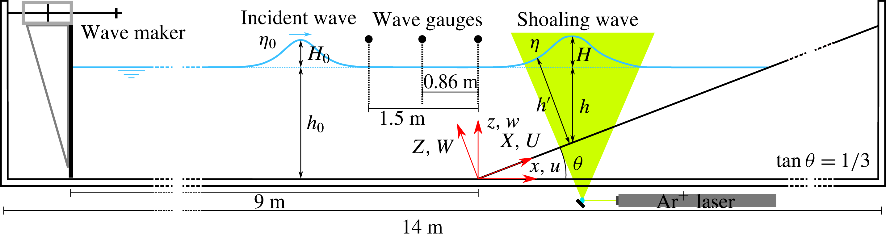
Figure 1. Schematic diagram of the experimental set-up in the wave flume with a 1 : 3 sloping bottom.
Two Cartesian coordinate systems, defined in figure 1, will be used in this paper. The origins of both coordinate systems are located at the toe of the sloping bottom along the centreline of the wave flume. The
 $x$
-axis is the horizontal coordinate in the longitudinal direction, pointing positively in the direction of wave propagation. The
$x$
-axis is the horizontal coordinate in the longitudinal direction, pointing positively in the direction of wave propagation. The
 $y$
-axis is the spanwise horizontal coordinate and is perpendicular to the
$y$
-axis is the spanwise horizontal coordinate and is perpendicular to the
 $x$
-axis. Finally, the
$x$
-axis. Finally, the
 $z$
-axis is the vertical coordinate, pointing upwards and measuring from the horizontal bottom. The second coordinate system
$z$
-axis is the vertical coordinate, pointing upwards and measuring from the horizontal bottom. The second coordinate system
 $(X,Y,Z)$
is obtained by rotating
$(X,Y,Z)$
is obtained by rotating
 $(x,y,z)$
by an angle of
$(x,y,z)$
by an angle of
 $18.43^{\circ }$
on the
$18.43^{\circ }$
on the
 $x$
–
$x$
–
 $z$
plane so that the positive
$z$
plane so that the positive
 $X$
-axis is oriented shorewards along the surface of the sloping bottom. Therefore, the
$X$
-axis is oriented shorewards along the surface of the sloping bottom. Therefore, the
 $Z$
-axis is perpendicular to the slope, pointing up into the water body. As shown in figure 1,
$Z$
-axis is perpendicular to the slope, pointing up into the water body. As shown in figure 1,
 $\unicode[STIX]{x1D702}$
denotes the instantaneous free-surface elevation in the
$\unicode[STIX]{x1D702}$
denotes the instantaneous free-surface elevation in the
 $(x,y,z)$
coordinate system.
$(x,y,z)$
coordinate system.
 $h$
and
$h$
and
 $h^{\prime }$
are the still-water depth in the
$h^{\prime }$
are the still-water depth in the
 $(x,y,z)$
coordinate system and the total water depth in the coordinate system
$(x,y,z)$
coordinate system and the total water depth in the coordinate system
 $(X,Y,Z)$
, respectively. Finally, the associated velocity components defined in the
$(X,Y,Z)$
, respectively. Finally, the associated velocity components defined in the
 $(x,y,z)$
and
$(x,y,z)$
and
 $(X,Y,Z)$
coordinates are
$(X,Y,Z)$
coordinates are
 $(u,v,w)$
and
$(u,v,w)$
and
 $(U,V,W)$
. Herein,
$(U,V,W)$
. Herein,
 $t$
denotes time and the corresponding non-dimensional time is defined as
$t$
denotes time and the corresponding non-dimensional time is defined as
 $T=t\sqrt{g/h_{0}}$
, where
$T=t\sqrt{g/h_{0}}$
, where
 $h_{0}$
is the still-water depth in the constant-depth region (see figure 1). We remark here that in the experiments
$h_{0}$
is the still-water depth in the constant-depth region (see figure 1). We remark here that in the experiments
 $t=0$
s (also
$t=0$
s (also
 $T=0$
) denotes the instant when the crest of the solitary wave is above the toe of the sloping bottom, i.e. at
$T=0$
) denotes the instant when the crest of the solitary wave is above the toe of the sloping bottom, i.e. at
 $x=0$
(also at
$x=0$
(also at
 $X=0$
).
$X=0$
).
The free-surface elevations were measured with capacitance-type wave gauges. The first gauge was located at
 $x=-1.50~\text{m}$
and the second at
$x=-1.50~\text{m}$
and the second at
 $x=0.00~\text{m}$
(the toe of the slope) along the centreline of the flume. A third wave gauge at
$x=0.00~\text{m}$
(the toe of the slope) along the centreline of the flume. A third wave gauge at
 $x=-0.86~\text{m}$
was also available for some experimental runs. The first wave gauge is sufficiently far away from the wave maker and the slope, therefore, the measured time series of free-surface elevation
$x=-0.86~\text{m}$
was also available for some experimental runs. The first wave gauge is sufficiently far away from the wave maker and the slope, therefore, the measured time series of free-surface elevation
 $\unicode[STIX]{x1D702}_{0}(t)$
and the wave height
$\unicode[STIX]{x1D702}_{0}(t)$
and the wave height
 $H_{0}$
are viewed as the incident solitary wave propagating over horizontal bottom. The voltage output of this gauge was also used as a reference signal to trigger the HSPIV (high speed particle image velocimetry) for velocity measurements. The second wave gauge is used to set the initial time
$H_{0}$
are viewed as the incident solitary wave propagating over horizontal bottom. The voltage output of this gauge was also used as a reference signal to trigger the HSPIV (high speed particle image velocimetry) for velocity measurements. The second wave gauge is used to set the initial time
 $t=0~\text{s}$
.
$t=0~\text{s}$
.
The solitary wave was generated according to Goring (Reference Goring1978). The wave height of
 $H_{0}=2.9~\text{cm}$
was produced in a constant water depth of
$H_{0}=2.9~\text{cm}$
was produced in a constant water depth of
 $h_{0}=8.0~\text{cm}$
, resulting in a nonlinearity of
$h_{0}=8.0~\text{cm}$
, resulting in a nonlinearity of
 $H_{0}/h_{0}=0.363$
.
$H_{0}/h_{0}=0.363$
.
2.2 Flow visualization technique
A flow visualization technique, using the particle trajectory method, was employed in this study. The aims are to explore temporal and spatial variations of the free-surface profile, and to visualize the flow structure underneath the free surface during the runup and rundown phases. Titanium dioxide (
 $\text{TiO}_{2}$
) particles with a refractive index of 2.6 and a mean diameter of
$\text{TiO}_{2}$
) particles with a refractive index of 2.6 and a mean diameter of
 $1.8~\unicode[STIX]{x03BC}\text{m}$
were used as seeding particles. The fall velocity (or settling velocity) of these particles was
$1.8~\unicode[STIX]{x03BC}\text{m}$
were used as seeding particles. The fall velocity (or settling velocity) of these particles was
 $4.5\times 10^{-4}~\text{cm}~\text{s}^{-1}$
, estimated by Stokes’ law.
$4.5\times 10^{-4}~\text{cm}~\text{s}^{-1}$
, estimated by Stokes’ law.
A high-speed digital camera was employed to capture particle motions. This camera (Phantom M310, Vision Research) has the ability to capture images with a maximum framing rate of 3260 Hz under the largest resolution of
 $1280~\text{pixel}\times 800~\text{pixel}$
with a 12-bit dynamic range.
$1280~\text{pixel}\times 800~\text{pixel}$
with a 12-bit dynamic range.
A laser light sheet was used to illuminate the 2D motion of suspended particles in a vertical plane. An argon-ion laser head (Innova-300, Coherent Inc.) with 7 W maximum energy output was used as a light source. A combination of reflection mirrors and optical lenses was deployed to divert the laser beam into a fan-shaped light sheet with a thickness of approximately 1.5 mm. The laser light sheet was then projected upwards through the centreline of glass bottom of the wave flume (see figure 1).
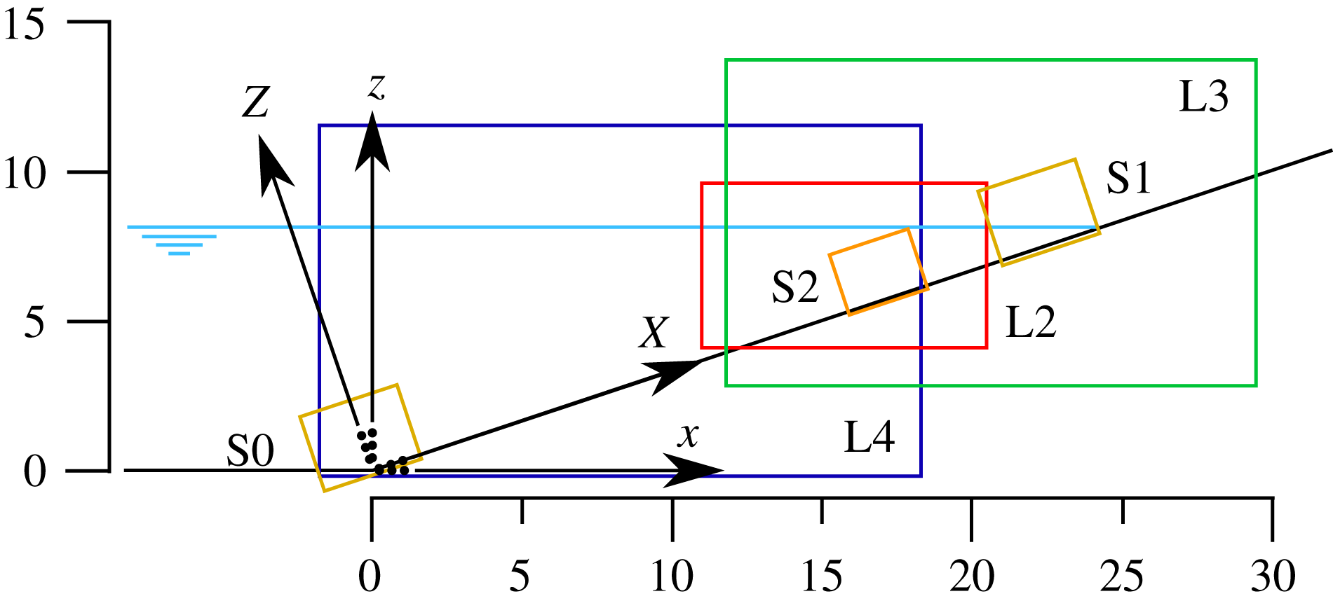
Figure 2. Reference sketch for the fields of view (FOV) for flow feature visualization and HSPIV. Units are in cm. Exact FOV locations are referenced in table 1.
Table 1. Locations of the FOVs shown in figure 2. Resolution in number of velocity measurements per cm.
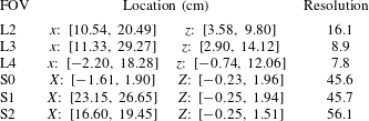
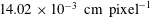
To track the rapid variation in the free-surface profile, the camera was operated at a framing rate of 2000 Hz for the fields of view L2–L4 shown in figure 2. The spatial resolution varies between
 $7.77\times 10^{-3}~\text{cm}~\text{pixel}^{-1}$
and
$7.77\times 10^{-3}~\text{cm}~\text{pixel}^{-1}$
and
 $14.02\times 10^{-3}~\text{cm}~\text{pixel}^{-1}$
, or between
$14.02\times 10^{-3}~\text{cm}~\text{pixel}^{-1}$
, or between
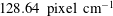 $128.64~\text{pixel}~\text{cm}^{-1}$
and
$128.64~\text{pixel}~\text{cm}^{-1}$
and
 $62.5~\text{pixel}~\text{cm}^{-1}$
. As the free surface acts like a mirror, reflecting the laser light sheet projected from below the flume bottom, the location of the free surface is obtained by manually fitting a curve to the bright profile in the images.
$62.5~\text{pixel}~\text{cm}^{-1}$
. As the free surface acts like a mirror, reflecting the laser light sheet projected from below the flume bottom, the location of the free surface is obtained by manually fitting a curve to the bright profile in the images.
Alternatively, to explore the ‘pathline’ pattern of the flow structure under the free surface, the sampling rate of the camera was set at 200 Hz–
 $500~\text{Hz}$
, depending on the size of the observation area needed. Since the shutter speed of the camera is relatively low, the particles reflecting the bright laser light imprint the pathlines contrasting with the dark background. Particles moving faster trace longer curves, while those with velocities close to zero appear as points. Therefore, the flow visualization technique can be applied to identify flow features and to measure their length scales.
$500~\text{Hz}$
, depending on the size of the observation area needed. Since the shutter speed of the camera is relatively low, the particles reflecting the bright laser light imprint the pathlines contrasting with the dark background. Particles moving faster trace longer curves, while those with velocities close to zero appear as points. Therefore, the flow visualization technique can be applied to identify flow features and to measure their length scales.
2.3 Velocity measurements by HSPIV
The laser head, detailed deployment of reflection mirrors and optical lens, and the seeding particles used for the HSPIV system are the same as those employed in the flow visualization technique described above. To allow high image resolution and appropriate magnification of the measuring area, a Nikon 200 mm lens (f/4.0D AF Micro-Nikkor) was fitted to the camera. The images of flow fields characterized by the movement of suspended particles are continuously recorded by using the camera with a controlled exposure time between
 $10~\unicode[STIX]{x03BC}\text{s}$
and
$10~\unicode[STIX]{x03BC}\text{s}$
and
 $47\,000~\unicode[STIX]{x03BC}\text{s}$
. To ensure a high time-resolved HSPIV algorithm, a framing rate of 2000 Hz for the camera was set while capturing the images of the velocity fields.
$47\,000~\unicode[STIX]{x03BC}\text{s}$
. To ensure a high time-resolved HSPIV algorithm, a framing rate of 2000 Hz for the camera was set while capturing the images of the velocity fields.
To investigate the time variation of the velocity field over the sloping bottom, six fields of view (shown in figure 2) were employed. The widest FOVs (L3 and L4) provide a resolution of
 $14.02\times 10^{-3}~\text{cm}~\text{pixel}^{-1}$
in the
$14.02\times 10^{-3}~\text{cm}~\text{pixel}^{-1}$
in the
 $x$
and
$x$
and
 $z$
directions, while L2 provides a resolution of
$z$
directions, while L2 provides a resolution of
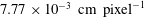 $7.77\times 10^{-3}~\text{cm}~\text{pixel}^{-1}$
. For measuring the detailed velocity field close to the sloping bottom, the FOVs S0 and S1 provide a higher resolution of
$7.77\times 10^{-3}~\text{cm}~\text{pixel}^{-1}$
. For measuring the detailed velocity field close to the sloping bottom, the FOVs S0 and S1 provide a higher resolution of
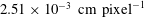 $2.51\times 10^{-3}~\text{cm}~\text{pixel}^{-1}$
in the
$2.51\times 10^{-3}~\text{cm}~\text{pixel}^{-1}$
in the
 $x$
and
$x$
and
 $z$
directions, and FOV S2 provides the highest resolution of
$z$
directions, and FOV S2 provides the highest resolution of
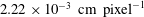 $2.22\times 10^{-3}~\text{cm}~\text{pixel}^{-1}$
.
$2.22\times 10^{-3}~\text{cm}~\text{pixel}^{-1}$
.
The PIV analysis is performed with an in-house code. Before performing the cross-correlation calculation for the velocity field, the Laplacian edge-enhancement technique (Adrian & Westerweel Reference Adrian and Westerweel2011) and the hybrid digital particle-tracking velocimetry technique (Cowen & Monismith Reference Cowen and Monismith1997) are adopted for the contrast enhancement of particle-laden images captured by the high-speed camera. The images obtained are then subtracted from the background images to remove any constant noise source. The multi-pass PIV algorithm calculates the instantaneous velocity field from a pair of images starting from the interrogation window size of
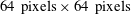 $64~\text{pixels}\times 64~\text{pixels}$
, ending with a smaller window size of
$64~\text{pixels}\times 64~\text{pixels}$
, ending with a smaller window size of
 $8~\text{pixels}\times 8~\text{pixels}$
with a 50 % overlap for the FOV. Both global range and median filters are used to remove spurious vectors. Consequential missing vectors are then interpolated to construct the whole-field velocity vectors. Under these conditions the spatial resolution for velocity vectors ranges from 0.18 mm to 1.1 mm, depending on the FOV, as shown in table 1.
$8~\text{pixels}\times 8~\text{pixels}$
with a 50 % overlap for the FOV. Both global range and median filters are used to remove spurious vectors. Consequential missing vectors are then interpolated to construct the whole-field velocity vectors. Under these conditions the spatial resolution for velocity vectors ranges from 0.18 mm to 1.1 mm, depending on the FOV, as shown in table 1.
The magnitude of errors for the HSPIV technique is estimated with the following method (Chang & Liu Reference Chang and Liu2000; Lin et al.
Reference Lin, Hseih, Lin, Chang and Raikar2012, Reference Lin, Yeh, Kao, Yu, Hseih, Chang, Wu and Tsai2015b
). The largest velocity gradients near the sloping bottom measured in FOV L2 are
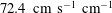 $72.4~\text{cm}~\text{s}^{-1}~\text{cm}^{-1}$
(for a free-stream velocity of
$72.4~\text{cm}~\text{s}^{-1}~\text{cm}^{-1}$
(for a free-stream velocity of
 $38.0~\text{cm}~\text{s}^{-1}$
, at
$38.0~\text{cm}~\text{s}^{-1}$
, at
 $t=0.18~\text{s}$
and
$t=0.18~\text{s}$
and
 $x=19.0~\text{cm}$
) and
$x=19.0~\text{cm}$
) and
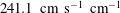 $241.1~\text{cm}~\text{s}^{-1}~\text{cm}^{-1}$
(for a free-stream velocity of
$241.1~\text{cm}~\text{s}^{-1}~\text{cm}^{-1}$
(for a free-stream velocity of
 $106.0~\text{cm}~\text{s}^{-1}$
, at
$106.0~\text{cm}~\text{s}^{-1}$
, at
 $t=1.05~\text{s}$
and
$t=1.05~\text{s}$
and
 $x=19.0~\text{cm}$
), for the runup and rundown phases of the solitary wave, respectively. Since the framing rate was set to 2000 Hz, the corresponding uncertainties are approximately 0.080 pixel and 0.205 pixel, respectively (Keane & Adrian Reference Keane and Adrian1992). The estimated errors of the horizontal component of velocity (
$x=19.0~\text{cm}$
), for the runup and rundown phases of the solitary wave, respectively. Since the framing rate was set to 2000 Hz, the corresponding uncertainties are approximately 0.080 pixel and 0.205 pixel, respectively (Keane & Adrian Reference Keane and Adrian1992). The estimated errors of the horizontal component of velocity (
 $u$
) are equal to
$u$
) are equal to
 $1.25~\text{cm}~\text{s}^{-1}$
[
$1.25~\text{cm}~\text{s}^{-1}$
[
 $=0.080~\text{pixel}\times 0.0078~\text{cm}~\text{pixel}^{-1}\times 2000~~\text{s}^{-1}$
] and
$=0.080~\text{pixel}\times 0.0078~\text{cm}~\text{pixel}^{-1}\times 2000~~\text{s}^{-1}$
] and
 $3.20~\text{cm}~\text{s}^{-1}$
[
$3.20~\text{cm}~\text{s}^{-1}$
[
 $=0.205~\text{pixel}\times 0.0078~\text{cm}~\text{pixel}^{-1}\times 2000~\text{s}^{-1}$
] for the runup and rundown phases. In both cases, the relative errors in terms of the free-stream velocities near the free surface are approximately 3 %.
$=0.205~\text{pixel}\times 0.0078~\text{cm}~\text{pixel}^{-1}\times 2000~\text{s}^{-1}$
] for the runup and rundown phases. In both cases, the relative errors in terms of the free-stream velocities near the free surface are approximately 3 %.
Similarly, the largest velocity gradients measured in the boundary layer of FOV S1 are
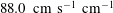 $88.0~\text{cm}~\text{s}^{-1}~\text{cm}^{-1}$
(for a free-stream velocity of
$88.0~\text{cm}~\text{s}^{-1}~\text{cm}^{-1}$
(for a free-stream velocity of
 $45.0~\text{cm}~\text{s}^{-1}$
, at
$45.0~\text{cm}~\text{s}^{-1}$
, at
 $t=0.18~\text{s}$
and
$t=0.18~\text{s}$
and
 $x=24.0~\text{cm}$
) and
$x=24.0~\text{cm}$
) and
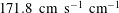 $171.8~\text{cm}~\text{s}^{-1}~\text{cm}^{-1}$
(for a free-stream velocity of
$171.8~\text{cm}~\text{s}^{-1}~\text{cm}^{-1}$
(for a free-stream velocity of
 $88.0~\text{cm}~\text{s}^{-1}$
, at
$88.0~\text{cm}~\text{s}^{-1}$
, at
 $t=0.96~\text{s}$
and
$t=0.96~\text{s}$
and
 $x=22.5~\text{cm}$
) for the runup and rundown phases. The uncertainties are approximately 0.070 pixel and 0.100 pixel, for a framing rate of 3000 Hz in this case. The estimated errors in
$x=22.5~\text{cm}$
) for the runup and rundown phases. The uncertainties are approximately 0.070 pixel and 0.100 pixel, for a framing rate of 3000 Hz in this case. The estimated errors in
 $u$
for FOV S1 are
$u$
for FOV S1 are
 $0.57~\text{cm}~\text{s}^{-1}$
[
$0.57~\text{cm}~\text{s}^{-1}$
[
 $=0.070~\text{pixel}\times 0.0027~\text{cm}~\text{pixel}^{-1}\times 3000~\text{s}^{-1}$
] and
$=0.070~\text{pixel}\times 0.0027~\text{cm}~\text{pixel}^{-1}\times 3000~\text{s}^{-1}$
] and
 $0.81~\text{cm}~\text{s}^{-1}$
[
$0.81~\text{cm}~\text{s}^{-1}$
[
 $=0.100~\text{pixel}\times 0.0027~\text{cm}~\text{pixel}^{-1}\times 3000~\text{s}^{-1}$
] for the runup and rundown phases, respectively. The relative errors in terms of the free-stream velocities at the edge of the boundary layer are below 1.3 %.
$=0.100~\text{pixel}\times 0.0027~\text{cm}~\text{pixel}^{-1}\times 3000~\text{s}^{-1}$
] for the runup and rundown phases, respectively. The relative errors in terms of the free-stream velocities at the edge of the boundary layer are below 1.3 %.
In this study HSPIV and laser Doppler velocimetry (LDV) measurements of the horizontal velocity profile for the solitary wave in a constant depth were also compared. The LDV data compare very well with the HSPIV measurements at several different times (or phases) inside and outside the bottom boundary layer. In this paper we shall report only the HSPIV measurements.
2.4 Experimental observations
During the experiments the free-surface elevation profile measured in the constant-water-depth region (
 $x=-1.50~\text{m}$
) was found to match reasonably well with the theoretical solitary wave profile in Boussinesq (Reference Boussinesq1872). Moreover, the solitary wave did not break during the shoaling and runup phases. This observation is in agreement with the wave breaking criteria for solitary waves, based on numerical experiments by Grilli, Svendsen & Subramanya (Reference Grilli, Svendsen and Subramanya1997).
$x=-1.50~\text{m}$
) was found to match reasonably well with the theoretical solitary wave profile in Boussinesq (Reference Boussinesq1872). Moreover, the solitary wave did not break during the shoaling and runup phases. This observation is in agreement with the wave breaking criteria for solitary waves, based on numerical experiments by Grilli, Svendsen & Subramanya (Reference Grilli, Svendsen and Subramanya1997).
A total of 10 repeated runs were performed to assess repeatability for the free-surface profile and HSPIV measurements. All 10 repetitions yield virtually identical free-surface profiles and velocities. The analysis of 17 transects yields minimum and maximum standard deviations for free-surface elevations of 0 pixel and 0.98 pixel. Since the resolution of the images (FOVs L3 and L4) is
 $14.02\times 10^{-3}~\text{cm}~\text{pixel}^{-1}$
, the global mean of the standard deviations is
$14.02\times 10^{-3}~\text{cm}~\text{pixel}^{-1}$
, the global mean of the standard deviations is
 $7\times 10^{-3}~\text{cm}$
(0.55 pixel). Repeated runs were averaged to eliminate small fluctuations from the velocity time series, on the order of 1 %–3 % of the free-stream velocity, which may arise from the HSPIV measurement errors. Therefore, from here on, the experimental results presented in this paper are an ensemble average of 10 runs.
$7\times 10^{-3}~\text{cm}$
(0.55 pixel). Repeated runs were averaged to eliminate small fluctuations from the velocity time series, on the order of 1 %–3 % of the free-stream velocity, which may arise from the HSPIV measurement errors. Therefore, from here on, the experimental results presented in this paper are an ensemble average of 10 runs.
The measured and calculated values of wave celerity,
 $c_{0}$
, defined as
$c_{0}$
, defined as
 $\sqrt{g(H_{0}+h_{0})}$
, are
$\sqrt{g(H_{0}+h_{0})}$
, are
 $102.0~\text{cm}~\text{s}^{-1}$
and
$102.0~\text{cm}~\text{s}^{-1}$
and
 $103.4~\text{cm}~\text{s}^{-1}$
, respectively, yielding a relative error smaller than 1.4 %. Note that the non-dimensional form of the measured wave celerity is
$103.4~\text{cm}~\text{s}^{-1}$
, respectively, yielding a relative error smaller than 1.4 %. Note that the non-dimensional form of the measured wave celerity is
 $c_{0}/\sqrt{g(H_{0}+h_{0})}$
, and is equal to 0.99.
$c_{0}/\sqrt{g(H_{0}+h_{0})}$
, and is equal to 0.99.
The Reynolds number for a solitary wave (applicable in the uprush phase) can be defined as (Sumer et al.
Reference Sumer, Jensen, Sørensen, Fredsøe, Liu and Carstensen2010):
 $Re_{u}=a(u_{\infty })_{max}/\unicode[STIX]{x1D708}$
, in which
$Re_{u}=a(u_{\infty })_{max}/\unicode[STIX]{x1D708}$
, in which
 $\unicode[STIX]{x1D708}$
is the kinematic viscosity of water,
$\unicode[STIX]{x1D708}$
is the kinematic viscosity of water,
 $a$
is the amplitude (or half of the stroke) of the water particle displacement in the free-stream region and
$a$
is the amplitude (or half of the stroke) of the water particle displacement in the free-stream region and
 $(u_{\infty })_{max}$
is the maximum free-stream velocity. For the present case with
$(u_{\infty })_{max}$
is the maximum free-stream velocity. For the present case with
 $H_{0}/h_{0}=0.363$
, the maximum Reynolds number at the slope during the runup phase (wave-driven flow) can be calculated as 11 000, which is within the laminar flow regime (Sumer et al.
Reference Sumer, Jensen, Sørensen, Fredsøe, Liu and Carstensen2010). During rundown, the flow is gravity-driven, therefore it is assimilated with open channel flow and the Reynolds number is calculated with the hydraulic radius instead:
$H_{0}/h_{0}=0.363$
, the maximum Reynolds number at the slope during the runup phase (wave-driven flow) can be calculated as 11 000, which is within the laminar flow regime (Sumer et al.
Reference Sumer, Jensen, Sørensen, Fredsøe, Liu and Carstensen2010). During rundown, the flow is gravity-driven, therefore it is assimilated with open channel flow and the Reynolds number is calculated with the hydraulic radius instead:
 $Re_{d}=r_{h}~(u_{\infty })_{max}/\unicode[STIX]{x1D708}$
. (The hydraulic radius (
$Re_{d}=r_{h}~(u_{\infty })_{max}/\unicode[STIX]{x1D708}$
. (The hydraulic radius (
 $r_{h}$
) is defined as two times the cross-sectional area of the flow divided by the wetted perimeter of the cross-section. During the later rundown phase the flow is very shallow compared to the width of the flume, therefore
$r_{h}$
) is defined as two times the cross-sectional area of the flow divided by the wetted perimeter of the cross-section. During the later rundown phase the flow is very shallow compared to the width of the flume, therefore
 $r_{h}\simeq h^{\prime }$
.) The downrush flow is initially laminar (
$r_{h}\simeq h^{\prime }$
.) The downrush flow is initially laminar (
 $Re_{d}<500$
), since this phase starts from a near-rest situation. As rundown progresses, the flow at the slope accelerates and transitions from a laminar to a turbulent regime. The maximum Reynolds number obtained during rundown is 30 000 along the thin downrush flow before the hydraulic jump overturns, which is already turbulent (
$Re_{d}<500$
), since this phase starts from a near-rest situation. As rundown progresses, the flow at the slope accelerates and transitions from a laminar to a turbulent regime. The maximum Reynolds number obtained during rundown is 30 000 along the thin downrush flow before the hydraulic jump overturns, which is already turbulent (
 $Re_{d}>12\,500$
). Scaling up the physical dimension of the present case to a field condition by a factor of 100 (the still-water depth becomes 8 m) would increase the Reynolds number by three orders of magnitude, which will be far beyond the laminar and low-turbulence regime studied in this paper. Therefore, we stress that the present study focuses only on the swash flow at a laboratory scale.
$Re_{d}>12\,500$
). Scaling up the physical dimension of the present case to a field condition by a factor of 100 (the still-water depth becomes 8 m) would increase the Reynolds number by three orders of magnitude, which will be far beyond the laminar and low-turbulence regime studied in this paper. Therefore, we stress that the present study focuses only on the swash flow at a laboratory scale.
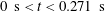
2.4.1 Time evolution of free-surface profiles

Figure 3. Timeline for the different physical processes (e.g. shoaling, runup, rundown, flow separation) in the swash flow generated by a non-breaking solitary wave (
 $H_{0}/h_{0}=0.363$
) on a steep (1 : 3) slope. Top part: experiments. Bottom part: numerical simulation. The dashed lines link the time of occurrence of the physical processes in the experiment/simulation. Locations of the physical processes (if applicable) are provided in the text boxes. Experimental times have been rounded to the closest 1/100 s to match the output time rate of the numerical simulation.
$H_{0}/h_{0}=0.363$
) on a steep (1 : 3) slope. Top part: experiments. Bottom part: numerical simulation. The dashed lines link the time of occurrence of the physical processes in the experiment/simulation. Locations of the physical processes (if applicable) are provided in the text boxes. Experimental times have been rounded to the closest 1/100 s to match the output time rate of the numerical simulation.

Figure 4. Snapshots of laboratory observed free-surface profiles during runup and rundown phases of a solitary wave with
 $H_{0}/h_{0}=0.363$
and
$H_{0}/h_{0}=0.363$
and
 $h_{0}=8~\text{cm}$
. (a) Runup. (b) Rundown.
$h_{0}=8~\text{cm}$
. (a) Runup. (b) Rundown.
Based on the experimental observations, the timeline of evolution of a non-breaking solitary wave (
 $H_{0}/h_{0}=0.363$
) propagating over a 1 in 3 slope is displayed in figure 3. The swash of a solitary wave comprises four phases: wave shoaling, runup flow, rundown flow and hydraulic jump, included in the timeline. Only the experimental (top) timeline will be discussed next. The numerical simulation timeline is slightly different from the experimental one and will be addressed in §§ 3.4 and 4.
$H_{0}/h_{0}=0.363$
) propagating over a 1 in 3 slope is displayed in figure 3. The swash of a solitary wave comprises four phases: wave shoaling, runup flow, rundown flow and hydraulic jump, included in the timeline. Only the experimental (top) timeline will be discussed next. The numerical simulation timeline is slightly different from the experimental one and will be addressed in §§ 3.4 and 4.
At time
 $t=0~\text{s}$
, the wave crest was located at the toe of the slope. During the time interval,
$t=0~\text{s}$
, the wave crest was located at the toe of the slope. During the time interval,
 $-0.473~\text{s}<t<0.654~\text{s}$
, the solitary wave first shoaled and soon started the runup phase. The snapshots of observed free-surface profiles at five instants are plotted in figure 4(a). During the shoaling phase (
$-0.473~\text{s}<t<0.654~\text{s}$
, the solitary wave first shoaled and soon started the runup phase. The snapshots of observed free-surface profiles at five instants are plotted in figure 4(a). During the shoaling phase (
 $-0.473~\text{s}<t<0.271~\text{s}$
), the wave crest can be identified, while in the runup phase the vertical elevation of the moving shoreline (runup height) was the highest elevation of the entire flow domain. The shoreline moved continuously upwards on the slope, forming a thin layer of swash flow. Near the shoreline the free surface bent into the direction normal to the slope, displaying the meniscus. The maximum runup height was reached at
$-0.473~\text{s}<t<0.271~\text{s}$
), the wave crest can be identified, while in the runup phase the vertical elevation of the moving shoreline (runup height) was the highest elevation of the entire flow domain. The shoreline moved continuously upwards on the slope, forming a thin layer of swash flow. Near the shoreline the free surface bent into the direction normal to the slope, displaying the meniscus. The maximum runup height was reached at
 $t=0.654~\text{s}$
, and afterwards the shoreline started to retreat, as shown in figure 4(b).
$t=0.654~\text{s}$
, and afterwards the shoreline started to retreat, as shown in figure 4(b).
The rundown phase covered the time interval
 $0.654~\text{s}<t<1.217~\text{s}$
(see figure 3). During this period the water depth in the entire swash zone decreased monotonically. It is pointed out here that the free-surface elevation at
$0.654~\text{s}<t<1.217~\text{s}$
(see figure 3). During this period the water depth in the entire swash zone decreased monotonically. It is pointed out here that the free-surface elevation at
 $x=13~\text{cm}$
remained more or less constant (near the still-water level) for
$x=13~\text{cm}$
remained more or less constant (near the still-water level) for
 $0.654~\text{s}<t<1.056~\text{s}$
(see figure 4
b). The rundown flows were driven by gravity and the accelerating flow ran into a large and almost stationary water body. This flow condition led to the development of a hydraulic jump at
$0.654~\text{s}<t<1.056~\text{s}$
(see figure 4
b). The rundown flows were driven by gravity and the accelerating flow ran into a large and almost stationary water body. This flow condition led to the development of a hydraulic jump at
 $t=1.007~\text{s}$
, when the free surface became almost vertical at
$t=1.007~\text{s}$
, when the free surface became almost vertical at
 $x=14.6~\text{cm}$
. The free surface eventually curled over towards the shore (as shown by the profile at
$x=14.6~\text{cm}$
. The free surface eventually curled over towards the shore (as shown by the profile at
 $t=1.056~\text{s}$
in figure 4) and impinged on the fast incoming (downrush) flow. A significant amount of air bubbles were entrained into the water body.
$t=1.056~\text{s}$
in figure 4) and impinged on the fast incoming (downrush) flow. A significant amount of air bubbles were entrained into the water body.
2.4.2 Time evolution of velocity field
The time evolution of the velocity field is analysed in figures 5–9. The number of velocity vectors has been downsampled in the
 $x$
and
$x$
and
 $z$
directions from the original values (see table 1) for visual clarity, as indicated in the captions.
$z$
directions from the original values (see table 1) for visual clarity, as indicated in the captions.
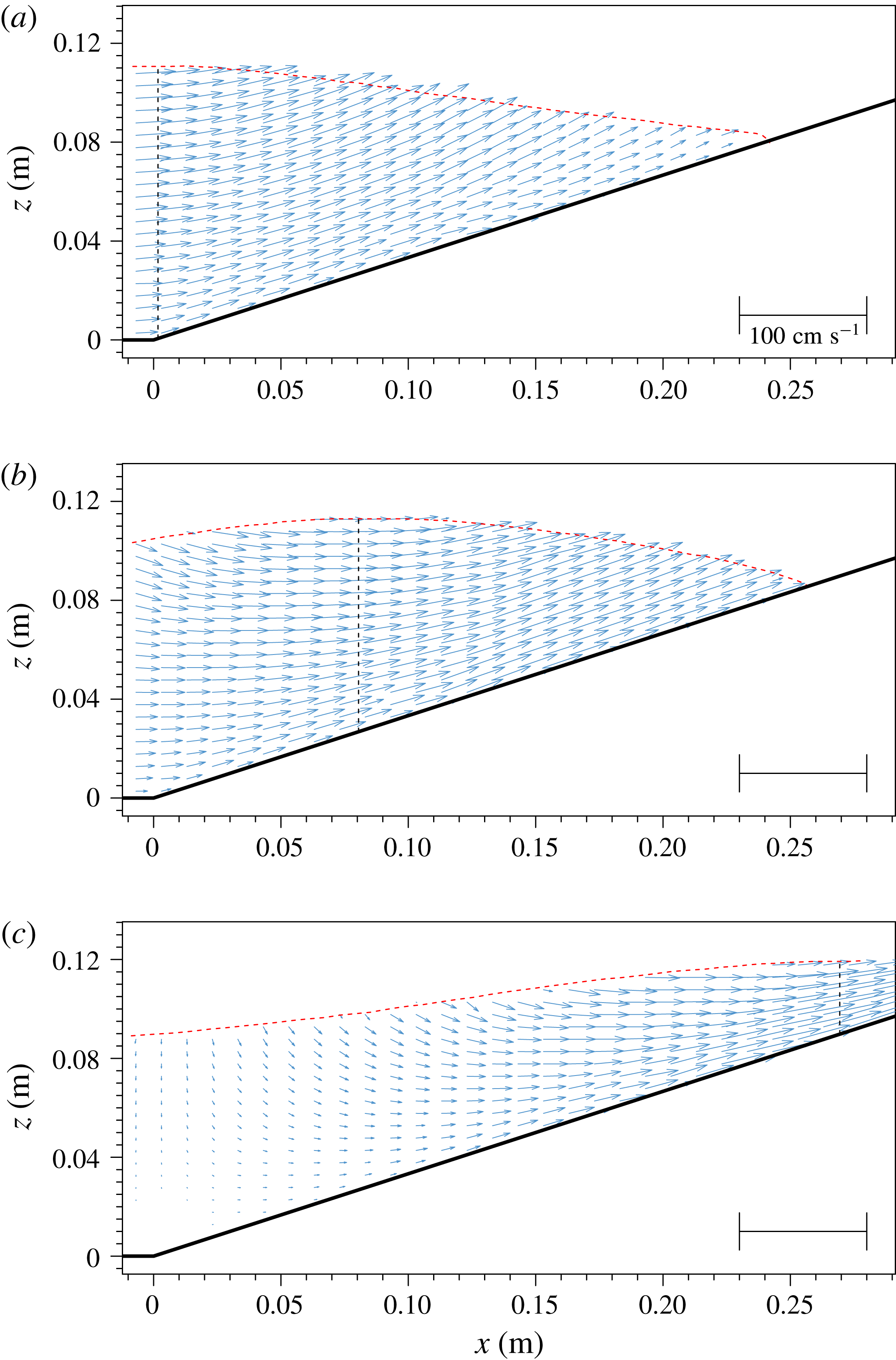
Figure 5. Snapshots of free-surface elevation (red dashed line) and measured velocity fields for
 $-1~\text{cm}<x<28~\text{cm}$
and
$-1~\text{cm}<x<28~\text{cm}$
and
 $0~\text{s}<t<0.271~\text{s}$
, during the shoaling phase. The vertical dashed line indicates the location of the wave crest. Experimental data have been downsampled to 1 and 2 arrows
$0~\text{s}<t<0.271~\text{s}$
, during the shoaling phase. The vertical dashed line indicates the location of the wave crest. Experimental data have been downsampled to 1 and 2 arrows
 $\text{cm}^{-1}$
in the horizontal and vertical directions, respectively. (a)
$\text{cm}^{-1}$
in the horizontal and vertical directions, respectively. (a)
 $t=0~\text{s}$
, (b)
$t=0~\text{s}$
, (b)
 $t=0.090~\text{s}$
and (c)
$t=0.090~\text{s}$
and (c)
 $t=0.271~\text{s}$
.
$t=0.271~\text{s}$
.
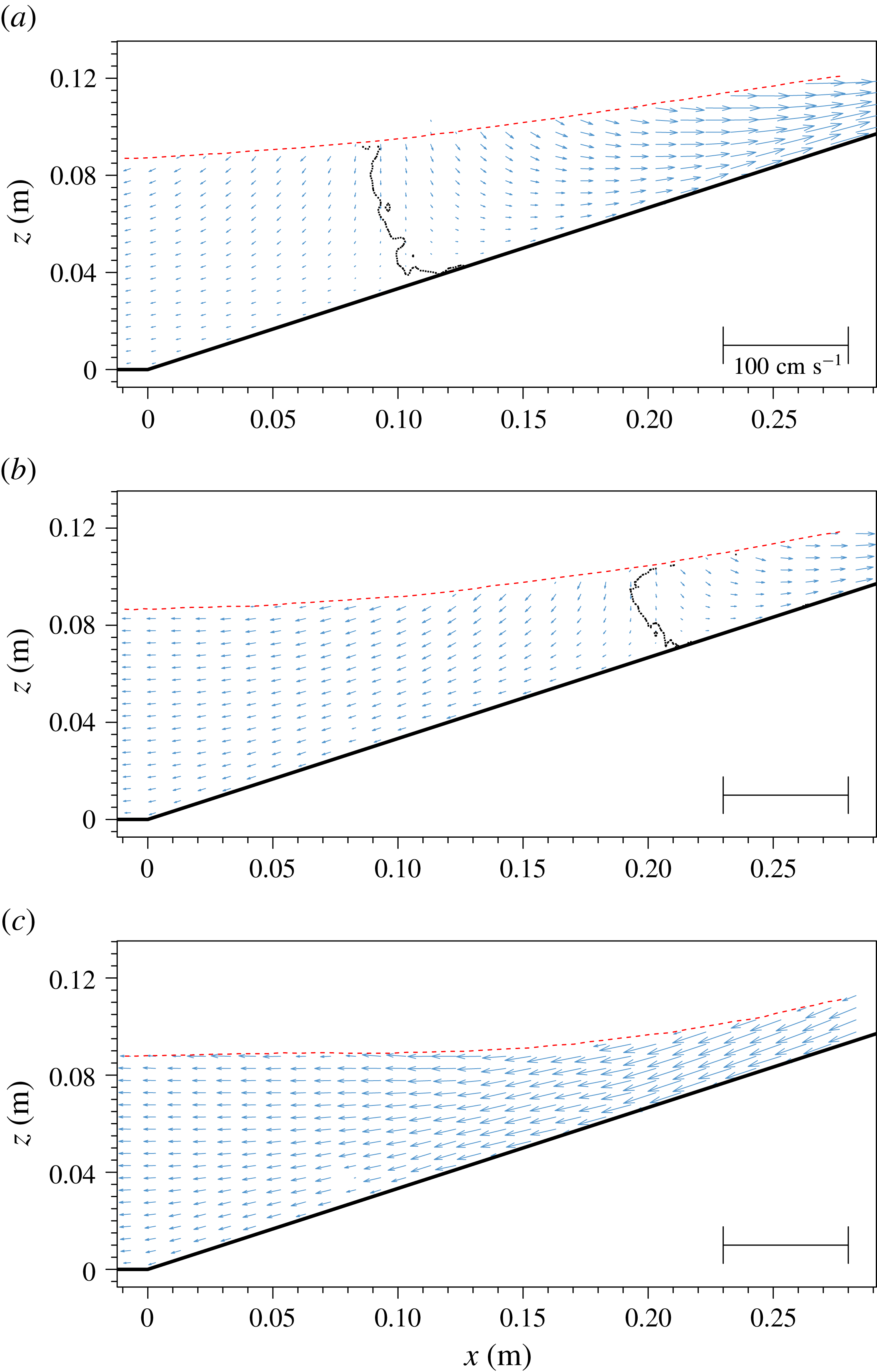
Figure 6. Velocity field measured for
 $-1~\text{cm}<x<28~\text{cm}$
and
$-1~\text{cm}<x<28~\text{cm}$
and
 $0.361~\text{s}<t<0.632~\text{s}$
, during the runup phase. The dotted curves trace the zero horizontal velocity locations. These curves divide the shoreward flow field and seaward flow field. Experimental data have been downsampled to 1 and 2 arrows
$0.361~\text{s}<t<0.632~\text{s}$
, during the runup phase. The dotted curves trace the zero horizontal velocity locations. These curves divide the shoreward flow field and seaward flow field. Experimental data have been downsampled to 1 and 2 arrows
 $\text{cm}^{-1}$
in the horizontal and vertical directions, respectively. (a)
$\text{cm}^{-1}$
in the horizontal and vertical directions, respectively. (a)
 $t=0.361~\text{s}$
, (b)
$t=0.361~\text{s}$
, (b)
 $t=0.452~\text{s}$
and (c)
$t=0.452~\text{s}$
and (c)
 $t=0.632~\text{s}$
.
$t=0.632~\text{s}$
.
Figure 7. The zoom-in view of velocity fields for
 $23.4~\text{cm}<X<26.1~\text{cm}$
and
$23.4~\text{cm}<X<26.1~\text{cm}$
and
 $0.361~\text{s}<t<0.632~\text{s}$
, during the flow reversal course throughout the runup phase. The dotted curves trace the zero horizontal velocity locations, dividing the shoreward flow field and seaward flow field. Experimental data have been downsampled in the horizontal direction only, to 5 arrows
$0.361~\text{s}<t<0.632~\text{s}$
, during the flow reversal course throughout the runup phase. The dotted curves trace the zero horizontal velocity locations, dividing the shoreward flow field and seaward flow field. Experimental data have been downsampled in the horizontal direction only, to 5 arrows
 $\text{cm}^{-1}$
. (a)
$\text{cm}^{-1}$
. (a)
 $t=0.361~\text{s}$
, (b)
$t=0.361~\text{s}$
, (b)
 $t=0.406~\text{s}$
, (c)
$t=0.406~\text{s}$
, (c)
 $t=0.452~\text{s}$
, (d)
$t=0.452~\text{s}$
, (d)
 $t=0.474~\text{s}$
, (e)
$t=0.474~\text{s}$
, (e)
 $t=0.542~\text{s}$
and (f)
$t=0.542~\text{s}$
and (f)
 $t=0.632~\text{s}$
.
$t=0.632~\text{s}$
.
In figure 5 snapshots of measured velocity fields for
 $0~\text{s}<t<0.271~\text{s}$
, during the shoaling phase, are shown for the window
$0~\text{s}<t<0.271~\text{s}$
, during the shoaling phase, are shown for the window
 $-1~\text{cm}<x<28~\text{cm}$
. The vertical dashed line indicates the location of wave crest at the specified instant. During the shoaling phase, the wave crest can be identified and the velocities in the water column are all moving shoreward. Figure 6 shows the velocity field in the same window during the runup process for
$-1~\text{cm}<x<28~\text{cm}$
. The vertical dashed line indicates the location of wave crest at the specified instant. During the shoaling phase, the wave crest can be identified and the velocities in the water column are all moving shoreward. Figure 6 shows the velocity field in the same window during the runup process for
 $0.361~\text{s}<t<0.632~\text{s}$
. In this figure a dotted curve, tracing the zero horizontal velocity locations, divides the shoreward flow field and seaward flow field. During the final stage of the runup process a thin layer of flow trailed the moving shoreline while the water body on the slope had already begun to move seaward because of gravitational pull.
$0.361~\text{s}<t<0.632~\text{s}$
. In this figure a dotted curve, tracing the zero horizontal velocity locations, divides the shoreward flow field and seaward flow field. During the final stage of the runup process a thin layer of flow trailed the moving shoreline while the water body on the slope had already begun to move seaward because of gravitational pull.
To take a closer look at the velocity field in this flow reversal process, we zoom into a smaller window (FOV S1 in figure 2,
 $23.4~\text{cm}<X<26.1~\text{cm}$
), for
$23.4~\text{cm}<X<26.1~\text{cm}$
), for
 $0.361~\text{s}<t<0.632~\text{s}$
in figure 7. Velocity vectors have been downsampled in the
$0.361~\text{s}<t<0.632~\text{s}$
in figure 7. Velocity vectors have been downsampled in the
 $X$
direction only, from 45.7 to 5 arrows
$X$
direction only, from 45.7 to 5 arrows
 $\text{cm}^{-1}$
. The resolution in the
$\text{cm}^{-1}$
. The resolution in the
 $Z$
direction is that provided by the experimental results (45.7 arrows
$Z$
direction is that provided by the experimental results (45.7 arrows
 $\text{cm}^{-1}$
). During this lapse of time the water depth in this window was decreasing. The spatial gradient of free-surface elevation induced an adverse pressure gradient (pointing in the offshore direction) that eventually overcomes the positive (shorewards) momentum, starting from the bottom, where velocities are smaller, and propagating upwards throughout the water depth. As a result, the velocity field changes very drastically in space and time, reversing its direction. For instance, at
$\text{cm}^{-1}$
). During this lapse of time the water depth in this window was decreasing. The spatial gradient of free-surface elevation induced an adverse pressure gradient (pointing in the offshore direction) that eventually overcomes the positive (shorewards) momentum, starting from the bottom, where velocities are smaller, and propagating upwards throughout the water depth. As a result, the velocity field changes very drastically in space and time, reversing its direction. For instance, at
 $t=0.361~\text{s}$
the flow in the entire water column moved shorewards, with a noticeable positive gradient in the
$t=0.361~\text{s}$
the flow in the entire water column moved shorewards, with a noticeable positive gradient in the
 $X$
-direction velocity component. The direction of the velocities near the bottom presents some spatial variability due to uncertainties in the measurements or postprocessing techniques, which yield noticeable downwards velocity components in the region
$X$
-direction velocity component. The direction of the velocities near the bottom presents some spatial variability due to uncertainties in the measurements or postprocessing techniques, which yield noticeable downwards velocity components in the region
 $25~\text{cm}<X<26~\text{cm}$
. A small fraction of second later, at
$25~\text{cm}<X<26~\text{cm}$
. A small fraction of second later, at
 $t=0.406~\text{s}$
, while a major portion of water column was still moving in the shoreward direction, a very thin layer (approximately 0.5 mm, delimited by the dotted line) of return flows developed along the slope. This situation continued at
$t=0.406~\text{s}$
, while a major portion of water column was still moving in the shoreward direction, a very thin layer (approximately 0.5 mm, delimited by the dotted line) of return flows developed along the slope. This situation continued at
 $t=0.452~\text{s}$
, when the return flow region grew larger and developed a profile with a maximum in the central part of the flow reversal area. The free-stream velocities continued to decrease, revealing a small vertical (
$t=0.452~\text{s}$
, when the return flow region grew larger and developed a profile with a maximum in the central part of the flow reversal area. The free-stream velocities continued to decrease, revealing a small vertical (
 $Z$
direction) negative component, which increased away from the slope. Only 0.022 seconds later, at
$Z$
direction) negative component, which increased away from the slope. Only 0.022 seconds later, at
 $t=0.474~\text{s}$
, almost the entire velocity field had changed to the seaward direction. Only the reduced portion enclosed by the zero horizontal velocity line continued to be shoreward. A strong boundary layer overshoot flow persisted along the slope, vanishing as the free-stream velocity gained momentum (
$t=0.474~\text{s}$
, almost the entire velocity field had changed to the seaward direction. Only the reduced portion enclosed by the zero horizontal velocity line continued to be shoreward. A strong boundary layer overshoot flow persisted along the slope, vanishing as the free-stream velocity gained momentum (
 $t=0.632~\text{s}$
). The maximum runup height was reached at
$t=0.632~\text{s}$
). The maximum runup height was reached at
 $t=0.654~\text{s}$
, when the entire swash flow started to move in the seaward direction.
$t=0.654~\text{s}$
, when the entire swash flow started to move in the seaward direction.
Figure 8. Measured velocity fields for
 $-1~\text{cm}<x<28~\text{cm}$
and
$-1~\text{cm}<x<28~\text{cm}$
and
 $0.722~\text{s}<t<0.957~\text{s}$
, during the rundown phase. Experimental data have been downsampled to 1 and 2 arrows
$0.722~\text{s}<t<0.957~\text{s}$
, during the rundown phase. Experimental data have been downsampled to 1 and 2 arrows
 $\text{cm}^{-1}$
in the horizontal and vertical directions, respectively. (a)
$\text{cm}^{-1}$
in the horizontal and vertical directions, respectively. (a)
 $t=0.722~\text{s}$
, (b)
$t=0.722~\text{s}$
, (b)
 $t=0.813~\text{s}$
and (c)
$t=0.813~\text{s}$
and (c)
 $t=0.957~\text{s}$
.
$t=0.957~\text{s}$
.
During the rundown phase (
 $0.654~\text{s}<t<1.217~\text{s}$
) the swash flows were driven by gravity and the rundown velocity accelerated down the slope. Figure 8 shows velocity fields at three instants,
$0.654~\text{s}<t<1.217~\text{s}$
) the swash flows were driven by gravity and the rundown velocity accelerated down the slope. Figure 8 shows velocity fields at three instants,
 $t=0.722~\text{s}$
, 0.813 s and 0.957 s, respectively, for
$t=0.722~\text{s}$
, 0.813 s and 0.957 s, respectively, for
 $-1~\text{cm}<x<28~\text{cm}$
. The water depth closer to the shoreline decreased rapidly and the rundown flow accelerated in the seaward direction. However, the water depth in the offshore region (
$-1~\text{cm}<x<28~\text{cm}$
. The water depth closer to the shoreline decreased rapidly and the rundown flow accelerated in the seaward direction. However, the water depth in the offshore region (
 $x<14~\text{cm}$
) remained uniform and increased only slightly during this period. Eventually the rundown flow in the shallower water region became supercritical, while flow remained subcritical in the offshore region.
$x<14~\text{cm}$
) remained uniform and increased only slightly during this period. Eventually the rundown flow in the shallower water region became supercritical, while flow remained subcritical in the offshore region.
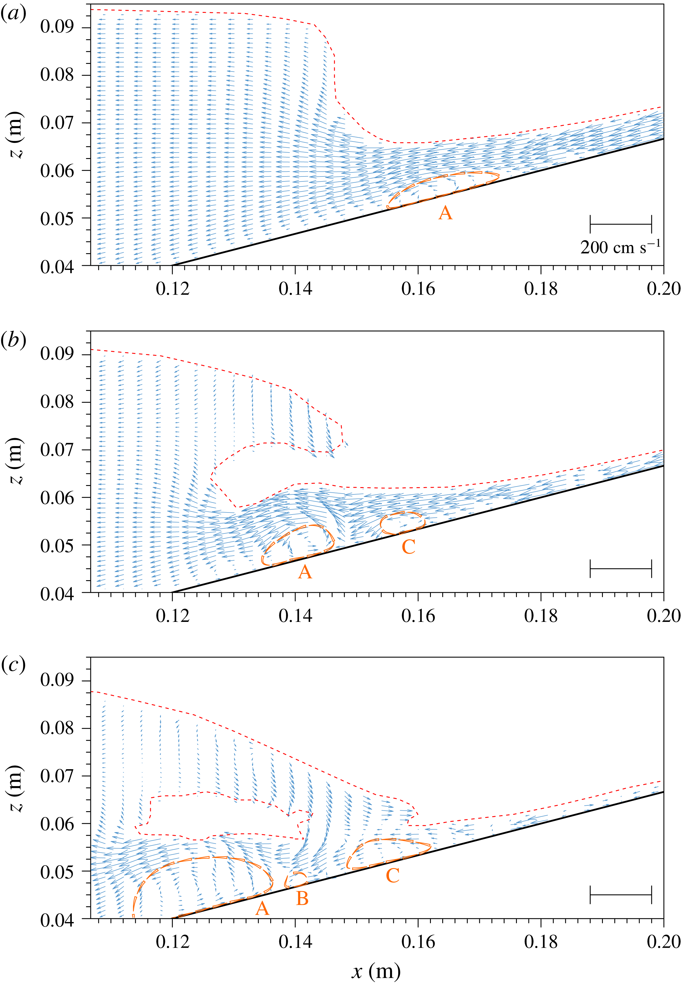
Figure 9. Measured velocity fields for
 $11.75~\text{cm}<x<20~\text{cm}$
and
$11.75~\text{cm}<x<20~\text{cm}$
and
 $1.011~\text{s}<t<1.111~\text{s}$
, during the rundown phase. A hydraulic jump occurred at
$1.011~\text{s}<t<1.111~\text{s}$
, during the rundown phase. A hydraulic jump occurred at
 $t=1.011~\text{s}$
. Experimental data have been downsampled to 3.25 and 10 arrows
$t=1.011~\text{s}$
. Experimental data have been downsampled to 3.25 and 10 arrows
 $\text{cm}^{-1}$
in the horizontal and vertical directions, respectively. Vortices are marked with triangles, indicating the direction of rotation, and tagged with letters. (a)
$\text{cm}^{-1}$
in the horizontal and vertical directions, respectively. Vortices are marked with triangles, indicating the direction of rotation, and tagged with letters. (a)
 $t=1.011~\text{s}$
, (b)
$t=1.011~\text{s}$
, (b)
 $t=1.075~\text{s}$
and (c)
$t=1.075~\text{s}$
and (c)
 $t=1.111~\text{s}$
.
$t=1.111~\text{s}$
.
In figure 9 several snapshots of free-surface profiles and velocity fields for
 $1.011~\text{s}<t<1.111~\text{s}$
are presented. A hydraulic jump with a nearly vertical free surface occurred at
$1.011~\text{s}<t<1.111~\text{s}$
are presented. A hydraulic jump with a nearly vertical free surface occurred at
 $t=$
1.011 s. The free surface eventually curled over towards the shore (as shown by the profiles at
$t=$
1.011 s. The free surface eventually curled over towards the shore (as shown by the profiles at
 $t=1.075~\text{s}$
in figure 9) and impinged on the fast incoming rundown flow (at
$t=1.075~\text{s}$
in figure 9) and impinged on the fast incoming rundown flow (at
 $t=1.111~\text{s}$
). A well-organized vortex structure (A) was first observed on the shoreward side of the hydraulic jump,
$t=1.111~\text{s}$
). A well-organized vortex structure (A) was first observed on the shoreward side of the hydraulic jump,
 $15.5~\text{cm}<x<17.5~\text{cm}$
(see
$15.5~\text{cm}<x<17.5~\text{cm}$
(see
 $t=1.011~\text{s}$
in figure 9). The vortex rotated in the counter-clockwise direction and was advected by the rundown flow in the offshore direction. Additional vortices (B and C) were generated as the impinging jet reached the water surface.
$t=1.011~\text{s}$
in figure 9). The vortex rotated in the counter-clockwise direction and was advected by the rundown flow in the offshore direction. Additional vortices (B and C) were generated as the impinging jet reached the water surface.

Figure 10. Flow visualization snapshot from the experiments for FOV S2 at
 $t=1.01~\text{s}$
.
$t=1.01~\text{s}$
.
 $X$
–
$X$
–
 $Z$
reference frame. Vortices are marked with triangles, indicating the direction of rotation, and tagged with letters.
$Z$
reference frame. Vortices are marked with triangles, indicating the direction of rotation, and tagged with letters.
Figure 10 shows a flow visualization snapshot from the experiments for FOV S2 at
 $t=1.01~\text{s}$
. This picture corresponds to (almost) the same instant and to a zoom-in region of figure 9(a), therefore it provides higher resolution. The free surface can be distinguished as a brighter line, as explained before. The figure shows the main vortex (A, anti-clockwise) induced by the fast rundown flow in the vicinity of the hydraulic jump, with dimensions approximately 1.2 cm long and 4 mm high, centred at
$t=1.01~\text{s}$
. This picture corresponds to (almost) the same instant and to a zoom-in region of figure 9(a), therefore it provides higher resolution. The free surface can be distinguished as a brighter line, as explained before. The figure shows the main vortex (A, anti-clockwise) induced by the fast rundown flow in the vicinity of the hydraulic jump, with dimensions approximately 1.2 cm long and 4 mm high, centred at
 $X=17.05~\text{cm}$
and
$X=17.05~\text{cm}$
and
 $Z=0.25~\text{cm}$
. Since the local water depth in the
$Z=0.25~\text{cm}$
. Since the local water depth in the
 $Z$
direction at
$Z$
direction at
 $X=17.05~\text{cm}$
is 1.2 cm, this flow feature represents an obstruction to the flow of approximately one-third of the water depth. A quiescent area can be found upstream (
$X=17.05~\text{cm}$
is 1.2 cm, this flow feature represents an obstruction to the flow of approximately one-third of the water depth. A quiescent area can be found upstream (
 $X>18~\text{cm}$
,
$X>18~\text{cm}$
,
 $Z<1~\text{mm}$
), causing a smooth transition between the flow reversal point at the slope surface (outside the view presented) and the flow above the main vortex. In the transition between both areas, a smaller clockwise vortex (B) appears (
$Z<1~\text{mm}$
), causing a smooth transition between the flow reversal point at the slope surface (outside the view presented) and the flow above the main vortex. In the transition between both areas, a smaller clockwise vortex (B) appears (
 $X=17.85~\text{cm}$
).
$X=17.85~\text{cm}$
).
3 Numerical modelling
In this section we introduce the numerical model and its limitations. Afterwards, we describe the set-up of the simulation, including the computational mesh, and boundary and initial conditions. Finally, we check the numerical results with experimental observations.
3.1 Numerical model governing equations
The numerical model (https://github.com/phicau/olaFlow) employed in this paper is a modification of the open source code OpenFOAM® (Weller et al. Reference Weller, Tabor, Jasak and Fureby1998). The modifications have been previously checked against experimental data and other existing numerical results (Higuera, Lara & Losada Reference Higuera, Lara and Losada2013a ,Reference Higuera, Lara and Losada b , Reference Higuera, Lara and Losada2014). For completeness, some of the essential elements of the numerical model are summarized next.
This numerical model solves the 3D Reynolds-averaged Navier–Stokes (RANS) equations for two incompressible phases (water and air). The free surface between water and air is captured with the volume of fluid (VOF) technique (Hirt & Nichols Reference Hirt and Nichols1981).
The RANS equations adopted by the model are expressed as
 $$\begin{eqnarray}\displaystyle & \displaystyle \unicode[STIX]{x1D735}\boldsymbol{\cdot }(\unicode[STIX]{x1D70C}\,\boldsymbol{U})=0, & \displaystyle\end{eqnarray}$$
 $$\begin{eqnarray}\displaystyle & \displaystyle \frac{\unicode[STIX]{x2202}\unicode[STIX]{x1D70C}\boldsymbol{U}}{\unicode[STIX]{x2202}t}+\unicode[STIX]{x1D735}\boldsymbol{\cdot }(\unicode[STIX]{x1D70C}\boldsymbol{U}\boldsymbol{U})=-\unicode[STIX]{x1D735}p^{\ast }-\boldsymbol{g}\boldsymbol{\cdot }\boldsymbol{r}\,\unicode[STIX]{x1D735}\unicode[STIX]{x1D70C}+\unicode[STIX]{x1D735}\boldsymbol{\cdot }(\unicode[STIX]{x1D707}\unicode[STIX]{x1D735}\boldsymbol{U}-\unicode[STIX]{x1D70C}\overline{\boldsymbol{U}^{\prime }\boldsymbol{U}^{\prime }})+\unicode[STIX]{x1D70E}\unicode[STIX]{x1D705}\unicode[STIX]{x1D735}\unicode[STIX]{x1D6FC}, & \displaystyle\end{eqnarray}$$
in which
 $\unicode[STIX]{x1D70C}$
is the fluid density,
$\unicode[STIX]{x1D70C}$
is the fluid density,
 $\boldsymbol{U}$
is the Reynolds-averaged velocity vector, and
$\boldsymbol{U}$
is the Reynolds-averaged velocity vector, and
 $\unicode[STIX]{x1D735}$
is the gradient vector
$\unicode[STIX]{x1D735}$
is the gradient vector
 $(\unicode[STIX]{x2202}/\unicode[STIX]{x2202}x,\unicode[STIX]{x2202}/\unicode[STIX]{x2202}y,\unicode[STIX]{x2202}/\unicode[STIX]{x2202}z)$
. Time is denoted by
$(\unicode[STIX]{x2202}/\unicode[STIX]{x2202}x,\unicode[STIX]{x2202}/\unicode[STIX]{x2202}y,\unicode[STIX]{x2202}/\unicode[STIX]{x2202}z)$
. Time is denoted by
 $t$
,
$t$
,
 $p^{\ast }=p-\unicode[STIX]{x1D70C}\,\boldsymbol{g}\boldsymbol{\cdot }\boldsymbol{r}$
is the dynamic pressure, and
$p^{\ast }=p-\unicode[STIX]{x1D70C}\,\boldsymbol{g}\boldsymbol{\cdot }\boldsymbol{r}$
is the dynamic pressure, and
 $p$
is the total pressure;
$p$
is the total pressure;
 $\boldsymbol{g}$
is the acceleration due to gravity and
$\boldsymbol{g}$
is the acceleration due to gravity and
 $\boldsymbol{r}$
is the position vector.
$\boldsymbol{r}$
is the position vector.
In the viscous term in (3.2),
 $\unicode[STIX]{x1D707}$
represents the molecular dynamic viscosity of the fluid, and
$\unicode[STIX]{x1D707}$
represents the molecular dynamic viscosity of the fluid, and
 $\unicode[STIX]{x1D70C}\overline{\boldsymbol{U}^{\prime }\boldsymbol{U}^{\prime }}$
denotes the Reynolds stresses, with the overbar denoting the ensemble average. Using the gradient hypothesis, the Reynolds stress can be modelled as a gradient of the averaged velocity with a dynamic turbulent viscosity (
$\unicode[STIX]{x1D70C}\overline{\boldsymbol{U}^{\prime }\boldsymbol{U}^{\prime }}$
denotes the Reynolds stresses, with the overbar denoting the ensemble average. Using the gradient hypothesis, the Reynolds stress can be modelled as a gradient of the averaged velocity with a dynamic turbulent viscosity (
 $\unicode[STIX]{x1D707}_{t}$
), which is modelled by different turbulence closure models. Finally, the viscous term can be written as
$\unicode[STIX]{x1D707}_{t}$
), which is modelled by different turbulence closure models. Finally, the viscous term can be written as
 $\unicode[STIX]{x1D735}\boldsymbol{\cdot }(\unicode[STIX]{x1D707}_{eff}\unicode[STIX]{x1D735}\boldsymbol{U})$
with the effective dynamic viscosity
$\unicode[STIX]{x1D735}\boldsymbol{\cdot }(\unicode[STIX]{x1D707}_{eff}\unicode[STIX]{x1D735}\boldsymbol{U})$
with the effective dynamic viscosity
 $\unicode[STIX]{x1D707}_{eff}$
, comprising the molecular and turbulent components.
$\unicode[STIX]{x1D707}_{eff}$
, comprising the molecular and turbulent components.
The last term in (3.2) represents the surface tension force. The continuum surface force (CSF) method (Brackbill, Kothe & Zemach Reference Brackbill, Kothe and Zemach1992) transforms the actual surface force into a body force, which acts at the interface between fluids.
 $\unicode[STIX]{x1D70E}$
is the surface tension coefficient;
$\unicode[STIX]{x1D70E}$
is the surface tension coefficient;
 $\unicode[STIX]{x1D705}$
is the curvature of the free surface, being calculated as
$\unicode[STIX]{x1D705}$
is the curvature of the free surface, being calculated as
 $\unicode[STIX]{x1D735}\boldsymbol{\cdot }(\unicode[STIX]{x1D735}\unicode[STIX]{x1D6FC}/|\unicode[STIX]{x1D735}\unicode[STIX]{x1D6FC}|)$
, where the volume of fluid (VOF) indicator function
$\unicode[STIX]{x1D735}\boldsymbol{\cdot }(\unicode[STIX]{x1D735}\unicode[STIX]{x1D6FC}/|\unicode[STIX]{x1D735}\unicode[STIX]{x1D6FC}|)$
, where the volume of fluid (VOF) indicator function
 $\unicode[STIX]{x1D6FC}$
represents the amount of water per unit volume in a computational cell. Thus,
$\unicode[STIX]{x1D6FC}$
represents the amount of water per unit volume in a computational cell. Thus,
 $\unicode[STIX]{x1D6FC}=1$
marks a pure water cell,
$\unicode[STIX]{x1D6FC}=1$
marks a pure water cell,
 $\unicode[STIX]{x1D6FC}=0$
denotes a pure air cell, and
$\unicode[STIX]{x1D6FC}=0$
denotes a pure air cell, and
 $0<\unicode[STIX]{x1D6FC}<1$
represent the interfacial cells. In order to obtain a physically meaningful solution,
$0<\unicode[STIX]{x1D6FC}<1$
represent the interfacial cells. In order to obtain a physically meaningful solution,
 $\unicode[STIX]{x1D6FC}$
needs to be conservative, strictly bounded between 0 and 1, and maintain a sharp interface. Fluid properties such as density (
$\unicode[STIX]{x1D6FC}$
needs to be conservative, strictly bounded between 0 and 1, and maintain a sharp interface. Fluid properties such as density (
 $\unicode[STIX]{x1D70C}$
) and kinematic and dynamic viscosities (
$\unicode[STIX]{x1D70C}$
) and kinematic and dynamic viscosities (
 $\unicode[STIX]{x1D708}$
,
$\unicode[STIX]{x1D708}$
,
 $\unicode[STIX]{x1D707}$
) are calculated as a weighted average between water and air, e.g.
$\unicode[STIX]{x1D707}$
) are calculated as a weighted average between water and air, e.g.
 $$\begin{eqnarray}\displaystyle \unicode[STIX]{x1D70C}=\unicode[STIX]{x1D6FC}\,\unicode[STIX]{x1D70C}_{w}+(1-\unicode[STIX]{x1D6FC})\,\unicode[STIX]{x1D70C}_{a}, & & \displaystyle\end{eqnarray}$$
where subscripts
 $w$
and
$w$
and
 $a$
denote water and air, respectively.
$a$
denote water and air, respectively.
The evolution of the VOF (
 $\unicode[STIX]{x1D6FC}$
) is prescribed by a conservative advection equation derived from the conservation of mass expression (Hirt & Nichols Reference Hirt and Nichols1981). In this interface capturing method, the free surface is not explicitly reconstructed at any stage. Since numerical solutions of an advection equation typically suffer from diffusion, an artificial compression (i.e. anti-diffusion) term acting only at the interface (
$\unicode[STIX]{x1D6FC}$
) is prescribed by a conservative advection equation derived from the conservation of mass expression (Hirt & Nichols Reference Hirt and Nichols1981). In this interface capturing method, the free surface is not explicitly reconstructed at any stage. Since numerical solutions of an advection equation typically suffer from diffusion, an artificial compression (i.e. anti-diffusion) term acting only at the interface (
 $0<\unicode[STIX]{x1D6FC}<1$
), intended to prevent the excessive smearing of the fluid interface, is added (Berberovic et al.
Reference Berberovic, Hinsberg, van Jakirlic, Roisman and Tropea2009):
$0<\unicode[STIX]{x1D6FC}<1$
), intended to prevent the excessive smearing of the fluid interface, is added (Berberovic et al.
Reference Berberovic, Hinsberg, van Jakirlic, Roisman and Tropea2009):
 $$\begin{eqnarray}\displaystyle \frac{\unicode[STIX]{x2202}\unicode[STIX]{x1D6FC}}{\unicode[STIX]{x2202}t}+\unicode[STIX]{x1D735}\boldsymbol{\cdot }(\unicode[STIX]{x1D6FC}\boldsymbol{U})+\unicode[STIX]{x1D735}\boldsymbol{\cdot }[\unicode[STIX]{x1D6FC}(1-\unicode[STIX]{x1D6FC})\boldsymbol{U}_{c}]=0. & & \displaystyle\end{eqnarray}$$
Here,
 $\boldsymbol{U}_{c}$
is a compression velocity oriented in the normal direction to the interface
$\boldsymbol{U}_{c}$
is a compression velocity oriented in the normal direction to the interface
 $(\unicode[STIX]{x1D735}\unicode[STIX]{x1D6FC}/|\unicode[STIX]{x1D735}\unicode[STIX]{x1D6FC}|)$
. The magnitude of
$(\unicode[STIX]{x1D735}\unicode[STIX]{x1D6FC}/|\unicode[STIX]{x1D735}\unicode[STIX]{x1D6FC}|)$
. The magnitude of
 $\boldsymbol{U}_{c}$
is calculated as the minimum between
$\boldsymbol{U}_{c}$
is calculated as the minimum between
 $c_{\unicode[STIX]{x1D6FC}}|\boldsymbol{U}|$
and the maximum velocity magnitude throughout the domain, to avoid creating artificial high velocities. The factor
$c_{\unicode[STIX]{x1D6FC}}|\boldsymbol{U}|$
and the maximum velocity magnitude throughout the domain, to avoid creating artificial high velocities. The factor
 $c_{\unicode[STIX]{x1D6FC}}$
is a constant for compression enhancement, normally taking a value of 1 (Gopala & van Wachem Reference Gopala and van Wachem2008).
$c_{\unicode[STIX]{x1D6FC}}$
is a constant for compression enhancement, normally taking a value of 1 (Gopala & van Wachem Reference Gopala and van Wachem2008).
3.2 Numerical model limitations
Navier–Stokes equations provide substantial benefits due to their small number of underlying assumptions. Nevertheless, numerical models possess limitations inherent to the numerical methods implemented in them. There are several shortcomings of the numerical model used in this paper, concerning primarily with the VOF method and the surface tension force.
The VOF implementation in OpenFOAM® is an algebraic interface capturing method. Low computational cost and strict mass conservation are significant advantages of this method. However, the main disadvantages of the method are diffusivity and that the calculation of the curvature of the interface is not accurate.
The diffusivity of the advection equation causes the transition between phases (water and air) not to be perfectly sharp, as observed physically. After adopting the artificial compression term, equation (3.4), the numerically obtained interface is smeared only over a few cells. Algebraic interface capturing methods are also known to generate non-physical flows at the interface, called spurious velocities or parasitic currents (Deshpande, Anumolu & Trujillo Reference Deshpande, Anumolu and Trujillo2012). Francois et al. (Reference Francois, Cummins, Dendy, Kothe, Sicilian and Williams2006) identified the main causes as inaccuracies in the interface curvature calculation and a lack of a discrete force balance between the pressure gradient and surface tension. This means that parasitic currents derive both from the low-order VOF technique and the application of the CSF method (Brackbill et al. Reference Brackbill, Kothe and Zemach1992).
The effects of spurious velocities are not a major issue for inertia-dominated flows (Deshpande et al.
Reference Deshpande, Anumolu and Trujillo2012). Nevertheless, their magnitude increases at smaller scales (i.e. capillary flows) (Lafaurie et al.
Reference Lafaurie, Nardone, Scardovelli, Zaleski and Zanetti1994), because the capillary number (the capillary number is defined as
 $\unicode[STIX]{x1D707}U/\unicode[STIX]{x1D70E}$
, in which
$\unicode[STIX]{x1D707}U/\unicode[STIX]{x1D70E}$
, in which
 $U$
is a characteristic velocity,
$U$
is a characteristic velocity,
 $\unicode[STIX]{x1D707}$
is dynamic viscosity and
$\unicode[STIX]{x1D707}$
is dynamic viscosity and
 $\unicode[STIX]{x1D70E}$
is the surface tension coefficient), which measures the relative effect of viscous forces versus surface tension forces, decreases proportionally with the scale.
$\unicode[STIX]{x1D70E}$
is the surface tension coefficient), which measures the relative effect of viscous forces versus surface tension forces, decreases proportionally with the scale.
In view of these misgivings, the numerical model might have limited applicability to simulate flows in which the free surface presents a strong curvature or significant surface tension. In the present study, the quality of numerical results is guaranteed for the largest portion of the computational domain, since the effective wavelength of the solitary wave is close to 1 m, within the gravity-waves regime. Under these conditions, surface tension effects are four orders of magnitude smaller than gravity (Holthuijsen Reference Holthuijsen2010). There is only a small area in which surface tension dominates: the meniscus at the moving shoreline. The effects of parasitic currents in the simulation over this area are later analysed in figure 12. Fortunately, the meniscus effects appear to be extremely limited, as the region of influence is quite small when compared with the entire swash zone. Therefore, the numerical model is capable of capturing the details of bottom boundary layer velocity structure and the vortex generation during the runup and rundown phases.
Several numerical techniques that can remedy the numerical model limitations are discussed in § 5.
3.3 Numerical set-up of the case
3.3.1 Mesh
A 3D mesh, representing the physical wave flume described in § 2.1, has been created. The final mesh has been produced after several iterations and mesh sensitivity analyses. The aim is to obtain high resolution and high-quality results in the areas of interest, while minimizing the number of cells elsewhere to reduce the computational cost. When cell size gradation is introduced, it has been performed by means of a geometric progression. A side view of the final mesh is presented in figure 11.
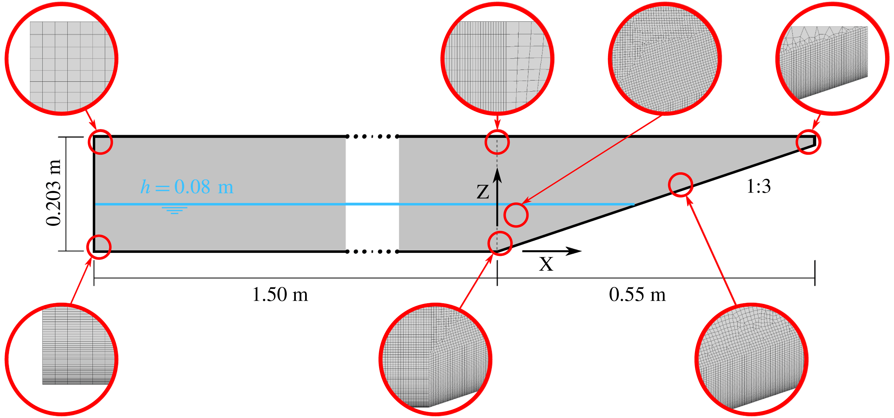
Figure 11. A sketch of the vertical plane view of the mesh used in the numerical model. Each circle provides a zoom-in view of the actual cells.

Figure 12. Evolution of the time derivative of free-surface elevation in space and time. Units in
 $\text{m}~\text{s}^{-1}$
.
$\text{m}~\text{s}^{-1}$
.
Special emphasis has been put in obtaining a high-quality characterization of the flow within the bottom boundary layer (BL), where flow separation and vortex generation take place (see figure 7). Although the BL thickness changes throughout the swash flow process, it can be roughly estimated using the Blasius boundary layer solution (Schlichting Reference Schlichting1979). For the present wave conditions, the BL thickness can be estimated as 4.5 mm–
 $6.5~\text{mm}$
(laminar solution). Thus, a structured grid extending 20 mm in the vertical direction has been created in the BL area, adjacent to the bottom. In the BL, the vertical gradients are expected to be larger than the horizontal gradients. Hence, the vertical resolution of cells at the bottom has been enhanced to 0.1 mm, higher than the one that the PIV experiments provided for the most detailed field of view. The vertical cell size increases up to 1 mm, 20 mm away from the bottom. The cells in the BL over the slope are aligned with the sloping bottom and with the vertical direction (
$6.5~\text{mm}$
(laminar solution). Thus, a structured grid extending 20 mm in the vertical direction has been created in the BL area, adjacent to the bottom. In the BL, the vertical gradients are expected to be larger than the horizontal gradients. Hence, the vertical resolution of cells at the bottom has been enhanced to 0.1 mm, higher than the one that the PIV experiments provided for the most detailed field of view. The vertical cell size increases up to 1 mm, 20 mm away from the bottom. The cells in the BL over the slope are aligned with the sloping bottom and with the vertical direction (
 $z$
-axis); thereby, a slight non-orthogonality exists among the centre-to-centre line of adjacent cells and the normal vector to the face that they share. In OpenFOAM® the non-orthogonality error is corrected by means of the over-relaxed approach (Jasak Reference Jasak1996) to preserve second-order accuracy in space.
$z$
-axis); thereby, a slight non-orthogonality exists among the centre-to-centre line of adjacent cells and the normal vector to the face that they share. In OpenFOAM® the non-orthogonality error is corrected by means of the over-relaxed approach (Jasak Reference Jasak1996) to preserve second-order accuracy in space.
The wave generation and propagation region (i.e. constant-water-depth area) is 1.5 m long and 0.203 m high, much shorter than that in the actual wave flume, but its length does not impact the wave shape (i.e. the wave is free of influences from the wave generation boundary). The mesh in the constant-water-depth region is structured and cells are orthogonal. Cell size gradation in both vertical and horizontal directions has been introduced. In the longitudinal direction, cells are 5 mm long at the wave generation boundary, decreasing to 1 mm towards the toe of the slope. In the vertical direction, cells outside the BL are 1 mm high below the still-water level (
 $z=0.08~\text{m}$
). At this resolution the wave height (2.9 cm) is discretized by 29 cells, which is enough to obtain excellent detail. Finally, cell height grows to 5 mm at the top boundary.
$z=0.08~\text{m}$
). At this resolution the wave height (2.9 cm) is discretized by 29 cells, which is enough to obtain excellent detail. Finally, cell height grows to 5 mm at the top boundary.
The flow region above the slope constitutes the area of primary interest. This zone spans 0.55 m horizontally and 0.203 m vertically, and includes a sloping bottom (1 : 3). The horizontal discretization is kept constant and equal to 1 mm throughout the area. Above the BL, the mesh is non-structured and the vertical cell size increases from 1 mm to 5 mm, matching that in the constant-water-depth region (see figure 11). Since VOF advection is known to produce less diffusion for hexahedral cells (Deshpande et al. Reference Deshpande, Anumolu and Trujillo2012), the meshing procedure produces a majority of this type of cells versus triangular prisms.
The 3D mesh has been created by lateral extrusion (
 $y$
-direction) of the mesh shown in figure 11, over half of the experimental flume width (125 mm). Each of the 63 slices has a constant width close to 2 mm. The 3D mesh is formed predominantly by quadrilateral prisms (hexahedra), totalling 8.8 million cells. The simulation of the 4.5 s laboratory experiment takes 169 h in 24 cores of an Intel Xeon (2.50 GHz) workstation.
$y$
-direction) of the mesh shown in figure 11, over half of the experimental flume width (125 mm). Each of the 63 slices has a constant width close to 2 mm. The 3D mesh is formed predominantly by quadrilateral prisms (hexahedra), totalling 8.8 million cells. The simulation of the 4.5 s laboratory experiment takes 169 h in 24 cores of an Intel Xeon (2.50 GHz) workstation.
A 2D mesh (single slice) was also tested. No noticeable differences in free-surface elevation and velocity were found before the onset of wave breaking, when fully 3D flow patterns develop. However, the 3D simulation shows a much higher degree of energy dissipation after wave breaking, with the 2D simulation presenting more agitation (i.e. larger velocities).
3.3.2 Initial and boundary conditions
The solitary wave is generated at the left boundary, using an updated version of the wave generation module presented in Higuera et al. (Reference Higuera, Lara and Losada2013a
). The target solitary wave velocity and height profiles have been calculated according to the third-order solution in Grimshaw (Reference Grimshaw1971). The solitary wave is simulated so that the targeted wave height is
 $H_{0}=2.9~\text{cm}$
in the water depth of
$H_{0}=2.9~\text{cm}$
in the water depth of
 $h_{0}=8.0~\text{cm}$
, resulting in a wave nonlinearity of
$h_{0}=8.0~\text{cm}$
, resulting in a wave nonlinearity of
 $H_{0}/h_{0}=0.3625$
. The numerical active wave absorption (Higuera et al.
Reference Higuera, Lara and Losada2013a
) is activated; therefore, any reflections from the slope are absorbed at the numerical wavemaker.
$H_{0}/h_{0}=0.3625$
. The numerical active wave absorption (Higuera et al.
Reference Higuera, Lara and Losada2013a
) is activated; therefore, any reflections from the slope are absorbed at the numerical wavemaker.
On the bottom boundary of the flume, the no-slip boundary condition is applied. Since only half of the flume is discretized in the spanwise (
 $y$
) direction, a symmetry boundary condition has been set on the centreline boundary and a free-slip condition has been set on the sidewall boundary, because resolving the boundary layer on the lateral wall is out of the scope of this paper.
$y$
) direction, a symmetry boundary condition has been set on the centreline boundary and a free-slip condition has been set on the sidewall boundary, because resolving the boundary layer on the lateral wall is out of the scope of this paper.
The swash flow is wave-driven and laminar during the runup phase. During rundown, the flow becomes gravity-driven and overcomes the laminar regime, exceeding the 500 Reynolds number limit defined for open channel flow. Therefore, the simulation has been run with the
 $k{-}\unicode[STIX]{x1D714}$
SST turbulence model presented in Devolder, Rauwoens & Troch (Reference Devolder, Rauwoens and Troch2017). This recent version is validated and includes a buoyancy term in the turbulent kinetic energy equation that manages adequately the turbulence level at the free surface. A comparison between the present simulation and an analogous one assuming laminar flow (i.e. disregarding Reynolds stress modelling) is presented in § C of the supplementary material available at https://doi.org/10.1017/
jfm.2018.321.
$k{-}\unicode[STIX]{x1D714}$
SST turbulence model presented in Devolder, Rauwoens & Troch (Reference Devolder, Rauwoens and Troch2017). This recent version is validated and includes a buoyancy term in the turbulent kinetic energy equation that manages adequately the turbulence level at the free surface. A comparison between the present simulation and an analogous one assuming laminar flow (i.e. disregarding Reynolds stress modelling) is presented in § C of the supplementary material available at https://doi.org/10.1017/
jfm.2018.321.
The boundary conditions for turbulence variables (
 $k$
and
$k$
and
 $\unicode[STIX]{x1D714}$
) provide wall function approximations for both low- and high-Reynolds-number turbulence models. Initial values for
$\unicode[STIX]{x1D714}$
) provide wall function approximations for both low- and high-Reynolds-number turbulence models. Initial values for
 $k$
and
$k$
and
 $\unicode[STIX]{x1D714}$
are very small but not zero, to avoid singularities when solving the turbulence equations. Moreover, as the case starts from rest, the resulting initial kinematic turbulent viscosity (
$\unicode[STIX]{x1D714}$
are very small but not zero, to avoid singularities when solving the turbulence equations. Moreover, as the case starts from rest, the resulting initial kinematic turbulent viscosity (
 $\unicode[STIX]{x1D708}_{t}$
) for the chosen values is several orders of magnitude smaller than the molecular kinematic viscosity of water.
$\unicode[STIX]{x1D708}_{t}$
) for the chosen values is several orders of magnitude smaller than the molecular kinematic viscosity of water.
Because of the presence of a contact point (water–air–solid) at the shoreline, a meniscus develops in the water phase. Since the contact angle between water and acrylic (polymethyl methacrylate) is
 $73^{\circ }$
(Omenyi, Smith & Neumann Reference Omenyi, Smith and Neumann1980), the contact angle boundary condition applies the fixed zero gradient to the VOF function
$73^{\circ }$
(Omenyi, Smith & Neumann Reference Omenyi, Smith and Neumann1980), the contact angle boundary condition applies the fixed zero gradient to the VOF function
 $\unicode[STIX]{x1D6FC}$
in this direction.
$\unicode[STIX]{x1D6FC}$
in this direction.
Initially the free surface is positioned at
 $z=8.0~\text{cm}$
, which differs slightly from the equilibrium state position because of the meniscus at the shoreline. This difference would generate small but noticeable waves (height approximately 1.5 mm, 5 % of the solitary wave height) as the meniscus develops. These oscillations are dampened during a precursor simulation in which the static equilibrium (zero velocity and fully developed meniscus) is established. Afterwards, the simulation is restarted and the solitary wave is generated.
$z=8.0~\text{cm}$
, which differs slightly from the equilibrium state position because of the meniscus at the shoreline. This difference would generate small but noticeable waves (height approximately 1.5 mm, 5 % of the solitary wave height) as the meniscus develops. These oscillations are dampened during a precursor simulation in which the static equilibrium (zero velocity and fully developed meniscus) is established. Afterwards, the simulation is restarted and the solitary wave is generated.
3.4 Comparisons between numerical results and experimental observations
In this section, we first compare the numerical and experimental results through the detailed study of free-surface elevation profiles and velocity fields. Additional physical quantities, such as bottom shear stress and pressure gradients, will be discussed in the next section.
The numerical data presented in the following sections have been averaged over the spanwise direction, unless stated otherwise. Any spanwise variability observed is induced by 3D flow features, which are virtually non-existent before wave breaking. Nevertheless, the spanwise averaging helps to obtain more consistent velocity profiles near the shoreline, where spurious velocities introduce random local variability.
The time reference system of the numerical simulations matches that of the laboratory experiments. The zero time (
 $t=0~\text{s}$
) has been set when the crest of the solitary wave is at the toe of the slope (
$t=0~\text{s}$
) has been set when the crest of the solitary wave is at the toe of the slope (
 $x=0~\text{m}$
).
$x=0~\text{m}$
).
3.4.1 Free-surface elevation and runup
One of the advantages of numerical simulations is the capability to produce high-resolution solutions in space and time. An example is shown in figure 12 for the evolution of free-surface elevations temporarily and spatially. The free surface has been calculated as the isosurface of
 $\unicode[STIX]{x1D6FC}=0.5$
.
$\unicode[STIX]{x1D6FC}=0.5$
.
In figure 12 the horizontal axis is time and the vertical axis is distance covering the full length of the numerical wave flume. The wave generation boundary is located at
 $x=-1.50~\text{m}$
, while the initial still-water shoreline is located at
$x=-1.50~\text{m}$
, while the initial still-water shoreline is located at
 $x=0.234~\text{m}$
. The colour bar indicates the time derivative of free-surface elevation. The positive values represent the acceleration phase (or upward free-surface velocity), while the negative values represent the deceleration phase (downward free-surface velocity). Thus, individual waves can be identified by a light-to-dark colour transition.
$x=0.234~\text{m}$
. The colour bar indicates the time derivative of free-surface elevation. The positive values represent the acceleration phase (or upward free-surface velocity), while the negative values represent the deceleration phase (downward free-surface velocity). Thus, individual waves can be identified by a light-to-dark colour transition.
The incoming wave becomes noticeable at approximately
 $t=-1.80~\text{s}$
. As the main solitary wave reaches its stable profile, small trailing waves, which have smaller amplitudes and are of the same magnitude as those measured in the experiments, are also visible. The trailing waves have smaller celerity than the solitary wave, resulting in clear separation.
$t=-1.80~\text{s}$
. As the main solitary wave reaches its stable profile, small trailing waves, which have smaller amplitudes and are of the same magnitude as those measured in the experiments, are also visible. The trailing waves have smaller celerity than the solitary wave, resulting in clear separation.
A meniscus exists at the shoreline. On closer inspection over that area, parasitic currents appear in the air phase adjacent to the free surface. Despite being non-physical, the spurious velocities do not have significant impact on the overall numerical solution, since the shoreline is completely static and the meniscus is in equilibrium before the solitary wave reaches the shoreline (
 $t<-0.5~\text{s}$
). However, these velocities cause minor high-frequency oscillations locally, which produce extremely small waves (
$t<-0.5~\text{s}$
). However, these velocities cause minor high-frequency oscillations locally, which produce extremely small waves (
 ${<}1~\text{mm}$
, sub-cell scale) propagating offshore, and are barely noticeable in figure 12.
${<}1~\text{mm}$
, sub-cell scale) propagating offshore, and are barely noticeable in figure 12.
The evolution of free-surface elevation during runup and rundown phases will be studied later in greater detail. After the maximum runup height is reached the swash flow enters the rundown phase and becomes gravity-driven. During the final period of the rundown phase (
 $t>1~\text{s}$
), the noisy area at the top right corner (shoreline area) is the result of the transformation of the supercritical rundown flow into the subcritical water body, through a hydraulic jump.
$t>1~\text{s}$
), the noisy area at the top right corner (shoreline area) is the result of the transformation of the supercritical rundown flow into the subcritical water body, through a hydraulic jump.
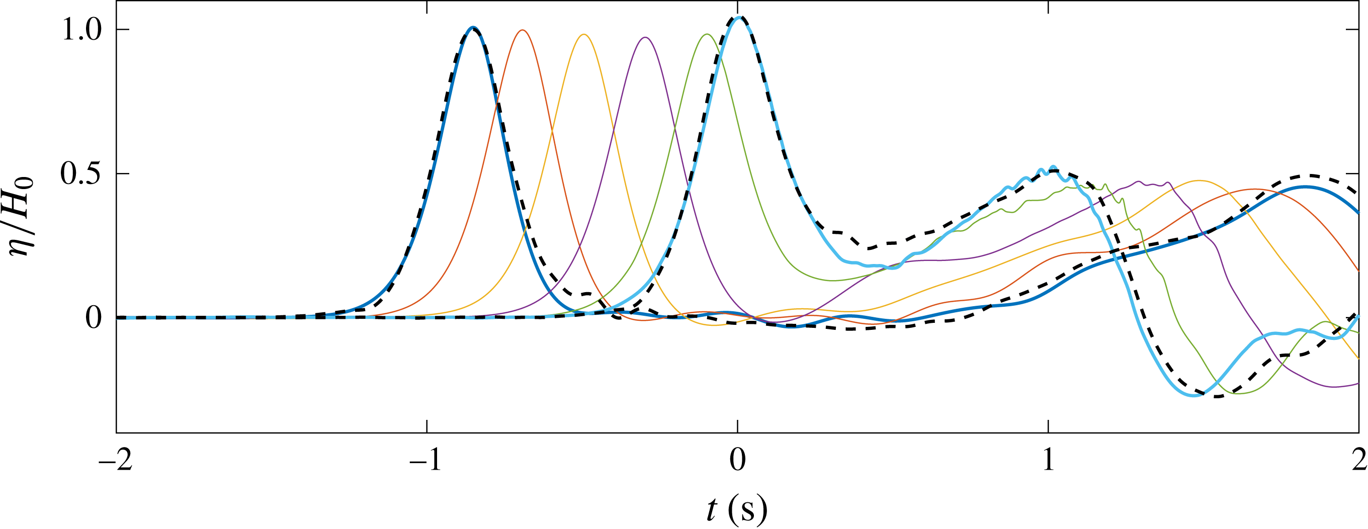
Figure 13. Numerical solutions for the time series of free-surface elevation in the constant-depth region. Experimental (dashed lines) and numerical (continuous lines) are compared at
 $x=-0.86~\text{m}$
and
$x=-0.86~\text{m}$
and
 $x=0.0~\text{m}$
. Additional numerical samplings took place along
$x=0.0~\text{m}$
. Additional numerical samplings took place along
 $y=0.061~\text{m}$
(centreline of the numerical wave flume) and
$y=0.061~\text{m}$
(centreline of the numerical wave flume) and
 $-0.70~\text{m}<x<-0.10~\text{m}$
with a 20 cm increment.
$-0.70~\text{m}<x<-0.10~\text{m}$
with a 20 cm increment.
The time histories of free-surface elevations at six locations in the constant-water-depth region are shown in figure 13. Since all the locations are far away from the wave generation boundary, no spurious boundary effects remain. The wave profiles present a consistent shape, although wave heights decrease slightly due to frictional dissipation in the bottom boundary layer. The wave dissipation rate has been studied separately for a solitary wave propagating on constant depth. The results are included in the supplementary material (§ A). Shoaling can also be noticed in the last two numerically obtained curves, when the wave approaches the slope.
Since the constant-depth region in the numerical domain has been shortened to 1.5 m, the first wave gauge location in the laboratory experiments that can be used for comparison is at
 $x=-0.86~\text{m}$
. The degree of accordance between the numerical and experimental time series of free-surface elevation is very good, with a relative wave height error of 0.7 %. Minor differences in wave shape appear in the leading edge, with a maximum deficit in elevation of approximately 2 % in the numerical results. Differences are more apparent in the trailing oscillations, which are significantly larger in the experiment.
$x=-0.86~\text{m}$
. The degree of accordance between the numerical and experimental time series of free-surface elevation is very good, with a relative wave height error of 0.7 %. Minor differences in wave shape appear in the leading edge, with a maximum deficit in elevation of approximately 2 % in the numerical results. Differences are more apparent in the trailing oscillations, which are significantly larger in the experiment.
The second experimental sampling location is at
 $x=0.0~\text{m}$
(toe of the slope). The wave height obtained from the numerical simulation agrees with the experimental data very well (0.4 % relative error). Globally, the shape of the numerically simulated wave is also in good agreement with experimental data. However, large discrepancies arise around
$x=0.0~\text{m}$
(toe of the slope). The wave height obtained from the numerical simulation agrees with the experimental data very well (0.4 % relative error). Globally, the shape of the numerically simulated wave is also in good agreement with experimental data. However, large discrepancies arise around
 $t=0.27~\text{s}$
, when the incident wave starts to interact with the reflected wave from the slope. The maximum relative error is less than 10 %. We remark that the reflected wave height is captured accurately by the numerical model.
$t=0.27~\text{s}$
, when the incident wave starts to interact with the reflected wave from the slope. The maximum relative error is less than 10 %. We remark that the reflected wave height is captured accurately by the numerical model.
The wave celerity can be estimated by tracking the locations of the wave crest. The estimated result is
 $1.01~\text{m}~\text{s}^{-1}$
, which is 1.9 % smaller than the theoretical value (
$1.01~\text{m}~\text{s}^{-1}$
, which is 1.9 % smaller than the theoretical value (
 $c=\sqrt{g\,(h_{0}+H_{0})}=1.03~\text{m}~\text{s}^{-1}$
, for the target wave height of
$c=\sqrt{g\,(h_{0}+H_{0})}=1.03~\text{m}~\text{s}^{-1}$
, for the target wave height of
 $H_{0}=2.9~\text{cm}$
).
$H_{0}=2.9~\text{cm}$
).
Figure 14. The experimental/numerical comparison of free-surface profiles during the runup and rundown phases. Numerical results are presented as individual markers, see legend for times. The experimental observations are represented as dashed lines. (a) Runup. (b) Rundown.
Snapshots of free-surface elevation profiles in the swash zone, obtained from numerical simulations and laboratory experiments, are plotted in figure 14. Figure 14(a) shows the surface profiles during the runup phase, while figure 14(b) is for the rundown phase.
During the initial phases of the runup process (
 $t=-0.14~\text{s}$
and 0.06 s) the largest discrepancy of 4 mm occurs close to the leftmost border. This effect is caused by the slightly different shape between the numerical and experimental solitary wave elevation profiles, which has also been commented upon in figure 13. The data/model agreement of the next three free-surface profiles is excellent, especially away from the moving shoreline. This comparison gives strong evidence on the numerical model limitations in accurately simulating the physics in the neighbourhood of the shoreline.
$t=-0.14~\text{s}$
and 0.06 s) the largest discrepancy of 4 mm occurs close to the leftmost border. This effect is caused by the slightly different shape between the numerical and experimental solitary wave elevation profiles, which has also been commented upon in figure 13. The data/model agreement of the next three free-surface profiles is excellent, especially away from the moving shoreline. This comparison gives strong evidence on the numerical model limitations in accurately simulating the physics in the neighbourhood of the shoreline.
The beginning of the rundown phase (i.e. maximum runup) takes place at virtually the same instant in the numerical simulation and in the experiment, as noted in figure 3. The numerical curve matches well with the thickness of the experimental profile, however, the numerical shoreline is positioned 1.2 cm further down the slope. Such situation continues until
 $t=0.96~\text{s}$
. Apparently, during the period, the shoreline velocity observed in the laboratory is higher than the numerical solution. In the offshore area, discrepancies are larger and grow with time. By the time
$t=0.96~\text{s}$
. Apparently, during the period, the shoreline velocity observed in the laboratory is higher than the numerical solution. In the offshore area, discrepancies are larger and grow with time. By the time
 $t=0.96~\text{s}$
the experimentally observed shoreline position has caught up with that of the numerical solution. However, the numerically obtained free surface is significantly steeper. Wave breaking also occurs earlier in the numerical simulation, at
$t=0.96~\text{s}$
the experimentally observed shoreline position has caught up with that of the numerical solution. However, the numerically obtained free surface is significantly steeper. Wave breaking also occurs earlier in the numerical simulation, at
 $t=0.97~\text{s}$
, as compared to
$t=0.97~\text{s}$
, as compared to
 $t=1.007~\text{s}$
in the experiments (see the timeline shown in figure 3). During the breaking process, the hydraulic jump overturns towards the shore and traps a pocket of air. Based on this comparison, it appears that time and space lags exist between the numerical results and laboratory observations, especially during the rundown phase. This could be caused by error accumulation due to the inaccurate modelling of the shoreline dynamics in the numerical model. More detailed discussions will be provided in the next section.
$t=1.007~\text{s}$
in the experiments (see the timeline shown in figure 3). During the breaking process, the hydraulic jump overturns towards the shore and traps a pocket of air. Based on this comparison, it appears that time and space lags exist between the numerical results and laboratory observations, especially during the rundown phase. This could be caused by error accumulation due to the inaccurate modelling of the shoreline dynamics in the numerical model. More detailed discussions will be provided in the next section.
Figure 15. Comparison of runup height. The numerical runup height is determined as the spanwise-averaged VOF level of
 $\unicode[STIX]{x1D6FC}=0.5$
contour line on the slope. Minimum and maximum bounds also plotted as dots to reflect the spanwise variability. Experimental points are depicted as crosses.
$\unicode[STIX]{x1D6FC}=0.5$
contour line on the slope. Minimum and maximum bounds also plotted as dots to reflect the spanwise variability. Experimental points are depicted as crosses.
The time series of runup height is presented in figure 15. Since the numerical simulation is three-dimensional, a small variability in water elevation exists in the spanwise direction (
 $y$
-axis). Therefore, numerically simulated runup height (continuous line) is calculated as the spanwise-averaged height of the shoreline, defined as the
$y$
-axis). Therefore, numerically simulated runup height (continuous line) is calculated as the spanwise-averaged height of the shoreline, defined as the
 $\unicode[STIX]{x1D6FC}=0.5$
contour line on the slope. Smaller isovalues, such as 0.1, yield virtually the same results because of the small cell size. The maxima and minima of the runup height in the spanwise direction from the numerical results are also plotted in the same figure. The differences among the averaged values and maximum/minimum values are negligible until wave breaking occurs. Experimental runup height measurements were obtained at certain instants only, including those from the profiles in figure 14, and are depicted as blue crosses.
$\unicode[STIX]{x1D6FC}=0.5$
contour line on the slope. Smaller isovalues, such as 0.1, yield virtually the same results because of the small cell size. The maxima and minima of the runup height in the spanwise direction from the numerical results are also plotted in the same figure. The differences among the averaged values and maximum/minimum values are negligible until wave breaking occurs. Experimental runup height measurements were obtained at certain instants only, including those from the profiles in figure 14, and are depicted as blue crosses.
Generally speaking, the agreement is very reasonable for the runup phase, although differences start to arise at the last stage of this phase. The maximum runup height observed in the laboratory is 8.4 cm, which is 4 mm (4.5 %) higher than the value obtained from the numerical model (7.96 cm,
 $R/H=2.745$
). Despite the discrepancy in magnitude, the instant at which maximum runup occurs is practically the same in the simulation and the laboratory experiment (0.004 s difference). Major discrepancies are found during rundown phase. The retreating velocity and acceleration of the shoreline are significantly larger in the laboratory experiment. This results in an important deviation at
$R/H=2.745$
). Despite the discrepancy in magnitude, the instant at which maximum runup occurs is practically the same in the simulation and the laboratory experiment (0.004 s difference). Major discrepancies are found during rundown phase. The retreating velocity and acceleration of the shoreline are significantly larger in the laboratory experiment. This results in an important deviation at
 $t=1.15~\text{s}$
, when the numerical solution shows a runup value of 3.7 cm higher than the laboratory measurement.
$t=1.15~\text{s}$
, when the numerical solution shows a runup value of 3.7 cm higher than the laboratory measurement.

Figure 16. The free-surface profile and velocity field comparisons during the shoaling phase at
 $t=0.00~\text{s}$
(a), 0.09 s (b) and 0.18 s (c), respectively. Experimental data are plotted as crosses, numerical data as dots. Three set of subpanels are presented at each instant. Top: numerical solutions for velocity field and free-surface elevation along the flume. Middle: horizontal velocity profiles in the water column at several cross-sections. Bottom: horizontal velocity profiles in the boundary layer. The resolution of the PIV data is between 0.5 mm and 1 mm.
$t=0.00~\text{s}$
(a), 0.09 s (b) and 0.18 s (c), respectively. Experimental data are plotted as crosses, numerical data as dots. Three set of subpanels are presented at each instant. Top: numerical solutions for velocity field and free-surface elevation along the flume. Middle: horizontal velocity profiles in the water column at several cross-sections. Bottom: horizontal velocity profiles in the boundary layer. The resolution of the PIV data is between 0.5 mm and 1 mm.

Figure 17. The free-surface profile and velocity field comparisons during the runup phase at
 $t=0.36~\text{s}$
(a), 0.54 s (b) and 0.63 s (c), respectively. The free-stream velocities are decelerating during this period. Captions are the same as those defined in figure 16.
$t=0.36~\text{s}$
(a), 0.54 s (b) and 0.63 s (c), respectively. The free-stream velocities are decelerating during this period. Captions are the same as those defined in figure 16.
Using Synolakis’ (Reference Synolakis1987) runup theory for non-breaking solitary waves, which is based on the nonlinear shallow water equations, the maximum runup height for the present experimental condition is 11.0 cm, which is almost 50 % higher than the observed experimental data and numerically simulated result. We note that Synolakis’ theory ignores the bottom frictional effects, which dissipate energy and hence reduce the runup height. Liu & Cho (Reference Liu and Cho1994) included the viscous bottom boundary layer effects in their numerical runup model, using the boundary integral equation method. Their model estimates a maximum runup value of 9.0 cm for the 1:3 slope, which is still approximately 10 % above the value shown in this work. The discrepancy could be attributed to the fact that Liu & Cho (Reference Liu and Cho1994) model did not take into consideration the meniscus in the vicinity of the moving shoreline.
3.4.2 Velocity profiles in the swash flow
In this section, the velocity profiles in the water column, including those inside the bottom boundary layer, are shown at different phases of the swash process. Both numerically simulated solutions and the PIV data are plotted together for comparison. Figure 2 indicates the location of the FOVs where PIV data have been recorded. We remark here that the smaller the FOVs, the higher resolution they yield. FOVs L2, L3 and L4 have been combined into a single plot and the numerical velocities have been averaged in the spanwise direction.
To manage the length of this paper only a selected set of snapshots of velocity profiles are presented in figures 16, 17 and 19–21. The following format is used in presenting the results and comparisons. Each figure consists of model/data comparisons at two or three instants. For each instant three sets of subpanels are shown. The top subpanel shows a snapshot of the free-surface elevation (densely packed dots for the numerical solutions and crosses for the experimental data) and the numerically calculated velocity field. The short grey vertical lines along the bottom and top of the horizontal axes indicate the location of the transects where horizontal velocity profiles are compared in the sets of subpanels below. The lower two sets of subpanels present the velocity profile comparisons. The middle set shows the comparison of horizontal velocity in the water column at the identified transects. Experimental data are represented by crosses and the numerical solution by dots. The density of the points is the actual resolution of the available data in both cases. In the numerical results, data points coincide with cell centres and in the laboratory experiment data points represent the output points of the HSPIV data. The bottom set displays zoom-in velocity profiles inside the bottom boundary layer.
Figure 16 shows velocity comparisons at the instants when the wave crest is above the toe of the slope (
 $t=0~\text{s}$
) and during the rest of the shoaling phase (
$t=0~\text{s}$
) and during the rest of the shoaling phase (
 $-0.47~\text{s}<t<0.29~\text{s}$
). The degree of accordance of the free-surface elevation is remarkable at the three instants. The free-stream velocities are slightly overestimated by the numerical model initially. Overall, the comparisons for velocity profiles are also good. However, significant discrepancies in the vicinity of the shoreline (
$-0.47~\text{s}<t<0.29~\text{s}$
). The degree of accordance of the free-surface elevation is remarkable at the three instants. The free-stream velocities are slightly overestimated by the numerical model initially. Overall, the comparisons for velocity profiles are also good. However, significant discrepancies in the vicinity of the shoreline (
 $x=23.63~\text{cm}$
) can be detected initially. Recall that the numerical model has most severe shortcomings in accurately modelling the shoreline dynamics, where the effects of surface tension and meniscus dominate.
$x=23.63~\text{cm}$
) can be detected initially. Recall that the numerical model has most severe shortcomings in accurately modelling the shoreline dynamics, where the effects of surface tension and meniscus dominate.
It is known that a slight difference in the free-surface elevation can result in much larger difference in the velocity field. This can be understood as follows. Using the long-wave theory, the horizontal velocity can be approximately related to the free-surface elevation as
 $U=\sqrt{g/h_{0}}\,\unicode[STIX]{x1D702}$
. In the present laboratory experiments the amplification factor,
$U=\sqrt{g/h_{0}}\,\unicode[STIX]{x1D702}$
. In the present laboratory experiments the amplification factor,
 $\sqrt{g/h_{0}}$
, is approximately
$\sqrt{g/h_{0}}$
, is approximately
 $11~\text{s}^{-1}$
for
$11~\text{s}^{-1}$
for
 $h_{0}=8~\text{cm}$
. In other words, if the free-surface elevation difference is 1 mm, the resulting difference in velocity is approximately
$h_{0}=8~\text{cm}$
. In other words, if the free-surface elevation difference is 1 mm, the resulting difference in velocity is approximately
 $1.1~\text{cm}~\text{s}^{-1}$
. This value must be regarded as the lower bound for error, since
$1.1~\text{cm}~\text{s}^{-1}$
. This value must be regarded as the lower bound for error, since
 $h$
decreases and
$h$
decreases and
 $\unicode[STIX]{x1D702}$
increases on the slope because of shoaling. At time
$\unicode[STIX]{x1D702}$
increases on the slope because of shoaling. At time
 $t=0.18~\text{s}$
, the free-surface elevation deviation ranges between 1 and 2 mm. The free-stream velocities are underestimated in the numerical simulation by 1.2–
$t=0.18~\text{s}$
, the free-surface elevation deviation ranges between 1 and 2 mm. The free-stream velocities are underestimated in the numerical simulation by 1.2–
 $2.2~\text{cm}~\text{s}^{-1}$
, which is in good agreement with the estimate introduced above.
$2.2~\text{cm}~\text{s}^{-1}$
, which is in good agreement with the estimate introduced above.
As shown in figure 16, flow reversal near the bottom is starting to develop at
 $t=0.18~\text{s}$
from offshore first, as noticeable in the leftmost subpanels (
$t=0.18~\text{s}$
from offshore first, as noticeable in the leftmost subpanels (
 $x\leqslant 7.15~\text{cm}$
). The resolution in the experiment (
$x\leqslant 7.15~\text{cm}$
). The resolution in the experiment (
 ${\sim}1~\text{mm}$
) is not sufficient to observe whether such a process is taking place.
${\sim}1~\text{mm}$
) is not sufficient to observe whether such a process is taking place.
Figure 17 presents velocity comparisons during the deceleration phase of runup. At
 $t=0.36~\text{s}$
flow reversal is a dominating feature. Numerical solutions show a noticeable overshoot in velocity profiles that extends to 2 mm above the bottom. The feature appears to be missing in the experimental results. However, we remark here that the resolution of the existing PIV data in that area is between 0.5 mm and 1 mm near the bottom, which is too large to show the overshoot in the experimental velocity profile.
$t=0.36~\text{s}$
flow reversal is a dominating feature. Numerical solutions show a noticeable overshoot in velocity profiles that extends to 2 mm above the bottom. The feature appears to be missing in the experimental results. However, we remark here that the resolution of the existing PIV data in that area is between 0.5 mm and 1 mm near the bottom, which is too large to show the overshoot in the experimental velocity profile.
The limited resemblance continues for the next two instants. At
 $t=0.54~\text{s}$
and 0.63 s, all the sampling locations have undergone flow reversal, as the runup phase comes to an end. Despite relevant velocity differences, free-surface elevation profiles still present a reasonable matching in the area where experimental data are available. However, recalling figure 14, the tip of the flow in the numerical simulation is located further offshore compared to the experiments.
$t=0.54~\text{s}$
and 0.63 s, all the sampling locations have undergone flow reversal, as the runup phase comes to an end. Despite relevant velocity differences, free-surface elevation profiles still present a reasonable matching in the area where experimental data are available. However, recalling figure 14, the tip of the flow in the numerical simulation is located further offshore compared to the experiments.

Figure 18. The zoom-in view of numerical solutions for velocity field for
 $23.4~\text{cm}<X<26.1~\text{cm}$
and
$23.4~\text{cm}<X<26.1~\text{cm}$
and
 $0.32~\text{s}<t<0.60~\text{s}$
. During this runup phase, the flow reversal occurred in the bottom boundary layer. The dotted curves traced the zero horizontal velocity locations, dividing the shoreward flow field and seaward flow field. (a)
$0.32~\text{s}<t<0.60~\text{s}$
. During this runup phase, the flow reversal occurred in the bottom boundary layer. The dotted curves traced the zero horizontal velocity locations, dividing the shoreward flow field and seaward flow field. (a)
 $t=0.32~\text{s}$
, (b)
$t=0.32~\text{s}$
, (b)
 $t=0.36~\text{s}$
, (c)
$t=0.36~\text{s}$
, (c)
 $t=0.42~\text{s}$
, (d)
$t=0.42~\text{s}$
, (d)
 $t=0.46~\text{s}$
, (e)
$t=0.46~\text{s}$
, (e)
 $t=0.50~\text{s}$
and (f)
$t=0.50~\text{s}$
and (f)
 $t=0.60~\text{s}$
.
$t=0.60~\text{s}$
.
The large discrepancies during flow reversal shown in figure 17 deserve further analysis. Figure 18 presents the evolution of flow reversal in the numerical simulation. Only half of the velocity vectors are plotted in the horizontal direction, while the actual mesh resolution is shown in the vertical direction. Figure 18 can be compared with figure 7, its experimental counterpart. Note that the spatial domain represented (
 $23.4~\text{cm}<X<26.1$
) is identical in both figures, but the instants shown are not the same. The times in the numerical solution have been selected to compare equivalent flow features in both figures.
$23.4~\text{cm}<X<26.1$
) is identical in both figures, but the instants shown are not the same. The times in the numerical solution have been selected to compare equivalent flow features in both figures.

Figure 19. The free-surface profile and velocity field comparisons during the rundown phase at experimental times
 $t=0.81~\text{s}$
(a) and 0.88 s (b), respectively. Time and space shifts have been applied. Numerical simulation times are
$t=0.81~\text{s}$
(a) and 0.88 s (b), respectively. Time and space shifts have been applied. Numerical simulation times are
 $t=0.77~\text{s}$
and 0.84 s, respectively. Experimental results have been shifted
$t=0.77~\text{s}$
and 0.84 s, respectively. Experimental results have been shifted
 $-6.32~\text{mm}$
in the
$-6.32~\text{mm}$
in the
 $X$
direction (e.g. the profile at
$X$
direction (e.g. the profile at
 $x=3.36~\text{cm}$
in the numerical simulation corresponds to
$x=3.36~\text{cm}$
in the numerical simulation corresponds to
 $x=3.96~\text{cm}$
in the experiment). Captions are the same as those defined in figure 16.
$x=3.96~\text{cm}$
in the experiment). Captions are the same as those defined in figure 16.
Comparing figure 18(a) (
 $t=0.32~\text{s}$
) and figure 7(a) (
$t=0.32~\text{s}$
) and figure 7(a) (
 $t=0.361~\text{s}$
), the velocity profiles exhibit some differences in shape between the numerical solutions and experimental data. The numerical results show smaller velocity gradients near the bottom (
$t=0.361~\text{s}$
), the velocity profiles exhibit some differences in shape between the numerical solutions and experimental data. The numerical results show smaller velocity gradients near the bottom (
 $23.5~\text{cm}<X<24.5~\text{cm}$
). This feature and the fact that the equivalent flow condition in the experiments took place with a 0.04 s time difference with respect to the numerical results are an indicator that the numerical solution is subjected to a larger adverse pressure gradient, possibly driven by a difference in the free-surface elevation above this area. Nevertheless, both the numerical and experimental profiles present similar features away from the bottom, such as the slightly downwards-pointing vectors at the top of the domain (
$23.5~\text{cm}<X<24.5~\text{cm}$
). This feature and the fact that the equivalent flow condition in the experiments took place with a 0.04 s time difference with respect to the numerical results are an indicator that the numerical solution is subjected to a larger adverse pressure gradient, possibly driven by a difference in the free-surface elevation above this area. Nevertheless, both the numerical and experimental profiles present similar features away from the bottom, such as the slightly downwards-pointing vectors at the top of the domain (
 $Z=3~\text{mm}$
). Panels (b) and (c) in both figures show the initiation of flow reversal, with the zero horizontal velocity line advancing shorewards. At
$Z=3~\text{mm}$
). Panels (b) and (c) in both figures show the initiation of flow reversal, with the zero horizontal velocity line advancing shorewards. At
 $t=0.36~\text{s}$
(
$t=0.36~\text{s}$
(
 $t=0.406~\text{s}$
in the experiments; figure 7), there is a significant discrepancy in free-stream velocities, where the largest difference is approximately
$t=0.406~\text{s}$
in the experiments; figure 7), there is a significant discrepancy in free-stream velocities, where the largest difference is approximately
 $8~\text{cm}~\text{s}^{-1}$
. At
$8~\text{cm}~\text{s}^{-1}$
. At
 $t=0.42~\text{s}$
(
$t=0.42~\text{s}$
(
 $t=0.452~\text{s}$
in the experiments; figure 7), the velocity magnitude diminishes, therefore the absolute difference also reduces to
$t=0.452~\text{s}$
in the experiments; figure 7), the velocity magnitude diminishes, therefore the absolute difference also reduces to
 $4~\text{cm}~\text{s}^{-1}$
. At these two stages, the time differences between the numerical and experimental solutions have reduced from 0.04 s to 0.03 s. In panel (
$4~\text{cm}~\text{s}^{-1}$
. At these two stages, the time differences between the numerical and experimental solutions have reduced from 0.04 s to 0.03 s. In panel (
 $d$
) (
$d$
) (
 $t=0.46~\text{s}$
in the numerical results and
$t=0.46~\text{s}$
in the numerical results and
 $t=0.474~\text{s}$
in the experiments), the zero horizontal velocity line is travelling away from the FOV. The most noticeable difference is that while in the experiments the height of reverse flows is located at
$t=0.474~\text{s}$
in the experiments), the zero horizontal velocity line is travelling away from the FOV. The most noticeable difference is that while in the experiments the height of reverse flows is located at
 $Z=1.25~\text{mm}$
, in the numerical solution it is located at
$Z=1.25~\text{mm}$
, in the numerical solution it is located at
 $Z=2.0~\text{mm}$
. Moreover, the time difference between equivalent flow states has reduced to close to 0.01 s. At the instants of the panels (
$Z=2.0~\text{mm}$
. Moreover, the time difference between equivalent flow states has reduced to close to 0.01 s. At the instants of the panels (
 $e$
) and (
$e$
) and (
 $f$
), the flow in the water column is already moving in the offshore direction, although the shoreline is still rushing landwards. Both instants present a high degree of resemblance between figures 7 and 18, and again the time difference between both is approximately 0.04 s. The inconsistent time differences between equivalent phases in figures 7 and 18 indicates that the flow separation process takes place at a different pace in the experiments and in the numerical solution, possibly because of error accumulation due to slight differences in free-surface elevation.
$f$
), the flow in the water column is already moving in the offshore direction, although the shoreline is still rushing landwards. Both instants present a high degree of resemblance between figures 7 and 18, and again the time difference between both is approximately 0.04 s. The inconsistent time differences between equivalent phases in figures 7 and 18 indicates that the flow separation process takes place at a different pace in the experiments and in the numerical solution, possibly because of error accumulation due to slight differences in free-surface elevation.
Maximum runup (
 $t=0.654~\text{s}$
) marks the instant when the dynamics of the flow change from being wave-driven to gravity-driven. As a result, this event can be thought of as a ‘checkpoint’ during the simulation. Maximum runup takes place almost at the same instant in the numerical model and experiment, but a significant spatial difference exists, resulting in different maximum runup heights, as shown in figure 15. Examining figure 15 closely, the differences between the location of the shoreline increase in time, which is consistent with the effects of error accumulation. To achieve a fair comparison in the areas away from the shoreline, we use the hydraulic jump to re-align the experimental and simulation results in space and time. As shown in the timelines of the swash flows (figure 3), the hydraulic jump occurs in the numerical simulation at
$t=0.654~\text{s}$
) marks the instant when the dynamics of the flow change from being wave-driven to gravity-driven. As a result, this event can be thought of as a ‘checkpoint’ during the simulation. Maximum runup takes place almost at the same instant in the numerical model and experiment, but a significant spatial difference exists, resulting in different maximum runup heights, as shown in figure 15. Examining figure 15 closely, the differences between the location of the shoreline increase in time, which is consistent with the effects of error accumulation. To achieve a fair comparison in the areas away from the shoreline, we use the hydraulic jump to re-align the experimental and simulation results in space and time. As shown in the timelines of the swash flows (figure 3), the hydraulic jump occurs in the numerical simulation at
 $t=0.97~\text{s}$
and
$t=0.97~\text{s}$
and
 $x=0.14~\text{m}$
, while in the laboratory observations it occurs at
$x=0.14~\text{m}$
, while in the laboratory observations it occurs at
 $t=1.007~\text{s}$
and
$t=1.007~\text{s}$
and
 $x=0.146~\text{m}$
. Therefore, in the following figures (19–21), the time reference of the experiment has been maintained, while numerical solutions have been shifted by 0.04 s, and the experimental observations have been slid down the slope by 6.32 mm in the
$x=0.146~\text{m}$
. Therefore, in the following figures (19–21), the time reference of the experiment has been maintained, while numerical solutions have been shifted by 0.04 s, and the experimental observations have been slid down the slope by 6.32 mm in the
 $X$
direction (i.e. equivalent to 6 mm in the
$X$
direction (i.e. equivalent to 6 mm in the
 $x$
direction). The original comparisons without time and space shifts are included in § B, figures B.1–B.3, of the supplementary material.
$x$
direction). The original comparisons without time and space shifts are included in § B, figures B.1–B.3, of the supplementary material.
Figure 19 marks the initiation of the rundown phase. The overshoot in the numerically obtained velocity profiles continues to be visible, especially for those locations in the upper part of the slope at
 $t=0.81~\text{s}$
. This feature is evolving in time, getting smoother as time advances (see
$t=0.81~\text{s}$
. This feature is evolving in time, getting smoother as time advances (see
 $t=0.88~\text{s}$
). At both instants, the boundary layer velocity profiles differ in numerical solutions and experimental data, especially up the slope, although the resolution of the experimental measurements is too low to allow detailed comparison. The agreement of the free-stream velocities and the free-surface elevations is excellent, after making adjustments in time and space.
$t=0.88~\text{s}$
). At both instants, the boundary layer velocity profiles differ in numerical solutions and experimental data, especially up the slope, although the resolution of the experimental measurements is too low to allow detailed comparison. The agreement of the free-stream velocities and the free-surface elevations is excellent, after making adjustments in time and space.

Figure 20. The free-surface profile and velocity field comparisons during the formation of the hydraulic jump at experimental times
 $t=0.96~\text{s}$
(a) and 1.01 s (b), respectively. Time and space shifts have been applied. Numerical simulation times are
$t=0.96~\text{s}$
(a) and 1.01 s (b), respectively. Time and space shifts have been applied. Numerical simulation times are
 $t=0.92~\text{s}$
and 0.97 s, respectively. Experimental results have been shifted
$t=0.92~\text{s}$
and 0.97 s, respectively. Experimental results have been shifted
 $-6.32~\text{mm}$
in the
$-6.32~\text{mm}$
in the
 $X$
direction (e.g. the profile at
$X$
direction (e.g. the profile at
 $x=3.36~\text{cm}$
in the numerical simulation corresponds to
$x=3.36~\text{cm}$
in the numerical simulation corresponds to
 $x=3.96~\text{cm}$
in the experiment). Captions are the same as those defined in figure 16.
$x=3.96~\text{cm}$
in the experiment). Captions are the same as those defined in figure 16.
Figure 20 illustrates the phase when the hydraulic jump develops. At both instants, a good agreement between numerical solutions and experimental data is obtained after introducing the spatial and temporal adjustments. Flow reversal has just started in the boundary layer (
 $t=0.96~\text{s}$
,
$t=0.96~\text{s}$
,
 $x=15.49~\text{cm}$
) for the numerical solution, while the experimental resolution is too low to discern if it is present. However, the difference in the velocity profile shape at
$x=15.49~\text{cm}$
) for the numerical solution, while the experimental resolution is too low to discern if it is present. However, the difference in the velocity profile shape at
 $x=12.36~\text{cm}$
may indicate that flow reversal in the numerical solution is developing ahead of the experiment. Finally, at
$x=12.36~\text{cm}$
may indicate that flow reversal in the numerical solution is developing ahead of the experiment. Finally, at
 $t=1.01~\text{s}$
, incipient breaking (i.e. the vertical free surface at the hydraulic jump) takes place.
$t=1.01~\text{s}$
, incipient breaking (i.e. the vertical free surface at the hydraulic jump) takes place.
Figure 21. The free-surface profile and velocity field comparisons during the early wave breaking stage at experimental times
 $t=1.07~\text{s}$
(a) and 1.11 s (b), respectively. Time and space shifts have been applied. Numerical simulation times are
$t=1.07~\text{s}$
(a) and 1.11 s (b), respectively. Time and space shifts have been applied. Numerical simulation times are
 $t=1.03~\text{s}$
and 1.07 s, respectively. Experimental results have been shifted
$t=1.03~\text{s}$
and 1.07 s, respectively. Experimental results have been shifted
 $-6.32~\text{mm}$
in the
$-6.32~\text{mm}$
in the
 $X$
direction (e.g. the profile at
$X$
direction (e.g. the profile at
 $x=3.36~\text{cm}$
in the numerical simulation corresponds to
$x=3.36~\text{cm}$
in the numerical simulation corresponds to
 $x=3.96~\text{cm}$
in the experiment). Captions are the same as those defined in figure 16.
$x=3.96~\text{cm}$
in the experiment). Captions are the same as those defined in figure 16.
Figure 21 shows the early breaking stage. The overturning wave is projected up the slope at the first instant (
 $t=1.07~\text{s}$
) and has trapped a significant air pocket at
$t=1.07~\text{s}$
) and has trapped a significant air pocket at
 $t=1.11~\text{s}$
. The evolution of free-surface elevation in the numerical and physical experiments bears a reasonable resemblance, with a maximum of 4 mm difference in the
$t=1.11~\text{s}$
. The evolution of free-surface elevation in the numerical and physical experiments bears a reasonable resemblance, with a maximum of 4 mm difference in the
 $x$
direction at the overturning wave tip at
$x$
direction at the overturning wave tip at
 $t=1.07~\text{s}$
. Vertical differences are much smaller, with a mean of 0.2 mm throughout the domain. The agreement of the velocity profiles is excellent in the subcritical flow area (two leftmost stations), while significant differences are found in the central stations. The flow reversal area adjacent to the bottom is significantly thicker in the numerical simulation (7 mm, as compared to 1.5 mm in the experiments). There is also a noticeable difference in the water depth below the overturning plunger, 2.7 cm versus 1.3 cm in the experiments. These discrepancies seem to be limited locally in the vicinity of the hydraulic jump, since the comparison at
$t=1.07~\text{s}$
. Vertical differences are much smaller, with a mean of 0.2 mm throughout the domain. The agreement of the velocity profiles is excellent in the subcritical flow area (two leftmost stations), while significant differences are found in the central stations. The flow reversal area adjacent to the bottom is significantly thicker in the numerical simulation (7 mm, as compared to 1.5 mm in the experiments). There is also a noticeable difference in the water depth below the overturning plunger, 2.7 cm versus 1.3 cm in the experiments. These discrepancies seem to be limited locally in the vicinity of the hydraulic jump, since the comparison at
 $x=15.49~\text{cm}$
is reasonable. The two sampling stations in the upper part of the slope present scarce experimental points because the rundown flow layer becomes so thin that the HSPIV system cannot capture velocities at the current zoom level (FOV L3, see figure 2). At
$x=15.49~\text{cm}$
is reasonable. The two sampling stations in the upper part of the slope present scarce experimental points because the rundown flow layer becomes so thin that the HSPIV system cannot capture velocities at the current zoom level (FOV L3, see figure 2). At
 $t=1.11~\text{s}$
the pocket of air presents some differences between the numerical and experimental solutions. In the numerical simulation the amount of trapped air is slightly smaller and is located higher in the water column. This fact can be observed in the sampling transect at
$t=1.11~\text{s}$
the pocket of air presents some differences between the numerical and experimental solutions. In the numerical simulation the amount of trapped air is slightly smaller and is located higher in the water column. This fact can be observed in the sampling transect at
 $x=12.36~\text{cm}$
.
$x=12.36~\text{cm}$
.
As mentioned before, additional simulations have been run assuming laminar flow (i.e. disregarding Reynolds stress modelling), with noticeable different results during the last stage of rundown and breaking phases. A comparison between both numerical results and the experiments for figures 20 and 21 is included in § C of the supplementary material.
4 Additional numerical analysis
Numerical simulations can provide additional high temporal and spatial resolution information, leading to further insight into physical processes. Some of them are presented in this section.
4.1 Froude number
The Froude number represents the ratio between the inertial and gravity forces and for the swash flows it can be defined as
 $Fr=|U^{\prime }|/\sqrt{g\,h^{\prime }}$
, where
$Fr=|U^{\prime }|/\sqrt{g\,h^{\prime }}$
, where
 $U^{\prime }$
is the depth-averaged velocity (parallel to the slope) and
$U^{\prime }$
is the depth-averaged velocity (parallel to the slope) and
 $h^{\prime }$
is the local water depth, both measured in a section perpendicular to the slope (Chow Reference Chow1973). We have limited Froude number calculation to those cells with a local water depth larger than 0.1 mm (i.e. the vertical size of the cell adjacent to the boundary), which is usually less than 1 cell away from the shoreline (
$h^{\prime }$
is the local water depth, both measured in a section perpendicular to the slope (Chow Reference Chow1973). We have limited Froude number calculation to those cells with a local water depth larger than 0.1 mm (i.e. the vertical size of the cell adjacent to the boundary), which is usually less than 1 cell away from the shoreline (
 $\unicode[STIX]{x1D6FC}=0.5$
isoline location). In figure 22, the temporal and spatial evolution of the spanwise-averaged Froude number times the sign of the depth-averaged velocity (to indicate the direction of the mean flow, being positive in the onshore direction) for the swash flow is presented with a (
$\unicode[STIX]{x1D6FC}=0.5$
isoline location). In figure 22, the temporal and spatial evolution of the spanwise-averaged Froude number times the sign of the depth-averaged velocity (to indicate the direction of the mean flow, being positive in the onshore direction) for the swash flow is presented with a (
 $0.01~\text{s}\times 1~\text{mm}$
) resolution.
$0.01~\text{s}\times 1~\text{mm}$
) resolution.

Figure 22. Evolution in time and space of the Froude number (
 $Fr$
) times the sign of the depth-averaged velocity, averaged over the spanwise direction. The time and location of the incipient breaking is marked by a cross. The location of
$Fr$
) times the sign of the depth-averaged velocity, averaged over the spanwise direction. The time and location of the incipient breaking is marked by a cross. The location of
 $Fr=1$
is traced as a continuous line and
$Fr=1$
is traced as a continuous line and
 $Fr=0$
as a dashed line.
$Fr=0$
as a dashed line.
At any instant during runup the largest Froude number value takes place in the vicinity of the shoreline, where either velocity is large and/or water depth is very shallow. Large
 $Fr$
values are also obtained in the vicinity of the shoreline during the rundown phase, since the water tongue accelerates due to gravity and gets thinner. The supercritical flow regions (
$Fr$
values are also obtained in the vicinity of the shoreline during the rundown phase, since the water tongue accelerates due to gravity and gets thinner. The supercritical flow regions (
 $Fr>1$
) are enclosed by the shoreline and the continuous lines, denoting the critical flow (
$Fr>1$
) are enclosed by the shoreline and the continuous lines, denoting the critical flow (
 $Fr=1$
). During the runup phase, there is only one critical flow point (CFP), which travels up the slope. During the rundown phase, however, there is a period when the entire swash flow is in the critical flow regime (i.e. the continuous line becomes almost vertical between
$Fr=1$
). During the runup phase, there is only one critical flow point (CFP), which travels up the slope. During the rundown phase, however, there is a period when the entire swash flow is in the critical flow regime (i.e. the continuous line becomes almost vertical between
 $t=0.68~\text{s}$
and
$t=0.68~\text{s}$
and
 $t=0.72~\text{s}$
, in figure 22). After that, there is also a single CFP on the slope at a given time. The CFP advances in the offshore direction during the initial phase of rundown (
$t=0.72~\text{s}$
, in figure 22). After that, there is also a single CFP on the slope at a given time. The CFP advances in the offshore direction during the initial phase of rundown (
 $0.72~\text{s}<t<0.97~\text{s}$
). At the instant when the hydraulic jump develops (depicted by a red cross in figure 22) the CFP reaches its furthest offshore location, 1 cm up the slope from the location of the red cross. After that instant, the CFP starts moving up the slope.
$0.72~\text{s}<t<0.97~\text{s}$
). At the instant when the hydraulic jump develops (depicted by a red cross in figure 22) the CFP reaches its furthest offshore location, 1 cm up the slope from the location of the red cross. After that instant, the CFP starts moving up the slope.
The difference in location between the dashed line (
 $Fr=0$
) in figure 22 and the stagnation line (i.e. zero shear stress at the bottom, dashed line in figure 23, discussed next) indicates that the mean depth-averaged flow continues to travel up the slope for a short lapse of time (mean value of 0.12 s) after flow reversal occurs at the bottom, which is also consistent with the results shown in figure 7.
$Fr=0$
) in figure 22 and the stagnation line (i.e. zero shear stress at the bottom, dashed line in figure 23, discussed next) indicates that the mean depth-averaged flow continues to travel up the slope for a short lapse of time (mean value of 0.12 s) after flow reversal occurs at the bottom, which is also consistent with the results shown in figure 7.
4.2 Bottom shear stress
The evolution of bottom shear stress (BSS) along the slope is plotted in figure 23. The temporal and spatial resolution is (
 $0.01~\text{s}\times 1~\text{mm}$
). The BSS is computed from the numerically obtained velocity field (weighted by the VOF value to isolate the water phase) by assuming a linear variation between the zero velocity on the slope surface and the tangential velocity (i.e. in the
$0.01~\text{s}\times 1~\text{mm}$
). The BSS is computed from the numerically obtained velocity field (weighted by the VOF value to isolate the water phase) by assuming a linear variation between the zero velocity on the slope surface and the tangential velocity (i.e. in the
 $X$
direction, see figure 1) at the centre of the immediate adjacent cell. We remark that the velocity data have been averaged in the spanwise direction.
$X$
direction, see figure 1) at the centre of the immediate adjacent cell. We remark that the velocity data have been averaged in the spanwise direction.

Figure 23. Temporal and spatial evolution of bottom shear stress (BSS) on the slope. The BSS value has been averaged in the spanwise direction. The time and location of the incipient breaking is marked by a red cross. The location of zero shear stress is traced as a black continuous line. Position of the wave crest (i.e. highest position of the free-surface elevation) is plotted as a red dashed line.
During the runup phase, the largest BSS appears at the shoreline (defined as the
 $\unicode[STIX]{x1D6FC}=0.5$
contour line on the slope). The crest line (red dashed line) marks the transition between the acceleration and deceleration phases of runup. Two black lines trace the locations with zero BSS. The one adjacent to the crest line indicates the initiation of flow reversal at the bottom during the deceleration phase of runup, as the free-stream velocity is still pushing shorewards. The largest negative BSS values in downrush also appear at the shoreline. Both observations are consistent with the experimental measurements in Pujara, Liu & Yeh (Reference Pujara, Liu and Yeh2015). We have found that the BSS at the shoreline during runup is larger than that during rundown by a factor of approximately two, which is in accordance with Barnes et al. (Reference Barnes, O’Donoghue, Alsina and Baldock2009).
$\unicode[STIX]{x1D6FC}=0.5$
contour line on the slope). The crest line (red dashed line) marks the transition between the acceleration and deceleration phases of runup. Two black lines trace the locations with zero BSS. The one adjacent to the crest line indicates the initiation of flow reversal at the bottom during the deceleration phase of runup, as the free-stream velocity is still pushing shorewards. The largest negative BSS values in downrush also appear at the shoreline. Both observations are consistent with the experimental measurements in Pujara, Liu & Yeh (Reference Pujara, Liu and Yeh2015). We have found that the BSS at the shoreline during runup is larger than that during rundown by a factor of approximately two, which is in accordance with Barnes et al. (Reference Barnes, O’Donoghue, Alsina and Baldock2009).
Large shear stresses, although lower in magnitude than those at the shoreline, initiate before wave breaking, at time
 $0.90~\text{s}<t<1.35~\text{s}$
, in the vicinity of the incipient wave breaking point (the red cross in figure 23). The local largest BSS values are generated within the supercritical flow region (see figure 22), rather than at the plunging point of the overturning wave. One reason behind this is that the impact angle of the plunging jet is far from being perpendicular to the free surface, therefore, the plunging wave bounces up the slope rather than penetrating towards the bottom (Lubin et al.
Reference Lubin, Vincent, Abadie and Caltagirone2006). This phenomenon is aligned with Sumer et al. (Reference Sumer, Guner, Hansen, Fuhrman and Fredsøe2013) and Matsunaga & Honji (Reference Matsunaga and Honji1980), who reported that during their experiments the tracer on the bed was lifted up by the backwash vortex, not by the plunging wave. Therefore, the local BSS pattern observed, with alternating positive and negative values, is created by a system of backwash vortices.
$0.90~\text{s}<t<1.35~\text{s}$
, in the vicinity of the incipient wave breaking point (the red cross in figure 23). The local largest BSS values are generated within the supercritical flow region (see figure 22), rather than at the plunging point of the overturning wave. One reason behind this is that the impact angle of the plunging jet is far from being perpendicular to the free surface, therefore, the plunging wave bounces up the slope rather than penetrating towards the bottom (Lubin et al.
Reference Lubin, Vincent, Abadie and Caltagirone2006). This phenomenon is aligned with Sumer et al. (Reference Sumer, Guner, Hansen, Fuhrman and Fredsøe2013) and Matsunaga & Honji (Reference Matsunaga and Honji1980), who reported that during their experiments the tracer on the bed was lifted up by the backwash vortex, not by the plunging wave. Therefore, the local BSS pattern observed, with alternating positive and negative values, is created by a system of backwash vortices.
The present BSS results can also be compared qualitatively with those shown in Sumer et al. (Reference Sumer, Sen, Karagali, Ceren, Fredsøe, Sottile, Zilioli and Fuhrman2011), understanding that their experiments involved a milder slope (1:14) which caused the solitary wave to break as a plunger prior to runup. Wave breaking is highly nonlinear and will dissipate energy, therefore, the evolution of runup after breaking will be affected. Moreover, establishing the effects of the wave breaking event on the rundown phase is an interesting topic that would require further research.
The numerical simulation results in the runup phase match qualitatively very well with those shown in Sumer et al. (Reference Sumer, Sen, Karagali, Ceren, Fredsøe, Sottile, Zilioli and Fuhrman2011, figure 9a). The largest BSS value took place at the shoreline and reached a constant value closer to the toe of the slope. During rundown (figure 9b), the largest BSS was also obtained at the shoreline, as indicated above, and also large BSS was generated below the hydraulic jump. However, this second peak is not as sharp as presented in Sumer et al. (Reference Sumer, Sen, Karagali, Ceren, Fredsøe, Sottile, Zilioli and Fuhrman2011) but rather resembles a plateau, due to the vortices travelling offshore.
While the vortices are attached to the bottom, their trajectory can be traced by analysing BSS. Observations indicate that the vortices are transported in the offshore direction (following diagonal lines towards the bottom and right of figure 23), driven by the fast rundown flow. The largest BSS values in the area are generated by the anti-clockwise vortex which initiates closer to the incipient breaking point (red cross). It can also be observed that the vortex generation point migrates onshore as time advances, generating second and third anti-clockwise vortices upstream. Whether clockwise vortices appear between each pair of anti-clockwise vortices or not (i.e. downwash flow gets diverted towards the bottom and ‘bounces’ back up) cannot be studied with a BSS analysis, therefore, further insights will be provided in the next subsection. From time
 $t=1.27~\text{s}$
, the BSS turns positive throughout the slope and presents values close to zero, indicating that wave breaking has dissipated the energy almost entirely.
$t=1.27~\text{s}$
, the BSS turns positive throughout the slope and presents values close to zero, indicating that wave breaking has dissipated the energy almost entirely.
4.3 Flow visualization and pressure analysis
Since the velocity field can be resolved with very fine resolution in the numerical simulations, the flow features can then be investigated with the line integral convolution (LIC) technique (Cabral & Leedom Reference Cabral and Leedom1993). In LIC, a greyscale texture created randomly from a Gaussian distribution is advected pixel by pixel according to the flow velocity field, and a convolution is applied to the resulting image to obtain the final visualization, in which each streamline tends to have a similar intensity (i.e. brightness).

Figure 24. Time evolution of vortex shedding and pressure gradient (
 $x$
component) under the overturning wave visualized with the LIC technique. Vortices are marked with triangles, indicating the direction of rotation, and tagged with letters. (a)
$x$
component) under the overturning wave visualized with the LIC technique. Vortices are marked with triangles, indicating the direction of rotation, and tagged with letters. (a)
 $t=0.86~\text{s}$
, (b)
$t=0.86~\text{s}$
, (b)
 $t=0.94~\text{s}$
, (c)
$t=0.94~\text{s}$
, (c)
 $t=0.97~\text{s}$
, (d)
$t=0.97~\text{s}$
, (d)
 $t=1.01~\text{s}$
and (e)
$t=1.01~\text{s}$
and (e)
 $t=1.07~\text{s}$
.
$t=1.07~\text{s}$
.
As discussed before, the major flow separation and vortex shedding events take place during the development of the hydraulic jump. The evolution of the flow pattern is shown with the LIC technique in figure 24. Note that although the
 $X$
–
$X$
–
 $Z$
coordinate system is used in this figure, the
$Z$
coordinate system is used in this figure, the
 $x$
-component of pressure gradient (free from gravity effects) is superimposed. The vortices are named with letters, in accordance to the ones previously shown in figures 9 and 10.
$x$
-component of pressure gradient (free from gravity effects) is superimposed. The vortices are named with letters, in accordance to the ones previously shown in figures 9 and 10.
The fast rundown flow presents a large positive pressure gradient (further up the slope, not shown in the snapshots); this is the consequence of the swash flow accelerating in the offshore (negative
 $x$
) direction due to gravity, and the thinning of water depth. Further offshore, in the subcritical region, the pressure gradient is close to zero because the water depth is deeper and flow is almost at rest. The swash flow must decelerate in the offshore direction to fulfil continuity (to change from supercritical flow to subcritical flow), thus creating a negative pressure gradient locally. This transition area is wider initially and gets narrower as the free surface becomes vertical, initiating the hydraulic jump (
$x$
) direction due to gravity, and the thinning of water depth. Further offshore, in the subcritical region, the pressure gradient is close to zero because the water depth is deeper and flow is almost at rest. The swash flow must decelerate in the offshore direction to fulfil continuity (to change from supercritical flow to subcritical flow), thus creating a negative pressure gradient locally. This transition area is wider initially and gets narrower as the free surface becomes vertical, initiating the hydraulic jump (
 $t=0.97~\text{s}$
, numerical simulation time, see figure 3), thus inducing an increasing negative pressure gradient.
$t=0.97~\text{s}$
, numerical simulation time, see figure 3), thus inducing an increasing negative pressure gradient.
Flow reversal on the slope in the numerical solution starts at
 $t=0.81~\text{s}$
and
$t=0.81~\text{s}$
and
 $x=0.177~\text{m}$
(
$x=0.177~\text{m}$
(
 $X=0.187~\text{m}$
) and is limited to a few cells adjacent to the bottom. This instant is not shown in figure 24, since vortices are not visible until later. At
$X=0.187~\text{m}$
) and is limited to a few cells adjacent to the bottom. This instant is not shown in figure 24, since vortices are not visible until later. At
 $t=0.86~\text{s}$
(figure 24
a) the main anti-clockwise vortex (A), although extremely small (
$t=0.86~\text{s}$
(figure 24
a) the main anti-clockwise vortex (A), although extremely small (
 ${\sim}0.5~\text{mm}$
in height), is already visible at
${\sim}0.5~\text{mm}$
in height), is already visible at
 $X=0.178~\text{m}$
. The vortex A is travelling down the slope associated with the pressure gradient fluctuations (negative to positive, from offshore to onshore) that generated it at
$X=0.178~\text{m}$
. The vortex A is travelling down the slope associated with the pressure gradient fluctuations (negative to positive, from offshore to onshore) that generated it at
 $t=0.81~\text{s}$
. Migration down the slope and growth of vortex A continue at instant
$t=0.81~\text{s}$
. Migration down the slope and growth of vortex A continue at instant
 $t=0.94~\text{s}$
, when the vortex is centred at
$t=0.94~\text{s}$
, when the vortex is centred at
 $X=0.160~\text{m}$
.
$X=0.160~\text{m}$
.
At
 $t=0.97~\text{s}$
a smaller anti-clockwise vortex (C) appears at
$t=0.97~\text{s}$
a smaller anti-clockwise vortex (C) appears at
 $X=0.167~\text{m}$
. This new vortex is also linked to a local pressure gradient fluctuation from positive (up the slope) to negative (down the slope). The height of vortex A has increased significantly, reaching almost one-third of the local water depth in the
$X=0.167~\text{m}$
. This new vortex is also linked to a local pressure gradient fluctuation from positive (up the slope) to negative (down the slope). The height of vortex A has increased significantly, reaching almost one-third of the local water depth in the
 $Z$
direction. At this instant the free surface above vortex A becomes vertical, corresponding to the initiation of wave breaking at the hydraulic jump. By
$Z$
direction. At this instant the free surface above vortex A becomes vertical, corresponding to the initiation of wave breaking at the hydraulic jump. By
 $t=1.01~\text{s}$
, A and C continue travelling down the slope close together, although only A has grown significantly in size with respect to the previous snapshot, both in the
$t=1.01~\text{s}$
, A and C continue travelling down the slope close together, although only A has grown significantly in size with respect to the previous snapshot, both in the
 $X$
and
$X$
and
 $Z$
directions. In the space between both vortices, a new clockwise vortex (B) appears, separating them. The system continues to evolve as the wave overturns above it, trapping a pocket of air.
$Z$
directions. In the space between both vortices, a new clockwise vortex (B) appears, separating them. The system continues to evolve as the wave overturns above it, trapping a pocket of air.
At
 $t=1.07~\text{s}$
all vortices have grown and travelled down the slope driven by the supercritical downwash flow, while the system (A–B–C) continues linked and working in the same way as in the previous snapshot. At this time the overturning water surface impinges upon the rundown flow and then bounces up in the shoreward direction. As a result, the flow induced by the collapsing wave splits. The upper portion continues to travel up the slope, while the lower part is diverted and moves in the offshore direction, conveyed by the fast downwash flow near the slope.
$t=1.07~\text{s}$
all vortices have grown and travelled down the slope driven by the supercritical downwash flow, while the system (A–B–C) continues linked and working in the same way as in the previous snapshot. At this time the overturning water surface impinges upon the rundown flow and then bounces up in the shoreward direction. As a result, the flow induced by the collapsing wave splits. The upper portion continues to travel up the slope, while the lower part is diverted and moves in the offshore direction, conveyed by the fast downwash flow near the slope.
Figure 24(e) can be further explained with figure 21(b) (note the time lag). As previously mentioned, the trapped pocket of air is located further up in the numerical results and the velocity profiles differ in that area. In figure 24, it can be observed that vortex A has grown to occupy almost the whole water depth, thus driving the air pocket further away from the bottom than observed in the experiments.
A comparison between the present simulation and an analogous one assuming laminar flow (i.e. disregarding Reynolds stress modelling) is presented in § C of the supplementary material. As mentioned before, the only significant changes between both simulations take place during the latter portion of the rundown phase, after onset breaking.
5 Concluding remarks
In this paper we have investigated the laboratory swash flows generated by a non-breaking solitary wave propagating over a steep slope. Based on laboratory observations and numerical simulations, we have illustrated the physical processes, both qualitatively and quantitatively, which can be summarized as follows.
The laboratory generated swash flows can be divided into four stages: (1) wave shoaling; (2) runup flow; (3) rundown flow; and (4) hydraulic jump. During the shoaling period the solitary wave deforms with a steepening wave front, and a wave crest can always be identified. In contrast, during the runup period, the moving shoreline is always the highest free-surface elevation. The rundown stage starts right after the shoreline reaches its maximum runup height. During these three stages no wave breaking occurs and the flow regime remains laminar.
During the shoaling and runup stages, a viscous boundary layer develops along the slope surface. At a fixed cross-section on the slope the free-stream velocity first accelerates with growing boundary layer thickness. Once the wave crest passes, the free-stream velocity decelerates, and the boundary layer velocity reverses its direction under the unfavourable pressure gradient condition. As the flow in the free-stream velocity continues to move in the onshore direction with diminishing intensity, return currents gain strength.
During the rundown stage, the flow is driven by gravity and resisted by bottom friction; it can be best described as a supercritical flow in a very shallow depth. As the supercritical flow rushes down the slope into the large body of water near the original shoreline region, the flow experiences large inertia resistance and decelerates quickly. The transition from supercritical flow to subcritical flow causes the steepening of the free surface and generates vortices close to the sloping bottom. This is the start of a hydraulic jump. As the free-surface gradient becomes steeper, the largest vortex of the system is generated and advected further down the slope. At the same time, smaller vortices are created. Eventually, the free surface becomes vertical (incipient wave breaking) and then overturns into the rundown flow in front. Flow separation and vortex shedding are the result of a change in the pressure gradient direction that takes place below the hydraulic jump. This pressure gradient pattern is driven by the deceleration that the flow undergoes to transition between the supercritical and subcritical flow regimes, and becomes sharper after incipient breaking occurs.
Most of the details of the swash process, including the flow reversal in the boundary layer, vortex generation and transport in the vicinity of the hydraulic jump, were clearly captured by the HSPIV technique.
A 3D numerical model was also adopted to simulate the entire process so as to complement the laboratory observations. Since the numerical solutions are highly resolved both temporally and spatially, they provided comprehensive information on the evolution of free-surface profile and velocity field throughout the entire process. Additional physical variables, such as pressure gradients, and bottom shear stresses, were obtained from the numerical solutions. The evolution of Froude number and the shear stress along the bottom of slope were also presented. Both physical quantities are important in characterizing the flow field; especially in estimating the sediment transport potential. Moreover, the bottom shear stress can be used to monitor the vortex generation zone under the hydraulic jump, locating and tracking the vortices, while they are attached to the bottom, and the evolution of the flow separation point, which moves up the slope as the hydraulic jump produces wave breaking.
The numerical model used in the present study would benefit from further improvements to increase the accuracy of simulating the flow region near the moving shoreline where the meniscus is important. The surface tracking technique like geometric VOF, e.g. piecewise linear interface calculation (PLIC) (Pilliod & Puckett Reference Pilliod and Puckett2004), can remove the VOF diffusivity and parasitic currents problems. However, these methods significantly increase the computational cost due to the complex geometric operations required to reconstruct the free surface. Furthermore, research is still ongoing to extend their applicability to arbitrary polyhedral meshes. Another alternative is to couple VOF with the Level Set method (CLSVOF, Albadawi et al. (Reference Albadawi, Donoghue, Robinson, Murray and Delauré2013)), which causes just a moderate computational cost increase. More recently, Roenby, Bredmose & Jasak (Reference Roenby, Bredmose and Jasak2016) have discussed a novel numerical algorithm for tracking the free surface sharply with a minimum number of geometric operations, and Vukcevic, Jasak & Gatin (Reference Vukcevic, Jasak and Gatin2017) have extended the Ghost Fluid Method (GFM) to arbitrary polyhedral meshes, suppressing spurious velocities. The combination of both techniques, developed within the framework of OpenFOAM®, could resolve VOF diffusivity and parasitic currents.
In conclusion, the combination of experimental and numerical results has enhanced our understanding of the swash flow processes of a non-breaking solitary wave on a steep slope. The experimental data are extremely useful as a benchmark problem for further numerical model refinement.
Acknowledgements
P.L.-F.L. would like to acknowledge the support received from Cornell University (USA), from National Research Foundation, Marine Research and Development Programme, Singapore (Award no. MSRDP-05), and from Earth Observatory in Singapore (Award no. RCA-16-162-NUS-EOS). C. Lin would like to acknowledge the financial support from the Ministry of Science and Technology of Taiwan via grant nos. MOST 105-2221-E-005-033-MY3 to National Chung Hsing University (Taichung, Taiwan) and MOST 105-2911-I-006-301 to International Wave Dynamics Research Center, National Cheng Kung University.
Supplementary material
Supplementary material is available at https://doi.org/10.1017/jfm.2018.321.


