


1 Introduction
Immediately after the discovery of soliton solutions of the Korteweg–de Vries (KdV) equation, Kadomtsev & Petviashvili (Reference Kadomtsev and Petviashvili1970) proposed a two-dimensional extension of the KdV equation to study the stability of one soliton solution under the influence of a weak transversal perturbation. This equation is now referred to as the KP equation. It turns out that the Kadomtsev–Petviashvili (KP) equation is an integrable system and admits exact soliton solutions in two spatial dimensions. They are localized along distinct lines in the horizontal plane, called line-soliton solutions, and form two-dimensional patterns due to interaction among the multiple line solitons.
The original description of the soliton interaction of the KP equation was based on a two-soliton solution found in Hirota’s bilinear form (Hirota Reference Hirota2004), which has the wave pattern of ‘X’, describing an intersection of two line solitons with oblique angle and a phase shift at the intersection. Miles (Reference Miles1977a
,Reference Miles
b
) pointed out that this solution becomes singular if the oblique angle of the intersection is smaller than a certain critical value depending on the amplitudes of the solitons. Miles introduced a parameter
 $k={\it\Psi}_{0}/\sqrt{3a_{0}}$
, where
$k={\it\Psi}_{0}/\sqrt{3a_{0}}$
, where
 ${\it\Psi}_{0}$
is the oblique wave-propagation angle and
${\it\Psi}_{0}$
is the oblique wave-propagation angle and
 $a_{0}$
is the normalized incident wave amplitude. When
$a_{0}$
is the normalized incident wave amplitude. When
 $k\leqslant 1$
, the two line solitons interact resonantly and a third wave (soliton) is created at the intersect to make a ‘Y-shaped’ wave. Miles applied his resonant theory to study Mach reflection onto a vertical wall, and predicted that, at the critical condition
$k\leqslant 1$
, the two line solitons interact resonantly and a third wave (soliton) is created at the intersect to make a ‘Y-shaped’ wave. Miles applied his resonant theory to study Mach reflection onto a vertical wall, and predicted that, at the critical condition
 $k=1$
, the third wave (i.e. Mach stem) can have the extraordinary 4-fold amplification of the incidence wave. There have been several laboratory and numerical experiments attempting to validate his prediction of 4-fold amplification, but with no definitive success (see for example Funakoshi (Reference Funakoshi1980), Tanaka (Reference Tanaka1993), Kato, Takagi & Kawahara (Reference Kato, Takagi and Kawahara1998) for numerical experiments and Perroud (Reference Perroud1957), Melville (Reference Melville1980) for laboratory experiments).
$k=1$
, the third wave (i.e. Mach stem) can have the extraordinary 4-fold amplification of the incidence wave. There have been several laboratory and numerical experiments attempting to validate his prediction of 4-fold amplification, but with no definitive success (see for example Funakoshi (Reference Funakoshi1980), Tanaka (Reference Tanaka1993), Kato, Takagi & Kawahara (Reference Kato, Takagi and Kawahara1998) for numerical experiments and Perroud (Reference Perroud1957), Melville (Reference Melville1980) for laboratory experiments).
Over the last 10 years, one of the present authors and his collaborators have been working on the classification problem of the soliton solutions of the KP equation (Kodama Reference Kodama2004; Chakravarty & Kodama Reference Chakravarty and Kodama2009; Kodama, Oikawa & Tsuji Reference Kodama, Oikawa and Tsuji2009; Kodama Reference Kodama2010; Yeh, Li & Kodama Reference Yeh, Li and Kodama2010; Kao & Kodama Reference Kao and Kodama2012). Their studies have revealed a large variety of solutions that were overlooked in the past, and found that some of those exact solutions can be applied to study the Mach reflection phenomenon.
The main purpose of the present paper is to develop the higher-order KP theory, which is done by extending the work of Kodama (Reference Kodama2012) and Jia (Reference Jia2014). We derive the KP equation in § 2 with higher-order corrections from the three-dimensional Euler formulation for irrotational and incompressible fluids under the assumption of weak nonlinearity and weak dispersion. Then we give a brief summary of the soliton solution of the KP equation in § 3. Here, we introduce the
 ${\it\tau}$
function to generate the general soliton solutions that can be parametrized by an
${\it\tau}$
function to generate the general soliton solutions that can be parametrized by an
 $N\times M$
matrix
$N\times M$
matrix
 $\unicode[STIX]{x1D63C}$
and
$\unicode[STIX]{x1D63C}$
and
 $M$
parameters
$M$
parameters
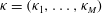 ${\it\kappa}=({\it\kappa}_{1},\ldots ,{\it\kappa}_{M})$
. In § 5, we develop a higher-order KP theory using the normal form theory. The goal of this section is to re-evaluate the previous numerical and experimental results. We then demonstrate that the KP theory revised with the higher-order correction provides an excellent model to describe Mach reflection phenomena. Finally, § 6 is devoted to the summary and conclusion.
${\it\kappa}=({\it\kappa}_{1},\ldots ,{\it\kappa}_{M})$
. In § 5, we develop a higher-order KP theory using the normal form theory. The goal of this section is to re-evaluate the previous numerical and experimental results. We then demonstrate that the KP theory revised with the higher-order correction provides an excellent model to describe Mach reflection phenomena. Finally, § 6 is devoted to the summary and conclusion.
2 Basic formulation
Consider water waves propagating over a horizontal bed in which the flow field is irrotational and incompressible, neglecting surface tension and assuming constant pressure along the air–water interface. Let us first denote the following scales:
 $$\begin{eqnarray}\left.\begin{array}{@{}c@{}}\displaystyle \tilde{{\it\lambda}}_{0}\sim \text{horizontal length scale}=\text{typical wave length},\\ \displaystyle \tilde{h}_{0}~\sim \text{vertical length scale}=\text{quiescent water depth},\\ \displaystyle \tilde{a}_{0}\sim \text{nonlinear scale}=\text{typical wave amplitude}.\end{array}\right\}\end{eqnarray}$$
Here, we consider shallow-water wave phenomena by setting
 $\tilde{h}_{0}\ll \tilde{{\it\lambda}}_{0}$
. The water surface elevation
$\tilde{h}_{0}\ll \tilde{{\it\lambda}}_{0}$
. The water surface elevation
 $\tilde{{\it\eta}}$
and the velocity potential
$\tilde{{\it\eta}}$
and the velocity potential
 $\tilde{{\it\phi}}$
and independent variables
$\tilde{{\it\phi}}$
and independent variables
 $(\tilde{x},{\tilde{y}},\tilde{z},\tilde{t})$
are non-dimensionalized as
$(\tilde{x},{\tilde{y}},\tilde{z},\tilde{t})$
are non-dimensionalized as
 $$\begin{eqnarray}\left.\begin{array}{@{}l@{}}\displaystyle \tilde{x}=\tilde{{\it\lambda}}_{0}x,\quad {\tilde{y}}=\tilde{{\it\lambda}}_{0}y,\quad \tilde{z}=\tilde{h}_{0}z,\quad \tilde{t}=\frac{\tilde{{\it\lambda}}_{0}}{\tilde{c}_{0}}t,\\ \displaystyle \tilde{{\it\eta}}=\tilde{a}_{0}{\it\eta},\quad \tilde{{\it\phi}}=\frac{\tilde{a}_{0}}{\tilde{h}_{0}}\tilde{{\it\lambda}}_{0}\tilde{c}_{0}{\it\phi},\end{array}\right\}\end{eqnarray}$$
where
 $\tilde{c}_{0}=\sqrt{\tilde{g}\tilde{h}_{0}}$
, in which
$\tilde{c}_{0}=\sqrt{\tilde{g}\tilde{h}_{0}}$
, in which
 $\tilde{g}$
is the gravitational acceleration and the corresponding non-dimensional variables are
$\tilde{g}$
is the gravitational acceleration and the corresponding non-dimensional variables are
 $\{x,y,z,t,{\it\eta},{\it\phi}\}$
with
$\{x,y,z,t,{\it\eta},{\it\phi}\}$
with
 $z$
pointing vertically upward from the bed and
$z$
pointing vertically upward from the bed and
 $(x,y)$
being the horizontal coordinates.
$(x,y)$
being the horizontal coordinates.
The shallow-water wave equation in the non-dimensional form is then expressed as
 $$\begin{eqnarray}\displaystyle \left.\begin{array}{@{}rl@{}}\,\,\,{\it\phi}_{zz}+{\it\beta}{\rm\Delta}{\it\phi}=0\quad & \text{for }0<z<1+{\it\alpha}{\it\eta},\\ \,\,\,{\it\phi}_{z}=0\quad & \text{at }z=0,\\ \end{array}\right\} & & \displaystyle\end{eqnarray}$$
 $$\begin{eqnarray}\displaystyle \left.\begin{array}{@{}l@{}}\displaystyle {\it\phi}_{t}+\frac{1}{2}{\it\alpha}|\boldsymbol{{\rm\nabla}}{\it\phi}|^{2}+\frac{1}{2}\frac{{\it\alpha}}{{\it\beta}}{\it\phi}_{z}^{2}+{\it\eta}=0\\ \displaystyle {\it\eta}_{t}+{\it\alpha}\boldsymbol{{\rm\nabla}}{\it\phi}\boldsymbol{\cdot }\boldsymbol{{\rm\nabla}}{\it\eta}=\frac{1}{{\it\beta}}{\it\phi}_{z}\end{array}\right\}\quad \text{at }z=1+{\it\alpha}{\it\eta}, & & \displaystyle\end{eqnarray}$$
 $\boldsymbol{{\rm\nabla}}=(\partial /\partial x,\partial /\partial y)$
and
$\boldsymbol{{\rm\nabla}}=(\partial /\partial x,\partial /\partial y)$
and
 ${\it\Delta}={\rm\nabla}^{2}$
is the two-dimensional Laplace operator for
${\it\Delta}={\rm\nabla}^{2}$
is the two-dimensional Laplace operator for
 $(x,y)$
. The parameters
$(x,y)$
. The parameters
 ${\it\alpha}$
and
${\it\alpha}$
and
 ${\it\beta}$
are
${\it\beta}$
are  $$\begin{eqnarray}{\it\alpha}=\frac{\tilde{a}_{0}}{\tilde{h}_{0}}\quad \text{and}\quad {\it\beta}=\left(\frac{\tilde{h}_{0}}{\tilde{{\it\lambda}}_{0}}\right)^{2}.\end{eqnarray}$$
The weak nonlinearity implies
 ${\it\alpha}\ll 1$
and the weak dispersion (or long-wave assumption) implies
${\it\alpha}\ll 1$
and the weak dispersion (or long-wave assumption) implies
 ${\it\beta}\ll 1$
, and we assume
${\it\beta}\ll 1$
, and we assume
 ${\it\alpha}\sim {\it\beta}=O({\it\epsilon})$
with a small parameter
${\it\alpha}\sim {\it\beta}=O({\it\epsilon})$
with a small parameter
 ${\it\epsilon}\ll 1$
.
${\it\epsilon}\ll 1$
.
From the first two equations of (2.3a
),
 ${\it\phi}$
can be written as
${\it\phi}$
can be written as
 $$\begin{eqnarray}{\it\phi}(x,y,z,t)=\cos (z\sqrt{{\it\beta}{\it\Delta}}){\it\psi}={\it\psi}-{\it\beta}\frac{z^{2}}{2}{\rm\Delta}{\it\psi}+{\it\beta}^{2}\frac{z^{4}}{24}{\it\Delta}^{2}{\it\psi}+O({\it\epsilon}^{3}),\end{eqnarray}$$
where
 ${\it\psi}(x,y,t)={\it\phi}(x,y,0,t)$
. Then the equations at the water surface
${\it\psi}(x,y,t)={\it\phi}(x,y,0,t)$
. Then the equations at the water surface
 $z=1+{\it\alpha}{\it\eta}$
give a Boussinesq-type system,
$z=1+{\it\alpha}{\it\eta}$
give a Boussinesq-type system,
 $$\begin{eqnarray}\displaystyle & & \displaystyle {\it\psi}_{t}+{\it\eta}+\frac{{\it\alpha}}{2}|\boldsymbol{{\rm\nabla}}{\it\psi}|^{2}-\frac{{\it\beta}}{2}{\rm\Delta}{\it\psi}_{t}\nonumber\\ \displaystyle & & \displaystyle \quad +\,\frac{{\it\alpha}{\it\beta}}{2}(({\rm\Delta}{\it\psi})^{2}+\boldsymbol{{\rm\nabla}}{\it\psi}\boldsymbol{\cdot }\boldsymbol{{\rm\nabla}}({\rm\Delta}{\it\psi})-2{\it\eta}{\rm\Delta}{\it\psi}_{t})+\frac{{\it\beta}^{2}}{24}{\it\Delta}^{2}{\it\psi}_{t}=O({\it\epsilon}^{3}),\end{eqnarray}$$
 $$\begin{eqnarray}\displaystyle & & \displaystyle {\it\eta}_{t}+{\rm\Delta}{\it\psi}+{\it\alpha}\boldsymbol{{\rm\nabla}}\boldsymbol{\cdot }({\it\eta}\boldsymbol{{\rm\nabla}}{\it\psi})-{\it\beta}\frac{1}{6}{\it\Delta}^{2}{\it\psi}\nonumber\\ \displaystyle & & \displaystyle \quad -\,\frac{{\it\alpha}{\it\beta}}{2}(\boldsymbol{{\rm\nabla}}{\it\eta}\boldsymbol{\cdot }\boldsymbol{{\rm\nabla}}({\rm\Delta}{\it\psi})+{\it\eta}{\it\Delta}^{2}{\it\psi})+\frac{{\it\beta}^{2}}{120}{\it\Delta}^{3}{\it\psi}=O({\it\epsilon}^{3}).\end{eqnarray}$$
We now derive the KP equation with the higher-order correction, which turns out to be key for physical applications, as we will discuss in § 5. The KP equation is based on the assumption of a weak dependence in the
 $y$
direction while
$y$
direction while
 $x$
denotes the predominant wave propagation direction (i.e. quasi-two-dimensionality). Introducing a small parameter
$x$
denotes the predominant wave propagation direction (i.e. quasi-two-dimensionality). Introducing a small parameter
 ${\it\gamma}$
, the
${\it\gamma}$
, the
 $y$
coordinate is scaled as
$y$
coordinate is scaled as
 $$\begin{eqnarray}{\it\zeta}:=\sqrt{{\it\gamma}}y,\quad \text{with }{\it\gamma}=O({\it\epsilon}).\end{eqnarray}$$
Translating coordinates of the reference frame
 ${\it\xi}=x-t$
, introducing the slow time scale
${\it\xi}=x-t$
, introducing the slow time scale
 ${\it\tau}={\it\epsilon}t$
and eliminating
${\it\tau}={\it\epsilon}t$
and eliminating
 ${\it\eta}$
in the equations (2.6) and (2.7) yield the KP equation for
${\it\eta}$
in the equations (2.6) and (2.7) yield the KP equation for
 $v:={\it\psi}_{{\it\xi}}({\it\xi},{\it\zeta},{\it\tau})$
with higher-order corrections up to
$v:={\it\psi}_{{\it\xi}}({\it\xi},{\it\zeta},{\it\tau})$
with higher-order corrections up to
 $O({\it\epsilon}^{2})$
,
$O({\it\epsilon}^{2})$
,
 $$\begin{eqnarray}\displaystyle & & \displaystyle 2{\it\epsilon}v_{{\it\tau}}+3{\it\alpha}vv_{{\it\xi}}+\frac{{\it\beta}}{3}v_{{\it\xi}{\it\xi}{\it\xi}}+{\it\gamma}D^{-1}v_{{\it\zeta}{\it\zeta}}\nonumber\\ \displaystyle & & \displaystyle \quad +\,\frac{19}{180}{\it\beta}^{2}v_{{\it\xi}{\it\xi}{\it\xi}{\it\xi}{\it\xi}}+{\it\alpha}{\it\beta}\left(\frac{15}{6}vv_{{\it\xi}{\it\xi}{\it\xi}}+\frac{53}{12}v_{{\it\xi}}v_{{\it\xi}{\it\xi}}\right)+\frac{{\it\beta}{\it\gamma}}{2}v_{{\it\xi}{\it\zeta}{\it\zeta}}-\frac{{\it\gamma}^{2}}{4}D^{-3}v_{{\it\zeta}{\it\zeta}{\it\zeta}{\it\zeta}}\nonumber\\ \displaystyle & & \displaystyle \quad +\,{\it\alpha}{\it\gamma}\left(\frac{5}{4}vD^{-1}v_{{\it\zeta}{\it\zeta}}+2v_{{\it\zeta}}D^{-1}v_{{\it\zeta}}-\frac{3}{4}D^{-1}(v^{2})_{{\it\zeta}{\it\zeta}}+\frac{1}{2}v_{{\it\xi}}D^{-2}v_{{\it\zeta}{\it\zeta}}\right)=O({\it\epsilon}^{3}),\end{eqnarray}$$
where
 $D^{-1}:=\partial _{{\it\xi}}^{-1}$
is a formal integral operator with respect to
$D^{-1}:=\partial _{{\it\xi}}^{-1}$
is a formal integral operator with respect to
 ${\it\xi}$
. The first line of this equation of the order
${\it\xi}$
. The first line of this equation of the order
 $O({\it\epsilon})$
is the traditional KP equation, and the terms in the second and third lines are the
$O({\it\epsilon})$
is the traditional KP equation, and the terms in the second and third lines are the
 $O({\it\epsilon}^{2})$
correction. The water surface
$O({\it\epsilon}^{2})$
correction. The water surface
 ${\it\eta}$
is expressed as
${\it\eta}$
is expressed as
 $$\begin{eqnarray}{\it\eta}=v+\frac{{\it\alpha}}{4}v^{2}-\frac{{\it\beta}}{3}v_{{\it\xi}{\it\xi}}+\frac{{\it\gamma}}{2}D^{-2}v_{{\it\zeta}{\it\zeta}}+O({\it\epsilon}^{2}).\end{eqnarray}$$
Next, we transform (2.9) into a canonical form of the KP equation with the change of variables,
 $$\begin{eqnarray}{\it\xi}=\sqrt{{\it\beta}}\,X,\quad {\it\zeta}=\sqrt{{\it\beta}{\it\gamma}}\,Y,\quad {\it\tau}=\frac{3{\it\epsilon}\sqrt{{\it\beta}}}{2}\,T,\quad v=\frac{2}{3{\it\alpha}}u.\end{eqnarray}$$
Then (2.9) becomes
 $$\begin{eqnarray}\displaystyle -4u_{T} & = & \displaystyle 6uu_{X}+u_{XXX}+3D^{-1}u_{YY}\nonumber\\ \displaystyle & & \displaystyle +\,{\textstyle \frac{19}{60}}u_{XXXXX}+{\textstyle \frac{5}{3}}uu_{XXX}+{\textstyle \frac{53}{6}}u_{X}u_{XX}+{\textstyle \frac{3}{2}}u_{XYY}-{\textstyle \frac{3}{4}}D^{-3}u_{YYYY}\nonumber\\ \displaystyle & & \displaystyle +\,{\textstyle \frac{5}{2}}uD^{-1}u_{YY}+4u_{Y}D^{-1}u_{Y}-{\textstyle \frac{3}{4}}D^{-1}(u^{2})_{YY}+u_{X}D^{-2}u_{YY}+O({\it\epsilon}^{9/2}),\end{eqnarray}$$
which we refer to as the higher-order KP equation. Here we have the orders
 $u\sim O({\it\epsilon})$
,
$u\sim O({\it\epsilon})$
,
 $\partial _{X}\sim O({\it\epsilon}^{1/2})$
,
$\partial _{X}\sim O({\it\epsilon}^{1/2})$
,
 $D^{-1}\sim O({\it\epsilon}^{-1/2})$
and
$D^{-1}\sim O({\it\epsilon}^{-1/2})$
and
 $\partial _{Y}\sim O({\it\epsilon})$
. Note that the new variables
$\partial _{Y}\sim O({\it\epsilon})$
. Note that the new variables
 $(X,Y,T)$
are related to the physical ones via
$(X,Y,T)$
are related to the physical ones via
 $$\begin{eqnarray}\tilde{x}-\tilde{c}_{0}\tilde{t}=\tilde{h}_{0}X,\quad {\tilde{y}}=\tilde{h}_{0}\,Y,\quad \tilde{t}=\frac{3\tilde{h}_{0}}{2\tilde{c}_{0}}\,T.\end{eqnarray}$$
The water surface elevation
 ${\it\eta}$
in terms of
${\it\eta}$
in terms of
 $u$
is given by
$u$
is given by
 $$\begin{eqnarray}{\it\alpha}{\it\eta}={\textstyle \frac{2}{3}}u+{\textstyle \frac{1}{9}}u^{2}-{\textstyle \frac{2}{9}}u_{XX}+{\textstyle \frac{1}{3}}D^{-2}u_{YY}+O({\it\epsilon}^{3}).\end{eqnarray}$$
In the leading-order approximation, the physical water surface
 ${\it\alpha}{\it\eta}$
is expressed by
${\it\alpha}{\it\eta}$
is expressed by
 ${\it\alpha}{\it\eta}=2u/3$
with the KP water surface parameter
${\it\alpha}{\it\eta}=2u/3$
with the KP water surface parameter
 $u$
. Hereafter, we use the lower case letters
$u$
. Hereafter, we use the lower case letters
 $(x,y,t)$
for
$(x,y,t)$
for
 $(X,Y,T)$
, and the KP variables can be converted to the physical variables
$(X,Y,T)$
, and the KP variables can be converted to the physical variables
 $(\tilde{x},{\tilde{y}},\tilde{t})$
and
$(\tilde{x},{\tilde{y}},\tilde{t})$
and
 $\tilde{{\it\eta}}=\tilde{h}_{0}{\it\alpha}{\it\eta}$
directly through the relations (2.13).
$\tilde{{\it\eta}}=\tilde{h}_{0}{\it\alpha}{\it\eta}$
directly through the relations (2.13).
3 The KP solitons
A brief summary of soliton solutions of the KP equation is given here, while we refer to Chakravarty & Kodama (Reference Chakravarty and Kodama2009) and Kodama (Reference Kodama2004, Reference Kodama2010) for detailed discussions. The canonical form of the KP equation is the first line of (2.12):
 $$\begin{eqnarray}4u_{t}+6uu_{x}+u_{xxx}+3D^{-1}u_{yy}=0.\end{eqnarray}$$
The solution is represented in the
 ${\it\tau}$
-function form,
${\it\tau}$
-function form,
 $$\begin{eqnarray}u(x,y,t)=2\partial _{x}^{2}\ln {\it\tau}(x,y,t).\end{eqnarray}$$
For soliton solutions, we consider the
 ${\it\tau}$
function in the Wronskian determinant with
${\it\tau}$
function in the Wronskian determinant with
 $N$
functions
$N$
functions
 $f_{n}$
for
$f_{n}$
for
 $n=1,\ldots ,N$
(see, for example, Matveev Reference Matveev1979; Satsuma Reference Satsuma1979; Freeman & Nimmo Reference Freeman and Nimmo1983; Hirota Reference Hirota2004),
$n=1,\ldots ,N$
(see, for example, Matveev Reference Matveev1979; Satsuma Reference Satsuma1979; Freeman & Nimmo Reference Freeman and Nimmo1983; Hirota Reference Hirota2004),
 $$\begin{eqnarray}{\it\tau}=Wr(f_{1},f_{2},\ldots ,f_{N}).\end{eqnarray}$$
The functions
 $\{f_{1},\ldots ,f_{N}\}$
form a set of independent solutions of the linear equations,
$\{f_{1},\ldots ,f_{N}\}$
form a set of independent solutions of the linear equations,
 $$\begin{eqnarray}\partial _{y}f_{n}=\partial _{x}^{2}f_{n},\quad \partial _{t}\,f_{n}=-\partial _{x}^{3}f_{n}.\end{eqnarray}$$
In particular, we consider a set of solutions in finite Fourier series,
 $$\begin{eqnarray}f_{n}(x,y,t)=\mathop{\sum }_{m=1}^{M}a_{n,m}E_{m}(x,y,t)\quad \text{with }E_{m}=e^{{\it\theta}_{m}}:=\exp ({\it\kappa}_{m}x+{\it\kappa}_{m}^{2}y-{\it\kappa}_{m}^{3}t).\end{eqnarray}$$
Thus this type of solution is characterized by the ordered
 ${\it\kappa}$
parameters
${\it\kappa}$
parameters
 $\{{\it\kappa}_{1}<\cdots <{\it\kappa}_{M}\}$
and the
$\{{\it\kappa}_{1}<\cdots <{\it\kappa}_{M}\}$
and the
 $N\times M$
matrix
$N\times M$
matrix
 $\unicode[STIX]{x1D63C}:=(a_{n,m})$
of rank
$\unicode[STIX]{x1D63C}:=(a_{n,m})$
of rank
 $(A)=N$
, so that
$(A)=N$
, so that
 $$\begin{eqnarray}(f_{1},f_{2},\ldots ,f_{N})=(E_{1},E_{2},\ldots ,E_{M})\unicode[STIX]{x1D63C}^{\text{T}}.\end{eqnarray}$$
Note here that if we use other set
 $(g_{1},\ldots ,g_{N})=(f_{1},\ldots ,f_{N})H$
for any
$(g_{1},\ldots ,g_{N})=(f_{1},\ldots ,f_{N})H$
for any
 $H\in \text{GL}_{N}(\mathbb{R})$
, (
$H\in \text{GL}_{N}(\mathbb{R})$
, (
 $\text{GL}_{N}(\mathbb{R})$
is the general linear group of rank
$\text{GL}_{N}(\mathbb{R})$
is the general linear group of rank
 $N$
), then the
$N$
), then the
 ${\it\tau}$
function changes only by the constant factor of
${\it\tau}$
function changes only by the constant factor of
 $\text{det}(H)$
. That is, the solution remains the same under this transform with GL
$\text{det}(H)$
. That is, the solution remains the same under this transform with GL
 $_{N}(\mathbb{R})$
, and this freedom in the
$_{N}(\mathbb{R})$
, and this freedom in the
 $\unicode[STIX]{x1D63C}$
matrix can be fixed by expressing
$\unicode[STIX]{x1D63C}$
matrix can be fixed by expressing
 $\unicode[STIX]{x1D63C}$
in the reduced row echelon form.
$\unicode[STIX]{x1D63C}$
in the reduced row echelon form.
Now using the Binet–Cauchy Lemma for the determinant, the
 ${\it\tau}$
function of (3.3) can be expressed in the form
${\it\tau}$
function of (3.3) can be expressed in the form
 $$\begin{eqnarray}\displaystyle {\it\tau}(x,y,t)=\mathop{\sum }_{1\leqslant j_{1}<\cdots <j_{N}\leqslant M}{\it\Delta}_{j_{1},\ldots ,j_{N}}(A)E_{j_{1},\ldots ,j_{N}}(x,y,t), & & \displaystyle\end{eqnarray}$$
where
 ${\it\Delta}_{j_{1},\ldots ,j_{N}}(A)$
is the
${\it\Delta}_{j_{1},\ldots ,j_{N}}(A)$
is the
 $N\times N$
minor of the
$N\times N$
minor of the
 $\unicode[STIX]{x1D63C}$
matrix with
$\unicode[STIX]{x1D63C}$
matrix with
 $N$
columns marked by
$N$
columns marked by
 $\{j_{1},\ldots ,j_{N}\}$
and
$\{j_{1},\ldots ,j_{N}\}$
and
 $E_{j_{1},\ldots ,j_{N}}(x,y,t)$
is given by
$E_{j_{1},\ldots ,j_{N}}(x,y,t)$
is given by
 $$\begin{eqnarray}E_{j_{1},\ldots ,j_{N}}(x,y,t)=Wr(E_{j_{1}},\ldots ,E_{j_{N}})=\mathop{\prod }_{l<m}({\it\kappa}_{j_{m}}-{\it\kappa}_{j_{l}})E_{j_{1}}\cdots E_{j_{N}}.\end{eqnarray}$$
Note that we are interested in non-singular solutions. Since the solution is given by
 $u=2\partial _{x}^{2}(\ln {\it\tau})$
, the non-singular solutions are obtained by imposing the non-negativity condition on the minors,
$u=2\partial _{x}^{2}(\ln {\it\tau})$
, the non-singular solutions are obtained by imposing the non-negativity condition on the minors,
 $$\begin{eqnarray}{\it\Delta}_{j_{1},\ldots ,j_{N}}(A)\geqslant 0,\quad \text{for all }1\leqslant j_{1}<\cdots <j_{N}\leqslant M.\end{eqnarray}$$
This condition is sufficient for non-singularity of the solution for any initial data (see Kodama & Williams (Reference Kodama and Williams2013) for the necessary condition for regularity). We call a matrix
 $\unicode[STIX]{x1D63C}$
having the condition (3.9) a totally non-negative matrix.
$\unicode[STIX]{x1D63C}$
having the condition (3.9) a totally non-negative matrix.
3.1 Soliton solutions and notations
One soliton solution is obtained by the
 ${\it\tau}$
function with
${\it\tau}$
function with
 $M=2$
and
$M=2$
and
 $N=1$
, i.e.
$N=1$
, i.e.
 ${\it\tau}=f_{1}=a_{11}E_{1}+a_{12}E_{2}$
with
${\it\tau}=f_{1}=a_{11}E_{1}+a_{12}E_{2}$
with
 $\unicode[STIX]{x1D63C}=(a_{11}~a_{12})$
. Since the solution
$\unicode[STIX]{x1D63C}=(a_{11}~a_{12})$
. Since the solution
 $u$
is given by (3.2), one can take
$u$
is given by (3.2), one can take
 $a_{11}=1$
and denote
$a_{11}=1$
and denote
 $a_{12}=a>0$
. Then we have
$a_{12}=a>0$
. Then we have
 $$\begin{eqnarray}u=2\partial _{x}^{2}\ln {\it\tau}={\textstyle \frac{1}{2}}({\it\kappa}_{1}-{\it\kappa}_{2})^{2}\,\text{sech}^{2}{\textstyle \frac{1}{2}}({\it\theta}_{1}-{\it\theta}_{2}-\ln a),\end{eqnarray}$$
of which the solution is localized along the line
 ${\it\theta}_{1}-{\it\theta}_{2}=\ln a$
. Note that the line soliton appears at the boundary of two regions in the
${\it\theta}_{1}-{\it\theta}_{2}=\ln a$
. Note that the line soliton appears at the boundary of two regions in the
 $xy$
plane where either
$xy$
plane where either
 $E_{1}$
or
$E_{1}$
or
 $E_{2}$
is the dominant exponential term, and because of this we call this soliton a [1,2]-soliton solution. Likewise, we refer to each of these asymptotic line solitons as the
$E_{2}$
is the dominant exponential term, and because of this we call this soliton a [1,2]-soliton solution. Likewise, we refer to each of these asymptotic line solitons as the
 $[i,j]$
-soliton with
$[i,j]$
-soliton with
 $i<j$
whose
$i<j$
whose
 ${\it\tau}$
function around the soliton can be expressed by
${\it\tau}$
function around the soliton can be expressed by
 ${\it\tau}\approx {\it\Delta}_{I}E_{I}+{\it\Delta}_{J}E_{J}$
with the index sets
${\it\tau}\approx {\it\Delta}_{I}E_{I}+{\it\Delta}_{J}E_{J}$
with the index sets
 $I$
containing
$I$
containing
 $i$
and
$i$
and
 $J$
containing
$J$
containing
 $j$
, which satisfy
$j$
, which satisfy
 $I\setminus \{i\}=J\setminus \{j\}$
. The
$I\setminus \{i\}=J\setminus \{j\}$
. The
 $[i,j]$
-soliton solution has the same local structure as the one-soliton solution and can be described as follows
$[i,j]$
-soliton solution has the same local structure as the one-soliton solution and can be described as follows
 $$\begin{eqnarray}u=A_{[i,j]}\,\text{sech}^{2}{\textstyle \frac{1}{2}}(\boldsymbol{K}_{[i,j]}\boldsymbol{\cdot }\boldsymbol{x}-{\it\Omega}_{[i,j]}t+{\it\Theta}_{[i,j]}^{0}),\end{eqnarray}$$
with some constant
 ${\it\Theta}_{[i,j]}^{0}$
. The amplitude
${\it\Theta}_{[i,j]}^{0}$
. The amplitude
 $A_{[i,j]}$
, the wavenumber vector
$A_{[i,j]}$
, the wavenumber vector
 $\boldsymbol{K}_{[i,j]}$
and the frequency
$\boldsymbol{K}_{[i,j]}$
and the frequency
 ${\it\Omega}_{[i,j]}$
are expressed by
${\it\Omega}_{[i,j]}$
are expressed by
 $$\begin{eqnarray}A_{[i,j]}={\textstyle \frac{1}{2}}({\it\kappa}_{j}-{\it\kappa}_{i})^{2},\quad \boldsymbol{K}_{[i,j]}=({\it\kappa}_{j}-{\it\kappa}_{i},{\it\kappa}_{j}^{2}-{\it\kappa}_{i}^{2}),\quad {\it\Omega}_{[i,j]}={\it\kappa}_{j}^{3}-{\it\kappa}_{i}^{3}.\end{eqnarray}$$
The direction of the wavenumber vector
 $\boldsymbol{K}_{[i,j]}=(K_{[i,j]}^{x},K_{[i,j]}^{y})$
is measured in the counterclockwise direction from the
$\boldsymbol{K}_{[i,j]}=(K_{[i,j]}^{x},K_{[i,j]}^{y})$
is measured in the counterclockwise direction from the
 $y$
axis and it is given by
$y$
axis and it is given by
 $$\begin{eqnarray}\frac{K_{[i,j]}^{y}}{K_{[i,j]}^{x}}=\tan {\it\Psi}_{[i,j]}={\it\kappa}_{i}+{\it\kappa}_{j},\end{eqnarray}$$
that is,
 ${\it\Psi}_{[i,j]}$
gives the angle between the line
${\it\Psi}_{[i,j]}$
gives the angle between the line
 $\boldsymbol{K}_{[i,j]}\boldsymbol{\cdot }\boldsymbol{x}=\text{const.}$
and the
$\boldsymbol{K}_{[i,j]}\boldsymbol{\cdot }\boldsymbol{x}=\text{const.}$
and the
 $y$
axis (see figure 1). Note that
$y$
axis (see figure 1). Note that
 $\boldsymbol{K}_{[i,j]}$
and
$\boldsymbol{K}_{[i,j]}$
and
 ${\it\Omega}_{[i,j]}$
satisfy the soliton-dispersion relation,
${\it\Omega}_{[i,j]}$
satisfy the soliton-dispersion relation,
 $$\begin{eqnarray}4{\it\Omega}_{[i,j]}K_{[i,j]}^{x}=(K_{[i,j]}^{x})^{4}+3(K_{[i,j]}^{y})^{2}.\end{eqnarray}$$
The crest line of
 $[i,j]$
-soliton is given by
$[i,j]$
-soliton is given by
 $\boldsymbol{K}_{[i,j]}\boldsymbol{\cdot }\boldsymbol{x}-{\it\Omega}_{[i,j]}t+{\it\Theta}_{[i,j]}^{0}=0$
, i.e.
$\boldsymbol{K}_{[i,j]}\boldsymbol{\cdot }\boldsymbol{x}-{\it\Omega}_{[i,j]}t+{\it\Theta}_{[i,j]}^{0}=0$
, i.e.
 $$\begin{eqnarray}x+\tan {\it\Psi}_{[i,j]}y-V_{[i,j]}t=x_{0}\quad \text{with }V_{[i,j]}=\frac{{\it\kappa}_{i}^{3}-{\it\kappa}_{j}^{3}}{{\it\kappa}_{i}-{\it\kappa}_{j}}={\it\kappa}_{i}^{2}+{\it\kappa}_{i}{\it\kappa}_{j}+{\it\kappa}_{j}^{2},\end{eqnarray}$$
for some constant
 $x_{0}$
. Note
$x_{0}$
. Note
 $V_{[i,j]}>0$
, that is, each soliton propagates in the positive
$V_{[i,j]}>0$
, that is, each soliton propagates in the positive
 $x$
direction, which is important when we set-up the coordinates for a laboratory or numerical experiment of shallow-water waves.
$x$
direction, which is important when we set-up the coordinates for a laboratory or numerical experiment of shallow-water waves.

Figure 1. One line-soliton solution of
 $[i,j]$
-type and the corresponding chord diagram. The upper oriented chord represents the part of
$[i,j]$
-type and the corresponding chord diagram. The upper oriented chord represents the part of
 $[i,j]$
-soliton for
$[i,j]$
-soliton for
 $y\gg 0$
and the lower one for
$y\gg 0$
and the lower one for
 $y\ll 0$
. The middle line of the chord diagram shows the coordinate axis for the
$y\ll 0$
. The middle line of the chord diagram shows the coordinate axis for the
 ${\it\kappa}$
parameters. Notice that the wave amplitude is represented by
${\it\kappa}$
parameters. Notice that the wave amplitude is represented by
 $A_{[i,j]}=({\it\kappa}_{j}-{\it\kappa}_{i})^{2}/2$
and the counterclockwise shift of the wave propagation is expressed by
$A_{[i,j]}=({\it\kappa}_{j}-{\it\kappa}_{i})^{2}/2$
and the counterclockwise shift of the wave propagation is expressed by
 $\tan {\it\Psi}_{[i,j]}={\it\kappa}_{i}+{\it\kappa}_{j}$
, which is positive for this example.
$\tan {\it\Psi}_{[i,j]}={\it\kappa}_{i}+{\it\kappa}_{j}$
, which is positive for this example.
In figure 1, we illustrate one line-soliton solution of
 $[i,j]$
-type. In the right panel of this figure, we show a chord diagram which represents this single line-soliton solution. The chord diagram is a product of the KP analysis made by Chakravarty & Kodama (Reference Chakravarty and Kodama2009), which represents the asymptotic soliton solutions for
$[i,j]$
-type. In the right panel of this figure, we show a chord diagram which represents this single line-soliton solution. The chord diagram is a product of the KP analysis made by Chakravarty & Kodama (Reference Chakravarty and Kodama2009), which represents the asymptotic soliton solutions for
 $y\rightarrow \pm \infty$
.
$y\rightarrow \pm \infty$
.
Now we describe some exact soliton solutions of the KP equation for two line solitons. For two interacting line solitons, the matrix
 $\unicode[STIX]{x1D63C}=(a_{ij})$
is a constant
$\unicode[STIX]{x1D63C}=(a_{ij})$
is a constant
 $2\times 4$
matrix and each solution
$2\times 4$
matrix and each solution
 $u(x,y,t)$
is determined by the
$u(x,y,t)$
is determined by the
 $\unicode[STIX]{x1D63C}$
matrix and the
$\unicode[STIX]{x1D63C}$
matrix and the
 ${\it\kappa}$
parameters. From (3.7), the
${\it\kappa}$
parameters. From (3.7), the
 ${\it\tau}$
function can be written as
${\it\tau}$
function can be written as
 $$\begin{eqnarray}\displaystyle {\it\tau}(x,y,t)=\mathop{\sum }_{1\leqslant i<j\leqslant 4}{\it\Delta}_{i,j}(A)E_{i,j}(x,y,t), & & \displaystyle\end{eqnarray}$$
where
 ${\it\Delta}_{i,j}(A)$
is the
${\it\Delta}_{i,j}(A)$
is the
 $2\times 2$
minors consisting of
$2\times 2$
minors consisting of
 $i$
th and
$i$
th and
 $j$
th columns of the
$j$
th columns of the
 $2\times 4$
 $\unicode[STIX]{x1D63C}$
-matrix, and
$\unicode[STIX]{x1D63C}$
-matrix, and
 $E_{i,j}=Wr(e^{{\it\theta}_{i}},e^{{\it\theta}_{j}})=({\it\kappa}_{j}-{\it\kappa}_{i})e^{{\it\theta}_{i}+{\it\theta}_{j}}$
(note
$E_{i,j}=Wr(e^{{\it\theta}_{i}},e^{{\it\theta}_{j}})=({\it\kappa}_{j}-{\it\kappa}_{i})e^{{\it\theta}_{i}+{\it\theta}_{j}}$
(note
 $E_{i,j}>0$
with the order
$E_{i,j}>0$
with the order
 ${\it\kappa}_{i}<{\it\kappa}_{j}$
). As shown by Chakravarty & Kodama (Reference Chakravarty and Kodama2009),
${\it\kappa}_{i}<{\it\kappa}_{j}$
). As shown by Chakravarty & Kodama (Reference Chakravarty and Kodama2009),
 ${\it\tau}$
function (3.15) generates a soliton solution that consists of two line solitons for
${\it\tau}$
function (3.15) generates a soliton solution that consists of two line solitons for
 $y\rightarrow \pm \infty$
. We call this type soliton solution a (2,2)-soliton solution. In general, an
$y\rightarrow \pm \infty$
. We call this type soliton solution a (2,2)-soliton solution. In general, an
 $(N_{-},N_{+})$
soliton means that the solution has
$(N_{-},N_{+})$
soliton means that the solution has
 $N_{-}$
asymptotic line solitons for
$N_{-}$
asymptotic line solitons for
 $y\ll 0$
and
$y\ll 0$
and
 $N_{+}$
asymptotic line solitons for
$N_{+}$
asymptotic line solitons for
 $y\gg 0$
. Those asymptotic soliton solutions can be parameterized by the permutations, which lead to the chord diagram to express the classification of soliton solutions as a chord joining a pair of parameters
$y\gg 0$
. Those asymptotic soliton solutions can be parameterized by the permutations, which lead to the chord diagram to express the classification of soliton solutions as a chord joining a pair of parameters
 ${\it\kappa}_{j}$
following the permutation. Figure 2 shows seven possible types of
${\it\kappa}_{j}$
following the permutation. Figure 2 shows seven possible types of
 $(2,2)$
-soliton solutions for
$(2,2)$
-soliton solutions for
 $2\times 4$
matrix
$2\times 4$
matrix
 $\unicode[STIX]{x1D63C}$
. For example, the chord diagram of
$\unicode[STIX]{x1D63C}$
. For example, the chord diagram of
 $(3142)$
-type soliton shows that there are [1,3]- and [3,4]-solitons for
$(3142)$
-type soliton shows that there are [1,3]- and [3,4]-solitons for
 $y\gg 0$
and [1,2]- and [2,4]-solitons for
$y\gg 0$
and [1,2]- and [2,4]-solitons for
 $y\ll 0$
. Detailed mathematical descriptions are given by Chakravarty & Kodama (Reference Chakravarty and Kodama2009).
$y\ll 0$
. Detailed mathematical descriptions are given by Chakravarty & Kodama (Reference Chakravarty and Kodama2009).

Figure 2. The chord diagrams for seven different types of (2, 2)-soliton solutions. The number in the parenthesis represents the permutation. After Chakravarty & Kodama (Reference Chakravarty and Kodama2009).
4 Mach reflection
Miles (Reference Miles1977a
,Reference Miles
b
) analysed obliquely incident solitons onto a reflective boundary (i.e. vertical wall). Although he did not explicitly use the KP equation, his analysis led to solutions equivalent to the KP theory under the assumptions of weak nonlinearity and small incident angle. Miles found that there exists an angle
 ${\it\Psi}_{c}$
such that, if the incidence angle
${\it\Psi}_{c}$
such that, if the incidence angle
 ${\it\Psi}_{0}$
is larger than
${\it\Psi}_{0}$
is larger than
 ${\it\Psi}_{c}$
, the reflected wave behind the incidence wave has the same angle
${\it\Psi}_{c}$
, the reflected wave behind the incidence wave has the same angle
 ${\it\Psi}_{0}$
with a phase shift at the intersection. If the angle is smaller than
${\it\Psi}_{0}$
with a phase shift at the intersection. If the angle is smaller than
 ${\it\Psi}_{c}$
, then the Mach stem appears and continually grows its crest length, as illustrated in figure 3.
${\it\Psi}_{c}$
, then the Mach stem appears and continually grows its crest length, as illustrated in figure 3.

Figure 3. The Mach reflection. The lower part of (a) corresponds to the mirror image of the upper part of the experimental waves. (b) Illustrates an equivalent system to the experiment. The resulting wave pattern in (b) shown is a
 $(3142)$
-soliton solution (see the text for the details). For a
$(3142)$
-soliton solution (see the text for the details). For a
 $(2143)$
-soliton solution, the angle
$(2143)$
-soliton solution, the angle
 ${\it\Phi}$
becomes zero if the initial angle satisfies
${\it\Phi}$
becomes zero if the initial angle satisfies
 ${\it\Psi}_{0}\geqslant {\it\Psi}_{c}$
, i.e. no stem formation.
${\it\Psi}_{0}\geqslant {\it\Psi}_{c}$
, i.e. no stem formation.
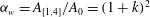
The incident wave, the reflected wave and the Mach stem interact and form a resonant triad. Miles’s prediction for the maximum wave amplification
 ${\it\alpha}_{w}$
– the ratio of the wave amplitude at the wall
${\it\alpha}_{w}$
– the ratio of the wave amplitude at the wall
 $a_{w}$
to the incident wave amplitude
$a_{w}$
to the incident wave amplitude
 $a_{0}$
(
$a_{0}$
(
 $=\tilde{a}_{0}/\tilde{h}_{0}$
) – is expressed as
$=\tilde{a}_{0}/\tilde{h}_{0}$
) – is expressed as
 $$\begin{eqnarray}{\it\alpha}_{w}:=\frac{a_{w}}{a_{0}}=\left\{\begin{array}{@{}ll@{}}\displaystyle (1+k)^{2}, & \text{ for }k<1,\\ \displaystyle \frac{4}{1+\sqrt{1-k^{-2}}}, & \text{ for }k>1.\end{array}\right.\end{eqnarray}$$
where
 $k$
is the parameter defined by
$k$
is the parameter defined by
 $$\begin{eqnarray}k=\frac{{\it\Psi}_{0}}{\sqrt{3a_{0}}},\end{eqnarray}$$
in which
 ${\it\Psi}_{c}=\sqrt{3a_{0}}$
. Hereafter, we call
${\it\Psi}_{c}=\sqrt{3a_{0}}$
. Hereafter, we call
 $k$
in (4.2) the Miles parameter. Under the assumption of a small angle, Miles assumed that
$k$
in (4.2) the Miles parameter. Under the assumption of a small angle, Miles assumed that
 $\sin {\it\Psi}_{0}\approx {\it\Psi}_{0}$
, which turns out to be the key assumption that causes discrepancy between the predictions and the experiments: this will be discussed in § 4.2.
$\sin {\it\Psi}_{0}\approx {\it\Psi}_{0}$
, which turns out to be the key assumption that causes discrepancy between the predictions and the experiments: this will be discussed in § 4.2.
Miles derived (4.1) under the assumption of small incidence angle
 ${\it\Psi}_{0}$
, which is referred to as a strong interaction. In the case of large
${\it\Psi}_{0}$
, which is referred to as a strong interaction. In the case of large
 ${\it\Psi}_{0}$
(he assumed
${\it\Psi}_{0}$
(he assumed
 $\sin ^{2}{\it\Psi}_{0}\gg a_{0}$
), the following equation for the maximum amplification is obtained:
$\sin ^{2}{\it\Psi}_{0}\gg a_{0}$
), the following equation for the maximum amplification is obtained:
 $$\begin{eqnarray}{\it\alpha}_{w}=2+a_{0}\left(\frac{3}{2\sin ^{2}{\it\Psi}_{0}}-3+2\sin ^{2}{\it\Psi}_{0}\right).\end{eqnarray}$$
In § 5, we will show that (4.3) is well approximated by (4.1) for
 $k>1$
after modifying the parameter
$k>1$
after modifying the parameter
 $k$
with the higher-order correction. This means that (4.3) is smoothly connected to (4.1) for
$k$
with the higher-order correction. This means that (4.3) is smoothly connected to (4.1) for
 $k>1$
with the new parameter.
$k>1$
with the new parameter.
4.1 KP theory
Figure 4 illustrates the contour plots of (2143)-type and (3142)-type solutions of the KP theory in the
 $xy$
plane which are symmetric with respect to the
$xy$
plane which are symmetric with respect to the
 $x$
axis and the corresponding chord diagrams, respectively. Recall that the upper chords represent the asymptotic solitons
$x$
axis and the corresponding chord diagrams, respectively. Recall that the upper chords represent the asymptotic solitons
 $[i,j]$
for
$[i,j]$
for
 $y\gg 0$
and the lower chords the asymptotic solitons
$y\gg 0$
and the lower chords the asymptotic solitons
 $[i,j]$
for
$[i,j]$
for
 $y\ll 0$
. Let us fix the amplitudes
$y\ll 0$
. Let us fix the amplitudes
 $A_{[i,j]}$
and the angles
$A_{[i,j]}$
and the angles
 ${\it\Psi}_{[i,j]}$
of the solitons in the positive
${\it\Psi}_{[i,j]}$
of the solitons in the positive
 $x$
regions for both (2143)- and (3142)-types, so that those solutions are symmetric with respect to the
$x$
regions for both (2143)- and (3142)-types, so that those solutions are symmetric with respect to the
 $x$
axis:
$x$
axis:
 $$\begin{eqnarray}\displaystyle A_{0}=\left\{\begin{array}{@{}ll@{}}\displaystyle A_{[1,2]}=A_{[3,4]} & \quad (2143)\,\text{type}\\ \displaystyle A_{[1,3]}=A_{[2,4]} & \quad (3142)\,\text{type},\end{array}\right. & & \displaystyle\end{eqnarray}$$
 $$\begin{eqnarray}\displaystyle {\it\Psi}_{0}=\left\{\begin{array}{@{}ll@{}}\displaystyle -{\it\Psi}_{[1,2]}={\it\Psi}_{[3,4]}>0 & \quad (2143)\,\text{type}\\ \displaystyle -{\it\Psi}_{[1,3]}={\it\Psi}_{[2,4]}>0 & \quad (3142)\text{ type},\end{array}\right. & & \displaystyle\end{eqnarray}$$

Figure 4. Contour plots and chord diagrams. (a) (2143)-type solution. (b) (3142)-type solution. The length of [1,4]-soliton in the right figure changes in
 $t$
.
$t$
.
Then we express the
 ${\it\kappa}$
parameters in terms of
${\it\kappa}$
parameters in terms of
 $A_{0}$
and
$A_{0}$
and
 $\tan {\it\Psi}_{0}$
with
$\tan {\it\Psi}_{0}$
with
 ${\it\kappa}_{1}=-{\it\kappa}_{4}$
and
${\it\kappa}_{1}=-{\it\kappa}_{4}$
and
 ${\it\kappa}_{2}=-{\it\kappa}_{3}$
(due to the symmetry). In the case of (2143)-type. With the use of (3.11a
) and (3.12), we have
${\it\kappa}_{2}=-{\it\kappa}_{3}$
(due to the symmetry). In the case of (2143)-type. With the use of (3.11a
) and (3.12), we have
 $$\begin{eqnarray}{\it\kappa}_{1}=-{\textstyle \frac{1}{2}}(\tan {\it\Psi}_{0}+\sqrt{2A_{0}}),\quad {\it\kappa}_{2}=-{\textstyle \frac{1}{2}}(\tan {\it\Psi}_{0}-\sqrt{2A_{0}}).\end{eqnarray}$$
The ordering
 ${\it\kappa}_{2}<{\it\kappa}_{3}=-{\it\kappa}_{2}$
then implies
${\it\kappa}_{2}<{\it\kappa}_{3}=-{\it\kappa}_{2}$
then implies
 $\tan {\it\Psi}_{0}>\sqrt{2A_{0}}$
. On the other hand, for (3142)-type, we have
$\tan {\it\Psi}_{0}>\sqrt{2A_{0}}$
. On the other hand, for (3142)-type, we have
 $$\begin{eqnarray}{\it\kappa}_{1}=-{\textstyle \frac{1}{2}}(\tan {\it\Psi}_{0}+\sqrt{2A_{0}}),\quad {\it\kappa}_{2}={\textstyle \frac{1}{2}}(\tan {\it\Psi}_{0}-\sqrt{2A_{0}}).\end{eqnarray}$$
The ordering
 ${\it\kappa}_{2}<{\it\kappa}_{3}$
implies
${\it\kappa}_{2}<{\it\kappa}_{3}$
implies
 $\tan {\it\Psi}_{0}<\sqrt{2A_{0}}$
. Thus, if all the solitons in the positive
$\tan {\it\Psi}_{0}<\sqrt{2A_{0}}$
. Thus, if all the solitons in the positive
 $x$
region have the same amplitude
$x$
region have the same amplitude
 $A_{0}$
for both (2143)- and (3142)-types, then an (2143)-type solution arises when
$A_{0}$
for both (2143)- and (3142)-types, then an (2143)-type solution arises when
 $\tan {\it\Psi}_{0}>\sqrt{2A_{0}}$
and a (3142)-type when
$\tan {\it\Psi}_{0}>\sqrt{2A_{0}}$
and a (3142)-type when
 $\tan {\it\Psi}_{0}<\sqrt{2A_{0}}$
.
$\tan {\it\Psi}_{0}<\sqrt{2A_{0}}$
.
For (3142)-type, the solitons in the negative
 $x$
region are smaller than those in the positive region, i.e.
$x$
region are smaller than those in the positive region, i.e.
 $A_{[3,4]}=A_{[1,2]}=(1/2)({\it\kappa}_{1}-{\it\kappa}_{2})^{2}=(1/2)\tan ^{2}{\it\Psi}_{0}<A_{0}$
with
$A_{[3,4]}=A_{[1,2]}=(1/2)({\it\kappa}_{1}-{\it\kappa}_{2})^{2}=(1/2)\tan ^{2}{\it\Psi}_{0}<A_{0}$
with
 $A_{0}=A_{[1,3]}=A_{[2,4]}$
. Also, the angles of those waves depend only on the amplitude of the waves in the positive
$A_{0}=A_{[1,3]}=A_{[2,4]}$
. Also, the angles of those waves depend only on the amplitude of the waves in the positive
 $x$
region, i.e.
$x$
region, i.e.
 $\tan {\it\Psi}_{[3,4]}=\sqrt{2A_{0}}=-\tan \,{\it\Psi}_{[1,2]}$
. Two sets of three solitons
$\tan {\it\Psi}_{[3,4]}=\sqrt{2A_{0}}=-\tan \,{\it\Psi}_{[1,2]}$
. Two sets of three solitons
 $\{[1,3],[1,4],[3,4]\}$
in
$\{[1,3],[1,4],[3,4]\}$
in
 $y>0$
and
$y>0$
and
 $\{[2,4],[1,4],[1,2]\}$
in
$\{[2,4],[1,4],[1,2]\}$
in
 $y<0$
show soliton resonances forming Y-shaped waves. Then the maximum amplitude of (3142)-type soliton is given by the amplitude of the [1,4] soliton, that is,
$y<0$
show soliton resonances forming Y-shaped waves. Then the maximum amplitude of (3142)-type soliton is given by the amplitude of the [1,4] soliton, that is,
 $$\begin{eqnarray}A_{[1,4]}={\textstyle \frac{1}{2}}({\it\kappa}_{4}-{\it\kappa}_{1})^{2}={\textstyle \frac{1}{2}}(\tan {\it\Psi}_{0}+\sqrt{2A_{0}})^{2}=A_{0}(1+k)^{2},\end{eqnarray}$$
where
 $A_{0}=A_{[1,3]}=A_{[2,4]}$
and the parameter
$A_{0}=A_{[1,3]}=A_{[2,4]}$
and the parameter
 $k$
is given by
$k$
is given by
 $$\begin{eqnarray}k=\frac{\tan {\it\Psi}_{0}}{\sqrt{2A_{0}}}.\end{eqnarray}$$
We call this parameter the KP parameter. In § 5, we will express
 $A_{0}$
in terms of the physical amplitude
$A_{0}$
in terms of the physical amplitude
 $a_{0}$
(see (2.14) and note that in the leading-order approximation, we have
$a_{0}$
(see (2.14) and note that in the leading-order approximation, we have
 $a_{0}=2A_{0}/3$
). One should note that the amplification formula
$a_{0}=2A_{0}/3$
). One should note that the amplification formula
 ${\it\alpha}_{w}$
in (4.1) is the same as that in (4.7), but the
${\it\alpha}_{w}$
in (4.1) is the same as that in (4.7), but the
 $k$
parameter in (4.1) is now replaced by (4.8). Thus the (3142)-soliton appears in the case with
$k$
parameter in (4.1) is now replaced by (4.8). Thus the (3142)-soliton appears in the case with
 $k<1$
. In this soliton profile, the [1,4]-soliton can be identified as the Mach stem wave and the maximum wave amplification is given by
$k<1$
. In this soliton profile, the [1,4]-soliton can be identified as the Mach stem wave and the maximum wave amplification is given by
 ${\it\alpha}_{w}=A_{[1,4]}/A_{0}=(1+k)^{2}$
. The [1,2]-soliton (and [3,4]-soliton) in the profile is then identified as the reflected wave, and the reflected wave amplification is given by
${\it\alpha}_{w}=A_{[1,4]}/A_{0}=(1+k)^{2}$
. The [1,2]-soliton (and [3,4]-soliton) in the profile is then identified as the reflected wave, and the reflected wave amplification is given by
 ${\it\alpha}_{r}=A_{[1,2]}/A_{0}=k^{2}$
with
${\it\alpha}_{r}=A_{[1,2]}/A_{0}=k^{2}$
with
 $k$
in (4.8).
$k$
in (4.8).
The (2143)-type solitons in the positive and negative
 $x$
directions are identical in amplitude and symmetric with respect to the
$x$
directions are identical in amplitude and symmetric with respect to the
 $y$
axis; hence, it forms a regular reflection. One should however note that the intersection of the ‘X’ shape causes the negative phase shift, which is given by
$y$
axis; hence, it forms a regular reflection. One should however note that the intersection of the ‘X’ shape causes the negative phase shift, which is given by
 $$\begin{eqnarray}{\rm\Delta}x_{[1,2]}=\frac{1}{{\it\kappa}_{2}-{\it\kappa}_{1}}\ln \frac{({\it\kappa}_{3}-{\it\kappa}_{2})({\it\kappa}_{4}-{\it\kappa}_{1})}{({\it\kappa}_{4}-{\it\kappa}_{2})({\it\kappa}_{3}-{\it\kappa}_{1})}=\frac{1}{\sqrt{2A_{0}}}\ln (1-k^{-2}),\end{eqnarray}$$
where
 $A_{0}=A_{[1,2]}$
and
$A_{0}=A_{[1,2]}$
and
 $k$
is given by (4.8) (see Chakravarty & Kodama Reference Chakravarty and Kodama2009). The phase shift appears as a stem-like wave formation at the wall. Although
$k$
is given by (4.8) (see Chakravarty & Kodama Reference Chakravarty and Kodama2009). The phase shift appears as a stem-like wave formation at the wall. Although
 $|{\rm\Delta}x_{[1,2]}|$
approaches infinity as
$|{\rm\Delta}x_{[1,2]}|$
approaches infinity as
 $k\rightarrow 1^{+}$
, such a large phase shift can be obtained only for the case of
$k\rightarrow 1^{+}$
, such a large phase shift can be obtained only for the case of
 $k$
being very close to
$k$
being very close to
 $1$
: note that the logarithmic function in (4.9) is extremely sensitive near
$1$
: note that the logarithmic function in (4.9) is extremely sensitive near
 $(1-k^{-2})\rightarrow 0^{+}$
. The contour plot of (2143)-type shown in figure 4 is the case of
$(1-k^{-2})\rightarrow 0^{+}$
. The contour plot of (2143)-type shown in figure 4 is the case of
 $k=1.04$
, which exhibits a very small phase shift. Even for
$k=1.04$
, which exhibits a very small phase shift. Even for
 $k=1.02$
(very close to 1.0), we obtain
$k=1.02$
(very close to 1.0), we obtain
 ${\rm\Delta}x_{[1,2]}\approx -1.5{\it\lambda}_{0}$
, where
${\rm\Delta}x_{[1,2]}\approx -1.5{\it\lambda}_{0}$
, where
 ${\it\lambda}_{0}(=\sqrt{2/A_{0}})$
represents the breadth of the soliton and the magnitude of the phase shift is comparable to the soliton breadth (i.e. not large). Because the KP equation is accurate up to
${\it\lambda}_{0}(=\sqrt{2/A_{0}})$
represents the breadth of the soliton and the magnitude of the phase shift is comparable to the soliton breadth (i.e. not large). Because the KP equation is accurate up to
 $O({\it\epsilon})$
, the prediction of a large phase shift in such a narrow range of
$O({\it\epsilon})$
, the prediction of a large phase shift in such a narrow range of
 $k({\approx}1^{+})$
may not be realizable for the KP approximation (see Chakravarty & Kodama Reference Chakravarty and Kodama2014). Therefore, the (2143)-type solitons can only create a minute amount of phase shift; a definitive formation of the stem wave often observed in laboratories and the field must be considered as a consequence of the (3142)-type solitons.
$k({\approx}1^{+})$
may not be realizable for the KP approximation (see Chakravarty & Kodama Reference Chakravarty and Kodama2014). Therefore, the (2143)-type solitons can only create a minute amount of phase shift; a definitive formation of the stem wave often observed in laboratories and the field must be considered as a consequence of the (3142)-type solitons.

Figure 5. Laboratory realization of (2, 2)-soliton solutions: (a–c) (2143)-type wave-profile evolution with incidence wave amplitudes
 $a_{0}=0.083$
with
$a_{0}=0.083$
with
 ${\it\Psi}_{0}=0.52$
rad and (d–f) (3142)-type
${\it\Psi}_{0}=0.52$
rad and (d–f) (3142)-type
 $a_{0}=0.322$
with the same angle
$a_{0}=0.322$
with the same angle
 ${\it\Psi}_{0}=0.52$
rad; (a,d)
${\it\Psi}_{0}=0.52$
rad; (a,d)
 $x=10.2$
, (b,e) 40.7 and (c,f) 71.1.
$x=10.2$
, (b,e) 40.7 and (c,f) 71.1.

Figure 6. (2143)-type and
 $(3142)$
-type KP solutions corresponding to the waves in figure 5. The
$(3142)$
-type KP solutions corresponding to the waves in figure 5. The
 ${\it\kappa}$
parameters are (a)
${\it\kappa}$
parameters are (a)
 $({\it\kappa}_{1},\ldots ,{\it\kappa}_{4})=(-0.495,-0.082,0.082,0.495)$
for (2143)-type soliton and (b)
$({\it\kappa}_{1},\ldots ,{\it\kappa}_{4})=(-0.495,-0.082,0.082,0.495)$
for (2143)-type soliton and (b)
 $({\it\kappa}_{1},\ldots ,{\it\kappa}_{4})=(-0.683,-0.106,0.106,0.683)$
for
$({\it\kappa}_{1},\ldots ,{\it\kappa}_{4})=(-0.683,-0.106,0.106,0.683)$
for
 $(3142)$
-soliton.
$(3142)$
-soliton.
Unlike [1,4]-soliton of (3142)-type, the phase shift is steady and it does not correspond to a soliton. Those distinct behaviours for (2143)-type and (3142)-type are verified experimentally in the laboratory wave tank, as shown in figure 5. Note that the laboratory data in the figure are obtained with the use of the same apparatus and procedure used by Li, Yeh & Kodama (Reference Li, Yeh and Kodama2011). In figures 5 and 6, at the location
 $x=10.2$
that is immediately after the incident soliton meets the vertical wall, the wave patterns of (2143)-type and the (3142)-type are similar: the region of wave–wave intersection is small and the reflected wave angle is larger than that of the incident wave. This is because both (2143)-type and (3142)-type interactions are in the development stage. The larger reflected wave angle is a consequence of undeveloped wave reflection: note that, as depicted in figure 3, only the incident wave was generated in the laboratory. Once wave reflection is developed, the (2143)-type exhibits the stem-like wave formation but its length remains short and constant; this stem-like appearance is a consequence of the phase shift arising from the wave–wave intersection. For the (2143)-type reflection, the reflected wave angle becomes the same as the incident wave angle
$x=10.2$
that is immediately after the incident soliton meets the vertical wall, the wave patterns of (2143)-type and the (3142)-type are similar: the region of wave–wave intersection is small and the reflected wave angle is larger than that of the incident wave. This is because both (2143)-type and (3142)-type interactions are in the development stage. The larger reflected wave angle is a consequence of undeveloped wave reflection: note that, as depicted in figure 3, only the incident wave was generated in the laboratory. Once wave reflection is developed, the (2143)-type exhibits the stem-like wave formation but its length remains short and constant; this stem-like appearance is a consequence of the phase shift arising from the wave–wave intersection. For the (2143)-type reflection, the reflected wave angle becomes the same as the incident wave angle
 ${\it\Psi}_{0}$
, resulting in symmetrical wave formation, as shown in figure 5(c). On the other hand, the (3142)-type shows continual growth of the stem wave. As shown in figure 5(f), the reflected wave angle remains larger than that of the incident wave. This wave pattern is consistent with the theoretical prediction shown in figure 4. With the experimental parameters,
${\it\Psi}_{0}$
, resulting in symmetrical wave formation, as shown in figure 5(c). On the other hand, the (3142)-type shows continual growth of the stem wave. As shown in figure 5(f), the reflected wave angle remains larger than that of the incident wave. This wave pattern is consistent with the theoretical prediction shown in figure 4. With the experimental parameters,
 $a_{0}$
and
$a_{0}$
and
 ${\it\Psi}_{0}$
, the exact KP solitons are shown in figure 6. The KP parameters
${\it\Psi}_{0}$
, the exact KP solitons are shown in figure 6. The KP parameters
 ${\it\kappa}_{i}$
values and the matrix
${\it\kappa}_{i}$
values and the matrix
 $\unicode[STIX]{x1D63C}$
are calculated explicitly from the laboratory setting. In particular, the
$\unicode[STIX]{x1D63C}$
are calculated explicitly from the laboratory setting. In particular, the
 ${\it\kappa}$
parameters are obtained using the KP amplitude
${\it\kappa}$
parameters are obtained using the KP amplitude
 $A_{0}$
from (5.14) that includes the higher-order corrections (the higher-order corrections will be discussed in § 5).
$A_{0}$
from (5.14) that includes the higher-order corrections (the higher-order corrections will be discussed in § 5).
Chakravarty & Kodama (Reference Chakravarty and Kodama2009) found that the maximum amplitude of a (2143)-type soliton at the intersection is
 $$\begin{eqnarray}A_{max}=\frac{4A_{0}}{1+\sqrt{1-k^{-2}}}\quad \text{with }A_{0}=A_{[1,2]}=A_{[3,4]},\end{eqnarray}$$
which is equivalent to (4.1). One should again note that the
 $k$
parameter here is given by (4.8) instead of the Miles parameter (4.2).
$k$
parameter here is given by (4.8) instead of the Miles parameter (4.2).
The limiting value at
 ${\it\kappa}_{2}={\it\kappa}_{3}$
 $(=0)$
defines the critical angle
$(=0)$
defines the critical angle
 ${\it\Psi}_{c}$
,
${\it\Psi}_{c}$
,
 $$\begin{eqnarray}\tan {\it\Psi}_{c}:=\sqrt{2A_{0}}.\end{eqnarray}$$
This limit corresponds to the critical cases of (2143)-type and (3142)-type, and at this critical state, the phase shift (4.9) for the (2143)-type soliton becomes infinite. This means, as depicted in figure 7, that the (degenerate) chord diagram in the limit splits into two diagrams for
 $y\gg 0$
and
$y\gg 0$
and
 $y\ll 0$
describing two sets of resonant Y-shape solitons in those regions. Notice that at the critical angle, the
$y\ll 0$
describing two sets of resonant Y-shape solitons in those regions. Notice that at the critical angle, the
 ${\it\tau}$
function has only three exponential terms, i.e.
${\it\tau}$
function has only three exponential terms, i.e.
 $E_{12}=E_{13},E_{14}$
and
$E_{12}=E_{13},E_{14}$
and
 $E_{24}=E_{34}$
(
$E_{24}=E_{34}$
(
 $E_{23}=0$
), resulting in the resonant Y-shape solution. This is equivalent to Miles’s 4-fold amplification of the stem wave at the critical angle
$E_{23}=0$
), resulting in the resonant Y-shape solution. This is equivalent to Miles’s 4-fold amplification of the stem wave at the critical angle
 ${\it\Psi}_{c}$
or at
${\it\Psi}_{c}$
or at
 $k=1$
in (4.1). The 4-fold amplification is interpreted from the cord diagram in figure 7:
$k=1$
in (4.1). The 4-fold amplification is interpreted from the cord diagram in figure 7:
 $A_{[1,4]}=(1/2)({\it\kappa}_{4}-{\it\kappa}_{1})^{2}=4((1/2)({\it\kappa}_{3}-{\it\kappa}_{1})^{2})=4((1/2)({\it\kappa}_{4}-{\it\kappa}_{2})^{2})$
. According to (4.11), the critical state is at
$A_{[1,4]}=(1/2)({\it\kappa}_{4}-{\it\kappa}_{1})^{2}=4((1/2)({\it\kappa}_{3}-{\it\kappa}_{1})^{2})=4((1/2)({\it\kappa}_{4}-{\it\kappa}_{2})^{2})$
. According to (4.11), the critical state is at
 $k=1$
in which
$k=1$
in which
 $k$
in the KP theory is given by (4.8). Note that the Miles parameter
$k$
in the KP theory is given by (4.8). Note that the Miles parameter
 $k$
expressed in (4.2) is for small angle
$k$
expressed in (4.2) is for small angle
 ${\it\Psi}_{0}\approx \tan {\it\Psi}_{0}$
. One should however note that the parameter
${\it\Psi}_{0}\approx \tan {\it\Psi}_{0}$
. One should however note that the parameter
 $k$
was obtained under the assumption
$k$
was obtained under the assumption
 $\sin {\it\Psi}_{0}\approx {\it\Psi}_{0}$
, and, as will be discussed in § 5.3, the difference between
$\sin {\it\Psi}_{0}\approx {\it\Psi}_{0}$
, and, as will be discussed in § 5.3, the difference between
 $\tan {\it\Psi}_{0}$
and
$\tan {\it\Psi}_{0}$
and
 $\sin {\it\Psi}_{0}$
is quite significant for larger angle
$\sin {\it\Psi}_{0}$
is quite significant for larger angle
 ${\it\Psi}_{0}$
.
${\it\Psi}_{0}$
.

Figure 7. Splitting the degenerate chord diagram at the critical angle.

Figure 8. Experimental results of the amplification factor
 ${\it\alpha}_{w}$
versus Miles’s parameter
${\it\alpha}_{w}$
versus Miles’s parameter
 $k$
. (a) Laboratory results. The open circles
$k$
. (a) Laboratory results. The open circles
 $\circ$
show the results of Perroud (Reference Perroud1957), the open squares ▫ show Melville (Reference Melville1980) and the solid circles ● are the data by Li et al. (Reference Li, Yeh and Kodama2011) with
$\circ$
show the results of Perroud (Reference Perroud1957), the open squares ▫ show Melville (Reference Melville1980) and the solid circles ● are the data by Li et al. (Reference Li, Yeh and Kodama2011) with
 ${\it\Psi}_{0}=0.35$
rad, solid triangle ▴ with
${\it\Psi}_{0}=0.35$
rad, solid triangle ▴ with
 ${\it\Psi}_{0}=0.52$
rad, and solid square ▪ with
${\it\Psi}_{0}=0.52$
rad, and solid square ▪ with
 ${\it\Psi}_{0}=0.70$
rad. (b) Numerical results. The crosses
${\it\Psi}_{0}=0.70$
rad. (b) Numerical results. The crosses
 $\times$
show the results of Funakoshi (Reference Funakoshi1980) and the open triangles ▵ show the results of Tanaka (Reference Tanaka1993).
$\times$
show the results of Funakoshi (Reference Funakoshi1980) and the open triangles ▵ show the results of Tanaka (Reference Tanaka1993).
4.2 Previous laboratory and numerical results
Preceding Miles’s analysis by 20 years, Perroud (Reference Perroud1957) was the first to experimentally investigate soliton reflection with oblique incidence. Perroud used a small tank (6.1 m long, 1.1 m wide, 0.13 m deep) to generate a soliton by displacing a paddle driven by a weight with a pulley system. The water depths
 $\tilde{h}_{0}$
used for the experiments were 4 and 6 cm, and the wave amplitudes were
$\tilde{h}_{0}$
used for the experiments were 4 and 6 cm, and the wave amplitudes were
 $a_{0}=\tilde{a}_{0}/\tilde{h}_{0}=0.05{-}0.43$
. A few years after Miles’s analysis, Melville (Reference Melville1980) conducted the laboratory experiments specifically to attempt to validate Miles’s theory. The experiments were carried out in a wave basin (18.3 m long, 6.2 m wide with water of 20 and 30 cm depth). Figure 8(a) compares Perroud and Melville’s experimental data with Miles’s prediction (4.1). Melville’s data show that the maximum amplification
$a_{0}=\tilde{a}_{0}/\tilde{h}_{0}=0.05{-}0.43$
. A few years after Miles’s analysis, Melville (Reference Melville1980) conducted the laboratory experiments specifically to attempt to validate Miles’s theory. The experiments were carried out in a wave basin (18.3 m long, 6.2 m wide with water of 20 and 30 cm depth). Figure 8(a) compares Perroud and Melville’s experimental data with Miles’s prediction (4.1). Melville’s data show that the maximum amplification
 ${\it\alpha}_{w}=a_{max}/a_{0}$
at the wall was 2.0 (simple linear superposition) when the Miles parameter
${\it\alpha}_{w}=a_{max}/a_{0}$
at the wall was 2.0 (simple linear superposition) when the Miles parameter
 $k=1.43$
; this amplification is smaller than Perroud’s observation
$k=1.43$
; this amplification is smaller than Perroud’s observation
 ${\it\alpha}_{w}=2.4$
. Both Perroud and Melville’s data indicate that the measured amplification monotonically increases with the Miles parameter
${\it\alpha}_{w}=2.4$
. Both Perroud and Melville’s data indicate that the measured amplification monotonically increases with the Miles parameter
 $k$
, which is qualitatively in disagreement with the theory that predicts the formation of peak amplification at
$k$
, which is qualitatively in disagreement with the theory that predicts the formation of peak amplification at
 $k=1$
.
$k=1$
.
Li et al. (Reference Li, Yeh and Kodama2011) revisited the problem, performing laboratory experiments with a wave basin (7.3 m long and 3.6 m wide with water depth of 6.0 cm). They found that discrepancies between the previous laboratory results (Perroud Reference Perroud1957; Melville Reference Melville1980) and Miles’s prediction (4.1) are attributed partly to the insufficient propagation distance in the laboratory experiments so that the asymptotic state could have not been reached. To circumvent this shortcoming, Li et al. (Reference Li, Yeh and Kodama2011) conducted so called ‘patched’ experimental runs: taking advantage of the precision laboratory apparatus, wave measurements at a long propagation distance were accomplished by generating the observed waveform from the parent experiment with a wavemaker and patching the data with those from the subsequent extended experiment. Figure 8(a) shows the measured data, effectively at
 $x=121.1$
with Miles’s parameter
$x=121.1$
with Miles’s parameter
 $k$
. The result exhibits a peak in amplification at the Miles parameter
$k$
. The result exhibits a peak in amplification at the Miles parameter
 $k=0.753$
. The measured maximum amplification factor is
$k=0.753$
. The measured maximum amplification factor is
 ${\it\alpha}_{w}=2.92$
, that is, less than Miles’s 4-fold prediction, but substantially more than linear superposition.
${\it\alpha}_{w}=2.92$
, that is, less than Miles’s 4-fold prediction, but substantially more than linear superposition.
Funakoshi (Reference Funakoshi1980) conducted the numerical experiments: see figure 8(b), Funakoshi’s results deviate from Miles’s theory in spite of identical assumptions and approximations used in his model as were used in Miles’s analysis. The asymptotic state could not be attained in the numerical simulations at
 $k\approx 1.0$
; consequently, he could not demonstrate the critical amplification factor of
$k\approx 1.0$
; consequently, he could not demonstrate the critical amplification factor of
 ${\it\alpha}_{w}=4.0$
. The numerical experiments performed by Tanaka (Reference Tanaka1993) were based on the Euler formulation with the use of the higher-order spectral method developed by Dommermuth & Yue (Reference Dommermuth and Yue1987). This higher-order model allowed him to study conditions less restricted in the nonlinearity parameter
${\it\alpha}_{w}=4.0$
. The numerical experiments performed by Tanaka (Reference Tanaka1993) were based on the Euler formulation with the use of the higher-order spectral method developed by Dommermuth & Yue (Reference Dommermuth and Yue1987). This higher-order model allowed him to study conditions less restricted in the nonlinearity parameter
 ${\it\alpha}=(\tilde{a}_{0}/\tilde{h}_{0})$
and the incident wave angle
${\it\alpha}=(\tilde{a}_{0}/\tilde{h}_{0})$
and the incident wave angle
 ${\it\Psi}_{0}$
. As shown in figure 8(b), Tanaka’s higher-order numerical results deviate more than those calculated by Funakoshi (Reference Funakoshi1980) – note that both Tanaka and Funakoshi’s numerical results show the pattern of amplification being shifted to the lower value of
${\it\Psi}_{0}$
. As shown in figure 8(b), Tanaka’s higher-order numerical results deviate more than those calculated by Funakoshi (Reference Funakoshi1980) – note that both Tanaka and Funakoshi’s numerical results show the pattern of amplification being shifted to the lower value of
 $k$
. The value of
$k$
. The value of
 $k$
where the maximum amplification
$k$
where the maximum amplification
 ${\it\alpha}_{w}$
= 2.897 is, however, in good agreement with the laboratory results of Li et al. (Reference Li, Yeh and Kodama2011), presented in figure 8(a):
${\it\alpha}_{w}$
= 2.897 is, however, in good agreement with the laboratory results of Li et al. (Reference Li, Yeh and Kodama2011), presented in figure 8(a):
 ${\it\alpha}_{w}=2.92$
at
${\it\alpha}_{w}=2.92$
at
 $k=0.753$
.
$k=0.753$
.
According to Li et al. (Reference Li, Yeh and Kodama2011), the discrepancy in amplification
 ${\it\alpha}_{w}$
must stem from the assumptions in the theory: particularly, small incident wave angle
${\it\alpha}_{w}$
must stem from the assumptions in the theory: particularly, small incident wave angle
 ${\it\Psi}_{0}^{2}=O({\it\varepsilon})$
. This condition is clearly violated in Tanaka’s numerical experiments: Tanaka (Reference Tanaka1993) used
${\it\Psi}_{0}^{2}=O({\it\varepsilon})$
. This condition is clearly violated in Tanaka’s numerical experiments: Tanaka (Reference Tanaka1993) used
 $a_{0}=0.3$
in his numerical experiments so that
$a_{0}=0.3$
in his numerical experiments so that
 ${\it\Psi}_{0}=0.95$
rad at
${\it\Psi}_{0}=0.95$
rad at
 $k=1$
that is hardly ‘small’. On the other hand, Funakoshi (Reference Funakoshi1980) used
$k=1$
that is hardly ‘small’. On the other hand, Funakoshi (Reference Funakoshi1980) used
 $a_{0}=0.05$
in his numerical experiments so that
$a_{0}=0.05$
in his numerical experiments so that
 ${\it\Psi}_{0}=0.39$
rad at
${\it\Psi}_{0}=0.39$
rad at
 $k=1$
. This must be the reason why the agreement of Funakoshi’s results with the theory is better than Tanaka’s (see figure 8
b). The incident wave angles
$k=1$
. This must be the reason why the agreement of Funakoshi’s results with the theory is better than Tanaka’s (see figure 8
b). The incident wave angles
 ${\it\Psi}_{0}$
used in the laboratory experiments are also not small: the experiments by Perroud (Reference Perroud1957) were done with
${\it\Psi}_{0}$
used in the laboratory experiments are also not small: the experiments by Perroud (Reference Perroud1957) were done with
 ${\it\Psi}_{0}=0.13\sim {\rm\pi}/2$
; Melville (Reference Melville1980) used
${\it\Psi}_{0}=0.13\sim {\rm\pi}/2$
; Melville (Reference Melville1980) used
 ${\it\Psi}_{0}=0.17{-}0.79$
rad and Li et al. (Reference Li, Yeh and Kodama2011) used
${\it\Psi}_{0}=0.17{-}0.79$
rad and Li et al. (Reference Li, Yeh and Kodama2011) used
 ${\it\Psi}_{0}=0.35{-}0.70$
rad. In addition to the need for a long propagation distance (or computation time) to achieve the 4-fold amplification in numerical and laboratory experiments, we recognize that the critical condition
${\it\Psi}_{0}=0.35{-}0.70$
rad. In addition to the need for a long propagation distance (or computation time) to achieve the 4-fold amplification in numerical and laboratory experiments, we recognize that the critical condition
 $k=1$
is unstable: according to (4.1), the gradient of
$k=1$
is unstable: according to (4.1), the gradient of
 ${\it\alpha}_{w}$
becomes
${\it\alpha}_{w}$
becomes
 $-\infty$
at
$-\infty$
at
 $k\rightarrow 1^{+}$
. A gradual viscous attenuation would prevent the wave from sustaining the critical condition at
$k\rightarrow 1^{+}$
. A gradual viscous attenuation would prevent the wave from sustaining the critical condition at
 $k=1$
. A similar problem exists in the numerical experiments due to small but unavoidable numerical noise, including numerical dissipation and dispersion.
$k=1$
. A similar problem exists in the numerical experiments due to small but unavoidable numerical noise, including numerical dissipation and dispersion.
One should note here that the previous numerical studies used the Miles parameters (4.2) for analysis, even for the cases where the approximation
 ${\it\Psi}_{0}\approx \tan {\it\Psi}_{0}$
fails. Therefore, their analyses lead to the discrepancy between the Miles prediction and the numerical results. In § 5, we will derive a new
${\it\Psi}_{0}\approx \tan {\it\Psi}_{0}$
fails. Therefore, their analyses lead to the discrepancy between the Miles prediction and the numerical results. In § 5, we will derive a new
 $k$
parameter to include the higher-order approximations of quasi-two-dimensionality and weak nonlinearity, and re-evaluate those results based on the new parameter.
$k$
parameter to include the higher-order approximations of quasi-two-dimensionality and weak nonlinearity, and re-evaluate those results based on the new parameter.
4.3 Remark on the quasi-two-dimensional approximation
In order to remedy the discrepancy caused by a finite value of
 ${\it\Psi}_{0}$
, Li et al. (Reference Li, Yeh and Kodama2011) proposed a heuristic fix for the KP soliton paradox. Recall that, in terms of physical coordinates, the KP equation is written as
${\it\Psi}_{0}$
, Li et al. (Reference Li, Yeh and Kodama2011) proposed a heuristic fix for the KP soliton paradox. Recall that, in terms of physical coordinates, the KP equation is written as
 $$\begin{eqnarray}\left(\tilde{{\it\eta}}_{\tilde{t}}+\tilde{c}_{0}\tilde{{\it\eta}}_{\tilde{x}}+\frac{3\tilde{c}_{0}}{2\tilde{h}_{0}}\tilde{{\it\eta}}\tilde{{\it\eta}}_{\tilde{x}}+\frac{\tilde{c}_{0}\tilde{h}_{0}^{2}}{6}\tilde{{\it\eta}}_{\tilde{x}\tilde{x}\tilde{x}}\right)_{\tilde{x}}+\frac{\tilde{c}_{0}}{2}\tilde{{\it\eta}}_{{\tilde{y}}{\tilde{y}}}=0.\end{eqnarray}$$
As an exact solution of (4.12), we find a soliton solution in the coordinate perpendicular to the wave crest,
 $\tilde{{\it\chi}}=\tilde{x}\cos {\it\Psi}_{0}+{\tilde{y}}\sin {\it\Psi}_{0}$
:
$\tilde{{\it\chi}}=\tilde{x}\cos {\it\Psi}_{0}+{\tilde{y}}\sin {\it\Psi}_{0}$
:
 $$\begin{eqnarray}\tilde{{\it\eta}}=\tilde{a}_{0}\;\text{sech}^{2}\sqrt{\frac{3\tilde{a}_{0}}{4\tilde{h}_{0}^{3}\cos ^{2}{\it\Psi}_{0}}}\left[\,\tilde{{\it\chi}}-\tilde{c}_{0}\cos {\it\Psi}_{0}\left(1+\frac{\tilde{a}_{0}}{2\tilde{h}_{0}}+\frac{1}{2}\tan ^{2}{\it\Psi}_{0}\right)\,\tilde{t}\,\right].\end{eqnarray}$$
Recall that the KP equation is derived with the assumption of quasi-two-dimensionality, that is
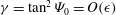 ${\it\gamma}=\tan ^{2}{\it\Psi}_{0}=O({\it\epsilon})$
. It is recognized that the solution (4.13) is unphysical in the case of a finite angle
${\it\gamma}=\tan ^{2}{\it\Psi}_{0}=O({\it\epsilon})$
. It is recognized that the solution (4.13) is unphysical in the case of a finite angle
 ${\it\Psi}_{0}\neq 0$
. While (4.13) is an exact solution to the KP equation (4.12), the breadth of the wave profile depends on the propagation direction,
${\it\Psi}_{0}\neq 0$
. While (4.13) is an exact solution to the KP equation (4.12), the breadth of the wave profile depends on the propagation direction,
 ${\it\Psi}_{0}$
. More precisely, the width of the soliton artificially changes by rotating the coordinate system. To correct this artefact, a heuristic fix is proposed by defining a new amplitude parameter
${\it\Psi}_{0}$
. More precisely, the width of the soliton artificially changes by rotating the coordinate system. To correct this artefact, a heuristic fix is proposed by defining a new amplitude parameter
 $\hat{a}_{0}=\tilde{a}_{0}/\cos ^{2}{\it\psi}=\tilde{a}_{0}(1+\tan ^{2}{\it\psi})=\tilde{a}_{0}(1+O({\it\varepsilon}))$
. Using this re-defined amplitude
$\hat{a}_{0}=\tilde{a}_{0}/\cos ^{2}{\it\psi}=\tilde{a}_{0}(1+\tan ^{2}{\it\psi})=\tilde{a}_{0}(1+O({\it\varepsilon}))$
. Using this re-defined amplitude
 $\hat{a}_{0}$
, (4.13) can be reduced to the KdV soliton:
$\hat{a}_{0}$
, (4.13) can be reduced to the KdV soliton:
 $$\begin{eqnarray}\tilde{{\it\eta}}\simeq \hat{a}_{0}\;\text{sech}^{2}\sqrt{\frac{3\hat{a}_{0}}{4\tilde{h}_{0}^{3}}}\left[\,\tilde{{\it\chi}}-\tilde{c}_{0}\left(1+\frac{\hat{a}_{0}}{2\tilde{h}_{0}}\right)\,\tilde{t}\,\right]+O({\it\varepsilon}^{2}).\end{eqnarray}$$
It is remarked that this heuristic modification makes the solution no longer exact to the KP equation (4.12). With the newly defined wave amplitude
 $\hat{a}_{0}$
, Miles’s parameter (4.2) is modified for a finite-but-small value of
$\hat{a}_{0}$
, Miles’s parameter (4.2) is modified for a finite-but-small value of
 ${\it\Psi}_{0}$
as
${\it\Psi}_{0}$
as
 $$\begin{eqnarray}k=\frac{\tan {\it\Psi}_{0}}{\sqrt{3a_{0}}\cos {\it\Psi}_{0}}.\end{eqnarray}$$
Comparing this with (4.8), we have
 $$\begin{eqnarray}a_{0}=\frac{2}{3}\frac{A_{0}}{\cos ^{2}{\it\Psi}_{0}}+O({\it\epsilon}^{2}).\end{eqnarray}$$
This relation between the physical wave amplitude and the KP wave amplitude gives the higher-order correction to the quasi-two-dimensional approximation, as will be shown in (5.14). In the next section, we show how it can be formally corrected using a normal form theory concerning the higher-order correction to the KP equation.
5 Normal form for the KP equation with higher-order corrections
We now construct a normal form of the KP equation with the higher-order corrections given by (2.9). The basic idea of the normal form theory has been presented by Kodama (Reference Kodama1985, Reference Kodama1987), Kodama & Mikhailov (Reference Kodama and Mikhailov1996) and Hiraoka & Kodama (Reference Hiraoka and Kodama2009). The goal of this section is to show that solutions of the normal form can be used to describe the Mach reflection even under the condition with a not-so-small finite value of
 ${\it\Psi}_{0}$
. The normal form theory also provides the next-order correction to the approximation of weak nonlinearity.
${\it\Psi}_{0}$
. The normal form theory also provides the next-order correction to the approximation of weak nonlinearity.
5.1 The normal form for the KdV equation
Before discussing a normal form for (2.9), we give a brief summary of the result for the case of the KdV equation. Taking
 $\partial _{Y}u=0$
in (2.12), we have the KdV equation with higher-order corrections:
$\partial _{Y}u=0$
in (2.12), we have the KdV equation with higher-order corrections:
 $$\begin{eqnarray}-4u_{t}=6uu_{x}+u_{xxx}+\left({\textstyle \frac{19}{60}}u_{xxxxx}+{\textstyle \frac{5}{3}}uu_{xxx}+{\textstyle \frac{53}{6}}u_{x}u_{xx}\right)+O({\it\epsilon}^{9/2}).\end{eqnarray}$$
(As stated earlier, the lower case letters
 $(x,y,z)$
are used instead of
$(x,y,z)$
are used instead of
 $(X,Y,T)$
for succinct expression.) According to Kodama (Reference Kodama1985), one can transform (5.1) with a formal change of variable,
$(X,Y,T)$
for succinct expression.) According to Kodama (Reference Kodama1985), one can transform (5.1) with a formal change of variable,
 $$\begin{eqnarray}u=U+\left(U_{xx}+{\textstyle \frac{4}{3}}U^{2}+{\textstyle \frac{1}{2}}U_{x}D^{-1}U\right)+O({\it\epsilon}^{3}),\end{eqnarray}$$
into the equation which we refer to as the normal form of (5.1):
 $$\begin{eqnarray}-4U_{t}=6UU_{x}+U_{xxx}+{\textstyle \frac{19}{60}}(U_{xxxxx}+10UU_{xxx}+20U_{x}U_{xx}+30U^{2}U_{x})+O({\it\epsilon}^{9/2}).\end{eqnarray}$$
Note that the higher-order term of
 $O({\it\epsilon}^{7/2})$
in this equation is the fifth-order symmetry of the KdV equation, and hence the normal form is integrable up to
$O({\it\epsilon}^{7/2})$
in this equation is the fifth-order symmetry of the KdV equation, and hence the normal form is integrable up to
 $O({\it\epsilon}^{7/2})$
. That is, we have an integrability not only at the KdV of
$O({\it\epsilon}^{7/2})$
. That is, we have an integrability not only at the KdV of
 $O({\it\epsilon}^{5/2})$
but also at the next-order correction of
$O({\it\epsilon}^{5/2})$
but also at the next-order correction of
 $O({\it\epsilon}^{7/2})$
. This means that the solitary waves are robust and their interaction properties remain the same as the KdV solitons even including the next-order correction.
$O({\it\epsilon}^{7/2})$
. This means that the solitary waves are robust and their interaction properties remain the same as the KdV solitons even including the next-order correction.
This is true even for the general form of the higher-order correction,
 $$\begin{eqnarray}{\it\alpha}_{1}u_{xxxxx}+{\it\alpha}_{2}uu_{xxx}+{\it\alpha}_{3}u_{x}u_{xx}+{\it\alpha}_{4}u^{2}u_{x},\end{eqnarray}$$
with arbitrary coefficients
 ${\it\alpha}_{1},\ldots ,{\it\alpha}_{4}$
. This implies that any weakly nonlinear long-wave equation whose leading order is approximated by the KdV equation is asymptotically integrable up to the next-order approximation. Then, using the transformation (5.2), one can find higher-order corrections of the KdV solitons including the phase shifts due to the soliton interactions (see Hiraoka & Kodama Reference Hiraoka and Kodama2009).
${\it\alpha}_{1},\ldots ,{\it\alpha}_{4}$
. This implies that any weakly nonlinear long-wave equation whose leading order is approximated by the KdV equation is asymptotically integrable up to the next-order approximation. Then, using the transformation (5.2), one can find higher-order corrections of the KdV solitons including the phase shifts due to the soliton interactions (see Hiraoka & Kodama Reference Hiraoka and Kodama2009).
Note that the normal form up to
 $O({\it\epsilon}^{7/2})$
admits a one-soliton solution in the form,
$O({\it\epsilon}^{7/2})$
admits a one-soliton solution in the form,
 $$\begin{eqnarray}U=A_{0}\,\text{sech}^{2}\sqrt{\frac{A_{0}}{2}}(x+x_{0}(t)),\end{eqnarray}$$
where
 $x_{0}(t)$
is determined by
$x_{0}(t)$
is determined by
 $(\text{d}x_{0}/\text{d}t):=(1/2)A_{0}+(19/60)A_{0}^{2}+O({\it\epsilon}^{3})$
. Then the solution of the higher-order KdV equation (5.1) is given by the transformation (5.2):
$(\text{d}x_{0}/\text{d}t):=(1/2)A_{0}+(19/60)A_{0}^{2}+O({\it\epsilon}^{3})$
. Then the solution of the higher-order KdV equation (5.1) is given by the transformation (5.2):
 $$\begin{eqnarray}u=A_{0}S^{2}+(A_{0}^{2}S^{2}-{\textstyle \frac{2}{3}}A_{0}^{2}S^{4})+O({\it\epsilon}^{3}),\end{eqnarray}$$
where
 $S:=\,\text{sech}\sqrt{A_{0}/2}(x+x_{0})$
. Note that the water surface
$S:=\,\text{sech}\sqrt{A_{0}/2}(x+x_{0})$
. Note that the water surface
 ${\it\eta}$
of (2.10) for the KdV case is given by
${\it\eta}$
of (2.10) for the KdV case is given by
 $$\begin{eqnarray}\displaystyle {\it\alpha}{\it\eta}={\textstyle \frac{2}{3}}A_{0}S^{2}+{\textstyle \frac{2}{9}}A_{0}^{2}S^{2}+{\textstyle \frac{1}{3}}A_{0}^{2}S^{4}+O({\it\epsilon}^{3}). & & \displaystyle\end{eqnarray}$$
This formula is consistent with the one obtained by Grimshaw (Reference Grimshaw1971), who derived the correction up to the third order.
5.2 Normal form of the KP equation
Now we define a normal form of (2.12) using the following transformation,
 $$\begin{eqnarray}u=U+({\it\beta}_{1}U_{xx}+{\it\beta}_{2}U^{2}+{\it\beta}_{3}U_{x}D^{-1}U+{\it\beta}_{4}D^{-2}U_{yy})+O({\it\epsilon}^{3}),\end{eqnarray}$$
where the
 ${\it\beta}_{j}$
values are determined in such a way that the transformed equation (normal form) has a ‘good’ property. First, we require that the normal form is reduced to the KdV normal form when we have
${\it\beta}_{j}$
values are determined in such a way that the transformed equation (normal form) has a ‘good’ property. First, we require that the normal form is reduced to the KdV normal form when we have
 $\partial _{y}u=0$
. That is, from (5.2), we have
$\partial _{y}u=0$
. That is, from (5.2), we have
 ${\it\beta}_{1}=1,{\it\beta}_{2}=(4/3),{\it\beta}_{3}=(1/2)$
, but
${\it\beta}_{1}=1,{\it\beta}_{2}=(4/3),{\it\beta}_{3}=(1/2)$
, but
 ${\it\beta}_{4}$
remains undetermined. Then we require that the normal form admits a solitary wave in the form of one-soliton solution,
${\it\beta}_{4}$
remains undetermined. Then we require that the normal form admits a solitary wave in the form of one-soliton solution,
 $$\begin{eqnarray}U=A_{0}\,\text{sech}^{2}\sqrt{\frac{A_{0}}{2}}(x+x_{0}(y,t)).\end{eqnarray}$$
This determines uniquely
 ${\it\beta}_{4}=1/2$
and the normal form of (2.12) is now given by
${\it\beta}_{4}=1/2$
and the normal form of (2.12) is now given by
 $$\begin{eqnarray}\displaystyle -4U_{t} & = & \displaystyle 6UU_{x}+U_{xxx}+3D^{-1}U_{yy}\nonumber\\ \displaystyle & & \displaystyle +\,{\textstyle \frac{19}{60}}(U_{xxxxx}+10UU_{xxx}+20U_{x}U_{xx}+30U^{2}U_{x})+{\textstyle \frac{3}{2}}U_{xyy}-{\textstyle \frac{3}{4}}D^{-3}U_{yyyy}\nonumber\\ \displaystyle & & \displaystyle -\,UD^{-1}U_{yy}+7U_{y}D^{-1}U_{y}+{\textstyle \frac{1}{4}}D^{-1}(U^{2})_{yy}+{\textstyle \frac{5}{2}}U_{x}D^{-2}U_{yy}+O({\it\epsilon}^{9/2}).\end{eqnarray}$$
The phase
 $x_{0}(y,t)$
satisfies
$x_{0}(y,t)$
satisfies
 $$\begin{eqnarray}-4\frac{\partial x_{0}}{\partial t}=2A_{0}+3\left(\frac{\partial x_{0}}{\partial y}\right)^{2}+\frac{19}{15}A_{0}^{2}+3A_{0}\left(\frac{\partial x_{0}}{\partial y}\right)^{2}-\frac{3}{4}\left(\frac{\partial x_{0}}{\partial y}\right)^{4}+O({\it\epsilon}^{3}).\end{eqnarray}$$
Setting the angle
 ${\it\Psi}_{0}$
of the soliton with
${\it\Psi}_{0}$
of the soliton with
 $(\partial x_{0}/\partial y)=\tan {\it\Psi}_{0}$
, we have the velocity
$(\partial x_{0}/\partial y)=\tan {\it\Psi}_{0}$
, we have the velocity
 $(\partial x_{0}/\partial t)$
of the KP soliton with the higher-order corrections. The corresponding solitary wave solution
$(\partial x_{0}/\partial t)$
of the KP soliton with the higher-order corrections. The corresponding solitary wave solution
 $u$
is then given by
$u$
is then given by
 $$\begin{eqnarray}u=A_{0}S^{2}+(A_{0}^{2}S^{2}+{\textstyle \frac{1}{2}}A_{0}\tan ^{2}{\it\Psi}_{0}S^{2}-{\textstyle \frac{2}{3}}A_{0}^{2}S^{4})+O({\it\epsilon}^{3}),\end{eqnarray}$$
and the water surface
 ${\it\eta}$
of (2.10) is given by
${\it\eta}$
of (2.10) is given by
 $$\begin{eqnarray}\displaystyle {\it\alpha}{\it\eta} & = & \displaystyle {\textstyle \frac{2}{3}}A_{0}S^{2}+{\textstyle \frac{2}{3}}\tan ^{2}{\it\Psi}_{0}S^{2}+{\textstyle \frac{2}{9}}A_{0}^{2}S^{2}+{\textstyle \frac{1}{3}}A_{0}^{2}S^{4}+O({\it\epsilon}^{3})\nonumber\\ \displaystyle & = & \displaystyle {\textstyle \frac{2}{3}}[A_{0}]S^{2}+{\textstyle \frac{2}{9}}[A_{0}]^{2}S^{2}+{\textstyle \frac{1}{3}}[A_{0}]^{2}S^{4}+O({\it\epsilon}^{3}),\end{eqnarray}$$
where
 $[A_{0}]:=A_{0}(1+\tan ^{2}{\it\Psi}_{0})=A_{0}/\cos ^{2}{\it\Psi}_{0}$
(see § 4.3). It is interesting to note that the correction to the quasi-two-dimensional approximation is entirely absorbed into the amplitude of the KdV equation (cf. (5.7)). This formula gives the relation between the observed amplitude
$[A_{0}]:=A_{0}(1+\tan ^{2}{\it\Psi}_{0})=A_{0}/\cos ^{2}{\it\Psi}_{0}$
(see § 4.3). It is interesting to note that the correction to the quasi-two-dimensional approximation is entirely absorbed into the amplitude of the KdV equation (cf. (5.7)). This formula gives the relation between the observed amplitude
 $a_{0}$
from numerical or laboratory experiments of a shallow-water wave system and the KP amplitude
$a_{0}$
from numerical or laboratory experiments of a shallow-water wave system and the KP amplitude
 $A_{0}$
. More explicitly, the observed amplitude
$A_{0}$
. More explicitly, the observed amplitude
 $a_{0}$
of one soliton up to
$a_{0}$
of one soliton up to
 $O({\it\epsilon}^{2})$
is given by
$O({\it\epsilon}^{2})$
is given by
 $$\begin{eqnarray}a_{0}=\frac{2}{3}[A_{0}]+\frac{5}{9}[A_{0}]^{2}\quad \text{ which gives }A_{0}=\frac{3a_{0}\cos ^{2}{\it\Psi}_{0}}{1+\sqrt{1+5a_{0}}}.\end{eqnarray}$$
This is a key equation when we apply the KP theory to laboratory experiments of shallow-water waves with finite values of
 ${\it\Psi}_{0}$
and
${\it\Psi}_{0}$
and
 $a_{0}$
.
$a_{0}$
.
5.3 Re-evaluation of the previous results based on the normal form
Recall that the KP equation is derived under the assumptions of quasi-two-dimensionality, weak dispersion and weak nonlinearity. Here, we show that it is necessary to include a higher-order correction for physical applications of the KP theory. Specifically, the observed wave amplitude in the laboratory and numerical experiments should be converted to the corresponding KP amplitude via the formula (5.14) that was derived from the normal form of the higher-order KP equation (5.10). Then, the KP parameter
 $k$
of (4.8) can be expressed in terms of the observed incident-wave amplitude
$k$
of (4.8) can be expressed in terms of the observed incident-wave amplitude
 $a_{0}$
and the incident angle
$a_{0}$
and the incident angle
 ${\it\Psi}_{0}$
by
${\it\Psi}_{0}$
by
 $$\begin{eqnarray}k=\frac{\tan {\it\Psi}_{0}}{\sqrt{2A_{0}}}=\frac{\sqrt{1+\sqrt{1+5a_{0}}}\tan {\it\Psi}_{0}}{\sqrt{6a_{0}}\cos {\it\Psi}_{0}}.\end{eqnarray}$$
Note that, for small
 $a_{0}$
, the KP parameter
$a_{0}$
, the KP parameter
 $k$
, including the higher-order corrections, reduces to the heuristically derived parameter in (4.15). The maximum wave amplification
$k$
, including the higher-order corrections, reduces to the heuristically derived parameter in (4.15). The maximum wave amplification
 $\hat{{\it\alpha}}$
in the KP theory can be obtained as follows.
$\hat{{\it\alpha}}$
in the KP theory can be obtained as follows.
For the case with
 $k<1$
(the Mach reflection), we have
$k<1$
(the Mach reflection), we have
 $$\begin{eqnarray}\hat{{\it\alpha}}=\frac{A_{[1,4]}}{A_{0}}=\frac{{\it\alpha}_{w}(1+\sqrt{1+5a_{0}})}{(1+\sqrt{1+5{\it\alpha}_{w}a_{0}})\cos ^{2}{\it\Psi}_{0}},\end{eqnarray}$$
where we have used (5.14) to evaluate the stem wave amplitudes
 $A_{[1,4]}$
and the incident wave amplitude
$A_{[1,4]}$
and the incident wave amplitude
 $A_{0}=A_{[1,3]}=A_{[2,4]}$
. It is emphasized that (5.16) shows the relation between the physical wave amplification
$A_{0}=A_{[1,3]}=A_{[2,4]}$
. It is emphasized that (5.16) shows the relation between the physical wave amplification
 ${\it\alpha}_{w}$
and the KP amplification
${\it\alpha}_{w}$
and the KP amplification
 $\hat{{\it\alpha}}$
.
$\hat{{\it\alpha}}$
.
For the case
 $k>1$
(regular reflection), we use the same formula in (4.1) with (5.15) which gives
$k>1$
(regular reflection), we use the same formula in (4.1) with (5.15) which gives
 $$\begin{eqnarray}\displaystyle \hat{{\it\alpha}} & = & \displaystyle \frac{4}{1+\sqrt{1-k^{-2}}}\approx 2\left(1+\frac{1}{4k^{2}}\right)=2\left(1+\frac{3a_{0}\cos ^{2}{\it\Psi}_{0}}{2(1+\sqrt{1+5a_{0}})\tan ^{2}{\it\Psi}_{0}}\right)\nonumber\\ \displaystyle & {\approx} & \displaystyle 2+\frac{3a_{0}(1-\sin ^{2}{\it\Psi}_{0})^{2}}{2\sin ^{2}{\it\Psi}_{0}}=2+a_{0}\left(\frac{3}{2\sin ^{2}{\it\Psi}_{0}}-3+\frac{3}{2}\sin ^{2}{\it\Psi}_{0}\right).\end{eqnarray}$$
Note here that the difference between (4.3) and this formula is
 $(1/2)\sin ^{2}{\it\Psi}_{0}$
, which is negligible for this approximation.
$(1/2)\sin ^{2}{\it\Psi}_{0}$
, which is negligible for this approximation.
The numerical and laboratory results are now re-evaluated with the new formulae (5.16) and (5.17) with (5.15), and the results are shown in figure 9(b). For comparison, the original prediction of Miles is also shown in figure 9(a). Laboratory data by Perroud (Reference Perroud1957) and Melville (Reference Melville1980) are not presented here because the propagation distance in their experiments was too short to achieve the asymptotic state.
Since the numerical simulations of Funakoshi (Reference Funakoshi1980) were conducted with small incident waves (
 $a_{0}=0.05$
), his results match the KP predictions very well; the slightly shifted deviation to the left in
$a_{0}=0.05$
), his results match the KP predictions very well; the slightly shifted deviation to the left in
 $k$
with the original Miles’s theory (figure 9
a) is now corrected. Tanaka (Reference Tanaka1993)’s results also match the theory; the higher-order correction substantially shifts his numerical data to the positive
$k$
with the original Miles’s theory (figure 9
a) is now corrected. Tanaka (Reference Tanaka1993)’s results also match the theory; the higher-order correction substantially shifts his numerical data to the positive
 $k$
value. Note that Tanaka’s numerical experiments were undertaken with a relatively large value of
$k$
value. Note that Tanaka’s numerical experiments were undertaken with a relatively large value of
 $a_{0}$
and a large value of the incidence angle
$a_{0}$
and a large value of the incidence angle
 ${\it\Psi}_{0}$
. The higher-order correction of the amplification factors (5.16) and (5.17) is very effective, although the agreement of Tanaka’s results with the KP theory is not as good as Funakoshi’s, especially for the data near
${\it\Psi}_{0}$
. The higher-order correction of the amplification factors (5.16) and (5.17) is very effective, although the agreement of Tanaka’s results with the KP theory is not as good as Funakoshi’s, especially for the data near
 $k=1$
. This is because the KP theory, even at higher order, still assumes small values of
$k=1$
. This is because the KP theory, even at higher order, still assumes small values of
 $a_{0}$
and
$a_{0}$
and
 $\tan {\it\Psi}_{0}$
. (Recall that Tanaka’s results were with
$\tan {\it\Psi}_{0}$
. (Recall that Tanaka’s results were with
 $a_{0}=0.3$
and
$a_{0}=0.3$
and
 ${\it\Psi}_{0}\approx 1$
near
${\it\Psi}_{0}\approx 1$
near
 $k=1$
.)
$k=1$
.)
As shown in figure 9, the higher-order KP theory results in a striking improvement in agreement of the laboratory data with the theory. While the laboratory data with the different incident wave angles appear in the separate datasets in the plot with Miles’s
 $k$
(in figure 9
a), the plot of the same datasets with the higher-order KP theory (figure 9
b) emerges as a single coherent dataset. In particular, the data with
$k$
(in figure 9
a), the plot of the same datasets with the higher-order KP theory (figure 9
b) emerges as a single coherent dataset. In particular, the data with
 ${\it\Psi}_{0}=0.35$
rad exhibit substantial improvement in the amplification factor.
${\it\Psi}_{0}=0.35$
rad exhibit substantial improvement in the amplification factor.
To obtain the maximum amplification near
 $k\approx 1$
, Tanaka (Reference Tanaka1993) used the incident wave amplitude
$k\approx 1$
, Tanaka (Reference Tanaka1993) used the incident wave amplitude
 $a_{0}=0.3$
in his numerical experiments and our laboratory experiments used the amplitude
$a_{0}=0.3$
in his numerical experiments and our laboratory experiments used the amplitude
 $a_{0}=0.277$
. The resulting amplifications for both numerical and laboratory results are
$a_{0}=0.277$
. The resulting amplifications for both numerical and laboratory results are
 $\hat{{\it\alpha}}\approx 3$
. Because the wave amplitude along the wall is close to unity (
$\hat{{\it\alpha}}\approx 3$
. Because the wave amplitude along the wall is close to unity (
 $\neq O({\it\varepsilon})$
), such not-so-small finite-amplitude conditions clearly violate the assumption of weak nonlinearity. Nonetheless, all of the numerical and laboratory data shown in figure 9 are in good agreement with the higher-order KP theory. In spite of the violations of the small parameters
$\neq O({\it\varepsilon})$
), such not-so-small finite-amplitude conditions clearly violate the assumption of weak nonlinearity. Nonetheless, all of the numerical and laboratory data shown in figure 9 are in good agreement with the higher-order KP theory. In spite of the violations of the small parameters
 $a_{0}$
and
$a_{0}$
and
 ${\it\Psi}_{0}$
, this rather unexpected performance of the theory is remarkable.
${\it\Psi}_{0}$
, this rather unexpected performance of the theory is remarkable.

Figure 9. Numerical and experimental results of (a) the amplification factor
 ${\it\alpha}_{w}$
versus
${\it\alpha}_{w}$
versus
 $k$
, the Miles parameter (4.2) and (b) the KP amplification factor
$k$
, the Miles parameter (4.2) and (b) the KP amplification factor
 $\hat{{\it\alpha}}$
versus the new higher-order KP parameter (5.15). The crosses
$\hat{{\it\alpha}}$
versus the new higher-order KP parameter (5.15). The crosses
 $\times$
show the numerical results by Funakoshi (Reference Funakoshi1980), the hollow triangles ▵ show the numerical results by Tanaka (Reference Tanaka1993), the solid circles ● are the laboratory data by Li et al. (Reference Li, Yeh and Kodama2011) with
$\times$
show the numerical results by Funakoshi (Reference Funakoshi1980), the hollow triangles ▵ show the numerical results by Tanaka (Reference Tanaka1993), the solid circles ● are the laboratory data by Li et al. (Reference Li, Yeh and Kodama2011) with
 ${\it\Psi}_{0}=0.35$
rad, solid triangles ▴ with
${\it\Psi}_{0}=0.35$
rad, solid triangles ▴ with
 ${\it\Psi}_{0}=0.52$
rad and solid squares ▪ with
${\it\Psi}_{0}=0.52$
rad and solid squares ▪ with
 ${\it\Psi}_{0}=0.70$
rad.
${\it\Psi}_{0}=0.70$
rad.
6 Summary and conclusion
We first reviewed a solution methodology for the KP equation that was established by one of the present authors and his colleagues (e.g. Chakravarty & Kodama Reference Chakravarty and Kodama2009; Kodama et al. Reference Kodama, Oikawa and Tsuji2009; Kodama Reference Kodama2010). The exact solutions, called KP solitons, are presented. The (2,2)-soliton solutions are considered, which can be classified to seven types and each of them is effectively represented by the corresponding chord diagram (figure 2). Among them, the (3412)-type and the (2143)-type forming an ‘X-shaped’ wave pattern are analysed. It is shown that those two types are realized quantitatively in the laboratory environment.
We then examine the generation processes of the (2,2)-soliton solutions from the initial state of a single soliton obliquely incident onto a perfectly reflective wall. This creates a symmetrical pattern (or mirror image) about the wall, and the asymptotic state of the KP theory is the (3412)-type or the (2143)-type. It is shown that the critical condition of the 4-fold amplification predicted by Miles (Reference Miles1977b
) can be interpreted from the chord diagram at the confluent state of the (3412)-type and the (2143)-type (figure 7). This theoretical prediction of the amplification was not verified previously in the physical domain, partly because the process to reach its asymptotic state takes a long time in the laboratory and numerical experiments, and more importantly the assumption of ‘small’ wave incident angle
 ${\it\Psi}_{0}$
is sensitive and difficult to realize in the physical domain. To remedy these shortcomings, we extend the KP theory to include a higher-order correction with the use of normal form theory. It is demonstrated that the higher-order theory is capable of predicting accurately the Mach reflection phenomenon resulting from the laboratory and numerical experiments; therefore, the critical 4-fold amplification of two oblique solitons interacting is now likely accepted to be reality.
${\it\Psi}_{0}$
is sensitive and difficult to realize in the physical domain. To remedy these shortcomings, we extend the KP theory to include a higher-order correction with the use of normal form theory. It is demonstrated that the higher-order theory is capable of predicting accurately the Mach reflection phenomenon resulting from the laboratory and numerical experiments; therefore, the critical 4-fold amplification of two oblique solitons interacting is now likely accepted to be reality.
Acknowledgements
We are grateful to Dr Jia and Dr Li for their help in the preliminary analysis. Y.K. was partially supported by NSF grant DMS-1410267; H.Y. was partially supported by Oregon Sea grant Program (NA06OAR4170010-NB154L and NA10OAR4170059-NA223L) and the Oregon State University Edwards Endowment.


