


1. Introduction
The present-day third-generation spectral wave models generally solve the action balance equation (e.g. Komen et al. Reference Komen, Cavaleri, Donelan, Hasselmann, Hasselmann and Janssen1994; Janssen Reference Janssen2008) to predict the evolution of ocean surface waves:
 \begin{equation} \frac{\mathrm{d} N}{\mathrm{d}t} = \frac{S_{in} +S_{ds} + S_{nl} + \cdots}{\omega}, \end{equation}
where  $N(k, \theta; \boldsymbol {x}, t) = F(k, \theta; \boldsymbol {x}, t) / \omega$ is the wave action density spectrum,
  $\omega$ is the intrinsic (radian) frequency,
  $k = |\boldsymbol {k}|$ is the wavenumber and
  $\theta$ is the propagation direction of wave energy. For deep-water waves,
  $\omega$ and
  $k$ are linked through the linear dispersion relation
 \begin{equation} \omega^2 = g k, \end{equation}
where  $g$ is the gravitational acceleration. The right-hand side of (1.1) consists of sources and sinks of wave energy, including wind input
  $S_{in}$, wave breaking-induced dissipation
  $S_{ds}$ and nonlinear four-wave interaction
  $S_{nl}$ (e.g. Cavaleri et al. Reference Cavaleri2007, Reference Cavaleri2018). Among these various physical processes,
  $S_{nl}$ is known to play a central role in the development of wind-generated wave spectrum through controlling the downshifting of the spectral peak, the angular spreading and the high-frequency spectral tail (Hasselmann et al. Reference Hasselmann1973; Young & van Vledder Reference Young and van Vledder1993; Badulin et al. Reference Badulin, Pushkarev, Resio and Zakharov2005, Reference Badulin, Babanin, Zakharov and Resio2007).
The mathematical formulation of the nonlinear transfer  $S_{nl}$ for a continuous wave spectrum that describes how wave energy is redistributed over the spectral space due to resonant four-wave interactions was first established by Hasselmann (Reference Hasselmann1962):
 \begin{gather} \frac{\mathrm{d} C_1}{\mathrm{d} t} = 4 {\rm \pi}\int \left[ T^2_{1, 2, 3, 4} \mathcal{F}_{1,2,3,4} \delta (\Delta \boldsymbol{k}) \delta(\Delta \omega) \right]\,\mathrm{d}\boldsymbol{k_{2, 3, 4}} , \end{gather}
 \begin{gather}\mathcal{F}_{1, 2, 3, 4} = C_3 C_4 (C_1 + C_2) - C_1 C_2 (C_3 + C_4) , \end{gather}
where  $C_1 = C(\boldsymbol {k_1}) = g N(k, \theta ) / k$ is the action spectrum,
  $T_{1, 2, 3, 4} = T(\boldsymbol {k_1}, \boldsymbol {k_2}, \boldsymbol {k_3}, \boldsymbol {k_4})$ is the interaction coefficient (Krasitskii Reference Krasitskii1994; Janssen Reference Janssen2009),
  $\Delta \boldsymbol {k} = \boldsymbol {k_1} + \boldsymbol {k_2} - \boldsymbol {k_3} - \boldsymbol {k_4}$ and
  $\Delta \omega = \omega _1 + \omega _2- \omega _3 - \omega _4$ are wavenumber and frequency mismatch and
  $\mathrm {d} \boldsymbol {k_{2,3,4}} = \mathrm {d} \boldsymbol {k_2}\, \mathrm {d} \boldsymbol {k_3}\, \mathrm {d} \boldsymbol {k_4}$. The two
  $\delta$-functions in (1.3) dictate that only four resonant wave components satisfying
 \begin{equation} \left. \begin{gathered} \boldsymbol{k_1} + \boldsymbol{k_2} = \boldsymbol{k_3} + \boldsymbol{k_4},\\ \omega_1 + \omega_2 = \omega_3 + \omega_4, \end{gathered} \right\} \end{equation}
could exchange energy and momentum. The Hasselmann equation (1.3) is also known as the standard kinetic equation and Boltzmann integral for a homogeneous, quasi-Gaussian wave field. Hereafter, we refer to it as the Hasselmann kinetic equation (HKE). According to (1.1) and (1.3), we have
 \begin{equation} S_{nl}(k, \theta) = \omega \left.\frac{\mathrm{d} N}{\mathrm{d}t} \right\rvert_{nl} = \frac{\omega k}{g} \frac{\mathrm{d} C_1}{\mathrm{d} t}. \end{equation}
An important hypothesis underpinning the derivation of the HKE is the action density  $C (\boldsymbol {k})$ evolves on a slow (‘kinetic’) time scale of
  $O(1 / \varepsilon ^{4} \omega _0)$, where
  $\varepsilon$ and
  $\omega _0$ are typical wave steepness and frequency of the wave field (Annenkov & Shrira Reference Annenkov and Shrira2006). Consequently, as a large-time limit, the HKE does not include contributions from non-resonant interactions (
 $\Delta \omega \neq 0$).
Realizing the possible importance of non-resonant four-wave interactions for spectral evolution on a fast time scale  $O(1 / \varepsilon ^{2} \omega _0)$, Janssen (Reference Janssen2003) proposed to modify the HKE as
 \begin{equation} \frac{\mathrm{d} C_1}{\mathrm{d} t} = 4 \int \left[ T^2_{1, 2, 3, 4} \mathcal{F}_{1,2,3,4} \delta (\Delta \boldsymbol{k}) R (\Delta \omega, t)\right]\,\mathrm{d} \boldsymbol{k_{2, 3, 4}}, \end{equation}
where
 \begin{equation} R (\Delta \omega, t) = {\textrm{Re}} \int_{0}^{t} \exp({\textrm{i}\Delta \omega (t - \tau)})\,\mathrm{d} \tau = \frac{\sin (\Delta \omega t)}{\Delta \omega}, \end{equation}
and
 \begin{equation} \left. \begin{gathered} \lim_{t \rightarrow 0} R(\Delta \omega, t) = t,\\ \lim_{t \rightarrow \infty} R(\Delta \omega, t) = {\rm \pi}\delta(\Delta \omega). \end{gathered} \right\} \end{equation}
From (1.9) we know that (i) for short times Janssen's kinetic equation (JKE) incorporates contributions from both resonant and non-resonant interactions, and (ii) the JKE is equivalent to the HKE for large times. In the context of a one-dimensional (1-D; unidirectional) wave spectrum, for which the HKE predicts no spectral change because of the non-existence of resonant quadruplets, Janssen (Reference Janssen2003) demonstrated that his JKE could capture remarkably well the spectral evolution as revealed by direct simulations based on the Zakharov equation (Zakharov Reference Zakharov1968).
It is noteworthy that the JKE still assumes the underlying action density  $C(\boldsymbol {k})$ itself and, therefore, the action density product terms
  $\mathcal {F}_{1,2,3,4}$ (1.4) are slowly varying (i.e. quasi-stationary). Annenkov & Shrira (Reference Annenkov and Shrira2006) further extended this kinetic equation by fully discarding the quasi-stationarity assumption, resulting in the so-called generalized kinetic equation (GKE). Later, Gramstad & Stiassnie (Reference Gramstad and Stiassnie2013, hereafter GS13) advanced the GKE one-step further by taking into account high-order effects related to the Stokes correction of the frequencies. The authors, however, found the nonlinear Stokes correction not important for the cases they explored. Neglecting the effect of the Stokes-corrected frequencies, the GKE is formulated as (e.g. Reference Gramstad and StiassnieGS13):
 \begin{gather} \frac{\mathrm{d} C_1}{\mathrm{d} t} = 4 {\textrm{Re}} \int \left[T^2_{1, 2, 3, 4} \delta (\boldsymbol{\Delta k}) \exp({\textrm{i}\Delta \omega t}) I(t) \right]\,\mathrm{d} \boldsymbol{k_{2, 3, 4}}, \end{gather}
 \begin{gather}I(t) = \int_{0}^{t} \mathcal{F}_{1, 2, 3, 4} (\tau) \exp({-\textrm{i}\Delta \omega \tau })\, \mathrm{d} \tau. \end{gather}
Here we have implicitly assumed a Gaussian initial condition such that the fourth-order cumulant and, hence, the time integral  $I(t)$ are initially zero (see Reference Gramstad and StiassnieGS13 for more details). As summarized in table 1, the GKE not only includes the non-resonant interactions but also suggests the evolution of a wave field depends on its previous history of evolution (i.e. non-local in time; Annenkov & Shrira Reference Annenkov and Shrira2018, hereafter AS18). It is worth mentioning that the GKE will turn into the JKE if we take the action product term
  $\mathcal {F}_{1, 2, 3, 4}$ in (1.11) outside the time integral and then will naturally become the HKE if we further adopt the large time limit (1.9).
Table 1. Features included in different kinetic equations (nonlinear four-wave interaction transfer) for a homogenous, quasi-Gaussian wave field.

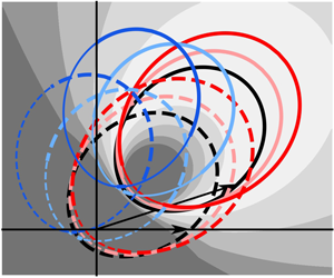
The difference in the interaction space for the HKE and JKE/GKE is visualized in figure 1. As constrained by (1.5), for  $\boldsymbol {k_1}$ and
  $\boldsymbol {k_3}$ fixed, the resonant
  $\boldsymbol {k_2}$ and
  $\boldsymbol {k_4}$ components will trace out two closed, ‘egg-shaped’ curves in wavenumber space (black lines in figure 1), which are referred to as loci in the literature (Webb Reference Webb1978; van Vledder Reference van Vledder2006). For the non-resonant quadruplets, which the JKE and GKE take into consideration but the HKE does not, there will be more numerous possible wavenumber configurations owing to the removal of the
  $\delta$-function over
  $\Delta \omega$. In essence, the non-resonant
  $\boldsymbol {k_2}$ component can be any non-zero point in the wavenumber plane which does not fall on the resonant locus. For illustration purposes only, we also show a few subsets of non-resonant quadruplets in figure 1. For example, if we have
  $\boldsymbol {k_{2, nr}} = \delta ^{i} \boldsymbol {k_{2, r}},\ i = 1, 2, \ldots$ and
  $\delta > 1$, where the subscripts ‘
 ${nr}$’ and ‘
 $r$’ denote non-resonant and resonant wave components, respectively, we obtain a family of newly formed, magnified loci for
  $\boldsymbol {k_{2, nr}}$ and accordingly
  $\boldsymbol {k_{4, nr}}$ (red lines in figure 1). Similarly, if we rotate the resonant
  $\boldsymbol {k_2}$ locus counterclockwise through an angle
  $\theta _j = j \Delta \theta ,\ j = 1, 2, \ldots$ about the origin, another set of loci for
  $\boldsymbol {k_{2, nr}}$ and
  $\boldsymbol {k_{4, nr}}$ will be acquired (blue lines in figure 1). In practice, however, only non-resonant quadruplets that are not far from resonance (i.e. quasi-resonant) are considered (see § 2 for further explanation).

Figure 1. Illustration of the difference in the interaction space for the HKE and JKE/GKE for a given combination of  $\boldsymbol {k_1}$ (0.1, 0) and
  $\boldsymbol {k_3}$ (0.15, 0.05) (adapted from figure 6 of van Vledder Reference van Vledder2006). The black solid (dashed) line presents the locus for the resonant
  $\boldsymbol {k_2}$ (
 $\boldsymbol {k_4}$) component, computed with the polar method of van Vledder (Reference van Vledder2000). Shaded contour: the normalized frequency mismatch
  $|\Delta \omega _n| = |\Delta \omega | / \min (\omega _1, \omega _2, \omega _3, \omega _4)$. Red lines
  $\delta _i$: the resonant
  $\boldsymbol {k_2}$ locus is magnified by
  $\delta ^{i}$ and
  $\delta = 1.1$, blue lines
  $\theta _j$: the resonant
  $\boldsymbol {k_2}$ locus is rotated counterclockwise through
  $\theta _j = 15^{\circ } j$ about the origin. The thick part of each coloured circle highlights the non-resonant quadruplets with
  $|\Delta \omega _n| \le 0.1$.
The first computation of two-dimensional (2-D) wave spectra with the GKE was performed by Reference Gramstad and StiassnieGS13. Gramstad & Babanin (Reference Gramstad and Babanin2016, hereafter GB16) further implemented their GKE algorithm in the spectral wave model WAVEWATCH III (hereafter WW3, version 3.14; Tolman Reference Tolman2009), and reported remarkable differences between the HKE and GKE simulations for both directionally narrow and broad spectra, and for spectra subject to sudden changes in wind speed or direction. These results, however, are inconsistent with a series of work by Annenkov & Shrira (Reference Annenkov and Shrira2015, Reference Annenkov and Shrira2016, Reference Annenkov and Shrira2018, Reference Annenkov and Shrira2019) who demonstrated that the GKE results are not significantly different from the HKE (in terms of spectral shape) even for steep, narrow-banded and directionally narrow wave fields. Therefore, it is still puzzling whether the quasi-resonant four-wave interactions and non-locality of  $C(\boldsymbol {k})$, as incorporated by the GKE, are critical for development of 2-D wave spectra.
Motivated by these disputes, we revisited the GKE algorithm developed by Reference Gramstad and BabaninGB16, rewrote it as a set of subroutines and then implemented them in WW3 (v6.07; WW3DG 2019). These efforts revealed that two numerical aspects pertaining to the discretization of the GKE and to the source term integration were not handled properly in Reference Gramstad and BabaninGB16. Corrections of these non-trivial numerical aspects are proposed in this study; meanwhile, considering the high similarity between the JKE and GKE, we implement the JKE under the framework of the GKE in WW3 as well (§ 2). Comparisons of three kinetic equations (HKE, JKE, GKE) are then carefully investigated through (i) a duration-limited wave growth test (§ 3), (ii) adiabatic evolution of a steep Gaussian wave spectrum (§ 4), (iii) response of ocean waves to turning winds (§ 5) and (iv) development of ice-coupled waves (§ 6). Note that following Young (Reference Young1999), the duration-limited wave growth here specifically refers to the case where the wave field is sufficiently distant from land boundaries and grows under a spatially homogeneous and stationary wind field (i.e. constant wind speed and direction). Other cases considered in the paper are still duration-limited (spatially homogeneous and no dependence on the spatial coordinate) but are subject to different external environmental forcing.
It is seen that good agreement with the findings of Annenkov & Shrira can be achieved with the updated GKE algorithm. As our GKE algorithm and that used by Annenkov & Shrira were developed fully independently, it appears reasonable to unambiguously conclude that beyond our expectation, corrections embraced in the present JKE/GKE relative to the HKE do not give rise to significantly different spectral evolution of directional wind waves, provided that wave spectra are fairly smooth (i.e. no strong perturbations) and the directionality is sufficiently broad. More detailed discussion and conclusions of these findings are given in §§ 7 and 8, respectively.
2. Numerical algorithm
2.1. The GKE
The GKE algorithm and its implementation in WW3, originally developed by Reference Gramstad and BabaninGB16, together with relevant updates, are documented in the following subsections, including the discretization of equations, quasi-resonant filter, phase mixing and source term integration.
2.1.1. Discretization
According to (1.10), the incremental change of action  $\delta C_1$ in an infinitesimal phase element
  $\delta \boldsymbol {k_1}$ and time interval
  $\Delta t$ is
 \begin{equation} \delta C_1 = \frac{\mathrm{d} C_1}{\mathrm{d} t} \delta \boldsymbol{k_1} \Delta t = 4 {\textrm{Re}} \int \left[ T^2_{1, 2, 3, 4} \delta (\Delta \boldsymbol{k}) \exp({\textrm{i}\Delta \omega t}) I(t) \right]\,\mathrm{d} \boldsymbol{k_{2, 3, 4}} \delta \boldsymbol{k_1} \Delta t, \end{equation}
and owing to the symmetry of four-wave interactions (Hasselmann & Hasselmann Reference Hasselmann and Hasselmann1985),
 \begin{equation} \delta C_1 = \delta C_2 = - \delta C_3 = -\delta C_4. \end{equation}
In this respect, Reference Gramstad and StiassnieGS13 and Janssen & Janssen (Reference Janssen and Janssen2019) reported that both the GKE and JKE conserve the total wave action, momentum and energy (see also Shrira & Annenkov Reference Shrira and Annenkov2013). Therefore, the principle of detailed balance (2.2) holds for these two equations, just as for the HKE. When implemented in WW3, (1.10) and (2.1) are discretized as
 \begin{equation} \frac{\mathrm{d} C_1}{\mathrm{d} t} = \left.\sum_{\boldsymbol{k_{2, 3, 4}}} \mathcal{M}_{1,2,3,4} \right/ \delta \boldsymbol{k_1}, \end{equation}
where  $\delta \boldsymbol {k}$ is the area of the given wavenumber bin and
 \begin{equation} \mathcal{M}_{1,2,3,4} = 4 T^2_{1, 2, 3, 4} \delta (\Delta \boldsymbol{k}) {\textrm{Re}} \left[ \exp({\textrm{i}\Delta \omega t}) I(t) \right] \delta \boldsymbol{k_{1, 2, 3, 4}}. \end{equation}
The time integral  $I(t)$ is solved iteratively by
 \begin{align} I (t) &= I (t - \Delta t) + \int_{t - \Delta t}^{t} \mathcal{F}_{1, 2, 3, 4} (\tau) \exp({-\textrm{i}\Delta \omega \tau })\,\mathrm{d} \tau, \nonumber\\ &= I (t - \Delta t) + \frac{\Delta t}{2} \left[ \mathcal{F}_{1, 2, 3, 4} (t - \Delta t) \exp({-\textrm{i}\Delta \omega (t - \Delta t) }) + \mathcal{F}_{1, 2, 3, 4} (t) \exp({-\textrm{i}\Delta \omega t }) \right]. \end{align}
For an intermediate step of estimating (2.3)–(2.5), Reference Gramstad and BabaninGB16 considered waves of different modes as discrete wave systems and have adopted
 \begin{equation} \sum_{\boldsymbol{k_{2, 3, 4}}} \mathcal{F}_{1, 2, 3, 4} \delta (\Delta \boldsymbol{k}) \delta \boldsymbol{k_{1, 2, 3, 4}} = \sum_{\boldsymbol{k_{2, 3, 4}}} C_3^{\prime} C_4^{\prime} (C_1^{\prime} + C_2^{\prime}) - C_{1}^{\prime} C_{2}^{\prime} (C_3^{\prime} + C_4^{\prime}), \end{equation}
where  $C^{\prime } (\boldsymbol {k}) = C(\boldsymbol {k}) \delta \boldsymbol {k}$. For discrete spectral wave models with a logarithmically spaced frequency grid, however, (2.6) should be more naturally solved by
 \begin{equation} \sum_{\boldsymbol{k_{2, 3, 4}}} \mathcal{F}_{1, 2, 3, 4} \delta (\Delta \boldsymbol{k}) \delta \boldsymbol{k_{1, 2, 3, 4}} = \sum_{\boldsymbol{k_{2, 3, 4}}} \mathcal{F}_{1, 2, 3, 4} \delta \boldsymbol{k_{1, 2, 3}}, \end{equation}
where the  $\delta$-function over wavenumber is eliminated because of
 \begin{equation} \int \delta (\Delta \boldsymbol{k})\,\mathrm{d} \boldsymbol{k_4} = \int \delta (\boldsymbol{k_1} + \boldsymbol{k_2} - \boldsymbol{k_3} - \boldsymbol{k_4})\,\mathrm{d} \boldsymbol{k_4} = 1 \end{equation}
according to Tracy & Resio (Reference Tracy and Resio1982). Clearly, for an equally spaced wavenumber grid, (2.6) and (2.7) are equivalent. More technical details for solving (2.3)–(2.7) are presented in appendix A.
2.1.2. Filtration of quadruplets
To reduce the computational expense of the GKE, we only consider wavenumber configurations satisfying
 \begin{equation} \left. \begin{gathered} \boldsymbol{k_1} + \boldsymbol{k_2} = \boldsymbol{k_3} + \boldsymbol{k_4},\\ |\Delta \omega| \leq \lambda_c \min (\omega_1, \omega_2, \omega_3, \omega_4), \end{gathered} \right\} \end{equation}
as valid quadruplets. Here  $\lambda _c$ is a cut-off factor used to filter out quartets very far from resonance which contribute little to spectral evolution (figure 1). From a theoretical point of view, Reference Gramstad and BabaninGB16 suggested
  $\lambda _c = O(\varepsilon ^{2})$ (note that in generic situations
  $\Delta \omega \sim O(\varepsilon ^2)$ (Annenkov & Shrira Reference Annenkov and Shrira2006)) and adopted
  $\lambda _c = 0.08$ for their simulations. Similarly, Reference Annenkov and ShriraAS18 pointed out that for short-term simulations (
 ${O}(10^2)$ wave periods),
  $\lambda _c$ of
  ${O}(10^{-2})$ is sufficient; instead, for better numerical stability a larger
  ${O}(10^{-1})$ value for
  $\lambda _c$ is preferred for long-term simulations (
 ${O}(10^3)$ periods).
For a given quadruplet, we choose  $\boldsymbol {k_1}$,
  $\boldsymbol {k_2}$ and
  $\boldsymbol {k_3}$ at the wavenumber grid points, and
  $\boldsymbol {k_4}$ is naturally determined by (2.9). Unless otherwise specified, the action density
  $C(\boldsymbol {k_4})$ is obtained through bilinear interpolation (van Vledder Reference van Vledder2006). When
  $\boldsymbol {k_4}$ falls beyond the spectral grid, we assume
 \begin{equation} C(k_4) = \begin{cases} 0 , & \text{for } k_4 < k_{min},\\ C(k_{max}) \left( \dfrac{k_4}{k_{max}} \right)^{n/2 - 2}, & \text{for } k_4 > k_{max},\end{cases} \end{equation}
where  $k_{min}$ and
  $k_{max}$ are the minimum and maximum wavenumbers within in the spectral grid, and
  $n=-5$ is the prescribed high-frequency power law for frequency spectrum (i.e.
  $E(\,f) \propto f^{n}$).
2.1.3. Phase mixing
As noted in § 1, the GKE (2.3)–(2.5) is generally solved by assuming wave phases are initially completely uncorrelated, i.e. a cold start with  $I(t=0) = 0$ (Reference Gramstad and StiassnieGS13; Reference Annenkov and ShriraAS18). As wave field evolves, the nonlinear four-wave interactions give rise to deviation from Gaussianity (Janssen Reference Janssen2003), resulting in non-zero fourth-order cumulant and, hence, non-zero
  $I(t)$. Some physical processes such as wave breaking (e.g. Babanin et al. Reference Babanin, Chalikov, Young and Savelyev2010) may uncorrelate phases (i.e. phase re-mixing) at certain times. Reference Gramstad and StiassnieGS13 and Reference Gramstad and BabaninGB16 suggested such effect could be incorporated in the GKE algorithm by restarting the GKE (setting
  $t=0$) every
  $N_{pm}$ characteristic wave periods (in terms of
  $T_{0, -1}$; appendix B) while keeping the action spectrum unchanged. As we show in the following, the phase re-mixing is also desired to suppress the numerical instability of the GKE for long-term simulations.
Two options for  $N_{pm}$ have been made available:
  $N_{pm}$ can either be a fixed constant (
 $N_{pm} \sim O (10^2)$) or explicitly depend on the dominant breaking probability
  $b_T$ by employing
  $N_{pm} = 1 / b_T$ and
 \begin{equation} b_T = 85.1 (\varepsilon_{p,w} - 0.055)^{2.33} \end{equation}
according to Babanin, Young & Banner (Reference Babanin, Young and Banner2001, their figure 12). Here  $\varepsilon _{p, w}$ is the significant steepness of the spectral peak:
 \begin{equation} \varepsilon_{p,w} = 2 \left[\int_{0.7\,f_{p,w}}^{1.3f_{p,w}} E_w(\,f) \,\mathrm{d}f \right]^{1/2} k_{p,w}, \end{equation}
where  $E_w(\,f)$ is the 1-D wave spectrum,
  $k_{p, w}$ and
  $f_{p, w}$ are the peak wavenumber and frequency, respectively. The subscript ‘
 $w$’ means these quantities are computed from wave spectrum
  $F(\,f, \theta )$ after filtration of swells. Following Bidlot (Reference Bidlot2001), we consider spectral components as wind seas if
 \begin{equation} \frac{c}{U_{10} \cos (\theta - \theta_u)} < \beta_w, \end{equation}
where  $c= \omega / k$ is the phase velocity,
  $U_{10}$ (
 $\theta _u$) is the wind velocity (direction) 10 m above the sea surface,
  $\beta _w$ is an empirical wind forcing parameter with
  $\beta _w \in [1.0, 2.0]$ used in the literature (e.g. Janssen et al. Reference Janssen, Lionello, Reistad and Hollingsworth1989; Barstow et al. Reference Barstow2005). Here, by default, we have chosen
  $\beta _w = 1.2$.
2.1.4. Source term integration
Third-generation spectral wave models usually employ a semi-implicit or implicit integration scheme to calculate the change of action density  $\Delta N$ in the time step
  $\Delta t$ from source terms
  $\mathcal {S} = S / \omega$:
 \begin{equation} \Delta N(k, \theta) = \frac{\mathcal{S} (k, \theta) \Delta t}{1 - \epsilon D(k, \theta) \Delta t}, \end{equation}
where  $D(k, \theta ) = \partial \mathcal {S} (k, \theta ) / \partial N(k, \theta )$ is the diagonal term and
  $\epsilon =1/2 \text { or } 1$ is the implicitness parameter (e.g. The WAMDI Group 1988; van Vledder Reference van Vledder2006; Tolman Reference Tolman2013). Owing to the presence of the time integral
  $I(t)$ in (1.10) which explicitly depends on the history of the evolution of wave spectrum (in terms of the action product term
  $\mathcal {F}_{1,2,3,4} (\tau )$), it is challenging, if not impossible, to compute the diagonal term
  $D(k, \theta )$ for the GKE. To circumvent this problem, we adopt the explicit dynamic time-stepping scheme (
 $\epsilon = 0$) of Tolman (Reference Tolman1992) for source term integration when
  $S_{nl}$ is based on the GKE.
For a fixed global time step  $\Delta t_g$, the source term integration is performed over a number of dynamic time steps
  $\Delta t_d^i$:
 \begin{equation} \left. \begin{gathered}
\Delta t_d^i = \min \left[ \Delta t_g - \sum_{j=1}^{i-1}
\Delta t_d^j, \quad \min_{ { \forall \theta; \, f \le \,
f_{hf}} } \left( \frac{\Delta N_{max}(k)}{ |\mathcal{S} (k,
\theta)|} \right)^i \right], \\ \Delta t_d^i = \max \left(
\Delta t_d^i, \, \Delta t_{d, min} \right) \quad \text{and}
\quad \sum \Delta t_d^i = \Delta t_g,
\end{gathered} \right\}
\end{equation}
\begin{equation} \left. \begin{gathered}
\Delta t_d^i = \min \left[ \Delta t_g - \sum_{j=1}^{i-1}
\Delta t_d^j, \quad \min_{ { \forall \theta; \, f \le \,
f_{hf}} } \left( \frac{\Delta N_{max}(k)}{ |\mathcal{S} (k,
\theta)|} \right)^i \right], \\ \Delta t_d^i = \max \left(
\Delta t_d^i, \, \Delta t_{d, min} \right) \quad \text{and}
\quad \sum \Delta t_d^i = \Delta t_g,
\end{gathered} \right\}
\end{equation}
where  $\Delta N_{max} (k)$ is the maximum allowed change of action density per spectral bin per time step that is generally chosen as a certain fraction (
 ${\sim }10\,\%$) of the Pierson–Moskowitz energy level,
  $\Delta t_{d, min}$ is a user-defined minimum dynamic time step, and
  $f_{hf} = N_{hf} / T_{0, -1}$ is the high-frequency limit of the prognostic region of the spectrum. The reader is referred to Tolman (Reference Tolman1992) and WW3DG19 for more technical details of this explicit dynamic scheme. Reference Gramstad and BabaninGB16 assumed
  $D(k, \theta ) = 0$ but used the default implicit scheme (
 $\epsilon =1$) in WW3. These two settings are apparently incompatible particularly when both
  $S_{nl}$ and other terms (e.g.
  $S_{in}$,
  $S_{ds}$) are activated in the computations.
2.2. The JKE and HKE
We implement the JKE (1.7) under the framework of the GKE algorithm similarly as mentioned previously except that  $R(\Delta \omega , t)$ is solved directly based on (1.8) and (1.9). Likewise, the phase mixing for the JKE is achieved by restarting it (setting
  $t=0$) periodically. The HKE (1.3) is computed based on the Webb–Resio–Tracy (WRT) approach (Webb Reference Webb1978; Tracy & Resio Reference Tracy and Resio1982; Resio & Perrie Reference Resio and Perrie1991; van Vledder Reference van Vledder2006) with an implicit (
 $\epsilon =1$) dynamic integration scheme (Tolman Reference Tolman1992).
3. Parameter settings
As described in the previous section, two parameters for the GKE and JKE algorithms remain undefined: the quasi-resonant cut-off factor  $\lambda _c$ in (2.9) and the number of wave periods for phase mixing
  $N_{pm}$. A single-grid-point, duration-limited wave growth experiment under
  $U_{10} = 20\ \textrm {m}\,\textrm {s}^{-1}$ (Tolman Reference Tolman2013, his test_01) is conducted here to investigate the impact of these parameters on model results. The initial condition selected is a JONSWAP spectrum (Hasselmann et al. Reference Hasselmann1973) with a peak frequency of 0.25 Hz and significant wave height
  $H_s \simeq 0.7\ \textrm {m}$ (the high-frequency energy level
  $\alpha =0.0081$ and peak enhancement factor
  $\gamma =2$; appendix B). We choose the source term package ST6 (Rogers, Babanin & Wang Reference Rogers, Babanin and Wang2012; Zieger et al. Reference Zieger, Babanin, Rogers and Young2015; Liu et al. Reference Liu, Rogers, Babanin, Young, Romero, Zieger, Qiao and Guan2019) for estimating the wind input and wave breaking terms (
 $S_{in}$,
  $S_{ds}$). Other model settings can be found in table 2.
Table 2. The model set-up for different wave experiments, including the frequency grid  $f_i = \delta ^{i-1} f_1,\ i = 1, \ldots , N_f$, directional bin size
  $\Delta \theta$, high-frequency extent of the prognostic region
  $N_{hf}$, quasi-resonant cut-off factor
  $\lambda _c$, number of wave periods for phase mixing
  $N_{pm}$, total number of unique quadruplets
  $N_{q}$, external wind and ice forcing (
 $U_{10}$, ice concentration
  $c_i$) and source term package for
  $S_{in},\ S_{ds}$. The global (source term) integration time step
  $\Delta t_g$ (
 $\Delta t_{d, min}$) used is 10 (1) s.
  $N_{hf} = \infty$ means the high-frequency tail evolves freely without any prescribed slope;
  $N_{pm} = \infty$ denotes the GKE/JKE is solved without phase mixing.

Considering (i) that wind blows steadily in this duration-limited case and, hence, the wave field evolves slowly and (ii) that wave spectra are sufficiently broad and, thus, non-resonant interactions contribute little to the development of wind waves, we expect that the three kinetic equations (HKE, JKE and GKE) should yield essentially the same evolution of wave spectrum (Annenkov & Shrira Reference Annenkov and Shrira2015, Reference Annenkov and Shrira2016). Using the HKE-based results as the baseline reference, we quantify the accuracy of the JKE and GKE simulations with the following metrics:
 \begin{gather} \epsilon_{x} = \sqrt{\frac{1}{N} \sum_{N} \left( \frac{x - x_H}{x_H} \right)^2}, \end{gather}
 \begin{gather}\epsilon_{T} = \sum_{H_s,\ldots, \sigma_{\theta}} \epsilon_{x}, \end{gather}
where  $x$ and
  $x_H$ represent integral wave parameters from the GKE/JKE and HKE runs, respectively. Six wave parameters are selected, including wave height
  $H_s$, peak frequency
  $f_p$, Goda's spectral narrowness
  $Q_p$, angular spreading
  $\sigma _{\theta }$, Donelan's high-frequency energy level
  $\alpha _D$ and peak enhancement factor
  $\gamma _D$ (appendix B). The root-mean-square (r.m.s.) difference
  $\epsilon _x$ (3.1) defined for each wave parameter is then combined into a single difference metric
  $\epsilon _T$ (3.2).
During our numerical experiments, it was quickly found that the GKE and JKE simulations without phase mixing ( $N_{pm} = \infty$) will become numerically unstable at large times and eventually deviate significantly from the HKE growth curve (figure 14). Reference Annenkov and ShriraAS18 also demonstrated that their GKE-simulated spectra present noticeable high-frequency noise after a few hundreds of wave periods of integration (their figure 6). It is presumed that this numerical instability results from the rapidly oscillating terms present in the GKE/JKE (
 $I(t)$ or
  $R(\Delta \omega , t)$). We found, however, remixing phases periodically can effectively remove all high-frequency noise and stabilize the GKE/JKE integration, generating a wave growth curve close to that for the HKE (figure 14).
Figure 2 shows the total difference  $\epsilon _T$ of the GKE results relative to the HKE counterparts as a function of
  $N_{pm}$ and
  $\lambda _c$, where the GKE is solved based on (2.7). For
  $\lambda _c$ fixed at 0.1, the GKE presents minimum
  $\epsilon _T$ (closest to the HKE) in the vicinity of
  $N_{pm} = 100$ (figure 2a). For
  $N_{pm}$ fixed,
  $\epsilon _T$ drops rapidly as
  $\lambda _c$ increases from 0.01 to 0.1 but changes marginally for larger cut-off values (figure 2b), which again suggests four-wave interactions very far from resonance plays a very limited role in the development of wind waves. It should be noted that the total number of unique quadruplets
  $N_q$ (appendix A) and, hence, the computational expense of the GKE scale linearly with
  $\lambda _c$ (red triangles in figure 2b). Under
  $U_{10}$ of
  $20\ \textrm {m}\,\textrm {s}^{-1}$, the dominant breaking probability
  $b_T$ according to (2.11) decreases from 15 % for very young wind seas (
 $t \sim 2\ \textrm {h}$) to almost zero for mature, nearly fully developed wave conditions (figure 2c). The experiment with
  $N_{pm} = 1 / b_T$ corresponds to an
  $\epsilon _T$ of 26 %, falling in between differences for
  $N_{pm} = 10$ and
  $N_{pm} = 30$. Difference metrics for the JKE are practically the same and, thus, are not reproduced here.

Figure 2. Total difference  $\epsilon _T$ of the GKE results (based on (2.7)) as a function of (a) the number of periods for phase mixing
  $N_{pm}$ (
 $\lambda _c = 0.1$) and (b) the quasi-resonant cut-off factor
  $\lambda _c$ (empty and full circles:
  $N_{pm} = 50 \text { and } 100$). Red triangles in (b) show the total number of unique quartets
  $N_q$ (normalized by
  $N_{q, \lambda _c = 0.08}$). (c) Evolution of the dominant breaking probability
  $b_T$ (2.11) with time. The experiment with
  $N_{pm} = 1 / b_T$ and
  $\lambda _c = 0.1$ yields an
  $\epsilon _T$ of 26 %.
The evolution of six selected integral wave parameters simulated by all the three kinetic equations is presented in figure 3, where  $\lambda _c$ and
  $N_{pm}$ are fixed at 0.1 and 100, respectively. When (2.7) is employed (labelled as
  $\mathcal {D_K} = 0$), the GKE and JKE are in excellent agreement with the HKE except that the angular spreading
  $\sigma _{\theta }$ from the formers are slightly lower (figure 3f; see also figure 2 of Annenkov & Shrira Reference Annenkov and Shrira2016). Wave spectra from the GKE based on (2.6) (labelled as
  $\mathcal {D_K} = 1$), as used by Reference Gramstad and BabaninGB16, are remarkably broader in both frequency and directional spaces, evidenced by the clearly underestimated spectral peakedness (
 $Q_p$ and
  $\gamma _D$; figure 3c,e) and overestimated spreading (
 $\sigma _{\theta }$; figure 3f). Meanwhile, the high-frequency energy level
  $\alpha _D$ when using (2.6) is considerably higher (figure 3d). As a comparison, the total differences
  $\epsilon _T$ for the GKE with (2.6) and (2.7) are 142 % and 11 %, respectively. Figure 3 (thin yellow and purple lines) also clearly displays that spectral peakedness
  $\gamma _D$ is more sensitive than
  $H_s$ and
  $f_p$ to the frequency of phase mixing.

Figure 3. Evolution in time of (a) significant wave height  $H_s$, (b) peak frequency
  $f_p$, (c) Goda's spectral narrowness
  $Q_p$, (d) Donelan's high-frequency energy level
  $\alpha _D$, (e) peak enhancement factor
  $\gamma _D$ and (f) angular spreading
  $\sigma _{\theta }$ according to the (black solid line) HKE, (blue dash-dotted line) GKE (
 $\mathcal {D_K}=1$; (2.6)), (red dashed line) GKE (
 $\mathcal {D_K}=0$; (2.7)) and (orange ‘
![]() ’) JKE (
’) JKE ( $\mathcal {D_K}=0$; (2.7)) in the duration-limited test. Here
  $\lambda _c = 0.1$ and
  $N_{pm} = 100$ are chosen for the GKE and JKE simulations. Model spectra are selected at 10 min interval starting with 1 h forecast. To illustrate the impact of phase mixing, the GKE results with
  $N_{pm} = 500$ are also shown: thin yellow line (2.6) and thin purple line (2.7).
It is further noted that (2.6) tends to suppress the bimodality of short waves (e.g. Romero & Melville Reference Romero and Melville2010; Liu et al. Reference Liu, Rogers, Babanin, Young, Romero, Zieger, Qiao and Guan2019), as demonstrated in figure 4 where the normalized angular distribution  $F(\,f, \theta ) / F(\,f, 0)$ for the wave spectrum after
  $\sim$8 h of model integration (the corresponding inverse wave age
  $U_{10} / c_p \simeq 1.5$) is presented. Here
  $\theta = 0^{\circ }$ corresponds to the wind direction and hence the dominant wave direction. Clearly, at
  $2f_p$, the GKE with (2.6) fails to reproduce the bimodal distribution (figure 4a); at
  $3 f_p$, its predicted bimodal lobes are much shallower than those for the GKE/JKE based on (2.7) and for the HKE (figure 4b).

Figure 4. Comparison of the normalized angular distribution,  $F(\,f, \theta ) / F(\,f, 0)$, of wave spectrum after 8 h of model integration: (a)
  $f = 2f_p$; (b)
  $f = 3 f_p$. Here
  $\theta = 0^{\circ }$ denotes the wind direction and the corresponding wave age is
  $U_{10} / c_p \simeq 1.5$ (
 $c_p / u_{\ast } \simeq 15$). Legend as in figure 3.
Considering the results above, the default settings in WW3 for the GKE and JKE are defined by (2.7),  $\lambda _c = 0.1$ and
  $N_{pm} = 100$. All these parameters, however, can be easily redefined by the user through namelist variables (WW3DG19).
4. Adiabatic evolution of a Gaussian wave spectrum
In this section, we investigate the short-term ( $O(10^2)$ wave periods), adiabatic evolution of an initially Gaussian wave spectrum. Here by ‘adiabatic’ we mean physical processes except for the four-wave interactions are neglected (
 $S_{in} = S_{ds} = 0$). The initial 2-D Gaussian spectrum
  $F(\,f, \theta ) = E(\,f) D(\theta )$ is specified by
 \begin{equation} E(\,f) = \frac{\varepsilon^2g^2}{4 (2{\rm \pi})^{9/2} f_p^5 \sigma_g} \exp \left[\frac{- (\,f-f_p)^2}{2 \sigma_g^2 f_p^2}\right], \end{equation}
where  $\varepsilon = H_s k_p/2$ is the wave steepness,
  $\sigma _g$ controls the spectral width and the angular spreading function
  $D(\theta )$ follows the
  $\cos ^N \theta$ model (Holthuijsen Reference Holthuijsen2007):
 \begin{equation} D (\theta) = \begin{cases} \dfrac{1}{\sqrt{\rm \pi}}\dfrac{\varGamma(N/2+1)}{\varGamma(N/2+1/2)} \cos^N (\theta - \theta_w), & \text{for } |\theta - \theta_w| \le 90^{\circ},\\ 0, & \text{for } |\theta - \theta_w| > 90^{\circ}, \end{cases} \end{equation}
where  $\varGamma$ is the Gamma function and
  $\theta _w$ is the dominant wave direction.
The initial wave field considered here is defined with  $\varepsilon = 0.2$,
  $\sigma _g = 0.1$,
  $N=90$ and
  $f_p = 0.1$ Hz (black line in figure 5), featuring a Benjamin–Feir index
  $\mathrm {BFI}=\varepsilon / (2 \Delta f/f_p)=0.86 > 1 / \sqrt {2}$, where
  $\Delta f$ is the half-width at the half-maximum of
  $E(\,f)$ (Janssen Reference Janssen2003; Onorato et al. Reference Onorato, Osborne, Serio, Cavaleri, Brandini and Stansberg2006; Xiao et al. Reference Xiao, Liu, Wu and Yue2013). A relatively high-resolution
  $(\,f,\ \theta )$ grid is used to better resolve this directionally narrow spectrum (
 $\delta =1.053, \Delta \theta =5^{\circ }$; table 2). For this short-term evolution, phase mixing practically makes very little difference in the GKE/JKE-based results (figure 6).

Figure 5. Evolution in time of wave spectrum  $E(\,f)$ according to the (grey lines) HKE, (blue lines) JKE (
 $N_{pm} = \infty$) and (red lines) GKE (
 $N_{pm} = \infty$). Wave spectra shown are at time
  $t_n = t / T_p = 50, 100, 200$ periods. The black line represents the initial Gaussian spectrum defined by (4.1) and (4.2) with
  $\varepsilon = 0.2$,
  $\sigma _g = 0.1$,
  $N=90$ and
  $f_p = 0.1\ \textrm {Hz}$. The grey dotted line represents the
  $f^{-4}$ reference slope.

Figure 6. Short-term evolution of the (a) significant wave height (normalized by the initial value)  $H_s / H_{s, 0}$, (b) peak wave frequency
  $f_p$, (c) Goda's spectral narrowness
  $Q_p$, (d) mean square slope
  $\langle s^2 \rangle$, (e) angular spreading
  $\sigma _{\theta }$ and (f) BFI according to the (black solid line) HKE, (blue lines) JKE and (red lines) GKE. The thick and thin coloured lines refer to the corresponding JKE/GKE solved without and with phase mixing (
 $N_{pm}=\infty , 100$), respectively. Model spectra are selected at 10 s interval.
Figure 5 presents the computed wave spectra at  $t=50, 100 \text { and } 200$ wave periods according to distinct kinetic equations. The evolution in time of integral wave parameters over 300 periods is illustrated in figure 6, complemented by the spectrogram for the first 150 periods displayed in figure 7. The consistent features revealed by three equations are the noticeable downshifting of the spectral peak (figures 6b and 7), remarkable angular broadening (figure 6e) and the gradual development of the
  $f^{-4}$ high-frequency decay (figures 5 and 7; wave energy starts accumulating at the high-frequency tail at
  $t=200$ periods because of the lack of dissipation). Similar results have been reported by Onorato et al. (Reference Onorato, Osborne, Serio, Resio, Pushkarev, Zakharov and Brandini2002) and Dysthe et al. (Reference Dysthe, Trulsen, Krogstad and Socquet-Juglard2003), among others.

Figure 7. Spectrogram of the simulated wave fields according to the (a) HKE, (b) JKE ( $N_{pm} = \infty$) and (c) GKE (
 $N_{pm} = \infty$). The wave spectrum
  $E(\,f)$ is shown in a logarithmic scale, and the dotted line highlights the location of peak frequency
  $f_p$.
The growth of the rear face of the spectrum ( $\,f > f_p$), initially severely truncated and eventually
  $f^{-4}$ sloped owing to the shape-stabilizing role of the four-wave interactions (Young & van Vledder Reference Young and van Vledder1993), differs noticeably across distinct kinetic equations. It is seen that the GKE leads to the fastest growth of the tail, closely followed by the JKE with the HKE measurably falling behind (figures 5 and 6d). Meanwhile, wave spectra from the JKE and GKE are slightly wider in both frequency and directional spaces than those from the HKE (figures 6c,e and 7), qualitatively similar to results reported in Annenkov & Shrira (Reference Annenkov and Shrira2018, Reference Annenkov and Shrira2019). At
  $t > 200$ periods, the
  $f^{-4}$ slope is well formed at the rear face of the spectrum (figure 5), then
  $\langle s^2 \rangle$ from all the equations gets closer (figure 6d). The residual differences in
  $\langle s^2 \rangle$ are likely attributed to differences in the numerical algorithms. Wave energy from all the kinetic equations is not perfectly conserved (figure 6a) owing to the defects in our numerical approach and the finite extent of the spectral domain (e.g. Resio & Perrie Reference Resio and Perrie1991; Rogers et al. Reference Rogers, Babanin and Wang2012). Both JKE and HKE produce a minimal BFI within the first 100 periods of model integration (figure 6f), whereas the GKE-based BFI maximizes at
  $t\sim 60$ periods, and then declines with time. This is primarily because that the GKE-simulated
  $E(\,f)$ is not fully smooth at
  $f > f_p$ for
  $t < 75$ periods (a plateau present at
  $f\sim 1.2 f_p$; figure 5), resulting in narrower spectral peak width
  $\Delta f$ and accordingly larger BFI. As one would expect for a freely evolving wave system, the directional BFI (i.e. the index including the effect of angular spreading; Xiao et al. Reference Xiao, Liu, Wu and Yue2013) from all the equations decreases with time (not shown).
It has long been argued that the HKE, as prescribed by its formulation, predicts wave fields evolve on a slow, ‘kinetic’ time scale  $O(1/\varepsilon ^4 \omega _0)$; whereas the GKE and JKE introduce the effect of quasi-resonant four-wave interactions, thereby being capable of advancing evolution on a fast, ‘dynamic’ time scale
  $O(\varepsilon ^{-2} \omega _0)$, also known as Benjamin–Feir instability time scale or modulational instability time scale (Hasselmann Reference Hasselmann1962; Dysthe et al. Reference Dysthe, Trulsen, Krogstad and Socquet-Juglard2003; Janssen Reference Janssen2003; Annenkov & Shrira Reference Annenkov and Shrira2006, Reference Annenkov and Shrira2009, GS13, among others). A striking outcome identified in figures 5–7 is that the three equations initially operate at the same ‘dynamic’ time scale (
 $\varepsilon ^{-2} = 25$ periods) for the spectral peak downshift and angular broadening. Although counter-intuitive, comparable results were also reported by Reference Annenkov and ShriraAS18, showing that the HKE, GKE and Zakharov equations yield very close evolution of integral wave parameters for an initially unstable wave spectrum subject to strong modulational instability (their figure 8; see our § 8 for further discussion regarding these results).
The average growth rate of wave spectrum over the first 100 periods as a result of the nonlinear transfer, defined as
 \begin{equation} \left\langle S_{nl} (\,f) \right\rangle = \frac{E(\,f, t=100T_p) - E(\,f, t=0)} {100 T_p}, \end{equation}
is plotted in figure 8(a). Here  $\langle S_{nl} \rangle$ arising from three kinetic equations is nearly the same except for the spectral tail (
 $f > 3 f_p$), exhibiting a positive lobe below
  $f_p$, a negative lobe in the vicinity of
  $f_p$ and another positive lobe at higher frequencies. Reference Annenkov and ShriraAS18 suggested that the scaling of growth rate
  $S_{nl}$ with wave steepness
  $\varepsilon$, rather than the growth rate itself, could be a good indicator to sort out different kinetic equations. The authors found that the HKE corresponds to
  $S_{nl}^{max} (\,f) \sim \varepsilon ^{6}$, where
  $S_{nl}^{max}(\,f)$ was the maximal growth rate attained in their simulations; their direct simulations based on the Zakharov equation favours
  $S_{nl}^{max} (\,f) \sim \varepsilon ^{4}$ (see also Annenkov & Shrira Reference Annenkov and Shrira2009) and the GKE features a scaling in between, i.e.
  $S_{nl}^{max} (\,f) \sim \varepsilon ^{5\sim 5.5}$. We checked this idea as well by conducting simulations of multiple Gaussian spectra with various steepness (
 $\varepsilon = 0.035, 0.05, 0.07, 0.10, 0.14, 0.2$) while keeping other parameters (e.g.
  $\sigma _g$,
  $f_p$) unchanged. Following Reference Annenkov and ShriraAS18, a first-degree polynomial fit is performed onto the estimated
  $S_{nl}^{max} (\,f)$ at each frequency by adopting
 \begin{equation} \log S_{nl}^{max} (\,f) = \nu (\,f) \log \varepsilon + \beta, \end{equation}
and the resulting exponent  $\nu$ is illustrated in figure 8(b). Consistent with Reference Annenkov and ShriraAS18, for most of the energy-containing frequency range (shaded region in figure 8b), we have
  $\nu \sim 6$ and
  $\nu \sim 5.5$ for the HKE and GKE, respectively; the JKE yields a comparable scaling to the GKE.

Figure 8. (a) The average growth rate  $\langle S_{nl} (\,f) \rangle$ over the first 100 periods as a function of frequency
  $f$. The inset shows
  $\langle S_{nl} (\,f) \rangle$ in a logarithmic scale for high frequencies. (b) The exponent
  $\nu$ for the scaling of
  $S_{nl}^{max} \sim \varepsilon ^{\nu }$ as a function of
  $k/k_p$. The shaded area highlights the energy-containing range of the initial Gaussian spectrum, as approximated by
  $k/k_p \sim (1 \pm 3\sigma _g)^2$. Black/blue/red line: HKE/JKE/GKE. The latter two equations are solved without phase mixing (
 $N_{pm} = \infty$).
5. Directional response of waves to turning winds
The situation that wind changes rapidly, quite often occurring under tropical cyclones or strong frontal systems, represents an interesting case where the fast evolution of wave spectrum may take place and, therefore, where the three kinetic equations may behave dissimilarly. Field observations and numerical simulations of the response of wind waves to turning winds have been conducted thoroughly in the literature, and the reader is referred to van Vledder & Holthuijsen (Reference van Vledder and Holthuijsen1993, hereafter VH93) for reviews of this topic.
A consistent picture of the directional relaxation of a wind–sea spectrum to abrupt changes in wind direction is that the time scale  $\tau$ for the turning of mean wave direction
  $\theta _w$ (appendix B) toward the new wind direction
  $\theta _u$, usually defined by the following relaxation model (e.g. Reference van Vledder and HolthuijsenVH93)
 \begin{equation} \frac{\partial \theta_w}{\partial t} = \frac{1}{\tau} \sin (\theta_{u} - \theta_{w}), \end{equation}
depends on the stage of development of the wave field with young waves featuring short time scales.
Here, we simulate these spectral responses with the three different kinetic equations. A constant  $U_{10}$ of
  $10\ \textrm {m}\,\textrm {s}^{-1}$ is imposed, and the initial JONSWAP spectrum is defined with
  $f_p = 0.5\ \textrm {Hz}$ and
  $H_s \sim 0.19\ \textrm {m}$. Other model attributes are the same as the duration-limited growth test described in § 3 (table 2). Following Reference van Vledder and HolthuijsenVH93, a sudden wind shift is introduced at
  $t = 3$ h when the dimensionless peak frequency
  $f_p$ approximately reaches
  $2 f_{{PM}}$, where
  $f_{{PM}} = 5.6 \times 10^{-3} g /u_{\ast }$ is the fully developed Pierson–Moskowitz peak frequency (Komen, Hasselmann & Hasselmann Reference Komen, Hasselmann and Hasselmann1984) and
  $u_{\ast }$ is the friction velocity. The spectral response time scale
  $\tau$ can be estimated from model results based on a finite-difference version of (5.1):
 \begin{equation} \tau(t_j) = \frac{t_{j+1} - t_{j-1}}{\theta_{w, j+1} - \theta_{w, j-1}} \sin (\theta_{u, j} - \theta_{w, j}), \end{equation}
where the subscript ‘ $j$’ is the local counter for the time interval at which model spectra are stored (15 min selected here). Similar to Reference van Vledder and HolthuijsenVH93, five-point moving averages over the time series were used to reduce scatter in the estimated
  $\tau$.
Figure 9 presents the dimensionless  $\tau _{\ast } = g \tau / u_{\ast }$ as a function of the dimensionless frequency
  $\nu _{\ast } = f_p u_{\ast } /g$ for wind shift
  $\theta _u$ of
  $30^{\circ }, 45^{\circ }, 60^{\circ } \text { and } 90^{\circ }$ according to different kinetic equations. Observations and simulations reported by Reference van Vledder and HolthuijsenVH93 are also shown as references. Our HKE-based results (grey markers) show that: (i)
  $\tau _{\ast }$ increases as wave develops (
 $\nu _{\ast } \downarrow$), consistent with previous studies; (ii)
  $\tau _{\ast }$ is noticeably dependent on wind shift with waves turning faster for lower
  $\theta _u$; and (iii) the average time scale over different wind shifts as yielded by the state-of-the-art physics for
  $S_{in}$ and
  $S_{ds}$ (i.e. ST6) does not deviate significantly from the model results presented in Reference van Vledder and HolthuijsenVH93 (black dashed line in figure 9), where the authors also used the HKE for
  $S_{nl}$ (EXACT-NL) but with different wind input and wave breaking physics (Komen et al. Reference Komen, Hasselmann and Hasselmann1984). For old wind seas (low
  $\nu _{\ast }$), the simulated directional relaxation is considerably slower than observations from Reference van Vledder and HolthuijsenVH93. The JKE and GKE (blue and red markers) are not dissimilar to the HKE. Although unexpected, this is, however, in line with findings from Annenkov & Shrira (Reference Annenkov and Shrira2015) who found the HKE and GKE produce nearly identical results during a squall event (sharp increase in wind speed). The significant differences between distinct kinetic equations as observed by Reference Gramstad and BabaninGB16 for comparable situations are primarily attributed to the two numerical flaws (discretization and source term integration) in their computations.

Figure 9. Dimensionless response time scale  $\tau _{\ast } = g \tau / u_{\ast }$ as a function of dimensionless peak frequency
  $\nu _{\ast } = f_p u_{\ast } /g$ (figure adapted from figure 12 of Reference van Vledder and HolthuijsenVH93): (a) (grey) HKE versus (blue) JKE; (b) (grey) HKE versus (red) GKE; ‘
![]() ’, ‘
’, ‘ $\blacksquare$’, ‘
![]() ’, ‘
’, ‘ $\bullet$’ for the directional shift
  $\theta _u$ of
  $30^{\circ }, 45^{\circ }, 60^{\circ }, 90^{\circ }$. Black solid and dashed lines represent the relations derived by Reference van Vledder and HolthuijsenVH93 based on their observations (
 $\tau _{\ast } = 37 \nu _{\ast }^{-1.7}$) and EXACT-NL simulations (
 $\tau _{\ast } = 0.002 \nu _{\ast }^{-4.0}$), respectively. The hatched area illustrates the published data summarized by Reference van Vledder and HolthuijsenVH93 in their figure 3. The density of markers for model results has been reduced for clarity.
6. Ice-coupled waves
Numerical simulations of the Gaussian wave spectrum presented in § 4 indicate when the spectral tail is significantly truncated, quasi-resonant four-wave interactions may lead to faster development of the  $f^{-4}$ high-frequency decay. Such unusual spectral shape, however, rarely exists in real oceans except for ice-coupled waves.
Field experiments suggest that when ocean waves propagate into ice fields, wave energy decays exponentially with distance, according to the following form (e.g. Wadhams et al. Reference Wadhams, Squire, Ewing and Pascal1986)
 \begin{equation} \frac{1}{F(\,f, x)} \frac{\textrm{d}F(\,f, x)}{\textrm{d}x} = -\alpha_i (\,f, \mathcal{I}), \end{equation}
where  $F(\,f, x)$ is the 1-D wave spectrum at a penetration
  $x$,
$x$,  $\alpha _i$ is the spatial attenuation rate of wave energy, depending on wave frequency
  $f$ and ice parameters
  $\mathcal {I}$. For given ice conditions,
  $\alpha _i$ generally increases with increasing wave frequency (figure 10). Consequently, wave spectra collected at ice-infested seas usually have heavily attenuated tails (see, e.g., figure 6 of Rogers et al. Reference Rogers, Thomson, Shen, Doble, Wadhams and Cheng2016). It may, thus, be inspiring to explore the growth of ice-coupled waves with different kinetic equations.

Figure 10. Attenuation rate of ice-coupled waves  $\alpha _i / 2 c_i$ as a function of wave period
  $T$. Filled circles
  $\bullet$ and empty squares
  $\square$ represent observations from Cheng et al. (Reference Cheng2017) and Rogers, Meylan & Kohout (Reference Rogers, Meylan and Kohout2018) collected under an Arctic storm event. Dashed and solid red lines show estimations by (6.3) with
  $\eta = 14\ \textrm {kg}\,\textrm {m}^{-3}\,\textrm {s}^{-1}$,
  $h_i = 0.15$ and 0.45 m, respectively (figure adapted from figure 10 of Liu et al. Reference Liu, Rogers, Babanin, Li and Guan2020).
In order to simulate ice-coupled wave spectra, the action balance equation (1.1) is conventionally rewritten as (Masson & Leblond Reference Masson and Leblond1989)
 \begin{equation} \frac{\mathrm{d} N}{\mathrm{d}t} = \frac{ (1 - c_i) (S_{in} +S_{ds}) + S_{nl} + S_{ice}}{\omega}, \end{equation}
where  $c_i$ is sea ice concentration, the wind input and wave breaking terms are reduced by a factor
  $(1 - c_i)$ and
  $S_{nl}$ is left unchanged (Polnikov & Lavrenov Reference Polnikov and Lavrenov2007). The newly included
  $S_{ice}$ term represents the impact of sea ice on wave energy. Although parameterizations of
  $S_{ice}$ available in the literature are rather diverse (e.g. Rogers et al. Reference Rogers, Thomson, Shen, Doble, Wadhams and Cheng2016; Liu et al. Reference Liu, Rogers, Babanin, Li and Guan2020, see their table 1), here we select the viscous ice model of Meylan et al. (Reference Meylan, Bennetts, Mosig, Rogers, Doble and Peter2018) and the corresponding
  $S_{ice}$ term is given by (Liu et al. Reference Liu, Rogers, Babanin, Li and Guan2020, IC5 in WW3):
 \begin{equation} S_{ice} (k, \theta) = - c_g\, \underbrace{2 c_i \frac{\eta h_i}{\rho_w g^2} \omega^3}_{\alpha_i} \, F(k, \theta), \end{equation}
where  $c_g$ is the open-water group velocity (assuming no change in the dispersion relation),
  $\rho _w$ is the density of water,
  $h_i$ is the ice cover thickness and
  $\eta$ (in
  $\textrm {kg}\,\textrm {m}^{-3}\,\textrm {s}^{-1}$) is an empirical viscous parameter. It follows from (6.3) that the ice-induced wave decay scales linearly with
  $h_i$ and is proportional to the frequency cubed (figure 10).
In the following simulations, we have arbitrarily chosen  $\eta = 14\ \textrm {kg}\,\textrm {m}^{-3}\,\textrm {s}^{-1}$ and
  $c_i = 50\,\%$, largely following Liu et al. (Reference Liu, Rogers, Babanin, Li and Guan2020) who have fit (6.3) to field wave measurements collected under a stormy event in the Arctic marginal ice zone with the same value of
  $\eta$ (figure 10). Two ice thicknesses (0.15 and 0.45 m) were considered, signifying different strengths of the ice-induced wave decay. Other model settings (table 2) are practically the same as in the open-water, duration-limited wave growth test (§ 3).
Experiments with  $h_i$ of 0.15 m prove no differences in model results by three different equations (not shown). When the ice-induced attenuation becomes stronger (
 $h_i = 0.45\ \textrm {m}$), however, the GKE and JKE (with
  $N_{pm} = 100$) produce remarkably faster wave growth than the HKE, as evident from figure 11. In this case, the growth curves are less smooth, particularly for the first 12 h. During 6–18 h of model integration, wave height
  $H_s$ and wave period
  $T_{0, 2}$ from the GKE/JKE are significantly higher than the HKE-based values, but eventually all the kinetic equations reach similar quasi-equilibrium states.

Figure 11. Evolution in time of (a) significant wave height  $H_s$, (b) wave period
  $T_{0, 2}$, (c) Goda's spectral narrowness
  $Q_p$, (d) mean square slope
  $\langle s^2 \rangle$, (e) angular spreading
  $\sigma _{\theta }$ according to the (black solid line) HKE, (blue dotted line) JKE (
 $N_{pm} = 100$) and (red dashed line) GKE (
 $N_{pm} = 100$) in the ice-coupled test (
 $h_i = 0.45\ \textrm {m}$). Model spectra are selected at 10 min interval. The GKE results with
  $N_{pm} = 30, 300, 500$ (thin coloured lines) are also presented to illustrate the noticeable effect of phase mixing in this case.
Inspection of wave spectra given in figure 12 reveals more complexity of the development of waves in this specific ice-coupled regime. Starting from the initial JONSWAP spectrum with minor energy ( $H_s \simeq 0.7\ \textrm {m}$,
  $f_p = 0.25\ \textrm {Hz}$), wave grows due to the net balance of all the physical processes involved. At
  $t = 1\ \textrm {h}$, the rear face of spectrum, particularly for
  $f < 0.4\ \textrm {Hz}$, is apparently attenuated by ice; meanwhile, the wind input of ST6 (Donelan et al. Reference Donelan, Babanin, Young and Banner2006), being different from traditional parameterizations, injects more energy at high frequencies (see figure 4 of Zieger et al. Reference Zieger, Babanin, Rogers and Young2015) and creates a secondary peak around
  $2f_p$. The nonlinear transfer will regard this secondary peak as a perturbation and work to smooth it out (Resio & Perrie Reference Resio and Perrie1991; Young & van Vledder Reference Young and van Vledder1993). These processes compete with each other and determine the underlying spectral shape. The secondary peak persists throughout 1–12 h in the HKE run and spectra at 6 and 12 h are noticeably noisy (figure 12a). Six hours later (
 $t \ge 18\ \textrm {h}$), the spectrum turns into a smooth form with an evidently dissipated tail (orange and red lines in figure 12a). Wave spectra from the GKE run (
 $N_{pm}=100$) get rid of the secondary peak at an earlier time (
 $t \sim 6\ \textrm {h}$; figure 12c), facilitating the subsequent rapid growth over the next 12 h (figure 11).

Figure 12. Development of wave spectrum  $E(\,f)$ with time according to (a) the HKE, (b) the GKE (
 $N_{pm} = 300$) and (c) the GKE (
 $N_{pm} = 30$) in the ice-coupled test. For clarity, only spectra at
  $t= 0$, 1, 6, 12, 18 and 24 h are displayed. The reference slope proportional to
  $f^{-4}$ is shown as the grey dotted line.
Unlike the open-water, duration-limited wave growth test (figure 3), we found that the GKE simulations here are appreciably sensitive to the frequency of phase mixing. For  $N_{pm} \in [30, 300]$, the more frequently wave phases are remixed, the earlier wave spectrum becomes smooth (figure 12b,c), and accordingly the earlier the rapid growth (during which
  $H_s$ roughly increases from 1 to 2 m) takes place (figure 11). When
  $N_{pm} = 500$, the numerical instability of the GKE is not well suppressed, as manifested by the severely saw-like spectral shape (even on the forward face) at
  $t = 36\ \textrm {h}$ (not shown). The corresponding wave parameters (green dotted line in figure 11) also markedly deviate from those for the HKE and other GKE runs (i.e. with lower
  $N_{pm}$), particularly for
  $t > 12\ \textrm {h}$.
It is worth mentioning that the case presented here is unique and uncommon. All the unusual preconditions (e.g. ice coupling, unconventional wind input term and non-smooth spectra shape) coincidentally lead to different growth curves by three equations. It is thus less than definite to conclude that the fast evolution, as hypothesized by the GKE, is robustly confirmed for 2-D spectrum here. Nonetheless, this particular ice-coupled experiment represents a useful illustration of side effects of the phase mixing approach proposed to constrain the numerical instability of our GKE algorithm. It is generally believed that fast evolution takes place (i) when the initial spectrum is far from its statistical equilibrium and (ii) when the assumed initial probability distribution of waves (typically Gaussian with zero fourth-order cumulant and  $I(t)$) does not match the underlying spectrum (Janssen Reference Janssen2003; Annenkov & Shrira Reference Annenkov and Shrira2006, GS13). Phase mixing causes periodic mismatch between the kurtosis and spectrum (figure 13 of Annenkov & Shrira Reference Annenkov and Shrira2016), and therefore may provoke stronger but likely spurious spectral evolution. Reference Gramstad and StiassnieGS13 (their figure 13) has demonstrated this effect nicely for the 1-D spectrum.
7. Limitations of the GKE algorithm
7.1. Phase mixing and high-frequency instability
In nearly all the GKE/JKE simulations, the wave spectrum, after a sufficiently long time, developed high-frequency instability and eventually the simulations became numerically unstable (figure 14; see also figure 6 of Reference Annenkov and ShriraAS18). Currently, the nature of such high-frequency instabilities is not fully understood. It may be physical, being partly related to wave breaking (GB16, see also Longuet-Higgins & Cokelet Reference Longuet-Higgins and Cokelet1976). It is also worth mentioning that high-frequency instability is commonly seen in the computations of nonlinear surface waves and capillary waves (Longuet-Higgins & Cokelet Reference Longuet-Higgins and Cokelet1976; Dommermuth & Yue Reference Dommermuth and Yue1987; Pushkarev & Zakharov Reference Pushkarev and Zakharov2000).
In the context of numerical realizations of the GKE, phase mixing (randomization), first proposed by Reference Gramstad and StiassnieGS13, is the only effective way of suppressing these high-frequency instabilities discussed in the literature (figure 14). It is observed that after the cold start (the initial state with totally random, uncorrelated phases), the instabilities take some time to develop. By randomizing the phases periodically the instabilities are prevented from disrupting the computations. It should be emphasized that the phase mixing approach is an approximation, and at the moment the accuracy of this approximation is not very clear. In the extreme, ice-coupled case, model results do show sensitivity to the adopted frequency of phase mixing (figure 11). Other techniques such as low-pass filtration (frequency-dependent damping term; Dommermuth & Yue Reference Dommermuth and Yue1987; Pushkarev & Zakharov Reference Pushkarev and Zakharov2000; Tolman Reference Tolman2011) may be experimented with the GKE in the future.
It should also be mentioned that the randomization, on the other hand, may facilitate fast evolution (figure 11) for the reasons explained in the previous section. For other cases explored in this paper, the GKE and JKE do not deviate significantly from the HKE even though phase mixing is activated. Therefore, these results are believed to be robust. Further discussion about phase mixing can be found in Annenkov & Shrira (Reference Annenkov and Shrira2016).
7.2. Applicability for 2-D simulations
All the simulations presented in this paper were performed with a single grid point version of WW3. Despite this very simple scenario, the long-term GKE runs ( $O(10^3)$ wave periods) are computationally challenging. First, for the spectral grids we used, simulations with the GKE require interactions of enormous quasi-resonant and resonant quadruplets (
 $O(10^7\sim 10^8)$) to be calculated. Second, as already pointed out, it is difficult to obtain the analytic form of the diagonal term for the GKE nonlinear transfer, and therefore we have used the explicit yet more time-consuming scheme to integrate source terms. Owing to these factors, the GKE runs are approximately 5–10 times more expensive than the HKE (see also figure 3 of Reference Gramstad and BabaninGB16). It should be noted, however, that the same as the WRT, our GKE algorithm is not parallelized, and thus all the simulations presented here were run on a single processor. A more efficient, parallel GKE algorithm has been developed by Annenkov & Shrira (Reference Annenkov and Shrira2016), and their GKE could outrun the HKE when using sufficient processors.
Applying the GKE onto a 2-D spatial domain could be more demanding. The periodic phase mixing is unavoidably desired to suppress the high-frequency noise. However, in this way, we could easily end up with a situation where wave phases at two neighbouring grid points are mixed at different instants due to their distinct wave periods. This might cause numerical problems as well, especially when one spectrum with some slightly perturbed high-frequency modes is spatially advected to the downstream grid points. Apart from this difficulty, we need a 2-D  $N_q \times N_{{sea}}$ matrix to trace the previous history of wave evolution over the whole 2-D model domain, where
  $N_q$ is the total number of unique quadruplets (appendix A) and
  $N_{{sea}}$ is the total number of sea grid points. Obviously, storing this matrix in the internal memory will soon become impossible as
  $N_{{sea}}$ increases. All these limitations of our GKE algorithm would practically inhibit its large-scale, realistic applications. Andrade, Stuhlmeier & Stiassnie (Reference Andrade, Stuhlmeier and Stiassnie2019) reported that when applied to degenerate quartets, the GKE may exhibit blow-up under certain conditions, further implying a possible inherent deficiency of the GKE. Such strange behaviour, however, is not observed in our simulations for wave spectra with multiple wave modes.
8. Concluding remarks
The HKE (Hasselmann Reference Hasselmann1962), formulating the nonlinear transfer due to resonant four-wave interactions, stands for the most fundamental component of contemporary spectral wave models. The useful parameterization of this critical nonlinear process developed in 1980s, i.e. the discrete interaction approximation (Hasselmann et al. Reference Hasselmann, Hasselmann, Allender and Barnett1985), directly opened up a new generation of spectral wave modelling, and is still routinely employed in present-day operational wave forecast and hindcast. More accurate yet economic alternative parameterizations have been proposed over the last three decades (e.g. Komatsu & Masuda Reference Komatsu and Masuda1996; Polnikov Reference Polnikov1997; Benoit Reference Benoit2005; Resio & Perrie Reference Resio and Perrie2008; Tolman Reference Tolman2013). Meanwhile, effort has also been put into establishing alternative kinetic equations that take into account non-resonant four-wave interactions and therefore are expected to outperform the HKE in describing fast evolution of wave fields and possibly in predicting the occurrence of freak waves due to modulational instability (Janssen Reference Janssen2003; Annenkov & Shrira Reference Annenkov and Shrira2006; Onorato et al. Reference Onorato2009; Waseda, Kinoshita & Tamura Reference Waseda, Kinoshita and Tamura2009; Xiao et al. Reference Xiao, Liu, Wu and Yue2013, GS13, among others). For 1-D spectra, the advantage of modern kinetic equations (JKE, GKE) over the HKE is beyond controversy (Janssen Reference Janssen2003, GS13). For directional wave spectra, however, findings from previous studies, particularly Reference Gramstad and BabaninGB16 and Annenkov & Shrira (Reference Annenkov and Shrira2015, Reference Annenkov and Shrira2016, Reference Annenkov and Shrira2018), are not fully consistent.
Dedicated to resolving these disputes, this study has scrutinized the GKE algorithm of Reference Gramstad and BabaninGB16 and identified two numerical defects related to the discretization of the GKE and to source term integration. It is proved that once these numerical flaws are amended, our results now are comparable to those reported by Annenkov & Shrira. Key findings are summarized as follows.
(i) For the open-water, duration-limited wave growth case, all the three equations (HKE, JKE and GKE) yield very similar growth curves (figure 3), provided that the phase mixing approach is applied to stabilize the JKE/GKE simulations. Under this steady wind forcing, traditional wave parameters
 $H_s$ and $f_p$ are practically insensitive to the frequency of phase mixing ($N_{pm}$), as already demonstrated in Reference Gramstad and StiassnieGS13 and Annenkov & Shrira (Reference Annenkov and Shrira2016).
(ii) In line with Annenkov & Shrira (Reference Annenkov and Shrira2015), even for wave spectra subject to turning winds (i.e. a sudden change in wind direction), the GKE/JKE produces comparable results to the HKE. Surprisingly, the average directional response time scale, as yielded by the state-of-the-art source term package (ST6), does not significantly deviate from that given by the source term package developed some 30 years ago (figure 9). For old waves, the simulated rate of spectral turning is considerably lower than observations (Reference van Vledder and HolthuijsenVH93), possibly highlighting deficiencies in model source terms in these situations.
(iii) For the experiment with the steep Gaussian spectrum, the relaxation of the rear face of wave spectrum to the
$f^{-4}$ high-frequency decay noticeably differs across different kinetic equation simulations. The growth rate of the tail is seen as $\text {GKE} >_{\epsilon } \text {JKE} > \text {HKE}$ (figure 5; here ‘$>_{\epsilon }$’ means ‘marginally greater than’). We analysed the scaling of the maximum growth rate $S_{nl}^{max}$ with wave steepness $\varepsilon$, and found that the HKE corresponds to $S_{nl}^{max} \sim \varepsilon ^6$ and the JKE/GKE to $S_{nl}^{max} \sim \varepsilon ^{5.5}$ (figure 8), again in good agreement with Reference Annenkov and ShriraAS18. The most striking result in this paper, in our opinion, is that the HKE and JKE/GKE initially operate at the same fast $O(1/ \varepsilon ^2 \omega _0)$ time scale for the spectral peak downshift and angular spreading (figure 6). This is apparently contrary to the generally accepted viewpoint that the HKE only prescribes spectral evolution on a slow $O(1/\varepsilon ^4 \omega _0)$ time scale (Hasselmann Reference Hasselmann1962; Dysthe et al. Reference Dysthe, Trulsen, Krogstad and Socquet-Juglard2003; Janssen Reference Janssen2003). Despite being counter-intuitive, we stress that this finding was already evident in simulations conducted by Reference Annenkov and ShriraAS18 (their figure 8).(iv) The ice-coupled experiment represents the only case where we found that the GKE/JKE indeed produces remarkably faster wave growth than the HKE (figure 11) yet as a result of multiple uncommon factors. The GKE runs are shown to be sensitive to the frequency of phase mixing, further obfuscating the problem being investigated.
(v) The JKE and GKE provide almost identical results even for the ice-coupled test where wave spectrum is not smooth during the early stage of development (figures 11 and 12). This implies the assumption that the action density is slowly varying (i.e. independent on the fast time scale), as adopted by the JKE (Janssen Reference Janssen2004, § 4.5), may be reasonably valid.


To sum up, we believe our paper has clarified the open question regarding differences in spectral evolution of directional wave fields according to different kinetic equations. Given the results presented here and previously reported by Annenkov & Shrira, it appears sensible to conclude that dissimilar to the 1-D spectrum case, the GKE and JKE, unexpectedly, do not produce significantly different development of 2-D spectra, provided that wave spectra are fairly smooth and the directionality is sufficiently broad. In other words, it appears that the HKE, solved by the well-established WRT algorithm, works more robustly than what is usually expected from its formulation, particularly in terms of the fast evolution of  $f_p$ and
  $\sigma _{\theta }$ on a ‘dynamic’
  $O(1/\varepsilon ^2 \omega _0)$ time scale. It might be likely that the WRT algorithm, when discretizing the HKE, ‘fails’ to stay exactly at the resonance loci and therefore introduces some quasi-resonant effect. Alternatively, the time scaling (
 $O(1/\varepsilon ^2 \omega _0)$ or
  $O(1/\varepsilon ^4 \omega _0)$) may only apply to discrete wave components
  $N(k, \theta , t)$ but not necessarily apply to any integral wave parameters (e.g.
  $f_p$ and
  $\sigma _{\theta }$; S. Annenkov, personal communication, 2020). One of our reviewers also suggested that the spectral peak downshift and angular spreading are manifestations of the self-similar evolution of the wave field (Badulin et al. Reference Badulin, Pushkarev, Resio and Zakharov2005, Reference Badulin, Babanin, Zakharov and Resio2007), and are not directly linked to the
  $\mathrm {d} N / \mathrm {d}t$ scaling.
The scope of the present paper is limited to investigating different kinetic equations in a spectral wave model. Nonetheless, it is noteworthy that Annenkov & Shrira (Reference Annenkov and Shrira2018, Reference Annenkov and Shrira2019) inter-compared the HKE, GKE and direct simulations based on the Zakharov equation (DNS-ZE), and found that the two kinetic equations, being close to each other, behave markedly differently from the DNS-ZE in shaping the spectrum. Wave spectra from the DNS-ZE are angularly less spread but broader in the frequency space with less-pronounced spectral peaks. Liu et al. (Reference Liu, Rogers, Babanin, Young, Romero, Zieger, Qiao and Guan2019) demonstrated that the HKE, together with the ST6 package, overestimates spectral peakedness of the fetch-limited wind waves, providing an indirect support of these findings. It may be feasible to further explore these discrepancies and the directional response of ocean waves to turning winds by employing the three-dimensional, fully nonlinear phase-resolving wave model established by Chalikov (Reference Chalikov2018) in which effects of wind input and wave breaking are reasonably parameterized.
Acknowledgements
The authors are grateful to Dr P. Janssen (ECMWF), Dr S. Annenkov (Keele University) and Dr D. Barratt (University of Oxford) for very helpful discussion about kinetic equations. We appreciate Dr A. Pushkarev and anonymous reviewers for very constructive comments that significantly improved this paper.
Funding
Q.L. acknowledges the support from the DISI Australia–China Centre through Grant ACSRF48199. A.V.B. appreciates the financial support from the US Office of Naval Research Grant N00014-17-1-3021-A00001.
Declaration of interests
The authors report no conflict of interest.
Appendix A. Numerical implementation of the GKE
When implemented in WW3, (2.3)–(2.7) for the GKE are solved by the following steps.
(i) For a given 2-D
$(\,f, \theta )$ grid consisting of $N_f$ frequencies and $N_{\theta }$ directions, we first transform it into a wavenumber grid $(k_x, k_y)$, of which each component ($k_x$ or $k_y$) is stored in a 1-D array with $N_s = N_f N_{\theta }$ elements. The corresponding area of each wavenumber bin $\delta \boldsymbol {k}= k \delta k \delta \theta = k \delta \omega \delta \theta / c_g$ is recorded in another 1-D array.(ii) Based on the known
$(k_x, k_y)$ grid, we find all the unique interactive quadruplets satisfying (2.9) and the following criteria:
(A1)where\begin{equation} \left. \begin{gathered} i_2 \ge i_1, \\ i_3 \ne i_1, \quad i_3 \ne i_2,\\ i_4 \ge i_3, \\ i_4 \ne i_1, \quad i_4 \ne i_2,\\ i_1 + (i_2 - 1) \times N_s < i_3 + (i_4 -1 ) \times N_s,\end{gathered} \right\} \end{equation}$i_j$ refers to the index of $\boldsymbol {k_j}$ in the 1-D $k_x$ and $k_y$ arrays: $\boldsymbol {k_1}$, $\boldsymbol {k_2}$ and $\boldsymbol {k_3}$ are chosen at the wavenumber grid points; $\boldsymbol {k_4}$ is naturally determined by (2.9); and $i_4$ is approximated by the index of the wavenumber grid point nearest to $\boldsymbol {k_4}$.
The criteria (A1) are established to guarantee the uniqueness of the located quartets because a quadruplet
$(\boldsymbol {k_1}, \boldsymbol {k_2}, \boldsymbol {k_3}, \boldsymbol {k_4})$ is essentially same as the following seven other quadruplets (Hasselmann & Hasselmann Reference Hasselmann and Hasselmann1985):
(A2)\begin{equation} \left. \begin{gathered} (\boldsymbol{k_2}, \boldsymbol{k_1}, \boldsymbol{k_3}, \boldsymbol{k_4}),\\ (\boldsymbol{k_1}, \boldsymbol{k_2}, \boldsymbol{k_4}, \boldsymbol{k_3}),\\ (\boldsymbol{k_2}, \boldsymbol{k_1}, \boldsymbol{k_4}, \boldsymbol{k_3}),\\ \\ (\boldsymbol{k_3}, \boldsymbol{k_4}, \boldsymbol{k_1}, \boldsymbol{k_2}),\\ (\boldsymbol{k_3}, \boldsymbol{k_4}, \boldsymbol{k_2}, \boldsymbol{k_1}),\\ (\boldsymbol{k_4}, \boldsymbol{k_3}, \boldsymbol{k_1}, \boldsymbol{k_2}),\\ (\boldsymbol{k_4}, \boldsymbol{k_3}, \boldsymbol{k_2}, \boldsymbol{k_1}). \end{gathered} \right\} \end{equation}Meanwhile, the last criterion of (A1) already indicates that any quantity for the quadruplets (e.g.
$\Delta \omega$, $T_{1, 2, 3, 4}$, $\mathcal {F}_{1,2,3,4}$) can be stored in a sparse upper triangular $N_s^2 \times N_s^2$ matrix. A given quadruplet $(\boldsymbol {k_1}, \boldsymbol {k_2}, \boldsymbol {k_3}, \boldsymbol {k_4})$ corresponds to the entry in the $r$th row and $c$th column of that sparse matrix, where
(A3)as clearly illustrated in figure 13.\begin{equation} \left. \begin{gathered} r = i_1 + (i_2 -1) \times N_s,\\ c = i_3 + (i_4 -1) \times N_s, \end{gathered} \right\} \end{equation}(iii) Calculate the nonlinear transfer rates
$\mathcal {M}_{1,2,3,4}$ (2.4)–(2.7) for all the unique quartets and record these values in a sparse upper triangular matrix $\boldsymbol {M}_{1,2,3,4}$ ($N_s^2 \times N_s^2$; figure 13, leftmost)(iv) According to the property of detailed balance
$\delta C_1 = -\delta C_3 = -\delta C_4$ (see (2.2)), we can integrate interaction contributions over all ($\boldsymbol {k_3}, \boldsymbol {k_4}$) by
(A4)where\begin{equation} \boldsymbol{M}_{1,2} = \left(\boldsymbol{M}_{1,2,3,4} - \boldsymbol{M}_{1,2,3,4}^{\text{T}}\right) \times \boldsymbol{S}_{3,4}, \end{equation}$\boldsymbol {S}_{3,4}$ is a $N_s^2 \times 1$ column vector (figure 13, middle):
(A5)\begin{equation} \boldsymbol{S}_{3,4} = \begin{cases} 1, & \boldsymbol{k_3} = \boldsymbol{k_4},\\ 2, & \boldsymbol{k_3} \neq \boldsymbol{k_4}. \end{cases} \end{equation}(v) Reshape
$\boldsymbol {M}_{1,2}$ in (A4) as a $N_s \times N_s$ upper triangular matrix (figure 13, rightmost) and integrate contributions over all $\boldsymbol {k_2}$ ($\delta C_1 = \delta C_2$):
(A6)where\begin{equation} \left( \frac{\mathrm{d} C_1}{\mathrm{d} t} \delta \boldsymbol{k_1} \right)_{N_s\times 1} = \sum_{\boldsymbol{k_2}} \left(\boldsymbol{M}_{1,2} + \boldsymbol{M}_{1,2}^{\textrm{T}}\right) \odot \boldsymbol{S}_{1,2}, \end{equation}$\odot$ denotes element-wise multiplication, $\boldsymbol {S}_{1,2}$ is a 2-D $N_s \times N_s$ matrix
(A7)\begin{equation} \boldsymbol{S}_{1, 2} = \begin{cases} 1/2, & \boldsymbol{k_1} = \boldsymbol{k_2},\\ 1, & \boldsymbol{k_1} \neq \boldsymbol{k_2}. \end{cases} \end{equation}


Figure 13. Illustration of the GKE algorithm on a very coarse  $(\,f, \theta )$ grid:
  $f_i = 0.04 \times 1.1^{i-1},\ i = 1, \ldots , 8$, and
  $\theta \in [-120^{\circ }, 120^{\circ }]$ with
  $\Delta \theta = 30^{\circ }$. The colour of elements of
  $\boldsymbol {M}_{1,2,3,4}$ indicates the normalized frequency mismatch for a given quartet
  $\Delta \omega _n = \Delta \omega / \min (\omega _1, \omega _2, \omega _3, \omega _4)$.
Thus far, the calculation of the GKE-predicted growth rate  $\mathrm {d} C_1/ \mathrm {d} t$ (2.3) is completed, and the nonlinear transfer
  $S_{nl} (k, \theta )$ required by WW3 is obtained through (1.6).
It is noteworthy that when the phase mixing approach is not employed (§ 2.1), the GKE/JKE-simulated wave spectra will become noisy after long times of model integration and eventually lead to unrealistic wave growth behaviour (figure 14). Re-mixing of wave phases by every  $O(10^2)$ wave periods will effectively suppress these high-frequency noises and produce smooth, reasonable evolution of wind wave spectra.

Figure 14. (a) Evolution of the significant wave height  $H_s$ in the duration-limited test under
  $U_{10} = 20\ \textrm {m}\,\textrm {s}^{-1}$ (§ 3). (b) Wave spectrum
  $E(\,f)$ and (c) nonlinear transfer
  $S_{nl} (\,f)$ after 11 h of model integration. Grey solid line, HKE; blue dashed line, GKE without phase mixing (
 $N_{pm} = \infty$); green dotted line, JKE without phase mixing; red dash-dotted line, GKE with phase mixing by every 100 wave periods. The phase-mixed JKE results basically overlap with the red line and thus are not shown.
Appendix B. Integral wave parameters from the wave spectrum
The bulk parameters selected in this study, including significant wave height  $H_s$, mean wave period
  $T_{0, -1}$,
  $T_{0, 2}$, Goda's spectral narrowness
  $Q_p$, mean square slope
  $\langle s^2 \rangle$, mean wave direction
  $\theta _{w}$, angular spreading
  $\sigma _{\theta }$, are calculated from the 1-D and 2-D wave spectra (
 $E(\,f)$,
  $F(\,f, \theta )$) as follows (Goda Reference Goda2010, WW3DG2019):
 \begin{gather} m_n = \int f^n E(\,f) \,\mathrm{d} f, \end{gather}
 \begin{gather}H_s = 4 \sqrt{m_0}, \end{gather}
 \begin{gather}T_{0, -1}= m_{-1} / m_0, \end{gather}
 \begin{gather}T_{0, 2} = \sqrt{m_0 / m_2}, \end{gather}
 \begin{gather}Q_p = \frac{2}{m_0^2} \int f E^2(\,f) \,\mathrm{d} f, \end{gather}
 \begin{gather}\langle s^2 \rangle = \int k^2 E(\,f) \,\mathrm{d} f, \end{gather}
 \begin{gather}a = \iint \cos \theta F(\,f, \theta) \,\mathrm{d} f \,\mathrm{d} \theta, \end{gather}
 \begin{gather}b = \iint \sin \theta F(\,f, \theta) \,\mathrm{d} f \,\mathrm{d} \theta, \end{gather}
 \begin{gather}\theta_{w} = \arctan \left(b / a\right), \end{gather}
 \begin{gather}\sigma_{\theta} = \sqrt{2 \left(1 - \sqrt{ (a^2 + b^2) /m_0^2 }\right)}. \end{gather}
The peak frequency  $f_p$ is estimated from
  $E(\,f)$ using a parabolic fit in the neighbourhood of the discrete spectral peak. When necessary, we also fit the generalized JONSWAP spectral form (Young Reference Young2006)
 \begin{equation} E(\,f) = \alpha g^2 (2{\rm \pi})^{-4} f_p^{-(5+n)} f^n \exp \left[ \frac{n}{4} \left( \frac{f}{f_p} \right)^{-4}\right]\nonumber\\ \times \gamma^{\exp \left[- (\,f-f_p)^2 /2 \sigma^2 f_p^2 \right]}, \end{equation}
to the simulated wave spectra and record the corresponding high-frequency energy level  $\alpha$ and peak enhancement factor
  $\gamma$. For
  $n = -5$, (B11) corresponds to the JONSWAP form of Hasselmann et al. (Reference Hasselmann1973) and for
  $n=-4$ to the form proposed by Donelan, Hamilton & Hui (Reference Donelan, Hamilton and Hui1985). The fitting approach can be found in Liu et al. (Reference Liu, Rogers, Babanin, Young, Romero, Zieger, Qiao and Guan2019, their § 4.c).


