


1. Introduction
In 1941 Kolmogorov (Reference Kolmogorov1941a) used dimensional arguments to derive the two-thirds law,  $S_2=\overline {(u(x,t)-u(x+r,t))^{2}} = C_K(\bar {\epsilon }r)^{2/3}$ (
 $u$ is the velocity fluctuation,
  $\bar {\epsilon }$ and
  $r$ are the mean kinetic energy dissipation rate and spatial increment, respectively,
  $t$ is time and the overbar represents spatial averaging). In the same year, Kolmogorov (Reference Kolmogorov1941b) derived the four-fifths law,
  $S_3=\overline {(u(x,t)-u(x+r,t))^{3}} = -(4/5) \bar {\epsilon }r$, from the Kármán–Howarth equation (Von Kármán & Howarth Reference Von Kármán and Howarth1938) (hereafter denoted KHEq) expressed in terms of
  $S_2$ and
  $S_3$ (e.g. Saffman Reference Saffman1968; Danaila et al. Reference Danaila, Anselmet, Zhou and Antonia1999; Hill Reference Hill2001):
 \begin{equation} S_3 - 6\nu \frac{\partial S_2}{\partial r} +\frac{3}{r^{4}}\int^{r}_0 r'^{4} \frac{\partial S_2}{\partial t} \textrm{d}r' ={-}\frac{4}{5} \bar{\epsilon} r, \end{equation}
where the second and third terms (the latter hereafter denoted  $-Z_r$ for convenience) on the left-hand side account for the effects of the viscosity (mainly dominant in the dissipative range) and the large-scale variations or inhomogeneities, i.e. the integral term. Assuming that both terms are negligibly small in a range of scales excluding both dissipative and large scales when the Reynolds number is infinitely large, Kolmogorov (Reference Kolmogorov1941b) dropped these terms to obtain the four-fifths law. Further, in 1962 Kolmogorov (Reference Kolmogorov1962) attempted to correct his 1941 theory or K41 in order to account for a remark made by Landau (see Landau & Lifshitz Reference Landau and Lifshitz1987) who stated that the slow large-scale variations of the energy dissipation
  $\epsilon$ prevent the universality of small-scale turbulence. Kolmogorov proposed in the 1962 theory, commonly referred to as K62, the following relation for
  $S_2$:
 \begin{equation} S_2= C_2(x,t) (\bar{\epsilon} r)^{2/3}\left(\frac{r}{L}\right)^{\alpha}, \end{equation}
where  $C_2(x,t)$ is a constant which may depend on the macrostructure of the flow,
  $L$ is an integral length scale representative of the large-scale structures of the flow and
  $\alpha$ is a universal positive constant (i.e. independent of Reynolds number and flow). Interestingly, he assumed that the four-fifths law remains valid without any demonstration. Following K62, (1.2) has been generalised as
 \begin{equation} S_n= C_n(x,t) (\bar{\epsilon} r)^{n/3}\left(\frac{r}{L}\right)^{\alpha_n}, \end{equation}
which is often written as
 \begin{equation} S_n= A_n(x,t) \left(\frac{r}{L}\right)^{\zeta_n}, \end{equation}
where  $\alpha _n$ and
  $\zeta _n=n/3+\alpha _n$ are positive real numbers;
  $\alpha _n \neq 0$ and
  $\zeta _n \neq n/3$, except for
  $n=3$ for which
  $\alpha _3=0$ and
  $\zeta _3=1$. There is no doubt that K62 has shaped the current dominant view of the behaviour of small-scale turbulence. This view is strongly supported by direct numerical simulations (DNS) of forced stationary three-dimensional periodic box turbulence. The support, however, is mostly based on the empirical determination of the power-law exponents
  $\zeta _n$ in finite-Reynolds-number turbulent flows where one cannot ignore the large-scale contribution in the KHEq (1.1). In this context, it is pertinent to revisit our view of the small-scale turbulence behaviour, particularly when the Reynolds number is not infinitely large.
In the present work we assess the behaviour of  $S_2$ based on the solutions of the KHEq when the Reynolds number is finite, and in particular the main objective is to ascertain the possible influence of the large-scale motion on
  $S_2$. In that respect, the aim is similar to that in a recent paper (Meldi, Djenidi & Antonia Reference Meldi, Djenidi and Antonia2021) which assessed the effect of forcing on
  $S_2$ and
  $S_3$ in the spectral domain by solving the Lin equation using an eddy-damped quasi-normal model (EDQNM). It also extends the scope of a previous paper by the present authors (Djenidi & Antonia Reference Djenidi and Antonia2020). To solve the equation, a closure model for
  $S_3$ (Djenidi & Antonia Reference Djenidi and Antonia2020, Reference Djenidi and Antonia2021) is used. Results based on the KHEq not only comply with the Navier–Stokes equations, from which the KHEq is derived, but are well suited to assess the impact of the large-scale motion on
  $S_2$, thus at the same time addressing Landau's remark; indeed, the large-scale variations imposed by the large-scale motion are explicitly accounted for by the third term on the left-hand side of (1.1). The present paper is organised as follows. In § 2, the KHEq solutions are presented and compared with DNS data of forced homogeneous isotropic turbulence (HIT) in a three-dimensional periodic box. It is shown that this comparison reveals a paradox concerning the behaviour of
  $S_2$ even though both the KHEq and DNS use the same external forcing; in § 3, a resolution to that paradox is offered. Finally a concluding discussion is given in § 4.
2. Kármán–Howarth solutions for  $S_2$
$S_2$

To solve (1.1) as in Djenidi & Antonia (Reference Djenidi and Antonia2021, Reference Djenidi and Antonia2020), we use a gradient-type closure with an eddy viscosity formulation:
 \begin{equation} S_3 ={-}\nu_T \frac{\partial S_2}{\partial r}={-}C_{S_3} \frac{(S_2)^{2}}{\bar{\epsilon}} \frac{\partial S_2}{\partial r}, \end{equation}
where  $C_{S_3}= (6/5C_K^{3})$ and
  $C_K$ is a constant. The use of an eddy viscosity approximation is not new and its suitability in relation to (1.1) has already been tested (e.g. Domaradzki & Mellor Reference Domaradzki and Mellor1984; Oberlack & Peters Reference Oberlack and Peters1993; Baev & Chernykh Reference Baev and Chernykh2010; Thiesset et al. Reference Thiesset, Antonia, Danaila and Djenidi2013). The expression of the eddy viscosity,
  $\nu _T$, in (2.1) differs from those reported in the literature. Djenidi & Antonia (Reference Djenidi and Antonia2021) showed that the present expression of
  $\nu _T$, which does not make any assumption regarding the behaviour of
  $S_2$, is valid regardless of whether or not the model takes into account the intermittency of
  $\epsilon$. This is in line with the commonly accepted fact that
  $S_3$ should not be affected by the phenomenon of the intermittency of
  $\epsilon$, often denoted internal intermittency. After dropping the viscous term (second term on the left-hand side of (1.1)), substituting (2.1) in (1.1) and integrating, we obtain
 \begin{equation} S_2 = C_K \left(\bar{\epsilon}r \right )^{2/3} \left (1 - B_r \right )^{1/3}, \end{equation}
with  $B_r = -({5}/{2 \bar {\epsilon }r^{2}})\int ^{r} Z_{r'} \,\textrm {d}r'$. We can rewrite (2.2) as
 \begin{equation} S_2 = C_K(\tilde{\epsilon}_{r,2} r)^{2/3}, \end{equation}
where  $\tilde {\epsilon }_{r,2} = \bar {\epsilon }(1-B_r)^{1/2}$. Interestingly, (1.1) can be written as follows when the dissipative range is ignored:
 \begin{equation} S_3 = \tfrac{4}{5} \bar{\epsilon}r \left (1 - T_r \right ), \end{equation}
where  $T_r = ({5}/{4\bar {\epsilon }r} )Z_r$. Similarly to
  $S_2$ we can write (2.4) as
 \begin{equation} S_3 = \tfrac{4}{5}\tilde{\epsilon}_{r,3} r, \end{equation}
where  $\tilde {\epsilon }_{r,3} = \bar {\epsilon }(1-T_r)$. It is important to remember that (2.4) is simply equivalent to (1.1) in the range of scales beyond the dissipative range; i.e. no modelling is involved in (2.4), conversely to (2.2) whose derivation involves a closure model for
  $S_3$. If there is a range of scales over which
  $Z_r \rightarrow 0$, the two-thirds and four-fifths laws of K41 are restored. Expressions (2.2) and (2.4) describe the behaviour of
  $S_2$ and
  $S_3$ in the range of scales beyond the dissipative range and show that the energy-containing large-scale structures impact on these quantities. Since the form of
  $Z_r$ is not universal (the large-scale motion varies from flow to flow),
  $S_2$, as remarked by Landau, but also
  $S_3$ will not be universal. Expressions (2.2) and (2.4) can be easily tested against DNS data of three-dimensional periodic forced HIT. In this case, we follow Gotoh, Fukayama & Nakano (Reference Gotoh, Fukayama and Nakano2002) and replace the integral term of (1.1) by a new term to mimic steady-state forcing which has the following expression (Gotoh et al. Reference Gotoh, Fukayama and Nakano2002):
 \begin{equation} Z_r=12 r \int_0^{\infty} \left(\frac{1}{15}+\frac{\sin kr}{(kr)^{3}}+3\frac{\cos kr}{(kr)^{4}}-3 \frac{\sin kr}{(kr)^{5}}\right)F(k) \,\textrm{d}k , \end{equation}
where  $F(k)$ is a constant external force applied in the spectral domain such as
  $\int _0^{\infty } F(k)\,\textrm {d}k = \bar {\epsilon }$ and is localised in a narrow range of low wavenumbers,
  $k_{f,1} \leqslant k \leqslant k_{f,2}$; thus,
  $F(k)= \bar {\epsilon }/(k_{f,2} -k_{f,1})$. Figure 1 shows distributions of
  $(4/5-Z_r)/(\bar {\epsilon }r)$, which is equal to
  $S_3/(\bar {\epsilon }r)$, for different values of the Taylor microscale Reynolds number,
  $Re_\lambda$, ranging from 335 to 2250. To calculate
  $F(k)$,
  $\bar {\epsilon }$ is obtained from DNS data (McComb et al. Reference McComb, Yoffe, Linkmann and Berera2014; Ishihara et al. Reference Ishihara, Kaneda, Morishita, Yokokawa and Uno2020; Iyer, Sreenivasan & Yeung Reference Iyer, Sreenivasan and Yeung2020) whose distributions of
  $S_3$ are also shown in the figure. The values of
  $k_{f,1}$ and
  $k_{f,2}$ used to calculate
  $Z_r$ have been selected to match those of the DNS and to align the calculations of
  $Z_r$ with that from the DNS; the second criterion is based on the fact that when
  $r/\eta$ increases,
  $Z_r$ approaches
  $(4/5)\bar {\epsilon } r$. Ignoring the dissipative region, which is excluded from (2.4), the present calculated distributions of
  $S_3$ agree well with the DNS data. Notice the rather unexpected behaviour of
  $S_3$ for the DNS data at
  $Re_\lambda = 2250$ in the range
  $1000 \leqslant r/\eta \leqslant 8000$. Indeed, one expects the data to lie above those for
  $Re_\lambda = 1300$. Overall, the good agreement between the calculations and DNS data gives confidence in the use of (2.6) to calculate
  $S_2$ using (2.2). The results are reported in figure 2; we used
  $C_K = 2.075$, the same value as used by Djenidi & Antonia (Reference Djenidi and Antonia2021, Reference Djenidi and Antonia2020), which is close to the generally assumed value of 2. The distribution represented by the cross symbols is the same as that represented by the square symbols, but with
  $\bar {\epsilon }$ adjusted to bring it into line with the rest of the DNS distributions in the dissipative range; we used the information in table 1 of Yeung, Zhai & Sreenivasan (Reference Yeung, Zhai and Sreenivasan2015) which provided the data for Iyer et al. (Reference Iyer, Sreenivasan and Yeung2020) whose figure 3, from which we extracted the data, shows
  $S_2/2u'^{2}$ as function of
  $r/L$. The present calculated distributions follow rather nicely the DNS data for
  $r/\eta \geqslant 60$. However, for
  $r/\eta \leqslant 60$ (the dissipative range) the present calculation deviates from the DNS. This is expected since (2.2) ignores the dissipative range. Since it is believed that in the dissipative range (
 $0 \leqslant r/\eta \leqslant 30$)
  $S_2$ is universal (independent of the Reynolds number), we highlight this region in figure 2 with a solid black line. Note that the exact upper limit of this range is yet to be determined. For this reason we used the fact that the DNS data collapse well for
  $0 \leqslant r/\eta \leqslant 100$ and drew the black line up to
  $r/\eta = 100$; for convenience, we denote the range
  $0 \leqslant r/\eta \leqslant 100$ as the universal dissipative range.

Figure 1. Distributions of  $-S_3$ based on (2.4). Symbols: forced HIT DNS data for
  $-S_3/ (\bar {\epsilon } r)$.


In order to determine whether a better agreement can be obtained between the calculation and DNS, we solved (1.1) using the model (2.1) in the following manner:
 \begin{equation} S_2(r+\Delta r) = S_2(r) +\frac{\big\{\frac{4}{5}\bar{\epsilon}r -Z_r\big\} \Delta r}{6\nu +C_{S_3}S_2(r)^{2}/\bar{\epsilon}}, \end{equation}
with the boundary condition  $S_2= 0$ at
  $r=0$. The results are reported in figure 3 which shows that the agreement between the DNS data and the numerical solution of (1.1) based on (2.7) is extended down to the region
  $r/\eta \geqslant 10$ as compared to
  $r/\eta \geqslant 60$ when using (2.2). The good agreement between solutions of (1.1) and DNS is also illustrated in figure 4 which shows distributions of
  $6\nu ({\partial S_2}/{\partial r})$ (obtained after solving the KHEq using (2.7)) and
  $Z_r$ from the present calculations and DNS data at
  $Re_\lambda = 1300$. The
  $Z_r$ distribution of the DNS data is obtained through a balance of (1.1). There is good agreement between the DNS and the present calculation, although we observe the expected difference in the distributions of
  $6\nu ({\partial S_2}/{\partial r})$ for
  $r/\eta \leqslant 10$ since the present solution of
  $S_2$ deviates from the DNS in that region. Note that difficulties associated with digitising the DNS data result in a large scatter in
  $Z_r$ as
  $r/\eta$ approaches zero; further, the values of
  $Z_r$ are sufficiently small in this region so as not to affect the calculations.


Figure 4. Distributions of  $Z_r$ and
  $6\nu ({\partial S_2}/{\partial r})$ normalised by
  $\bar {\epsilon }r$.
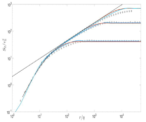
While the comparison between the present calculation and DNS data suggests good agreement, one can nevertheless notice that the DNS data for  $Re_\lambda =1100$, 1300 and 2250 lie slightly above the calculations for
  $r/\eta \geqslant 200$ before
  $S_2$ reaches its constant value at large
  $r/\eta$ where it must be
  $2u'^{2}$. This difference is more emphatically illustrated in figure 5 which shows the distributions of
  $S_2$ of figure 3 normalised by
  $(\bar {\epsilon } r)^{2/3}$. The decaying grid turbulence data of Kaminsky et al. (Reference Kaminsky, Birnir, Bewley and Sinhuber2020) at
  $Re_\lambda =1450$ are added. The value of
  $\bar {\epsilon }$ reported by Kaminsky et al. (Reference Kaminsky, Birnir, Bewley and Sinhuber2020) has been adjusted so that
  $S_2$ (before normalising by
  $(\bar {\epsilon } r)^{2/3}$) aligns with the other DNS data in the region
  $10 \leqslant r/\eta \leqslant 100$. The deviation of the present calculated distributions from the DNS data in the region
  $r/\eta \leqslant 10$ is expected, as explained earlier. The calculations show that, as
  $r/\eta$ increases,
  $S_2/(\bar {\epsilon } r)^{2/3}$ approaches a region over which it varies very slowly before decreasing again. The extent of this region increases with the Reynolds number. While the DNS data at
  $Re_\lambda = 335$ and the grid turbulence data behave similarly, the DNS data at
  $Re_\lambda = 1300$ and 2250 exhibit an ‘overshoot’ when compared to the calculated distributions. A similar behaviour is seen for the data of Ishihara et al. (Reference Ishihara, Kaneda, Morishita, Yokokawa and Uno2020) even when
  $Re_\lambda$ is as small as 675. Interestingly, the numerical simulations of HIT up to
  $Re_\lambda = 10^{6}$ based on an EDQNM (Meldi et al. Reference Meldi, Djenidi and Antonia2021) show the existence of a similar overshoot when HIT is forced (an example is shown in the figure); the overshoot is not observed for decaying HIT.

Figure 5. Distributions of  $S_2/(\bar {\epsilon } r)^{2/3}$. Solid lines and symbols are as in figure 2. Black crosses: grid turbulence data at
  $Re_\lambda =1450$ (Kaminsky et al. Reference Kaminsky, Birnir, Bewley and Sinhuber2020). Red dash-dotted line: EDQNM,
  $Re_\lambda =1131$.
The above comparison between the present calculations and the DNS data raises a paradox which, for convenience, is hereafter referred to as the  $S_2$ paradox. Indeed, even though the calculations and the DNS (and EDQNM) use the same forcing, there is no overshoot in the former. This is disconcerting since both the calculations and DNS have similar
  $S_3$ and
  $Z_r$ distributions in the region beyond the dissipative range, as seen in figures 1 and 4. This paradox and its resolution are considered in the next section.
3. The $S_2$ paradox

In the present calculations, the closed form of the KHEq is solved to obtain  $S_2$. However,
  $S_2$ can also be calculated, as done in EDQNM and DNS, from the three-dimensional energy spectrum,
  $E(k)$, as follows:
 \begin{equation} S_2 = 4 \int_0^{\infty} E(k) \left(\frac{1}{3} - \frac{\sin kr - kr \cos kr}{(kr)^{3}}\right)\textrm{d}k, \end{equation}
where  $k$ is the wavenumber. For the purpose of the analysis, a theoretical spectrum with and without forcing is considered. The unforced spectrum is that of Pope (Reference Pope2000):
 \begin{equation} E(k) = C\bar{\epsilon}^{2/3}k^{{-}5/3}f_L(kL)f_\eta(k\eta), \end{equation}
where  $C= 1.5$,
 \begin{equation} f_L(kL) = \left(\frac{kL}{[(kL)^{1.5}+c_L]^{1/1.5}}\right)^{2/3}k^{{5}/{3}+p} \end{equation}
and
 \begin{equation} f_\eta(k\eta) =\exp({-\beta([(k\eta)^{4}+c_\eta^{4}]^{1/4}-c_\eta)}), \end{equation}
with  $p=2$,
  $c_L=6.78$,
  $\beta =5.3$ and
  $c_\eta =0.4$. To emulate a forced spectrum we simply use
 \begin{equation} E_f(k)=\left(1+\frac{\gamma}{k}\right)E(k), \end{equation}
where  $\gamma$ can take any positive value to change the forcing intensity. This is simple but, as will be seen, sufficient to illustrate the effect of a low-wavenumber forcing on the calculation of
  $S_2$ via (3.1). Figure 6 shows the unforced and forced spectra for two largely different kinematic viscosity values that lead to a significant Reynolds number difference. The figure (inset) also reports the DNS data for forced HIT of Ishihara et al. (Reference Ishihara, Morishita, Yokokawa, Uno and Kaneda2016). We have used their data of
  $\bar {\epsilon }$ and
  $L$; for
  $Re_\lambda = 2297$ we used their value of
  $\nu = 4.1 \times 10^{-6}$; for
  $Re_\lambda = 7.264\times 10^{4}$ we simply reduced the viscosity to
  $\nu = 4.1 \times 10^{-9}$, while
  $\bar {\epsilon }$ and
  $L$ are unchanged. When forcing is applied, the forced spectra differ from the unforced spectra in the low-wavenumber region. This indicates that (3.5) emulates relatively well a spectrum of forced HIT (seen in the inset), and can represent the spectra obtained in the DNS and EDQNM simulations of forced HIT. Thus, both forced and unforced spectra can now be used to compute
  $S_2$ using (3.1) and the results are reported in figure 7 showing the distributions
  $S_2/(\bar {\epsilon } r)^{2/3}$ for different values of
  $\gamma$. We also show the EDQNM data for
  $Re_\lambda = 10^{4}$ of Meldi et al. (Reference Meldi, Djenidi and Antonia2021). In (3.2),
  $C$ is supposed to be equal to the Kolmogorov constant
  $C_K$. However, the value of 1.5 used in (3.2) is lower than the assumed value of
  $C_K \simeq 2$. Here, we also use
  $C=1.5$ since, in combination with the other (fitting) constants
  $p$,
$p$,  $c_L$,
  $\beta$ and
  $c_\eta$, it yields good agreement with DNS spectra as shown in figure 6. The actual value of
  $C$ is not important as it does not alter the shapes of the
  $S_2$ curves calculated with (3.1), which are the focus here, and as illustrated in figures 7(a) and 7(b) where we used
  $C=1.5$ and 1.63, respectively. The results of figure 7 illustrate the impact of forcing on
  $S_2$. Forcing increases the magnitude of
  $S_2/(\bar {\epsilon } r)^{2/3}$ when compared to the unforced spectra and can lead to a significant overshoot. Note though that the impact of forcing is practically negligible in the region
  $r/\eta \leqslant 10$. The effect of forcing becomes important for
  $r \geqslant 10 \eta$ and
  $r \geqslant 1000 \eta$ at lower and larger Reynolds numbers, respectively. The plots of figure 7 indicate that the larger the forcing intensity the deeper into the small scales its effect will be felt. It also indicates that the larger the Reynolds number the weaker this effect is on the small scales. Taking these considerations into account, one can argue that the DNS data shown in figure 5 present a trend towards
  $S_2/(\bar {\epsilon } r)^{2/3}$ and that higher-Reynolds-number DNS may confirm this trend.

Figure 6. Unforced ( $\gamma =0$) and forced (
 $\gamma =2$, 5 and 10) three-dimensional energy spectra for
  $Re_\lambda =2297$ (thick lines) and
  $7.264\times 10^{4}$ (thin lines). Inset: DNS data of Ishihara et al. (Reference Ishihara, Morishita, Yokokawa, Uno and Kaneda2016). Red circles,
  $Re_\lambda = 675$; blue triangles,
  $Re_\lambda = 2297$; black lines, unforced spectra for
  $Re_\lambda = 675$ and 2297.

Figure 7. Distributions of  $S_2/(\bar {\epsilon } r)^{2/3}$ computed with unforced and forced spectra. Lines are the same as in figure 6. Triangles, DNS data of Ishihara et al. (Reference Ishihara, Kaneda, Morishita, Yokokawa and Uno2020),
  $Re_\lambda =2297$; pink dash-dotted line, EDQNM data of Meldi et al. (Reference Meldi, Djenidi and Antonia2021),
  $Re_\lambda = 10^{4}$. The arrow indicates the direction of increasing
  $\gamma$. (a) Parameter
  $C$ in (3.2) is equal to 1.5; (b)
  $C= 1.63$ and only the cases for
  $\gamma =0$ and 10 are shown with the DNS and EDQNM data.
The message of figure 7 is clear: the external spectral forcing applied at lower wavenumbers can lead to an overshoot in the  $S_2/(\bar {\epsilon } r)^{2/3}$ distributions when compared to the no forcing case. This nevertheless does not yet explain the
  $S_2$ paradox. But it should be recalled that the KHEq has been developed in the context of a decaying turbulence which is isotropic at all scales of motion. In this context, not only should the large-scale motion be isotropic, but its energy should decay in time. Thus, its contribution, i.e. the third term on the left-hand side of (1.1), also decays in time. Replacing this term by another one to emulate a steady-state isotropic turbulence thus changes the nature of the equation. For example, the integral term, which is a cumulative term, depends on
  $S_2$, while the replacing term (2.6) is neither cumulative nor
  $S_2$-dependent. This reminds us that the extra term commonly added to the Navier–Stokes equations (from which, we should recall, (1.1) is derived) to emulate external forcing at large scales is unnatural (Lamorgese, Caughey & Pope Reference Lamorgese, Caughey and Pope2005). It is worth remembering that its use is justified on the basis that it has little effect on the small-scale statistics. Clearly, the results of figure 7 contradict this view, particularly when the Reynolds number is not large enough. The change in the nature of the KHEq when the forcing term is added can be illustrated by considering the following equation in the region beyond the dissipative range, where the viscous term in (1.1) can be dropped:
 \begin{equation} S_3 - Z_r ={-} \tfrac{4}{5} \bar{\epsilon} r. \end{equation}
For decaying isotropic turbulence,  $Z_r$ is given by the integral term in (1.1) and (3.6) is the transport equation of
  $S_2$ with
  $S_3$ unknown. On the other hand, if
  $Z_r$ is given by (2.6), then (3.6) is not a transport equation for
  $S_2$ since
  $S_2$ does not appear in the equation. In fact, (3.6) can be used to obtain
  $S_3$, as done in § 2, irrespective of
  $S_2$ which, as far as this equation is concerned, is undetermined and thus can have any value. This remark concerning the change in the nature of the KHEq echoes Reference PopePope's (Reference Pope2000) reminder that the large-scale energy-containing motions generated in the spectral domain by low-wavenumber forcing are unnatural and not governed by the Navier–Stokes equations. In that context, it is not surprising that the KHEq solutions do not agree with numerical simulations where a turbulence field is generated by an external forcing such as in DNS and EDQNM calculations. Only if the Reynolds number is large enough can the KHEq, DNS and EDQNM solutions be in agreement in the dissipative and scaling ranges, as indeed figures 5 and 7 would suggest.
We complete this section by solving the KHEq where  $Z_r$ is given by the linear isotropic forcing used by Lundgren (Reference Lundgren2003):
 \begin{equation} Z_r=\frac{2\bar{\epsilon}}{u'^{2}}\frac{1}{r^{4}}\int_0^{r} s^{4}S_2\,\textrm{d}s. \end{equation}
Lundgren suggests that this forcing is equivalent to a uniform spectral forcing at all wavenumbers and can allow comparison with decaying HIT. Notice the cumulative aspect of this expression, mimicking the integral term in (1.1). Figure 8 shows  $Z_r$ for both linear and spectral forcing. Both types of forcing lead to the correct limit,
  $Z_r = (4/5)(\bar {\epsilon }r)$, as they should, at large
  $r/\eta$ but they result in significantly different behaviours as
  $r/\eta$ decreases. They decrease at different rates with decreasing
  $r/\eta$. For example, as
  $r/\eta$ decreases,
  $Z_r$ remains larger for the spectral than for the linear forcing until
  $r/\eta \simeq 0.6 \times 10^{4}$. Below this value,
  $Z_r$ is smaller with the linear forcing. One can expect that this behaviour should be reflected in the distributions of
  $S_2$. This is indeed observed in figure 9 which shows distributions of
  $S_2$ normalised by
  $v_K$. As the large scales are approached, the calculations based on the spectral forcing yield systematically higher values of
  $S_2$ than when the linear forcing is used. This was also observed by Lundgren (Reference Lundgren2003), although the observation was made with regard to the approach to the four-fifths law. Notice that in an attempt to improve the calculation in the dissipative range, we used the boundary condition
  $S_2=({1}/{15\nu })\bar {\epsilon }r^{2}$ at
  $r = \eta$, which is the correct solution of the KHEq in the dissipative range where the first and third terms on the left-hand side of (1.1) are negligibly small. A comparison with figure 3 indicates that this simple change of boundary condition improves the calculation in the dissipative range. Also reported in figure 9 are the experimental data of grid turbulence (Djenidi, Kamruzzaman & Antonia Reference Djenidi, Kamruzzaman and Antonia2015; Kaminsky et al. Reference Kaminsky, Birnir, Bewley and Sinhuber2020) and round jet centreline (Djenidi et al. Reference Djenidi, Antonia, Lefeuvre and Lemay2016). Adding a forcing term to the Navier–Stokes equations is equivalent to introducing energy. This energy is then distributed among all scales of motion. But, as illustrated by
  $Z_r$, this distribution is not uniform among the scales of motion; the larger the scales the more energy they receive. This is well reflected in the distributions of
  $S_2/v_K^{2}$. The calculated (forced) distributions exhibit higher values of
  $S_2/v_K^{2}$ than the measured (decaying) distributions in the range of scales delimited by the dissipative range and the very large scales where
  $S_2$ becomes constant. Interestingly, the agreement between calculation and measurement is better for the jet flow than grid turbulence, suggesting that the large-scale contribution is stronger in the former flow.


Figure 9. Distributions of  $S_2$ computed via (1.1) with spectral forcing (red lines) and linear forcing (blue lines). Symbols are experimental data of grid turbulence and round jet.
4. Concluding discussion
A closed form of the KHEq is solved to investigate the behaviour of the second-order velocity structure function,  $S_2$, in HIT at finite Reynolds numbers. The closure model is based on a gradient type with an eddy viscosity formulation proposed by Djenidi & Antonia (Reference Djenidi and Antonia2021). The results are in good agreement with experimental data (figure 9). Further, they indicate that when the Reynolds number is large,
  $S_2$ behaves like
  $(\bar {\epsilon }r)^{2/3}$ in a range of scales beyond the dissipative range and well before the scale range where
  $S_2$ becomes constant, thus supporting the existence of a two-thirds law when the Reynolds number is very, if not infinitely, large. However, comparison with the DNS data for forced HIT reveals a paradox: while both the KHEq and DNS use the same isotropic spectral forcing, the DNS data exhibit larger values of
  $S_2$ than the KHEq solutions in the region where
  $S_3/(\bar {\epsilon }r)$ starts to decrease with increasing
  $r$ (figure 1), which is illustrated by an overshoot in
  $S_2/(\bar {\epsilon }r)^{2/3}$ (figure 5). Calculations of
  $S_2$ via the energy spectrum (3.1) reveal similar overshoots in
  $S_2/(\bar {\epsilon }r)^{2/3}$ when forced spectra are used (figure 7); also, the stronger the forcing intensity the larger the magnitude of the overshoot. These results strongly suggest that the overshoot exhibited by the DNS data is associated with the forced energy spectrum. As the Reynolds number increases, and for a given spectral forcing applied at the same low wavenumbers, the overshoot shifts to larger values of
  $r/\eta$ allowing
  $S_2$ to approach its infinite-Reynolds-number behaviour, i.e.
  $(\bar {\epsilon }r)^{2/3}$, in the scaling range. This discussion about the overshoot in the distributions of
  $S_2/(\bar {\epsilon }r)^{2/3}$ raises a pertinent question: why do the DNS data for
  $S_3/(\bar {\epsilon }r)$ not show an overshoot when forcing is applied? Moment
  $S_3$ is associated with the transfer of energy, not with the energy itself, so that the actual mechanism of energy transfer among scales is the same regardless of whether the energy spectrum is forced or not; there is simply more energy to transfer when forcing is used.
An interesting point that stems from the present study concerns the two-thirds law. The KHEq solutions clearly show that as long as turbulence is isotropic at all scales of motion, this law can be well approximated at large Reynolds numbers; it is better approximated in forced than in decaying turbulence, as seen in figure 9. Also, the presence of the large-scale anisotropy disrupts this. Indeed, the effect of this anisotropy can penetrate deep into the small scales, particularly if the Reynolds number is not large. This unfortunately complicates the interpretation of comparisons between the (isotropic) Kármán–Howarth predictions and the actual results in anisotropic flows.
Finally, the present results, and in particular the calculations of  $S_2$ based on the forced three-dimensional energy spectrum, suggest that the current DNS data are not inconsistent with a trend towards the two-thirds law. It is possible that the current DNS Reynolds numbers are not large enough to avoid the effect of forcing on the small scales beyond the dissipative range and thus disrupting the behaviour of
  $S_2$ in the so-called scaling range; this effect increases as the size of the scale increases. DNS data at much larger Reynolds numbers than the current ones will certainly help clarify the issue of how forcing affects the scaling range.
Declaration of interests
The authors report no conflict of interest.


