


1. Introduction
Geological strata represent a valuable resource, not only in terms of the mineral wealth that they may contain, but also in terms of their ability to (seasonally) store internal energy (MacKay Reference MacKay2009) and to (permanently) store anthropogenic pollutants. In this latter capacity, much attention has been paid to the sequestration of supercritical carbon dioxide ( $\textrm {CO}_2$) in various locales, e.g. China, Canada, Norway, Australia, the United States and the United Kingdom (Tang, Yang & Bian Reference Tang, Yang and Bian2014). Less thoroughly studied in the academic literature, though still important, is the disposal of acid gas in depleted oil and gas reservoirs or deep saline aquifers. Acid gas injection often occurs in land-locked regions located on sedimentary basins, such as Labarge, Wyoming, USA (Parker et al. Reference Parker, Northrop, Valencia, Foglesong and Duncan2011) and in the Alberta Basin in Western Canada (Bachu et al. Reference Bachu, Buschkuehle, Haug and Michael2008b). In either case, acid gas injection operations are often thought to represent a small-scale analogue of
  $\textrm {CO}_2$ sequestration. To this end, and for both acid gas and
  $\textrm {CO}_2$ sequestration, concerns persist related to the long-term confinement of fluid injected deep underground. Such concerns are exacerbated by the difficulty and expense of monitoring injectate migration and the uncertainties inherent with forward-simulating numerical models (Bachu et al. Reference Bachu, Buschkuehle, Haug and Michael2008a). Thus, there is an ongoing need for comparatively simple analytical models that provide qualitative and quantitative insights into the nature of buoyancy-driven flow in porous media.
When a light or dense fluid is injected into a porous medium, its subsequent migration depends on various factors, such as pressure and temperature, solubility, the interplay between hydrodynamic and buoyancy forces and the heterogeneity of the medium. When, as is typical, density differences arise, the injectate may migrate in the form of a vertical plume or in the form of horizontal or sloping gravity current(s). Indeed, one may feed the other as when a plume strikes an impermeable boundary (Sahu & Flynn Reference Sahu and Flynn2015) or permeability jump (Sahu & Flynn Reference Sahu and Flynn2017) or when a gravity current drains from the edge of an impermeable lens (Hesse & Woods (Reference Hesse and Woods2010), and see also figures 10.10 and 10.11 of Woods (Reference Woods2014)).
Gravity currents in porous media have been studied widely in the past decades both experimentally and theoretically. One of the earliest investigations was conducted by Huppert & Woods (Reference Huppert and Woods1995), who examined the short- and long-term spreading behaviour of gravity currents along both horizontal and inclined impermeable boundaries. Since the publication of this pioneering work, numerous follow-up studies have been conducted to explore the effect of, for example, a time-varying source (Vella & Huppert Reference Vella and Huppert2006), density stratification within the gravity current (Pegler, Huppert & Neufeld Reference Pegler, Huppert and Neufeld2016) and vertical confinement (Nordbotten & Celia Reference Nordbotten and Celia2006; Zheng et al. Reference Zheng, Guo, Christov, Celia and Stone2015). Also, and although it is theoretically and experimentally expedient to assume the boundaries confining the gravity current to be impermeable, there are numerous practical situations wherein leakage may occur through large faults or high-permeability zones in cap rock (Fitts & Peters Reference Fitts and Peters2013; Espinoza & Santamarina Reference Espinoza and Santamarina2017); in such cases drainage must be considered. To this end, studies have focused on the case of an isolated (Vella et al. Reference Vella, Neufeld, Huppert and Lister2011) versus a distributed sink. In the latter case, Pritchard, Woods & Hogg (Reference Pritchard, Woods and Hogg2001), Neufeld & Huppert (Reference Neufeld and Huppert2009) and Farcas & Woods (Reference Farcas and Woods2009) studied the flow of a gravity current over a thin permeable layer. The extension to the thick lower layer case has been explored by Goda & Sato (Reference Goda and Sato2011) and Sahu & Flynn (Reference Sahu and Flynn2017) among others. Whatever the lower layer thickness, the draining flow from the underside of the gravity current has been modelled by considering the flow to be driven by the hydrostatic head of the overlying gravity current (Acton, Huppert & Worster Reference Acton, Huppert and Worster2001; Pritchard et al. Reference Pritchard, Woods and Hogg2001; Goda & Sato Reference Goda and Sato2011). In case of a thick lower layer, the source fluid is pulled both along and across the interface between the two layers, which we call the permeability jump, and the gravity current ultimately reaches a terminal or run-out length. As suggested by the name, the run-out length is the horizontal distance at which the volume of fluid supplied to the gravity current is just balanced by that draining from underneath. Whereas the case of a horizontal permeability jump has been studied by Goda & Sato (Reference Goda and Sato2011) and Sahu & Flynn (Reference Sahu and Flynn2017), there are numerous geological examples where the permeability jump makes a non-trivial angle to the horizontal. These examples include the Wabamun groups (Bachu et al. Reference Bachu, Buschkuehle, Haug and Michael2008a) in Western Canada, which are used as repositories for acid gas, the Entrada and Weber formations in the United States Rocky Mountain region (McPherson & Matthews Reference McPherson and Matthews2013) and China's Shiqianfeng group in the Ordos Basin (Jing et al. Reference Jing, Yang, Tang and Wang2019) all of which are used as repositories for supercritical  $\textrm {CO}_2$. For the examples just cited, the regional dip angles vary from as little as
  $0.4^\circ$ to as much as
  $20^\circ$.
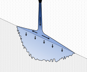
In light of the above examples, it is surprising that more attention has not been paid to the (asymmetric) problem of gravity current propagation along a sloping, permeable boundary. Adding to the flow complexity is the possibility that the up- and downdip gravity currents are fed by a plume rather than by an isolated source located along the permeability jump itself. A schematic of this flow is illustrated in figure 1. Here, and consistent with the laboratory experiments to be described later, we consider a source of dense fluid located significantly above the permeability jump that leads to the formation of a descending plume in the upper layer. On the other hand, such details of orientation are irrelevant provided that density differences are modest so that the flow is Boussinesq. Note also from figure 1 that the plume and gravity currents feed back upon each other and the composite problem is therefore more nuanced than either constituent part.

Figure 1. Schematic of discharged plume fluid propagating as a pair of leaky gravity currents along an inclined permeability jump. The colourbar on the right-hand side indicates the variation in density as the source fluid migrates within the porous medium.
Addressing the above described open problem is the primary objective of the present study. Precise goals include (i) characterizing the relative up- versus downdip flow as a function of  $\theta$, the permeability jump angle, and (ii) resolving the time-dependent advance of the up- and downdip gravity currents until the respective run-out lengths are reached. As part of the analysis, key differences with the horizontal permeability jump case will be highlighted. Complementing the above analysis, our study also includes similitude laboratory experiments. Although their ostensible purpose is to provide data to corroborate the theoretical model, we shall see that the experimental images reveal behaviour that highlights the limitations of considering a sharp interface in the gravity current model.
The rest of the paper is organized as follows. In § 2, we derive a theoretical model for the flow in question and discuss some of the key model predictions in § 3. Section 4 describes the laboratory experiments and the techniques used to analyse experimental images along with a qualitative comparison with the theory. Quantitative comparisons are reserved for § 5. Section 6 presents an overarching summary in which ideas for future study are briefly outlined.
2. Theoretical modelling
2.1. Problem description
To theoretically model the flow described in figure 1, we consider a two-layer porous medium with notation as illustrated schematically in figure 2. The permeability and porosity in the upper layer are  $k_1$ and
  $\phi _1$, respectively, while the corresponding values in the lower layer are
  $k_2$ and
  $\phi _2$, respectively. The permeability jump makes a constant angle
  $\theta$ with the horizontal. The natural coordinate system in two-dimensional space is represented by (
 ${X,Z}$), where the vertical Z-axis is aligned anti-parallel to the gravitational acceleration
  $g$. For reference, note that the coordinate system (
 ${x,z}$) associated with the along- and cross-jump directions is obtained from (
 ${X,Z}$) by a clockwise rotation of
  $\theta$ about the Y -axis,
  $Y$ being the direction normal to the page. Coordinate rotation can be expressed mathematically using a transformation matrix, i.e.
 \begin{equation} \begin{bmatrix}{x} \\ {z}\end{bmatrix} = \begin{bmatrix} \mathrm{cos}\ \theta\ & \sin \theta \\ -\sin \theta\ & \cos \theta \end{bmatrix} \begin{bmatrix} {X} \\ {Z} \end{bmatrix}. \end{equation}
We position the origin of both coordinate systems on the permeability jump, directly below the dense line source, which is itself is positioned at ( $X=0, Z=H$), see figure 2.

Figure 2. Definition schematic showing the propagation of discharged plume fluid in the up- and downdip directions along the inclined permeability jump. Draining into the lower layer is also indicated.
Our theoretical model is predicated on the following simplifying assumptions. (i) Although the upper and lower layers are assumed to support different permeabilities, the porosities are assumed equal, i.e.  $\phi _1 = \phi _2 \equiv \phi$. (ii) The upper and lower layers are assumed to be very deep in vertical extent (Goda & Sato Reference Goda and Sato2011); the consequences of assuming otherwise will be briefly highlighted in § 4. (iii) Initially, the entire porous medium is assumed to be uniformly saturated with ambient fluid of density
  $\rho _{o}$. (iv) The source and ambient fluids have equal dynamic viscosities and are assumed to be fully miscible so that effects due to capillarity can be ignored. (v) When the plume strikes the permeability jump at
  $x=0$, all of its fluid is then discharged in the form of flows propagating up- and down-dip; this assumption is defensible provided
  $k_2/k_1 \ll 1$, see for example figure 3 of Sahu & Flynn (Reference Sahu and Flynn2017). (vi) The so produced up- and downdip gravity currents remain long and thin. (vii) Consistent with Bear (Reference Bear1972), Woods & Mason (Reference Woods and Mason2000), Pritchard et al. (Reference Pritchard, Woods and Hogg2001) and De Loubens & Ramakrishnan (Reference De Loubens and Ramakrishnan2011), gravity current fluid is at all times separated from overlying ambient fluid by a sharp interface. (viii) The density difference between the source fluid and the ambient fluid is moderate and the flow remains Boussinesq everywhere in the domain. (ix) Spatial variations in the density within the up- and downdip gravity currents and within the contaminated fluid consisting of discharged plume fluid that has drained into lower layer are modest and can be ignored to leading order.
The plume line source discharges fluid of density  $\rho _s>\rho _o$ at a constant volume flux per unit width,
  $q_{s}$. The source buoyancy flux per unit source width is
  $F_s=q_{s} {g}^\prime _{s}$, where
  $g'_s= g (\rho _s-\rho _o)/\rho _o\ll {g}$ is the source reduced gravity. As the dense fluid falls downwards, entrainment occurs as a result of which the volume flux of the resulting plume increases with the vertical distance from the source. Using a boundary layer approximation, Wooding (Reference Wooding1963) derived an expression to predict this variation in the limit of small Péclet number, i.e.
  ${Pe}=U d_o\tau /D_m \ll O(1)$, where
  $U$ is a characteristic velocity,
  $d_o$ is the mean grain diameter,
  $D_m$ is the molecular diffusivity. Further,
  $\tau > 1$ is the (hydraulic) tortuosity, which is defined as the square of the hydraulic flow path length to the corresponding straight line length (Carman Reference Carman1937) or as the product of porosity and a formation factor (Clennell Reference Clennell1997; Ghanbarian et al. Reference Ghanbarian, Hunt, Ewing and Sahimi2013). Later, Sahu & Flynn (Reference Sahu and Flynn2015) derived a similar relation for
  ${Pe}\gg O(1)$ and also proposed a relation for the variation of the plume reduced gravity with
  $Z$. Herein, we model the flow assuming
  ${Pe}\gg O(1)$, see § 2.4.
When the plume strikes the permeability jump, discharged plume fluid is divided into equal ( $\theta ={0}^{\circ }$) or unequal (
 $\theta \neq {0}^{\circ }$) flows to the right and left. The discharged plume fluid propagates as a pair of leaky gravity currents under a balance of buoyancy and viscosity with simultaneous draining into the lower layer. The pressure is continuous along
  $z=h(x,t)$ where
  $h$ denotes the gravity current height, measured perpendicular to the permeability jump, see figure 2. Because of the continual addition of fluid from above,
  $h$ steadily increases with time,
  $t$. Consequently, and because the density,
  $\rho _p$, and plume volume flux per unit width,
  $q_p$, vary with the vertical coordinate due to entrainment, the fluid feeding the gravity current has a density that slowly increases with time and a volume flux that slowly decreases with time. The influx density is denoted by
  $\rho _p(h_{0})$ with a corresponding volume flux per unit width denoted by
  $q_p(h_{0})$ where
  $h_0 \equiv h(x=0,t) \equiv h_0(t)$ is the time-dependent gravity current height measured directly below the plume source. The volume influx
  $q_p(h_0)$ is obviously the same
  $q_c$. In a similar spirit, and neglecting spatial variations of the gravity current density, we have that
  $\overline {\rho _c} = \rho _p(h_{0})$ where
  $\rho _o < \overline {\rho _c} <\rho _s$. Although the spatially uniform approximation is clearly a theoretical simplification relative to the real flow, we expect internal stratification effects to be relatively minor provided
  $H$ is not small. With this assumption to hand, the average density difference between the up- and downdip gravity currents and the ambient fluid is
  ${\rm \Delta} \overline {\rho _c} = \overline {\rho _{c}}-\rho _{o}$ and the corresponding reduced gravity is
  $\overline {g'_c}=g ({\rm \Delta} \overline {\rho _c}/\rho _o)$.
Below the permeability jump, there is a draining of discharged plume fluid into the lower layer. The draining flow displaces less dense ambient fluid thereby creating an unstable interface leading to Rayleigh–Taylor type fingering (Saffman & Taylor Reference Saffman and Taylor1958; Homsy Reference Homsy1987), see figure 1. Occurrence of similar fingering phenomena has been observed previously for gravity currents propagating along a horizontal permeability jump (Sahu & Flynn Reference Sahu and Flynn2017) or along the underside of a sloping, impermeable boundary (MacMinn & Juanes Reference MacMinn and Juanes2013). A consequence of the fingers is that some mixing of draining discharged plume fluid and ambient fluid must occur. To distinguish the less dense discharged plume fluid in the lower layer from that more dense discharged plume fluid in the upper layer, we shall, in the lower layer, make reference to contaminated fluid, which in figure 2 is characterized by a depth  $l$. By contrast, when we refer to discharged plume fluid, it should hereafter be understood that we refer specifically to the upper layer.
As a further consequence of the mixing described above, we cannot, strictly speaking, assume a sharp interface in the lower layer, cf. figure 1. Nonetheless, and for theoretical expediency, we assume a spatially uniform mixing process in the lower layer and thereby define an average interface location for the contaminated fluid relative to the ambient, see figure 2. The average density of the contaminated fluid is  $\overline {\rho _d}<\overline {\rho _c}$ and the corresponding density difference with the ambient fluid is
  ${\rm \Delta} \overline {\rho _d} = \overline {\rho _d }- \rho _o$. Thus the mean reduced gravity of the draining fluid is expressed as
  $\overline {g'_d}=g ({\rm \Delta} \overline {\rho _d}/\rho _o)<\overline {g'_c}$. Determination of
  $\overline {\rho _d}$ and
  $\overline {g'_d}$ will be discussed below.
2.2. Gravity currents
Consider, as in figure 2, a two-dimensional flow of the gravity currents propagating along the permeability jump in the upper layer along the up- and downdip directions. Let the Darcy velocity of the gravity currents be  ${{\boldsymbol {u}}}_c\equiv ({u}_{c},{w}_{c})$, with components
  $u_c$ and
  $w_c$ in the along- and cross-jump directions, respectively. As noted above, the gravity currents are assumed long and thin (small aspect ratio,
  $\varepsilon = \text {height/length} \ll 1$). As a consequence, and consistent with the Dupuit approximation (see Bear (Reference Bear1972) and appendix A.3)
  ${w}_{c}$ can be considered small compared with
  ${u}_{c}$ and the cross-layer pressure gradient within each gravity current can be considered approximately hydrostatic (Huppert & Woods Reference Huppert and Woods1995). Considering the along-jump flows in a rotated coordinate system for
  $\theta > {0}^{\circ }$, we define the hydrostatic pressure in the cross-flow direction as
 \begin{equation} {P}_c(x,z,t)={p}_{c}(x,t)-\overline{\rho_c} g z\cos \theta. \end{equation}
Here,  $p_c(x,t)$ is given by
 \begin{equation} {p}_{c}(x,t)= P_o+ (\overline{\rho_c}-{\rm \Delta}\overline{\rho_c}) {g}x\sin \theta+ {\rm \Delta} \overline{\rho_c} g h \cos \theta, \end{equation}
where  $P_o$ is the pressure measured at the origin. Using Darcy's law, it can be shown that the along-jump flow velocities with the up- and downdip gravity currents are
 \begin{equation} u_c= -\frac{k_{1}
{\rm \Delta} \overline{\rho_c} g}{\mu} \begin{cases}
\displaystyle \frac{\partial{h}}{\partial{x}}\cos \theta +
\sin \theta, & [\text{updip}, -x_{N_u} < x < 0] \\ \displaystyle
\frac{\partial{h}}{\partial{x}}\cos \theta - \sin \theta, &
[\text{downdip}, 0 < x < x_{N_d}] \end{cases}
\end{equation}
\begin{equation} u_c= -\frac{k_{1}
{\rm \Delta} \overline{\rho_c} g}{\mu} \begin{cases}
\displaystyle \frac{\partial{h}}{\partial{x}}\cos \theta +
\sin \theta, & [\text{updip}, -x_{N_u} < x < 0] \\ \displaystyle
\frac{\partial{h}}{\partial{x}}\cos \theta - \sin \theta, &
[\text{downdip}, 0 < x < x_{N_d}] \end{cases}
\end{equation}
where  $\mu$ is dynamic viscosity and
  $x_{N_u}$ and
  $x_{N_d}$ are the nose locations in the up- and downdip directions, respectively, see figure 2. The velocities prescribed by (2.4) apply for
  $z < h$. Because the upper layer is assumed semi-infinite, the velocity within the ambient is considered negligible (cf. De Loubens & Ramakrishnan Reference De Loubens and Ramakrishnan2011). To derive an evolution equation for
  $h$, we take the depth average of the mass conservation equation, similar to (2.6) of Huppert & Woods (Reference Huppert and Woods1995), and consider mass loss due to draining from the gravity current undersides. Upon substituting (2.4) into the resulting depth-averaged equation, we obtain
 \begin{equation} \phi \frac{\partial{h}}{\partial{t}}= \begin{cases} \displaystyle \frac{k_{1} \overline{g'_c}}{\nu} \frac{\partial{}}{\partial{x}} \left(h\frac{\partial{h}}{\partial{x}}\cos \theta +h \sin \theta \right) + w_{drain}, & [\text{updip}, -x_{N_u} < x < 0] \\ \displaystyle \frac{k_{1} \overline{g'_c}}{\nu} \frac{\partial{}}{\partial{x}}\left( h\frac{\partial{h}}{\partial{x}}\cos \theta -h \sin \theta \right) + w_{drain}, & [\text{downdip}, 0 < x < x_{N_d}] \end{cases} \end{equation}
where  $\nu =\mu /\rho _o$ denotes the kinematic viscosity and
  $w_{drain}$ is the draining velocity, an expression for which is provided in the following subsection.
2.3. Draining flow in the lower layer
Here, we evaluate the time evolution of the average position of the interface between the contaminated and the ambient fluids in the lower layer. The Darcy velocity of the contaminated fluid in the lower layer is  ${{\boldsymbol {u}}}_d\equiv ({u}_{d},{w}_{d})$, having components
  $u_d$ and
  $w_d$ in the along- and cross-jump directions, respectively. For
  $\theta ={0}^{\circ }$, the along-jump velocity in the lower layer
  $u_{d}$ is considered by Acton et al. (Reference Acton, Huppert and Worster2001) to depend only on the horizontal gradient of the hydrostatic pressure exerted by the gravity current, i.e.
  $\partial {h}/\partial {x}$. Meanwhile, the cross-jump component of velocity,
  $w_{d}$, depends not on
  $\partial h/\partial x$ but rather on
  $h$. Because
  $\partial {h}/\partial {x}$ can be shown to be both approximately constant and small compared with unity,
  $|{u}_{d}|\ll \lvert {w}_{d} \rvert$. Consequently, the influence of
  ${u}_{d}$ on the draining velocity has typically been ignored in previous works. However, for inclined permeability jumps (
 $\theta \neq {0}^{\circ }$), the along-jump velocities may be significant because they include gravitational acceleration projected into the along-jump direction. Using Darcy's law, the along-jump velocities just below the jump boundary are given by
 \begin{equation} u_d= -\frac{k_{2} {\rm \Delta}\overline{\rho_d }g}{\mu} \begin{cases} \displaystyle \frac{\partial{h}}{\partial{x}}\cos \theta + \sin \theta, & [\text{updip}, -x_{N_u} < x < 0] \\ \displaystyle \frac{\partial{h}}{\partial{x}}\cos \theta - \sin \theta, & [\text{downdip}, 0 < x < x_{N_d}]. \end{cases} \end{equation}
Meanwhile, the cross-jump component is given by
 \begin{equation} {w}_{d}=-\frac{k_{2} {\rm \Delta}\overline{\rho_d }g}{\mu} \left( 1 + \frac{h}{l'} \right)\cos \theta, \end{equation}
where  $l'$ is the depth of the contaminated fluid as measured below and perpendicular to the permeability jump, see figure 2. In contrast to the case of a horizontal permeability jump,
  $|{u}_{d}| \approx \lvert {w}_{d} \rvert \tan \theta$, so that
  $|{u}_{d}|$ can be neglected only for relatively modest
  $\theta$. For larger
  $\theta$,
  ${u}_{d}$ becomes significant and needs to be considered when modelling the draining flow. In such cases, the net draining flow velocity
  $w_{drain}$ is influenced by both the along-jump velocity and the hydrostatic head in the cross-jump direction. To evaluate
  $w_{drain}$, we take the resultant of these two velocities, i.e.
  $\sqrt {{u}^2_{d}+{w}^2_{d}}$. Consistent with figure 2, it can be shown that for draining lengths significantly greater than the gravity current height, the direction of
  $w_{drain}$ remains vertical and its length is given as
  $l=l'/\cos \theta$. Taking these factors into consideration, the draining velocity can be written as
 \begin{equation} w_{drain}=-\frac{k_{2} {\rm \Delta}\overline{\rho_d}g}{\mu} \left(1 + \frac{h}{l} \cos \theta \right). \end{equation}
In the limiting case when  $\theta =0^{\circ }$, (2.8) reverts back to the expression used in previous works (Goda & Sato Reference Goda and Sato2011; Sahu & Flynn Reference Sahu and Flynn2017).
At the contaminated–ambient fluid interface, the volume flow rate per unit width,  $q_{entr}$, of the ambient fluid that mixes into the draining gravity current fluid can be expressed in terms of
  $w_{drain}$ as
 \begin{equation} q_{entr}=\frac{{\rm \Delta}\overline{\rho_c} - {\rm \Delta}\overline{\rho_d}}{{\rm \Delta} \overline{\rho_d}}\int_{-x_{N_u}}^{x_{N_d}} w_{drain} \,\mathrm{d}x, \end{equation}
see appendix A.1. The entrainment prescribed by  $q_{entr}$ is important because it, along with
  $w_{drain}$, dictates the time rate of increase of the draining fluid length,
  $l$. Following the derivation of appendix A.1 and incorporating (2.8), it can ultimately be shown that
  $l$ satisfies the following evolution equation:
 \begin{equation} \displaystyle \phi \frac{\partial{l}}{\partial{t}} = - \frac{\overline{g'_c}}{\overline{g'_d}}w_{drain}= \frac{k_{1} \overline{g'_c}}{\nu}\frac{k_{2} }{k_{1}}\left( 1 + \frac{h}{l} \cos \theta \right). \end{equation}
As with (2.5), (2.10) is valid in the range  $-x_{N_u}<x<x_{N_d}$.
2.4. Gravity currents and draining flows fed by a descending plume
Recall that the density of the fluid supplied to the gravity currents slowly increases with time as a result of the gradual increase of  $h$. Wishing to account for this fact in the governing equations (2.5) and (2.10) we adopt (2.25) of Sahu & Flynn (Reference Sahu and Flynn2015), and write
 \begin{equation} \displaystyle {g}^\prime_{c}=\left[\left(\frac{{\rm \pi} F_{s} \nu}{16 k_{1}} \right) ^2 \frac{1}{ \phi \alpha (H+ {Z}_{s} - h_0\cos \theta)}\right]^{{1}/{4}}. \end{equation}
Here, the source correction term  ${Z}_{s}= ({1}/{\phi \alpha}) ({{\rm \pi} \nu }/{16 F_{s} k_{1}})^2 q_{s}^{4}$ is evaluated considering the volumetric flow rate
  $q_s$ at the plume source. Also,
  $\alpha$ is the transverse dispersivity, whose connection to the porous medium grain size is discussed below in § 5.1. Substituting (2.11) into (2.5) and (2.10) yields, after some simplification,
 \begin{equation} \frac{\partial{h}}{\partial{t}}= \displaystyle \begin{cases} \displaystyle \beta (1- \chi h_{0^-}\cos \theta) ^{-{1}/{4}} \left[\frac{\partial{}}{\partial{x}}\left( h\frac{\partial{h}}{\partial{x}}\cos \theta +h \sin \theta \right) - K G^{\prime} \left(1 + \frac{h}{l}\cos \theta \right) \right],\\ \quad [\text{updip}, -x_{N_u} < x < 0], \\ \displaystyle \beta (1- \chi h_{0^+} \cos \theta) ^{-{1}/{4}} \left[\frac{\partial{}}{\partial{x}}\left(h\frac{\partial{h}}{\partial{x}}\cos \theta -h \sin \theta \right) - K G^{\prime} \left(1 + \frac{h}{l} \cos \theta \right) \right], \\ \quad [\text{downdip}, 0 < x < x_{N_d}], \end{cases} \end{equation}
and
 \begin{equation} \frac{\partial{l}}{\partial{t}}= \displaystyle \beta K \begin{cases} \displaystyle (1- \chi h_{0^-} \cos \theta)^{-{1}/{4}} \left(1 + \frac{h}{l} \cos \theta \right) , & [\text{updip}, -x_{N_u}< x < 0], \\ \displaystyle (1- \chi h_{0^+} \cos \theta) ^{-{1}/{4}} \left(1 + \frac{h}{l} \cos \theta \right) , & [\text{downdip}, 0 < x < x_{N_d}]. \end{cases} \end{equation}
Here  $\beta$ is a velocity parameter,
  $\chi$ is a source parameter,
  $K$ is the ratio of the lower to upper layer permeabilities and
  $G^{\prime }$ is the ratio of the lower to upper layer reduced gravities. More precisely, and in symbols,
 \begin{align} \displaystyle \beta= \frac{k_{1} }{\phi \nu} \left[\left(\frac{{\rm \pi} F_{s} \nu}{16 k_{1}} \right) ^2 \frac{ 1}{ \phi \alpha (H+Z_{s})}\right]^{{1}/{4}} ,\quad \displaystyle \chi =\frac {1}{H+Z_{s}},\quad \displaystyle K=\frac{k_{2}}{k_{1}},\quad \displaystyle G^{\prime} = \frac{\overline{g'_d}}{\overline{g'_c}}. \end{align}
Regarding the permeability jump angle  $\theta$ as a further independent parameter, there are a total of five variables in the governing equations (2.12) and (2.13).
2.5. Initial and boundary conditions
Recalling the initial condition of the porous medium to be uniformly saturated by ambient fluid, we initialize the gravity current height and draining length to zero, i.e.  $h=l=0$ at
  $t=0$. For
  $t>0$, (2.12) and (2.13) are solved using an influx boundary condition, which requires the time rate of volume increase of the up- and downdip gravity currents to balance the volume of fluid supplied by the descending plume. The plume volume flux per unit width,
  $q_c$, supplied at
  $x=0$, increases with distance from the source. Analogous to (2.11),
  $q_c$ can be expressed in terms of
  $h_0$ using
 \begin{equation} {q}_{c}= \left[\left(\frac{16 F_{s}k_{1}}{{\rm \pi} \nu} \right) ^2 \phi \alpha (H + {Z}_{s} - h_{0}\cos \theta) \right]^{{1}/{4}}, \end{equation}
see (2.24) of Sahu & Flynn (Reference Sahu and Flynn2015). The  $q_c$ in (2.15) is divided into unequal up- and downdip components for
  $\theta \neq 0^{\circ }$. To this end, and borrowing the notation of Rayward-Smith & Woods (Reference Rayward-Smith and Woods2011), we consider that the dimensionless fraction of the flow propagating downdip is
  $f_a$, while the remaining fraction travelling updip is
  $1-f_a$. The influx boundary conditions are then represented as
 \begin{align} \left.\begin{array}{@{}cc@{}} \displaystyle \left.\beta ^2 \left( h\frac{\partial{h}}{\partial{x}}\cos \theta +h \sin \theta \right) \right|_{0^-} = - (1-f_a) \varGamma (1-\chi h_{0^-} \cos \theta)^{{1}/{2}}, & [\text{updip}, -x_{N_u} < x < 0], \\ \displaystyle \left.\beta ^2 \left( h\frac{\partial{h}}{\partial{x}}\cos \theta -h \sin \theta \right) \right|_{0^+} = - f_a \varGamma (1-\chi h_{0^+} \cos \theta)^{{1}/{2}}, & [\text{downdip}, 0 < x < x_{N_d}], \end{array}\right\} \end{align}
where  $\varGamma = (k_{1} F_{s})/(\phi ^2 \nu )$ is a buoyancy flux factor. The two components of (2.12) are coupled by insisting that the gravity current height remains continuous at
  $x=0$, i.e.
 \begin{equation} \displaystyle h_{0^-}= h_{0^+} . \end{equation}
By enforcing this condition at each time step,  $f_a$ can be determined as a function of time
  $t$. A final boundary condition is applied at the noses of the up- and downdip gravity currents, such that
 \begin{equation} h_{-x_{N_u}}=l_{-x_{N_u}}=0\quad \text{and} \quad h_{x_{N_d}}=l_{x_{N_d}}=0. \end{equation}
Finally, the global mass balance equation can be written symbolically as
 \begin{align} \int_{-x_{N_u}}^{x_{N_d}} (h+\left|l\right|) \,\mathrm{d}x= \left[\frac{\varGamma}{\beta} (1-\chi h_{0} \cos \theta)^{{1}/{4}} + \beta K (1-G^{\prime}) \int_{-x_{N_u}}^{x_{N_d}} \left(1 + \frac{h}{l} \cos \theta \right) \mathrm{d}x \right]t. \end{align}
The former term on the right-hand side represents the volume of fluid discharged by the plume while the latter term corresponds to the volume of lower layer ambient fluid entrained into the contaminated fluid.
2.6. Dimensionless governing equations
Following Goda & Sato (Reference Goda and Sato2011), we define characteristic spatial and temporal variables,  ${\varPi _x}$ and
  ${\varPi _t}$, as follows:
 \begin{equation} \displaystyle \varPi_x=\frac{q_c|_{h=0}}{\phi \beta} \quad \text{and}\quad \displaystyle \varPi_t=\frac{q_c|_{h=0}}{\displaystyle (1- \delta \cos \theta)^{-{1}/{4}} \phi \beta^2}, \end{equation}
where
 \begin{equation} \delta= \frac{16}{\rm \pi} \left(\frac {\phi \alpha}{H+Z_{s}}\right)^{{1}/{2}}. \end{equation}
Note that  $\varPi _x$ characterizes the distance measured along the permeability jump, whereas
  $\varPi _t$ characterizes the speed of draining into the lower layer. Using the above characteristic variables, we non-dimensionalize other variables as follows:
 \begin{equation} x^\ast=\frac{x}{\varPi_x}, \quad h^\ast=\frac{h}{\varPi_x},\quad l^\ast=\frac{l}{\varPi_x},\quad t^\ast=\frac{t}{\varPi_t} \end{equation}
Thus (2.12) and (2.13) may be rewritten, respectively, as
 \begin{equation} \frac{\partial{h^\ast}}{\partial{t^\ast}}= \begin{cases} \displaystyle \left(\frac{1- \delta h^\ast_{0^-} \cos \theta}{1- \delta \cos \theta}\right)^{-{1}/{4}} \left[\frac{\partial{}}{\partial{x^\ast}} \left(h^\ast\frac{\partial{h^\ast}}{\partial{x^\ast}}\cos\theta +h^\ast \sin \theta \right)- K G^{\prime} \left( 1 + \frac{h^\ast}{l^\ast} \cos \theta \right) \right],\\ \quad [\text{updip}, -x^\ast_{N_u} < x^\ast < 0], \\ \displaystyle \left(\frac{1- \delta h^\ast_{0^+} \cos \theta}{1- \delta \cos \theta}\right)^{-{1}/{4}} \left[\frac{\partial{}}{\partial{x^\ast}}\left(h^\ast\frac{\partial{h^\ast}}{\partial{x^\ast}}\cos \theta -h^\ast \sin \theta \right) - K G^{\prime}\left( 1 + \frac{h^\ast}{l^\ast} \cos \theta \right) \right],\\ \quad [\text{downdip}, 0 < x^\ast < x^\ast_{N_d}], \end{cases} \end{equation}
and
 \begin{equation} \frac{\partial{l^\ast}}{\partial{t^\ast}}= K \begin{cases} \displaystyle \left(\frac{1- \delta h^\ast_{0^-} \cos \theta}{1- \delta \cos \theta}\right) ^{-{1}/{4}} \left( 1 + \frac{h^\ast}{l^\ast} \cos \theta \right), & [\text{updip}, -x^\ast_{N_u} < x^\ast < 0], \\ \displaystyle \left(\frac{1- \delta h^\ast_{0^+} \cos \theta}{1- \delta \cos \theta}\right)^{-{1}/{4}} \left( 1 + \frac{h^\ast}{l^\ast} \cos \theta \right), & [\text{downdip}, 0 < x^\ast < x^\ast_{N_d}]. \end{cases} \end{equation}
The initial condition reads  $h^\ast =l^\ast =0$. Meanwhile, the boundary conditions (2.16) become
 \begin{align} \left.\begin{array}{cc@{}} \displaystyle \left.\left( h^\ast\frac{\partial{h^\ast}}{\partial{x^\ast}}\cos \theta +h^\ast \sin \theta \right)\right|_{0^-} = - (1-f_a) (1-\delta h^\ast_{0^-} \cos \theta)^{{1}/{2}}, & [\text{updip}, -x^\ast_{N_u} < x^\ast < 0],\\ \displaystyle \left.\left( h^\ast\frac{\partial{h^\ast}}{\partial{x^\ast}}\cos \theta -h^\ast \sin \theta \right)\right|_{0^+} = - f_a (1-\delta h^\ast_{0^+} \cos \theta)^{{1}/{2}}, & [\text{downdip}, 0 < x^\ast < x^\ast_{N_d}]. \end{array}\right\}\end{align}
Note that the choice of scalings associated with (2.20a,b) eliminates the factor of  $\varGamma$ present in (2.16) but absent directly above. The height continuity and nose conditions, respectively, read as
 \begin{equation} h^\ast_{0^-}= h^\ast_{0^+} \end{equation}
and
 \begin{equation} h^\ast_{-x^\ast_{N_u}} =l^\ast_{-x^\ast_{N_u}} =0 \quad \text{and}\quad h^\ast_{x^\ast_{N_d}}=l^\ast_{x^\ast_{N_d}}=0. \end{equation}
Also, the global mass conservation equation (2.19) now reads
 \begin{align} \int_{-x^\ast_{N_u}}^{x^\ast_{N_d}} (h^\ast+ \left|l^\ast\right|) \,\mathrm{d}x^\ast & =\frac{1}{(1- \delta \cos \theta)^{-{1}/{4}}} \left[ \vphantom{\left(1 + \frac{h^\ast}{l^\ast} \cos \theta \right)}(1-\delta h^\ast_{0} \cos \theta)^{{1}/{4}}\right.\nonumber\\ &\quad \left. +K (1-G^{\prime}) \int_{-x^\ast_{N_u}}^{x^\ast_{N_d}} \left(1 + \frac{h^\ast}{l^\ast} \cos \theta \right) \mathrm{d}x^\ast \right]t^\ast. \end{align}
Equations (2.23)–(2.28) contain four dimensionless variables, namely  $\theta$,
  $\delta$,
  $K$ and
  $G'$. Here,
  $\theta$ defines the left to right asymmetry of the flow;
  $\delta$ defines the influence of the plume source;
  $K$ defines the cross-flow resistance at the permeability jump; and
  $G'$ defines the degree of entrainment experienced by the draining fluid. The first three of these variables are easily estimated for a given porous medium and plume source location. However,
  $G^{\prime }$, defined as the ratio of the reduced gravity in the lower versus upper layers, remains to be determined. We adopt an empirical approach in estimating
  $G'$ as described in § 5.1. (In § 5.1 it will be shown that
  $G'$ depends on the plume source conditions and
  $\theta$. The ramifications of this observation are deferred to § 5.3 where we draw comparisons between theory and experiment.) With this value (plus
  $\theta$,
  $\delta$ and
  $K$) to hand, (2.23)–(2.28) may be solved numerically, for example using the explicit finite difference scheme described in appendix A.2.
3. Analytical predictions
Sample model output is illustrated in figure 3(a), which shows the evolution of the discharged plume fluid for a permeability jump angle  $\theta =15^\circ$. In the large time limit, the up- and downdip gravity currents reach their respective run-out lengths. Similar behaviour was predicted by Goda & Sato (Reference Goda and Sato2011) and was also observed in laboratory experiments by Sahu & Flynn (Reference Sahu and Flynn2017), but both of these previous studies focused on the case of a horizontal permeability jump. The asymmetry that follows from setting
  $\theta >0^\circ$ is evident not only in figure 3(a), but also in figure 3(b) which tracks nose positions for both the up- (
 $x^\ast _N<0$) and downdip (
 $x^\ast _N>0$) currents for
  $0^\circ \leq \theta \leq 20^\circ$. As this latter panel makes clear, run-out lengths are achieved when
  $t^* \gtrsim 10^2$. Meanwhile, and as is true for other permeability jump angles, the former panel confirms that the gravity current aspect ratio remains relatively modest. The implications of this observation vis-á-vis Dupuit's approximation are outlined in appendix A.3.

Figure 3. (a) Spatial–temporal evolution of the discharged plume fluid for  $\theta =15^{\circ}$, (b) nose positions, both up- (
 $x^\ast _N<0$) and downdip (
 $x^\ast _N>0$), compared for various
  $\theta$. Results are shown assuming
  $\delta = 0.1$,
  $K=0.1$ and
  $G'=0.4$.
The asymmetry between the up- and downdip flows may be further understood by plotting the downdip flow fraction  $f_a$ as a function of time, shown in figure 4(a). As expected, when
  $\theta =0^{\circ }$,
  $f_a$ has a fixed value of 0.5 and remains time invariant; however, for
  $\theta >0^{\circ }$,
  $f_a$ is a monotone increasing function of time that plateaus only as run-out is approached. Steady-state values of
  $f_a$ are plotted versus
  $\theta$ in figure 4(b) where a monotone increasing trend is seen.

Figure 4. Variation of the downdip flow fraction  $f_a$ as a function of (a) time
  $t^\ast$, compared for various
  $\theta$, and (b) permeability jump angle
  $\theta$, at steady-state. Results are shown assuming
  $\delta = 0.1$,
  $K=0.1$ and
  $G'=0.4$.
The magnitude of the steady-state run-out lengths,  $L_N^\ast$, for both up- and downdip flows are plotted as a function of
  $\theta$ in figure 5(a–c). When
  $\theta =0^{\circ }$, up- and downdip run-out lengths are equal, but the disparity grows with
  $\theta$. Furthermore, the influence of the other three dimensionless variables, i.e.
  $\delta$,
  $K$ and
  $G^{\prime }$, on the run-out lengths are illustrated in each of the panels. Regarding figure 5(a) and the influence of
  $\delta$, smaller
  $\delta$ is associated with larger
  $H$, smaller
  $\overline {\rho _c}$ and therefore (moderately) larger
  $L_N^\ast$. In like fashion,
  $L_N^\ast$ increases as
  $K$ decreases and the resistance to drainage increases (figure 5b). Finally, figure 5(c) shows that large
  $L_N^\ast$ is also associated with small
  $G'$ whereby draining is retarded and discharged plume fluid therefore propagates greater distances along the permeability jump before crossing into the lower layer.

Figure 5. Variation of gravity current run-out lengths as a function of permeability jump angle  $\theta$ compared for various dimensionless parameters, i.e. (a)
  $\delta$ for constant
  $K=0.1$ and
  $G'=0.4$; (b)
  $K$ for constant
  $\delta =0.1$ and
  $G'=0.4$; and (c)
  $G'$ for constant
  $\delta =0.1$ and
  $K=0.1$. Up- and downdip run-out lengths are shown with the dashed and solid lines, respectively.
The retention of discharged plume fluid in the upper layer is analysed by defining, as with Goda & Sato (Reference Goda and Sato2011) and for arbitrary time  $t^\ast$, a storage efficiency
  $E^\ast _h$. This storage efficiency is defined as the ratio of the volume (per unit width) of the discharged plume fluid retained in the upper layer, i.e. within the up- and downdip gravity currents to the total volume (per unit width) that has been discharged by the plume to the gravity currents over this same time interval. Figure 6 shows
  $E^\ast _h$ for different
  $K$ and
  $G'$. At early times, little of the discharged plume fluid has drained contributing to a rapid initial increase in length of the gravity currents. However, as the gravity currents approach their respective run-out lengths, more and more of the fluid discharged by the plume drains into the lower layer and
  $E_h^*$ falls more steeply. At later times,
  $E_h^*$ asymptotically approaches zero.

Figure 6. Time variation of the storage efficiency,  $E^\ast _h$. The comparisons in (a) are for various
  $K$ and constant values of
  $\theta =15^\circ$,
  $\delta = 0.1$ and
  $G'=0.4$; those in (b) are for various
  $G'$ and constant values of
  $\theta =15^{\circ }$,
  $\delta = 0.1$ and
  $K=0.1$.
4. Experiments
4.1. Experimental set-up
A transparent acrylic box  $118\ \textrm {cm}\ \textrm {long} \times 7.6\ \textrm {cm}\ \textrm {wide} \times 60\ \textrm {cm}$ deep filled with spherical glass beads (Potters Industries A Series Premium) and tap water served as the experimental tank. Glass beads were
  $d_1=3.0\pm 0.2$ mm and
  $d_2=1.0\pm 0.2$ mm in diameter and were used to construct the two layer porous medium in the manner depicted in figure 7, with the larger beads in the upper layer and the smaller beads in the lower layer. The beads had a density of
  $1.54\ \textrm {g}\,\textrm {cm}^{-3}$ as compared with
  $\rho _o=0.998\ \textrm {g}\,\textrm {cm}^{-3}$ for the tap water. The porosity of the tank was measured and found to be
  $\phi =0.38 \pm 0.05$. Permeabilities were determined based on the empirical relationship proposed by Kozeny and Carman, which is discussed in Dullien (Reference Dullien1979), i.e.
 \begin{equation} k_i= \frac {d_i^2 \phi^{3}}{180(1-\phi)^2}, \end{equation}
where  $i=1,2$. For all experiments conducted here, the value of the permeability ratio,
  $K=k_2/k_1 \propto d_2^2/d_1^2$ was kept fixed at 0.11.

Figure 7. Schematic of the set-up for the laboratory experiments.
As depicted in figure 7, source fluid was supplied at the top of the upper layer using a line nozzle that spanned the tank width. The nozzle was designed in such a manner that it produced a uniform flow along its length even at small flow rates (Roes Reference Roes2014). For all of the experiments to be reported upon below, the nozzle was located at the centre of the tank and at a vertical height of  $H=18.3$ cm from the permeability jump. Shown in table 1 are the different values of
  $\theta$ used and the corresponding maximum and minimum layer heights of the upper and lower layers.
Table 1. Porous media dimensions. (The notation is described in figure 7.)

Dense source fluid supplied through the nozzle was prepared by mixing a precalculated mass of salt into tap water in a 100 l reservoir, whose density was measured to an accuracy of  $0.00005\ \textrm {g}\,\textrm {cm}^{-3}$ using an Anton Paar DMA 4500 density meter. Moreover, for the purpose of flow visualization, a small amount of cold-water dye (Procion MX) was added to the saltwater in the reservoir. The dye concentration (determined from the calibration curves of appendix B.1) was small enough that it did not significantly alter the plume source density. The dyed, saltwater was then pumped into an overhead bucket using a hydraulic pump (Little Giant Pump Co.). The bucket contained a cylindrical weir that helped to maintain a constant hydrostatic pressure. Moreover, a manual flow control valve and a flowmeter (Gilmont GV-2119-S-P) were used to ensure a constant flow rate through the nozzle.
4.2. Experimental parameters and flow visualization
Experiments were conducted for four permeability jump angles as listed in table 1 and four source conditions as listed in table 2. For each jump angle, all four source conditions were considered such that we performed 16 experiments in total. It took approximately one hour for each experiment to complete.
Table 2. Conditions at the plume source.

For flow visualization, experimental images were captured using a Canon Rebel EOS T2i 18.0 PM with an 18–55 mm IS II zoom lens, which collected images every 30 s. Uniform intensity backlighting was achieved using a 3M 1880 overhead projector and by covering the back side of the acrylic box with tracing paper, which served to diffuse the incoming light. The images captured were standard RGB ,  $720\times 400$ pixels in size and had a resolution of 72 dpi. They were post-processed in MATLAB where all of the images corresponding to a particular experimental set were first cropped to remove unwanted regions outside of the flow domain. The images were then corrected by subtracting away the reference image (collected before the initiation of flow) to remove any systematic spatial variations in the light intensity. Finally, the images were converted to false colour and the pixel intensities were normalized and so ranged from 0 to 1. Images so processed were then compared to categorize various experimental phenomena.
4.3. Experimental observations and interface detection
For qualitatively analysing the experimental results, comparison is made between results obtained with  $\theta =15^{\circ }$ and a source flow rate of
  $Q_s= 1\ \textrm {cm}^{3}\,\textrm {s}^{-1}$, but exhibiting two different source reduced gravities –
  $g'_s = 20\ \textrm {cm}\,\textrm {s}^{-2}$ and
  $80\ \textrm {cm}\,\textrm {s}^{-2}$ – corresponding to flow combinations 3 and 4, respectively, from table 2. Representative snapshot images are presented in figure 8(a–c) for
  $g'_s=20\ \textrm {cm}\,\textrm {s}^{-2}$ and figure 8(d–f) for
  $g'_s=80\ \textrm {cm}\,\textrm {s}^{-2}$. As expected, the plume, after striking the permeability jump, propagated as an asymmetric pair of gravity currents while simultaneously draining into the lower layer. From our previous discussion, we anticipate that the discharged plume fluid, as it crosses the permeability jump and mixes with lower ambient fluid, will lose its sharp interface. Interestingly, figure 8 suggests that a similar behaviour arises even in the upper layer where dispersion, not accounted for in the model of § 2, results in a blurring of the boundary between discharged plume fluid and ambient fluid. Motivated by this observation, two distinct interfaces were identified in all our experimental images. These are indicated by the red and yellow contours and are defined as the bulk and dispersed interfaces, respectively. (Our method for determining the precise shape of the bulk and dispersed interface is described below.) Within the bulk interface, the pixel intensity is both high and very nearly uniform in space and time. Because pixel intensity is a surrogate for fluid density, we surmise that the density (or reduced gravity) of the fluid within the red contour, which we shall refer to as the bulk fluid, is also approximately uniform. Conversely, the dispersed interface separates the ambient fluid from either discharged plume fluid or from contaminated fluid that has been more substantially diluted through a process of dispersion. The region in-between the bulk and dispersed interfaces shows a non-trivial variation of pixel intensity, suggesting a reduced gravity that varies, not always monotonically, in space. In turn, the fluid located between the red and yellow contours is referred to as the dispersed fluid. Note finally that the bulk interface or red contour was defined by considering pixels having an intensity of 0.85. Meanwhile, the dispersed interface or yellow contour was defined by considering pixels having an intensity of 0.005. These threshold values were chosen such that they gave consistent results while processing all our experimental images.

Figure 8. False colour experimental images showing discharge along, and draining through, the permeability jump, which here makes an angle  $\theta =15^{\circ }$ to the horizontal. Panels (a–c) correspond to flow combination 3 and panels (d–f) correspond to flow combination 4, see table 2. Red, blue and yellow contours are as described in the text. The significance of the dotted lines drawn along the permeability jump in each of panels (a–c) is explained in relation to the inclined time series described below.
In order to analyse the bulk and dispersed interfaces in greater detail, we plot an inclined time series image, which is, in turn, derived from snapshot images. An example appears in figure 9, which is constructed from 390 snapshot images collected from the experiment depicted in figure 8(a–c). Inclined time series images are produced by considering the time evolution of the flow along a sloping line located two to three pixels above the permeability jump. Pixel intensities along this sloping line (shown as dotted lines in figure 8a–c) are extracted as a function of  $t$ from the start to the end of the experiment. In figure 9, the abscissa,
  $x''$, is normalized by the along-jump length where
  $x''=0$ coincides with the origin, indicated schematically in figure 2. Thus
  $x''<0$ corresponds to the updip flow while
  $x''>0$ to the downdip flow. In figure 9, and consistent with figure 8, the red and yellow contours show the nose positions of the bulk and dispersed interfaces, respectively.

Figure 9. Inclined time series image for the experiment considered in figure 8(a–c). The red contour shows the nose position of the bulk interface whereas the yellow contour shows the nose position of the dispersed interface. The normalized intensity bar indicated on the right shows the transition from pure discharged plume fluid (intensity of 1) to pure ambient fluid (intensity of 0). Time intervals are marked by the horizontal dashed lines to identify different stages of the flow dynamics, which are described in text. The analogue theoretical prediction is indicated by the blue contour.
The flow dynamics of the up- and downdip gravity currents are analysed by tracking in time the position of the noses corresponding to the bulk and dispersed interfaces represented in inclined time series plots such as figure 9. Accordingly, we can describe the evolution of the flow as follows. At  $t^* \equiv t/\varPi _t = 0$, plume fluid first reaches the permeability jump. For
  $t^\ast >0$, gravity currents consisting of discharged plume fluid propagate up- and downdip and simultaneously drain into the lower layer. The nose corresponding to the bulk interface of the downdip gravity current becomes arrested at
  $t^*=t_1^*$ at which point the downdip run-out length
  $L_{N_d}$ is reached. By contrast, the updip run-out length
  $L_{N_u}$ is reached at an earlier point in time because
  $L_{N_u}$ is so often substantially less than
  $L_{N_d}$, see figures 3 and 5. For
  $t^\ast > t^\ast _1$ discharged plume fluid continues to drain into the lower layer during which time the noses of the bulk interface, both up- and downdip, remain fixed. Eventually, given the finite height of our experimental box, contaminated fluid makes contact with the bottom (impermeable) boundary. We designate this point in time as
  $t_2^*$. For
  $t^* > t_2^*$, there form a pair of secondary (horizontal) gravity currents at the base of the lower layer. The left and right propagation of these secondary-gravity currents has the effect of remobilizing the previously arrested gravity currents in the upper layer. In figure 9, for instance, such a remobilization occurs at a non-dimensional time just larger than
  $10^3$. The associated details and dynamics of the flow post-run-out are beyond the scope of the present inquiry and shall be explored in a forthcoming study. In the present analysis, all the results discussed below correspond to dimensionless times strictly below
  $t^*_2$, this is to ensure the contaminated fluid has not made contact with the bottom boundary.
4.4. Qualitative comparison between theory and experiment for the gravity current shapes
Figure 8 suggests that non-trivially different flow behaviour may be observed depending on  $g'_s$. For
  $g'_s =20\ \textrm {cm}\,\textrm {s}^{-2}$, a larger volume of discharged plume fluid propagates along the permeability jump, whereas for
  $g'_s = 80\ \textrm {cm}\,\textrm {s}^{-2}$, a larger fraction drains into the lower layer. These observations are consistent with the efficiency curves presented in § 3, see figure 6(b). This leads to longer up- and, more especially, downdip gravity currents in the former case versus the latter. Also shown in each of the images in figure 8 are complementary theoretical results predicted using the (sharp interface) model of § 2. These are plotted as the blue contours where, consistent with the experimental measurements to be summarized in § 5.3, we have considered
  $G'$ values of 0.43 and 0.66 in panels (a–c) and (d–f), respectively. In general, we find good correspondence with the red contours, particularly in the upper layer. However, and as we will explore in further detail in § 5.3, theory slightly overpredicts the length of the gravity currents, both up- and downdip. In the lower layer, the agreement is typically less robust. At least part of the reason for this discrepancy comes from the general neglect of dispersion by the analytical model which is more prominent in the lower layer because of flow instabilities. With this being the case, we cannot everywhere expect good overlap of the blue and red contours because, in practice, some non-trivial fraction of the dense fluid that drains into the lower layer is mixed into the ambient and so appears between the red and yellow contours. This is especially true in figure 8(d–f).
5. Results and discussion
5.1. Determination of  $G'$ and $\alpha$


To make quantitative predictions with the theory of § 2, we first need to specify the values for the reduced gravity ratio  $G'$ and the transverse dispersivity
  $\alpha$. Finding the value of
  $G'$ theoretically is challenging and we therefore adopt an empirical approach. The reduced gravity ratio was previously determined experimentally by Sahu & Flynn (Reference Sahu and Flynn2017) for the case of a horizontal permeability jump, and an average value of
  $0.6 \pm 0.1$ was reported. However, no exhaustive estimate has ever been made regarding the dependence of
  $G^\prime$ on either the source conditions or on the details of the porous medium, for example the magnitude of the permeability jump angle. Herein, we seek to address this shortcoming and thereby categorize the variation of
  $G^\prime$ with
  $\theta$, the source volume flux,
  $Q_s$, and the source reduced gravity,
  $g^\prime _s$. The value of
  $G^\prime$ is computed by taking the ratio of the reduced gravities in the lower and upper layers. The non-intrusive procedure for estimating these reduced gravities is outlined in appendix B.2. On the basis of this approach, we find that
  $G'$ is basically independent of time, at least for
  $t^*<t^*_2$. Figure 10 shows the variation of
  $G^\prime$ with
  ${g}^\prime _{s}$ for
  $\theta =0^\circ$,
  $5^\circ$ and
  $15^\circ$ and for two different
  $Q_s$, i.e. 0.5 and
  $1\ \textrm {cm}^3\,\textrm {s}^{-1}$. For prescribed
  $Q_s$,
  $G'$ exhibits a monotone increasing dependence on
  $g^\prime _s$. Meanwhile,
  $G'$ values corresponding to the lower source flow rate of
  $0.5\ \textrm {cm}^3\,\textrm {s}^{-1}$ were found to exceed those corresponding to
  $1\ \textrm {cm}^3\,\textrm {s}^{-1}$. Considering separately these two source volume flow rates, we determine empirical relations of the following form:
 \begin{equation} \left.\begin{array}{c@{}} \displaystyle G'_{0.5}= 4.51\times 10^{-3} g^\prime_s - 6.03\times 10^{-4} \theta + 0.546,\\ \displaystyle G'_{1}= 3.82\times 10^{-3} g^\prime_s - 6.08 \times 10^{-4} \theta + 0.386.\end{array}\right\}\end{equation}
In both the above relations, it can be seen that  $G'$ depends much more sensitively on
  $g'_s$ than it does on
  $\theta$. Hence, for all practical purposes and for the range of
  $\theta$ values defined in table 1, we can, in the comparisons to follow, eliminate the
  $\theta$ dependence and consider
  $G'$ only as a function of
  $g^\prime _s$ and
  $Q_s$. Fortunately, it is more straightforward to estimate the value of the transverse dispersivity,
  $\alpha$, which appears in the definition of
  $\beta$ in (2.14a), of
  $q_c$ in (2.15) and of
  $\delta$ in (2.21), i.e.
  $\alpha$ is set by the upper layer bead diameter,
  $d_1$. From (4b) of Delgado (Reference Delgado2007) and consistent with the range prescribed by Freeze & Cherry (Reference Freeze and Cherry1979), we take
  $\alpha \approx 0.025 d_1$.

Figure 10. Reduced gravity ratio  $G'$ versus the source reduced gravity
  $g'_s$. The open symbols correspond to a source flow rate of
  $0.5\ \textrm {cm}^{3}\,\textrm {s}^{-1}$ while the solid symbols consider
  $1\ \textrm {cm}^3\,\textrm {s}^{-1}$. The square, circle and diamond symbols show
  $\theta =0^{\circ }$,
  $5^{\circ }$ and
  $15^{\circ }$, respectively. A representative error bar is shown in the bottom-right corner.
5.2. Dispersion effects
To quantify the degree of dispersion from experimental snapshot images such as those of figure 8, and to simultaneously confirm that our methods for flow visualization account for all of the dense fluid supplied by the source, we proceed by separately calculating the buoyancy (evaluated per unit tank width)  $B$ and the area (volume per unit width)
  $A$ within the bulk and dispersed phases. Suppose, for instance, that we were to evaluate the buoyancy within the bulk phase. First we would determine the area enclosed by the red contour above and also below the permeability jump. We would then multiply the two areas in question by their respective averaged reduced gravities, i.e.
  $(\overline {g'_c})_{bulk}$ for the upper layer and
  $(\overline {g'_d})_{bulk}$ for the lower layer. Symbolically,
 \begin{equation} B_{{upper,bulk}} = (A \times \overline{g'_c})_{upper,bulk} \quad \mbox{and} \quad B_{{lower,bulk}} = (A \times \overline{g'_d})_{lower,bulk}. \end{equation}
Adding these estimates of the layer specific buoyancy allows us to estimate, from the experimental images, the total buoyancy within the bulk phase, i.e.  $B_{{bulk}}=B_{{upper,bulk}}+B_{{lower,bulk}}$. The analogous equations for the dispersed phase read
 \begin{equation} B_{{upper,disp}} = (A \times \overline{g'_c})_{upper,disp} \quad \mbox{and} \quad B_{{lower,disp}} = (A \times \overline{g'_d})_{lower,disp}. \end{equation}
The total buoyancy within dispersed phase is obtained from,  $B_{{disp}}=B_{{upper,disp}}+B_{{lower,disp}}$. It is understood that, while evaluating the buoyancy within the dispersed phase, we consider only the region enclosed between the yellow and red contours. The total buoyancy is obtained by summing the constituent parts, i.e.
  $B=B_{{bulk}}+B_{{disp}}$. Further, we non-dimensionalize the individual buoyancies using the variables defined in (2.20a,b) and thereby multiply by
  ${\varPi ^2_t}/{\varPi ^3_x}$. In figure 11, and considering both
  $g'_s=20\ \textrm {cm}\,\textrm {s}^{-2}$ (figure 11a) and
  $g'_s=80\ \textrm {cm}\,\textrm {s}^{-2}$ (figure 11b),
  $B^\ast$ matches well the analogue value obtained directly from the conditions at the plume source, i.e. by evaluating
  $F^\ast _s \times t^\ast$. Figure 11 shows that, as expected,
  $B_{bulk}^*$,
  $B_{disp}^*$ and their sum,
  $B_{bulk}^*+B_{disp}^*$, are all monotone increasing functions of time. Nonetheless, it is clear that the bulk phase retains a disproportionate share of the dense fluid within the box. To quantify matters more precisely, we make the following definitions for the buoyancy fractions:
 \begin{equation} \langle B^\ast_{{bulk}}\rangle = \frac{B^\ast_{{bulk}}}{B^\ast_{{bulk}} + B^\ast_{{disp}}} \quad \mbox{and} \quad \langle B^\ast_{{disp}}\rangle = \frac{B^\ast_{{disp}}}{B^\ast_{{bulk}} + B^\ast_{{disp}}}. \end{equation}
Time series of  $\langle B^\ast _{{bulk}}\rangle$ and
  $\langle B^\ast _{\mathrm {disp}}\rangle$ are shown as squares in figure 12. Results are presented for both
  $g'_s=20\ \textrm {cm}\,\textrm {s}^{-2}$ (figure 12a) and
  $g'_s=80\ \textrm {cm}\,\textrm {s}^{-2}$ (figure 12b). It can be seen that, except at very early times,
  $\langle B^\ast _{s,{bulk}}\rangle$ always exceeds
  $\langle B^\ast _{s,{disp}}\rangle$ and that the difference grows with time, particularly for larger
  $g'_s$.

Figure 11. Time series of the buoyancy for (a) flow combination 3 and (b) flow combination 4, both for  $\theta =15^{\circ }$. Thin open symbols, buoyancy within the dispersed phase (
 $B^\ast _{{disp}}$); solid symbols, buoyancy within the bulk phase (
 $B^\ast _{{bulk}}$); thick open symbols, total buoyancy (
 $B^\ast =B_{{bulk}}+B_{{disp}}$). For comparison, the total buoyancy as estimated from the (steady) plume source conditions is indicated by the solid line. Meanwhile the vertical dashed lines show the time when the run-out length of the downdip gravity current is reached. Representative error bars are shown on the symbols for the total buoyancy.

Figure 12. Fractions of buoyancy,  $\langle B^\ast \rangle$ (in squares), and area,
  $\langle A^\ast \rangle$ (in circles), plotted as functions of time. Solid and open symbols correspond to the bulk and dispersed phases, respectively. Panel (a) corresponds to flow combination 3, while panel (b) corresponds to flow combination 4, both for
  $\theta =15^{\circ }$. Meanwhile, the vertical dashed lines show the time when the run-out length of the downdip gravity current is reached. A representative error bar is shown in the bottom-right corner in each of the panel.
Analogous to (5.4a,b), we also quantify the fractions corresponding to the non-dimensional area,  $A^\ast$, occupied by either of the bulk or dispersed phases, i.e.
 \begin{equation} \langle A^\ast_{bulk}\rangle = \frac{A^\ast_{bulk}}{A^\ast_{bulk} + A^\ast_{disp}} \quad \mbox{and} \quad \langle A^\ast_{disp}\rangle = \frac{A^\ast_{disp}}{A^\ast_{bulk} + A^\ast_{disp}}, \end{equation}
which have their terms defined implicitly in (5.2a,b) and (5.3a,b). Representative data appear as circles in figure 12. As with buoyancy, the area fractions also evolve in time. For low source reduced gravity (figure 12a), an asymptotic state is reached at approximately  $t^*=t_1^*$ wherein
  $\langle A^\ast _{disp}\rangle$ exceeds
  $\langle A^\ast _{bulk}\rangle$. For
  $g'_s=80\ \textrm {cm}\,\textrm {s}^{-2}$, no asymptotic state is achieved before
  $t_2^*$ and so the long-term behaviour is less clear. Even so, and as with figure 12(a), figure 12(b) confirms that
  $\langle A^\ast _{disp}\rangle$ exceeds
  $\langle A^\ast _{bulk}\rangle$ at least over the time interval of interest.
Complementing the data of figure 12, figure 13 shows the variation of the buoyancy and area fractions for the bulk phase as functions of  $\theta$. The data (and others like them, not shown) confirm that
  $\langle B^\ast _{\mathrm {bulk}}\rangle$ and
  $\langle A^\ast _{bulk}\rangle$, though dependent on the source conditions, are effectively independent of
  $\theta$. For all considered values of
  $\theta$, it is observed that
  $\langle B^\ast _{{bulk}}\rangle \gtrsim 0.7$, suggesting that most of the source fluid injected into the porous medium remains within the bulk phase. Figure 13 also suggests, however, that typical values for
  $\langle A^\ast _{bulk}\rangle$ are significantly smaller, i.e. less than 0.5. This suggests that the boundary of the discharged plume fluid/contaminated fluid may extend well beyond the predictions of the sharp interface model derived in § 2. The implications of this observation are discussed in conjunction with figure 14 below.

Figure 13. Bulk fluid buoyancy fraction  $\langle B^\ast _{{bulk}}\rangle$ (in squares) and area fraction
  $\langle A^\ast _{bulk}\rangle$ (in circles), measured at
  $t^*=t_1^*$ and plotted versus the permeability jump angle
  $\theta$. Solid symbols correspond to flow combination 3; open symbols correspond to flow combination 4. A representative error bar is shown in the bottom-right corner.

Figure 14. Nose propagation for up- ( $x^*_N<0$, diamonds) and downdip (
 $x^*_N>0$, squares) gravity currents as functions of time. The solid symbols correspond to the bulk interface, while the open symbols correspond to the dispersed interface. Analogue theoretical results are shown by the dashed (for updip) and solid (for downdip) curves. The source conditions and permeability jump angles are as specified in each of the panels. Meanwhile, the vertical dashed lines show the time when the run-out length of the downdip gravity current is reached. A representative error bar is shown in the bottom-right corner of each panel.
5.3. Up- and downdip gravity currents: transient and steady-state analysis of the nose position
The transient nose positions corresponding to the up- and downdip gravity currents are shown in figure 14. Comparisons are made between two different values of  $\theta$. The panel pairs (a,b) and (c,d) consider flow combinations 3 and 4, respectively. At early times, solid symbols (indicating the bulk interface) nearly coincide with the open symbols (indicating the dispersed interface). However, at later times and more especially when
  $t^*>t_1^*$, substantial deviations are observed as more of the dispersed fluid propagates ahead of the arrested (bulk interface) front. It is observed that the dispersion intensity and, correspondingly, the degree of spread between the solid and open symbols depends on
  $g'_s$ and
  $\theta$. Not surprisingly, greater spreads are observed downdip than they are updip.
Theoretical predictions of nose propagation for both up- and downdip gravity currents are also plotted in figure 14. In all cases, the theoretical curves typically lie between the solid and open symbols. It is evident that the theoretical predictions align better with the bulk interface. Further to figure 8, these observations confirm that the model of § 2 is generally reliable when considering the advance of the bulk interface, less so for the dispersed interface.
Comparisons between theory and experiment may also be made when the gravity currents reach their run-out lengths. Figure 15 shows experimentally determined run-out lengths attained by the bulk phase on the downdip side (solid squares) and on the updip side (solid diamonds) for a range of  $\theta$. Meanwhile the open symbols indicate the progression of the dispersed phase. Because the nose of the dispersed phase does not become arrested in the manner of the bulk phase, the open symbols specifically consider nose positions measured at
  $t^* = t_1^*$. The region between the bulk and dispersed noses is shaded in red on the downdip side, and in green on the updip side. The breadth of these shaded regions is a measure of the thickness of the dispersed phase at
  $t_1^*$. The panels in figure 15 also include analogue theoretical predictions. As expected, the up- (
 $L^*_{N_u}$) and downdip (
 $L^*_{N_d}$) run-out lengths show a monotone decrease and increase with
  $\theta$, respectively. In all cases, the theoretical predictions lie within the (admittedly broad) shaded bands. Usually, especially when
  $g'_s=20\ \textrm {cm}\,\textrm {s}^{-2}$ (panels a and b), model predictions are closer to measurements of the bulk interface. Also, and whether considering up- or downdip flow, measured run-out lengths are longer when
  $Q_s$ is large and
  $g'_s$ is small. Theoretical predictions are in good agreement with this experimental finding.

Figure 15. Gravity current run-out lengths,  $L^\ast _N$, plotted versus
  $\theta$. Up- and downdip results are indicated by solid symbols in diamonds and squares, respectively. Also shown (by open symbols) are the positions of the nose of the dispersed phase, measured at
  $t^* = t_1^*$. The region between the solid and open symbols are filled with green and red for the up- and downdip directions, respectively. Theoretical predictions are shown with the dashed (for updip) and solid (for downdip) curves. Source conditions are as specified, and a representative error bar is drawn in the bottom-right corner in each of the panels.
6. Summary and conclusions
We have developed a mathematical model describing the propagation of gravity current flow along an inclined permeability jump in a heterogeneous porous medium consisting of two layers of different permeabilities, see figure 2. Convection originates from a source located at the top of the upper layer from where the dense fluid first falls vertically in the form of a plume and then, upon reaching the adverse permeability jump, divides into an unequal pair of up- and downdip gravity currents. The volume influx supplied to the gravity currents is modelled as a time-dependent parameter that decreases as the up- and downdip gravity currents grow in height. The parameter  $f_a$ quantifies the fraction of discharged plume fluid going up- versus downdip. We solve the dimensionless governing equations by defining four dimensionless parameters namely the permeability jump angle,
  $\theta$, plume source factor,
  $\delta$, permeability ratio,
  $K$, and reduced gravity ratio,
  $G^{\prime }$ – the dynamical significance of each of these parameters is emphasized in § 2. Note that
  $G'$ is unique in that it depends on the plume source conditions and (very weakly) on
  $\theta$, see (5.1). Key theoretical conclusions derived from the model predictions are as follows. (i) Here,
  $f_a$ is a monotone increasing function of time that attains a constant value when the up- and downdip gravity currents reach their run-out lengths. (ii) Run-out lengths depend on all the four dimensionless parameters, and their relative importance in determining the magnitude of the run-out length is discussed in § 3. For
  $0^\circ \leq \theta \leq 20^\circ$, run-out lengths were predicted to occur when
  $t^* \gtrsim 10^2$.
To validate our theoretical model, laboratory experiments were conducted in a two-layer porous medium created using spherical beads of two different sizes. Experiments were performed for four different combinations of plume source volume flow rate and source reduced gravity (see table 2); also, we considered the following four different permeability jump slope angles:  $\theta =0^\circ$,
  $5^\circ$,
  $10^\circ$ and
  $15^\circ$. In contrast with the theory which, consistent with Bear (Reference Bear1972), Huppert & Woods (Reference Huppert and Woods1995), Pritchard et al. (Reference Pritchard, Woods and Hogg2001), Goda & Sato (Reference Goda and Sato2011), Sahu & Flynn (Reference Sahu and Flynn2015) and many others, assumes a sharp interface, our experimental images reveal the appearance of two distinct interfaces, categorized as bulk and dispersed interfaces – see the red and yellow contours of figures 8 and 9. A careful analysis of laboratory images shows that the volume occupied by the dispersed phase may match or exceed the volume occupied by the bulk phase (figure 12). However, because the concentration of discharged plume fluid within the dispersed phase is often small, most (
 ${\gtrsim }0.7$) of the fluid that originated in the plume remains behind the bulk interface (figure 13).
As in previous works (Huppert & Woods Reference Huppert and Woods1995; Sahu & Flynn Reference Sahu and Flynn2015; Pegler et al. Reference Pegler, Huppert and Neufeld2016), the dynamics of the gravity currents were characterized by measuring their speed of advance. Here, measurements were made in both the up- and downdip directions and with reference to both the bulk and dispersed interfaces, see figure 14. Not surprisingly, downdip gravity currents propagated a greater distance compared with their updip counterparts anytime that  $\theta >0^{\circ }$. The run-out lengths are plotted as a function of
  $\theta$ in figure 15. Our theoretical model predicts run-out lengths that lie between measured nose positions for the bulk and dispersed interfaces for all the experiments performed in this study. In general, theoretical predictions are closer to the bulk interface measurements than they are to the dispersed interface measurements.
Through this work we indirectly attempt to address some of the key uncertainties in the field of groundwater contamination (Khondaker, Al-Layla & Husain Reference Khondaker, Al-Layla and Husain1990) and acid gas injection (Bachu et al. Reference Bachu, Buschkuehle, Haug and Michael2008b). These uncertainties include predicting the short- and longer-term dynamics, i.e. the transient and steady-state behaviour of a plume impinging on a leaky and sloping boundary. Equally important is to classify the respective volumes of discharged plume fluid that (i) propagate up- versus downdip (cf.  $f_a$ in figure 4), and (ii) later experience dilution by Rayleigh–Taylor type mixing (cf.
  $G'$ in figure 10) versus dispersion (cf. figures 11–13).
Our theoretical model is obviously constrained by a number of limiting assumptions, the relaxation of which is a topic of on-going/future study. For instance, we have assumed that the reduced gravity,  ${g}^\prime _{c}$, within the gravity currents evolves with plume length. However, our sharp interface model neglects the effect of mixing/dispersion across the gravity current-ambient interface (cf. a recent work by Sahu & Neufeld (Reference Sahu and Neufeld2020), who consider the dispersive interface in porous media gravity currents). Dispersion, in particular, is significant in that it allows discharged plume fluid to appear further downstream than is properly accounted for by a sharp interface model – compare for example the blue and yellow contours of figure 8. Our theoretical model furthermore assumes that the lower layer is infinitely deep. However, in the geophysical scenarios cited above, finite depth effects will be important, for example in remobilizing a gravity current arrested at its run-out length. Experiments confirming this behaviour are already underway and will be reported upon in a forthcoming publication.
Acknowledgements
The current research is supported by NSERC (Discovery Grant and RTI programmes). The authors acknowledge the kind assistance provided by the Alberta Geological Survey, who supplied the authors with several relevant reports.
Declaration of interests
The authors report no conflict of interest.
Appendix A. Details of the theoretical model
A.1. Derivation of the evolution equation for $l$

The contaminated fluid region is continuously fed by the draining of gravity current fluid along the permeability jump and also the ambient fluid entering across the contaminated–ambient fluid interface, see figure 2. The time rate of change in the mass of contaminated fluid is expressed mathematically as
 \begin{equation} \frac{\textrm{d}}{\textrm{d}t}(\overline{\rho_d} \int_{-x_{N_u}}^{x_{N_d}} \phi l \, \mathrm{d}x ) =-\left(\overline{\rho_c}\int_{-x_{N_u}}^{x_{N_d}} w_{drain}\, \mathrm{d}x +\rho_o q_{entr}\right). \end{equation}
Expanding the time-derivative term on the left-hand side of the above expression gives
 \begin{equation} \overline{\rho_d}\,\frac{\textrm{d}}{\textrm{d}t}\int_{-x_{N_u}}^{x_{N_d}} \phi l \,\mathrm{d}x + \frac{\textrm{d}\overline{\rho_d}}{\textrm{d}t} \int_{-x_{N_u}}^{x_{N_d}} \phi l \,\mathrm{d}x = -\left(\overline{\rho_c}\int_{-x_{N_u}}^{x_{N_d}} w_{drain}\, \mathrm{d}x +\rho_o q_{entr}\right). \end{equation}
For the conditions relevant to our analysis, the latter term from the left-hand side is three orders of magnitude smaller than the former term and can therefore be neglected. Applying Leibniz's rule in conjunction with the boundary conditions specified by (2.18a,b) allows us to write
 \begin{equation} \overline{\rho_d} \int_{-x_{N_u}}^{x_{N_d}} \phi \,\frac{\partial{l}}{\partial{t}}\, \mathrm{d}x =-\left(\overline{\rho_c} \int_{-x_{N_u}}^{x_{N_d}} w_{drain}\, \mathrm{d}x + \rho_o q_{entr}\right). \end{equation}
Meanwhile if (A 1) is integrated in time then
 \begin{equation} \overline{\rho_d} \int_{-x_{N_u}}^{x_{N_d}} \phi l \,\mathrm{d}x =- \int_{0}^{t} \left( \overline{\rho_c}\int_{-x_{N_u}}^{x_{N_d}} w_{drain}\, \mathrm{d}x\right) \mathrm{d}t -\int_{0}^{t} \rho_o q_{entr}\, \mathrm{d}t. \end{equation}
Note, however, that the left-hand side of (A 4) denotes the total volume of contaminated fluid and can therefore be written as
 \begin{equation} \int_{-x_{N_u}}^{x_{N_d}} \phi l\, \mathrm{d}x =- \int_{0}^{t} \left( \int_{-x_{N_u}}^{x_{N_d}} w_{drain} \, \mathrm{d}x + q_{entr}\right) \mathrm{d}t. \end{equation}
Substituting (A 5) in (A 4), we get
 \begin{align} - \overline{\rho_d} \int_{0}^{t} \left( \int_{-x_{N_u}}^{x_{N_d}} w_{drain}\, \mathrm{d}x + q_{entr}\right) \mathrm{d}t =-\int_{0}^{t} \left( \overline{\rho_c}\int_{-x_{N_u}}^{x_{N_d}} w_{drain} \,\mathrm{d}x\right) \mathrm{d}t -\int_{0}^{t} \rho_o q_{entr}\, \mathrm{d}t. \end{align}
Consistent with the previous argument it is appropriate to regard the time variation of  $\overline {\rho _d}$ as small whereby
 \begin{equation} \int_{0}^{t} \left[ - \overline{\rho_d} \left(\int_{-x_{N_u}}^{x_{N_d}} w_{drain}\, \mathrm{d}x + q_{entr}\right) + \overline{\rho_c} \int_{-x_{N_u}}^{x_{N_d}} w_{drain}\, \mathrm{d}x + \rho_o q_{entr}\right]\mathrm{d}t =0. \end{equation}
Because this result is valid for arbitrary  $t$, then
 \begin{equation} \overline{\rho_d} \left(\int_{-x_{N_u}}^{x_{N_d}} w_{drain}\, \mathrm{d}x + q_{entr}\right) = \overline{\rho_c} \int_{-x_{N_u}}^{x_{N_d}} w_{drain}\, \mathrm{d}x + \rho_o q_{entr}. \end{equation}
Rearranging the terms in (A 8) and expressing  $q_{entr}$ in terms of
  $w_{drain}$ yields
 \begin{equation} q_{entr}=\frac{{\rm \Delta}\overline{\rho_c} - {\rm \Delta}\overline{\rho_d}}{{\rm \Delta}\overline{\rho_d}} \int_{-x_{N_u}}^{x_{N_d}} w_{drain}\, \mathrm{d}x. \end{equation}
Combining this result with (A 3), we obtain the desired result, namely
 \begin{equation} \phi \frac{\partial{l}}{\partial{t}} = - \frac{{\rm \Delta}\overline{\rho_c}}{{\rm \Delta} \overline{\rho_d}}\,w_{drain}. \end{equation}
This last equation is, of course, the same as (2.10).
A.2. Method of solution
An explicit finite difference algorithm is used to discretize (2.23)–(2.27a,b). The variables corresponding to updip flow are denoted by a subscript  $u$ while those corresponding to downdip flow downdip are denoted by
  $d$. Thus equations (2.23)–(2.27a,b) may be rewritten in discrete form as
 \begin{align} \displaystyle {h^\ast_u}_{i}^{n+1}&= {h^\ast_u}_{i}^{n}+ \left( \frac{1-\delta {h^\ast_u}_{1}^{n} \cos \theta}{1-\delta \cos \theta}\right)^{-{1}/{4}} \left[ \frac{{\rm \Delta} t^\ast \cos \theta}{2 {\rm \Delta} {x^\ast}^2} ({ {h^\ast_u}_{i-1}^{n}}^{2} - 2{{h^\ast_u}_i^{n}}^{2} +{ {h^\ast_u}_{i+1}^{n}}^{2})\right.\nonumber\\ &\left. \quad + \frac{{\rm \Delta} t^\ast \sin \theta}{2 {\rm \Delta} x^\ast} ({h^\ast_u}_{i-1}^{n}-{h^\ast_u}_{i+1}^{n}) - KG' \left(1+ \frac{{h^\ast_u}_{i}^{n}}{{l^\ast_u}_{i}^{n}} \cos \theta \right) {\rm \Delta} t^\ast \right], \end{align}
 \begin{equation} {l^\ast_u}_{i}^{n+1}={l^\ast_u}_{i}^{n} + \left(\frac{1-\delta {h^\ast_u}_{1}^{n} \cos \theta}{1-\delta \cos \theta}\right)^{-{1}/{4}} K \left(1+ \frac{{h^\ast_u}_{i}^{n}}{{l^\ast_u}_{i}^{n}} \cos \theta \right) {\rm \Delta} t^\ast, \end{equation}
where  $n$ and
  $i$ are non-negative integers, denoting the number of time steps and the index of the discretized elements, respectively. Similarly, the discretized equations on the downdip side read
 \begin{align} \displaystyle {h^\ast_d}_{i}^{n+1}&={h^\ast_d}_{i}^{n}+ \left( \frac{1-\delta {h^\ast_d}_{1}^{n} \cos \theta}{1-\delta \cos \theta}\right)^{-{1}/{4}} \left[ \frac{{\rm \Delta} t^\ast \cos \theta}{2 {\rm \Delta} {x^\ast}^2} ({ {h^\ast_d}_{i-1}^{n}}^{2}-2{ {h^\ast_d}_{i}^{n}}^{2}+{ {h^\ast_d}_{i+1}^{n}}^{2})\right. \nonumber\\ &\quad \left.- \frac{{\rm \Delta} t^\ast \sin \theta}{2 {\rm \Delta} x^\ast} ({h^\ast_d}_{i-1}^{n}-{h^\ast_d}_{i+1}^{n})- KG' \left(1+ \frac{{h^\ast_d}_{i}^{n}}{{l^\ast_d}_{i}^{n}} \cos \theta \right) {\rm \Delta} t^\ast \right], \end{align}
 \begin{equation} {l^\ast_d}_{i}^{n+1}={l^\ast_d}_{i}^{n} + \left(\frac{1-\delta {h^\ast_d}_{1}^{n} \cos \theta}{1-\delta \cos \theta}\right)^{-{1}/{4}} K \left(1+ \frac{{h^\ast_d}_{i}^{n}}{{l^\ast_d}_{i}^{n}} \cos \theta \right)\Delta t^\ast. \end{equation}
For pragmatic reasons, and to avoid the appearance of unphysical singularities, we do not allow  ${l^\ast _u}_{i}^{n}$ and
  ${l^\ast _d}_{i}^{n}$ to be identically zero, but rather initialize with some small value.
The expressions in (A 11) and (A 12) apply for  $i \geq 1$. When
  $i=1$,
  ${h^\ast _u}_{0}^{n}$ and
  ${h^\ast _d}_{0}^{n}$ are resolved with reference to the influx boundary condition in (2.25), such that
 \begin{gather} \displaystyle {({h^\ast_u}_{0}^{n}})^{2}= {({h^\ast_u}_{2}^{n}})^{2}+ 4 {\rm \Delta} x^\ast {h^\ast_u}_{1}^{n} \tan \theta + \left[ \frac{4 {\rm \Delta} x^\ast (1-f_a)}{\cos \theta} \right] (1-\delta {h^\ast_u}_{1}^{n} \cos \theta), \end{gather}
 \begin{gather}\displaystyle {({h^\ast_d}_{0}^{n}})^{2} = {({h^\ast_d}_{2}^{n}})^{2} - 4 {\rm \Delta} x^\ast {h^\ast_d}_{1}^{n} \tan \theta + \left( \frac{4 {\rm \Delta} x^\ast f_a}{\cos \theta} \right) (1-\delta {h^\ast_d}_{1}^{n} \cos \theta). \end{gather}
Analogously, (2.26) becomes
 \begin{equation} \displaystyle {h^\ast_u}_{1}^{n} = {h^\ast_d}_{1}^{n}. \end{equation}
Finally for  $i=N_u$ and
  $N_d$, the nose positions up- and downdip in (2.27a,b), we require that
 \begin{gather} \displaystyle {h^\ast_u}_{N_u}^{n} = {h^\ast_d}_{N_d}^{n}=0, \end{gather}
 \begin{gather}\displaystyle {l^\ast_u}_{N_u}^{n} = {l^\ast_d}_{N_d}^{n}=0. \end{gather}
Here,  ${\rm \Delta} x^\ast$ and
  ${\rm \Delta} t^\ast$ denote the grid spacing and the time step, respectively. The values of
  ${\rm \Delta} x^\ast$ and
  ${\rm \Delta} t^\ast$ were chosen as
  $2.5 \times 10^{-2}$ and
  $0.5\times 10^{-3}$, respectively. Grid independence checks were performed to ensure that the solutions were insensitive to the magnitude of
  ${\rm \Delta} x^*$. For purposes of validating our numerical code, we confirmed that, in all cases, the prediction for up- and downdip run-out lengths match those anticipated from (2.23) and (2.24) with
  $\partial {h^\ast }/ \partial {t^\ast }=0$. Results were also compared with those of Sahu & Flynn (Reference Sahu and Flynn2017) for the special case
  $\theta =0^{\circ }$.
A.3. Validation of Dupuit's approximation
Measured in the  $x-z$ coordinate system of figure 2, the slopes of the up- and downdip gravity currents are found to be spatially uniform, see for example figure 3(a). The gravity current slopes therefore prescribe the aspect ratios; symbolically,
  $\varepsilon = \partial h^*/\partial x^*$. In figure 16, we plot these aspect ratios versus time for various permeability jump angles,
  $\theta$. The values of
  $\varepsilon$ are found to be smaller than unity, i.e. they vary, in the long-time limit, between 0.22 and 0.46 on the updip side, and between 0.11 and 0.22 on the downdip side. Note that larger values for
  $\varepsilon$ are realized at early times; however, this limit is of comparatively lesser significance of the context of self-similar models of the type described by our (2.23). Note also that for
  $\theta > 0^\circ$, aspect ratios are larger updip because the nose travels a comparatively shorter distance before becoming arrested at run-out.

Figure 16. Time variation of the gravity current aspect ratio on (a) the updip side and (b) the downdip side. Results are derived using (2.23) and assume  $\delta = 0.1$,
  $K=0.1$ and
  $G'=0.4$.
The results of figure 16 suggest that, in general, it is appropriate to consider the gravity currents as long and thin such that the along-jump component of velocity remains notably smaller than its across-jump counterpart. Under these circumstances, Dupuit's approximation can be considered to be valid such that pressure gradients can be considered hydrostatic as in (2.2).
Appendix B. Dye calibration and estimation of reduced gravities
B.1 Dye calibration procedure
The concentration of dye to be mixed into the source fluid was inferred from calibration experiments conducted in the general manner of Dong & Selvadurai (Reference Dong and Selvadurai2006). These were performed to determine the correlation between the dye concentration and the pixel intensity. Separate correlations were, of course, derived for the upper and lower layers, which are comprised of glass beads of different diameters and which therefore transmit a different fraction of the light from the overhead projector located behind the box of figure 7. Calibration experiments were carried out by completely filling the heterogeneous porous medium with dyed (fresh) water of known concentration after which images were collected using the Canon Rebel EOS T2i 18.0 PM camera. This process was repeated for various dye concentrations ranging from 0 to  $0.14\ \textrm {g}\,\textrm {l}^{-1}$. The resulting data were used to construct calibration curves. We observe that, due to the smaller permeability of the lower layer, the pixel intensity saturates comparatively quickly. The dye concentration in all our experiments was therefore set by the shape of the lower layer calibration curve. Note finally that different calibration curves were constructed for different
  $\theta$.
B.2. Estimation of reduced gravities
To determine values for  $\overline {g'}_c$ and
  $\overline {g'}_d$, we defined two interrogation windows within experimental snapshot images, one each for the upper and lower layers. These windows could either encompass fluid within the bulk phase or within the dispersed phase. However, and when computing the value of
  $G'$, we had to be consistent with the sharp interface assumption applied in § 2. As such, the interrogation windows in both the upper and lower layers were defined so that they enclosed only fluid within the bulk phase. Once the windows were defined, we then computed the pixel intensity averaged over area. The averaged values so obtained were compared with the corresponding calibration curves for the upper and lower layers. These calibration curves were obtained using the procedure described in appendix B.1 but were constructed specifically with reference to the above interrogation windows. In this fashion, we were able to convert from an average pixel intensity to an average dye concentration and then finally to an average salt concentration and fluid density, dye and salt having been mixed into the source fluid in fixed proportion. An implicit assumption in this latter step is that salt and dye are transported at roughly equal speeds, which is justified given the large Péclet numbers of interest here (Sahu & Flynn Reference Sahu and Flynn2017). By this procedure, we thereby estimate the average reduced gravities in the upper and lower layers separately.


