


1 Introduction
Fluid turbulence is a non-equilibrium, high-dimensional system, and in three dimensions it exhibits an average cascade of energy from the largest scales of the system, where the energy is injected, to the smallest scales, where it is dissipated (Falkovich Reference Falkovich2009). While the cascade ultimately arises from inertial forces in the flow, a detailed understanding of the cascade mechanism remains elusive (Ballouz & Ouellette Reference Ballouz and Ouellette2018).
Richardson (Reference Richardson1922) proposed that the cascade occurs through a hierarchical process of instabilities whereby eddies break down and pass their energy to smaller eddies. However, there is no clear connection between this mechanism and the Navier–Stokes equation (NSE) governing the flow. An alternative idea, that has become the dominant paradigm, is that vortex stretching (VS) drives the cascade (Taylor Reference Taylor1932, Reference Taylor1938; Tennekes & Lumley Reference Tennekes and Lumley1972; Davidson Reference Davidson2004; Doan et al. Reference Doan, Swaminathan, Davidson and Tanahashi2018). Since VS is described by NSE (Pope Reference Pope2000), it is an appealing candidate for the cascade mechanism. However, theoretical demonstrations of the direct link between VS and the energy cascade are limited. In Borue & Orszag (Reference Borue and Orszag1998) a closure model was used to obtain a result relating the energy cascade and VS, while in Davidson (Reference Davidson2004) an asymptotic result is derived that connects VS and the energy cascade in the limit of vanishingly small scales of the flow.
Numerical studies have reported evidence that appears consistent with the idea that VS drives the energy cascade (Davidson, Morishita & Kaneda Reference Davidson, Morishita and Kaneda2008; Doan et al. Reference Doan, Swaminathan, Davidson and Tanahashi2018); however, it is possible that these numerical results only reflect correlations between the quantities, not causal connections, and/or that VS is part, but not the sole mechanism. Moreover, theoretical problems with the VS mechanism have also been discussed in the literature. For example, in Tsinober (Reference Tsinober2001) and Sagaut & Cambon (Reference Sagaut and Cambon2018) it is argued that VS hinders the fluid kinetic energy dissipation, and that this implies that VS hinders the energy cascade, since dissipation is supposed to be the end result of the cascade.
In this paper we provide theoretical and numerical results that clarify the precise role VS plays in the energy cascade. Our main focus is on the average energy cascade, since, historically, this is the context in which questions about the energy cascade dynamics have been predominantly explored. Furthermore, the average energy cascade is of particular importance precisely because it is the average energy cascade, and not fluctuations of the cascade, that determines the second-order structure functions and energy spectrum (Pope Reference Pope2000), which are quantities of singular importance in modelling and characterizing turbulent flows. However, we also consider fluctuations of the energy cascade to provide a more complete picture, and to understand how the mechanisms driving the average cascade may differ from those driving its fluctuations.
2 Theoretical results
The multiscale properties of turbulence are traditionally analysed using the velocity increments  $\unicode[STIX]{x0394}\boldsymbol{u}(\boldsymbol{x},\boldsymbol{r},t)\equiv \boldsymbol{u}(\boldsymbol{x}+\boldsymbol{r}/2,t)-\boldsymbol{u}(\boldsymbol{x}-\boldsymbol{r}/2,t)$, where
  $\boldsymbol{u}$ is the fluid velocity and
  $\boldsymbol{r}$ is the vector separating two points in the flow with centroid
  $\boldsymbol{x}$ (Kolmogorov Reference Kolmogorov1941; Frisch Reference Frisch1995; Pope Reference Pope2000). The Karman–Howarth equation (de Karman & Howarth Reference de Karman and Howarth1938; Hill Reference Hill2001) governs
  ${\mathcal{K}}(\boldsymbol{x},\boldsymbol{r},t)\equiv \langle \Vert \unicode[STIX]{x0394}\boldsymbol{u}(\boldsymbol{x},\boldsymbol{r},t)\Vert ^{2}\rangle /2$, the ensemble averaged turbulent kinetic energy at scale
  $r\equiv \Vert \boldsymbol{r}\Vert$, and for homogeneous turbulence
 $$\begin{eqnarray}\displaystyle \unicode[STIX]{x2202}_{t}{\mathcal{K}}=-\boldsymbol{\unicode[STIX]{x2202}}_{\boldsymbol{r}}\boldsymbol{\cdot }\boldsymbol{T}+2\unicode[STIX]{x1D708}\boldsymbol{\unicode[STIX]{x2202}}_{\boldsymbol{r}}^{2}{\mathcal{K}}-2\langle \unicode[STIX]{x1D716}\rangle +W. & & \displaystyle\end{eqnarray}$$
 Here,  $\boldsymbol{\unicode[STIX]{x2202}}_{\boldsymbol{r}}\boldsymbol{\cdot }\boldsymbol{T}\equiv (1/2)\boldsymbol{\unicode[STIX]{x2202}}_{\boldsymbol{r}}\boldsymbol{\cdot }\langle \Vert \unicode[STIX]{x0394}\boldsymbol{u}\Vert ^{2}\unicode[STIX]{x0394}\boldsymbol{u}\rangle$ is the nonlinear energy flux,
  $\unicode[STIX]{x1D708}$ is the fluid kinematic viscosity,
  $\langle \unicode[STIX]{x1D716}\rangle$ is the average kinetic energy dissipation rate, and
  $W$ represents power input. When
  $\unicode[STIX]{x2202}_{t}{\mathcal{K}}=0$, if
  $W$ only acts at the large scales
  $L$, then in the inertial range
  $\unicode[STIX]{x1D702}\ll r\ll L$ (where
  $\unicode[STIX]{x1D702}$ is the Kolmogorov length scale (Pope Reference Pope2000)),
  $\boldsymbol{\unicode[STIX]{x2202}}_{\boldsymbol{r}}\boldsymbol{\cdot }\boldsymbol{T}=-2\langle \unicode[STIX]{x1D716}\rangle$.
To examine how the energy cascade described by  $\boldsymbol{\unicode[STIX]{x2202}}_{\boldsymbol{r}}\boldsymbol{\cdot }\boldsymbol{T}$ is related to VS, we will derive a result for isotropic turbulence that relates
  $\boldsymbol{\unicode[STIX]{x2202}}_{\boldsymbol{r}}\boldsymbol{\cdot }\boldsymbol{T}$ to the dynamics of the velocity gradient filtered at scale
  $r$. We first introduce
  $\boldsymbol{u}=\widetilde{\boldsymbol{u}}+\boldsymbol{u}^{\prime }$, where
  $\widetilde{\boldsymbol{u}}(\boldsymbol{x},t)\equiv \int _{\mathbb{R}^{3}}{\mathcal{G}}_{r}(\Vert \boldsymbol{y}\Vert )\boldsymbol{u}(\boldsymbol{x}-\boldsymbol{y},t)\,\text{d}\boldsymbol{y}$ denotes
  $\boldsymbol{u}$ filtered on the scale
  $r$.
$r$.  ${\mathcal{G}}_{r}$ is an isotropic kernel with filter length
  $r$ and
  $\boldsymbol{u}^{\prime }\equiv \boldsymbol{u}-\widetilde{\boldsymbol{u}}$ is the subgrid field. With this,
  $\unicode[STIX]{x0394}\boldsymbol{u}=\unicode[STIX]{x0394}\widetilde{\boldsymbol{u}}+\unicode[STIX]{x0394}\boldsymbol{u}^{\prime }$; however, while
  $\boldsymbol{\unicode[STIX]{x2202}}_{\boldsymbol{r}}\boldsymbol{\cdot }\unicode[STIX]{x0394}\boldsymbol{u}=0$ due to incompressibility,
  $\boldsymbol{\unicode[STIX]{x2202}}_{\boldsymbol{r}}\boldsymbol{\cdot }\unicode[STIX]{x0394}\widetilde{\boldsymbol{u}}\neq 0$. To avoid this compressibility issue we instead define a filtered velocity increment in the solenoidal vector space (see appendix A for details)
 $$\begin{eqnarray}\unicode[STIX]{x0394}^{\ast }\widetilde{\boldsymbol{u}}=\boldsymbol{\unicode[STIX]{x2202}}_{\boldsymbol{ r}}\times [2\widetilde{\boldsymbol{{\mathcal{A}}}}(\boldsymbol{x}+\boldsymbol{r}/2,t)+2\widetilde{\boldsymbol{{\mathcal{A}}}}(\boldsymbol{x}-\boldsymbol{r}/2,t)+\widetilde{\boldsymbol{{\mathcal{B}}}}(\boldsymbol{x},t)],\end{eqnarray}$$
 where  $\widetilde{\boldsymbol{{\mathcal{A}}}}$ is the vector potential filtered at scale
  $r$, defined through
  $\unicode[STIX]{x1D735}\times \widetilde{\boldsymbol{{\mathcal{A}}}}\equiv \widetilde{\boldsymbol{u}}$, and
  $\widetilde{\boldsymbol{{\mathcal{B}}}}$ is an integration constant. Next, the potential
  $\widetilde{\boldsymbol{{\mathcal{A}}}}$ in (2.2) is Taylor-expanded in
  $\boldsymbol{r}$, explicitly retaining terms up to second-order and grouping higher-order terms into a remainder. This is justified since
  $\widetilde{\boldsymbol{{\mathcal{A}}}}$ is defined through
  $\widetilde{\boldsymbol{u}}$, which is smooth at scales
  ${\leqslant}O(r)$. Further,
  $\widetilde{\boldsymbol{{\mathcal{A}}}}$ is even smoother than
  $\widetilde{\boldsymbol{u}}$ since
  $\widetilde{\boldsymbol{{\mathcal{A}}}}$ is given by the inverse curl operator acting on
  $\widetilde{\boldsymbol{u}}$. The integration constant
  $\widetilde{\boldsymbol{{\mathcal{B}}}}$ is fixed imposing the incompressibility condition for
  $\langle \unicode[STIX]{x0394}^{\ast }\widetilde{\boldsymbol{u}}\unicode[STIX]{x0394}^{\ast }\widetilde{\boldsymbol{u}}\unicode[STIX]{x0394}^{\ast }\widetilde{\boldsymbol{u}}\rangle$ in isotropic flows (Hill Reference Hill1997). We then have
  $\unicode[STIX]{x0394}\boldsymbol{u}=\unicode[STIX]{x0394}^{\ast }\widetilde{\boldsymbol{u}}+\unicode[STIX]{x0394}^{\ast }\boldsymbol{u}^{\prime }$, where
  $\unicode[STIX]{x0394}^{\ast }\boldsymbol{u}^{\prime }\equiv \unicode[STIX]{x0394}\boldsymbol{u}-\unicode[STIX]{x0394}^{\ast }\widetilde{\boldsymbol{u}}$ is the subgrid field. Finally, the nonlinear energy flux is constructed by means of
  $\unicode[STIX]{x0394}^{\ast }\widetilde{\boldsymbol{u}}$, invoking isotropy of the flow (see appendix A)
 $$\begin{eqnarray}\boldsymbol{\unicode[STIX]{x2202}}_{\boldsymbol{r}}\boldsymbol{\cdot }\boldsymbol{T}=\mathscr{L}\{\langle (\widetilde{\unicode[STIX]{x1D64E}}\boldsymbol{\cdot }\widetilde{\unicode[STIX]{x1D64E}})\boldsymbol{ : }\widetilde{\unicode[STIX]{x1D64E}}\rangle -{\textstyle \frac{1}{4}}\langle \widetilde{\unicode[STIX]{x1D74E}}\widetilde{\unicode[STIX]{x1D74E}}\boldsymbol{ : }\widetilde{\unicode[STIX]{x1D64E}}\rangle \}+{\mathcal{F}},\end{eqnarray}$$
 which involves the filtered strain rate  $\widetilde{\unicode[STIX]{x1D64E}}\equiv (\unicode[STIX]{x1D735}\widetilde{\boldsymbol{u}}+\unicode[STIX]{x1D735}\widetilde{\boldsymbol{u}}^{\top })/2$, the filtered vorticity
  $\widetilde{\unicode[STIX]{x1D74E}}\equiv \unicode[STIX]{x1D735}\times \widetilde{\boldsymbol{u}}$, and the operator
 $$\begin{eqnarray}\mathscr{L}\{\cdot \}\equiv (\unicode[STIX]{x2202}_{r}+2/r)[(r^{4}/105)(\unicode[STIX]{x2202}_{r}+7/r)\{\cdot \}].\end{eqnarray}$$
 In (2.3),  ${\mathcal{F}}$ denotes the contributions involving both
  $\unicode[STIX]{x0394}^{\ast }\boldsymbol{u}^{\prime }$, and the higher order terms in the expansion of
  $\widetilde{\boldsymbol{{\mathcal{A}}}}$. In the limit
  $r/\unicode[STIX]{x1D702}\rightarrow 0$,
  ${\mathcal{F}}\rightarrow 0$, equation (2.3) reduces to
 $$\begin{eqnarray}\displaystyle \boldsymbol{\unicode[STIX]{x2202}}_{\boldsymbol{r}}\boldsymbol{\cdot }\boldsymbol{T}=\frac{r^{2}}{3}\langle (\unicode[STIX]{x1D64E}\boldsymbol{\cdot }\unicode[STIX]{x1D64E})\boldsymbol{ : }\unicode[STIX]{x1D64E}\rangle -\frac{r^{2}}{12}\langle \unicode[STIX]{x1D74E}\unicode[STIX]{x1D74E}\boldsymbol{ : }\unicode[STIX]{x1D64E}\rangle , & & \displaystyle\end{eqnarray}$$
 where  $\unicode[STIX]{x1D64E}=\lim _{r\rightarrow 0}\widetilde{\unicode[STIX]{x1D64E}}$ and
  $\unicode[STIX]{x1D74E}=\lim _{r\rightarrow 0}\widetilde{\unicode[STIX]{x1D74E}}$ are the ‘bare’/unfiltered strain rate and vorticity. In the inertial range,
  $\boldsymbol{\unicode[STIX]{x2202}}_{\boldsymbol{r}}\boldsymbol{\cdot }\boldsymbol{T}$ is independent of
  $r$, which implies
  $\langle (\widetilde{\unicode[STIX]{x1D64E}}\boldsymbol{\cdot }\widetilde{\unicode[STIX]{x1D64E}})\boldsymbol{ : }\widetilde{\unicode[STIX]{x1D64E}}\rangle \propto \langle \widetilde{\unicode[STIX]{x1D74E}}\widetilde{\unicode[STIX]{x1D74E}}\boldsymbol{ : }\widetilde{\unicode[STIX]{x1D64E}}\rangle \propto r^{-2}$, and using this in (2.3) we obtain for
  $\unicode[STIX]{x1D702}\ll r\ll L$
 $$\begin{eqnarray}\displaystyle \boldsymbol{\unicode[STIX]{x2202}}_{\boldsymbol{r}}\boldsymbol{\cdot }\boldsymbol{T}=\frac{r^{2}}{7}\langle (\widetilde{\unicode[STIX]{x1D64E}}\boldsymbol{\cdot }\widetilde{\unicode[STIX]{x1D64E}})\boldsymbol{ : }\widetilde{\unicode[STIX]{x1D64E}}\rangle -\frac{r^{2}}{28}\langle \widetilde{\unicode[STIX]{x1D74E}}\widetilde{\unicode[STIX]{x1D74E}}\boldsymbol{ : }\widetilde{\unicode[STIX]{x1D64E}}\rangle +{\mathcal{F}}. & & \displaystyle\end{eqnarray}$$
 It is anticipated that  ${\mathcal{F}}$ will play a subleading role in (2.6); this will be assumed in the following discussion, and later confirmed with data.
The invariant  $(\widetilde{\unicode[STIX]{x1D64E}}\boldsymbol{\cdot }\widetilde{\unicode[STIX]{x1D64E}})\boldsymbol{ : }\widetilde{\unicode[STIX]{x1D64E}}$ is the strain self-amplification (SSA) term, and when
  $(\widetilde{\unicode[STIX]{x1D64E}}\boldsymbol{\cdot }\widetilde{\unicode[STIX]{x1D64E}})\boldsymbol{ : }\widetilde{\unicode[STIX]{x1D64E}}<0$ it contributes to the production of
  $\Vert \widetilde{\unicode[STIX]{x1D64E}}\Vert$ through nonlinear interaction of the straining field with itself. We have
  $(\widetilde{\unicode[STIX]{x1D64E}}\boldsymbol{\cdot }\widetilde{\unicode[STIX]{x1D64E}})\boldsymbol{ : }\widetilde{\unicode[STIX]{x1D64E}}=\sum _{i}\widetilde{\unicode[STIX]{x1D706}}_{i}^{3}$, where
  $\widetilde{\unicode[STIX]{x1D706}}_{1},\widetilde{\unicode[STIX]{x1D706}}_{2},\widetilde{\unicode[STIX]{x1D706}}_{3}$ are the eigenvalues of
  $\widetilde{\unicode[STIX]{x1D64E}}$, satisfying
  $\sum _{i}\widetilde{\unicode[STIX]{x1D706}}_{i}=0$ and
  $\widetilde{\unicode[STIX]{x1D706}}_{1}\geqslant \widetilde{\unicode[STIX]{x1D706}}_{2}\geqslant \widetilde{\unicode[STIX]{x1D706}}_{3}$. It is known that
  $\langle (\widetilde{\unicode[STIX]{x1D64E}}\boldsymbol{\cdot }\widetilde{\unicode[STIX]{x1D64E}})\boldsymbol{ : }\widetilde{\unicode[STIX]{x1D64E}}\rangle <0$ (Meneveau Reference Meneveau2011), and since
  $\widetilde{\unicode[STIX]{x1D706}}_{1}\geqslant 0$ and
  $\langle \widetilde{\unicode[STIX]{x1D706}}_{2}^{3}\rangle >0$ (see figure 1), then
  $\langle (\widetilde{\unicode[STIX]{x1D64E}}\boldsymbol{\cdot }\widetilde{\unicode[STIX]{x1D64E}})\boldsymbol{ : }\widetilde{\unicode[STIX]{x1D64E}}\rangle <0$ is solely due to the negativity of
  $\widetilde{\unicode[STIX]{x1D706}}_{3}$. Together with (2.6), this shows that the contribution of SSA to the energy cascade is associated with compressional straining motions.
The invariant  $\widetilde{\unicode[STIX]{x1D74E}}\widetilde{\unicode[STIX]{x1D74E}}\boldsymbol{ : }\widetilde{\unicode[STIX]{x1D64E}}$ is the VS term, and when
  $\widetilde{\unicode[STIX]{x1D74E}}\widetilde{\unicode[STIX]{x1D74E}}\boldsymbol{ : }\widetilde{\unicode[STIX]{x1D64E}}>0$ it contributes to the production of enstrophy
  $\Vert \widetilde{\unicode[STIX]{x1D74E}}\Vert ^{2}$ through the stretching of (filtered) vortex lines. We have
  $\widetilde{\unicode[STIX]{x1D74E}}\widetilde{\unicode[STIX]{x1D74E}}\boldsymbol{ : }\widetilde{\unicode[STIX]{x1D64E}}=\sum _{i}\Vert \widetilde{\unicode[STIX]{x1D74E}}\Vert ^{2}\widetilde{\unicode[STIX]{x1D706}}_{i}\cos ^{2}(\widetilde{\unicode[STIX]{x1D74E}},\widetilde{\boldsymbol{e}}_{i})$, where
  $\widetilde{\boldsymbol{e}}_{i}$ is the eigenvector corresponding to
  $\widetilde{\unicode[STIX]{x1D706}}_{i}$. It is known that
  $\langle \widetilde{\unicode[STIX]{x1D74E}}\widetilde{\unicode[STIX]{x1D74E}}\boldsymbol{ : }\widetilde{\unicode[STIX]{x1D64E}}\rangle >0$ (Meneveau Reference Meneveau2011), whose positivity can only come from
  $\widetilde{\unicode[STIX]{x1D706}}_{1}$ or
  $\widetilde{\unicode[STIX]{x1D706}}_{2}$. A well-known feature of turbulence is the predominant alignment of
  $\widetilde{\unicode[STIX]{x1D74E}}$ with
  $\widetilde{\boldsymbol{e}}_{2}$ (Meneveau Reference Meneveau2011; Danish & Meneveau Reference Danish and Meneveau2018). Nevertheless, the contribution to VS associated with
  $\widetilde{\unicode[STIX]{x1D706}}_{1}$ dominates (Tsinober Reference Tsinober2001; Doan et al. Reference Doan, Swaminathan, Davidson and Tanahashi2018).
Since  $\langle (\widetilde{\unicode[STIX]{x1D64E}}\boldsymbol{\cdot }\widetilde{\unicode[STIX]{x1D64E}})\boldsymbol{ : }\widetilde{\unicode[STIX]{x1D64E}}\rangle <0$ and
  $\langle \widetilde{\unicode[STIX]{x1D74E}}\widetilde{\unicode[STIX]{x1D74E}}\boldsymbol{ : }\widetilde{\unicode[STIX]{x1D64E}}\rangle >0$, then according to (2.5) and (2.6), both SSA and VS contribute to the downscale energy cascade. Note that we are simply taking
  $\langle (\widetilde{\unicode[STIX]{x1D64E}}\boldsymbol{\cdot }\widetilde{\unicode[STIX]{x1D64E}})\boldsymbol{ : }\widetilde{\unicode[STIX]{x1D64E}}\rangle <0$ and
  $\langle \widetilde{\unicode[STIX]{x1D74E}}\widetilde{\unicode[STIX]{x1D74E}}\boldsymbol{ : }\widetilde{\unicode[STIX]{x1D64E}}\rangle >0$ as empirical facts. A complete explanation of the physics of the turbulent energy cascade would of course require an explanation for why these average invariants have the sign that they do. Several arguments have previously been given; however, all of them appear to be at best incomplete (e.g. Tsinober Reference Tsinober2001), and we do not attempt to provide new arguments. Nevertheless, independent of the explanation for why
  $\langle (\widetilde{\unicode[STIX]{x1D64E}}\boldsymbol{\cdot }\widetilde{\unicode[STIX]{x1D64E}})\boldsymbol{ : }\widetilde{\unicode[STIX]{x1D64E}}\rangle <0$ and
  $\langle \widetilde{\unicode[STIX]{x1D74E}}\widetilde{\unicode[STIX]{x1D74E}}\boldsymbol{ : }\widetilde{\unicode[STIX]{x1D64E}}\rangle >0$, the interpretation of these empirical facts is unambiguous – namely, that nonlinearity in the NSE leads to the spontaneous production of strain and vorticity across the scales of the turbulent flow. Our goal is to understand how these processes relate to the turbulent energy cascade.
It is important to appreciate that (2.3) does not assume that the cascade is dynamically local. Indeed, the filtered fields  $\widetilde{\unicode[STIX]{x1D64E}}$ and
  $\widetilde{\unicode[STIX]{x1D74E}}$ involve contributions from all scales in the flow that are greater than or equal to the filter scale
  $r$, while the effects of the subgrid scales are fully contained within
  ${\mathcal{F}}$. As a result, terms such as
  $\widetilde{\unicode[STIX]{x1D74E}}\widetilde{\unicode[STIX]{x1D74E}}\boldsymbol{ : }\widetilde{\unicode[STIX]{x1D64E}}$ can involve contributions from interactions between scales of different sizes. Therefore, equation (2.3) is consistent with recent numerical results showing that the stretching of vortices at a given scale tends to be governed by straining motions at scales that are three to five times larger (Doan et al. Reference Doan, Swaminathan, Davidson and Tanahashi2018).
We note that the result in (2.6) has similarities with the result obtained by Eyink (Reference Eyink2006b) under the strong ultraviolet locality assumption (UVLA) for the instantaneous one-point scale-to-scale energy flux  $\unicode[STIX]{x1D6F1}(\boldsymbol{x},t)$, that describes the cascade of kinetic energy from
  $\widetilde{\boldsymbol{u}}$ to
  $\boldsymbol{u}^{\prime }$ (it is also similar to the result in Borue & Orszag (Reference Borue and Orszag1998) for
  $\unicode[STIX]{x1D6F1}(\boldsymbol{x},t)$, although they derived their result using an ad hoc closure model). In contrast to
  $\unicode[STIX]{x1D6F1}(\boldsymbol{x},t)$, however, the instantaneous form of
  $\boldsymbol{\unicode[STIX]{x2202}}_{\boldsymbol{r}}\boldsymbol{\cdot }\boldsymbol{T}$, namely
  $(1/2)\boldsymbol{\unicode[STIX]{x2202}}_{\boldsymbol{r}}\boldsymbol{\cdot }(\Vert \unicode[STIX]{x0394}\boldsymbol{u}\Vert ^{2}\unicode[STIX]{x0394}\boldsymbol{u})$, is not in general reducible to a form such as (2.6), even under UVLA. Moreover, our general result in (2.3) differs from the energy flux result in Eyink (Reference Eyink2006b), since our result in general depends on gradients in
  $r$-space of the average strain and vorticity invariants. This difference arises since in Eyink (Reference Eyink2006b) the multiscale properties of the turbulence are analysed using a one-point field, whereas ours employs a two-point field representation in terms of the velocity increments. For situations where the average invariants are not scale-invariant functions of
  $r$ (e.g. for low-Reynolds-number turbulence, or at the crossover between the dissipation and inertial ranges), then according to our result in (2.3), the energy cascade will depend to leading order on gradients of the invariants in
  $r$-space, and not only on the invariants themselves.
2.1 Roles of SSA and VS in the energy cascade
For homogeneous filtering operators, Betchov’s result applies (Betchov Reference Betchov1956)
 $$\begin{eqnarray}\displaystyle \langle (\widetilde{\unicode[STIX]{x1D64E}}\boldsymbol{\cdot }\widetilde{\unicode[STIX]{x1D64E}})\boldsymbol{ : }\widetilde{\unicode[STIX]{x1D64E}}\rangle =-(3/4)\langle \widetilde{\unicode[STIX]{x1D74E}}\widetilde{\unicode[STIX]{x1D74E}}\boldsymbol{ : }\widetilde{\unicode[STIX]{x1D64E}}\rangle ,\quad \forall r. & & \displaystyle\end{eqnarray}$$
It is important to stress that this result is purely kinematic/statistical; it is derived assuming only incompressibility and statistical homogeneity of the flow, without reference to the NSE. Using equation (2.7) we observe that the contribution from SSA in (2.5) and (2.6) is three times larger than that from VS, indicating that VS is not the main driver of the energy cascade, and that it plays a subleading role. The SSA is the main mechanism driving the energy cascade.
One may object to the conclusion that SSA, not VS, dominates the energy cascade, since if we substitute (2.7) into (2.6) we obtain
 $$\begin{eqnarray}\displaystyle \boldsymbol{\unicode[STIX]{x2202}}_{\boldsymbol{r}}\boldsymbol{\cdot }\boldsymbol{T}=-(r^{2}/7)\langle \widetilde{\unicode[STIX]{x1D74E}}\widetilde{\unicode[STIX]{x1D74E}}\boldsymbol{ : }\widetilde{\unicode[STIX]{x1D64E}}\rangle +{\mathcal{F}}, & & \displaystyle\end{eqnarray}$$
(a similar step to this was taken in Eyink (Reference Eyink2006a) – namely, the Betchov relation in (2.7) was used to express the energy flux purely in terms of VS for a homogeneous turbulent flow) which appears to show that VS is the mechanism governing the downscale energy cascade, contrary to our previous statements. Indeed, equation (2.8) would explain why previous numerical studies seemed to find a strong correlation between the energy cascade and VS, on average (Davidson et al. Reference Davidson, Morishita and Kaneda2008; Doan et al. Reference Doan, Swaminathan, Davidson and Tanahashi2018).
Nevertheless, we argue that (2.8) is fundamentally misleading with respect to the physical mechanism driving the energy cascade (and therefore so also is (32) in Eyink (Reference Eyink2006a)). Namely, it invokes (2.7) which is a purely kinematic relationship that obscures the fact that SSA and VS are dynamically very different, and must therefore be correctly distinguished. That this is the case may be observed in at least three different ways. First is the simple fact that the dynamical equations governing the SSA and VS invariants that can be derived from the NSE are very different (Tsinober Reference Tsinober2001). Second, SSA and VS can affect the evolution of other quantities in turbulent flows in completely different ways. For example, consider the equation for  $\langle \Vert \widetilde{\unicode[STIX]{x1D64E}}\Vert ^{2}\rangle$
 $$\begin{eqnarray}(1/2)\unicode[STIX]{x2202}_{t}\langle \Vert \widetilde{\unicode[STIX]{x1D64E}}\Vert ^{2}\rangle =-\langle (\widetilde{\unicode[STIX]{x1D64E}}\boldsymbol{\cdot }\widetilde{\unicode[STIX]{x1D64E}})\boldsymbol{ : }\widetilde{\unicode[STIX]{x1D64E}}\rangle -(1/4)\langle \widetilde{\unicode[STIX]{x1D74E}}\widetilde{\unicode[STIX]{x1D74E}}\boldsymbol{ : }\widetilde{\unicode[STIX]{x1D64E}}\rangle -\unicode[STIX]{x1D708}\langle \Vert \unicode[STIX]{x1D735}\widetilde{\unicode[STIX]{x1D64E}}\Vert ^{2}\rangle .\end{eqnarray}$$
 From (2.9) it is apparent that while  $\langle \widetilde{\unicode[STIX]{x1D74E}}\widetilde{\unicode[STIX]{x1D74E}}\boldsymbol{ : }\widetilde{\unicode[STIX]{x1D64E}}\rangle >0$ acts as a sink for
  $\langle \Vert \widetilde{\unicode[STIX]{x1D64E}}\Vert ^{2}\rangle$,
  $\langle (\widetilde{\unicode[STIX]{x1D64E}}\boldsymbol{\cdot }\widetilde{\unicode[STIX]{x1D64E}})\boldsymbol{ : }\widetilde{\unicode[STIX]{x1D64E}}\rangle <0$ acts as a source for
  $\langle \Vert \widetilde{\unicode[STIX]{x1D64E}}\Vert ^{2}\rangle$. Therefore, while
  $\langle (\widetilde{\unicode[STIX]{x1D64E}}\boldsymbol{\cdot }\widetilde{\unicode[STIX]{x1D64E}})\boldsymbol{ : }\widetilde{\unicode[STIX]{x1D64E}}\rangle =-(3/4)\langle \widetilde{\unicode[STIX]{x1D74E}}\widetilde{\unicode[STIX]{x1D74E}}\boldsymbol{ : }\widetilde{\unicode[STIX]{x1D64E}}\rangle$, the negativity of
  $\langle (\widetilde{\unicode[STIX]{x1D64E}}\boldsymbol{\cdot }\widetilde{\unicode[STIX]{x1D64E}})\boldsymbol{ : }\widetilde{\unicode[STIX]{x1D64E}}\rangle$ leads to an opposite dynamical effect on
  $\langle \Vert \widetilde{\unicode[STIX]{x1D64E}}\Vert ^{2}\rangle$ than the negativity of
  $-\langle \widetilde{\unicode[STIX]{x1D74E}}\widetilde{\unicode[STIX]{x1D74E}}\boldsymbol{ : }\widetilde{\unicode[STIX]{x1D64E}}\rangle$. Third, while the average values of SSA and VS are closely related, their statistics in general differ, and joint probability density functions (PDFs) of the unfiltered SSA and VS reveal that they are weakly correlated (Gulitski et al. Reference Gulitski, Kholmyansky, Kinzelbach, Lüthi, Tsinober and Yorish2007).
These arguments emphasize that while inserting  $\langle (\widetilde{\unicode[STIX]{x1D64E}}\boldsymbol{\cdot }\widetilde{\unicode[STIX]{x1D64E}})\boldsymbol{ : }\widetilde{\unicode[STIX]{x1D64E}}\rangle =-(3/4)\langle \widetilde{\unicode[STIX]{x1D74E}}\widetilde{\unicode[STIX]{x1D74E}}\boldsymbol{ : }\widetilde{\unicode[STIX]{x1D64E}}\rangle$ into (2.6) is numerically legitimate, it obscures the true physics behind the energy cascade because VS and SSA are distinct dynamical processes that have distinct effects on the dynamics of turbulence. Their roles in the cascade mechanism must therefore be distinguished; the true underlying physics is reflected in (2.6), not (2.8).
The above arguments are analogous to the argument that even though in homogeneous turbulence,  $\langle \unicode[STIX]{x1D716}\rangle \equiv 2\unicode[STIX]{x1D708}\langle \Vert \unicode[STIX]{x1D64E}\Vert ^{2}\rangle =\unicode[STIX]{x1D708}\langle \Vert \unicode[STIX]{x1D74E}\Vert ^{2}\rangle$, it is dynamically incorrect to refer to
  $\unicode[STIX]{x1D708}\langle \Vert \unicode[STIX]{x1D74E}\Vert ^{2}\rangle$ as the average dissipation rate, since vorticity has no direct causal relationship with dissipation (Tennekes & Lumley Reference Tennekes and Lumley1972). Indeed, for an incompressible, Newtonian fluid,
  $\unicode[STIX]{x1D716}\equiv 2\unicode[STIX]{x1D708}\Vert \unicode[STIX]{x1D64E}\Vert ^{2}$, by definition. The result
  $\langle \unicode[STIX]{x1D716}\rangle =\unicode[STIX]{x1D708}\langle \Vert \unicode[STIX]{x1D74E}\Vert ^{2}\rangle$, like
  $\langle (\widetilde{\unicode[STIX]{x1D64E}}\boldsymbol{\cdot }\widetilde{\unicode[STIX]{x1D64E}})\boldsymbol{ : }\widetilde{\unicode[STIX]{x1D64E}}\rangle =-(3/4)\langle \widetilde{\unicode[STIX]{x1D74E}}\widetilde{\unicode[STIX]{x1D74E}}\boldsymbol{ : }\widetilde{\unicode[STIX]{x1D64E}}\rangle$, is purely kinematic, and must not be interpreted as implying a dynamical relationship.
2.2 Paradoxical role of vortex stretching
In Tsinober (Reference Tsinober2001) and Sagaut & Cambon (Reference Sagaut and Cambon2018) it is emphasized that according to the NSE, VS opposes energy dissipation in the flow, and from this they infer that VS must hinder the energy cascade since dissipation is supposed to be the end result of the cascade. However, our analytical results contradict this. But this appears paradoxical; how can VS contribute to the downscale cascade of energy, while at the same time acting to reduce the dissipation? We suggest that the argument in Tsinober (Reference Tsinober2001) and Sagaut & Cambon (Reference Sagaut and Cambon2018) involves a confusion concerning the nature of the connection between the energy cascade and energy dissipation. The interpretation of the inertial range result  $\boldsymbol{\unicode[STIX]{x2202}}_{\boldsymbol{r}}\boldsymbol{\cdot }\boldsymbol{T}=-2\langle \unicode[STIX]{x1D716}\rangle$ is that in the stationary state,
  $\unicode[STIX]{x2202}_{t}{\mathcal{K}}=0$, there is a balance between the energy received by scale
  $r$ due to
  $\boldsymbol{\unicode[STIX]{x2202}}_{\boldsymbol{r}}\boldsymbol{\cdot }\boldsymbol{T}$, and the rate at which energy is passed down to smaller scales, which is equal to
  $-2\langle \unicode[STIX]{x1D716}\rangle$. Therefore, the result
  $\boldsymbol{\unicode[STIX]{x2202}}_{\boldsymbol{r}}\boldsymbol{\cdot }\boldsymbol{T}=-2\langle \unicode[STIX]{x1D716}\rangle$ does not mean that the mechanism of
  $\boldsymbol{\unicode[STIX]{x2202}}_{\boldsymbol{r}}\boldsymbol{\cdot }\boldsymbol{T}$ is the dynamical cause of the energy dissipation, but rather it simply reflects an energetic balance between the two processes. This point can be made clearer by considering that for stationary, homogeneous turbulence,
  ${\mathcal{P}}=\langle \unicode[STIX]{x1D716}\rangle$, where
  ${\mathcal{P}}$ is the kinetic energy production term (Pope Reference Pope2000). According to this result, there is a balance between the energy injected into the flow by the production mechanism and the energy dissipated. However, this does not imply that the production is the dynamical cause of dissipation. In view of these considerations, there is no reason why VS has to contribute dynamically to
  $\boldsymbol{\unicode[STIX]{x2202}}_{\boldsymbol{r}}\boldsymbol{\cdot }\boldsymbol{T}$ and
  $-2\langle \unicode[STIX]{x1D716}\rangle$ in the same way. Therefore, while perhaps paradoxical (in the veridical sense), the dynamical situation is that VS contributes to the downscale energy cascade, while at the same time acting to reduce the dissipation rate.
Tsinober (Reference Tsinober2001) and Sagaut & Cambon (Reference Sagaut and Cambon2018) also discussed that since SSA is the process that produces energy dissipation in the flow, it, together with vortex compression, must be the dynamical mechanism that drives the energy cascade. While our analysis agrees with their conclusion that SSA drives the energy cascade, we emphasize that their line of reasoning leading to this conclusion is problematic. This is because, as explained above, their argument involves incorrectly assuming that the dynamical cause of the dissipation must also be the dynamical cause of the energy cascade.
3 Numerical results and discussion
We now turn to test the theoretical results using data from a direct numerical simulation (DNS) of the incompressible NSE. In our DNS, the forced, incompressible NSE are solved using a pseudo-spectral code on a periodic domain of length  $2\unicode[STIX]{x03C0}$ with
  $2048^{3}$ grid points, generating statistically stationary, isotropic turbulence with Taylor Reynolds number
  $R_{\unicode[STIX]{x1D706}}=597$, and the ratio of integral to Kolmogorov length scales is
  $L/\unicode[STIX]{x1D702}=812$. Further details on the DNS code and simulations may be found in Ireland et al. (Reference Ireland, Vaithianathan, Sukheswalla, Ray and Collins2013) and Ireland, Bragg & Collins (Reference Ireland, Bragg and Collins2016). A sharp-spectral filter was used to construct
  $\widetilde{\unicode[STIX]{x1D74E}}$ and
  $\widetilde{\unicode[STIX]{x1D64E}}$ for use in (2.3), but we also compared the results to those obtained using a Gaussian filter (see Pope Reference Pope2000) and found similar results.
In figure 1(a) we compare our DNS results for  $\boldsymbol{\unicode[STIX]{x2202}}_{\boldsymbol{r}}\boldsymbol{\cdot }\boldsymbol{T}$ with the right-hand side of (2.3). Since we do not know
  ${\mathcal{F}}$ we set it to zero when plotting the results. In the limit
  $r/\unicode[STIX]{x1D702}\rightarrow 0$ this introduces no approximation, since
  $\lim _{r/\unicode[STIX]{x1D702}\rightarrow 0}{\mathcal{F}}\rightarrow 0$. The DNS data confirm the accuracy of this asymptotic behaviour even up to
  $r=O(\unicode[STIX]{x1D702})$. The results in figure 1(a) imply that in the inertial range,
  ${\mathcal{F}}$ makes a finite, but subleading contribution to the cascade. We also plot separately the SSA and VS contributions to (2.3). The results confirm that in both the dissipation and inertial ranges, the average energy cascade is dominated by the contribution from SSA rather than VS, with the contribution from SSA being three times larger than that from VS.

Figure 1. (a) Comparison of DNS data (black line with circles) for  $\boldsymbol{\unicode[STIX]{x2202}}_{\boldsymbol{r}}\boldsymbol{\cdot }\boldsymbol{T}$ with (2.3) (red line). Also shown are the SSA (green line) and VS (blue line) contributions to (2.3). Panels (b) and (c) are the eigenframe contributions from (b) SSA and (c) VS to (2.3).

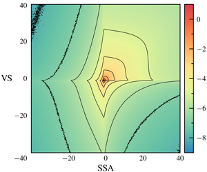
Figure 2. DNS results for the joint PDF of SSA and VS at filter scales (a)  $r/\unicode[STIX]{x1D702}=0$, (b)
  $r/\unicode[STIX]{x1D702}=50$, (c)
  $r/\unicode[STIX]{x1D702}=200$. Here,
  $\unicode[STIX]{x1D709}_{1}$ and
  $\unicode[STIX]{x1D709}_{2}$ are the fixed phase-space coordinates conjugate to the fluctuating quantities
  $(\widetilde{\unicode[STIX]{x1D64E}}\boldsymbol{\cdot }\widetilde{\unicode[STIX]{x1D64E}})\boldsymbol{ : }\widetilde{\unicode[STIX]{x1D64E}}$ and
  $\widetilde{\unicode[STIX]{x1D74E}}\widetilde{\unicode[STIX]{x1D74E}}\boldsymbol{ : }\widetilde{\unicode[STIX]{x1D64E}}$, respectively, while
  $\unicode[STIX]{x1D707}_{1}\equiv \langle (\widetilde{\unicode[STIX]{x1D64E}}\boldsymbol{\cdot }\widetilde{\unicode[STIX]{x1D64E}})\boldsymbol{ : }\widetilde{\unicode[STIX]{x1D64E}}\rangle$ and
  $\unicode[STIX]{x1D707}_{2}\equiv \langle \widetilde{\unicode[STIX]{x1D74E}}\widetilde{\unicode[STIX]{x1D74E}}\boldsymbol{ : }\widetilde{\unicode[STIX]{x1D64E}}\rangle$. The colours correspond to the values of the PDF, and the lines are isocontours of
  $\log _{10}$ PDF, shown in increments of 1.
In figure 1(b) we show the DNS data for the eigenframe contributions to  $\mathscr{L}\langle \sum _{i}\widetilde{\unicode[STIX]{x1D706}}_{i}^{3}\rangle$, where
  $(\widetilde{\unicode[STIX]{x1D64E}}\boldsymbol{\cdot }\widetilde{\unicode[STIX]{x1D64E}})\boldsymbol{ : }\widetilde{\unicode[STIX]{x1D64E}}=\sum _{i}\widetilde{\unicode[STIX]{x1D706}}_{i}^{3}$, and the results show that the
  $i=3$ contribution dominates and is the sole cause of the negativity of
  $\mathscr{L}\langle \sum _{i}\widetilde{\unicode[STIX]{x1D706}}_{i}^{3}\rangle$ at all scales in the flow. This shows that the SSA process that dominates the energy cascade is itself governed by compressional straining motions at all scales. In figure 1(c) we plot the eigenframe contributions to
  $\mathscr{L}\langle \sum _{i}\widetilde{{\mathcal{W}}}_{i}\rangle$, where
  $\widetilde{\unicode[STIX]{x1D74E}}\widetilde{\unicode[STIX]{x1D74E}}\boldsymbol{ : }\widetilde{\unicode[STIX]{x1D64E}}=\sum _{i}\Vert \widetilde{\unicode[STIX]{x1D74E}}\Vert ^{2}\widetilde{\unicode[STIX]{x1D706}}_{i}\cos ^{2}(\widetilde{\unicode[STIX]{x1D74E}},\widetilde{\boldsymbol{e}}_{i})\equiv \sum _{i}\widetilde{{\mathcal{W}}}_{i}$, and the results show that the contribution from
  $i=1$ is the most positive at all scales.
This is consistent with the results in Doan et al. (Reference Doan, Swaminathan, Davidson and Tanahashi2018) that show that at all scales in the flow, VS is dominated by the contribution from the extensional eigenvalue. Interestingly, while our results show  $\langle \widetilde{{\mathcal{W}}}_{1}\rangle >\langle \widetilde{{\mathcal{W}}}_{2}\rangle$ in the dissipation range (as observed in Gulitski et al. Reference Gulitski, Kholmyansky, Kinzelbach, Lüthi, Tsinober and Yorish2007),
  $\langle \widetilde{{\mathcal{W}}}_{1}\rangle \gg \langle \widetilde{{\mathcal{W}}}_{2}\rangle$ in the inertial range. While
  $\widetilde{{\mathcal{W}}}_{1}$ and
  $\widetilde{{\mathcal{W}}}_{3}$ have fixed signs, the sign of
  $\widetilde{{\mathcal{W}}}_{2}$ fluctuates, and as a result, the contribution to
  $\sum _{i}\langle \widetilde{{\mathcal{W}}}_{i}\rangle$ from
  $\langle \widetilde{{\mathcal{W}}}_{2}\rangle$ may be smaller than that from
  $\langle \widetilde{{\mathcal{W}}}_{1}\rangle$ due to partial cancellation of positive and negative
  $\widetilde{{\mathcal{W}}}_{2}$ in its average. To explore this, we computed
  $\langle |\widetilde{{\mathcal{W}}}_{2}|\rangle$ and found that at all scales,
  $\langle \widetilde{{\mathcal{W}}}_{2}\rangle <\langle |\widetilde{{\mathcal{W}}}_{2}|\rangle <\langle \widetilde{{\mathcal{W}}}_{1}\rangle$, such that the dominance of the
  $i=1$ contribution to
  $\sum _{i}\langle \widetilde{{\mathcal{W}}}_{i}\rangle$ is not simply caused by the fluctuating sign of
  $\widetilde{{\mathcal{W}}}_{2}$. It is mainly because
  $\widetilde{\unicode[STIX]{x1D706}}_{1}$ tends to be larger than
  $|\widetilde{\unicode[STIX]{x1D706}}_{2}|$, so that
  $\langle \widetilde{{\mathcal{W}}}_{1}\rangle$ dominates
  $\sum _{i}\langle \widetilde{{\mathcal{W}}}_{i}\rangle$, despite the fact that
  $\widetilde{\unicode[STIX]{x1D74E}}$ preferentially aligns with
  $\widetilde{\boldsymbol{e}}_{2}$ at all scales in the flow (Danish & Meneveau Reference Danish and Meneveau2018).
In figure 2 we show results for the joint PDF of VS and SSA at different filtering scales. The shape of the PDF contours are similar to those in the experimental work of Gulitski et al. (Reference Gulitski, Kholmyansky, Kinzelbach, Lüthi, Tsinober and Yorish2007) (they only considered the unfiltered case), showing the distinctive ‘corners’ of the contour lines along  $\unicode[STIX]{x1D709}_{1}/\unicode[STIX]{x1D707}_{1}=0$ and
  $\unicode[STIX]{x1D709}_{2}/\unicode[STIX]{x1D707}_{2}=0$. In figure 3(a) we show results for the PDFs of SSA and VS at different filtering scales. Concerning the
  $r/\unicode[STIX]{x1D702}=0$ results, in agreement with Gulitski et al. (Reference Gulitski, Kholmyansky, Kinzelbach, Lüthi, Tsinober and Yorish2007) we find that for
  $\unicode[STIX]{x1D709}/\unicode[STIX]{x1D707}>0$ the PDFs are similar; however, in disagreement with their results, we find that the PDFs for
  $\unicode[STIX]{x1D709}/\unicode[STIX]{x1D707}<0$ are quite different. The difference between the PDFs becomes larger for the filtered case
  $r/\unicode[STIX]{x1D702}=200$, for both
  $\unicode[STIX]{x1D709}/\unicode[STIX]{x1D707}<0$ and
  $\unicode[STIX]{x1D709}/\unicode[STIX]{x1D707}>0$. These results provide further support for our earlier assertions that the roles of SSA and VS must not be conflated. Not only are they dynamically very different, but furthermore, as figure 3(a) shows, the general statistics of the two processes are significantly different, despite the fact that their mean values are closely related through (2.7). This point is made even clearer in figure 3(b), where we show results for the correlation coefficient of VS and SSA,
  $\unicode[STIX]{x1D70C}_{VS,SSA}$. While
  $\unicode[STIX]{x1D70C}_{VS,SSA}$ is moderate in the dissipation range, in the inertial range
  $\unicode[STIX]{x1D70C}_{VS,SSA}$ approaches 0.3, indicating a weak correlation.

Figure 3. DNS results for (a) the PDF of  $\unicode[STIX]{x1D709}_{\unicode[STIX]{x1D6FC}}$, normalized by the mean value
  $\unicode[STIX]{x1D707}_{\unicode[STIX]{x1D6FC}}$ with
  $\unicode[STIX]{x1D6FC}=1,2$ (see the caption of figure 2 for the definitions of
  $\unicode[STIX]{x1D709}_{1},\unicode[STIX]{x1D709}_{2},\unicode[STIX]{x1D707}_{1},\unicode[STIX]{x1D707}_{2}$), and at different filter scales
  $r/\unicode[STIX]{x1D702}$, and (b) the correlation coefficient of VS and SSA,
  $\unicode[STIX]{x1D70C}_{VS,SSA}$, as a function of filter scale. Panel (c) shows results for
  $\unicode[STIX]{x1D701}_{n}\equiv \langle [(-3/4)\widetilde{\unicode[STIX]{x1D74E}}\widetilde{\unicode[STIX]{x1D74E}}\boldsymbol{ : }\widetilde{\unicode[STIX]{x1D64E}}]^{n}\rangle /\langle [(\widetilde{\unicode[STIX]{x1D64E}}\boldsymbol{\cdot }\widetilde{\unicode[STIX]{x1D64E}})\boldsymbol{ : }\widetilde{\unicode[STIX]{x1D64E}}]^{n}\rangle$ as a function of
  $r/\unicode[STIX]{x1D702}$, and for various
  $n$. The shaded regions around the lines denote the region bounded by the error bars (see appendix B for details).
Finally, we have argued that concerning the average energy cascade, the contribution from SSA is much larger than that from VS. However, it is important to consider whether the same holds true for fluctuations of the energy cascade about its average behaviour. To gain insight into this we consider the quantity
 $$\begin{eqnarray}\unicode[STIX]{x1D701}_{n}(r)\equiv \frac{\langle [(-3/4)\widetilde{\unicode[STIX]{x1D74E}}\widetilde{\unicode[STIX]{x1D74E}}\boldsymbol{ : }\widetilde{\unicode[STIX]{x1D64E}}]^{n}\rangle }{\langle [(\widetilde{\unicode[STIX]{x1D64E}}\boldsymbol{\cdot }\widetilde{\unicode[STIX]{x1D64E}})\boldsymbol{ : }\widetilde{\unicode[STIX]{x1D64E}}]^{n}\rangle }.\end{eqnarray}$$
 The results for  $\unicode[STIX]{x1D701}_{n}$ are shown in figure 3(c) for different
  $n$ and filtering scales
  $r/\unicode[STIX]{x1D702}$. For
  $n=1$, equation (2.7) gives
  $\unicode[STIX]{x1D701}_{1}=1$, as observed in our numerical results for each
  $r/\unicode[STIX]{x1D702}$. However, for
  $n>1$,
  $\unicode[STIX]{x1D701}_{n}>1$ at each scale, and reaches values
  $O(10)$ for
  $n=4$, implying that VS may play a leading-order role during strong fluctuations of the energy cascade about its average value. This increasingly important role of VS compared with SSA during large fluctuations of the energy cascade about the average behaviour may in part be associated with the known fact that the vorticity field is more intermittent that the strain-rate field in turbulent flows (Chen, Sreenivasan & Nelkin Reference Chen, Sreenivasan and Nelkin1997; Donzis, Yeung & Sreenivasan Reference Donzis, Yeung and Sreenivasan2008; Buaria et al. Reference Buaria, Pumir, Bodenschatz and Yeung2019).
In closing this section we note that for a more complete understanding of fluctuations of the energy cascade in turbulence one must also consider the role played by subgrid stresses (Buzzicotti et al. Reference Buzzicotti, Linkmann, Aluie, Biferale, Brasseur and Meneveau2018). These subgrid stresses interact with the filtered fields  $\widetilde{\unicode[STIX]{x1D64E}}$ and
  $\widetilde{\unicode[STIX]{x1D74E}}$, and make a contribution to the energy cascade. Such an investigation will be pursued in future work.
4 Conclusions
We have presented theoretical and numerical results showing that vortex stretching is not the main mechanism driving the average energy cascade in isotropic turbulence. Instead, the main mechanism driving the average cascade is the strain self-amplification process, which is a fundamentally distinct dynamical process from that of vortex stretching. However, our numerical results imply that vortex stretching may play a stronger role during fluctuations of the cascade about its average behaviour, which may be associated with the known fact that the vorticity field is more intermittent than the strain-rate field in turbulence.
Acknowledgements
We thank G. Katul, A. Porporato and M. Iovieno for stimulating discussions. This work used the Extreme Science and Engineering Discovery Environment (XSEDE), supported by National Science Foundation grant ACI-1548562 (Towns et al. Reference Towns, Cockerill, Dahan, Foster, Gaither, Grimshaw, Hazlewood, Lathrop, Lifka and Peterson2014).
Declaration of interests
The authors report no conflict of interest.
Appendix A
Here we give details of the steps in the analysis leading to (2.3), using the same notation as in the paper, and our method to avoid this compressibility issue discussed in § 2.
We first define  $\widetilde{\boldsymbol{u}}(\boldsymbol{x},t)\equiv \int _{\mathbb{R}^{3}}{\mathcal{G}}_{\ell }(\Vert \boldsymbol{y}\Vert )\boldsymbol{u}(\boldsymbol{x}-\boldsymbol{y},t)\,\text{d}\boldsymbol{y}$, where the filtering length scale
  $\ell$ is for now an independent variable. We then denote an incompressible filtered fluid velocity increment by
  $\unicode[STIX]{x0394}^{\ast }\widetilde{\boldsymbol{u}}(\boldsymbol{x},\boldsymbol{r},\ell ,t)$, which satisfies
 $$\begin{eqnarray}\displaystyle & \boldsymbol{\unicode[STIX]{x2202}}_{\boldsymbol{r}}\boldsymbol{\cdot }\unicode[STIX]{x0394}^{\ast }\widetilde{\boldsymbol{u}}(\boldsymbol{x},\boldsymbol{r},\ell ,t)|_{\boldsymbol{x}}=0, & \displaystyle\end{eqnarray}$$
 $$\begin{eqnarray}\displaystyle & \unicode[STIX]{x0394}^{\ast }\widetilde{\boldsymbol{u}}(\boldsymbol{x},\boldsymbol{r},\ell ,t)|_{\ell }=\unicode[STIX]{x0394}\widetilde{\boldsymbol{u}}(\boldsymbol{x},\boldsymbol{r},\ell ,t). & \displaystyle\end{eqnarray}$$
The formal solution of (A 1) can be expressed as
 $$\begin{eqnarray}\unicode[STIX]{x0394}^{\ast }\widetilde{\boldsymbol{u}}(\boldsymbol{x},\boldsymbol{r},\ell ,t)=\boldsymbol{\unicode[STIX]{x2202}}_{\boldsymbol{ r}}\times \widetilde{\boldsymbol{{\mathcal{A}}}}^{\ast }(\boldsymbol{x},\boldsymbol{r},\ell ,t)|_{\boldsymbol{ x}},\end{eqnarray}$$
 where  $\widetilde{\boldsymbol{{\mathcal{A}}}}^{\ast }$ is a vector potential of the incompressible increment. Substituting (A 3) into (A 2) an equation for the vector potential is obtained,
 $$\begin{eqnarray}\boldsymbol{\unicode[STIX]{x2202}}_{\boldsymbol{r}}\times \widetilde{\boldsymbol{{\mathcal{A}}}}^{\ast }(\boldsymbol{x},\boldsymbol{r},\ell ,t)|_{\boldsymbol{ x},\ell }=\unicode[STIX]{x0394}\widetilde{\boldsymbol{u}}(\boldsymbol{x},\boldsymbol{r},\ell ,t).\end{eqnarray}$$
 This now clarifies the notation used in (A 2);  $\unicode[STIX]{x0394}^{\ast }\widetilde{\boldsymbol{u}}(\boldsymbol{x},\boldsymbol{r},\ell ,t)|_{\ell }$ means that when, according to the vector potential expression for
  $\unicode[STIX]{x0394}^{\ast }\widetilde{\boldsymbol{u}}$, the curl operator
  $\boldsymbol{\unicode[STIX]{x2202}}_{\boldsymbol{r}}\times \{\cdot \}$ acts on
  $\widetilde{\boldsymbol{{\mathcal{A}}}}^{\ast }$,
  $\ell$ is to be held fixed – that is,
  $\unicode[STIX]{x0394}^{\ast }\widetilde{\boldsymbol{u}}=\unicode[STIX]{x0394}\widetilde{\boldsymbol{u}}$ when
  $\ell$ does not depend on
  $r$. The solution of (A 4) reads
 $$\begin{eqnarray}\widetilde{\boldsymbol{{\mathcal{A}}}}^{\ast }(\boldsymbol{x},\boldsymbol{r},\ell ,t)=2\widetilde{\boldsymbol{{\mathcal{A}}}}(\boldsymbol{x}+\boldsymbol{r}/2,\ell ,t)+2\widetilde{\boldsymbol{{\mathcal{A}}}}(\boldsymbol{x}-\boldsymbol{r}/2,\ell ,t)+\widetilde{\boldsymbol{{\mathcal{B}}}}(\boldsymbol{x},\ell ,t),\end{eqnarray}$$
 where  $\widetilde{\boldsymbol{{\mathcal{A}}}}$ is a vector potential associated with the velocity field filtered at length
  $\ell$, defined through
  $\widetilde{\boldsymbol{u}}(\boldsymbol{x},\ell ,t)=\unicode[STIX]{x1D735}\times \widetilde{\boldsymbol{{\mathcal{A}}}}(\boldsymbol{x},\ell ,t)|_{\ell }$. Here
  $\widetilde{\boldsymbol{{\mathcal{B}}}}(\boldsymbol{x},\ell ,t)$ is an integration constant, since (A 4) has been integrated in
  $\boldsymbol{r}$ at fixed
  $\boldsymbol{x}$ and
  $\ell$. Using (A 5) into (A 3) we then obtain the expression for the incompressible filtered velocity increment, equation (2.2).
In order to relate  $\unicode[STIX]{x0394}^{\ast }\widetilde{\boldsymbol{u}}(\boldsymbol{x},\boldsymbol{r},\ell ,t)$ to the velocity gradient filtered at scale
  $r$, namely
  $\widetilde{\unicode[STIX]{x1D71E}}\equiv \unicode[STIX]{x1D735}\widetilde{\boldsymbol{u}}$, we choose
  $\ell =r$ and Taylor expand the terms involving
  $\widetilde{\boldsymbol{{\mathcal{A}}}}$ in (2.2) in the variable
  $\boldsymbol{r}$, explicitly retaining terms up to second order,
 $$\begin{eqnarray}\widetilde{\boldsymbol{{\mathcal{A}}}}(\boldsymbol{x}+\boldsymbol{r}/2,r,t)+\widetilde{\boldsymbol{{\mathcal{A}}}}(\boldsymbol{x}-\boldsymbol{r}/2,r,t)=2\widetilde{\boldsymbol{{\mathcal{A}}}}(\boldsymbol{x},r,t)+{\textstyle \frac{1}{4}}(\boldsymbol{r}\boldsymbol{r}\boldsymbol{ : }\unicode[STIX]{x1D735}\unicode[STIX]{x1D735})\widetilde{\boldsymbol{{\mathcal{A}}}}(\boldsymbol{x},r,t)+\boldsymbol{h},\end{eqnarray}$$
 where  $\boldsymbol{h}(\boldsymbol{x},\boldsymbol{r},t)$ denotes the remainder term, defined (since the expansion may be only asymptotic) as the difference between the left-hand side and the first two terms on the right-hand side of (A 6). This remainder term will be subleading due to the smoothness of
  $\widetilde{\boldsymbol{{\mathcal{A}}}}$ on scales
  ${\leqslant}O(r)$.
Substituting (A 6) into (A 3) yields
 $$\begin{eqnarray}\unicode[STIX]{x0394}^{\ast }\widetilde{\boldsymbol{u}}=\widetilde{\unicode[STIX]{x1D71E}}\boldsymbol{\cdot }\boldsymbol{r}+\frac{\boldsymbol{r}}{r}\times \left[\frac{1}{2}(\boldsymbol{r}\boldsymbol{r}\boldsymbol{ : }\unicode[STIX]{x1D735}\unicode[STIX]{x1D735})\unicode[STIX]{x2202}_{r}\widetilde{\boldsymbol{{\mathcal{A}}}}+\unicode[STIX]{x2202}_{r}(4\widetilde{\boldsymbol{{\mathcal{A}}}}+\widetilde{\boldsymbol{{\mathcal{B}}}})\right]+2\boldsymbol{\unicode[STIX]{x2202}}_{\boldsymbol{r}}\times \boldsymbol{h},\end{eqnarray}$$
 where  $\widetilde{\unicode[STIX]{x1D71E}}=\widetilde{\unicode[STIX]{x1D71E}}(\boldsymbol{x},r,t)$,
  $\widetilde{\boldsymbol{{\mathcal{A}}}}=\widetilde{\boldsymbol{{\mathcal{A}}}}(\boldsymbol{x},r,t)$ and
  $\widetilde{\boldsymbol{{\mathcal{B}}}}=\widetilde{\boldsymbol{{\mathcal{B}}}}(\boldsymbol{x},r,t)$. In the paper the dependence upon
  $r$ due to the filtering is implicitly indicated by the tilde. The cross product term in (A 7) represents the ‘compressible correction’ that captures the effect of the variable filtering length on the velocity increment, and guarantees
  $\boldsymbol{\unicode[STIX]{x2202}}_{\boldsymbol{r}}\boldsymbol{\cdot }\unicode[STIX]{x0394}^{\ast }\widetilde{\boldsymbol{u}}(\boldsymbol{x},\boldsymbol{r},\ell ,t)=0~\forall \ell (r)$. Since this term lies in the plane orthogonal to
  $\boldsymbol{r}$, the longitudinal increments satisfy
  $\unicode[STIX]{x0394}^{\ast }\widetilde{u}_{\Vert }=\unicode[STIX]{x0394}\widetilde{u}_{\Vert }$, while the perpendicular increments differ,
  $\unicode[STIX]{x0394}^{\ast }\widetilde{u}_{\bot }\neq \unicode[STIX]{x0394}\widetilde{u}_{\bot }$.
Once the incompressible filtered velocity increment is defined, the nonlinear energy flux is expressed using the decomposition  $\unicode[STIX]{x0394}\boldsymbol{u}=\unicode[STIX]{x0394}^{\ast }\widetilde{\boldsymbol{u}}+\unicode[STIX]{x0394}^{\ast }\boldsymbol{u}^{\prime }$ and invoking isotropy
 $$\begin{eqnarray}\boldsymbol{\unicode[STIX]{x2202}}_{\boldsymbol{r}}\boldsymbol{\cdot }\boldsymbol{T}=\frac{1}{2}\left(\unicode[STIX]{x2202}_{r}+\frac{2}{r}\right)\langle \Vert \unicode[STIX]{x0394}^{\ast }\widetilde{\boldsymbol{u}}\Vert ^{2}\unicode[STIX]{x0394}^{\ast }\widetilde{u}_{\Vert }\rangle +F,\end{eqnarray}$$
 where  $F(r)$ denotes the contributions involving the subgrid field
  $\unicode[STIX]{x0394}^{\ast }\boldsymbol{u}^{\prime }$. Because of isotropy, the quantity
  $\langle \Vert \unicode[STIX]{x0394}^{\ast }\widetilde{\boldsymbol{u}}\Vert ^{2}\unicode[STIX]{x0394}^{\ast }\widetilde{u}_{\Vert }\rangle$ is physically related to the invariant
  $\langle (\widetilde{\unicode[STIX]{x1D71E}}^{\top }\!\boldsymbol{\cdot }\widetilde{\unicode[STIX]{x1D71E}})\boldsymbol{ : }\widetilde{\unicode[STIX]{x1D71E}}\rangle$, which is then employed to express the third-order structure functions
 $$\begin{eqnarray}\displaystyle & \langle \unicode[STIX]{x0394}^{\ast }\widetilde{u}_{\Vert }^{3}\rangle ={\textstyle \frac{2}{35}}\langle (\widetilde{\unicode[STIX]{x1D71E}}^{\top }\boldsymbol{\cdot }\widetilde{\unicode[STIX]{x1D71E}})\boldsymbol{ : }\widetilde{\unicode[STIX]{x1D71E}}\rangle r^{3}+{\mathcal{H}}_{\Vert }, & \displaystyle\end{eqnarray}$$
 $$\begin{eqnarray}\displaystyle & \langle \unicode[STIX]{x0394}^{\ast }\widetilde{u}_{\Vert }\unicode[STIX]{x0394}^{\ast }\widetilde{u}_{\bot }^{2}\rangle ={\textstyle \frac{4}{105}}\langle (\widetilde{\unicode[STIX]{x1D71E}}^{\top }\boldsymbol{\cdot }\widetilde{\unicode[STIX]{x1D71E}})\boldsymbol{ : }\widetilde{\unicode[STIX]{x1D71E}}\rangle r^{3}+C+{\mathcal{H}}_{\bot }, & \displaystyle\end{eqnarray}$$
 where  ${\mathcal{H}}_{\Vert }$ and
  ${\mathcal{H}}_{\bot }$ denote the contributions arising from
  $\boldsymbol{h}$ in (A 7). Here
  $C(r)$ denotes the contribution arising from the compressibility correction term in (A 7), which is determined by incompressibility and isotropy of the flow. Indeed, as shown by Hill (Reference Hill1997),
 $$\begin{eqnarray}\langle \unicode[STIX]{x0394}u_{\Vert }\unicode[STIX]{x0394}u_{\bot }^{2}\rangle ={\textstyle \frac{1}{6}}\unicode[STIX]{x2202}_{r}(r\langle \unicode[STIX]{x0394}u_{\Vert }^{3}\rangle )\end{eqnarray}$$
and requiring that (A 11) is satisfied by the incompressible increment, using (A 9) which is free of compressibility effects, gives
 $$\begin{eqnarray}\langle \unicode[STIX]{x0394}^{\ast }\widetilde{u}_{\Vert }\unicode[STIX]{x0394}^{\ast }\widetilde{u}_{\bot }^{2}\rangle ={\textstyle \frac{1}{105}}\unicode[STIX]{x2202}_{r}(\langle (\widetilde{\unicode[STIX]{x1D71E}}^{\top }\boldsymbol{\cdot }\widetilde{\unicode[STIX]{x1D71E}})\boldsymbol{ : }\widetilde{\unicode[STIX]{x1D71E}}\rangle r^{4}+r{\mathcal{H}}_{\Vert }).\end{eqnarray}$$
 Substituting (A 9) and (A 12) into (A 8), we finally obtain (2.3), wherein  ${\mathcal{F}}$ is the sum of
  $F$ and the contributions from
  ${\mathcal{H}}_{\Vert }$.
Appendix B
In this appendix, we briefly describe the method used to construct the error bars in figure 3(c), which are important to consider for the high-order moments shown in that plot.
Let  $f(\boldsymbol{x},t)$ be an arbitrary random field; for a statistically stationary, homogeneous flow we may approximate the ensemble average
  $\langle f\rangle$ by a space-time averaging operator
 $$\begin{eqnarray}\displaystyle & \displaystyle \langle f\rangle \approx \overline{f^{\ast }}\equiv \frac{1}{T}\int _{0}^{T}f^{\ast }\,\text{d}t, & \displaystyle\end{eqnarray}$$
 $$\begin{eqnarray}\displaystyle & \displaystyle f^{\ast }\equiv \frac{1}{|\unicode[STIX]{x1D6FA}|}\int f\,\text{d}\boldsymbol{x}, & \displaystyle\end{eqnarray}$$
 where  $|\unicode[STIX]{x1D6FA}|$ is the measure of the domain in which the flow is taking place. In our simulations,
  $|\unicode[STIX]{x1D6FA}|$ is fixed and finite; however, assuming ergodicity, then we expect
  $\lim _{T\rightarrow \infty }\overline{f^{\ast }}\rightarrow \langle f\rangle$. In contrast, in our simulations,
  $T$ is finite, and it is therefore important to consider convergence errors in our estimation associated with the finitude of
  $T$.
$T$.
In order to define the convergence error, we introduce the finite mean  $\unicode[STIX]{x1D707}$ and variance
  $\unicode[STIX]{x1D70E}^{2}$ of the time series
  $f^{\ast }(t)$, and define its partial average as
 $$\begin{eqnarray}\overline{f^{\ast }}(\unicode[STIX]{x1D70F})\equiv \frac{1}{\unicode[STIX]{x1D70F}}\int _{0}^{\unicode[STIX]{x1D70F}}f^{\ast }(t)\,\text{d}t.\end{eqnarray}$$
 The deviation of the partial average from the exact mean,  $e(\unicode[STIX]{x1D70F})\equiv (\overline{f^{\ast }}(\unicode[STIX]{x1D70F})-\unicode[STIX]{x1D707})^{2}$, is employed to define the convergence error
 $$\begin{eqnarray}\unicode[STIX]{x1D716}(T)\equiv \sqrt{\frac{1}{T}\int _{0}^{T}e(\unicode[STIX]{x1D70F})\,\text{d}\unicode[STIX]{x1D70F}}.\end{eqnarray}$$
 The error defined in (B 4) measures the fluctuations of the partial average with respect to the ensemble average over the whole time window. Also, this convergence error  $\unicode[STIX]{x1D716}(T)$ vanishes for
  $T\rightarrow \infty$, when the time average is expected to approach the ensemble average. Indeed, with
  $\unicode[STIX]{x1D716}(T)\equiv \sqrt{F(T)/T}$, the fundamental theorem of calculus, together with the convergence of the partial averages to the ensemble average, implies
 $$\begin{eqnarray}\text{d}_{T}F(T)=o(1)\quad \text{for}~T\rightarrow \infty ,\end{eqnarray}$$
 and, if  $e$ is smooth (which it is for the quantities we are considering), then
  $F$ is even smoother so that equation (B 5) can be integrated yielding
  $F(T)=o(T)$ for
  $T\rightarrow \infty$. As a consequence, the error defined in (B 4) vanishes when the partial average converges to the ensemble average,
  $\lim _{T\rightarrow \infty }\unicode[STIX]{x1D716}(T)=\lim _{T\rightarrow \infty }\sqrt{F(T)/T}=0$.
Now, in figure 3(c) we plot the quantity  $\unicode[STIX]{x1D701}_{n}(r)$, defined in (3.1). Let us now introduce the quantity
  $\unicode[STIX]{x1D70E}_{n}(r,\unicode[STIX]{x1D70F})$, which is the same as
  $\unicode[STIX]{x1D701}_{n}(r)$, but with the ensemble averages in the definition of
  $\unicode[STIX]{x1D701}_{n}(r)$ replaced with a space average over the domain plus a time average over the interval
  $[0,\unicode[STIX]{x1D70F}]$. As before, we expect
  $\lim _{\unicode[STIX]{x1D70F}\rightarrow \infty }\unicode[STIX]{x1D70E}_{n}(r,\unicode[STIX]{x1D70F})\rightarrow \unicode[STIX]{x1D701}_{n}(r)$. In the DNS data, we have
  $\unicode[STIX]{x1D70F}\leqslant 6\unicode[STIX]{x1D70F}_{I}$, where
  $\unicode[STIX]{x1D70F}_{I}$ is the integral time scale of the flow. We may then estimate the convergence error using an approximation for
  $\unicode[STIX]{x1D716}(T)$ evaluated at
  $T=6\unicode[STIX]{x1D70F}_{I}$,
 $$\begin{eqnarray}\tilde{\unicode[STIX]{x1D716}}(r,6\unicode[STIX]{x1D70F}_{I})=\sqrt{\frac{1}{6\unicode[STIX]{x1D70F}_{I}}\int _{0}^{6\unicode[STIX]{x1D70F}_{I}}(\unicode[STIX]{x1D70E}_{n}(r,\unicode[STIX]{x1D70F})-\unicode[STIX]{x1D70E}_{n}(r,T=6\unicode[STIX]{x1D70F}_{I}))^{2}\,\text{d}\unicode[STIX]{x1D70F}},\end{eqnarray}$$
 since, by the Chebyshev inequality,  $\unicode[STIX]{x1D70E}_{n}(r,T=6\unicode[STIX]{x1D70F}_{I})$ is in probability the best estimate to
  $\unicode[STIX]{x1D701}_{n}(r)$. In figure 3(c) the error bars are constructed using
  $\tilde{\unicode[STIX]{x1D716}}(r,6\unicode[STIX]{x1D70F}_{I})$. Note that we use the estimate for the error in (B 6) since a direct estimation of the error by means of the Chebyshev inequality would be problematic due to the small number of time samples we have available (our DNS data consist of 19 snapshots of the flow).


