


1. Introduction
Passive control of flat plate boundary layers by means of miniature vortex generators (MVGs), which consist of pairs of winglets or rectangular blades arranged in spanwise oriented arrays, is of great practical interest because of their ability to delay the flow from transition to turbulence by effectively stabilising the Tollmien–Schlichting (TS) waves or attenuating the oblique disturbance waves so that skin friction drag reduction can be achieved (Fransson et al. Reference Fransson, Talamelli, Brandt and Cossu2006; Fransson & Talamelli Reference Fransson and Talamelli2012; Shahinfar, Sattarzadeh & Fransson Reference Shahinfar, Sattarzadeh and Fransson2014). The net drag reduction can be enhanced up to 65 % when the transition delay is sustained by placing a consecutive array of MVGs further downstream (Shahinfar et al. Reference Shahinfar, Sattarzadeh, Fransson and Talamelli2012; Sattarzadeh et al. Reference Sattarzadeh, Fransson, Talamelli and Fallenius2014). Numerous experimental and direct numerical simulation (DNS) studies of MVGs in flat plate laminar boundary layers yield a deeper understanding of the transition delay mechanism and the stability of laminar boundary layer controls (Siconolfi, Camarri & Fransson Reference Siconolfi, Camarri and Fransson2015a,Reference Siconolfi, Camarri and Franssonb). The capability of MVGs to generate streamwise vortices and, in turn, form long and stable streamwise evolving streaks by the lift-up mechanism is well understood (Landahl Reference Landahl1980). Fransson & Talamelli (Reference Fransson and Talamelli2012) explored the possibility of generating stable streamwise streaks to stabilise TS waves for transition delay. They reported that the maximum amplitude of stable streaks was approximately 30 % of the free-stream velocity, approximately double the value of that generated by circular roughness elements (Fransson et al. Reference Fransson, Brandt, Talamelli and Cossu2005), and the modulation effect was sustained for  $700h$ downstream of the MVGs (where
  $h$ is the blade height). Subsequently, Shahinfar et al. (Reference Shahinfar, Fransson, Sattarzadeh and Talamelli2013) conducted an extensive parametric study on TS wave stabilisation, utilising different MVG configurations and optimised the streak scaling and improved the streak amplitude definition by taking into consideration the spanwise periodicity of the streaks. Taking advantage of the high spatial resolution of DNS flow fields, Siconolfi et al. (Reference Siconolfi, Camarri and Fransson2015b) analysed flow instabilities introduced by MVGs, which may be one of the drawbacks of inadequate design of MVGs for transition delay, and may amplify the TS waves and lead to faster transitions (Sattarzadeh & Fransson Reference Sattarzadeh and Fransson2015).
In the context of flow separation control in adverse pressure gradient boundary layers, it has been shown that a MVG is capable of reducing separation by redirecting reverse flow (backflow) to the mean flow direction (see Lögdberg Reference Lögdberg2006). Experimentally, the flow dynamic of vortex generators in turbulent boundary layers (TBLs) has previously been investigated at relatively high Reynolds numbers (Lögdberg, Fransson & Alfredsson Reference Lögdberg, Fransson and Alfredsson2009). The authors were interested in the development of streamwise vortices introduced into the boundary layer by vortex generators, including the actual vortex propagation and vortex strength decay, and by using a potential flow model, they proposed a vortex-path model predicting the streamwise evolution of longitudinal vortices downstream of the vortex generators. However, that investigation does not provide further details about the interactions between MVG-induced flow features and the large-scale structures related to turbulent boundary layers.
The flat plate boundary layer studies by Fransson & Talamelli (Reference Fransson and Talamelli2012) and Shahinfar et al. (Reference Shahinfar, Fransson, Sattarzadeh and Talamelli2013) strongly suggest that the MVGs are able to impose large-scale vortical motions and generate long high- and low-speed streaks in the turbulent boundary layer by similar mechanisms. It would be interesting to investigate whether these streaks also persist in a turbulent boundary layer with moderate Reynolds numbers and how these streaks interact with turbulent coherent structures in the near-wall and outer regions. There is a lack of studies in the literature that have investigated the ability of MVGs to modify the small- and large-scale motions in turbulent boundary layers. The near-wall turbulence is well understood to be related to the formation of quasi-streamwise vortices and streamwise streaks by self-sustained mechanisms (Hamilton, Kim & Waleffe Reference Hamilton, Kim and Waleffe1995; Jiménez & Pinelli Reference Jiménez and Pinelli1999; Panton Reference Panton2001). Very large-scale motions or large-scale streamwise elongated modes have been found to exist far away from the wall, and they increasingly interfere with the near-wall turbulence with increasing Reynolds numbers (Hutchins & Marusic Reference Hutchins and Marusic2007b; Mathis, Hutchins & Marusic Reference Mathis, Hutchins and Marusic2009). Their distinctive inner and outer peaks are observed in both the streamwise and spanwise pre-multiplied streamwise velocity energy spectra at sufficiently high Reynolds numbers (Lee & Moser Reference Lee and Moser2015).
To the authors’ best knowledge, previous research has focused on laminar or transitional boundary layer flows, and there are limited studies that have investigated how MVGs influence the naturally occurring boundary layer turbulence, thus the complex interactions between the MVG array and these turbulent structures remain unclear. Here, a well-resolved large-eddy simulation of turbulent boundary layers mounted with a MVG array at moderate Reynolds numbers has been performed. We aim to investigate the flow dynamics underlying the MVG array and its relationship to the large- and small-scale motions. The work of Sattarzadeh & Fransson (Reference Sattarzadeh and Fransson2015) has suggested that the angle of attack of MVG blades  $\theta$ plays a significant role, reporting that the amplitude of the streaks is shown to grow with increasing
  $\theta$, but the streaks are subject to more severe instability if
  $\theta$ exceeds a certain threshold. Other decisive parameters are the blade height
  $(h)$, the distance between MVG blades
  $(d)$ and also the distance between MVG pairs
  $(\varLambda _z)$. We here keep the MVG parameters similar to the base configuration used by Shahinfar et al. (Reference Shahinfar, Fransson, Sattarzadeh and Talamelli2013) (i.e. the geometrical aspect ratios of MVGs). The present study also serves as a numerical investigation of these MVG parameters in a turbulent boundary layer. The remainder of this paper is organised as follows. In § 2 we first introduce the numerical code and the numerical MVG parameters. In § 3 we analyse and discuss the influences of MVGs on the mean flow statistics and turbulence properties of turbulent boundary layers. Further, we employ a triple decomposition of the velocity fluctuations, the pre-multiplied streamwise velocity energy spectra are computed and the modifications of the coherent motions are presented.
2. Numerical procedures and MVG configuration
A well-resolved large-eddy simulation is performed using a fully spectral numerical code (Chevalier, Lundbladh & Henningson Reference Chevalier, Lundbladh and Henningson2007) and two-dimensional parallelisation (Li, Schlatter & Henningson Reference Li, Schlatter and Henningson2008). A sub-grid-scale approximate deconvolution model is employed to compute approximations to the unfiltered solutions of the incompressible continuity and Navier–Stokes equations by a repeated filter operation (Schlatter, Stolz & Kleiser Reference Schlatter, Stolz and Kleiser2004),
 \begin{gather} \frac{\partial \hat{u}_i}{\partial x_i} = 0, \end{gather}
 \begin{gather}\frac{\partial \hat{u}_i}{\partial t} + \hat{u}_j \frac{\partial \hat{u}_i}{\partial x_j} + \frac{\partial \hat{p}}{\partial x_i} - \frac{1}{Re}\frac{\partial^2 \hat{u}_i}{\partial x_j \partial x_j} ={-}\chi H_N \circledast \hat{u}_i, \end{gather}
where superscripts  $\wedge$ refer to a resolved scale,
  $\circledast$ denotes the convolution and the relaxation term
  ${-\chi H_N \circledast \hat {u}_i} : \chi$ is the model coefficient;
  $H_N \circledast \hat {u}_i$ are the high-pass approximately deconvolved quantities (Stolz, Adams & Kleiser Reference Stolz, Adams and Kleiser2001; Schlatter et al. Reference Schlatter, Stolz and Kleiser2004, Reference Schlatter, Li, Brethouwer, Johansson and Henningson2010; Eitel-Amor, Örlü & Schlatter Reference Eitel-Amor, Örlü and Schlatter2014). The Reynolds number is defined as
  $Re = U_\infty \delta^*_0/\nu$, where
  $U_\infty$ is the free stream velocity,
  $\delta^*_0$ is the inlet displacement thickness and
  $\nu$ is the kinematic viscosity. In the following, the coordinates
  $x_i$ and the corresponding velocity components
  $u_i$ are denoted as
  $x, y$ and
  $z$ with corresponding velocities
  $u, v$ and
  $w$ in the streamwise, wall-normal and spanwise directions, respectively. The spatial discretisation is based on a Fourier series with 3/2 zero padding for de-aliasing in the streamwise
  $(x)$ and spanwise
  $(z)$ directions, and a Chebyshev polynomial is employed in the wall-normal direction
  $(y)$. The time advancement is carried out by a second-order Crank–Nicolson scheme for the viscous terms and a third-order four-stage Runge–Kutta scheme for the nonlinear terms (Chevalier et al. Reference Chevalier, Lundbladh and Henningson2007).
The simulation of a turbulent boundary layer was carried out with a computational domain in the streamwise, wall-normal and spanwise directions, respectively:  $x_L \times y_L \times z_L = 6000 \delta _0^* \times 200 \delta _0^* \times 360 \delta _0^*$ using
  $6144 \times 513 \times 768$ spectral modes, giving uniform grid spacings of
  ${\rm \Delta} x^+ \approx 16.9$ and
  ${\rm \Delta} z^+ \approx 8.1$ in the streamwise and spanwise directions (the superscript
  $+$ refers to scaling with the viscous velocity
  $u_\tau = \sqrt {\tau _w/\rho }$, where
  $\tau _w$ is the wall shear stress and
  $\rho$ is the fluid density). In the wall-normal direction, there is a minimum of
  $15$ Chebyshev collocation points within the region
  $y^+ < 10$. The first grid point away from the wall is at
  $y^+ \approx 0.03$, and the maximum spacing is
  ${\rm \Delta} y_{{max}}^+ = 10.6$. Periodic boundary conditions are applied in the streamwise and spanwise directions, while a no-slip condition is applied at the wall with a Neumann condition applied at the free-stream boundary. A fringe region is employed at the end of the computational domain, and the flow is damped via a volume force to retain periodic boundary conditions in the streamwise direction. A low-amplitude volume force trip is applied to trigger the transition to turbulent flow at the inlet region (Schlatter & Örlü Reference Schlatter and Örlü2012).
In this study, we consider a rectangular-bladed MVG similar to those used by Lögdberg et al. (Reference Lögdberg, Fransson and Alfredsson2009), Sattarzadeh et al. (Reference Sattarzadeh, Fransson, Talamelli and Fallenius2014) and Sattarzadeh & Fransson (Reference Sattarzadeh and Fransson2015). The MVG geometry and configuration are shown in figure 1 $(a)$. A total of seven pairs of MVG was imposed via a volume forcing method (see Appendix A for details) (Brynjell-Rahkola et al. Reference Brynjell-Rahkola, Schlatter, Hanifi and Henningson2015; Canton et al. Reference Canton, Örlü, Chin and Schlatter2016; Chin et al. Reference Chin, Örlü, Monty, Hutchins, Ooi and Schlatter2017) and positioned at
  $x_{{M}}/\delta _0^* = 950$ from the inlet (corresponding to
  $Re_\tau = \delta ^+ \simeq 430$, where
  $\delta$ is the boundary layer thickness). The boundary layer conditions at
  $x = x_{M}$ are summarised in table 1. The MVG parameters are scaled by the inlet displacement thickness
  $\delta _0^*$. Here,
  $h = 4$ is the blade height,
  $t = 1$ is the blade thickness,
  $L_x = 10$ is the blade length,
  $\alpha = 15^\circ$ is the angle of attack of the MVG with respect to the flow direction,
  $d =10$ is the spanwise distance between the centroids of blades in one pair and
  $\varLambda _z = 40$ is the spanwise spacing between MVG pairs (see figure 1
 $a$). The geometrical ratios of MVG:
  ${L_x}/{h} = {d}/{h} = 2.5, {\varLambda _z}/{h} = 10$ and
  ${h}/{\delta ^*} = 1$ (where
  $\delta ^*$ is the displacement thickness) are similar to the base configuration used by Shahinfar et al. (Reference Shahinfar, Fransson, Sattarzadeh and Talamelli2013). In addition, the ratio of the MVG height to the boundary layer thickness is
  $h/\delta \simeq 0.19$, which is similar to those used by Lin (Reference Lin2002) and Lögdberg et al. (Reference Lögdberg, Fransson and Alfredsson2009). The time-averaged velocity and its fluctuation are denoted by
  $(\bar {\cdot })$ and a prime
  $(\cdot ')$, respectively, and the symbol
  $\langle \cdot \rangle$ denotes a spanwise-averaged quantity over one complete spanwise wavelength
  $\varLambda _z$. A capital letter denotes both the spanwise and temporally averaged quantity, e.g.
  $U(y) = \langle \bar {u} \rangle$. In the following, time-averaged quantities are further averaged in the periodic spanwise direction. The periodic spanwise coordinate is denoted as
  $z^\ast = {modulo}(z,\varLambda _z)$ within each MVG pair. The time-averaged statistics of the two pairs of MVG located at the two ends of the MVG array were not considered to avoid edge effects. The simulation was run for at least
  $Tu_\tau /\delta \approx 8$ eddy turnover times at
  $Re_\tau \simeq 1000$ before collecting data, and the time statistics are sampled for at least
  $Tu_\tau /\delta \approx 7$. The quality of the statistics was checked and validated by the Reynolds-averaged turbulent kinetic energy (TKE) transport (i.e. TKE-budget Pope Reference Pope2000) at
  $Re_\tau \simeq 1350$ with previous direct numerical simulation (DNS) TBL by Schlatter & Örlü (Reference Schlatter and Örlü2010), as shown in figure 2. The terms collapse well with the previous DNS TBL. The generation of the vortex pair by the present MVG configuration is illustrated in figure 1(b,c), where the time-averaged streamwise vorticity contours at initial (
 $x^\ast /h = 5$) and at further downstream positions (
 $x^\ast /h = 25$) are plotted (where
  $x^\ast = x-x_{M}$ is defined). The primary vortex pair (PVP) with opposite vorticity is scaled with the MVG height and decays downstream along the centre of the MVG pair. The secondary vortices induced by the PVP are observed below with opposite vorticity. Additionally, a volumetric view of time-averaged streamwise vorticity at
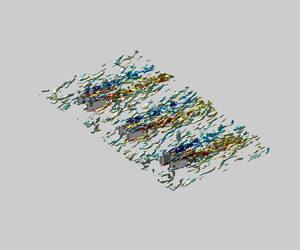
  $|\bar {\omega }_xh/U_\infty | = 0.03$ is presented in figure 3. The secondary vortices (opposite vorticity) near the wall are highlighted by lighter colours. The PVP is originated from the shear layer introduced by MVG and appears to be diffused and decayed downstream at
  $x^\ast /h \simeq 50$, presumably due to the lift-up effect where low-speed fluids are lifted at both sides of the PVP, and high-speed fluids are pushed towards the wall at the centre of the vortex pair (Fransson & Talamelli Reference Fransson and Talamelli2012), which creates alternating high- and low-speed streaks. Moving downstream, the low-speed streaks are reinforced by low-speed streaks originating from the adjacent MVG pairs (Lögdberg et al. Reference Lögdberg, Fransson and Alfredsson2009).

Figure 1.  $(a)$ Schematic diagram of the flow domain and the MVG configuration. (b,c) The time-averaged streamwise vorticity downstream of the MVG. Black contour lines outline the vorticity levels. The centre (point o in
  $(a)$) plane projection of MVG in the
  $y\text {--}z$ plane is outlined by a rectangular black box. The origin of
  $x^\ast = x-x_{M}$ is defined at the centre of the MVG.

Figure 2. The (——) TKE-budget (Pope Reference Pope2000) at  $x^\ast /h \simeq 1000\, (Re_\tau \simeq 1350)$. The arrow indicates budget terms in the order: dissipation, viscous diffusion, convection, velocity–pressure gradient, turbulent diffusion and production. Residuals are shown by coloured lines:
  $x^\ast /h = 25, 50, 500, 1000$ (blue, green, yellow and red). Black symbols indicate the data of DNS TBL at
  $Re_\tau \simeq 1270$ (Schlatter & Örlü Reference Schlatter and Örlü2010). The vertical dashed line denotes
  $y^+ = h^+$.

Figure 3. Isosurfaces of mean streamwise vorticity at  $|\bar {\omega }_xh/U_\infty | = 0.03$. Red for primary clockwise rotating vortices (
 $\bar {\omega }_xh/U_\infty = +0.03$) and blue for primary counter-clockwise rotating vortices (
 $\bar {\omega }_xh/U_\infty = -0.03$). Secondary (induced) vortices with opposite vorticity in close proximity to the wall are illustrated by the light colour versions (light red for
  $\bar {\omega }_xh/U_\infty = +0.03$ and light blue for
  $\bar {\omega }_xh/U_\infty = -0.03$).
Table 1. Smooth wall turbulent boundary layer conditions at the MVG location  $(x=x_M)$.
3. Results
3.1. Instantaneous streak patterns
The PVP induced by MVG (figure 3) leads to the formation of the high- and low-speed streaks by transporting the high- and low-momentum fluids through the lift-up mechanism, which has been reported in numerous studies performed in laminar boundary layers (e.g. Fransson & Talamelli Reference Fransson and Talamelli2012; Shahinfar et al. Reference Shahinfar, Fransson, Sattarzadeh and Talamelli2013). The instantaneous streak pattern around the MVG in a turbulent boundary layer is illustrated in figure 4 $(a)$. Upstream of the MVG (
 $x^\ast /h < 0$) are typically the naturally occurring large-scale structures associated with high- and low-momentum regions with self-similar spanwise length scales that vary with distance from the wall (Tomkins & Adrian Reference Tomkins and Adrian2003). Downstream of the MVG (
 $x^\ast /h > 0$) the flow patterns become more organised with high- and low-speed region spacings that are scaled with the spanwise distance (
 $\varLambda _z$) between the MVG pairs. A closer view is presented in figure 4
 $(b)$. The isosurfaces of vortical structures are computed using the
  $\lambda _2$-criterion (Jeong & Hussain Reference Jeong and Hussain1995) and coloured by the mean streamwise velocity. High-speed streaks are flanked by the low-speed streaks and vortical structures on both sides. The vortical structures are commonly observed slightly above and outwards of the low-speed streaks, reflecting ejection events associated with the lift-up mechanism. To quantitatively measure the streamwise streaks, the growth amplitude of the streamwise streaks is defined as
 \begin{equation} A_{ST}(x) = \frac{1}{U_\infty}\int_{-\varLambda_z/2}^{\varLambda_z/2} \int_{0}^{\delta} | \bar{u}(x,y,z^\ast)-U(x,y) |\,\textrm{d} {y}\,\textrm{d} {z^\ast},\end{equation}
which considers the spanwise periodicity of the streaks by integrating the MVG-induced fluctuation over one complete spanwise wavelength (Shahinfar et al. Reference Shahinfar, Fransson, Sattarzadeh and Talamelli2013). The MVG-induced-vortex strength is based on the integral of the squared streamwise vorticity (enstrophy) over one complete spanwise wavelength as
 \begin{equation} {\gamma} = \frac{h^2}{U_\infty^2}\int_{-\varLambda_z/2}^{\varLambda_z/2} \int_{0}^{\delta} \bar{\omega}_x^2(x,y,z^\ast) \,\textrm{d} {y}\,\textrm{d} {z^\ast}.\end{equation}
Figure 4.  $(a)$ Instantaneous visualisation of the high-speed (cyan) and low-speed (blue) streaks (
 $u'^+ = \pm 2.5$).
  $(b)$ Closer views of the instantaneous flow patterns of high-speed and low-speed streaks (same colour code as
  $(a)$). Vortical structures are detected by the
  $\lambda _2-{criterion}$ and coloured by the mean streamwise velocity.
Figure 5 $(a)$ shows the streak amplitude and induced-vortex strength based on (3.1) and (3.2) at
  $0 < x^\ast /h < 1000$, normalised by initial values at
  $x=x_M$. Based on these trends, the flow is split into three distinct regions. In the first region
  $(\text {I})$, where
  $5 < x^\ast /h < 50$, the vortex decreasing strength is coupled to the streak formation. The vortex strength decay follows a power-law relation of
  $\gamma /\gamma _{{M}} \sim (x^\ast /h)^{-1.1}$ for
  $5< x^\ast /h<50$ (blue line). The decay rate maybe different due to the definition used. Lögdberg et al. (Reference Lögdberg, Fransson and Alfredsson2009) reported the vortex circulation decays exponentially at a rate of
  $-0.0164$ with respect to the downstream distance, but the calculation considered was the vortex area enclosed by five per cent of the maximum value of the second invariant of the velocity gradient
  $(0.05{Q}_{max})$, which did not take into account the secondary (induced) effects. Figure 5(b,c) shows the streamwise evolution of the PVP in the first region
  $(\text {I})$, which is defined as the position at the local maximum of the absolute streamwise vorticity. The results qualitatively agree with those obtained by Lögdberg et al. (Reference Lögdberg, Fransson and Alfredsson2009). Overall, region I reflects the fact that energy is being redistributed from PVP to the streamwise velocity component (Shahinfar et al. Reference Shahinfar, Fransson, Sattarzadeh and Talamelli2013). At region
  $(\text {II})$, where
  $50< x^\ast /h<500$, the streak amplitude settles to a somewhat steady value of
  $A_{ST}/A_{ST,M} \simeq 7.5$. The stabilisation effect presumably results from the interactions of streaks generated between the MVG pairs, forming long and steady high- and low-speed regions. On the other hand, the vortex strength decreases steadily at a rate
  $\gamma /\gamma _{{M}} \sim (x^\ast /h)^{-0.1}$. Region (III) denotes the range
  $x^\ast /h > 500$, which is the onset of equilibrium. The streak amplitude decreases due to viscous dissipation (Shahinfar et al. Reference Shahinfar, Fransson, Sattarzadeh and Talamelli2013), and the mean flow and turbulent statistics are less dependent on the effect of MVGs and collapse to the smooth wall case, as shown in the following section.

Figure 5.  $(a)$ Streak amplitude
  $A_{ST}$ (black
  $\circ$) and vorticity strength
  $\gamma$ (red
  $\diamond$), normalised by the values at
  $x=x_{M}$. Blue solid line in region (I) approximates a power-law relation
  $\gamma /\gamma _{M} \sim (x^\ast /h)^{-1.1}$ for
  $5< x^\ast /h<50$, and solid green line within region (II) indicates
  $\gamma /\gamma _{M} \sim (x^\ast /h)^{-0.1}$. Streamwise evolution of vortex centre in
  $(b)$ side view and
  $(c)$ top view. Red for clockwise and blue for counter-clockwise rotation vortices. In
  $(b)$, the solid line represents the Reynolds number based on the displacement thickness and the dash-dotted line represents the Reynolds number based on the momentum thickness.
3.2. Mean flow characteristics
The mean streamwise and secondary flow topology are illustrated in figure 6 where the time-averaged streamwise velocity (contours) and cross-flow velocity (streamlines) are plotted at  $x^\ast /h =5, 25, 50$ and
  $500$. In the near-wake region
  $(x^\ast /h = 5)$, opposite secondary motion is observed close to the wall (indicated by the red arrow on figure 6
 $a$), which is induced by rotation of the PVP, and the PVP lift away from the wall and move apart along the downstream (figure 6
 $b\text {--}d$) due to self-induction (Lögdberg et al. Reference Lögdberg, Fransson and Alfredsson2009). The contour colours illustrate the mean streamwise velocity downstream in the
  $z\text {--}y$ cross-section views. The downwash motion induced by the PVP causes the high-momentum region to form between the MVG, while the low-momentum region is formed along the sides and interacts with the low-momentum region originating from the adjacent MVG pairs (Fransson & Talamelli Reference Fransson and Talamelli2012). The black contour lines at
  $\bar {u}=0.6U_\infty$ illustrate the development of regions along the spanwise direction and show the respective changes in the wall-normal direction. The mean flow exhibits an initial momentum deficit and a fast momentum recovery after the streaks have settled. The mean velocity deficit is estimated based on the mean velocity profile, as shown in figure 7. The flow exhibits an apparent velocity defect at
  $x^\ast /h =5$. The velocity defect in the mean flow profile can be estimated by comparing the downward shift of the log-law constants, as shown by the dash-dotted lines in figure 7. This yields
  ${\rm \Delta} U^+ = 2$ at
  $y/h \simeq 0.5$, corresponding to the half-blade height.

Figure 6. Mean streamwise velocity (colour contours) and secondary flow topology (streamlines) at the downstream of the MVG ( $a\text {--}d$):
  $x^\ast /h = 5,25,50$ and
  $500$.

Figure 7. Mean streamwise velocity. Downstream locations are at  $x^\ast /h \simeq 5$ (black
  $\circ$),
  $25$ (red
  $\circ$),
  $50$ (blue
  $\circ$) and
  $1000$ (purple
  $\circ$). Light blue dashed, dotted and solid lines represent smooth wall DNS TBL at
  $Re_\tau \simeq 500,1000$ and
  $2000$ (Chan, Schlatter & Chin Reference Chan, Schlatter and Chin2021), respectively. The thick grey line denotes
  $y^+ \simeq h^+$. Dash-dotted lines represent linear and log-law regions with
  $\kappa = 0.41$ and
  $C=3.2$ and
  $5.2$.
The velocity defect is known to be associated with skin friction drag. Locally, the skin friction is modulated over the high- and low-speed regions along the spanwise direction. On the upwash side of the PVP, low-speed fluid is lifted from the wall, which reduces the streamwise wall shear stress  $\tau _w$ and results in substantial skin friction drag reduction. On the other hand, downwash motion induced by PVP transports the high-speed fluid towards the wall and increases the skin friction drag at the centre of a MVG pair. To determine the skin friction drag reduction over the low-speed regions and the increased skin friction drag over the high-speed regions, we computed the local skin friction variation related to the time-averaged wall shear stress
 \begin{equation} D(x,z^\ast) = \frac{{\bar{\tau}_w}-\bar{\tau}_{w,0}}{\bar{\tau}_{w,0}}, \end{equation}
where  $\bar {\tau }_w = \nu (\textrm {d}\bar {u}/{\textrm {d} y})|_{y=0}$ is the time-averaged wall shear stress. The subscript
  $0$ refers to the smooth case,
  $D>0$ denotes the local increase and
  $D<0$ denotes the local drag reduction. The variation is illustrated in figure 8
 $(a)$ for the spanwise variation and figure 8
 $(b)$ for the streamwise evolution. At
  $x^\ast /h =5$, the high-speed region is initially constrained by the spanwise separation between two MVG blades (i.e.
  $d$). Thus, the downwash motion is relatively strong and induces a higher
  $D$, which peaks at approximately
  $D \simeq 5, z^\ast /h \simeq \pm 1$. The high-speed peak value of
  $D$ is relaxed further downstream to a value similar to that of the low-speed peak value. The location of the low-speed peak shifts to a higher
  $z^\ast /h$ moving downstream, which is consistent with the streamwise evolution of PVPs as shown in figure 5
 $(c)$ and is due to mirrored vortices induction (Lögdberg et al. Reference Lögdberg, Fransson and Alfredsson2009). Furthermore, figure 8
 $(c,d)$ shows the skin friction coefficient
  $c_f = {\langle {\bar {\tau }_w}\rangle }/{\frac {1}{2}\rho U_\infty ^2}$ and the global skin friction variation rate
  $R = (c_f-c_{f,0})/c_{f,0}$. The value of the skin friction coefficient is analogous to the value for a smooth wall zero pressure gradient (ZPG) TBL for
  $Re_\theta > 1600, x^\ast /h > 100$. This suggests that the skin friction drag along the plate (in the streamwise direction) in the MVG flow is nearly identical to that in a smooth case. Further, the skin friction variation rate
  $R$ is similar to that in a laminar boundary layer (Fransson & Talamelli Reference Fransson and Talamelli2012; Shahinfar et al. Reference Shahinfar, Fransson, Sattarzadeh and Talamelli2013; Camarri, Fransson & Talamelli Reference Camarri, Fransson and Talamelli2014). However, the skin friction drag variation is significantly different from that observed in relatively higher Reynolds number ZPG TBL in which the MVG array may lead to a substantial increase in wall shear drag. Lögdberg et al. (Reference Lögdberg, Fransson and Alfredsson2009) examined the MVG with
  $h/\delta \simeq 0.22$ in a ZPG TBL for
  $Re_\theta > 6000$ and reported a
  $30\,\%$ increase of
  $c_f$ downstream of the vortex generators at
  $x^\ast /h \simeq 100$ compared with the smooth wall ZPG TBL.

Figure 8.  $(a)$ Spanwise variation of the local wall shear stress at downstream locations:
  $x^\ast /h \simeq 5$ (black
  $\diamond$),
  $25$ (red
  $\diamond$),
  $50$ (blue
  $\diamond$) and
  $1000$ (purple
  $\diamond$).
  $(b)$ Streamwise evolution of the local wall shear stress at
  $z^\ast /h=0\ (\square ),1\ (\circ )$ and
  $2\ (\diamond )$.
  $(c)$ The skin friction coefficient
  $c_f$ for the cases: MVG (
 $\diamond$), smooth wall (
 $\blacksquare$). Solid line represents the empirical formula
  $c_f = 0.024 Re_\theta ^{-1/4}$ by Smits, Matheson & Joubert (Reference Smits, Matheson and Joubert1983) and dashed line represents
  $c_f = 2[1/0.384 \ln (Re_\theta ) + 4.08]^{-2}$ (Österlund Reference Österlund1999).
  $(d)$ The global skin friction variation rate
  ${R}$ (
 $\diamond$).
3.3. Turbulence characteristics
3.3.1. Triple decomposition of velocity fluctuations
The presence of the MVGs introduces a strong spanwise modulation effect on the velocity fluctuations. To investigate the spatial variations of velocity fluctuations due to such spanwise modulation, we adopted a similar approach to analyse roughness surface flow by triple decomposition of the velocity components, which reads as
 \begin{equation} u_i(x,y,z,t) = U_i(x,y) + u'_i(x,y,z,t) + \tilde{u}_i(x,y,z) = \bar{u}_i(x,y,z) + u'_i(x,y,z,t), \end{equation}
where the  $u'_i$ and
  $\tilde {u}_i$ on the right-hand side of (3.4) are the turbulent fluctuation and MVG-induced fluctuation, respectively. The MVG-induced fluctuation
  $\tilde {u}_i = \bar {u}_i - U_i$ is the spatial variation of the time-averaged flow due to MVG. The total fluctuation,
  $u_i'' = u_i'+\tilde {u}_i$ is equal to the turbulent fluctuation
  $(u_i')$ for the smooth wall case since
  $\tilde {u}_i = 0$. The streamwise total stress
  $(u''u'')$, Reynolds stress
  $(u'u')$ and the MVG-induced stress
  $(\tilde {u}\tilde {u})$ are illustrated in figure 9 at four streamwise locations:
  $x^\ast /h = 5, 25, 50$ and
  $500$.

Figure 9. Fluctuations of triple decomposition streamwise velocity. Total fluctuations ( $u''u''$) are displayed in black, turbulent fluctuations (
 $u'u'$) in red and MVG-induced fluctuations (
 $\tilde {u}\tilde {u}$) in blue. The green dashed lines represent the smooth wall case at (a–c)
  $Re_\tau \simeq 500$ and
  $(d)$
$(d)$  $Re_\tau \simeq 1000$ (Chan et al. Reference Chan, Schlatter and Chin2021). The light blue dashed lines represent smooth wall DNS TBL at (a–c)
  $Re_\tau \simeq 492$ and
  $(d)$
$(d)$  $Re_\tau \simeq 974$ (Schlatter & Örlü Reference Schlatter and Örlü2010). The vertical dashed lines denote
  $y^+ = h^+$. Purple
  $(\circ )$ are features discussed in the text.
Two notable peaks are observed in the MVG-induced fluctuation in the near-wake region ( $x^\ast /h = 5$, marked with purple
  $(\circ )$ in figure 9
 $a$). The outer peak is centred at
  $y/h \simeq 0.67$ and the inner peak is very close to the wall at
  $y^+ \simeq 7$, representing the high- and low-speed streaks generated by the PVP and the induced vortical motions, as previously shown in figure 1
 $(b)$. The near-wall peak of the streamwise turbulent fluctuation is weakened compared with that of the smooth wall, indicating a disruption of the near-wall cycle (Kline et al. Reference Kline, Reynolds, Schraub and Runstadler1967). In figure 9
 $(a)$, these curves collapse to that for the smooth wall case for
  $y^+ > 165$, approximately equal to
  $y\simeq 2h$. Between the inner and outer regions
  $(25< y^+<165)$, the turbulent fluctuation is enhanced, resulting from an increase in turbulence production by mean shear and is associated with the generation of low-speed streaks. This is illustrated in figure 10
 $(a)$ for the turbulence production of the Reynolds-averaged TKE transport, defined as the product of time-averaged Reynolds stress tensor and velocity gradients (Pope Reference Pope2000) (denoted as
  $P_k = -\overline {u'_iu'_j}{\overline {\partial {u}_i/\partial x_j}}$) at
  $x^\ast /h = 5$. The location of the excess turbulence production (
 $25< y^+<165$) coincides with the low-speed regions (as outlined by white solid iso-lines), which are imposed by the PVP and reflect the outer peak in the MVG-induced fluctuation. The inner peak corresponds to the high-speed streaks induced very close to the wall at
  $y^+ \simeq 7, z^\ast /h \simeq \pm 0.8$ (outlined by solid black iso-lines). Further, the low-speed region coincides with the excess turbulence production at the outer region moving downstream at
  $x^\ast /h = 25$ and
  $75< y^+<300$, which is more than three times the blade height (
 $y/h \simeq 3.8$), as shown in figure 10
 $(b)$. Based on the observation of the double peaks in figure 9
 $(a)$, the MVG-induced fluctuations observed in figure 9
 $(b,c)$ thus represent the transition between vortical motions and the formation of streaks. Further evidence supporting this is seen in the peaks centred at
  $y^+ \simeq 22$ for
  $x^\ast /h = 25$ (figure 9
 $b$), and centred at
  $y^+ \simeq 45$ for
  $x^\ast /h = 50$ (figure 9
 $(c)$ marked with purple
  $\circ$). The peak locations are marked with blue dashed lines in figure 10
 $(b,c)$ and are at the same wall-normal heights as the centre of the streamwise streaks. At
  $x^\ast /h =500$, the MVG-induced fluctuation
  $\tilde {u} \simeq 0$ and therefore
  $u' \simeq u''$, and these curves collapse well to the smooth wall data, indicating the onset of equilibrium.

Figure 10. (a,b) TKE production  $P_k$ (colour contour). The low-speed streaks intensity:
  $\bar {u}(x,y,z)-U(x,y) < 0$ (velocity deficit, see also (3.1)) is shown by white iso-lines: (a)
  $\text {--}0.1[0.025]\text {--}0.025$ and (b)
  $\text {--}0.095[0.01]\text {--}0.025$. The high-speed streaks intensity:
  $\bar {u}(x,y,z)-U(x,y) > 0$ is shown by black iso-lines: (a)
  $0.025[0.01]0.095$ and (b)
  $0.025[0.01]0.095$. In (a,b), red and blue contour lines illustrate time-averaged streamwise vorticity at (a)
  $\bar {\omega }_xh/U_\infty = \pm 0.2$ and (b)
  $\bar {\omega }_xh/U_\infty = \pm 0.04$. Inset: the turbulence production
  $\langle P_k \rangle$ (in red) compared with the smooth wall case (in green).
  $(c)$ The colour contour of the high- and low-speed intensities:
  $\bar {u}(x,y,z)-U(x,y)$, with white iso-lines:
  $\text {--}0.045[0.005]\text {--}0.025$ and black iso-lines:
  $0.025[0.01]0.095$. Light blue dashed lines in (b,c) denote
  $y^+ \simeq 22$ and
  $y^+\simeq 45$, respectively.
3.3.2. Spectral analysis
To characterise the energetic scales associated with the peaks of the MVG-induced fluctuations and investigate the influences on the length scales of dominant turbulent structures in the flow, i.e. the naturally occurring autonomous near-wall turbulence and the large-scale outer motions, which reflect the inner and outer peaks in the pre-multiplied energy spectra (Hutchins & Marusic Reference Hutchins and Marusic2007a; Lee & Moser Reference Lee and Moser2015), streamwise and spanwise pre-multiplied energy spectra of the streamwise velocity fluctuations by triple decomposition  $(u',u'',\tilde {u})$ at
  $x^\ast /h = 5$ and
  $25$ are shown in figure 11. Taylor's frozen turbulence hypothesis is utilised to reconstruct the streamwise wavenumber from the temporal frequency where
  $k_x = 2{\rm \pi} f/U_c$ (del Álamo & Jiménez Reference del Álamo and Jiménez2009) where the convection velocity
  $U_c(y) = U(y)$ is assumed (i.e. mean streamwise velocity
  $U(y) = \langle \bar {u} \rangle$).

Figure 11. The one-dimensional streamwise and spanwise pre-multiplied spectra at  $x^\ast /h=5$ and
  $25$. Columns from left to right represent triple decomposition of velocity fluctuations: total
  $E_{u''u''}$, turbulent
  $E_{u'u'}$ and MVG-induced fluctuations
  $E_{\tilde {u}\tilde {u}}$. The symbol
  $\times$ marks the near-wall peak. The symbol
  $(\circ )$ denotes the feature discussed in the text.
In figure 11 $(a)$, we observe that the near-wall peak, which is commonly observed and centred at
  $\lambda _x^+ \simeq 1000, y^+=15$ (marked by
  $\times$ in
  $k_xE_{u''u''}$) (Hutchins & Marusic Reference Hutchins and Marusic2007a,Reference Hutchins and Marusicb) is diffuse due to influence by the MVG-induced fluctuation, which has two peaks at
  $y^+ \simeq 6.5, \lambda _x^+ \simeq 200$ and
  $y^+ \simeq 55, \lambda _x^+ \simeq 300$, as shown in the contour
  $k_xE_{\tilde {u}\tilde {u}}$. This is consistent with the observations at the double peak locations in figure 9
 $(a)$ corresponding to the PVP-induced streaks. These structures have limited streamwise extents with streamwise wavelengths of order
  $\lambda _x^+/L_x^+ \simeq 1\text {--}1.5$, i.e. scale approximately with the blade length. The spanwise spectrum of MVG-induced fluctuation,
  $k_zE_{\tilde {u}\tilde {u}}$, is relatively simpler, as shown in figure 11
 $(b)$. The peaks occur at the wavelengths reflecting the spanwise spacing between the MVG pairs and its higher harmonics, i.e.
  $\lambda _{z,n}^+ = \varLambda _z^+/n$ (
 $n = 1,2,3\ldots$), similar to those observed by Fransson & Talamelli (Reference Fransson and Talamelli2012). These modes have little effect on the near-wall peak that appears to be located at
  $\lambda _z^+ \simeq 100, y^+\simeq 15$ (marked with
  $\times$ in
  $k_zE_{u''u''}$). This is presumably because the dominant spanwise modes (
 $\varLambda _z^+/n \approx 800/n$ with
  $n = 1\text {--}5$) are much larger than the mean spacing of near-wall streaks of
  $\lambda _z^+ \simeq 100$ (Tomkins & Adrian Reference Tomkins and Adrian2003). In figure 11(
 $c$) at
  $x^\ast /h =25$, the energy peak in the contour of
  $k_xE_{\tilde {u}\tilde {u}}$ is centred at
  $y^+ \simeq 22, \lambda ^+ \simeq 600$, and corresponds to the streamwise characteristic length scale of the regions of high- and low-speed fluids where
  $\lambda _x^+ \simeq 3L_x^+$ (see figure 10
 $b$). The inner peak of the total fluctuations spectrum contour (
 $k_xE_{u''u''}$) is located at
  $y^+ = 15,\lambda _z^+ \simeq 708$ (marked with
  $\circ$). The dominant wavelength is at a lower value compared with the classical inner peak, where
  $y^+=15,\lambda _x^+ = 1000$. This indicates that the near-wall cycle is interrupted. For the spanwise spectra shown in figure 11
 $(d)$, two energy peaks at
  $(i)$ the fundamental mode (
 $\lambda _z^+ = \varLambda _z^+$) and
  $(ii)$ its first harmonic (
 $\varLambda _z^+/2$) are observed in the MVG-induced fluctuation (
 $k_zE_{\tilde {u}\tilde {u}}$) and the total fluctuation (
 $k_zE_{u''u''}$). Despite the fact that the Reynolds number is still low
  $(Re_\tau \simeq 468)$, it is interesting that an outer peak is observed in the turbulence fluctuation
  $k_zE_{u'u'}$ (marked with
  $\circ$), and is associated with the first harmonic peak as shown in
  $k_zE_{u''u''}$. The outer peak is centred at
  $y \simeq 0.25\delta,\lambda _z \simeq 0.9\delta$, which is similar to the well-known outer peak in canonical flow in the spanwise spectrum where
  $y \simeq 0.2\delta,\lambda _z \simeq \delta$ (Hutchins & Marusic Reference Hutchins and Marusic2007b; Lee & Moser Reference Lee and Moser2015).
The long-term influence of the MVG-induced effects on the turbulent structures is evaluated by inspecting the pre-multiplied energy spectrum at  $x^\ast /h = 50$ and
  $500$ compared with the smooth wall case in figure 12. In figure 12
 $(a)$, the near-wall peak is at
  $y^+ \simeq 15$, but more energy resides within the region approximately centred at
  $y^+ \simeq 100,\lambda _x^+ \simeq 1000$ compared with the smooth wall (marked by red
  $\circ$), suggesting that more high- and low-speed streaks are propagating at higher wall-normal heights (
 $y^+ \simeq 100$). A comparison of the MVG-induced streamwise contours (
 $k_xE_{\tilde {u}\tilde {u}}$) at
  $x^\ast /h = 25$ and
  $50$ (figures 11
 $c$ and 12
 $b$ respectively) suggests that the MVG-induced streaks with shorter streamwise lengths (i.e.
  $y^+=22, \lambda _x^+ \simeq 3L_x^+$, as shown in figure 11
 $c$), develop into much longer streamwise streaks that are quite similar and of the order of the near-wall streaks observed in the smooth wall case (i.e.
  $\lambda _x^+ \simeq 1000$). The MVG-induced streaks lift up as they propagate downstream, resulting in the energy peak at
  $y^+\simeq 45, \lambda _x^+ \simeq 1000$, as shown in figure 12
 $(b)$, so that two contours do not coincide at
  $y^+\simeq 100,\lambda _x^+\simeq 1000$ in figure 12
 $(a)$. In the spanwise energy spectra, the peak energy at
  $\lambda _z^+ \simeq \varLambda _z^+$ is observed and centred at
  $y^+ \simeq 45$ (marked by
  $\circ$ in figure 12
 $c$). The spanwise peak is different from its streamwise component, which clearly scales with
  $\varLambda _z^+$ (figure 12
 $d$). Overall, a stronger modulation in the spanwise direction is observed compared with the streamwise direction, which links to the spanwise periodicity of the MVG array. In the streamwise direction, these streaks tend to scale with the size of naturally present near-wall streaks of the order
  $\lambda _x^+ \simeq 1000$.

Figure 12. The one-dimensional streamwise and spanwise pre-multiplied spectra at  $x^\ast /h=50\ (Re_\tau \simeq 500)$ and
  $500\ (Re_\tau \simeq 950)$. In (a,c,e,f), black lines represent the smooth wall case at
  $Re_\tau \simeq 500$ and
  $1000$ (Chan et al. Reference Chan, Schlatter and Chin2021) and light blue contour lines represent the MVG case. Spanwise contour levels are selected at
  $[0.6, 1.2, 1.8, 3]$. Streamwise contour levels are at
  $[0.25, 0.5, 1, 1.8]$. The symbols
  $\times$ mark the near-wall peak or the outer peak. Symbol
  $(\circ )$ in (a,c) denotes the feature discussed in the text.
Finally, figure 12(e,f) shows the contours of  $k_xE_{u''u''}$ and
  $k_zE_{u''u''}$ at
  $x^\ast /h = 500$ (
 $Re_\tau \simeq 950$), which collapse reasonably well to the smooth wall case. The inner peaks are approximately at
  $y^+ \simeq 15,\lambda _z^+ \simeq 100$ and
  $\lambda _x^+ \simeq 1000$. The outer peak is at
  $y \simeq 0.15\delta,\lambda _z \simeq 0.15\delta$ in the spanwise component and at
  $y \simeq 0.06\delta,\lambda _z \simeq 6\delta$ in the streamwise component.
3.4. Secondary flow and kinetic energy transport
In the previous section, we employed triple decomposition of velocity fluctuations and spectral analysis to investigate the spanwise modulation of the MVG on the velocity fluctuations. Here, we extend the analysis of kinetic energy transport by introducing the triple velocity decomposition (3.4) to the incompressible Navier–Stokes equations. Following a similar approach of Reynolds & Hussain (Reference Reynolds and Hussain1972), the transport equation for the turbulent kinetic energy is obtained by multiplying the turbulent velocity fluctuations  $u'_j$ and taking the time average; then interchanging
  $i$ and
  $j$ and summing up the resulting equation, the transport equation for TKE is obtained
 \begin{align} {\frac{\partial{k}}{\partial t}} + \underbrace{U_j{\frac{{\partial {k}}}{\partial x_j}}}_{\mathcal{C}'} &= \underbrace{-\overline{u_i' u_j'}\frac{\partial U_i}{\partial x_j}}_{\mathcal{P}'} \underbrace{-\frac{1}{2} \frac{\partial}{\partial x_j} [\overline{u_i'u_i'u_j'} + \overline{u_i'u_i'\tilde{u}_j} + 2\overline{u_i'\tilde{u}_iu_j'} ]}_{\mathcal{D}'}\nonumber\\ &\quad +\underbrace{{\tilde{u}_i\overline{\frac{\partial u_i' u_j'}{\partial x_j}}}}_\mathcal{T} \underbrace{- \frac{1}{\rho}\overline{\frac{\partial p' u_i'}{\partial x_i}}}_{\mathcal{\varPi}'} + \underbrace{\frac{1}{2}\nu \overline{{\rm \Delta} u_i'u_i'}}_{\mathcal{D'_{\nu}}} - \underbrace{ \nu\overline{\frac{\partial u_i'}{\partial x_j} \frac{\partial u_i'}{\partial x_j}}}_{\mathcal{\epsilon}'}, \end{align}
and the MVG-induced kinetic energy (MKE) transport equation is obtained in a similar manner
 \begin{align} \underbrace{\tilde{u}_i U_j\frac{\partial U_i}{\partial x_j} + \tilde{u}_iU_j{\frac{\partial \tilde{u}_i}{\partial x_j}}}_{\tilde{\mathcal{C}}} &= \underbrace{-{\tilde{u}_i\tilde{u}_j}\frac{\partial U_i}{\partial x_j}}_{\tilde{\mathcal{P}}} - \underbrace{{\tilde{u}_i\overline{\frac{\partial u_i' u_j'}{\partial x_j}}}}_\mathcal{T}\nonumber\\ &\quad \underbrace{-\frac{1}{2} \frac{\partial}{\partial x_j}\left[{\tilde{u}_i\tilde{u}_i\tilde{u}_j}\right]}_{\tilde{\mathcal{D}}} - \underbrace{\frac{1}{\rho}\left[\frac{\partial P}{\partial x_i}\cdot\tilde{u}_i + {\frac{\partial \tilde{p}}{\partial x_i} \cdot \tilde{u}_i }\right]}_{\tilde{\mathcal{\varPi}}}\nonumber\\ &\quad + \underbrace{\nu {\rm \Delta} U_i \cdot \tilde{u}_i + \frac{1}{2} \nu {{\rm \Delta} \tilde{u}_i\tilde{u}_i}}_{\tilde{\mathcal{D}_\nu}}- \underbrace{\nu{\frac{\partial \tilde{u}_i}{\partial x_j}\frac{\partial \tilde{u}_i}{\partial x_j}}}_{\tilde{\mathcal{\epsilon}}}. \end{align}
Equations (3.5) and (3.6) are rewritten as
 \begin{gather} \mathcal{C' = {P}' + {D}' + \mathcal{T} + \varPi'+ D'_\nu - \epsilon'}, \end{gather}
 \begin{gather}\tilde{\mathcal{C}} = \tilde{\mathcal{P}} + \tilde{\mathcal{D}} - \mathcal{T} + \tilde{\varPi}+ \tilde{\mathcal{D}}_\nu - \tilde{\epsilon}, \end{gather}
where, on the right-hand side of (3.7), are the production, spatial transport, inter-component transport, pressure transport, viscous diffusion and dissipation. The terms in the (3.8) are the MVG-induced component decomposed from the turbulent component (3.7). The inter-component transport term  $\mathcal {T}$ in (3.7) and (3.8) are of opposite signs, representing a local exchange between turbulent (
 $\overline {u_i'u_i'}$) and MVG-induced (
 ${\tilde {u}_i\tilde {u}_i}$) kinetic energy, and on the left-hand side of (3.8) is the advection term due to secondary motion. Adding up (3.7) and (3.8) yields the total TKE transport equation
 \begin{equation} \mathcal{C'' = {P}'' + {D}'' + \varPi'' + D''_\nu - \epsilon'',}\end{equation}
where  $\partial (\cdot )/\partial t = 0$, and (3.9) collapses to the Reynolds-averaged TKE transport equation (Pope Reference Pope2000) when
  $\tilde {u}_i \to 0$.
To simplify the analysis, we considered the dominant terms in the general form of the equations. This is assessed by visual inspecting the spanwise-averaged TKE (3.7) and MKE transports (3.8). Figure 13 $(a)$ shows that the (3.7) is dominated by the TKE production and dissipation at regions away from the wall where the viscous effect is small, while other terms are relatively small. The balance between production and dissipation is more prominent at
  $x^\ast /h = 25$, as shown in figure 13
 $(b)$, and at very close to the wall
  $(y < 0.01\delta )$, the viscous diffusion (
 $\mathcal {D'_\nu }$) dominates and is mainly balanced by the dissipation
  $( \epsilon ' )$. Figure 13(c,d) shows (3.8) in the spanwise-averaged form. Very close to the wall, the trend is similar to (3.7). The equation forms a balance between viscous diffusion and dissipation. Further away from the wall, we observe that MKE production, MKE advection and inter-component transport are the dominant terms (i.e.
  $\tilde {\mathcal {P}}, \tilde {\mathcal {C}}$ and
  $\tilde {\mathcal {T}}$). Based on the visual inspection of the data, (3.7) and (3.8) are written in the approximated form as
 \begin{gather} {\mathcal{P}' \approx {\epsilon}'}, \end{gather}
 \begin{gather}\tilde{\mathcal{C}} \approx \tilde{\mathcal{P}} - \mathcal{T}, \end{gather}
where in (3.10),  $\mathcal {P'} = \mathcal {P}'_{ij}$ is the production of TKE by mean flow, and
  $\mathcal {\epsilon }' = \mathcal {\epsilon }'_{ij}$ denotes the viscous dissipation of TKE. In (3.11),
  $\tilde {\mathcal {C}} = \tilde {\mathcal {C}}_{ij}$ represents the advection of MKE for the existence of secondary motion,
  $\tilde {\mathcal {P}} = \tilde {\mathcal {P}}_{ij}$ denotes the production of MKE by the mean flow and
  $\mathcal {T}$ is the local transfer between the TKE and MKE. Figure 14 shows all the TKE production terms
  $\mathcal {P'} = \mathcal {P'}_{ij}$, averaged in time and periodic spanwise direction (
 $z^\ast$) at
  $x^\ast /h = 5$. The TKE production associated with Reynolds shear stress and wall-normal gradient of mean flow (
 $\mathcal {P'}_{uv} = -\overline {u'v'} {\partial U}/{\partial y}$) dominates over other terms, which may be expected since it is often assumed that the TKE production is defined as the product of Reynolds shear stress and mean flow gradient. The peak TKE production is consistent with the Reynolds-averaged TKE production. The observed arc shape depends on the MVG geometry (i.e.
  $d$ and
  $h$), which is clearly related to the formation of low-speed regions at the upwash side of the PVP and the outer peak of the MVG-induced fluctuations (see figures 9
 $a$ and 10
 $a$). Figure 15
 $(a)$ shows all the MKE production terms
  $\tilde {\mathcal {P}} = \tilde {\mathcal {P}}_{ij}$. Similar to the TKE production, the streamwise and wall-normal components
  $\tilde {\mathcal {P}}_{uv}$ dominate over the other terms. It is apparently concluded that
  $\tilde {\mathcal {P}} \approx -{\tilde {u}\tilde {v}} {\partial U}/{\partial y}$. Positive
  $\tilde {\mathcal {P}}$ is found in two distinct regions. One centred at
  $z^\ast /h \simeq \pm 1.8, y/h \simeq 0.4$ (marked with white
  $\times$ in
  $\tilde {\mathcal {P}}_{uv}$) and another at
  $z^\ast /h \simeq \pm 1, y/h \simeq 0.15$ (marked with
  $\circ$). These two regions correspond to the low-speed streaks and the near-wall high-speed streaks as seen in figure 10
 $(a)$, suggesting that this production term sustains the secondary motion. This is more evident further downstream at
  $x^\ast /h =25$, as shown in figure 16
 $(a)$. The production
  $\tilde {\mathcal {P}}$ is seen to be highly correlated with the generation of the high- and low-speed streaks and is adjoined to the PVP. Another feature we observed in the term
  $\tilde {\mathcal {P}}_{uv}$ (figure 15
 $a$) is that there is a non-negligible amount of negative production
  $\tilde {\mathcal {P}}_{uv}$, located adjacent to the two distinct positive regions. This indicates a reverse transport of MKE to the mean flow. Figure 15
 $(b)$ shows the nine components that constitute the transport term
  $\mathcal {T}$, representing the exchange of kinetic energy between TKE and MKE components, where negative region implies that energy is transported from the TKE to the MKE components and vice versa for the positive region. It is observed that
  $\mathcal {T}$ is dominated by two features: (i)
  $\mathcal {T}_{uw}$ associated with the spanwise gradient of
  $\overline {u'w'}$ where the negative and positive regions are roughly aligned with the high- and low-speed regions, respectively, and (ii)
  $\mathcal {T}_{uv}$ that is associated with the wall-normal gradient of Reynolds shear stress
  $\overline {u'v'}$. The value of
  $\mathcal {T}_{uv}$ shows a more complex pattern, with a positive peak approximately centred around the low-speed streaks and surrounded by a slightly negative transport. This complex pattern presumably arises from the collective effect of the short-lived (in the streamwise direction) motions that results in the high- and low-speed streaks (figure 10
 $a$). The transport term
  $\mathcal {T}$ becomes much clearer further downstream at
  $x^\ast /h = 25$, as shown in figure 16
 $(b)$. The positive transport highly overlaps with the production
  $\tilde {\mathcal {P}}$, at the position of the high- and low-speed regions (figure 16
 $a$). The positive transport
  $\mathcal {T}$ also acts as a sink of MKE because
  $\tilde {\mathcal {\epsilon }} \simeq 0$. The comparison of the dissipation terms between
  $\mathcal {\epsilon '}$ and
  $\tilde {\mathcal {\epsilon }}$ at
  $x^\ast /h = 5$ is illustrated in figures 16
 $(c,d)$. Thus, it is required that the gain in energy from the production
  $\tilde {\mathcal {P}}$ must be balanced by transferring to the TKE component, and dissipate via viscosity (
 $\mathcal {\epsilon '}$). Another interesting feature of the
  $\mathcal {T}$ is the regions of negative transport (marked with grey iso-lines in figure 16
 $b$), especiallyoccurring near the wall and observed only in the high-speed region. This negative patch is attributed to spanwise anisotropy of the Reynolds stress component (
 $\partial \overline {u'w'}/\partial z$) (not shown), is primarily from the TKE to the MKE components and occurs close to the wall (
 $y^+ < 20$). Finally, figure 16
 $(e)$ shows the MKE advection
  $\tilde {\mathcal {C}}$ at
  $x^\ast /h = 5$. The advection of MKE largely reflects the trajectory of the secondary motion (i.e. PVP). The PVP encloses the area of negative advection pointing to the negative production observed in figure 15
 $(a)$. Further downstream (figure 16
 $f$), positive and negative advections commonly occur at the regions where
  $\mathcal {P} > \mathcal {T}$ and
  $\mathcal {P} < \mathcal {T}$, respectively (see figures 16a,b). The advection term represents a spatial redistribution of MKE in order to maintain a balance of the MKE transport between
  $\mathcal {T}$ and
  $\tilde {\mathcal {P}}$, consistent with (3.11).


Figure 14. ( $\times 10^{-3}$) Contours of
  $\overline {u'_iu'_j}$ TKE production:
  $\mathcal {{P'}}^+ = (\mathcal {{P}}'_{ij}\nu )/u_\tau ^4$ at
  $x^\ast /h=5$. The centre-plane projection of MVG in the
  $y\text {--}z$ plane is outlined by a rectangular black box.

Figure 15. ( $\times 10^{-3}$)
  $(a)$ Contours of
  $\tilde {u}_i\tilde {u}_j$ MKE production:
  $\tilde {\mathcal {P}}^+ = (\tilde {\mathcal {P}}_{ij}\nu )/u_\tau ^4$ at
  $x^\ast /h=5$. The symbols
  $\times$ and
  $\circ$ highlight the local multiple peaks. (
 $b$) Contours of inter-component transport
  $\mathcal {T}^+ = (\mathcal {T}_{ij}\nu )/u_\tau ^4$ between turbulent and MVG-induced fluctuations at
  $x^\ast /h=5$.

Figure 16. ( $\times 10^{-3}$)
  $(a)$ Contour of MKE production
  $\tilde {\mathcal {P}}^+$ at
  $x^\ast /h = 25$.
  $(b)$ Contour of
  $\mathcal {T}^+$ at
  $x^\ast /h = 25$. Grey iso-lines are at
  $\mathcal {T}^+ < 0$:
  $\text {--}0.005[0.0005]\text {--}0.0005$. In (a,b), the low-speed streaks intensity (
 $\bar {u}(x,y,z)-U(x,y) < 0$) is shown in white iso-lines:
  $\text {--}0.095[0.01]\text {--}0.025$. The high-speed streak intensity (
 $\bar {u}(x,y,z)-U(x,y) > 0$) is shown in black iso-lines:
  $0.025[0.01]0.095$. The red and blue contour lines illustrate the time-averaged streamwise vorticity at
  $\bar {\omega }_xh/U_\infty = \pm 0.04$. Contours of dissipations: (
 $c$)
$c$)  $-\mathcal {{\epsilon }}'^+$ and (
 $d$)
$d$)  $-\tilde {\mathcal {\epsilon }}^+$ at
  $x^\ast /h=5$. Contours of MKE advection:
  $\tilde {\mathcal {C}}^+ = \tilde {\mathcal {C}}^+_{ij}$ at (
 $e$)
$e$)  $x^\ast /h=5$ and (
 $f$)
$f$)  $x^\ast /h=25$.
4. Conclusions
Numerical investigations of MVGs in a moderate Reynolds number zero pressure gradient turbulent boundary layer up to  $Re_\tau \simeq 1350$ have been performed using well-resolved large-eddy simulation data. Distinct signatures of the MVG-imposed large-scale counter-rotating PVP are observed in the mean flow statistics, including an induced secondary vortical motion near the wall, and they quickly rearrange into large-scale high- and low-speed streaks following a power-law decay of enstrophy (figure 5). The PVP-induced streaks are qualitatively measured using integral-based streak amplitude, proposed by Shahinfar et al. (Reference Shahinfar, Fransson, Sattarzadeh and Talamelli2013), which takes into account the PVP-induced spanwise periodicity of the streaks. Analysis of the turbulence statistics has been performed using triple decomposition of the velocity fluctuations. This separates the additional stresses induced by the MVG geometry from the turbulent stresses. The main findings are as follows:
(i) The spanwise and streamwise modifications on the turbulent flow structures are analysed through pre-multiplied energy spectra of the turbulent and the MVG-induced velocity fluctuations. The results suggest that the PVP-induced spanwise periodicity of the streaks is initially dependent on the spanwise spacing between MVG pairs (
 $\varLambda _z$) and its harmonics. Further downstream, the spanwise modulation effect scales solely with the $\varLambda _z$, which is consistent with the findings of Fransson & Talamelli (Reference Fransson and Talamelli2012). The energy contained in the near-wall streaks $\lambda _z^+ \simeq 100$ does not seem to be redistributed to different wavelengths, likely because the spanwise spacing of the MVG ($\varLambda _z$) is much larger than the mean streak spacing (Tomkins & Adrian Reference Tomkins and Adrian2003). In the streamwise pre-multiplied energy spectra, the PVP-induced streaks initially scale with the MVG blade length $L_x$ up to $x^\ast /h \simeq 25$ and seem to modify the near-wall cycle by redistributing the energy to lower wavelengths. They tend to aggregate into a size of the order of the near-wall streaks $\lambda _x^+ \simeq 1000$ shortly after, at $x^\ast /h \simeq 50$.
(ii) The role of MVG is further investigated using triple decomposition of the transport equations for the kinetic energy. The equations revealed that the mean flow acts as an additional production of MVG-induced stresses, and plays a key role in sustaining the secondary motion. We have also shown that there is an energy transfer between the turbulent and MVG-induced components, which is dominated by the spatial gradients of the turbulent stress components
$\overline {u'w'}$ and $\overline {u'v'}$. The kinetic analysis has made it possible to obtain new insights into the generation of MVG-induced stresses.(iii) Overall, the results of the spectral analysis (show scaling with parameters
$\varLambda _z, L_x$ and $h$) suggest the hypothesis that the spanwise separation between pairs ($\varLambda _z$), the blade length ($L_x$) and height ($h$) are the prominent parameters responsible for generating desired spanwise and streamwise modifications to the turbulent flow structures. This implies that well-chosen MVG geometrical parameters are competent in setting up MVG-induced secondary flows that completely reorganise the coherent turbulent structures.


Acknowledgements
The authors acknowledge the financial support of the Australian Research Council. This work was supported with supercomputing resources provided by the Phoenix HPC service at the University of Adelaide. This research was also undertaken with the assistance of resources provided at the NCI NF through the Computational Merit Allocation Scheme, supported by the Australian Government and the Pawsey Supercomputing Centre, with funding from the Australian Government and the Government of Western Australia.
Funding
Funds provided by the Australian Research Council and the Australian Government are gratefully acknowledged.
Declaration of interests
The authors report no conflict of interest.
Appendix A. Volume force implementation of a MVG
We introduce a localised volume force disturbance to generate MVG geometry of the form
 \begin{equation} \left. \begin{array}{c} \boldsymbol{{F}} ={-}A\boldsymbol{u} \\ A = A_{{max}} g(Y) \chi(X,Z) \end{array} \right\}, \end{equation}
where  $A_{max}$ is the maximum amplitude of the localised volume force disturbance, and
  $g(Y)$ and
  $\chi (X,Z)$ are non-zero functions within the region defining the shape and location of the MVG. The coordinate
  $(X,Y,Z)$ are rotated with respect to the reference coordinate
  $(x,y,z)$ defined as
 \begin{align} \textrm{when},\quad z< z_1&=z_0+\varLambda_z(i-1) \end{align}
 \begin{align} & \begin{bmatrix} X \\ Y\\ Z \end{bmatrix} = \begin{bmatrix} \cos\theta & 0 & -\sin\theta \\ 0 & 1 & 0 \\ \sin\theta & 0 & \cos\theta \end{bmatrix} \begin{bmatrix} x-x_0 \\ y \\ z+\dfrac{d}{2}-z_1 \end{bmatrix} + \begin{bmatrix} x_0 \\ 0\\ z_1 \end{bmatrix} \end{align}
 \begin{align} \textrm{when},\quad z>z_1&=z_0+\varLambda_z(i-1) \end{align}
 \begin{align} & \begin{bmatrix} X \\ Y\\ Z \end{bmatrix} = \begin{bmatrix} \cos\theta & 0 & \sin\theta \\ 0 & 1 & 0 \\ -\sin\theta & 0 & \cos\theta \end{bmatrix} \begin{bmatrix} x-x_0 \\ y \\ z-\dfrac{d}{2}-z_1 \end{bmatrix} + \begin{bmatrix} x_0 \\ 0\\ z_1 \end{bmatrix} \end{align}
where  $i$ denotes the
  $i$th pair of MVG. The forcing function
  $g(Y)$ is defined as
 \begin{equation} g(Y) = \left\{ \begin{array}{@{}ll} 1, & Y \leq h \\ 0.5 [1+\cos S_0], & h < Y < h+s \\ 0, & Y \geq h+s. \end{array} \right. \end{equation}
where  $s$ represents a smoothing boundary (Brynjell-Rahkola et al. Reference Brynjell-Rahkola, Schlatter, Hanifi and Henningson2015; Chin et al. Reference Chin, Örlü, Monty, Hutchins, Ooi and Schlatter2017). In the parameters considered, the smoothing region is much smaller than MVG parameters,
  $(s/L,s/t,s/h) \ll 1$. The
  $\chi (X,Z)$ is defined as
 \begin{gather} \chi(X, Z) = \left\{ \begin{array}{@{}ll} & {L}/{2} < X - x_0 < {L}/{2}+s \\ & \text{and} \\ 0, & Z - z_1 \leq{-}({t}/{2}+s) \\ 0.5^2 [1-\cos S_2][1+\cos S_4], & -({t}/{2}+s) < Z - z_1 <{-}{t}/{2} \\ 0.5 [1+\cos S_4], & |Z - z_1| \leq {t}/{2} \\ 0.5^2 [1+\cos S_3][1+\cos S_4], & {t}/{2} < Z - z_1 < ({t}/{2}+s). \end{array} \right. \end{gather}
 \begin{gather}\chi(X, Z) = \left\{ \begin{array}{@{}ll} & -{L}/{2} \leq X - x_0 \leq {L}/{2} \\ & \text{and} \\ 0, & Z - z_1 \leq{-}({t}/{2}+s) \\ 0.5 [1-\cos S_2], & -({t}/{2}+s) < Z - z_1 <{-}{t}/{2} \\ 1, & |Z - z_1| \leq {t}/{2} \\ 0.5 [1+\cos S_3], & {t}/{2} < Z - z_1 < ({t}/{2}+s). \end{array} \right. \end{gather}
 \begin{gather}\chi(X, Z) = \left\{ \begin{array}{@{}ll} & -({L}/{2}+s) < X - x_0 <{-}{L}/{2} \\ & \text{and} \\ 0, & Z - z_1 \leq{-}({t}/{2}+s) \\ 0.5^2 [1-\cos S_1][1-\cos S_2], & -({t}/{2}+s) < Z - z_1 <{-}{t}/{2} \\ 0.5 [1-\cos S_1], & |Z - z_1| \leq {t}/{2} \\ 0.5^2 [1-\cos S_1][1+\cos S_3], & {t}/{2} < Z - z_1 < ({t}/{2}+s). \end{array} \right. \end{gather}
 \begin{gather}\chi(X, Z) = 0,\quad |X - x_0| \geq ({L}/{2}+s), \quad Z - z_1 \geq ({t}/{2}+s), \end{gather}
where
 \begin{equation} \left.\begin{array}{c} S_0 = {\rm \pi}(y-h)/s ,\quad S_1 = {\rm \pi}(X-x_0+L/2+s)/s ,\\ S_2 = {\rm \pi}(Z-z_1+t/2+s)/s ,\quad S_3 = {\rm \pi}(Z-z_1-t/2)/s ,\\ S_4 = {\rm \pi}(X-x_0-L/2)/s . \end{array} \right\} \end{equation}


