2. Statement of the problem

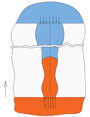
In this work we are primarily concerned with the displacement of one fluid by another immiscible one in capillaries of arbitrary axisymmetric cross-sections. Two cases are investigated; namely, (i) the invading fluid is wetting, and (ii) the invading fluid is non-wetting. In the first case the interface is convex with respect to the invading fluid and is concave for the second one. Because of the continuous change of the radius of the tube along its length, the curvature of the interface also changes. The interfacial tension force, likewise, changes along the tube length. The pressure at the two reservoirs between which the tube terminals are connected are ${p_U}$ at the top reservoir and ${p_D}$ at the bottom reservoir. Figure 1 shows a schematic of the considered set-up with the location of the interface at a distance h(t) from the bottom reservoir and where the length of the tube is H. We are particularly interested in determining the location and velocity of the interface with time. Since the geometric set-up represents a symmetric system, a one-dimensional model along the axis of symmetry employs area average quantities (e.g. the mean velocity). The interfacial tension force along the axis of symmetry not only depends on the contact angle and the radius of the tube, but also on the angle of the tangent to the wall, which changes along the wall of the tube. The radius of the tube along the length is a function of the axial location, or ${r_p} = {r_p}(z)$. In previous studies (e.g. Budaraju et al. Reference Budaraju, Phirani, Kondaraju and Bahga2016), under quasi-static conditions, the radius of curvature $R = R(\vartheta ,z)$ has been assumed to only depend on the contact angle and the radius of the tube, which may not be quite accurate except under very restrictive scenarios $(|\textrm{d}{r_p}/\textrm{d}z|\ll 1)$.

Figure 1. A non-wetting fluid (orange in colour) displaces a wetting one (blue in colour). In this case the pressure of the bottom reservoir must exceed the critical entry pressure for the interface to advance. The radius of the tube changes along its axis i.e. r_p = r_p(z) in a manner that generates a converging, diverging or a combination of them along the tube.

In this work, we slightly relax this restriction and consider the general case in which the radius of curvature of the interface depends, in addition, on the slope of the profile of the tube, that is $R = R(\vartheta ,{r_p},\textrm{d}{r_p}/\textrm{d}z)$. Another restriction with respect to the profile of the capillary tube that is relevant to this study should also be mentioned. It is stipulated that the axial velocity distribution does not significantly deviate from the parabolic profile usually encountered in laminar flows in straight tubes. In order to highlight the variations of the radius of curvature of the interface with the slope of the tube profile and its radius, consider the scenarios shown in figure 2(a,b).

Figure 2. The radius of curvature of the interface depends not only on the contact angle and the radius of the tube but also on the slope of the profile of the tube. Two cases are to be distinguished with respect to whether the interface is at a converging or diverging portion of the tube and also with respect to whether it is an imbibition or drainage scenario. (a) The interface is at a diverging section. (b) The interface is at a converging section.

The interface in this figure represents a non-wetting fluid (orange in colour) displacing a wetting one (blue in colour). At the moment when the interface is located in the diverging portion of the tube (figure 2a) the radius of curvature is $R = {r_p}/\textrm{cos}(\vartheta - \alpha )$ and if the interface is at the converging portion (figure 2b), $R = {r_p}/\textrm{cos}(\vartheta + \alpha )$, where $\alpha = {\tan ^{ - 1}}(\textrm{d}{r_p}/\textrm{d}z)$. As shown in figure 2, the contact angle $\vartheta $ is defined with reference to the invading liquid and the tangent of the profile of the tube. Furthermore, and for the sake of simplicity of the analysis, the dynamic nature of the meniscus is neglected and it is assumed that the contact angle $\vartheta $ remains unchanged throughout the invasion process, which may only be valid under quasi-static conditions.

3. Quasi-one-dimensional modelling approach

The control volume over which the force balance is studied spans the whole length of the capillary tube, as depicted in figure 14. It defines a capillary tube of arbitrary cross-section and a length of H connected from the top and the bottom to two reservoirs.

To simplify the analysis, we consider the upstream and downstream pressures defined right at the entrance and at the exit of the tube. In other words, the predefined pressures at the inlet and the exit of the tube account for the local losses. Although these pressures may change slightly as the pressure field evolves it is expected, over the period of simulation, that predefined volume average pressures may not vary significantly. Compared with the pressure loss along the capillary tube length, the local pressure drop at the entrance is expected to comprise only a small fraction (Budaraju et al. Reference Budaraju, Phirani, Kondaraju and Bahga2016). Furthermore, previous computational fluid dynamics (CFD) investigation shows a slight variation of the axial pressure profiles along the centreline in the reservoir (Salama et al. Reference Salama, Kou, Alyan and Husein2022). More discussion on local entrance losses in such set-ups can be found in several previous works, a good list of which may be found in the work of Waghmare & Mittra (Reference Waghmare and Mittra2010). It is to also be mentioned that the model considers quasi-static analysis in which the contact angle is assumed fixed. The effect of the dynamic behaviour of the contact angle can be captured in a CFD study.

The conservation of linear momentum equation in integral form over a control volume may be written in a vector form as

(3.1)\begin{align}\frac{\partial }{{\partial t}}\int_V {\rho \boldsymbol{u}\,\textrm{d}V} + \int_A {(\rho \boldsymbol{u}\boldsymbol{\cdot }\boldsymbol{n})\boldsymbol{u}\,\textrm{d}A} ={-} \int_A {p\boldsymbol{n}\,\textrm{d}A} + \int_A {\boldsymbol{\tau n}\,\textrm{d}A} + \int_V {\rho \boldsymbol{g}\,\textrm{d}V} + \int_{CL} {\gamma \boldsymbol{t}\,\textrm{d}\ell } ,\end{align}

where $\gamma $ is the interfacial tension, n is the normal to the boundary unit vector, t is the unit vector normal to the contact line (CL) in the plane tangent to the interface, $\boldsymbol{u}$ is the velocity vector of the fluid crossing the boundary, $\boldsymbol{\tau }$ is the viscous stress tensor and p is the pressure. In the above equation, it is assumed that the interface intersects the boundary of the control volume. The left-hand side of the above equation represents inertia of the fluid. As mentioned earlier, the inertial effects are usually limited to the very short time period at the start of the invasion process, (e.g. Salama Reference Salama2021a). It has been estimated elsewhere (e.g. Budaraju et al. Reference Budaraju, Phirani, Kondaraju and Bahga2016; Gorce et al. Reference Gorce, Hewitt and Vella2016) that, for the case in which the two fluids are of comparable density and viscosity, inertial effects may be important for $t \ll \rho {r^2}/\mu $, which is indeed small compared with the time of typical imbibition process. Therefore, it may be possible to ignore the left-hand side of (3.1). For the sake of generality, however, we drive the governing equation including the left-hand side terms. Figure 3 shows a typical capillary tube of arbitrary cross-section along with the two-phase system under both drainage (figure 3a) and imbibition (figure 3b) scenarios. If one applies the conservation of momentum law over the particular control volume shown in figure 3, the right-hand side of (3.1) in the axial direction simplifies to

(3.2)\begin{align} \sum F & = [{p_D}A(0) - {p_U}A(H)] - \int_{{A_1}} {{\tau _1}\,\textrm{d}A} - \int_{{A_2}} {{\tau _2}\,\textrm{d}A} \pm \int_{{V_1}} {{\rho _1}g\,\textrm{d}V}\nonumber \\ & \quad \pm \int_{{V_2}} {{\rho _2}g\,\textrm{d}V} \pm {\rm \pi}D\gamma \,\textrm{cos}[\vartheta + \alpha (h)], \end{align}

where ${p_D}$ and ${p_U}$ are the external pressure at the inlet and exit of the tube, $A(0)$ and $A(H)$ are the cross-sectional areas at the inlet and the exit, respectively, ${\tau _1}$ and ${\tau _2}$ are the shear stresses at the wall of the two portions of the control volume filled with both fluids, ${A_1}$ and ${A_2}$ are the surface areas of the control volume associated with the two fluid regions, ${V_1}$ and ${V_2}$ are the volumes of the respective two fluid regions, ${\rho _1}$ and ${\rho _2}$ are the densities of the fluids in the two parts, $\vartheta $ is the contact angle and $\alpha $ is the angle of the tangent to the tube profile as shown in figure 2. Note that the component of the pressure force in the direction of the flow exerted by the tube wall on the two-phase system is ignored due to the small angle of tangency of the tube profile. Expansion and simplifications of (3.2), yield

(3.3)\begin{align} \sum F & = [{p_D}A(0) - {p_U}A(H)] - 2{\rm \pi} \int_h^H {\tau {r_p}(z)\,\textrm{d}z} - 2{\rm \pi} \int_0^h {\tau {r_p}(z)\,\textrm{d}z}\pm {\rm \pi}{\rho _1}g\nonumber \\ & \quad \int_h^H {r_p^2(z)\,\textrm{d}z} \pm {\rm \pi}{\rho _2}g\int_o^h {r_p^2(z)\,\textrm{d}z} \pm 2{\rm \pi} {r_p}(h)\gamma \,\textrm{cos}[\vartheta - \alpha (h)] = 0. \end{align}

The shear stress at the wall may be written a $\tau (z) ={-} { {\mu \partial u(z)/\partial r} |_{r = {r_p}(z)}}$. Under laminar flow conditions, which may be valid in capillaries, the velocity distribution assumes a parabolic profile and may be represented as $u(r,z) = {U_{max}}[1 - {r^2}/r_p^2(z)]$, where ${U_{max}}$ is the centreline velocity. As indicated earlier, this study considers flows that are approximately uniaxial. Because of the irregular pattern of the tube profile, a cross-flow may be induced. Therefore, this analysis is valid for profiles in which the generated cross-flow is insignificant, which may be achieved when $|{\textrm{d}{r_p}/\textrm{d}z} |\ll 1$. In terms of the average velocity, the above equation may be written as $u(r,z) = 2\bar{U}[1 - {r^2}/r_p^2(z)]$, where $\bar{U}$ is the average velocity. Figure 4 shows a schematic of the parabolic profile.

Figure 3. Schematic of the control volume (dashed line) over which force balance is performed. (a) Drainage and (b) imbibition.

Figure 4. The axial velocity along the radius of the tube may be considered to assume a parabolic profile under laminar flow conditions.

Following Salama (Reference Salama2021a,Reference Salamab), substitution of the shear stress formula into (3.3) and using the volumetric flow rate, $Q = \bar{U}(z)A(z)$, to replace the average velocity, (3.3) reduces to

(3.4)\begin{align} \sum F & = {\rm \pi}[{p_D}r_p^2(0) - {p_U}r_p^2(H)] - 8{\mu _1}Q\int_h^H {\dfrac{{\textrm{d}z}}{{r_p^2(z)}}} - 8{\mu _2}Q\int_0^h {\dfrac{{\textrm{d}z}}{{r_p^2(z)}}}\pm {\rm \pi}{\rho _1}g \nonumber\\ & \quad \int_h^H {r_p^2(z)\,\textrm{d}z} \pm {\rm \pi} {\rho _2}g\int_o^h {r_p^2(z)\,\textrm{d}z} \pm 2{\rm \pi} {r_p}(h)\gamma \,\textrm{cos}[\vartheta - \alpha (h)]. \end{align}

The volumetric flow rate Q in terms of the time derivative of the location of meniscus can be written as $Q = [{\rm \pi} r_p^2(h)]\textrm{d}h/\textrm{d}t$. Substitution into (3.8), simplifications and collecting terms, one obtains

(3.5)\begin{align} \sum F & = {\rm \pi}[{p_D}r_p^2(0) - {p_U}r_p^2(H)] - 8{\rm \pi} {\mu _1}r_p^2(h)\left[ {\int_h^H {\dfrac{{\textrm{d}z}}{{r_p^2(z)}}} + \dfrac{{{\mu_2}}}{{{\mu_1}}}\int_0^h {\dfrac{{\textrm{d}z}}{{r_p^2(z)}}} } \right]\dfrac{{\textrm{d}h}}{{\textrm{d}t}}\nonumber\\ & \quad \pm {\rm \pi}{\rho _1}g\left[ {\int_h^H {r_p^2(z)\,\textrm{d}z} + \dfrac{{{\rho_2}}}{{{\rho_1}}}\int_o^h {r_p^2(z)\,\textrm{d}z} } \right] \pm 2{\rm \pi} {r_p}(h)\gamma \,\textrm{cos}[\vartheta - \alpha (h)]. \end{align}

For simplification of notation, we define the following terms $a(h) = \int_h^H {\textrm{d}z/r_p^2(z)} $, $b(h) = \int_0^h {\textrm{d}z/r_p^2(z)} $, $c(h) = \int_h^H {r_p^2(z)\,\textrm{d}z} $ and $e(h) = \int_o^h {r_p^2(z)\,\textrm{d}z} $.

Substitution into (3.5), one obtains

(3.6)\begin{align} \sum F & = [{p_D}A(0) - {p_U}A(H)] - \left[ {8{\mu_1}{\rm \pi} r_p^2(h)\left( {a + b\dfrac{{{\mu_2}}}{{{\mu_1}}}} \right)} \right]\dfrac{{\textrm{d}h}}{{\textrm{d}t}}\nonumber\\ & \quad \pm {\rm \pi}{\rho _1}g\left[ {c + \dfrac{{{\rho_2}}}{{{\rho_1}}}e} \right] \pm 2{\rm \pi} {r_p}(h)\gamma \,\textrm{cos}(\vartheta - \alpha ). \end{align}

One may define the following two terms, $\lambda = {\mu _2}/{\mu _1}$, and $\xi = {\rho _2}/{\rho _1}$. On substitution into (3.6), one obtains

(3.7)\begin{align} \sum F & = [{p_D}r_p^2(0) - {p_U}r_p^2(H)] - [8{\mu _1}r_p^2(h)(a + b\lambda )]\dfrac{{\textrm{d}h}}{{\textrm{d}t}}\nonumber\\ & \quad \pm {\rho _1}g(c + e\xi ) \pm 2{r_p}(h)\gamma \,\textrm{cos}(\theta - \alpha ). \end{align}

On the other hand, the left-hand side of (3.1) may be written as

(3.8)\begin{align}\textrm{LHS} = \frac{\partial }{{\partial t}}\rho (h)A(h)\frac{{\partial h}}{{\partial t}} + {\rho _1}\left( {\frac{1}{{A(0)}} - \frac{{{\rho_2}/{\rho_1}}}{{A(H)}}} \right){A^2}(h){\left( {\frac{{\partial h}}{{\partial t}}} \right)^2},\end{align}

where $\rho (h) = {\rho _2}h + {\rho _1}(H - h)$, $A(0)$, $A(H)$ and $A(h)$ are the cross-section areas at the inlet, exit and at the location of the meniscus, respectively. The general form of the equation may, therefore, be written as

(3.9)\begin{align} & \dfrac{\textrm{d}}{{\textrm{d}t}}\left[ {\rho (h)A(h)\dfrac{{\textrm{d}h}}{{\textrm{d}t}}} \right] + {\rho _1}\left( {\dfrac{1}{{{A_U}}} - \dfrac{{{\rho_2}/{\rho_1}}}{{{A_D}}}} \right){A^2}(h){\left( {\dfrac{{\textrm{d}h}}{{\textrm{d}t}}} \right)^2}\nonumber\\ & \quad = [{p_D}r_p^2(0) - {p_U}r_p^2(H)] - [8{\mu _1}r_p^2(h)(a + b\lambda )]\dfrac{{\textrm{d}h}}{{\textrm{d}t}} \pm {\rho_1}g(c + e\xi )\nonumber\\ & \quad \quad \pm 2{r_p}(h)\gamma\,\textrm{cos}(\theta - \alpha ). \end{align}

Equation (3.9) is a second-order, nonlinear ordinary differential equation. For the sake of simplicity, if it is possible to ignore the left-hand side terms based on the discussion presented earlier, the above equation reduces to

(3.10)\begin{align} &[{p_D}r_p^2(0) - {p_U}r_p^2(H)] - [8{\mu _1}r_p^2(h)(a + b\lambda )]\frac{{\textrm{d}h}}{{\textrm{d}t}}\nonumber\\ &\quad \pm {\rho _1}g(c + e\xi ) \pm 2{r_p}(h)\gamma \,\textrm{cos}(\theta - \alpha ) = 0.\end{align}

Which for spontaneous imbibition, simplifies to

(3.11)\begin{align}2{r_p}(h)\gamma \,\textrm{cos}(\theta - \alpha ) = {\rho _1}g[c(h) + e(h)\xi ] + \{ 8{\mu _1}r_p^2(h)[a(h) + b(h)\lambda ]\} \frac{{\textrm{d}h}}{{\textrm{d}t}}.\end{align}

Similarly, for upward drainage scenarios, (3.10) may be reformulated as

(3.12)\begin{align}{p_D}r_p^2(0) & = {p_U}r_p^2(H) + {\rho _1}g[c(h) + e(h) \xi ] + 2{r_p}(h)\gamma \,\textrm{cos}[\vartheta + \alpha (h)] \nonumber \\ & \quad + \{8{\mu_1}r_p^2(h)[a(h) + b(h)\lambda] \} \frac{{\textrm{d}h}}{{\textrm{d}t}}.\end{align}

Equation (5.2) represents a model that can handle the invasion process in capillaries of arbitrary shape under the assumption that inertia may be neglected. As seen, (3.10) is a first-order, nonlinear, differential equation for which it may be difficult to find an analytical solution. Furthermore, the integral coefficients a, b, c and e may not always reduce to a closed form. Therefore, a fourth-order Runge–Kutta scheme has been adapted in this study to solve this system.

4. Verification and validation

The case of imbibition and drainage in straight capillaries under the same framework has been considered in Salama (Reference Salama2021a,Reference Salamab). In this section, we show that this developed generalized model reduces to those previously developed models in straight capillary tubes. In this case ${r_p}(z) = \textrm{const}\textrm{.}$, and $\alpha = 0$. The integral coefficients are as follows: $a = (H - h)/r_p^2,\;\; b = h/r_p^2,\; \;c = r_p^2(H - h)$ and $e = r_p^2h$. Substitution yields

(4.1)\begin{align}[{p_D}r_p^2(0) - {p_U}r_p^2(H)] - 8{\mu _1}[H - h + h\lambda ]\frac{{\textrm{d}h}}{{\textrm{d}t}} \pm {\rho _1}gr_p^2[H - h + h\xi ] \pm 2{r_p}\gamma \,\textrm{cos}(\vartheta ) = 0.\end{align}

Collecting terms

(4.2)\begin{align}({p_D} - {p_U}) - \frac{{8{\mu _1}}}{{r_p^2}}[H + h(\lambda - 1)]\frac{{\textrm{d}h}}{{\textrm{d}t}} \pm {\rho _1}g[H + h(\xi - 1)] \pm \frac{{2\gamma \,\textrm{cos}\,\vartheta }}{{{r_p}}} = 0.\end{align}

Factoring

(4.3)\begin{align}\Delta p \pm \frac{{2\gamma \,\textrm{cos}\,\vartheta }}{{{r_p}}} \pm {\rho _1}gH\left[ {1 + \frac{h}{H}(\xi - 1)} \right] - \frac{{8{\mu _1}H}}{{r_p^2}}\left[ {1 + \frac{h}{H}(\lambda - 1)} \right]\frac{{\textrm{d}h}}{{\textrm{d}t}} = 0.\end{align}

Rearrangement

(4.4)\begin{align}\left( {\Delta p \pm \frac{{2\gamma \,\textrm{cos}\,\vartheta }}{{{r_p}}} \pm {\rho_1}gH} \right) \pm {\rho _1}gh(\xi - 1) - \frac{{8{\mu _1}H}}{{r_p^2}}\left[ {1 + \frac{h}{H}(\lambda - 1)} \right]\frac{{\textrm{d}h}}{{\textrm{d}t}} = 0.\end{align}

This last equation is identical to that developed in Salama (Reference Salama2021b), which applies to any combination of two immiscible fluids in capillaries over a large spectrum of density and viscosity contrasts. Furthermore, for spontaneous imbibition in horizontal capillaries between a wetting liquid and air, we have,$\; {\rho _1} \approx 0$, $\; {\mu _1} \approx 0$, $\Delta p = 0$ and $g = 0$, and (4.1) reduces to

(4.5)\begin{align}h\frac{{\textrm{d}h}}{{\textrm{d}t}} = \frac{{\gamma {r_p}\,\textrm{cos}\,\vartheta }}{{4{\mu _2}}}.\end{align}

The solution of the above equation is $h = \sqrt {(\gamma {r_p}t\,\textrm{cos}\,\vartheta )/2\mu } $, which is the celebrated Washburn–Lucas equation. Note that the subscript of ${\mu _2}$ has been dropped for simplicity of notation. Another verification exercise is considered for a case in which the profile of the tube varies. We consider a converging diverging tube as depicted in figure 5(a). The tube profile shows three straight sections connected with two necks representing a converging and a diverging section, (Erickson, Li & Park Reference Erickson, Li and Park2002). Figure 5(b) shows a comparison between the current model and that of Erickson et al. (Reference Erickson, Li and Park2002), who considered the special case of spontaneous imbibition in the system shown in figure 5(a), and as seen, a good match is obtained. The developed model, however, can handle the general case of a two-phase system with arbitrary viscosity and density contrasts with/without gravity.

Figure 5. Schematic of the tube profile (a) as given in Erickson et al. (Reference Erickson, Li and Park2002) that is been used for the comparison and (b) comparison of the location of the meniscus with time. The dimensions are H ₁ = 20 mm, H ₂ = 2.8647 mm, H ₃ = 40 mm, H ₄ = 2.8647 mm, H ₅ = 35 mm, R_max = 50 μm and R_min = 25 μm, and the properties of the imbibing fluid are $\rho = 1000\;\textrm{kg }{\textrm{m}^{ - 3}}$, $\gamma = 0.03\;\textrm{N}\;{\textrm{m}^{ - 1}}$ and $\vartheta = 30^\circ $.

Now, having established the generalized model, it is time to consider some special cases. Three special geometries are considered in the next sections; namely, (i) straight converging/diverging capillaries, (ii) power law capillary profiles and (iii) a sinusoidal profile. In all the considered scenarios, $\textrm{d}{r_p}/\textrm{d}z \ll 1$. Conditions and assumptions of each of the considered scenarios are summarized in table 1 below.

Table 1. Scenarios considered in this work.

5. Quasi-one-dimensional model for capillary flow in a converging/diverging straight tube

Consider the case in which the capillary tube is of a cross-section that changes linearly along the tube length. Two scenarios are possible; namely a converging profile in which the diameter decreases along the length, and a diverging profile when the diameter increases along the length. A generalized linear equation may be written as

(5.1)\begin{align}{r_p}(z) = {r_p}(0) + \frac{{{r_p}(H) - {r_p}(0)}}{H}z.\end{align}

Which in standard form may be written as , where the slope $m = [{r_p}(H) - {r_p}(0)]/H$ can be positive or negative and intercepts , . Figure 6 shows a schematic of one such scenario (the converging profile) in a drainage process. Figure 7, on the other hand, shows the interface as it intersects with the tube wall for both imbibition and drainage scenarios. It is worth mentioning that the angle which the interfacial tension force makes with the axial direction in the drainage scenario is opposite to that in the imbibition scenario, as depicted in figure 7. That is, for example in a converging capillary straight tube, under the drainage scenario, the angle is $(\vartheta + \alpha )$, and for imbibition scenario it is $(\vartheta - \alpha )$. The solution of (3.10) requires the determination of the four parameters a, b, c and e. Luckily, for this scenario, analytical expressions for these parameters may be obtained by evaluating the integrations, as listed in table 1.

Figure 6. Tapered straight capillary tube in the drainage scenario. The orange-coloured region is filled with the non-wetting fluid while the blue-coloured region is the wetting fluid.

Figure 7. Interface in tapered straight tube under imbibition and drainage scenarios. The angle between the direction of the interfacial tension force and the axial direction (z-direction) is given by $\; \vartheta \pm \alpha $, where $\alpha $ is the angle between the tangent to the tube profile and the z-direction. (a) Drainage (converging profile), (b) drainage (diverging profile), (c) imbibition (converging profile) and (d) imbibition (diverging profile).

It is interesting to highlight some key features of this system by comparing the speed of the meniscus at the beginning (i.e. when it is at the entrance) and at the exit of the tube. For simplicity, we consider a spontaneous imbibition scenario in horizontal capillaries. In this case (4.4) reduces to

(5.2)\begin{align}\frac{{\textrm{d}h}}{{\textrm{d}t}} = \frac{{2\gamma \,\textrm{cos}(\theta + \alpha )/{r_p}(h)}}{{\{ 8{\mu _1}[a(h) + b(h)\lambda ]\} }}.\end{align}

Table 1 Analytical expressions for the parameters a, b, c and e for the cases of imbibition and drainage in converging/diverging straight capillaries.

(5.3 & 5.4)

(5.5, 5.6 & 5.7)

Substitution of the parameters $a(h)$ and $b(h)$ as given in (5.3) and (5.4), yields

(5.8)

With simplifications and rearrangements, one finds

(5.9)

Therefore, at the beginning of the imbibition process (i.e. h = 0), (5.9) simplifies to

(5.10)\begin{align}u(0) = {\left. {\frac{{\textrm{d}h}}{{\textrm{d}t}}} \right|_{h = 0}} = \frac{{\gamma \,\textrm{cos}(\theta + \alpha ){r_p}(H)}}{{4{\mu _1}H}}.\end{align}

Furthermore, when h = H one obtains

(5.11)\begin{align}{\left. {u(H) = \frac{{\textrm{d}h}}{{\textrm{d}t}}} \right|_{h = H}} = \frac{{\gamma \,\textrm{cos}(\theta + \alpha ){r_p}(0)}}{{4{\mu _1}\lambda H}}.\end{align}

Now, the ratio between the velocities of the meniscus at the exit and at the inlet is

(5.12)\begin{align}\frac{{u(H)}}{{u(0)}} = \frac{{{r_p}(0)/{r_p}(H)}}{\lambda }.\end{align}

For the special case in which ${r_p}(0)/{r_p}(H) = \lambda $, the velocity ratio is one, which implies that the meniscus moves at a constant speed. Furthermore, if ${r_p}(0)/{r_p}(H) > \lambda $, the speed of the meniscus increases and decreases otherwise. It is interesting to notice that, $\textrm{if}\;\; {r_p}(0) = {r_p}(H)$, which corresponds to the case of a straight uniform tube, the velocity ratio is $1/\lambda $. For the case of a diverging tube in which ${r_p}(0)/{r_p}(H) < 1$, $u(H)$ is always smaller than $u(0)$. One can also investigate the ratio of the velocities of the meniscus at the exit of the tube for different converging or diverging scenarios for the same fluids. For two profiles of different angles $\alpha $ but the same${r_p}(0)$, the ratio of the velocities is ${u_1}(H)/{u_2}(H) = \textrm{cos}(\theta + {\alpha _1})/\textrm{cos}(\theta + {\alpha _2})$. For longer tubes, $\alpha $ is usually small, which leads to${u_1}(H) \approx {u_2}(H)$. This is interesting and is a manifestation of the fact that when the meniscus reaches the exit, the tube becomes filled with only the invading fluid. In this case the friction force will only depend on the size of the tube, and both the friction and the capillary forces are oppositely correlated with the size of the pore. Therefore, for the smaller size pore opening at the exit, the capillary force increases and likewise the friction force and this seems to cancel out their effect. Likewise, for the same ${r_p}(0)$, the ratio between the velocities of the meniscus at the beginning of its movement is

(5.13)\begin{align}\frac{{{u_1}(0)}}{{{u_2}(0)}} = \frac{{\textrm{cos}(\theta + {\alpha _1}){{[{r_p}(H)]}_1}}}{{\textrm{cos}(\theta + {\alpha _2}){{[{r_p}(H)]}_2}}}.\end{align}

Which, again for longer tubes, simplifies to ${u_1}(0)/{u_2}(0) \approx {[{r_p}(H)]_1}/{[{r_p}(H)]_2}$. This may be read as follows: for the same fluids and ${r_p}(0)$, the inlet velocity is larger the larger the size of the opening at the exit. This conclusion, in fact, should come as no surprise on account of the fact that the larger size pore opening implies less overall resistance, hence the above observation. An analytical expression can be derived that depicts the dynamics of the meniscus along the tube length. A derivation can be found in Appendix A. It takes the form

(5.14)\begin{align}\frac{{(\lambda - \beta )}}{{2H\psi }}{h^2} + \frac{\beta }{\psi }h = t,\end{align}

where $\beta = {r_p}(0)/{r_p}(H)$, and $\psi = \gamma {r_p}(0)\,\textrm{cos}(\theta + \alpha )/4{\mu _1}H$. These conclusions are manifested on applying the developed model on the two cases of imbibition in converging and diverging straight capillaries. In all the considered scenarios, the viscosity ratio between the invading fluid and the displaced one is set to 100, the surface tension to 0.072 N m⁻¹ and the contact angle is 45°. Starting with the case of imbibition in converging straight pipes in which the radius of the tube at the inlet, $\; {r_p}(0)$, for all the scenarios is set to 0.0005 m. At the exit, the tube assumes radii of $5 \times {10^{ - 4}}$, $5 \times {10^{ - 5}}$, $2.5 \times {10^{ - 5}}$, $1.25 \times {10^{ - 5}}$, $5 \times {10^{ - 6}}$ and $1.25 \times {10^{ - 6}}$ m. This corresponds to radius ratios, i.e. $\; {r_p}(H)/{r_p}(0)$, of 1.0, 0.1, 0.05, 0.025, 0.01 and 0.0025, respectively, with the case in which the radius ratio is 1 representing a straight tube. Figure 8 shows the location of the meniscus along the tube with time for the different scenarios. It is more appropriate to scale the time by$\; T = 2\mu {H^2}/\gamma {r_p}(0)\,\textrm{cos}\,\vartheta $, which represents the total time at which the meniscus would reach the exit of the straight tube. As has been stated earlier, the scenario in which the radius ratio equals the viscosity ratio defines the boundary between the two cases. In the first case, in which $\; {r_p}(H)/{r_p}(0) > 1/\lambda $, after the initial period, the velocity of the meniscus decelerates with time. This implies that the friction force dominates the capillary force in these cases. In the second case, i.e. when ${r_p}(H)/{r_p}(0) < 1/\lambda $, the opposite occurs and the meniscus accelerates, which indicates that the capillary forces dominate the viscous force. When ${r_p}(H)/{r_p}(0) = 1/\lambda $, the meniscus moves at a constant speed. These conclusions, which have been deduced from analysing the model, are confirmed as depicted in figure 8.

Figure 8. The normalized location of the meniscus along the tube for the different converging scenarios. When the radius ratio equals the viscosity ratio, the speed of the meniscus is constant and, in this case, the capillary force and viscous force balance each other $({h^\ast } = h/H,\;{t^\ast } = t/T)$.

Furthermore, the exit speed of the meniscus is approximately the same for the different scenarios, which is also seen in figure 8. That is, the slopes at the end of these curves (which represents the velocity) are indeed approximately the same. This is also manifested in figure 9, which shows the profiles of the speed of the meniscus with time for the different scenarios. At the exit, the speed of the meniscus, for all the scenarios, converges to almost the same speed. This has been highlighted in the earlier discussion and indicates the fact that the interplay between viscous and capillary forces is such that they both increase along the tube length. At the start of the imbibition process, the initial velocity is dictated by the initial overall resistance of the tube, which is larger the narrower the tube at the exit. In other words, when the meniscus is at the inlet of the tube, for all the scenarios, the capillary force, which is approximately identical at the start, is opposed by larger viscous resistance when the size of the pore at the exit is smaller. This leads the meniscus to acquire a larger initial speed when the size of the tube at the exit is larger and vice versa. This behaviour is manifested in figure 9, which shows the velocity profiles of the meniscus for the different scenarios.

Figure 9. Velocity profiles for the case of a converging straight tube. The ratio of the radius of the tube between the exit and the inlet, i.e. $\; {r_p}(H)/{r_p}(0)$, changes between 1 (for straight tube) and 0.0025. The speed of the meniscus drops initially at a faster pace then at a lower rate towards the end until the meniscus reaches the exit. (Note the time is normalized by $T = 2\mu {H^2}/\gamma {r_p}(0)\,\textrm{cos}\,\vartheta $.)

When the meniscus is at the exit, on the other hand, the larger overall viscous resistance when the exit of the tube is smaller is counteracted by a larger capillary force. In other words, the capillary force at the exit of the tube is not the same for all the scenarios and this explains the noticed behaviour.

The case of a diverging straight tube is also considered in this work. The radius of the tube at the inlet for all the scenarios has been set to 0.00005 m and at the exit, it follows radius ratios, ${r_p}(H)/{r_p}(0)$, of 1, 5, 10, 25 and 50. Unlike the converging scenario, the location of the meniscus for all the scenarios of a diverging tube follows a relatively similar profile as depicted in figure 10. The fact that there is no significant difference in the profiles that depict the location of meniscus in all the scenarios is interesting and is a reflection of the interplay between viscous and capillary forces, with both decreasing along the tube length. When the meniscus is at the inlet of the tube, the capillary force for all the scenarios is approximately similar. However, the overall friction force is different for the different scenarios with it being larger the smaller the size of the tube at the exit.

Figure 10. Profiles of the location of the meniscus with time (normalized by$\; T = 2\mu {H^2}/\gamma {r_p}(0)\,\textrm{cos}\,\vartheta $) for the different diverging profile cases. The radius at the exit of the tube changes between 1 (for straight tube) and 50 times of that at the inlet. As seen, the profiles look similar for all the cases.

Therefore, we would expect there are variations of the speed of the menisci at the inlet, which is indeed depicted in figure 11. At the exit, the story is opposite to that of the converging tube scenario. That is, the capillary force at the exit becomes smaller compared with its value at the inlet. The lowest capillary force would occur when the meniscus reaches the exit of the tube (i.e. at the larger cross-section) and likewise the friction force. This simply leads the speed of the meniscus at the exit to be almost the same, which conforms to the discussion outlined earlier. A more detailed discussion about the effects of the different geometrical factors (i.e. the parameters a, b, r_p(h)) on both the friction and capillary forces is given in Appendix B. It highlights how the friction and capillary forces change along the tube length, and how this explains the different behaviour of the meniscus along the tube.

Figure 11. Velocity profiles for the diverging scenarios on a logarithmic scale. The velocities at the start are different and they converge at the end.

6. Quasi-one-dimensional model for power-law-shaped converging/diverging capillaries

This is another interesting case in which the tube assumes a nonlinear profile. Both converging and diverging profiles are considered. The interesting thing in this case is the fact that the angle of tangency along the tube length (i.e. α) changes continuously and should be incorporated as a variable rather than just a constant. Moreover, the influence of the angle of tangency is expected to show an influence on the profiles of the speed of the meniscus. In this scenario, the profile of the tube takes the general form as given below

(6.1)\begin{align}{r_p}(z) = {r_p}(0)\epsilon {z^n},\quad n > 1,\end{align}

where $\epsilon $ is a parameter with its sign defines whether the profile is converging (i.e. when $\epsilon < 0$) or diverging (i.e. when $\epsilon > 0$). If ${r_p}(H)$ is known a priori, then $\epsilon = [{r_p}(H) - {r_p}(0)]/{H^n}$.

We define $r_p^\ast{=} {r_p}(z)/{r_p}(0)$, $\; {z^\ast } = z/H$ and $\omega = \epsilon {H^n}/{r_p}(0)$, (6.1) may, therefore, be written in a dimensionless form as

(6.2)\begin{align}r_p^\ast{=} 1 + \omega (n){z^{{\ast} n}}.\end{align}

Figure 12(a) shows a diverging profile for the case when $n = 2$, and $\omega = 1.0$. Similarly, figure 12(b) shows a converging one when $n = 2$, and $\omega ={-} 0.5$. For the sake of illustration, we consider imbibition scenarios over quadratic profiles (i.e. the exponent n is 2). For this profile, the analytical expressions for the parameters a, b are long and complex, however, they are relatively simple for the other two parameters c, and e, which are expressed as

(6.3)\begin{gather}c(h) = \frac{{3{H^5}{\epsilon ^2} + 10{H^3}{r_p}(0)\epsilon + 15Hr_p^2(0)}}{{15}} - \frac{{3{h^5}{\epsilon ^2} + 10{h^3}{r_p}(0)\epsilon + 15hr_p^2(0)}}{{15}},\end{gather}

(6.4)\begin{gather}e(h) = \frac{{3{h^5}{\epsilon ^2} + 10{h^3}{r_p}(0)\epsilon + 15hr_p^2(0)}}{{15}}.\end{gather}

Figure 12. Two normalized quadratic profiles as an example of a power law capillary tube. (a) A diverging profile and (b) a converging profile.

Furthermore, the slope of the tube profile changes along the tube length. The slope will be negative for the converging profile and positive otherwise. It may be given as

(6.5)\begin{align}\alpha (h) = \frac{{\textrm{d}{r_p}}}{{\textrm{d}z}} = 2\epsilon h.\end{align}

We first investigate the case of a converging quadratic profile. In this case, the radius of the tube at the inlet is considered as 0.005 m and at the exit it takes a value corresponding to the radius ratios of 1.0, 0.1, 0.05, 0.01 and 0.005, respectively. Figure 13 shows the profiles of the location of the meniscus with time for the different scenarios. Apart from the straight tube profile, which shows that the profile steadily progresses with a decreasing slope, for the case of a quadratic converging profile the slope changes in a different manner, as depicted in figure 13. The slope of the profile of the location of the meniscus decreases at early times, implying a decrease in the velocity of the meniscus, it then increases again, implying an increase in the velocity of the meniscus. This can be explained in light of the relationship between capillary and friction forces. During the early time, the friction force dominates and this leads to a decrease in the velocity of the meniscus. Later on, the capillary force takes over and this results in an increase in the velocity of the meniscus. More insight into this can be found in Appendix B in the context of converging straight tubes. Furthermore, the profiles show that the meniscus takes longer to reach the end of the tube when the radius ratio is smaller, which is a manifestation of the increased friction.

Figure 13. Profiles of the location of the meniscus along the tube for different radius ratios for quadratic converging tube profiles.

Figure 14. Velocity profile of the meniscus with time for the quadratic converging tube profile. Three time periods can be identified, namely, (i) a period at the start where the speed drops, (ii) a period in the middle where the speed plateaus and (iii) a period at the end where the speed increases.

This behaviour is also depicted in figure 14, which shows the profile of the speed of the meniscus for the different scenarios. It is clear that the speed of the meniscus drops at the start at a faster pace, plateaus, then increases again. This is interesting and implies, as mentioned before, that at the beginning the friction force grows quickly (faster than the capillary force), reducing thereby the speed of the meniscus. The two forces then approximately balance each other and the speed of the meniscus plateaus. Towards the end, the capillary force takes over and the speed of the meniscus increases. To highlight the initial speed of the meniscus for the different scenarios at the start of the imbibition process, figure 15 is a reproduction of figure 14 on a logarithmic scale. It shows the speeds of the meniscus at the start of the imbibition process (they are different) and likewise at the end (they are approximately the same).

Figure 15. Velocity profile of the meniscus over a logarithmic scale for the converging, quadratic tube profile.

For the case of a diverging quadratic profile, the radius of the tube at the entrance for all the scenarios is considered as 0.00005 m. At the exit, the radius of the diverging tube varies according to radius ratios of 1, 5, 10, 25 and 50. Figure 16 shows the profiles of the location of the meniscus along the tube and, as depicted, the time spans until the meniscus reaches the end of the tube are different (being longer when the tube radius at the exit is larger). This is unlike the case when the diverging tube follows a linear pattern, which shows relatively similar profiles as shown in figure 10. This may be explained in light of the behaviour of the friction and capillary forces along the tube. It is evident that the friction force increases with the nonlinear increase in the tube diameter along its length more than the increase in capillary force. This results in the speed of the meniscus decreases as the diameter ratio increases and explains the longer time it takes for the meniscus to reach the end of the tube as the diameter ratio increases. More insight can be inferred from the discussion presented in Appendix B.

Figure 16. The profile of the location of the meniscus (normalized by the length of the tube) with time normalized by the total time the meniscus needs to reach the exit of a straight tube (i.e. $T = 2\mu {H^2}/\gamma {r_p}(0)\,\textrm{cos}\,\vartheta $).

Velocity profiles, likewise, drop at a faster rate at the start and then at a slower rate, as depicted in figure 17. To capture the variations of the velocity of the meniscus at the start and at the end, figure 17 is reproduced over a logarithmic scale, which is illustrated in figure 18.

Figure 17. Velocity profile for a diverging quadratic tube profile on a linear scale.

Figure 18. Velocity profile for a diverging quadratic tube profile on a logarithmic scale.

As depicted, the initial velocity is larger the larger the diameter ratio. At the end, however, it is interesting to note that, unlike the case of a diverging straight tube where the velocity at the exit is similar for all the scenarios, this is not the case when the tube profile is nonlinear. This may be explained as previously mentioned in relation to the ratio ${u_1}(H)/{u_2}(H) = \textrm{cos}(\theta + {\alpha _1})/\textrm{cos}(\theta + {\alpha _2})$. When the tube is nonlinearly diverging, the angles ${\alpha _1}$, and ${\alpha _2}$ may not be ignored and this explains the noticed behaviour.

7. Quasi-one-dimensional model for sinusoidal-shaped capillaries

This is an interesting scenario because it involves both converging and diverging parts in one profile. A general sinusoidal profile takes the form

(7.1)\begin{align}{r_p} = \frac{{{r_{p,max}} - {r_{p,min}}}}{2}\,\textrm{sin}\left( {2{\rm \pi} \frac{z}{\varepsilon }} \right) + \frac{{{r_{p,max}} + {r_{p,min}}}}{2},\end{align}

where $\varepsilon $ is the wavelength and is chosen such that $\varepsilon /H\sim {O}(1)$, as depicted in figure 19. Let $A = ({r_{p,max}} - {r_{p,min}})/2$, and $B = ({r_{p,max}} + {r_{p,min}})/2$, then the above equation simplifies to

(7.2)\begin{align}{r_p} = A\,\textrm{sin}(Bz) + C.\end{align}

Figure 19. Schematic of a capillary tube with sinusoidal profile.

In accordance with lubrication theory (Budaraju et al. Reference Budaraju, Phirani, Kondaraju and Bahga2016), it may be required that $A \ll 1$, which may also be translated as $\textrm{d}{r_p}/\textrm{d}z \ll 1$. This implies that the transverse length scale of the flow is small compared with the length scale in the flow direction, which is indeed the case in capillaries. Again, the coefficients a and b are quite complex and lengthy, however, the coefficients c and e may be found by evaluating the integrations. They take the forms

(7.3)\begin{gather}\begin{array}{ccccc} c & = \dfrac{{{A^2}\,\textrm{sin}(2Bh) + 8AC\,\textrm{cos}(Bh) - (4B{C^2} + 2{A^2}B)h}}{{4B}}\\ & \quad - \dfrac{{{A^2}\,\textrm{sin}(2BH) + 8AC\,\textrm{cos}(BH) - (4B{C^2} + 2{A^2}B)H}}{{4B}}, \end{array}\end{gather}

(7.4)\begin{gather}e = \frac{{2AC}}{B} - \frac{{{A^2}\,\textrm{sin}(2Bh) + 8AC\,\textrm{cos}(Bh) - (4B{C^2} + 2{A^2}B)h}}{{4B}}.\end{gather}

The interesting thing about this scenario stems from the fact that it mimics, to some extent, a tortious path, which fluids usually encounter in porous medium flows. Therefore, it would be interesting to explore this scenario in order to investigate how the meniscus will behave in such cases. In all the considered scenarios, the following parameters are set constant

The parameter that is set free is the wavenumber, $\kappa = H/\varepsilon $, which determines the number of full cycles along the tube length. In this work, the values of $\kappa $ that are considered include 0, 3, 4 and 5, with the value of 0 representing the case of a straight tube. The angle of tangency (α) of the tube profile is $\alpha = \textrm{ta}{\textrm{n}^{ - 1}}(\textrm{d}{r_p}/\textrm{d}z)$, with $\textrm{d}{r_p}/\textrm{d}z = AB\,\textrm{cos}(Bz)$.

The normalized location of the meniscus is plotted against normalized time for the different scenarios and is shown in figure 20 for different wavenumbers. In addition, two cases of straight tubes with radii equal to ${r_{p,min}}$ and ${r_{p,max}}$, are also considered. It is clear that the profiles of the location of the meniscus of all the considered scenarios are set between the two straight cases. Furthermore, they feature a wavy nature as a consequence of the sinusoidal profile of the tube with number of cycles in accordance with that of the tube.

Figure 20. The normalized location of the meniscus with normalized times for different wavenumbers. In addition, two scenarios of straight tubes with the same maximum and minimum radii are also shown.

Such a wavy nature of the location of the meniscus implies a similar wavy pattern for the speed of the meniscus as depicted in figure 21 (on a linear scale) and figure 22 (on logarithmic scale). From figure 21, it is clear that the speed of the meniscus generally decreases along the tube length. Furthermore, the period of change of the speed along the tube also changes with time (being longer at later time), which is a manifestation of the decrease in the average speed with time.

Figure 21. Velocity profile for the case of a sinusoidal tube profile with different cycles along the length of the tube on a linear scale.

Figure 22. Velocity profiles for different wavenumbers in cycles/m over a logarithmic scale.

8. Imbibition against gravity

When gravity is involved, which corresponds to the case of a vertically, upward-oriented capillary tube, if the tube is long, an interesting possibility arises. This is when the capillary force is balanced by the gravitational force and the interface ceases to climb upwards at a particular height, called the equilibrium height. While it is relatively simple to estimate this height in straight capillaries, it is not that straightforward when the radius of the tube changes along its length. In this case, the radius of curvature of the interface is a function of the profile of the tube, i.e. ${r_p} = {r_p}(h)$. When gravity is present, a nonlinear equation may be developed for the equilibrium height, the roots of which determine such a height. The equation that governs imbibition in which gravity exists may be written as

(8.1)\begin{align}- [8{\mu _1}r_p^2(h)(a + b\lambda )]\frac{{\textrm{d}h}}{{\textrm{d}t}} - {\rho _1}g(c + e\xi ) + 2{r_p}(h)\gamma \,\textrm{cos}(\theta - \alpha ) = 0.\end{align}

When the meniscus has reached its terminal location, it is obvious that its speed becomes zero, or $\textrm{d}h/\textrm{d}t = 0$. Substitution into the above equation yields

(8.2)\begin{align}{\rho _1}g[c(h) + \xi e(h)] = 2{r_p}(h)\gamma \,\textrm{cos}[\theta - \alpha (h)].\end{align}

On rearrangement, one obtains

(8.3)\begin{align}{r_p}(h) = \frac{{{\rho _1}g[c(h) + \xi e(h)]}}{{2\gamma \,\textrm{cos}[\theta + \alpha (h)]}}.\end{align}

The integral parameters c and e are geometrical factors that depend on the profile of the tube and are, therefore, functions of h. For the case of a linearly varying converging/diverging capillary tube, we have ${r_p}(h) = {r_p}(0) + mh$. Substitution yields the following relationship for the equilibrium height:

(8.4)\begin{align}h = \frac{{{\rho _1}g(c + e\xi )}}{{2\gamma m\,\textrm{cos}(\theta + \alpha )}} - \frac{{{r_p}(0)}}{m}.\end{align}

Let $\varLambda = {\rho _1}g/2\gamma \,\textrm{cos}(\theta + \alpha )$, then the above equation reduces to

(8.5)\begin{align}mh = \varLambda (c + e\xi ) - {r_p}(0).\end{align}

On rearrangement, we get the following nonlinear equation for the terminal height in the form $f(h) = \textrm{const}\textrm{.}$, or:

(8.6)\begin{align}f(h) = \varLambda \textrm{[}c(h) + \xi e(h)] - mh = {r_p}(0).\end{align}

The parameters $c(h)$, and $e(h)$ are as given in table 1. The admissible root of the above equation determines the terminal location of the meniscus. One may observe that, for a diverging straight tube (i.e. $m > 0$), the larger the value of m, the smaller h will be. Conversely, for a converging tube (i.e. $m < 0$), the larger the value of m, the larger h will be. For the sake of illustration, let us consider the following examples of a converging and a diverging linear straight tube scenario. The first case represents a diverging capillary tube with ${r_p}(H)/{r_p}(0) = 10$. Parameters used for the example of a capillary rise in a diverging tube with a diameter ratio of 10 are listed below.

Implementing these parameters into (8.6), one may be able to find the value of the equilibrium height, h. A graphical implementation of the above equation is shown in figure 23. The function in (8.6) is modified by dividing through by m. It takes the form $f(h) = (\varLambda /m)[c(h) + \xi e(h)] - h$, and the right-hand side is ${r_p}(0)/m$. For a diverging scenario, the parameters used are those listed above. For the converging scenario, the parameters are the same except that the radius ratio ${r_p}(H)/{r_p}(0)$ is 0.1, with both having the same ${r_p}(0)$. The intersection of $f(h)$ and the constant ${r_p}(0)/m$ define the location of the meniscus at equilibrium. Furthermore, the two cases were also investigated using the developed model and were solved numerically, as given previously, and an almost exact match is obtained. Figure 24(a) shows the profiles depicting the location and the speed of the meniscus with time for the diverging scenario. As is clear, the location of the meniscus asymptotically approaches an equilibrium height of 0.075 m. This conforms to that theoretically derived, as depicted in figure 23(b). For a converging capillary, on the other hand, the location of the meniscus is found to be approximately 0.103 m, as obtained using both the developed general model and the analytical one (figure 23c,d).

Figure 23. Equilibrium height for converging/diverging straight tubes, h* is the normalized location of the meniscus and u is its speed. The intersection of the function f(h), $[f(h) = (\varLambda /m)[c(h) + \xi e(h)] - h]$ and the line ${r_p}(0)/m$ defines the solution of (8.6), which determines the location of the meniscus. (a) Simulated equilibrium height (diverging straight tube). (b) Calculated equilibrium height (diverging straight tube). (c) Simulated equilibrium height (converging straight tube). (d) Calculated equilibrium height (diverging straight tube).

Figure 24. Imbibition in converging/diverging quadratic tube profiles (a,b) as well as in sinusoidal one (c) when gravity is considered. The profiles approach asymptotically the equilibrium height. (a) Converging quadratic tube: $H = 1.0\; \;\textrm{m}$, ${r_p}(0) = 1.0 \times {10^{ - 4}}\;\textrm{m}$, ${r_p}(H) = 1.0 \times {10^{ - 5}}\;\textrm{m}$, ${r_p}(H)/{r_p}(0) = 0.1$, $\epsilon = [{r_p}(H) - {r_p}(0)]/{H^2} ={-} 0.00009$, ${r_p}(z) = 0.0001 - 0.00009{z^2}$. (b) Diverging quadratic tube: ${H = 1.0\;\textrm{m}}$, ${r_p}(0) = 1.0 \times {10^{ - 4}}\;\textrm{m}$, ${r_p}(H) = 1.0 \times {10^{ - 3}}\;\textrm{m}$, ${r_p}(H)/{r_p}(0) = 10$, $\epsilon = [{r_p}(H) - {r_p}(0)]/{H^2} = 0.0009$, ${r_p}(z) = 0.001 + 0.0009{z^2}$. (c) Sinusoidal profile: $H = 1.0\;\textrm{m}$, ${r_{p,min}} = 1.0 \times {10^{ - 4}}\;\textrm{m}$, ${r_{p,max}} = 1.0 \times {10^{ - 3}}\;\textrm{m}$, ${r_{p,max}}/{r_{p,min}} = 10$, $n = \# \; Cycles = 5$.

For the sake of comparison, it is interesting to examine the location of the meniscus at equilibrium for a straight tube with the same ${r_p}(0)$. Using the formula $h = 2\gamma \,\textrm{cos}\,\vartheta /{r_{p0}}\rho g$, one finds that h = 0.104 m, which is larger than those for converging and diverging scenarios.

To enlarge the scope of the comparisons with respect to the ratio between the equilibrium height of a straight capillary tube with that of converging/diverging ones of arbitrary radius ratio, an analysis of this topic is highlighted in this section. For simplicity, let us focus our attention to the case of spontaneous imbibition, where the displaced fluid is a gas. It is known that, at equilibrium, both the gravity and capillary forces balance each other. Analysis in Appendix C shows that

(8.7)\begin{align}\frac{{{h_{C/D}}}}{{{h_S}}} = \frac{{3\,\textrm{cos}(\vartheta + \alpha )/\textrm{cos}\,\vartheta }}{{\left[ {\frac{{{r_{p0}}}}{{{r_{ph}}}} + \frac{{{r_{ph}}}}{{{r_{p0}}}} + 1} \right]}},\end{align}

where ${h_{C/D}}$ is the equilibrium height of the meniscus in a converging/diverging capillary tube, ${h_S}$ is the equilibrium height of the meniscus inside a straight tube with the same radius at the inlet, ${r_{p0}}$ is the tube radius at the inlet, ${r_{ph}}$ is the tube radius at the location of the meniscus and $\alpha $ is the angle of inclination of the converging/diverging tube. Derivation of the above equation is presented in Appendix C. For the case in which $\alpha $ is small, the above equation reduces to

(8.8)\begin{align}\frac{{{h_{C/D}}}}{{{h_S}}} = \frac{3}{{\left[ {\frac{{{r_{p0}}}}{{{r_{ph}}}} + \frac{{{r_{ph}}}}{{{r_{p0}}}} + 1} \right]}}\; .\end{align}

Furthermore, when ${r_{p0}} = {r_{ph}}$ (i.e. straight tube), the above ratio is one. Equation (8.8) indicates that the equilibrium height for a converging/diverging straight tapered tube is always smaller than that of the corresponding straight tube with the same inlet radius. It is interesting to also explore the cases of converging/diverging and sinusoidal profiles for the cases of upward imbibition against gravity. Figure 24 shows the profiles of the location of the meniscus for the case of a converging/diverging quadratic and sinusoidal profiles, with the geometric parameters as given on the figures.

As one notices, the gravity equilibrates the interfacial force within the tube. This is manifested by noticing the profiles of the location of the meniscus, which show that they reach a terminal location inside the tubes. For the case of a converging quadratic tube with parameters as given in figure 24(a), the meniscus rises to a height of approximately 0.103 m, which is slightly smaller than that of a straight tube of the same ${r_p}(0)$. For the case of a diverging quadratic profile with parameters as given in figure 24(b), the meniscus equilibrates at a height of 0.0835 m. Lastly, for the case of sinusoidal profile (figure 24c), the meniscus equilibrates at a height of 0.017 m. In other words, the equilibrium height for all the considered profiles is smaller than that of a straight tube having the same inlet radius. Finally, the model, as developed, can be implemented in studying two-phase flows in porous media (El Amin, Salama & Sun Reference El Amin, Salama, Sun and El-Amin2011) as well as in dynamic pore network models to locate the meniscus as it develops in the pore throats. It can also be used in the modelling of the filtration of emulsions using polymeric-type membranes (Salama, Zoubeik & Henni Reference Salama, Zoubeik and Henni2017; Zoubeik, Salama & Henni Reference Zoubeik, Salama and Henni2018; Echakouri, Salama & Henni Reference Echakouri, Salama and Henni2020)