


1. Introduction
Since the seminal work of Mollo-Christensen (Reference Mollo-Christensen1967), coherent structures and their role in sound generation have been one of the main focuses of studies in the jet aeroacoustics community. As summarised by Jordan & Colonius (Reference Jordan and Colonius2013), jets are subject to a hydrodynamic instability mechanism (the Kelvin–Helmholtz (KH) mode) that generates a large-scale, spatially coherent structure characterised by oscillatory behaviour, with an exponential growth in early stages of the jet, followed by saturation and decay further downstream – thus receiving the name ‘wavepackets’. These structures are a key part of the sound generation mechanism for both subsonic (Crighton Reference Crighton1975; Cavalieri et al. Reference Cavalieri, Jordan, Colonius and Gervais2012; Baqui et al. Reference Baqui, Agarwal, Cavalieri and Sinayoko2015; Cavalieri, Jordan & Lesshafft Reference Cavalieri, Jordan and Lesshafft2019) and supersonic (Tam Reference Tam1995; Nichols & Lele Reference Nichols and Lele2011; Sinha et al. Reference Sinha, Rodríguez, Brès and Colonius2014) jets.
When dealing with imperfectly expanded supersonic jets, the presence of a coherent shock-cell structure (Pack Reference Pack1950) markedly changes the overall characteristics of the acoustic field. Three noise components can now be identified in the flow (Tam Reference Tam1995). The first, common to subsonic and supersonic jets, is the turbulent mixing noise, which is directly associated with the large-scale structures; for supersonic jets, this component is highly directional (focused on downstream angles) and generally peaks at lower frequencies of the acoustic spectrum. The second component is related to the interaction between the large-scale structures and the shock-cell structure – the broadband shock-associated noise (Harper-Bourne & Fisher Reference Harper-Bourne and Fisher1974). This component has significant amplitudes for higher frequencies and in contrast to turbulent mixing noise, the maximum intensity of this component peaks in the perpendicular/upstream directions. The third component, usually of higher intensity, is the screech tone. Screech is characterised by a sharp peak in the acoustic spectrum, and is associated with high-amplitude oscillations of the jet, being a consequence of a resonance phenomenon.
Screech was first studied by Powell (Reference Powell1953a), who characterised the phenomenon using schlieren photographs. Powell identified the presence of two types of waves in the flow travelling in opposite directions: large-scale downstream-travelling waves, which were later identified as the KH mode, and upstream-travelling waves, which were considered to be free-field acoustic waves. From his early works, four processes of the resonance loop can be educed (Edgington-Mitchell Reference Edgington-Mitchell2019): (i) the downstream propagation of energy, which is due to the large-scale downstream-travelling waves in these jets; (ii) an energy reflection mechanism, in which downstream-travelling disturbances generate upstream-travelling waves; (iii) the upstream propagation of disturbances; and (iv) the forcing of new downstream-travelling waves by the upstream waves in a sensitive point of the flow. Several works built upon the results of Powell (Reference Powell1953a), identifying a number of characteristics of screeching jets. Merle (Reference Merle1956) followed by Davies & Oldfield (Reference Davies and Oldfield1962) identified oscillation regimes of imperfectly expanded jets, highlighting the different characteristics of the hydrodynamic waves present in each mode. They also showed that different regimes are observed as the nozzle pressure ratio (NPR) is increased, and these have a strong effect on the screech frequency and the dynamics of the jet, leading to changes in the dominant azimuthal wavenumber of the disturbances. The phase and gain conditions for self-sustaining resonant cycles proposed by Powell (Reference Powell1953b) were also used to build resonance models for predicting screech frequencies in the different jet regimes; most of these are summarised in the reviews by Raman (Reference Raman1998) and Edgington-Mitchell (Reference Edgington-Mitchell2019).
The development of linear stability analysis (LSA) allowed for a better characterisation of the different waves involved in the phenomenon. The association of the large-scale, downstream-travelling structure with the KH instability mode comes directly from works such as Michalke (Reference Michalke1970), Crow & Champagne (Reference Crow and Champagne1971), Cavalieri et al. (Reference Cavalieri, Rodríguez, Jordan, Colonius and Gervais2013) and Sinha et al. (Reference Sinha, Rodríguez, Brès and Colonius2014), who managed to identify some of the characteristics of this structure using linear models. Recently, attention has been directed to the upstream component of the resonant cycle. Towne et al. (Reference Towne, Cavalieri, Jordan, Colonius, Schmidt, Jaunet and Brès2017) highlighted the importance of the guided jet mode (firstly identified by Tam & Hu (Reference Tam and Hu1989)) in high-subsonic resonance, where this mode was found to be one of the waves responsible for near-field acoustic tones. Some characteristics of this mode are worth noting: the guided jet mode originates from an acoustic branch in the eigenspectrum of the jet, and the point where it detaches from this branch is called the branch point. For supersonic jets, this neutral mode decreases its phase velocity and radial support as the frequency is increased, until it interacts with a soft-duct mode (a mode that considers the jet boundary as a pressure release surface, as detailed by Towne et al. (Reference Towne, Cavalieri, Jordan, Colonius, Schmidt, Jaunet and Brès2017)) at the saddle point. This generates a stable mode with a similar spatial structure to the guided jet mode. Thus, an important feature of such a neutral wave is that it only exists in a limited range of frequencies, between the branch and saddle points; for higher frequencies, this wave is exponentially damped in space. The works of Gojon, Bogey & Mihaescu (Reference Gojon, Bogey and Mihaescu2018) and Edgington-Mitchell et al. (Reference Edgington-Mitchell, Jaunet, Jordan, Towne, Soria and Honnery2018) have shown that this mode is also of relevance in underexpanded jets, with their frequency bands of existence (educed from a vortex sheet model) matching the frequency region where A1 and A2 resonance is observed. Using the assumption that the resonance cycle is closed by this guided jet mode, Mancinelli et al. (Reference Mancinelli, Jaunet, Jordan and Towne2019) were able to obtain good predictions of both A1 and A2 screech frequencies. Still, Gojon et al. (Reference Gojon, Bogey and Mihaescu2018) have shown that the overall agreement for higher Mach number deteriorates, suggesting that the vortex sheet model may not be able to capture all the relevant features of these waves for such cases.
In the twin-jet framework, most of the efforts to understand the underlying physics of the flow have relied on experiments. The phenomenon was first studied by Norum & Shearin (Reference Norum and Shearin1986) and Seiner, Manning & Ponton (Reference Seiner, Manning and Ponton1988), who observed significant changes in the screech frequencies and amplitudes compared to the single jet case. They also observed that the resonance phenomenon was characterised by different coupling regimes between the two jets. More recently, Alkislar et al. (Reference Alkislar, Krothapalli, Choutapalli and Lourenco2005) studied the structure of a twin-jet system using particle image velocimetry (PIV) measurements, showing how the coupling affects the mean flow and the turbulent kinetic energy. They have also shown that a control strategy based on micro-jet actuation successfully mitigates the coupling, and suppresses the screech tone. More recently, Knast et al. (Reference Knast, Bell, Wong, Leb, Soria, Honnery and Edgington-Mitchell2018) used schlieren photographs to identify the different coupling regimes of the twin-jet system for different interjet spacing and Mach numbers, demonstrating that selection of coupling mode is a function of both parameters. Bell et al. (Reference Bell, Soria, Honnery and Edgington-Mitchell2017, Reference Bell, Soria, Honnery and Edgington-Mitchell2018, Reference Bell, Cluts, Samimy, Soria and Edgington-Mitchell2021) used PIV data to extract the most energetic coherent structures from the coupled system for two different Mach numbers, highlighting the presence of a coupled KH mode for this configuration.
Notable exceptions to the experimental focus on the study of twin jets are the works by Morris (Reference Morris1990) and Rodríguez, Jotkar & Gennaro (Reference Rodríguez, Jotkar and Gennaro2018). Morris (Reference Morris1990) developed twin-jet vortex sheet and finite thickness models to evaluate the effect of the interjet spacing on the growth rates of the KH mode, classifying the modes according to their different symmetries and dominant azimuthal wavenumbers. In a similar approach, Rodríguez et al. (Reference Rodríguez, Jotkar and Gennaro2018) used LSA and parabolised stability equations to analyse the development of the KH mode for different spacings and mode symmetries for a subsonic jet.
The present study attempts to provide clarity on the resonance closure mechanism of twin-jet systems, shedding light on the key structures responsible for screech. This analysis is based on the experimental data presented by Bell et al. (Reference Bell, Cluts, Samimy, Soria and Edgington-Mitchell2021), and on the formulation of Rodríguez et al. (Reference Rodríguez, Jotkar and Gennaro2018), adapted to take advantage of the symmetry of the problem (as in Lajús et al. Reference Lajús, Sinha, Cavalieri, Deschamps and Colonius2019). We start by presenting the LSA in § 2, where the details of the coordinate system and symmetries considered are also presented. In §3, the experimental methodology is presented, and a method to isolate the different disturbance symmetries in the proper orthogonal decomposition (POD) is described. The results from the POD are shown in §4, where the characteristics of the dominant structures in the flow are also compared with those educed from LSA. The paper is closed with conclusions in § 5.
2. Stability analysis using Floquet ansatz
The present stability analysis formulation is based on the work of Lajús et al. (Reference Lajús, Sinha, Cavalieri, Deschamps and Colonius2019) and Gudmundsson (Reference Gudmundsson2009), who studied spatial stability of serrated jets. The inviscid, compressible, linearised Navier–Stokes equations in polar coordinates can be written in matrix form as
 \begin{equation} \boldsymbol{\tilde{L}}\boldsymbol{\tilde{q}}=0, \end{equation}
where the response vector 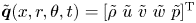 $\tilde {\boldsymbol {q}}(x,r,\theta ,t)=[\tilde {\rho } \ \tilde {u} \ \tilde {v} \ \tilde {w} \ \tilde {p}]^\textrm {T}$ includes density, streamwise, radial and azimuthal velocity fluctuations, and pressure fluctuations. The linear operator
  $\boldsymbol {L}$ is a function of the mean fluid quantities
  $[\bar {\rho } \ U \ V \ W \ P]^\textrm {T}$ and the spatial/temporal derivatives. The flow is considered locally parallel, and only the streamwise component of the mean velocity is considered. Assuming Fourier-transformed variables in time and in the streamwise direction, the response vector can be written as
 \begin{equation} \boldsymbol{\tilde{q}}(x,r,\theta,t)= \boldsymbol{\hat{q}}(r,\theta)\,\mathrm{e}^{-\mathrm{i}\omega t + \mathrm{i}\alpha x}, \end{equation}
with  $\omega$ and
  $\alpha$ the frequency and streamwise wavenumber. Under these assumptions, manipulation of the Navier–Stokes equations allows us to write a single equation for the pressure in the flow:
 \begin{equation} \frac{1}{r} \frac{\partial}{\partial r} \left( r \frac{\partial \hat{p}}{\partial r} \right) + \frac{1}{r^2} \frac{\partial^2 \hat{p}}{\partial \theta^2} - \hat{f} \frac{\partial \hat{p}}{\partial r} - \hat{g} \frac{1}{r^2} \frac{\partial \hat{p}}{\partial \theta} - \hat{h} \hat{p} = 0, \end{equation}
where the coefficients  $\hat {f}, \hat {g}, \hat {h}$ are given by
 \begin{gather} \hat{f}(r,\theta)= \frac{2\alpha}{\alpha U - \omega}\frac{\partial U}{\partial r} + \frac{1}{\bar{\rho}}\frac{\partial \bar{\rho}}{\partial r}- \frac{1}{\gamma P}\frac{\partial P}{\partial r}, \end{gather}
 \begin{gather}\hat{g}(r,\theta)= \frac{2\alpha}{\alpha U - \omega}\frac{\partial U}{\partial \theta} + \frac{1}{\bar{\rho}}\frac{\partial \bar{\rho}}{\partial \theta}- \frac{1}{\gamma P}\frac{\partial P}{\partial \theta}, \end{gather}
 \begin{gather}\hat{h}(r,\theta)=\alpha^2-\frac{\bar{\rho} ( \alpha U - \omega)^2 }{\gamma P}, \end{gather}
and the radial/azimuthal derivatives of the mean pressure are also considered, in order to account for the effect of the shock cells in the flow. Considering a  $2{\rm \pi} /N$ periodicity of the mean flow in the azimuthal direction (with
  $N$ an integer related to the number of jets in the azimuthal symmetry), we can apply Floquet theory, which considers the response to have the shape
 \begin{equation} \hat{p}(r,\theta) = p(r,\theta)\,\mathrm{e}^{\mathrm{i}\mu\theta}. \end{equation}
Under this assumption, solutions of (2.3) can be obtained in a subsection of the periodic azimuthal domain and extended to the entire domain via (2.7), reducing the computational cost. Thus, (2.3)–(2.6) can be rewritten as
 \begin{equation} \frac{1}{r} \frac{\partial}{\partial r} \left( r \frac{\partial p}{\partial r} \right) + \frac{1}{r^2} \frac{\partial^2 p}{\partial \theta^2} - f \frac{\partial p}{\partial r} - g \frac{1}{r^2} \frac{\partial p}{\partial \theta} - h p = 0, \end{equation}
with
 \begin{gather} f(r,\theta)= \frac{2\alpha}{\alpha U - \omega}\frac{\partial U}{\partial r} + \frac{1}{\bar{\rho}}\frac{\partial \bar{\rho}}{\partial r}- \frac{1}{\gamma P}\frac{\partial P}{\partial r}, \end{gather}
 \begin{gather}g(r,\theta)= \frac{2\alpha}{\alpha U - \omega}\frac{\partial U}{\partial \theta} + \frac{1}{\bar{\rho}}\frac{\partial \bar{\rho}}{\partial \theta}- \frac{1}{\gamma P}\frac{\partial P}{\partial \theta} - 2\mathrm{i}\mu, \end{gather}
 \begin{gather}h(r,\theta)=\alpha^2-\frac{\bar{\rho} ( \alpha U - \omega )^2 }{\gamma P}+\frac{\mu^2}{r^2}+\mathrm{i} \left( \frac{2\alpha}{\alpha U - \omega}\frac{\partial U}{\partial \theta} + \frac{1}{\bar{\rho}}\frac{\partial \bar{\rho}}{\partial \theta} - \frac{1}{\gamma P}\frac{\partial P}{\partial \theta} \right) \frac{\mu}{r^2} . \end{gather}
 Following Lajús et al. (Reference Lajús, Sinha, Cavalieri, Deschamps and Colonius2019), we can substitute (2.9)–(2.11) into (2.8), and isolate the terms multiplying different powers of  $\alpha$. Thus, an eigenvalue problem in discretised form can be written as
 \begin{equation} \begin{bmatrix} O & I & O \\ O & O & I \\ -\boldsymbol{F}_0 & -\boldsymbol{F}_1 & -\boldsymbol{F}_2 \end{bmatrix} \begin{bmatrix} p \\ \alpha p \\ \alpha^2 p \end{bmatrix} = \alpha \begin{bmatrix} I & O & O \\ O & I & O \\ O & O & \boldsymbol{F}_3 \end{bmatrix} \begin{bmatrix} p \\ \alpha p \\ \alpha^2 p \end{bmatrix}. \end{equation}
 In the expression above, the eigenvalue  $\alpha$ indicates both the growth rate and the streamwise wavenumber of the different waves supported by the flow. The eigenfunction
  $p(r,\theta )$ spans half of the cross-plane, and is fed into (2.7) to recover the disturbances in the entire cross-plane. The operators
  $\boldsymbol {F}_0$,
  $\boldsymbol {F}_1$,
  $\boldsymbol {F}_2$ and
  $\boldsymbol {F}_3$ are defined using the discretised azimuthal and radial derivative operators and by the mean quantities. For the present analysis, the mean streamwise velocity is taken from experiments at a given axial station, and mean pressure and density are obtained using a Crocco–Busemann approximation based on isentropic relations, and a spatial integration method (Van Oudheusden et al. Reference Van Oudheusden, Scarano, Roosenboom, Casimiri and Souverein2007). The domain is discretised using Fourier–Chebyshev in azimuth and radius, and the numerical mapping used by Bayliss & Turkel (Reference Bayliss and Turkel1992) is also applied in the radial direction, in order to obtain a higher number of points closer to the jets’ shear layers. Equation (2.12) is solved numerically using sparse matrices to reduce the computational cost. Boundary conditions are defined as in Gudmundsson (Reference Gudmundsson2009) at the centreline, such that
 \begin{equation} \left[ r^2\frac{\partial^2 p}{\partial r^2} + r\frac{\partial p}{\partial r} - \mu^2 p \right]_{r\to0} = 0, \end{equation}
but considering the boundary condition  $\partial p / \partial r =0$ at the centre of the coordinate system, used by Lajús et al. (Reference Lajús, Sinha, Cavalieri, Deschamps and Colonius2019), does not lead to perceivable changes in the eigenvalues and eigenfunctions. Dirichlet boundary conditions (
 $p=0$) are applied in the computational far field. No reflections close to the artificial boundaries were observed in the relevant modes due to their sharp amplitude decay in the radial direction (Michalke Reference Michalke1965). Results are also virtually insensitive to changes in the position of application of far-field boundary conditions for the cases studied herein.
We focus on the analysis of a twin-jet system, operating at  $\textrm {NPR}=5.0$. The mean velocity field is considered to be axisymmetric in both jets, since only the plane containing both centrelines is available from the PIV data. The velocity field in the region
  $1.5 \leq y/D \leq 4$ is obtained from experimental data, leading to a single-jet mean flow profile
  $\hat {U}(r_j)$. This profile is extrapolated to other azimuthal angles of the single jet
  $\theta _j$ by considering axisymmetry, or
 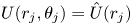 $U(r_j,\theta _j)=\hat {U}(r_j)$, where
  $(r_j,\theta _j)$ are the radial and azimuthal coordinates considered from the centre of one of the jets. Since the coordinate system for the Floquet formulation is centred at the mid-plane of the jets, this mean velocity is then interpolated into this new coordinate system. In summary, the effect of the interaction between the two jets is not considered in the present analysis, as the mean flows of the jets are considered axisymmetric; thus, all results are restricted to the axial positions before the jets start to merge. The different systems used in this problem are shown in figure 1.

Figure 1. Sketch of the coordinate system used in the present analysis. Polar coordinates  $(r,\theta )$ are associated with the centre of the twin-jet system, and
  $(r_j,\theta _j)$ are associated with the centre of a single jet. Both cross-plane (a) and full view (b) are shown.
In the present analysis, the computational domain is restricted to  $0 < r/D \leq 2.5 D_c$, and
  $0 \leq \theta < 2{\rm \pi} /N$, with
  $N=2$ for the twin-jet problem; an increase in the maximum radial distance of the domain did not lead to perceivable changes in the eigenvalues. The radial mesh is built using Chebyshev polynomials with
  $N_r=180$ collocation points, and points are distributed in an equispaced manner in azimuth, with
  $N_\theta =180$. Radial and azimuthal derivatives are taken using the algorithms described in Weideman & Reddy (Reference Weideman and Reddy2000). The the distance between the centre of the coordinate system and the centre of the jets is
  $D_c/2=1.5 D$, as in the experiments.
3. Experimental methodology
In this paper, we revisit the PIV data presented by Bell et al. (Reference Bell, Cluts, Samimy, Soria and Edgington-Mitchell2021), and the reader can refer to this previous work for more details of the experimental set-up. The jet issues from a converging nozzle of diameter  $D=10$ mm, operating at
  $\textrm {NPR}=5.0$. The distance between the centres of the nozzles is
  $D_c=3D$. Acoustic data were acquired at a distance of
  $23D$ from the origin of the twin-jet system, with a single GRAS type 46BE 1/4
 $''$ preamplified microphone at the internozzle plane. The acoustic data were acquired at a sample rate of 250 kHz, with a National Instruments DAQ, and the Welch method was performed using 2048 samples with 75
  $\%$ overlap. A Hanning window was also used to minimise spectral leakage. The spectrum is shown in figure 2, where a screech tone can be identified around
  $St_{screech}=\omega _{screech} D / (2 {\rm \pi}U_j)=0.19$, where
  $U_j$ is the ideally expanded jet velocity.

Figure 2. Power spectral density from the acoustic data of the  $\textrm {NPR}=5.0$ screeching jet. The screech tone is clearly identified around
  $St=0.19$.
Roughly 9000 PIV velocity fields (which include both streamwise and lateral velocities) were obtained in the  $x$–
$x$– $y$ plane in order to evaluate the streamwise development of both jets. The average of these fields was used to provide the mean flows for the stability analysis and to compute the velocity fluctuations for the POD. In order to consider the symmetry of the problem, we follow an approach similar to that of Sano et al. (Reference Sano, Abreu, Cavalieri and Wolf2019), defining even and odd parts of the streamwise velocity field as
 \begin{gather} u_e(x,y,t)=\frac{u(x,y,t)+u(x,-y,t)}{2}, \end{gather}
 \begin{gather}u_o(x,y,t)=\frac{u(x,y,t)-u(x,-y,t)}{2}, \end{gather}
and equivalently for the lateral velocity  $v$. This allows POD modes to be computed with half of the experimental domain, reducing the computational cost and enhancing convergence. It is important to note that only modes that are not antisymmetric regarding the
  $x$–
$x$– $y$ plane can be captured with the present experimental set-up;
  $x$–
$x$– $y$ antisymmetric modes will have zero amplitude in this PIV plane. Following Rodríguez et al. (Reference Rodríguez, Jotkar and Gennaro2018), the different modes in the twin-jet system can be classified using the nomenclature
  $m$XY, where
  $m$ is the dominant azimuthal wavenumber of the disturbance in each jet, and X and Y are related to the symmetry around the
  $y$ and
  $z$ axes, which are also connected to the Floquet coefficient
  $\mu$ as shown in table 1. Thus, modes related to azimuthal wavenumber
  $m=0$ (0S and 0A) and those following the symmetry
  $m$SS and
  $m$SA can potentially be identified among the POD modes. In all these cases, the velocities of each mode will follow the combination
  $q_{SS}=[u_e v_o]^\textrm {T}$ for the SS modes and
  $q_{SA}=[u_o v_e]^\textrm {T}$ for the SA modes.
Table 1. Symmetry of the different modes in the twin-jet system.

Proper orthogonal decomposition (Berkooz, Holmes & Lumley Reference Berkooz, Holmes and Lumley1993; Taira et al. Reference Taira, Brunton, Dawson, Rowley, Colonius, McKeon, Schmidt, Gordeyev, Theofilis and Ukeiley2017, Reference Taira, Hemati, Brunton, Sun, Duraisamy, Bagheri, Dawson and Yeh2020) is a modal analysis technique that decomposes a flow into an optimal set of functions ranked by their kinetic energy. Considering the large number of velocity fields, the snapshot method (Sirovich Reference Sirovich1987) was chosen for the present analysis. Thus, POD can be applied to both SS and SA datasets, which are orthogonal by construction, such that the autocovariance matrix of the SS modes is given by
 \begin{equation} \boldsymbol{R}_{SS}=\boldsymbol{Q}_{SS}^T \boldsymbol{Q}_{SS}, \end{equation}
where the columns of the matrix  $\boldsymbol {Q}_{SS}$ are built by stacking the velocity vectors for each snapshot. The POD modes are obtained by solving the eigenvalue problem
 \begin{equation} \boldsymbol{R}_{SS} \mathbf{\xi}_{SSj} = \sigma_{SSj} \mathbf{\xi}_{SSj}, \end{equation}
where the eigenvalues  $\sigma _{SSj}$ are ordered in descending order, each of them related to the energy of the modes. Since no flow reconstruction is attempted in the present work, scaling factors and integration weights are not considered in the analysis; thus, the eigenfunctions
  $\mathbf {\xi }_{SSj}$ are linked to the temporal coefficients of each mode by
  $a_{SSj}(t)=\mathbf {\xi }_{SSj}$, and are related to the POD mode shapes by
  $\mathbf {\phi }_{SSj}=\boldsymbol {Q}_{SS}\mathbf {\xi }_{SSj}$. The equivalent decomposition was also performed for the SA modes.
As highlighted by Taira et al. (Reference Taira, Brunton, Dawson, Rowley, Colonius, McKeon, Schmidt, Gordeyev, Theofilis and Ukeiley2017), POD modes contain a mix of frequencies, which can cloud the analysis. Still, considering that the jet is screeching at a single frequency for this case, the POD mode related to the feedback loop at the screech frequency is likely to dominate the field (Edgington-Mitchell et al. Reference Edgington-Mitchell, Oberleithner, Honnery and Soria2014b, Reference Edgington-Mitchell, Jaunet, Jordan, Towne, Soria and Honnery2018; Jaunet, Collin & Delville Reference Jaunet, Collin and Delville2016; Edgington-Mitchell et al. Reference Edgington-Mitchell, Wang, Nogueira, Schmidt, Jaunet, Duke, Jordan and Towne2021).
4. Results
4.1. Mean flows
The temporal averages of the streamwise ( $U$) and lateral (
 $V$) velocities, normalised by the ambient speed of sound, are shown in figure 3. At such high NPR, the flow issues from the nozzle at unit Mach number, and experiences a strong expansion, which leads to an acceleration in the near-nozzle region. A large Mach disk is generated at the first shock cell, and the typical shock-cell pattern is formed further downstream, as expected for underexpanded jets. The mean flow follows the expected symmetry, with the streamwise velocity keeping an ‘even’ (
 $U_{(y>0)}=U_{(y<0)}$) configuration, opposed to the lateral velocity, which displays an ‘odd’ (
 $V_{(y>0)}=-V_{(y<0)}$) symmetry. Any deviations from this behaviour are due to small alignment errors or by diffraction of the laser sheet by the Mach disk of the bottom jet; still, anomalies due to these effects are minor.

Figure 3. Streamwise (a) and lateral (b) mean flows from PIV experiments. The magnitudes of both velocity components at the system centreline ( $y=0$) are also shown in (c) and the mean streamwise velocities at several axial stations analysed in this work are shown in (d). All fields are normalised by the ambient velocity of sound.
These mean velocity fields were used to provide slices of the mean flow for the spatial stability analysis. Considering that no cross-plane information was available from the experiments, each jet was considered to be axisymmetric, and the velocities at the cross-planes were obtained by rotation of the mean fields around each jet axis, and the ‘even’ symmetry was imposed in the streamwise velocity field. The hypothesis of axisymmetric jets may be valid for axial stations prior to the merging point of the system, which can be estimated by the axial station where the mean streamwise velocity starts to increase considerably at the  $x$–
$x$– $z$ symmetry plane. Figure 3(c) shows that the lateral velocity is zero at the centreline of the system (
 $y/D=0$). Since the symmetry of this velocity component requires zero velocity in the
  $x$ axis, this confirms that the PIV system is aligned and that the data are well converged. The streamwise velocity is also very close to zero at
  $y=0$ up to
  $x/D=5$, supporting the hypothesis that the effect of the interaction between the jets on the mean fields is small up to that position, and that the jets had not merged before that station. Further downstream, as the jets start to merge, the amplitude of the mean velocity starts to increase considerably. The axisymmetric assumption is also supported by the symmetry of sample streamwise velocity fields, shown in figure 3(d). In these fields, the impact of the Mach disk is also clearly seen around the centreline of the jet, where a second shear layer is observed. The effect of the shock-cell structure is captured in figure 3(d), where the mean flow is shown to vary non-monotonically for increasing
  $x/D$. These plots altogether suggest that the axisymmetric assumption is valid up to
  $x/D=5$; thus, LSA was performed for
  $x/D\leq 5$. Also, we avoided regions close to the Mach disk, were new unstable modes may appear due to the formation of an inner shear layer (Edgington-Mitchell, Honnery & Soria Reference Edgington-Mitchell, Honnery and Soria2014a). A sample of the mean flow used in the LSA for
  $x/D=4$ and its respective radial and azimuthal derivatives are shown in figure 4; in all cross-plane visualisations, the
  $z$ axis is labelled as
  $-z/D$ to account for an observer facing the jets from the positive
  $x$ axis (see figure 1).

Figure 4. Sample mean flow interpolated into the computational mesh for stability analysis (a) and its respective radial  $\partial U / \partial r$ (b) and azimuthal
  $\partial U / \partial \theta$ (c) derivatives (
 $x/D=4$). Modes are normalised by the ambient speed of sound.
4.2. Proper orthogonal decomposition
The POD spectra for both SS and SA modes are shown in figure 5. As in Edgington-Mitchell et al. (Reference Edgington-Mitchell, Oberleithner, Honnery and Soria2014b) and Bell et al. (Reference Bell, Soria, Honnery and Edgington-Mitchell2017), the first two POD modes have similar energy, and they sum up to around  $11.4\,\%$ of the energy of the SS field (or
  $6\,\%$ of the total energy of the flow). The third mode has also a significant separation from the other suboptimal modes and has no correspondent pair; for the present case, its energy is around half of the total energy of the first pair. For the SA modes, the spectrum shows dominance of a single mode, which contains around
  $5\,\%$ of the energy of the SA field, and
  $2.4\,\%$ of that of the total field. Similarly to the third POD SS mode, this mode has no correspondent pair. As usual in turbulent flows, a large number of modes is necessary to account for most of the kinetic energy of the jets, but a clear separation in energy of the first few modes can point to dominant physical mechanisms at play in the flow (Jaunet et al. Reference Jaunet, Collin and Delville2016). Considering that the overall energy of the SS mode is around
  $10.4\,\%$ greater than the SA mode, the dynamics involving modes with the SS symmetry is expected to overrule the ones related to SA modes.

Figure 5. The POD spectra for both SS (a) and SA (b) modes. Blue symbols (and left-hand  $y$ axis) depict the fraction of the total energy held by each mode and orange lines (right-hand
  $y$ axis) show the cumulative energy as a function of the number of modes. All percentages are related to the total energy associated with each symmetry (SS or SA). The total energy of SS modes is
  $10.4\,\%$ greater than the total energy of SA modes.
The shapes of the dominant POD SS modes are shown in figure 6. Similar to Edgington-Mitchell et al. (Reference Edgington-Mitchell, Oberleithner, Honnery and Soria2014b) and Bell et al. (Reference Bell, Soria, Honnery and Edgington-Mitchell2017), these modes represent coherent structures in the flow, with their spatial support related to the different waves present in the jets. The two first modes display an oscillatory behaviour in both streamwise and lateral velocity fields, which are symmetric and antisymmetric regarding the  $x$–
$x$– $z$ plane of the twin-jet system by construction. This is highlighted by the zero amplitude of the modes at
  $y/D=0$ for the lateral velocity and non-zero amplitudes at the same position for the streamwise velocity. Figure 6(a,c) also shows that each jet is dominated by
  $m=1$ disturbances, since the amplitudes of the modes at the centreline of each jet are close to zero, with phase-shifted disturbances on both sides of a jet, which precludes the presence of an
  $m=0$ mode. Also, figure 6(b,d) shows that the lateral velocity is non-zero at the jet centreline in these modes, which would not be the case if
  $m>1$. The two first modes also have a strong signature of waves with support outside the jets, which is particularly strong in the interjet region. These waves can be related either to a coupling of the KH modes of the two jets or to upstream waves generated by this system. As expected in the analysis of flows with temporally coherent oscillatory motions, the shape of the second mode is similar to that of the first mode with a change in streamwise phase, which can be seen more clearly for the streamwise velocity. Due to the presence of both downstream- and upstream-travelling modes, the phase offset is not immediately apparent from visual inspection. However, a consideration of the mode coefficients provides a robust means to demonstrate that these modes are a pair representing a single physical mechanism (a travelling mode associated with the screech phenomenon) in the flow.

Figure 6. Three dominant POD modes for the SS field. Both streamwise (a,c,e) and lateral (b,d,f) velocities are shown. Modes 1 and 2 (a–d) seem to form a pair, and mode 3 (e,f) has no associated pair. All fields are normalised by their maximum. (a) POD-SS mode 1 (u), (b) POD-SS mode 1 (v), (c) POD-SS mode 2 (u), (d) POD-SS mode 2 (v), (e) POD-SS mode 3 (u) and (f) POD-SS mode 3 (v).
Unlike the two first modes, the third POD SS mode varies slowly in the streamwise direction, and peaks further downstream. This mode has a strong signature at the shear layer and in positions slightly further away from the centre of the jet in the radial direction, with very low amplitudes at the centreline. The same is true for the lateral velocity, with the difference that this field is antisymmetric with respect to each jet axis. The overall shape of this mode is similar to the one analysed by Weightman et al. (Reference Weightman, Amili, Honnery, Soria and Edgington-Mitchell2018); in that previous work, the authors attributed this mode to a ‘shear-layer unsteadiness’ (or shear thickness mode), whose main effect is the amplitude modulation of the instability waves. The same characteristics are shared by the first POD SA mode (omitted here for conciseness).
In order to confirm the pairing between the two first modes, an analysis of the temporal coefficients resulting from POD is necessary. As shown by Oberleithner et al. (Reference Oberleithner, Sieber, Nayeri, Paschereit, Petz, Hege, Noack and Wygnanski2011), coefficients of POD modes related to a single travelling mode of the jet should fall within a circle in phase space. The phase portrait of the first three POD SS modes is shown in figure 7(a). The three-dimensional portrait resembles an ellipsoid shell cut in half, aligned with the  $a_3$ axis; to analyse this result in detail, we define a cycle radius
  $r_{12}=\sqrt {a_1^2+a_2^2}$, which represents the relative magnitude of the cycle represented by the
  $a_1$ and
  $a_2$ modes. From figure 7(b), which shows the dependence of
  $r_{12}$ with
  $a_3$, it can be inferred that the third mode modulates the amplitude of the cycle involving modes 1 and 2, with low values of
  $a_3$ associated with a smaller cycle radius, as also observed by Weightman et al. (Reference Weightman, Amili, Honnery, Soria and Edgington-Mitchell2018). This is also in line with recent studies of the effect of streaks on the KH instability mechanism (Marant & Cossu Reference Marant and Cossu2018; Lajús et al. Reference Lajús, Sinha, Cavalieri, Deschamps and Colonius2019; Nogueira & Cavalieri Reference Nogueira and Cavalieri2021), which have shown that such elongated structures can have a stabilising/destabilising effect on the KH mode. Figure 7(c) shows the phase portrait of modes 1 and 2, for restricted values of
  $a_3$ (
 $|a_3-0.02|<0.01$). Clearly, most values of
  $(a_1,a_2)$ fall within a single circle, confirming that modes 1 and 2 form a cycle in phase space.

Figure 7. Three first POD SS coefficients forming an ellipsoid (a). Amplitude of the  $a_1$–
 $a_2$ cycle (
 $r_{12}=\sqrt {a_1^2+a_2^2}$) as a function of
  $a_3$ (b). Phase portrait of modes
  $a_1$ and
  $a_2$ for
  $|a_3-0.02|<0.01$ (c).
Thus, the overall picture depicted by the POD is a mode pair that represents the in-phase waves of the system, which include the KH mode and the upstream-travelling wave (which are responsible for closing the resonance loop), as in Edgington-Mitchell et al. (Reference Edgington-Mitchell, Wang, Nogueira, Schmidt, Jaunet, Duke, Jordan and Towne2021). This resonance loop is modulated by the third POD SS mode (shear thickness mode/streak), such that small cycle amplitudes are found for low values of  $a_3$. Considering the lack of cross-plane information, little can be said about this third mode; thus subsequent analysis will focus on the first two modes, which are associated with the generation of screech tones. Following the formulation of Jaunet et al. (Reference Jaunet, Collin and Delville2016) and Edgington-Mitchell et al. (Reference Edgington-Mitchell, Jaunet, Jordan, Towne, Soria and Honnery2018), we define the screeching mode from the first mode pair as
 \begin{equation} \mathbf{\zeta}(x,y,t) = (\mathbf{\phi}_{SS1} + \mathrm{i} \mathbf{\phi}_{SS2})\,\mathrm{e}^{-\mathrm{i} \omega_s t}, \end{equation}
where  $\omega _s$ is the screech frequency. In order to identify the different waves that compose this mode, a spatial Fourier transform was applied in the streamwise direction. Such analysis not only allows us to decompose this structure into the different wave components, but also to have a first evaluation of the radial structure of these waves. The wavenumber spectra from the spatial Fourier transform of both velocity fields are shown in figure 8. The Fourier transform was performed with
  $n_{fft}=4096$ points, and the signal was zero-padded for
  $N_x>1036$ in order to provide a better visualisation of the most energetic wavenumbers in the flow. This process does not lead to significant changes in the spectrum, and allows for a higher resolution in wavenumber. As expected, a strong signature of the KH mode is observed for both velocity components at positive wavenumbers (around
  $k_x D=1.8$), as in Edgington-Mitchell et al. (Reference Edgington-Mitchell, Wang, Nogueira, Schmidt, Jaunet, Duke, Jordan and Towne2021). The presence of upstream-travelling waves is also seen in the negative wavenumber region for both velocity components. The wavenumber of these waves is in good agreement with the wave-interaction theory proposed by Tam & Tanna (Reference Tam and Tanna1982): the blue dashed line indicates the wavenumber energised by the interaction between the KH mode and the shock-cell structure, which matches the peak wavenumber of the upstream waves.

Figure 8. The POD SS wavenumber spectra for both streamwise (a) and lateral (b) velocity components. Blue line depicts the wavenumber energised by the interaction between the KH mode (peak of both spectra) and the shock-cell structure.
The effect of the coupling between the two jets can be seen clearly in both figures 6 and 8. Overall, the presence of a neighbouring jet induces higher streamwise velocity amplitudes in the interjet region, and a cancellation of lateral velocity due to the symmetry of the SS mode. Even though POD is very efficient in extracting the most energetic spatially coherent structure from this turbulent flow, it does not provide any reasoning for this specific coupling. Also, the shapes of the modes are restricted by the PIV plane used in the present analysis, and the overall structure of the coupled mode for this twin-jet system is still unclear. In the next section, a spatial LSA around an extrapolated mean flow from the experiments is conducted in order to explore the conditions for such coupling.
4.3. Spatial LSA
As mentioned in § 4.1, the LSA is focused on the region between the end of the inner shear layer generated by the Mach disk and the merging point of the twin-jet system. We start the analysis by introducing the shapes of the different KH modes related to azimuthal wavenumber  $m=1$ predicted by this tool. Their overall stability characteristics are also described, which includes an analysis of the dependence of growth rates and phase velocities with frequency and axial position. We then proceed to the description of the upstream-travelling waves predicted by the same analysis, with focus on the bands of existence of these waves in the frequency–wavenumber space. The shapes of the modes predicted by the LSA are also compared with those from the POD wavenumber spectrum in order to provide further validation of the mechanism at play in this system. As mentioned previously, the LSA was performed in the interval
  $3 \leq x/D \leq 5$ in order to avoid the merging region of the jets (which could not be directly used in the mean flow extrapolation) and the region around the Mach disk. Still, it will be seen that the region in which the analysis was performed is representative of the resonance phenomenon at play, finding a correspondence to the waves found in the POD analysis.
All the modes of this section are obtained as in Rodríguez et al. (Reference Rodríguez, Jotkar and Gennaro2018). In summary, the spectrum containing eigenmodes related to different symmetries and azimuthal wavenumbers is obtained as a function of frequency, and the relevant modes are extracted for the analysis. For the streamwise stations analysed herein, there are usually three unstable modes for each value of  $\mu$: two related to
  $m=\pm 1$ disturbances (which are dominant) and another related to
  $m=0$ disturbances, which does not find an equivalence with the POD modes. Other KH modes (with higher
  $m$) are either stable or just marginally unstable. Considering the size of the problem, only a few eigenvalues are obtained using the function eigs in Matlab. The shift (the position of the spectrum around which eigenvalues are sought) is chosen to be close to wavenumbers related to the usual phase velocity of KH disturbances (Michalke Reference Michalke1970). Thus, the most unstable modes are obtained for all frequencies and axial stations analysed, and the correct symmetries are isolated after post-processing. The same approach is undertaken for the upstream waves, but a different shift is chosen for this case, requiring another run of eigs. The complete spectrum of the twin-jet system is very large, and can only be obtained by parts. Still, there are only two regions of interest in the spectrum for the present study: the regions related to the KH and guided jet modes. In this section, we focus on the analysis of both waves, whose characteristics (like growth rates, wavenumbers and range of existence) will shed light on the possible reasons for symmetry locking of the screech mode in this configuration.
4.3.1. The KH mode
In order to identify all modes related to the KH instability, (2.12) is solved for several streamwise positions ( $x/D$) and Strouhal numbers around the screech frequency (
 $St_{screech}=0.19$). In this whole range, the modes with highest growth rates are related to a combination of azimuthal wavenumbers
  $m=\pm 1$ between the two jets. The pressure fields of the different modes for
  $x/D=4$ and
  $St=0.19$ are shown in figure 9. Overall the modes are similar to those found by Rodríguez et al. (Reference Rodríguez, Jotkar and Gennaro2018), and they follow the symmetry described in table 1. The different symmetries of the modes lead to regions of zero amplitude in the field, especially in the
  $x$–
$x$– $y$ plane (for
  $y=0$, or the
  $z$ axis) and the
  $x$–
$x$– $z$ plane (for
  $z=0$, or the
  $y$ axis). These four different modes can be used to represent disturbances associated with the KH instability in the locally parallel framework; a linear combination of these modes can be compared with results from experiments such as the POD modes analysed in § 4.2. Each mode is also associated with a complex wavenumber
  $\alpha =\alpha _{kh}+\mathrm {i} \alpha _i$, where
  $\alpha _{kh}$ denotes the streamwise wavenumber of the KH disturbance and
  $\alpha _i$ represents the spatial growth rate. In the absence of resonance, the mode with the highest spatial growth rate would be expected to dominate the hydrodynamic field. In a resonant system, the spatial growth of the downstream-propagating disturbance remains an important element in determining the overall gain of a particular feedback mode. However, as is shown in the following section, it is not necessarily the sole determinant.

Figure 9. Real part of the pressure field of KH modes related to azimuthal wavenumber  $m=1$,
  $St=0.19$ and
  $x/D=4$. The eigenmodes in the cross-plane can be directly associated with the different symmetries allowed in the problem. Modes (a) 1SS (
 $\mu =0$), (b) 1AA (
 $\mu =0$), (c) 1SA (
 $\mu =1$) and (d) 1AS (
 $\mu =1$).
Figure 10(a) shows the growth rates of the different KH modes for  $x/D=4$ and Strouhal numbers around the screech frequency. Overall, the growth rates of all modes peak around
  $St=0.14$ and decay for higher frequencies. The plot also shows a slight dominance of the 1SA mode over the other modes in this range of frequencies. The streamwise wavenumbers of the disturbances, shown in figure 10(b), follow a single line, which indicates that all modes have roughly the same phase velocity (except for the 1SA mode at very low frequencies); since the resonance loop is strongly affected by this quantity (Raman Reference Raman1998; Edgington-Mitchell et al. Reference Edgington-Mitchell, Wang, Nogueira, Schmidt, Jaunet, Duke, Jordan and Towne2021), this suggests that any of these modes should be equally able to close resonance in the present system. Figure 10(c,d) confirms that these features remain for the different streamwise positions analysed, with a consistent dominance of the 1SA mode, and very little change in the streamwise wavenumber of the different modes. Since the experimental profile was used in the analysis, which displays strong oscillations due to the presence of the shock-cell structure, it is natural to expect variations in the eigenvalue
  $\alpha$, as seen in figure 10(c,d). Still, these results show that these trends are robust, and the modes are qualitatively similar at different axial positions.

Figure 10. Growth rates of KH modes related to  $m=1$ for
  $x/D=4$ as a function of Strouhal number (a) and their respective streamwise wavenumbers (b). (c,d) Same quantities as a function of streamwise station for
  $St=0.19$. (a,c) Growth rates and (b,d) Wavenumbers.
The analysis of the KH modes shows that the growth rates and streamwise wavenumbers of all modes are very similar for a given  $St$ and
  $x/D$. Comparing the wavenumbers of figure 10(b,d) with the positive part of the spectra shown in figure 8 leads to a very good agreement (within
  $3.5\,\%$ of the peak wavenumber for
  $St=0.19$); thus, LSA performed in these positions is able to capture some of the key characteristics of this structure. The KH mode is one of the key parts of the resonance phenomenon, but a complete description of screech can only be performed with an analysis of the upstream-travelling wave, which is responsible for closing the resonance mechanism. This is performed in the next section.
4.3.2. The upstream-travelling mode
Screech is a resonant phenomenon characterised by four processes and two waves travelling in opposite directions: the KH (downstream-travelling) wave and an upstream-travelling wave. Recent works (Gojon et al. Reference Gojon, Bogey and Mihaescu2018; Edgington-Mitchell et al. Reference Edgington-Mitchell, Jaunet, Jordan, Towne, Soria and Honnery2018; Mancinelli et al. Reference Mancinelli, Jaunet, Jordan and Towne2019) have shown that resonance might be closed by an upstream-travelling guided jet mode, instead of an acoustic wave. Thus, an analysis of the spatial structure and the bands of existence of these waves in the frequency–wavenumber domain is a key part of the analysis of the resonant cycle. We analyse these features in the present section.
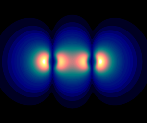
Figure 11 shows the real part of the pressure field associated with the guided jet modes for  $x/D=4$ and
  $St=0.19$ (1SS and 1AS) and
  $0.20$ (1AA and 1SA). As in the KH mode, the symmetry of the problem allows for the existence of four different modes, following the same characteristics of this downstream-travelling wave (summarised in table 1), thus inheriting the same classification. Comparing the radial structure of the waves shown in figure 11 with those in Gojon et al. (Reference Gojon, Bogey and Mihaescu2018), it becomes clear that these waves are of first radial order, displaying a single node at the centre of the jets. As in the previous case, the combination of different values of
  $m=\pm 1$ between the two jets leads to four modes that may be used to represent the upstream-travelling waves in the real system. As shown by Tam & Hu (Reference Tam and Hu1989), Towne et al. (Reference Towne, Cavalieri, Jordan, Colonius, Schmidt, Jaunet and Brès2017), Gojon et al. (Reference Gojon, Bogey and Mihaescu2018) and Edgington-Mitchell et al. (Reference Edgington-Mitchell, Jaunet, Jordan, Towne, Soria and Honnery2018), these waves are spatially neutral, and they form a saddle with a neutral soft-duct mode in the eigenvalue spectrum, generating a stable upstream-travelling wave with a very similar spatial structure, and this is also the case for the twin-jet system. The stable wave is shown in figure 11(b) for the 1AA mode, since the bands of existence of the neutral wave for this symmetry are very small, hampering its identification.

Figure 11. Real part of the pressure field of upstream modes for  $x/D=4$ and
  $St=0.19$ (1SS, 1AS) and
  $0.20$ (1AA, 1SA). The stable upstream-travelling mode is shown for the 1AA case. Modes (a) 1SS (
 $\mu =0$,
  $St=0.19$), (b) 1AA (
 $\mu =0$,
  $St=0.20$), (c) 1SA (
 $\mu =1$,
  $St=0.20$) and (d) 1AS (
 $\mu =1$,
  $St=0.19$).
The frequency range of existence of the upstream modes is explored in figure 12 for the different symmetries and three different axial stations. This frequency range is defined by the Strouhal number between the point at which the waves become propagative (represented by the black dashed lines) and the saddle point (the frequency at which this neutral mode encounters the soft-duct mode, generating the stable wave). As in the KH case, the characteristic wavenumbers of these waves change slightly as we go downstream, which is a consequence of the mean velocity variations induced by the shock-cell structure: since both  $x/D=3$ and
  $5$ are close to minima of the shock-cell structure, the magnitude of the mean velocity is smaller (as shown in figure 3d), leading to higher values of Strouhal number for the branch and saddle points of the guided jet mode (see Gojon et al. Reference Gojon, Bogey and Mihaescu2018). On the other hand,
  $x/D=4$ is close to a maximum, explaining the lower values of
  $St$ in figure 12(b,e). The first feature observed in these plots is the very small range of frequencies in which the 1AA and 1SA modes can be identified. This happens consistently over all the axial positions analysed, with
  $x/D=5$ being the station with the largest range of frequencies in which these modes are active. By comparison, the bands of existence of the 1SS and 1AS modes are much larger for all axial stations analysed, which can also be seen more clearly for
  $x/D=5$. Figure 12 also shows that the neutral modes are active in a range of frequencies reasonably close to the screech frequency (
 $St_{screech}=0.19$), which suggests that the guided jet mode is the wave responsible for closing the resonance loop in the twin-jet case.

Figure 12. Wavenumber of the upstream-travelling modes related to  $m=1$ for
  $x/D=3,4,5$ and several Strouhal numbers. The dashed line indicates the speed of sound, which is the point where the guided jet mode becomes propagative. (a)
  $\mu =0$;
  $x/D=3$, (b)
  $\mu =0$;
  $x/D=4$, (c)
  $\mu =0$;
  $x/D=5$, (d)
  $\mu =1$;
  $x/D=3$, (e)
  $\mu =1$;
  $x/D=4$ and (f)
  $\mu =1$;
  $x/D=5$.
Altogether, the results from figures 10 and 12 help to delineate the phenomenon at play. In summary, the KH characteristics of the four possible modes are not sufficient to define a dominant coupling symmetry, since their growth rates and phase speeds are very similar to each other. On the other hand, the characteristics of the upstream-travelling wave at play in the resonance cycle change substantially among the four different symmetries. Neutral upstream modes 1SA and 1AA are barely identified in the frequency–wavenumber spectrum before they become stable, while neutral modes 1SS and 1AS have a larger region of existence. Thus, the latter two modes have a larger frequency range in which resonance can be closed. Considering that one of the key elements of screech is the interaction between KH modes and shocks transferring energy to the upstream waves (Tam & Tanna Reference Tam and Tanna1982; Shen & Tam Reference Shen and Tam2002; Edgington-Mitchell et al. Reference Edgington-Mitchell, Wang, Nogueira, Schmidt, Jaunet, Duke, Jordan and Towne2021), modes 1SS and 1AS are possibly the ones closing the resonance in this case, which could lead either to a 1SS or 1AS flapping motion, or a helical motion involving a combination of the two modes. The POD modes show clearly the presence of a 1SS mode, which reduces the options to a 1SS flapping regime, or a 1SS/1AS helical motion, in which only the 1SS component is observed in the POD; the present experimental set-up cannot allow for the identification of 1AS modes, since these modes would have zero amplitudes at the measurement plane. Therefore, due to the absence of cross-plane measurements of the present dual-jet system, no strong claims about which regime is dominant can be made.
4.3.3. Comparison with structures from POD
The previous sections provided an explanation for the resonance involving the 1SS mode, highlighting the characteristics of the different waves that make this mode more likely to close the loop. In this section, we focus on a spatial comparison between the structures coming from the dominant POD modes and the 1SS waves from spatial LSA. This will provide more confidence about the nature of the waves involved in the resonance cycle. The comparison between POD and linear stability modes is performed by the computation of the streamwise and lateral velocity components from the pressure eigenfunctions of (2.12). In the present case, the comparisons are performed with the modes resulting from LSA for  $x/D=5$ and
  $St=0.2075$, which provided the best quantitative agreement with experiments, especially for the upstream wave; evaluation of other positions and frequencies led to a similar qualitative agreement.
Radial shapes of the different waves identified in the wavenumber spectrum of the leading POD mode pair were extracted at their peak wavenumbers. These can be compared with the LSA modes at certain frequencies and axial positions, and comparisons between wavenumbers can also be performed. For the present case ( $x/D=5$,
  $St=0.2075$), the comparison between the peak wavenumbers of the two waves educed from POD and those coming from LSA is shown in table 2. It is clear that wavenumbers of the different waves from both analyses are in good agreement, despite the small difference in Strouhal number. The error associated with these wavenumbers for this case is within 5 % for the KH mode, and less than 1 % for the upstream wave. Also, figures 10 and 12 show that, even though these wavenumbers may vary with axial position, this variation is not substantial within the range of frequencies and axial stations analysed, especially considering the small range of frequencies in which the guided jet mode exists.
Table 2. Peak wavenumbers of the different waves extracted from the POD wavenumber spectrum compared with the wavenumbers of the waves from LSA for  $x/D=5$ and
  $St=0.2075$.

The radial shapes of the different waves from POD and LSA are compared in figure 13. Here, only amplitudes of these modes are shown, since all modes are considered to have a single frequency and wavenumber; the radial phase information, related to the positions of peaks and nodes of the different modes, can be directly inferred from figure 13. For the KH wave, mode shapes from the POD wavenumber spectrum are more radially spread than the linear stability results, as shown in figure 13(a), which can be connected to both molecular and turbulent viscous effects; a consideration of these effects may lead to a better comparison between the modes, similar to what was observed by Pickering et al. (Reference Pickering, Rigas, Schmidt, Sipp and Colonius2020) for resolvent analysis. One should keep in mind that the LSA does not consider the spreading of the mean flow, which can also lead to KH modes that are more spread in space. Also, the relative amplitudes of the peaks are not equal, as well as the radial decay rate in the interjet region and the outer region. Still, some qualitative features are familiar: as in the POD, the LSA mode displays a second oscillation closer to the centre of the jets in the streamwise velocity, which is related to the Mach disk wake (Edgington-Mitchell et al. Reference Edgington-Mitchell, Honnery and Soria2014a), and the phase shifts of this coherent structure for different radial positions are also in agreement. A phase shift of  ${\rm \pi}$ between the interjet region and the outer region is also present in the streamwise velocity for both LSA and POD modes. The asymmetry of the mode around
  $y/D=1.5$ is also well captured, which would not be possible if a single-jet spatial stability analysis was performed. Overall, the shape of the lateral velocity, shown in figure 13(b), is even closer to the POD modes. Despite the sharper valley around
  $y/D=1.5$, the LSA was able to capture some essential features like the radial decay of disturbances and the double peak close to the centre of the jets.

Figure 13. Comparison between mode 1SS from LSA (both (a,b) KH and (c,d) upstream waves) and the dominant POD mode (extracted from the energy peaks at positive and negative wavenumbers of the spectra shown in figure 8). The LSA was computed using  $x/D=5$ and
  $St=0.2075$. All modes are normalised by their maximum amplitude.
The radial shapes of the upstream-travelling wave are shown in figure 13(c,d). A remarkable agreement between the POD mode and the LSA is observed for both velocity components: all peaks and nodes are correctly described by the LSA, the radial decay (both towards the second jet and outwards) is well captured, as well as the particular asymmetric behaviour around the centre of the jet. The same is found for the lateral velocity, where a slight mismatch in the interjet region is observed. This could be due to the absence of the mean radial velocity in the analysis, or the axisymmetric jet assumption; small deviations from that assumption are expected in the interjet region, and that could affect the shapes of the modes. Still, this level of agreement suggests that this wave is not as affected by the jet spreading and the viscous effects as the KH mode. It also suggests that the resonance loop is, indeed, closed by the guided jet mode for the twin-jet system even at such high Mach number.
The present results can also be interpreted in light of the analysis of Bell et al. (Reference Bell, Cluts, Samimy, Soria and Edgington-Mitchell2021). In that previous work, the authors identified the presence of three processes related to the coupling between the two jets. It was shown that, at  $\textrm {NPR}=5.0$, the screech tone is steady, and the flow is dominated by a single process associated with symmetric oscillations in the PIV plane (here identified as 1SS mode). Still, since no out-of-plane data were available, no conclusion about the 1AS component could be made. The present results confirm that the 1SS mode is active, and that this is a consequence of the characteristics of the upstream wave related to that symmetry. However, we show that the 1AS mode is also likely to be present, especially considering that the characteristics (phase velocity and bands of existence) of the waves with the 1AS symmetry are very close to those of the waves with the 1SS symmetry. This is also supported by the fact that different processes can be supported simultaneously in the twin-jet system, as shown by Bell et al. (Reference Bell, Cluts, Samimy, Soria and Edgington-Mitchell2021). Evaluation of the role of the 1AS mode will require an experimental campaign that includes cross-plane measurements. Measurements in the
  $r$–
$r$– $\theta$ plane will enable identification of all possible mode symmetries, and permit direct comparison of their relative energies using symmetry-imposed POD.
5. Conclusions
The present work focused on a characterisation of the twin-jet coupling operating at high Mach number and underexpanded condition. The PIV data presented in previous works (Bell et al. Reference Bell, Soria, Honnery and Edgington-Mitchell2018, Reference Bell, Cluts, Samimy, Soria and Edgington-Mitchell2021) were revisited, and a POD was performed imposing the symmetry of the problem. This confirmed the identification of a dominant regime in the flow (1SS), and modes with the dominant symmetry were generated. It was found that three modes are especially relevant in the resonant phenomenon: a mode pair related to the different waves present in the cycle, and a third mode that can be associated with a shear thickness modulation. Spatial Fourier transform of the leading POD mode pair led to the identification of two waves in the velocity field: the KH mode, which has positive wavenumber peak in the spectrum, and the upstream-travelling wave (related to the negative wavenumber peak).
The mean flow from the PIV experiments was used to perform a spatial LSA, which was designed to take advantage of the current symmetry by using Floquet theory. From the LSA, four modes associated with the KH instability mechanism were identified, each one related to a combination of azimuthal wavenumbers  $m=\pm 1$ of each jet. All four modes had similar growth rates and phase velocities for all frequencies and axial stations analysed, which provided no argument for resonance locking in any of the modes. By using LSA, we also identified four different upstream-travelling modes, following the same symmetries as the KH mode. In contrast with the KH mode, the characteristics of the upstream modes change substantially between the different symmetries, and modes related to 1SS and 1AS have a much larger range of allowable frequencies in which resonance can be closed. This result is consistent over all axial stations analysed, and the frequency range in which these modes exist is also close to the screech frequency for this case.
Finally, modes from LSA were compared to the leading POD mode pair. Overall, LSA modes led to coherent structures that are qualitatively similar to the ones found in POD, especially concerning the positions of the peaks and the phase jumps. By comparing the radial structure related to the peaks of the spatial Fourier transform of the POD mode pair, it was seen that the KH mode is qualitatively well predicted by the LSA. The shapes of the upstream waves were in close agreement, and even the details of these structures were captured by the LSA. Wavenumbers of both structures were also very close to those from the POD Fourier spectrum.
We present a method to analyse single- and twin-jet systems (and other flows with azimuthal non-uniformity) using LSA and a symmetry-imposed POD associated with a spatial Fourier transform, which has proven useful for revealing some of the characteristics of the resonance phenomenon at play. The results show the relevance of the KH mode in screech, and highlight that the characteristics of the upstream-travelling guided jet mode are an essential part of the dynamics – in this case, this wave dictates which coupling regime will be followed by the twin-jet system, being a key part of the resonance phenomenon.
Acknowledgements
The authors acknowledge Peter Jordan, Matteo Mancinelli, Vincent Jaunet, André Cavalieri, Daniel Rodríguez and Aaron Towne for fruitful discussions. We also thank Graham Bell for providing the PIV and acoustic data of the twin-jet system. The computational facilities supporting this project included the Australian NCI Facility, the partner share of the NCI facility provided by Monash University through an ARC LIEF grant and the Multi-modal Australian ScienceS Imaging and Visualisation Environment (MASSIVE).
Funding
This work was supported by the Australian Research Council through the Discovery Project scheme: DP190102220.
Declaration of interests
The authors report no conflict of interest.


