


1. Introduction
The work of Kolmogorov (Reference Kolmogorov1941a,Reference Kolmogorovb) (referred to herein as K41) proposed the existence of an inertial subrange that separates the dissipative scales from the energy-containing ones in the limit of sufficiently high Reynolds numbers. These notions were later extended to passive-scalar fields by Oboukhov (Reference Oboukhov1949) and Corrsin (Reference Corrsin1951) (referred to herein as KOC), who proposed analogous concepts to those in K41, such as local isotropy of passive-scalar fields and the existence of an inertial–convective subrange. As established by K41 and KOC, two important parameters of turbulent flows are the dissipation rates of the turbulent kinetic energy and scalar variance, respectively defined as
 \begin{equation} \langle \epsilon \rangle = 2\nu \langle s_{ij}s_{ij}\rangle, \end{equation}
and
 \begin{equation} \langle \epsilon_{\theta} \rangle = \gamma \left\langle \frac{\partial \theta}{\partial x_i} \frac{\partial \theta}{\partial x_i}\right\rangle, \end{equation}
where  $s_{ij}=\frac {1}{2}({\partial u_i}/{\partial x_j}+{\partial u_j}/{\partial x_i})$ is the fluctuating strain rate,
  $u_i$ is the velocity fluctuation,
  $\theta$ is the passive-scalar fluctuation,
  $\nu$ is the kinematic viscosity and
  $\gamma$ is the scalar diffusivity. K41 and KOC theories make use of the mean dissipation rates (
 $\langle \epsilon \rangle$ and
  $\langle \epsilon _{\theta } \rangle$). However, it is now known that
  $\epsilon$ and
  $\epsilon _{\theta }$ exhibit strong variations in time and space (Landau Reference Landau1944; Sreenivasan & Antonia Reference Sreenivasan and Antonia1997; Warhaft Reference Warhaft2000) – a phenomenon known as internal intermittency.
The effect of internal intermittency on the predictions of K41 and KOC theories has frequently been described in the context of structure functions. Using the longitudinal velocity ( $u$) field as an example, Kolmogorov theory predicts that the
  $n$th-order, inertial-range structure function scaling exponents (
 $\zeta _n$), defined by
 \begin{equation} \langle [\Delta u(r)]^n \rangle \equiv \langle [u(x+r)-u(x)]^n \rangle \sim r^{\zeta_n}, \end{equation}
where  $r$ lies within the inertial range, must be equal to
  $n/3$, in the limit of high Reynolds numbers. However, the effects of internal intermittency have been found to change the higher-order scaling exponents, such that (i)
  $\zeta _n < n/3$ for
  $n > 3$, and (ii) the deviation from the Kolmogorov prediction increases with increasing structure function order (e.g. Anselmet et al. Reference Anselmet, Gagne, Hopfinger and Antonia1984). As a consequence of Kolmogorov's 4/5 law (or, equivalently, Yaglom's 4/3 law for passive scalars; Yaglom Reference Yaglom1949), the scaling of third-order structure functions must be equal to 1 (their K41/KOC predicted value) and is not affected by internal intermittency. Moreover, the deviation of second-order structure function scaling exponents from their Kolmogorov predictions are theorised to be of the opposite sign to those of the higher-order structure function scaling exponents (i.e.
  $\zeta _2 > 2/3$, Frisch (Reference Frisch1995), p. 139). Note that this corresponds to an inertial-range slope of the power spectrum that is steeper than the K41/KOC prediction of
  $-5/3$, the power spectrum being the analogue in the frequency domain of the second-order structure function. However, given that the effects of internal intermittency become more prominent as the statistical order is increased, the deviations arising from intermittency, when considering second-order statistics, are quite small and generally within the uncertainty of the experiments/simulations, which is why higher-order statistics more readily lend themselves to the study of intermittency.
Batchelor & Townsend (Reference Batchelor and Townsend1949) were the first researchers to experimentally demonstrate the intermittency of turbulence, especially present at small scales. They differentiated a time series of velocity up to third order and demonstrated that the signal became increasingly intermittent as the order of differentiation increased, observing periods of activity followed by periods of relative quiescence. They used the flatness factor of the velocity derivative
 \begin{equation} F_n \equiv \frac{\langle ({\partial^n u}/{\partial x^n})^4\rangle}{\langle ({\partial^n u}/{\partial x^n})^2\rangle^2}, \end{equation}
to quantify the extent to which the probability density function (PDF) of the velocity field deviated from that of a Gaussian distribution and observed a tendency of the flatness factor to increase with the order of differentiation ( $n$). Kennedy & Corrsin (Reference Kennedy and Corrsin1961) subsequently demonstrated that the findings of Batchelor & Townsend (Reference Batchelor and Townsend1949) were particular to turbulence by (experimentally and analytically) showing that this increase in flatness factor did not occur for all nonlinear random processes. Further work by Kuo & Corrsin (Reference Kuo and Corrsin1971) attempted to locate the intermittency in wavenumber space by band-pass filtering turbulent signals and calculating the flatness factor within each band. They observed that the flatness (and thus the intermittency) increased when increasing the centre frequency of the band. They also found that the flatness tended to 3 at low wavenumbers, implying that the large scales of turbulence exhibited little intermittency. Additionally, they reinforced the idea that the degree of intermittency is Reynolds-number dependent by overlaying their results with those of Batchelor & Townsend (Reference Batchelor and Townsend1949) and Wyngaard (Reference Wyngaard1967), showing that the flatness factor (measured over all scales of the turbulence) increased with Reynolds number. Research in more recent years has suggested that the flatness factor of the first derivative of the (longitudinal) velocity fluctuation increases monotonically with Reynolds number, possibly as
  $F_1\sim R_\lambda ^{3/8}$ (see Van Atta & Antonia Reference Van Atta and Antonia1980; Sreenivasan & Antonia Reference Sreenivasan and Antonia1997), although more recent work by Djenidi, Antonia & Tang (Reference Djenidi, Antonia and Tang2019) claims that the flatness factor reaches a plateau at high Reynolds numbers. The relationship between the flatness factor of derivatives and the Reynolds number has also been described using the multifractal formalism (e.g. Nelkin Reference Nelkin1990). The intermittency of passive-scalar fields has been subjected to less scrutiny, although data compiled by Sreenivasan & Antonia (Reference Sreenivasan and Antonia1997) depict a stronger Reynolds-number dependence of the flatness factor of the scalar derivative than that of the longitudinal velocity derivative. Additionally, Sreenivasan & Antonia (Reference Sreenivasan and Antonia1997) point out that the deviations from Gaussian behaviour of passive-scalar fields are typically more significant than those of velocity fields, thus implying a stronger level of intermittency in scalar fields. It has moreover been demonstrated that intermittency in scalar fields can even occur when advected by (non-intermittent) Gaussian velocity fields (Pumir, Shraiman & Siggia Reference Pumir, Shraiman and Siggia1991; Holzer & Siggia Reference Holzer and Siggia1994; Kraichnan Reference Kraichnan1994). Warhaft (Reference Warhaft2000) also confirmed that the intermittent behaviour of passive-scalar fields extends to scales larger than the dissipative ones, as is the case for velocity fields. Lepore & Mydlarski (Reference Lepore and Mydlarski2012) used the kurtosis of passive-scalar increments (
 $\Delta \theta = [\theta (x+r)-\theta (x)]$) to study the evolution of intermittency with separation
  $r$ and found that scalar fields exhibited significant departures from the Gaussian predictions for small and intermediate separations. However, it is worth noting that structure functions include contributions from all scales less than or equal to the scale
  $r$ over which the increments are calculated (Meyer, Mydlarski & Danaila Reference Meyer, Mydlarski and Danaila2018).
Although our understanding of internal intermittency has greatly improved with time, questions remain. For example, the scale dependence of internal intermittency within velocity and/or passive-scalar fields has not been extensively studied, even though the spectral nature of turbulent fields has been the object of much research. Spectral-based tools to detect bursts and transients have been used extensively in other fields of physics and engineering, especially in fault detection of rolling machines and bearings (see Antoni & Randall Reference Antoni and Randall2006; Leite et al. Reference Leite, Borges da Silva, Borges da Silva, Veloso, Lambert-Torres, Bonaldi and de Oliveira2016, and Hu et al. Reference Hu, Bao, Tu, Li and Li2019). Herein, we use the term ‘transients’ to denote fluctuations that are substantially different (generally non-Gaussian) from those that are typical of the non-stationary, but statistically steady, flow. Another example is the use of higher- (i.e. third- and fourth-) order spectral moments to analyse acoustic signals contaminated by under-ice noise (Dwyer Reference Dwyer1983). Dwyer argued that conventional spectral analysis methods (such as power spectral densities) are incapable of detecting highly impulsive and non-Gaussian transients, and that higher-order spectral moments are more appropriate. He separately used the real and imaginary parts of the complex third- and fourth-order normalised moments (i.e. the spectral skewness and kurtosis) to identify transients of under-ice noise in the frequency domain. Pagnan, Ottonello & Tacconi (Reference Pagnan, Ottonello and Tacconi1994) later refined the technique and favoured the use of the magnitude of the complex fourth-order moment to obtain a more complete picture of the transients present in the signal. When using this method, however, one must be aware of the change of expected distributions due to the squaring operations necessary to obtain the magnitude of the complex Fourier modes. Antoni (Reference Antoni2006) subsequently undertook a more rigorous derivation of the properties of the spectral kurtosis, demonstrating that this higher-order moment is particularly well suited for the detection of transients in a signal. However, he also demonstrated that care must be taken in constructing an appropriate estimation method that favours the detection of short transients. With a few exceptions, such approaches have generally not been applied to turbulent flows, which are nonetheless both spectral and intermittent in nature. Successful attempts at isolating deviations from Gaussian behaviour in wavelet space have been presented by Meneveau (Reference Meneveau1991) and Farge (Reference Farge1992), although these studies only considered the behaviour of velocity fields (without passive scalars) and limited their analysis to wavelet decomposition, as opposed to the more common Fourier analysis. As discussed in Bos, Liechtenstein & Schneider (Reference Bos, Liechtenstein and Schneider2007), there is a clear correspondence between Fourier- and wavelet-based analyses. Although wavelet decompositions can also be used, we favour the use of higher-order moments in the frequency domain for the present work because they constitute a natural extension to the power spectrum (i.e. the second-order spectral moment) while still allowing the flexibility to focus on different ranges of turbulent activity in wavenumber space by varying the size of the analysis window. The use of fourth-order moments in the Fourier domain for the analysis of turbulence was investigated by Chevillard et al. (Reference Chevillard, Mazellier, Poulain, Gagne and Baudet2005), who calculated the flatness factor of experimental velocity data in the frequency domain to demonstrate the higher level of intermittency of vorticity compared with longitudinal velocity.
Given the above, the objective of the present study is threefold. First, we investigate internal intermittency in turbulent flows by way of third- and fourth-order spectral moments. To do so, we propose a short-time Fourier-transform-(STFT-) based method (similar to that of Antoni Reference Antoni2006) that makes use of higher-order spectral moments to quantify the internal intermittency in the frequency/wavenumber domain. The proposed tool (i) does not necessitate band-pass filtering of time series of data, (ii) permits the investigation of internal intermittency as a function of frequency/wavenumber and (iii) allows the possibility of variable window lengths (discussed in later sections), akin to the analysis of Antoni (Reference Antoni2006). The second objective is to make use of higher-order spectral moments to explore the Reynolds-number dependence of the internal intermittency of both velocity and scalar fields. Finally, the third objective is to compare the intermittency of both velocity and passive-scalar fields on a spectral basis.
2. Theory and implementation of spectral moments
As noted in § 1, higher-order spectral moments are seldom used in fluid mechanics, although they are encountered much more commonly in other fields of physics and engineering, such as those mentioned above. Similar tools are used herein to detect intermittent behaviour in turbulent signals caused by internal intermittency. This section begins with a presentation of the mathematical background necessary to calculate higher-order spectral moments. It is followed by a discussion of the method used to analyse time series of turbulent velocity and passive-scalar fields.
2.1. Mathematical background
Let a continuous process  $x(t)$ be sampled at a frequency
  $f_s$. The resulting discrete time series can then be divided into
  $M$ segments of length
  $N$ (via the use of windowing functions, which will be discussed in depth in § 2.2), such that the sampled time series can be denoted as
 \begin{equation} x(n,m) = x([n+N(m-1)]/f_s), \end{equation}
with  $n=0 ,\ldots, N-1$ and
  $m=1 ,\ldots, M$. The discrete Fourier transform of each individual segment (denoted by
  $m$) is then calculated as follows:
 \begin{equation} X(\omega_n,m) = \sum_{k=0}^{N-1}x(k,m)\, \textrm{e}^{jkn/N}, \end{equation}
where  $j=\sqrt {-1}$ and
  $\omega _n=2{\rm \pi} nf_s/N$. Note that this operation is normally performed using the fast Fourier transform (FFT) algorithm. The power spectral density (referred to as the ‘spectrum’ from here on) is calculated from the average of the square of the modulus of
  $X(\omega _n,m)$, evaluated at each frequency bin (centred at
  $\omega _n$), over each segment of length
  $M$
$M$
 \begin{equation} E(\omega_n) = \frac{1}{f_sM}\sum_{m=1}^{M} |X(\omega_n,m)|^2, \end{equation}
where the factor  ${1}/{f_s}$ is necessary, such that:
 \begin{equation} \langle x^2 \rangle = \int_{-\infty}^{\infty} E(\omega_n)\, \textrm{d} \omega_n. \end{equation}
This segmenting and averaging method has multiple advantages, including a reduction in the number of computations required (since it is more efficient to take the FFT of multiple short segments than taking the FFT of the equivalent longer segment) and a lower noise level (Welch Reference Welch1967).
Although the spectrum is used extensively in the study of turbulence to compare the relative intensity of the fluctuations at the various scales of the turbulence, it fails to capture the non-Gaussian behaviours induced by internal intermittency because it is not very sensitive to the tails of the distribution of a signal (Kuo & Corrsin Reference Kuo and Corrsin1971; Dwyer Reference Dwyer1983). The spectrum is therefore not well suited for situating intermittency in wavenumber space. As previously noted, attempts to experimentally filter velocity signals using narrow bands to locate intermittency in wavenumber space have been made (e.g. Kuo & Corrsin Reference Kuo and Corrsin1971), but there exists a simple, flexible (in terms of frequency bin resolution) and rigorous alternative that employs the frequency-domain signal  $X(\omega _n,m)$ to locate and quantify intermittency in the frequency/wavenumber domain. This method makes use of higher-order spectral moments, which are able to capture deviations from Gaussian behaviour in the tails of the PDFs. By viewing the
  $N$ segments of data created from the signal
  $x(t)$ as independent observations, one can create a PDF of the spectral coefficients at each frequency bin, and then define the spectral skewness,
  $\tilde {S}$
 \begin{equation} \tilde{S}(\omega_n) = \frac{\displaystyle \frac{1}{M}\sum_{m=1}^{M} |X(\omega_n,m)|^3}{\displaystyle \left(\frac{1}{M}\sum_{m=1}^{M}|X(\omega_n,m)|^2\right)^{3/2}}, \end{equation}
and the spectral kurtosis,  $\tilde {K}$
 \begin{equation} \tilde{K}(\omega_n) = \frac{\displaystyle \frac{1}{M}\sum_{m=1}^{M} |X(\omega_n,m)|^4}{\displaystyle \left(\frac{1}{M}\sum_{m=1}^{M}|X(\omega_n,m)|^2\right)^{2}}, \end{equation}
as the normalised third- and fourth-order moments of the frequency-domain PDFs. Note that (i) tildes denote spectral moments in this work, and (ii) the above definitions differ slightly from those of the spectral skewness and kurtosis presented by Dwyer (Reference Dwyer1983), which separately employed the real and imaginary parts of the Fourier-transformed signal ( $X^r(\omega _n,m)$ and
  $X^i(\omega _n,m)$, respectively), producing pairs of spectral moments that must be analysed individually. For a stationary Gaussian process, a spectral skewness of 0 and a spectral kurtosis of 3 are to be expected with Dwyer's method. However, the aforementioned revised definitions of
  $\tilde {S}(\omega _n)$ and
  $\tilde {K}(\omega _n)$, given by Pagnan et al. (Reference Pagnan, Ottonello and Tacconi1994) and Antoni (Reference Antoni2006), employ the modulus of the Fourier transform ((2.5) and (2.6)), to simplify each spectral moment to a single parameter. Use of the magnitude of the complex, Fourier-transformed variables changes the nature of their distribution such that Gaussian statistics would give rise to a chi distribution, with the following probability density function (Forbes et al. Reference Forbes, Evans, Hastings and Peacock2011):
 \begin{equation} f(X,\sigma,L) = \frac{2^{1-L/2}X^{L-1}}{\varGamma(L/2)\sigma^L}\,\text{e}^{{-X^2}/{2\sigma^2}}, \end{equation}
where  $L$ is the degree of freedom (
 $L=2$ for the magnitude of complex numbers),
  $\sigma$ is the standard deviation of
  $X^r(k,l)$ and
  $X^i(k,l)$, and
  $\varGamma$ is the gamma function. (See Millioz, Huillery & Martin (Reference Millioz, Huillery and Martin2006) for more details.) The raw moments of the chi distribution can thus be calculated from
 \begin{equation} \mu_j=\langle X^j \rangle = \int_{-\infty}^{\infty} X^j\frac{2^{1-L/2}X^{L-1}}{\varGamma(L/2)\sigma^L}\,\text{e}^{{-X^2}/{2\sigma^2}}\, \textrm{d} X , \end{equation}
which reduces to
 \begin{equation} \mu_j=\sigma^j2^{j/2}\frac{\varGamma(\frac{1}{2}(L+j))}{\varGamma(\frac{1}{2}L)} \end{equation}
(Forbes et al. Reference Forbes, Evans, Hastings and Peacock2011). Therefore, if the signal  $x(t)$ is stationary and Gaussian, the definitions proposed in (2.5) and (2.6) lead to a spectral skewness of
 \begin{equation} \tilde{S} = \frac{\mu_3}{\mu_2^{3/2}}=\varGamma(5/2)\approx 1.33, \end{equation}
and a spectral kurtosis of
 \begin{equation} \tilde{K} = \frac{\mu_4}{\mu_2^{2}}=2. \end{equation}
The present work employs the modulus in the definition of higher-order spectral moments because of its simplicity. It should therefore be recalled that, at a given scale, and in the absence of intermittency, the third- and fourth-order spectral moments of a turbulent velocity or scalar field will take on the values of 1.33 and 2, respectively, at that particular scale.
2.2. Spectral moment estimation
The higher-order spectral moment estimation method proposed herein makes use of window functions to create multiple sets of data from a time series  $x(t)$. The creation of segments proposed in (2.1) is equivalent to the application of a square window and therefore results in considerable amounts of spectral leakage due to the non-negligible sidelobes present in the Fourier transform of the square window. The use of a symmetrical window function that gradually decreases to zero at either end, such as the Hann window, is preferable as it reduces spectral leakage (Press et al. Reference Press, William, Teukolsky, Saul, Vetterling and Flannery2007). In practice, we therefore multiply the signal under investigation by a window function,
  $w(k)$, before the taking the Fourier transform, such that (2.2) becomes
 \begin{equation} X(\omega_n,m) = \sum_{k=0}^{N-1}w(k)x(k,m)\, \textrm{e}^{jkn/N}. \end{equation}
This method, often referred to as the STFT, approximates the spectral content of the signal around the time where the window function is centred. Although the time at which a given spectral event occurs may not be of immediate interest in the analysis of internal intermittency, the repeated extraction of spectral content done by taking the STFT at different times in the signal  $x(t)$ creates a distribution in the frequency domain from which one can extract the third- and fourth-order moments. Note that the STFT coincides with the usual Fourier transform when the window is chosen to be very large (i.e. for
  $N$ of the order of the size of the entire record).
Despite its ability to extract the spectral content of a signal and identify frequencies at various points in time, the STFT has certain limitations. The results depend (to a certain extent) on the smoothness of the chosen windowing function, although this dependence was not observed to be strong enough to influence the conclusions presented in later sections. A preliminary analysis (not shown) that compared the Blackman, Chebyshev, Gaussian, Hann (used herein) and rectangular windows demonstrated that similar results are obtained when any windowing function is used, apart from the rectangular one. However, substantial research (e.g. Press et al. Reference Press, William, Teukolsky, Saul, Vetterling and Flannery2007) has shown that the use of rectangular windows leads to significant spectral leakage, which is the main reason it is not used herein. Of the four windowing functions that gave similar results, the Hann window was favoured for the sake of consistency between our manuscript and previous work done on higher-order spectral moments (e.g. Antoni Reference Antoni2006).
The results of the STFT method are also affected by the length of the chosen windows. To illustrate this, consider the turbulent time series of velocity shown in figure 1(a). The largest wavelength (lowest frequency) that the windowing function (dashed line in figure 1) can resolve corresponds to the width of the window itself. Therefore, any frequency lower than the frequency corresponding to the filtering window's length cannot be resolved. One solution to this issue is to increase the width of the filtering window (figure 1c). However, as the width of the window increases, issues related to the central limit theorem arise. Specifically, Peligrad & Wu (Reference Peligrad and Wu2010) have demonstrated that, for ergodic processes and for large enough sample sizes, the central limit theorem holds for Fourier transforms. Thus, if a windowed Fourier transform is performed, one should expect the length of the window ( $N$) to influence the distribution of the Fourier-transformed data. This is readily demonstrated by considering a hypothetical random variable
  $x(t)$ and its sampled time series
  $x(n,m)$. The time series has a skewness of 0.0 and a kurtosis of 2.5, such that its PDF is not Gaussian. A windowed STFT, with window lengths ranging from
  $N=2^2$ to
  $N=2^9$, was performed on this time series, giving rise to the complex random variable
  $X(\omega _n,m)$. The mean of the kurtosis of this random variable (taken over all frequency bins) was then calculated, first considering only
  $X^r(\omega _n,m)$ (i.e. the real part of
  $X(\omega _n,m)$)
 \begin{equation} \langle\tilde{K}^r(\omega_n)\rangle_{{\omega_n}}=\left\langle\frac{1}{M}\left. \sum_{m=1}^{M}{X^r(\omega_n,m)}^4 \right/ \left(\frac{1}{M}\sum_{m=1}^{M}{X^r(\omega_n,m)}^2\right)^{2}\right\rangle_{{\omega_n}}, \end{equation}
then only  $X^i(\omega _n,m)$ (i.e. the imaginary part of
  $X(\omega _n,m)$)
 \begin{equation} \langle\tilde{K}^i(\omega_n)\rangle_{{\omega_n}}=\left\langle\left.\frac{1}{M}\sum_{m=1}^{M} {X^i(\omega_n,m)}^4\right/\left(\frac{1}{M}\sum_{m=1}^{M}{X^i(\omega_n,m)}^2 \right)^{2}\right\rangle_{{\omega_n}} \end{equation}
and finally  $|X(\omega _n,m)|$ (i.e. the magnitude of
  $X(\omega _n,m)$)
 \begin{equation} \langle\tilde{K}(\omega_n)\rangle_{{\omega_n}}= \left\langle\left.\frac{1}{M}\sum_{m=1}^{M} |X(\omega_n,m)|^4 \right/ \left(\frac{1}{M}\sum_{m=1}^{M}|X(\omega_n,m)|^2\right)^{2} \right\rangle_{{\omega_n}}, \end{equation}
which is simply the mean of the spectral kurtosis defined in (2.6) and noting that  $\langle \cdot \rangle _{\omega _n}$ denotes averaging over all frequency bins. The evolution of these quantities as a function of window length is depicted in figure 2, which depicts how the kurtosis is influenced by the window length. As the window length tends to one (
 $N\rightarrow 1$), the platykurtic (i.e. sub-Gaussian) character of the original time series forces
  $\langle \tilde {K}^r(\omega _n)\rangle$ and
  $\langle \tilde {K}^i(\omega _n)\rangle$ to decrease towards the value of the kurtosis of the original time series (2.5). Conversely, as the window length increases toward infinity (
 $N\rightarrow \infty$),
  $\langle \tilde {K}^r(\omega _n)\rangle$ and
  $\langle \tilde {K}^i(\omega _n)\rangle$ approach the Gaussian value of 3, even though the original time series
  $x(n,m)$ was non-Gaussian. This is a result of the central limit theorem which states that, for a large enough sample size, the distribution of the sample mean (or sample Fourier transform) becomes Gaussian regardless of the original distribution. Note that the behaviour of
  $\langle \tilde {K}(\omega _n)\rangle$ is similar, although it does not tend to the value of the kurtosis of the original time series (2.5) as
  $N\rightarrow 1$ because of the aforementioned change in distribution resulting from the squaring operation necessary to calculate the magnitude. Moreover, as
  $N\rightarrow \infty$,
  $\langle \tilde {K}(\omega _n)\rangle$ tends to the value of 2 instead of 3, for the reasons discussed in § 2.1.

Figure 1. A turbulent velocity time series ( $-$) with window functions (
 $-$) applied. (a) The original velocity signal, (b) the velocity signal with a short window applied and (c) the velocity signal with a long window applied.

Figure 2. The mean spectral kurtosis plotted as a function of the window length ( $N$) expressed in terms of number of samples for (a) the real part of
  $X(\omega _n,m)$, (b) the imaginary part of
  $X(\omega _n,m)$ and (c) the magnitude of
  $X(\omega _n,m)$.
We have now established that higher-order spectral moments estimated with large windows cannot be used to detect intermittency due to the central limit theorem. Moreover, excessively short windows fail to capture low frequency transients. Therefore, the length of the window used to divide a time series must be chosen with care to ensure that the transient frequencies of interest are captured. If one can estimate the length (or duration) of each transient within the signal, then the window length to be used should correspond to the approximate length of the transient itself. This is attributed to the fact that windows of the same length as, or slightly shorter than, the transients fully encompass these without much interference from the stationary data, which results in strong Fourier modes within the transient frequencies. These strong Fourier modes, which arise from the presence of transients, significantly contribute to the tails of the distributions at the corresponding frequency bins and are more easily captured by higher-order spectral moments. Conversely, the higher-order spectral moments decrease significantly as the window width is increased beyond the length of the transients because the windows that contain the transients become dominated by the stationary data. However, the length of each transient is rarely known a priori, and thus the ideal window length to be used remains initially unknown. The solution is therefore to compute the windowed Fourier transform using different window lengths to determine the optimum value (keeping in mind that relatively large windows will systematically result in Gaussian higher-order spectral moments). If one knows the approximate location of the transients in the frequency domain space beforehand, one can identify a few window lengths that may work well. However, in the case where the frequency location of the transients is unknown, one may use the Kurtogram algorithm, proposed by Antoni (Reference Antoni2007). This algorithm efficiently conducts a preliminary analysis and sweeps through the signal of interest using multiple window lengths to determine the optimal window to be used for further analysis. The results of this method are analogous to performing successive zooms in wavenumber space. A similar method in which window lengths were increased in successive steps to improve the frequency resolution was initially used herein to find the approximate locations of the intermittent activity. Then, the most relevant window length to be used for analysis was determined by first establishing the wavenumber range to be studied using higher-order spectral moments (e.g.  ${\kappa _1}_{low} \leq \kappa _1 \leq {\kappa _1}_{high}$). The lower bound (
 ${\kappa _1}_{low}$), which dictated the window size, was selected as a function of the range of scales of interest, whereas
  ${\kappa _1}_{high}$ was always equal to
  $1/\eta$ in the present work.
  ${\kappa _1}_{low}$ was then converted to a frequency (using Taylor's hypothesis:
  $f_{low}=\langle U \rangle {\kappa _1}_{low}/(2{\rm \pi} )$), which resulted in the lowest frequency needing to be spanned by the window. The minimum window length (in terms of samples,
  $N_{min}$) is given by
  $N_{min} = f_{samp}/f_{low}$, where
  $f_{samp}$ is the sampling frequency.
3. Apparatus
The data analysed herein were obtained by Mydlarski & Warhaft (Reference Mydlarski and Warhaft1998) from experiments conducted in two different wind tunnels in the Sibley School of Mechanical and Aerospace Engineering at Cornell University. The first one has a test section that is 40.65  $\times$ 40.65 cm
 $^2$ in cross-section and 4.5 m long, and the test section of the second one has a
  $91.44 \times 91.44$ cm
 $^2$ cross-section and is 9.1 m in length. The flow parameters for the cases analysed herein are presented in table 1.
Table 1. Flow parameters. These eleven cases were used to calculate the higher-order spectral moments. The velocity and scalar dissipation rates were determined using  $\langle \epsilon \rangle =15\nu \int _0^{\infty }\kappa _1^2F_{11}(\kappa _1)\, \textrm {d} \kappa _1$ and
  $\langle \epsilon _\theta \rangle =3\gamma \int _0^{\infty }\kappa _1^2F_{\theta }(\kappa _1)\, \textrm {d} \kappa _1$. The Prandtl number (
 $Pr$) was
  $0.7$.

For the  $R_\lambda =35$ and
  $R_\lambda =86$ cases, the turbulence was generated by means of passive grids with 2.54 cm and 10.19 cm mesh lengths, respectively. The turbulent flow fields in all other cases were generated using active grids based on the design of Makita (Reference Makita1991). The active grids contain bars driven by stepper motors that independently actuate rows of agitator wings to create approximately homogeneous, isotropic turbulence (Mydlarski & Warhaft Reference Mydlarski and Warhaft1996; Mydlarski Reference Mydlarski2017). Active grids were used in both tunnels to achieve a maximum Taylor microscale Reynolds number of
  $R_\lambda =731$. A uniform, mean, cross-stream temperature gradient was generated using differentially heated metallic ribbons at the entrance to the wind tunnels’ settling chambers. The action of the turbulent velocity field on this mean temperature gradient resulted in a turbulent passive-scalar (temperature) field.
Simultaneous two-component ( $u$,
$u$,  $v$) velocity and passive-scalar (temperature) measurements were made in all but two cases. Only longitudinal velocity measurements were made at
  $R_\lambda =671$, and separate longitudinal velocity and temperature measurements were made
  $R_\lambda =731$. In these two (
 $R_\lambda =671$ and
  $R_\lambda =731$) cases, the velocity measurements were obtained using a single-normal tungsten hot-wire sensor, whereas an X-wire sensor was used for all the other cases. In all cases, hot-wire overheat ratios of 1.8 were employed using Dantec 55M01 constant temperature anemometers. The temperature measurements were made using a cold-wire thermometer sensor placed in a plane parallel to, but 0.5 mm away from, the X-wire sensor. The data were low- and high-pass filtered, and then digitised using an A/D card. Further information on the equipment, as well as detailed descriptions of the wind tunnels and the active grids, are given in Mydlarski & Warhaft (Reference Mydlarski and Warhaft1996) and Mydlarski & Warhaft (Reference Mydlarski and Warhaft1998).
4. Results and discussion
Before situating and quantifying internal intermittency in turbulent velocity and scalar fields using the approach outlined in § 2, benchmarking of the algorithm was undertaken to ensure that the algorithm can properly detect transients. Therefore, this section first presents a brief summary of the algorithm's testing procedures and outcomes. This is followed by an investigation of the internal intermittency of turbulent velocity fields by way of higher-order spectral moments. Then, the Reynolds-number dependence of the higher-order spectral moments of turbulent velocity and scalar fields is examined. Finally, the higher-order spectral moments of velocity and scalar fields are compared.
4.1. Algorithm testing and validation
As a first test, a time series of Gaussian white noise was generated using MATLAB and its spectral skewness and kurtosis were evaluated using the procedure described in § 2 to ensure that the algorithm did not falsely detect transients. The artificial signal consisted of 244 blocks of 4096 data points sampled at a frequency of 10 kHz. As recommended in § 2, several window lengths were evaluated to ensure that the results were consistent and not systematically forced to their Gaussian values by the central limit theorem. Figure 3 confirms that the algorithm returns the values of  $\varGamma (5/2)$(
 $\approx$ 1.33) and 2 for the spectral skewness and kurtosis, respectively, of a stationary, Gaussian signal. It is therefore clear that the algorithm does not detect significant deviations from Gaussianity, regardless of the window length, such that any future observed deviations from Gaussianity will have originated from the intermittent behaviour of the turbulent signal.

Figure 3. Spectral skewness (open symbols) and kurtosis (closed symbols) of Gaussian white noise evaluated using window lengths of 16 ( $\circ$,
  $\bullet$ – black), 32 (
 $\Box$,
  $\blacksquare$ – blue), 64 (
 $\triangle$,
  $\blacktriangle$ – red) samples. The lines represent the expected values of spectral skewness (dashed) and spectral kurtosis (solid) for stationary, Gaussian signals.
To further test the algorithm's ability to detect transients and intermittent behaviour, another synthetic signal was constructed. It consisted of Gaussian white noise to which 11 short-lived transients of the form
 \begin{equation} x_{trans}(t) = A \cos (2 {\rm \pi}f t) \, \textrm{e}^{(\lambda (t-\tau)^2)}, \end{equation}
were superimposed, where  $f$ (the frequency of the transient) was varied from 990 to 1010 Hz and a unique temporal offset (
 $\tau$) was randomly attributed to each transient. The discretised signal had a sampling frequency of 10 kHz and the magnitude of each transient was within 99.9 % of its maximum amplitude (
 $A$) for 0.0074 s. Note that the purpose of this synthetic signal was not to emulate turbulence, as the physics underlying the internal intermittency of turbulent flows are much more complicated. Rather, the synthetic signal is used to benchmark the ability of the higher-order spectral moments tools developed in § 2 to detect short, intermittent behaviour. The higher-order spectral moments of this signal are depicted in figure 4, in which one can observe a clear deviation from Gaussianity being detected by the algorithm around 1.0 kHz, which corresponds to the frequency of the added transients. Note that the skewness captures and locates the transients well, even though rare events in a given process may occur symmetrically (i.e. evenly in both tails of the distribution). The reason the spectral skewness is capable of detecting transients is that the tails of the distribution become combined when taking the magnitude of the Fourier modes. This concentrates the rare events to a single tail, which skews the distribution. Moreover, it is worth noting that the spectral kurtosis appears to be more sensitive to transients than the spectral skewness. This results from the higher statistical order of the spectral kurtosis. Figure 4 also clearly demonstrates that the magnitudes of the deviations from Gaussian behaviour decrease with increasing window length, further reinforcing the notion that higher-order spectral moments are dependent on the window length (
 $N$). In this particular example, the effects of the window length are easily explained by comparing the length of the transients (
 $n_{trans}$) to
  $N$. The number of sample points contained within each transient is equal to
  $n_{trans} = f_{s}*t_{trans}$, where
  $f_{s}$ is the sampling frequency and
  $t_{trans}$ is the duration of the transient. As previously mentioned, the transients in this example are approximately 0.0074 s long, yielding approximately 74 data points within each transient. Therefore, given the discussion in § 2.2, one could anticipate that a window length of
  $N=74$, or slightly shorter, would maximise the higher-order spectral moments. The results presented in figure 4 support this argument, as the peak value of both spectral moments decreases as the length of the windows exceeds the length of the transients in the signal. Moreover, as the window length is shortened significantly below the length of the transients, the peak values of the higher-order spectral moments decrease as well. Nevertheless, the deviations from Gaussian behaviour are accurately situated and quantified in the frequency domain regardless of the window length, thus showing that the algorithm constructed in § 2 is capable of capturing rare, intermittent events in an otherwise Gaussian time series.

Figure 4. Spectral skewness (open symbols) and kurtosis (closed symbols) of Gaussian white noise with added transients evaluated using window lengths of 32 ( $\circ$,
  $\bullet$ – black), 64 (
 $\Box$,
  $\blacksquare$ – blue), 128 (
 $\triangle$,
  $\blacktriangle$ – red), 256 (
 $\Diamond$,
  $\blacklozenge$ – green) samples.
4.2. Higher-order spectral moments of turbulent velocity fields
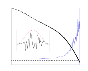
In this section, a systematic investigation of the evolution of the internal intermittency of turbulent velocity and passive-scalar fields in wavenumber space is undertaken by way of an analysis of the higher-order spectral moments of turbulent time series. To this end, figures 5 and 6 respectively plot the spectral skewness and spectral kurtosis of a turbulent velocity field at  $R_{\lambda }=582$ as a function of normalised wavenumber
  $\kappa _1 \eta$, where
  $\eta$ is the Kolmogorov length scale. Power spectra are also plotted in these figures to better identify the various ranges of the flow (e.g. the inertial subrange). Note that these results were obtained using STFT windows of length
  $N=625\eta$. Although shorter windows would have maximised the higher-order spectral moments, longer windows include a larger range of frequencies, which is preferable at the initial stages of the analysis, given that they allow low-frequency deviations from Gaussianity to be captured. Results obtained using shorter windows that highlight the intermittency at higher frequencies are presented in subsequent sections.

Figure 5. Longitudinal ( $u$) velocity spectrum (solid black line) and spectral skewness (dashed blue line) at
  $R_\lambda =582$. Results are obtained using a window length
  $625\eta$.

Figure 6. Longitudinal ( $u$) velocity spectrum (solid black line) and spectral kurtosis (dashed blue line) at
  $R_\lambda =582$. Results are obtained using a window length
  $625\eta$.
It is worthwhile noting that some insight could have been gained from calculating the higher-order moments of differences in turbulent quantities (e.g. the kurtosis of velocity increments,  $K_{\Delta u}$, (
 $\Delta u = [u(x+r)-u(x)]$)), as those are the real-space analogues of the spectral moments of equivalent statistical order. However, as noted in § 1, an important reason for undertaking the present analysis in the spectral domain is that structure functions (e.g.
  $\Delta u(r)$) include contributions from all scales less than or equal to the scale
  $r$ (see, for example, Meyer et al. Reference Meyer, Mydlarski and Danaila2018), whereas spectra quantify the contribution only at a specific scale (
 $\kappa _1 \sim 1/r$).
The first important observation to be made regarding figures 5 and 6 is that both higher-order spectral moments asymptotically tend to their Gaussian values ( $\tilde {S}=\varGamma (5/2)$ and
  $\tilde {K}=2$) at large scales (low wavenumbers), thus confirming that little intermittency is present at the largest scales of the turbulence. Conversely, at high wavenumbers, one observes a sharp increase in both the spectral skewness and kurtosis, thus highlighting the highly intermittent behaviour of the turbulent velocity field at dissipative scales. Note that these observations are consistent with figure 6 of Brun & Pumir (Reference Brun and Pumir2001) and figure 1(a) of Chevillard et al. (Reference Chevillard, Mazellier, Poulain, Gagne and Baudet2005), who observed a plateau at large scales and increased intermittent activity in the dissipation range using fourth-order spectral moments applied to time series of velocity fields from numerical and experimental data, respectively. Chevillard et al. (Reference Chevillard, Mazellier, Poulain, Gagne and Baudet2005) also calculated the fourth-order spectral moment of an intermittent synthetic signal, as a proxy for turbulence at high Reynolds number (with no dissipation range), which yielded a similar plateau. They found that the magnitude of the plateau evolved as a power law of the width of the windowing function (arguing that longer windows were associated with larger scales and therefore lower values of the fourth-order spectral moments). However, our prior analysis demonstrated that longer window lengths are associated with lower values of the higher-order spectral moments due to consequences of the central limit theorem.
These preliminary observations clearly demonstrate that both higher-order spectral moments studied herein are able to detect deviations from Gaussianity and thus internal intermittency. Moreover, the insight provided by the higher-order spectral moments compared with time-domain statistical moments is also readily demonstrated. The calculation of higher-order moments in short spectral bands allows (i) deviations from Gaussian behaviour to be located in wavenumber space, and (ii) an evaluation of the relative magnitude of the deviations from Gaussianity at each scale. The deviation from Gaussianity extends to the high-wavenumber end of the inertial subrange. This will be further discussed when short-window results are introduced, as these provide an even better depiction of inertial subrange intermittency. These features of higher-order spectral moments will be used to study the internal intermittency of turbulent velocity and passive-scalar fields in the following subsections.
4.3. Reynolds-number dependence of higher-order spectral moments
Figure 7 depicts the evolution of the spectral skewness and kurtosis of the longitudinal velocity fluctuations ( $u$), transverse velocity fluctuations (
 $v$) and scalar fluctuation (
 $\theta$) in grid-generated turbulence at five different Reynolds numbers in the range
  $35\leq R_\lambda \leq 582$. Note that these results were generated using a shorter window length of
  $N=150\eta$, thereby highlighting transient behaviour at the smaller-scale end of the inertial subrange and in the dissipation range. The results depict a very clear dependence on Reynolds number, even at
  $R_\lambda <100$ which was previously observed to be the threshold for the hydrodynamic (inertial-range) intermittency exponent (
 $\mu$) to depart from zero (Mydlarski & Warhaft Reference Mydlarski and Warhaft1998). However, Mydlarski & Warhaft (Reference Mydlarski and Warhaft1998) observed the scalar field intermittency exponent (
 $\mu _\theta$) to be non-zero at even the lowest of Reynolds/Péclet numbers. A significant increase in non-Gaussian behaviour is exhibited by all spectral moments as the Reynolds number is increased. Note that this increase in magnitude of the spectral moments occurs at all scales covered by the chosen window length, and applies to all turbulent fields under study (i.e.
  $u$,
$u$,  $v$ and
  $\theta$). Moreover, note that the scale at which a strong and rapid departure from Gaussianity is observed shifts towards larger scales as the Reynolds number increased.

Figure 7. Spectral skewness (a,c,e) and kurtosis (b,d,f) of the longitudinal velocity fluctuations  $u$ (a,b), the transverse velocity fluctuations
  $v$ (c,d) and the scalar (temperature) fluctuations
  $\theta$ (e,f) at
  $R_\lambda = 35$ (
 $\ast$, blue),
  $R_\lambda = 86$ (
 $\Diamond$, magenta),
  $R_\lambda = 140$ (
 $+$, green),
  $R_\lambda = 306$ (
 $\circ$, black) and
  $R_\lambda = 582$ (
 $\Box$, red). Results are obtained using a window length
  $N=150\eta$.
One can further explore the Reynolds-number dependence of internal intermittency by investigating the evolution of the magnitude of the higher-order spectral moments evaluated at a particular length scale. A length scale of interest is the wavenumber at which the dissipations of turbulent kinetic energy and turbulent scalar variance spectra peak, which is observed to occur around  $\kappa _1\eta = 0.2$ for the velocity and scalar fields, although the exact location of this peak is Reynolds-number dependent (Tennekes & Lumley Reference Tennekes and Lumley1972; Mydlarski & Warhaft Reference Mydlarski and Warhaft1996, Reference Mydlarski and Warhaft1998). The value of the spectral skewness and kurtosis at a normalised wavenumber of
  $\kappa _1\eta = 0.2$ is plotted in figure 8 as a function of
  $R_\lambda$ over the range
  $35\leq R_\lambda \leq 731$. Note that the higher-order spectral moments shown in figure 8 were obtained using the same window length as that used in figure 7 (
 $N=150\eta$). Although some scatter is observed, the plots confirm the increase in both the spectral skewness and spectral kurtosis (and therefore in internal intermittency) at a fixed wavenumber as
  $R_\lambda$ is increased. Moreover, considering each higher-order spectral moment individually, note that the power law fits are consistent for the longitudinal and transverse velocity and passive-scalar fields, with
  $\tilde {S} (\kappa _1\eta =0.2)$ increasing as
  $R_\lambda ^{0.1}$ and
  $\tilde {K} (\kappa _1\eta =0.2)$ increasing as
  $R_\lambda ^{0.3}$ for the spectral kurtosis. The evolution of the spectral skewness and kurtosis is further explored in figure 9, in which the Reynolds-number dependence of both spectral moments evaluated at
  $\kappa _1\eta =0.8$ is investigated. Note that the chosen length scale of
  $\kappa _1\eta =0.8$ is believed to offer a good representation of the intermittent behaviour of the flow as the Kolmogorov length scale is approached (
 $\kappa _1\eta \rightarrow 1$), while staying sufficiently far away from the Kolmogorov length scale where errors due to low-pass filter roll-off and probe frequency resolution (especially with cold-wire thermometers) may occur (Kuo & Corrsin Reference Kuo and Corrsin1971). As was the case at
  $\kappa _1\eta =0.2$, the Reynolds-number dependence of the spectral skewness and kurtosis at
  $\kappa _1\eta =0.8$ is consistent with a power law increase, although a stronger dependence on Reynolds number is observed at this smaller length scale. These changes in power law exponents with
  $\kappa _1\eta$ highlight the wavenumber dependence of the evolution of the higher-order spectral moments with
  $R_\lambda$.

Figure 8. Reynolds-number dependence of the spectral skewness (a,c,e) and kurtosis (b,d,f) of the longitudinal velocity fluctuations  $u$ (a,b), the transverse velocity fluctuations
  $v$ (c,d) and the passive-scalar (temperature) fluctuations
  $\theta$ (e,f) evaluated at
  $\kappa _1\eta =0.2$. The solid black lines represent the best fit power laws. Results are obtained using a window length
  $N=150\eta$.

Figure 9. Reynolds-number dependence of the spectral skewness (a,c,e) and kurtosis (b,d,f) of the longitudinal velocity fluctuations  $u$ (a,b), the transverse velocity fluctuations
  $v$ (c,d) and the passive-scalar (temperature) fluctuations
  $\theta$ (e,f) evaluated at
  $\kappa _1\eta =0.8$. The solid black lines represent the best fit power laws. Results are obtained using a window length
  $N=150\eta$.
To place these results in the context of prior studies of internal intermittency, it is of benefit to compare the present work with prior investigations of the dependence of internal intermittency on Reynolds number, which was historically investigated using the kurtosis of derivatives of turbulence quantities (e.g.  $K_{\partial u/\partial x}$,
  $K_{\partial \theta /\partial x}$) as measures of the degree of intermittency in turbulent flows (see Van Atta & Antonia Reference Van Atta and Antonia1980; Sreenivasan & Antonia Reference Sreenivasan and Antonia1997). Studies have shown that
  $K_{\partial u/\partial x}$ and
  $K_{\partial \theta /\partial x}$ are strongly dependent on Reynolds number, with
  $K_{\partial u/\partial x}$ increasing as
  $\sim R_\lambda ^{3/8}$ (Van Atta & Antonia Reference Van Atta and Antonia1980), which is consistent with the observations of the spectral kurtosis evaluated at
  $\kappa _1\eta =0.2$ (figure 8). As previously noted, the Reynolds-number dependence of the spectral skewness and kurtosis was specifically evaluated at
  $\kappa _1\eta =0.2$ because this normalised wavenumber (
 $\kappa _1\eta =0.2$) approximately corresponds to that of the peak of the dissipation spectrum (Tennekes & Lumley Reference Tennekes and Lumley1972). Given that dissipation spectra can also be interpreted as the spectra of the derivative, studying the higher-order spectral moments at
  $\kappa _1\eta =0.2$ evaluates them at the wavenumber at which the derivative has its maximum contribution, thus explaining the agreement between the observed trends (
 $\sim R_\lambda ^{0.3}$) and those obtained by examining the Reynolds-number dependencies of
  $K_{\partial u/\partial x}$ and
  $K_{\partial \theta /\partial x}$ (
 $\sim R_\lambda ^{3/8}$). However, it bears reiterating that the present results have demonstrated that the Reynolds-number dependence of internal intermittency depends upon wavenumber, as demonstrated by the scale-by-scale analysis achieved by way of higher-order spectral moments.
In addition to the above results, another approach was also employed in an attempt to investigate any possible Reynolds-number dependencies associated with the use of a window length of fixed multiples of  $\eta$ as the Reynolds number changes. To this end, the data were reanalysed using a window length (
 $N$) that evolved with Reynolds number in such a way the window length was equal to the separation that corresponds to the mid-point of the inertial subrange for each flow. To determine the required window length for this approach, we followed the methodology employed in Mydlarski & Warhaft (Reference Mydlarski and Warhaft1996, Reference Mydlarski and Warhaft1998), who developed an approach for the calculation of conditional statistics of inertial-range velocity and scalar increments (e.g.
  $\Delta u(r)$) as the Reynolds/Péclet number increased. This approach is depicted in figure 23 of Mydlarski & Warhaft (Reference Mydlarski and Warhaft1996). These authors chose a single value of
  $r$ (denoted as
  $r_a$ in Mydlarski & Warhaft Reference Mydlarski and Warhaft1996) that corresponded to the wavenumber
  $\kappa _1$ (
 $r = 2{\rm \pi} /\kappa _1$) that lay half-way between the beginning and end of the scaling range for each spectrum. Thus as the scaling range dilated with Reynolds number,
  $r_a$, remained in the same relative position within the inertial subrange. Using this approach, the window lengths varied from one case to the next, but always remained in the same relative position on the spectrum, independent of Reynolds number.
Figure 10 plots the spectral skewness and kurtosis of the  $u$,
$u$,  $v$ and
  $\theta$ fields using this approach for different Reynolds numbers for window lengths
  $N$ equal to
  $r_a$. Although there are differences in the results when this new methodology is employed to specify the window widths, the overall (quantitative and qualitative) results and trends in figures 7 and 10 remain quite similar, thus justifying the robustness of the analysis herein and confirming the relative insensitivity of the effect of window width when the Reynolds number is varied.

Figure 10. Spectral skewness (a,c,e) and kurtosis (b,d,f) of the longitudinal velocity fluctuations  $u$ (a,b), the transverse velocity fluctuations
  $v$ (c,d) and the scalar (temperature) fluctuations
  $\theta$ (e,f) at
  $R_\lambda = 35$ (
 $\ast$, blue),
  $R_\lambda = 86$ (
 $\Diamond$, magenta),
  $R_\lambda = 140$ (
 $+$, green),
  $R_\lambda = 306$ (
 $\circ$, black) and
  $R_\lambda = 582$ (
 $\Box$, red). Results are obtained using window lengths corresponding to the midpoint of the inertial subrange.
4.4. Higher-order spectral moments of turbulent scalar fields
Given the different nature of scalar fields (Pumir et al. Reference Pumir, Shraiman and Siggia1991; Holzer & Siggia Reference Holzer and Siggia1994; Warhaft Reference Warhaft2000), it is of particular interest to study the relative levels of intermittency of both velocity and passive-scalar fields. To this end, a preliminary analysis (not shown) concluded that a window length of  $N=220\eta$ captured the signal transients while also fully capturing frequencies in the dissipation range and most of the inertial–convective subrange.
Plots of the spectral skewness and kurtosis of  $u$,
$u$,  $v$ and
  $\theta$ are given in figures 11 and 12, respectively. The overall behaviour of all higher-order spectral moments is similar for all three quantities. More specifically, the curves all show a significant departure from Gaussian behaviour at small scales, and both the spectral skewness and kurtosis exhibit a higher degree of internal intermittency in the inertial–convective subrange for passive-scalar fields (compared with the longitudinal and transverse velocity fields, which are both very similar in magnitude in the inertial subrange). Note that these results are consistent with those of Mydlarski & Warhaft (Reference Mydlarski and Warhaft1998), who used the velocity and scalar intermittency exponent to show that scalar fields were more intermittent in the inertial subrange and that their level of intermittent activity increased with Reynolds number. Moreover, they also showed that the level of inertial range intermittency of passive-scalar fields remains higher than that of velocity fields at all Reynolds numbers.

Figure 11. Spectral skewness of the longitudinal velocity fluctuations  $u$ (
$u$ ( $\circ$, black), transverse velocity fluctuations
  $v$ (
$v$ ( $\Box$, blue) and scalar (temperature) fluctuations
  $\theta$ (
 $\triangle$, red) at (a)
  $R_\lambda = 85$, (b)
  $R_\lambda = 140$, (c)
  $R_\lambda = 306$ and (d)
  $R_\lambda = 582$. Results are obtained using a window length
  $N=220\eta$.

Figure 12. Spectral kurtosis of the longitudinal velocity fluctuations  $u$ (
$u$ ( $\circ$, black), transverse velocity fluctuations
  $v$ (
$v$ ( $\Box$, blue) and scalar (temperature) fluctuations
  $\theta$ (
 $\triangle$, red) at (a)
  $R_\lambda = 85$, (b)
  $R_\lambda = 140$, (c)
  $R_\lambda = 306$ and (d)
  $R_\lambda = 582$. Results are obtained using a window length
  $N=220\eta$.
The results presented in figures 11 and 12 show that the spectral skewness and spectral kurtosis of the scalar fluctuations remain at a higher level at small scales (high wavenumbers) when compared with the longitudinal and transverse velocity statistics for the two lower  $R_\lambda$ cases shown in figures 11 and 12. However, the spectral skewness and spectral kurtosis of the longitudinal and transverse velocity fluctuations undergo a rapid increase in the dissipation range and reach levels similar to that of the passive-scalar field as
  $\kappa _1\eta \rightarrow 1$ for the two higher
  $R_\lambda$ cases. This suggests that passive-scalar fields are more intermittent in the inertial–convective subrange and in part of the dissipation range, but the degree of intermittency of the streamwise and transverse velocity fields becomes similar to that of the scalar field as the Kolmogorov length scale is approached at high Reynolds numbers. This is consistent with the remarks made in § 4.3 regarding the wavenumber dependence of the Reynolds-number evolution of higher-order spectral moments. The plots of figure 9 showed that dependence of higher-order spectral moments on Reynolds number was stronger for the velocity field than the passive-scalar field at high wavenumbers. This is the reason figures 11 and 12 show that the higher-order spectral moments of both components of the velocity field reach levels similar to those of the passive-scalar field at high wavenumbers for the two highest
  $R_\lambda$ cases.
5. Summary and conclusions
Higher-order spectral moments have been used to investigate internal intermittency in grid-generated turbulent velocity and passive scalar fields. In this study, an overview of the theory behind the third- and fourth-order spectral moments was first presented. Then, a STFT-based estimator was used to develop an algorithm capable of calculating higher-order spectral moments. The estimator was validated using Gaussian and non-Gaussian test signals, and the dependence of the estimator on window length was investigated. It was demonstrated that higher-order spectral moments can be used to situate intermittency in wavenumber space and compare the relative levels of intermittency at different scales. Higher-order spectral moments of turbulent flows were shown to exhibit repeatable behaviours, asymptotically moving to Gaussian values at large scales and departing from Gaussian behaviour in the inertial subrange, reaching their maximum values at the smallest scales of the dissipation range. Additionally, it was demonstrated that higher-order spectral moments are Reynolds-number dependent. The spectral kurtoses of the longitudinal and transverse velocity fields at  $\kappa _1\eta = 0.2$ were found to increase as
  $\tilde {K}_{u_\alpha }(\kappa _1\eta =0.2)\sim R_\lambda ^{0.3}$ over the range of Reynolds numbers studied herein, which is consistent with the behaviour of the overall kurtosis of velocity derivatives observed by Van Atta & Antonia (Reference Van Atta and Antonia1980). Moreover, the Reynolds-number dependence of the intensity of internal intermittency was shown to depend on wavenumber by way of the present approach.
The magnitude and wavenumber dependence of the internal intermittency of passive-scalar fields was compared with that of velocity fields with the spectral skewness and kurtosis revealing that the level of intermittency of passive-scalar fluctuations is higher in the inertial subrange and part of the dissipation range when compared with those of the longitudinal and transverse velocity fluctuations. However, for the higher  $R_\lambda$ cases and as
  $\kappa _1\eta \rightarrow 1$, the levels of intermittency of the longitudinal and transverse velocity fluctuations were seen to increase and eventually become similar to those of the passive-scalar field.
The results herein suggest that our knowledge of internal intermittency can be expanded by way of higher-order spectral moments. In the present work, the latter provided an insightful means of investigating the Reynolds-number dependence of intermittency and comparing the intermittent behaviour of velocity and passive-scalar fields. Future work shall be aimed at comparing the wavenumber dependence and levels of intermittency between different classes of flows. It is hoped that higher-order spectral moments can be used to investigate additional turbulence phenomena, such as the evolution of the coherent structures in wall-bounded flows, or other intermittent phenomena.
Acknowledgements
The authors acknowledge the reviewers for their constructive comments, which improved this work.
Funding
Support for this work was graciously provided by the Natural Sciences and Engineering Council of Canada (Grant number RGPIN-2018-05848), as well as the United States Department of Energy (Basic Energy Sciences). The experiments were undertaken at Cornell University. Funding for S.L. was provided by the Natural Sciences and Engineering Council of Canada (Canada Graduate Scholarships – Master's program) and the Fonds de recherche du Québec – Nature et technologies (Master's research scholarships).
Declaration of interests
The authors report no conflict of interest.


