


1 Introduction
Pathways of energy dissipation in internal waves generated by tides and winds are an important piece in the puzzle of understanding vertical mixing and the global energy budget in the ocean (Munk & Wunsch Reference Munk and Wunsch1998). In this paper, we study a nonlinear mechanism of superharmonic wave generation as a result of interaction between various vertical modes of internal waves at a fixed frequency.
Linear internal wave fields in the finite-depth ocean are conveniently represented using vertical modes, which ensures that the boundary conditions on the ocean floor and the free surface (often modelled as a rigid lid) are satisfied (Gill Reference Gill1982). Internal tide generation arising from barotropic tidal flow over bottom topography is understood to result in a range of vertical modes at the semidiurnal frequency, with the high modes getting dissipated near the generation sites and the low modes travelling far (Garrett & Kunze Reference Garrett and Kunze2007). Subsequent processes such as scattering by short or tall deep ocean topography and continental shelves further transfer energy from the far-travelling low modes to higher modes at the same frequency (Johnston, Merrifield & Holloway Reference Johnston, Merrifield and Holloway2003; Klymak et al. Reference Klymak, Alford, Pinkel, Lien, Yang and Tang2011; Mathur, Carter & Peacock Reference Mathur, Carter and Peacock2014). Similarly, the spatially compact near-inertial currents excited in the mixed layer by surface winds generate a whole range of high modes, with a modal representation and the calculation of the evolution of the modal amplitudes providing insight into the mechanisms by which near-inertial waves propagate into the deep ocean (D’Asaro Reference D’Asaro1989; Balmforth & Young Reference Balmforth and Young1999). While the transfer of energy to higher modes, and hence shorter spatial scales, is generally recognized as conducive to instabilities and mixing, the exact mechanisms leading to internal wave energy dissipation are not well understood. The nonlinear effects that may result from the presence of a range of vertical modes at a given frequency in a non-uniform stratification are the focus of the current study.
One of the well-known instability mechanisms in internal waves is the resonant triad interaction (RTI) (Staquet & Sommeria Reference Staquet and Sommeria2002). In uniformly stratified fluid of infinite horizontal and vertical extents, three interacting internal waves satisfying the relations
 $\unicode[STIX]{x1D714}_{1}+\unicode[STIX]{x1D714}_{2}+\unicode[STIX]{x1D714}_{3}=0$
and
$\unicode[STIX]{x1D714}_{1}+\unicode[STIX]{x1D714}_{2}+\unicode[STIX]{x1D714}_{3}=0$
and
 $\boldsymbol{k}_{1}+\boldsymbol{k}_{2}+\boldsymbol{k}_{3}=0$
form a resonant triad, where
$\boldsymbol{k}_{1}+\boldsymbol{k}_{2}+\boldsymbol{k}_{3}=0$
form a resonant triad, where
 $\boldsymbol{k}_{1,2,3}$
are the wave vectors and
$\boldsymbol{k}_{1,2,3}$
are the wave vectors and
 $\unicode[STIX]{x1D714}_{1,2,3}$
are the corresponding frequencies (positive or negative) obtained from the linear internal wave dispersion relation (Hasselmann Reference Hasselmann1967; LeBlond & Mysak Reference LeBlond and Mysak1981). In arbitrary non-uniform stratifications, however, there exists no such simple analytical criterion for a pure resonant wave triad. In this paper, we show that pure resonant triads exist in a finite-depth non-uniform stratification, and we also identify the conditions for the same.
$\unicode[STIX]{x1D714}_{1,2,3}$
are the corresponding frequencies (positive or negative) obtained from the linear internal wave dispersion relation (Hasselmann Reference Hasselmann1967; LeBlond & Mysak Reference LeBlond and Mysak1981). In arbitrary non-uniform stratifications, however, there exists no such simple analytical criterion for a pure resonant wave triad. In this paper, we show that pure resonant triads exist in a finite-depth non-uniform stratification, and we also identify the conditions for the same.
An important consequence of RTI is the parametric subharmonic instability (PSI), where a primary plane internal wave (above a threshold amplitude) at frequency
 $\unicode[STIX]{x1D714}_{0}$
in a viscous, uniformly stratified fluid results in the growth of secondary waves that form a resonant triad with the primary wave (Koudella & Staquet Reference Koudella and Staquet2006; Bourget et al.
Reference Bourget, Dauxois, Joubaud and Odier2013). The secondary waves with the maximum growth rate occur at frequencies
$\unicode[STIX]{x1D714}_{0}$
in a viscous, uniformly stratified fluid results in the growth of secondary waves that form a resonant triad with the primary wave (Koudella & Staquet Reference Koudella and Staquet2006; Bourget et al.
Reference Bourget, Dauxois, Joubaud and Odier2013). The secondary waves with the maximum growth rate occur at frequencies
 $\unicode[STIX]{x1D714}_{1,2}<\unicode[STIX]{x1D714}_{0}$
, with the relation
$\unicode[STIX]{x1D714}_{1,2}<\unicode[STIX]{x1D714}_{0}$
, with the relation
 $\unicode[STIX]{x1D714}_{1}\approx \unicode[STIX]{x1D714}_{2}\approx \unicode[STIX]{x1D714}_{0}/2$
holding in the limit of relatively large wavenumbers of the secondary waves (Staquet & Sommeria Reference Staquet and Sommeria2002). In an internal wave beam, constructed as a superposition of unidirectional plane waves at a fixed frequency, PSI is less likely to occur, with various studies highlighting the importance of incorporating the effect of the finite spatial extent of the wave beam (Clark & Sutherland Reference Clark and Sutherland2010; Bourget et al.
Reference Bourget, Dauxois, Joubaud and Odier2013; Karimi & Akylas Reference Karimi and Akylas2014). PSI has been observed in experimental studies of propagating internal wave modes too, with the triads corresponding to large theoretical growth rates shown to emerge (Martin, Simmons & Wunsch Reference Martin, Simmons and Wunsch1972; Joubaud et al.
Reference Joubaud, Munroe, Odier and Dauxois2012).
$\unicode[STIX]{x1D714}_{1}\approx \unicode[STIX]{x1D714}_{2}\approx \unicode[STIX]{x1D714}_{0}/2$
holding in the limit of relatively large wavenumbers of the secondary waves (Staquet & Sommeria Reference Staquet and Sommeria2002). In an internal wave beam, constructed as a superposition of unidirectional plane waves at a fixed frequency, PSI is less likely to occur, with various studies highlighting the importance of incorporating the effect of the finite spatial extent of the wave beam (Clark & Sutherland Reference Clark and Sutherland2010; Bourget et al.
Reference Bourget, Dauxois, Joubaud and Odier2013; Karimi & Akylas Reference Karimi and Akylas2014). PSI has been observed in experimental studies of propagating internal wave modes too, with the triads corresponding to large theoretical growth rates shown to emerge (Martin, Simmons & Wunsch Reference Martin, Simmons and Wunsch1972; Joubaud et al.
Reference Joubaud, Munroe, Odier and Dauxois2012).
RTI can also result from the presence of two finite-amplitude primary waves. For example, interaction between reflecting or colliding wave beams at a fixed frequency
 $\unicode[STIX]{x1D714}$
results in the generation of higher harmonic wave beams at frequency
$\unicode[STIX]{x1D714}$
results in the generation of higher harmonic wave beams at frequency
 $2\unicode[STIX]{x1D714}$
(Peacock & Tabaei Reference Peacock and Tabaei2005; Tabaei, Akylas & Lamb Reference Tabaei, Akylas and Lamb2005). The interaction between plane waves contained within a unidirectional wave beam at frequency
$2\unicode[STIX]{x1D714}$
(Peacock & Tabaei Reference Peacock and Tabaei2005; Tabaei, Akylas & Lamb Reference Tabaei, Akylas and Lamb2005). The interaction between plane waves contained within a unidirectional wave beam at frequency
 $\unicode[STIX]{x1D714}$
, however, does not result in the generation of higher harmonics, as the unidirectional wave beam in a uniformly stratified fluid of an infinite extent is an exact solution of the nonlinear equations as well (Tabaei & Akylas Reference Tabaei and Akylas2003). In contrast, in a finite-depth fluid, any linear internal wave field is a superposition of modes, and hence not necessarily an exact solution to the nonlinear equations of motion. As shown by Thorpe (Reference Thorpe1966) for a uniform stratification with no background rotation, two primary internal wave modes at a fixed frequency can interact to form a resonant triad.
$\unicode[STIX]{x1D714}$
, however, does not result in the generation of higher harmonics, as the unidirectional wave beam in a uniformly stratified fluid of an infinite extent is an exact solution of the nonlinear equations as well (Tabaei & Akylas Reference Tabaei and Akylas2003). In contrast, in a finite-depth fluid, any linear internal wave field is a superposition of modes, and hence not necessarily an exact solution to the nonlinear equations of motion. As shown by Thorpe (Reference Thorpe1966) for a uniform stratification with no background rotation, two primary internal wave modes at a fixed frequency can interact to form a resonant triad.
To the best of our knowledge, while the generation of subharmonic and superharmonic waves in non-uniform stratifications has been reported in field observations (Xie et al. Reference Xie, Shang, Haren and Chen2013), theoretical studies (Thorpe Reference Thorpe1998; Young, Tsang & Balmforth Reference Young, Tsang and Balmforth2008; Wunsch Reference Wunsch2015), laboratory experiments (Wunsch & Brandt Reference Wunsch and Brandt2012; Wunsch et al. Reference Wunsch, Delwiche, Frederick and Brandt2015; Ghaemsaidi et al. Reference Ghaemsaidi, Joubaud, Dauxois, Odier and Peacock2016) and numerical simulations (Gayen & Sarkar Reference Gayen and Sarkar2013; Diamessis et al. Reference Diamessis, Wunsch, Delwiche and Richter2014; Wunsch et al. Reference Wunsch, Ku, Delwiche and Awadallah2014), no previous studies have rigorously defined and identified resonant triads arising from modal interactions in non-uniformly stratified finite-depth media. In this paper, we construct the steady-state weakly nonlinear solution that corresponds to the leading-order solution containing an arbitrary sum of vertical modes at a given frequency in non-uniformly stratified media with background rotation, and thereby identify resonant triads via the divergence of the weakly nonlinear solution. Section 2 discusses the theory, followed by the results in § 3. The relevance of our theoretical results to two different oceanic scenarios is presented in § 4, followed by the conclusions in § 5.
2 Theory
The nonlinear governing equations for two-dimensional, incompressible, inviscid internal waves on the
 $f$
-plane under the Boussinesq approximation are (LeBlond & Mysak Reference LeBlond and Mysak1981)
$f$
-plane under the Boussinesq approximation are (LeBlond & Mysak Reference LeBlond and Mysak1981)
 $$\begin{eqnarray}\displaystyle & \displaystyle {\displaystyle \frac{\unicode[STIX]{x2202}^{2}}{\unicode[STIX]{x2202}t^{2}}}(\unicode[STIX]{x1D6FB}^{2}\unicode[STIX]{x1D713})+f^{2}{\displaystyle \frac{\unicode[STIX]{x2202}^{2}\unicode[STIX]{x1D713}}{\unicode[STIX]{x2202}z^{2}}}={\displaystyle \frac{g}{\unicode[STIX]{x1D70C}^{\ast }}}{\displaystyle \frac{\unicode[STIX]{x2202}}{\unicode[STIX]{x2202}x}}[J(\unicode[STIX]{x1D713},\unicode[STIX]{x1D70C})]-{\displaystyle \frac{\unicode[STIX]{x2202}}{\unicode[STIX]{x2202}t}}[J(\unicode[STIX]{x1D713},\unicode[STIX]{x1D6FB}^{2}\unicode[STIX]{x1D713})]+f{\displaystyle \frac{\unicode[STIX]{x2202}}{\unicode[STIX]{x2202}z}}[J(\unicode[STIX]{x1D713},v)], & \displaystyle\end{eqnarray}$$
 $$\begin{eqnarray}\displaystyle & \displaystyle {\displaystyle \frac{\unicode[STIX]{x2202}\unicode[STIX]{x1D70C}}{\unicode[STIX]{x2202}t}}=-J(\unicode[STIX]{x1D713},\unicode[STIX]{x1D70C}), & \displaystyle\end{eqnarray}$$
 $$\begin{eqnarray}\displaystyle & \displaystyle {\displaystyle \frac{\unicode[STIX]{x2202}v}{\unicode[STIX]{x2202}t}}+J(\unicode[STIX]{x1D713},v)=f{\displaystyle \frac{\unicode[STIX]{x2202}\unicode[STIX]{x1D713}}{\unicode[STIX]{x2202}z}}, & \displaystyle\end{eqnarray}$$
where
 $x$
and
$x$
and
 $z$
are the horizontal and vertical coordinates and
$z$
are the horizontal and vertical coordinates and
 $t$
is time;
$t$
is time;
 $\unicode[STIX]{x1D713}(x,z,t)$
,
$\unicode[STIX]{x1D713}(x,z,t)$
,
 $v(x,z,t)$
and
$v(x,z,t)$
and
 $\unicode[STIX]{x1D70C}(x,z,t)$
are the streamfunction,
$\unicode[STIX]{x1D70C}(x,z,t)$
are the streamfunction,
 $y$
-component of velocity and density, respectively, with the velocity components in the
$y$
-component of velocity and density, respectively, with the velocity components in the
 $(x,z)$
plane given by
$(x,z)$
plane given by
 $(u,w)=(-\unicode[STIX]{x2202}\unicode[STIX]{x1D713}/\unicode[STIX]{x2202}z,\unicode[STIX]{x2202}\unicode[STIX]{x1D713}/\unicode[STIX]{x2202}x)$
;
$(u,w)=(-\unicode[STIX]{x2202}\unicode[STIX]{x1D713}/\unicode[STIX]{x2202}z,\unicode[STIX]{x2202}\unicode[STIX]{x1D713}/\unicode[STIX]{x2202}x)$
;
 $\unicode[STIX]{x1D70C}^{\ast }$
is a reference constant density,
$\unicode[STIX]{x1D70C}^{\ast }$
is a reference constant density,
 $f$
the Coriolis frequency and
$f$
the Coriolis frequency and
 $g$
the acceleration due to gravity. The Jacobian operator
$g$
the acceleration due to gravity. The Jacobian operator
 $J$
is defined as
$J$
is defined as
 $J(A,B)=(\unicode[STIX]{x2202}A/\unicode[STIX]{x2202}x)(\unicode[STIX]{x2202}B/\unicode[STIX]{x2202}z)-(\unicode[STIX]{x2202}B/\unicode[STIX]{x2202}x)(\unicode[STIX]{x2202}A/\unicode[STIX]{x2202}z)$
, and
$J(A,B)=(\unicode[STIX]{x2202}A/\unicode[STIX]{x2202}x)(\unicode[STIX]{x2202}B/\unicode[STIX]{x2202}z)-(\unicode[STIX]{x2202}B/\unicode[STIX]{x2202}x)(\unicode[STIX]{x2202}A/\unicode[STIX]{x2202}z)$
, and
 $\unicode[STIX]{x1D6FB}^{2}=\unicode[STIX]{x2202}^{2}/\unicode[STIX]{x2202}x^{2}+\unicode[STIX]{x2202}^{2}/\unicode[STIX]{x2202}z^{2}$
. A no-normal-flow boundary condition at the horizontal boundaries of the fluid of depth
$\unicode[STIX]{x1D6FB}^{2}=\unicode[STIX]{x2202}^{2}/\unicode[STIX]{x2202}x^{2}+\unicode[STIX]{x2202}^{2}/\unicode[STIX]{x2202}z^{2}$
. A no-normal-flow boundary condition at the horizontal boundaries of the fluid of depth
 $H$
is specified as
$H$
is specified as
 $\unicode[STIX]{x1D713}(x,z=0,t)=\unicode[STIX]{x1D713}(x,z=H,t)=0$
. We now proceed to perform a weakly nonlinear analysis, which is a well-established mathematical tool as is described in LeBlond & Mysak (Reference LeBlond and Mysak1981).
$\unicode[STIX]{x1D713}(x,z=0,t)=\unicode[STIX]{x1D713}(x,z=H,t)=0$
. We now proceed to perform a weakly nonlinear analysis, which is a well-established mathematical tool as is described in LeBlond & Mysak (Reference LeBlond and Mysak1981).
In the framework of regular perturbation expansion, we seek solutions of the form
 $$\begin{eqnarray}(\unicode[STIX]{x1D713},v,\unicode[STIX]{x1D70C})=(\unicode[STIX]{x1D713}_{0},v_{0},\unicode[STIX]{x1D70C}_{0})+\unicode[STIX]{x1D716}(\unicode[STIX]{x1D713}_{1},v_{1},\unicode[STIX]{x1D70C}_{1})+\unicode[STIX]{x1D716}^{2}(\unicode[STIX]{x1D713}_{2},v_{2},\unicode[STIX]{x1D70C}_{2})+\cdots \,,\end{eqnarray}$$
where the small parameter
 $\unicode[STIX]{x1D716}$
quantifies the relative magnitude of the nonlinear terms in the governing equations. Substituting the solution forms of
$\unicode[STIX]{x1D716}$
quantifies the relative magnitude of the nonlinear terms in the governing equations. Substituting the solution forms of
 $(\unicode[STIX]{x1D713},v,\unicode[STIX]{x1D70C})$
in (2.4) into (2.1)–(2.3), we obtain
$(\unicode[STIX]{x1D713},v,\unicode[STIX]{x1D70C})$
in (2.4) into (2.1)–(2.3), we obtain
 $$\begin{eqnarray}\displaystyle & & \displaystyle \left[{\displaystyle \frac{\unicode[STIX]{x2202}^{2}}{\unicode[STIX]{x2202}t^{2}}}(\unicode[STIX]{x1D6FB}^{2}\unicode[STIX]{x1D713}_{0})+f^{2}{\displaystyle \frac{\unicode[STIX]{x2202}^{2}\unicode[STIX]{x1D713}_{0}}{\unicode[STIX]{x2202}z^{2}}}\right]+\unicode[STIX]{x1D716}\left[{\displaystyle \frac{\unicode[STIX]{x2202}^{2}}{\unicode[STIX]{x2202}t^{2}}}(\unicode[STIX]{x1D6FB}^{2}\unicode[STIX]{x1D713}_{1})+f^{2}{\displaystyle \frac{\unicode[STIX]{x2202}^{2}\unicode[STIX]{x1D713}_{1}}{\unicode[STIX]{x2202}z^{2}}}\right]+\unicode[STIX]{x1D716}^{2}\left[{\displaystyle \frac{\unicode[STIX]{x2202}^{2}}{\unicode[STIX]{x2202}t^{2}}}(\unicode[STIX]{x1D6FB}^{2}\unicode[STIX]{x1D713}_{2})+f^{2}{\displaystyle \frac{\unicode[STIX]{x2202}^{2}\unicode[STIX]{x1D713}_{2}}{\unicode[STIX]{x2202}z^{2}}}\right]\nonumber\\ \displaystyle & & \displaystyle \quad =\left[{\displaystyle \frac{g}{\unicode[STIX]{x1D70C}^{\ast }}}{\displaystyle \frac{\unicode[STIX]{x2202}}{\unicode[STIX]{x2202}x}}[J(\unicode[STIX]{x1D713}_{0},\unicode[STIX]{x1D70C}_{0})]-{\displaystyle \frac{\unicode[STIX]{x2202}}{\unicode[STIX]{x2202}t}}[J(\unicode[STIX]{x1D713}_{0},\unicode[STIX]{x1D6FB}^{2}\unicode[STIX]{x1D713}_{0})]+f{\displaystyle \frac{\unicode[STIX]{x2202}}{\unicode[STIX]{x2202}z}}(J(\unicode[STIX]{x1D713}_{0},v_{0}))\right]\nonumber\\ \displaystyle & & \displaystyle \qquad +\,\unicode[STIX]{x1D716}\left[{\displaystyle \frac{g}{\unicode[STIX]{x1D70C}^{\ast }}}{\displaystyle \frac{\unicode[STIX]{x2202}}{\unicode[STIX]{x2202}x}}[J(\unicode[STIX]{x1D713}_{0},\unicode[STIX]{x1D70C}_{1})+J(\unicode[STIX]{x1D713}_{1},\unicode[STIX]{x1D70C}_{0})]-{\displaystyle \frac{\unicode[STIX]{x2202}}{\unicode[STIX]{x2202}t}}[J(\unicode[STIX]{x1D713}_{0},\unicode[STIX]{x1D6FB}^{2}\unicode[STIX]{x1D713}_{1})+J(\unicode[STIX]{x1D713}_{1},\unicode[STIX]{x1D6FB}^{2}\unicode[STIX]{x1D713}_{0})]\right.\nonumber\\ \displaystyle & & \displaystyle \qquad \left.+\,\,f{\displaystyle \frac{\unicode[STIX]{x2202}}{\unicode[STIX]{x2202}z}}[J(\unicode[STIX]{x1D713}_{0},v_{1})+J(\unicode[STIX]{x1D713}_{1},v_{0})]\right]+\unicode[STIX]{x1D716}^{2}\left[{\displaystyle \frac{g}{\unicode[STIX]{x1D70C}^{\ast }}}{\displaystyle \frac{\unicode[STIX]{x2202}}{\unicode[STIX]{x2202}x}}[J(\unicode[STIX]{x1D713}_{0},\unicode[STIX]{x1D70C}_{2})+J(\unicode[STIX]{x1D713}_{1},\unicode[STIX]{x1D70C}_{1})+J(\unicode[STIX]{x1D713}_{2},\unicode[STIX]{x1D70C}_{0})]\right.\nonumber\\ \displaystyle & & \displaystyle \qquad -\,{\displaystyle \frac{\unicode[STIX]{x2202}}{\unicode[STIX]{x2202}t}}[J(\unicode[STIX]{x1D713}_{0},\unicode[STIX]{x1D6FB}^{2}\unicode[STIX]{x1D713}_{2})+J(\unicode[STIX]{x1D713}_{1},\unicode[STIX]{x1D6FB}^{2}\unicode[STIX]{x1D713}_{1})+J(\unicode[STIX]{x1D713}_{2},\unicode[STIX]{x1D6FB}^{2}\unicode[STIX]{x1D713}_{0})]\nonumber\\ \displaystyle & & \displaystyle \qquad +\,\,f\left.{\displaystyle \frac{\unicode[STIX]{x2202}}{\unicode[STIX]{x2202}z}}[J(\unicode[STIX]{x1D713}_{0},v_{2})+J(\unicode[STIX]{x1D713}_{1},v_{1})+J(\unicode[STIX]{x1D713}_{2},v_{0})]\right]\end{eqnarray}$$
 $$\begin{eqnarray}\displaystyle & & \displaystyle {\displaystyle \frac{\unicode[STIX]{x2202}\unicode[STIX]{x1D70C}_{0}}{\unicode[STIX]{x2202}t}}+\unicode[STIX]{x1D716}\left[{\displaystyle \frac{\unicode[STIX]{x2202}\unicode[STIX]{x1D70C}_{1}}{\unicode[STIX]{x2202}t}}\right]+\unicode[STIX]{x1D716}^{2}\left[{\displaystyle \frac{\unicode[STIX]{x2202}\unicode[STIX]{x1D70C}_{2}}{\unicode[STIX]{x2202}t}}\right]=-J(\unicode[STIX]{x1D713}_{0},\unicode[STIX]{x1D70C}_{0})-\unicode[STIX]{x1D716}[J(\unicode[STIX]{x1D713}_{0},\unicode[STIX]{x1D70C}_{1})+J(\unicode[STIX]{x1D713}_{1},\unicode[STIX]{x1D70C}_{0})]\nonumber\\ \displaystyle & & \displaystyle \qquad -\,\unicode[STIX]{x1D716}^{2}[J(\unicode[STIX]{x1D713}_{0},\unicode[STIX]{x1D70C}_{2})+J(\unicode[STIX]{x1D713}_{1},\unicode[STIX]{x1D70C}_{1})+J(\unicode[STIX]{x1D713}_{2},\unicode[STIX]{x1D70C}_{0})],\end{eqnarray}$$
 $$\begin{eqnarray}\displaystyle & & \displaystyle {\displaystyle \frac{\unicode[STIX]{x2202}v_{0}}{\unicode[STIX]{x2202}t}}+J(\unicode[STIX]{x1D713}_{0},v_{0})+\unicode[STIX]{x1D716}\left[{\displaystyle \frac{\unicode[STIX]{x2202}v_{1}}{\unicode[STIX]{x2202}t}}+J(\unicode[STIX]{x1D713}_{0},v_{1})+J(\unicode[STIX]{x1D713}_{1},v_{0})\right]\nonumber\\ \displaystyle & & \displaystyle \qquad +\,\unicode[STIX]{x1D716}^{2}\left[{\displaystyle \frac{\unicode[STIX]{x2202}v_{2}}{\unicode[STIX]{x2202}t}}+J(\unicode[STIX]{x1D713}_{0},v_{2})+J(\unicode[STIX]{x1D713}_{1},v_{1})+J(\unicode[STIX]{x1D713}_{2},v_{0})\right]\nonumber\\ \displaystyle & & \displaystyle \quad =\,f{\displaystyle \frac{\unicode[STIX]{x2202}\unicode[STIX]{x1D713}_{0}}{\unicode[STIX]{x2202}z}}+\unicode[STIX]{x1D716}f{\displaystyle \frac{\unicode[STIX]{x2202}\unicode[STIX]{x1D713}_{1}}{\unicode[STIX]{x2202}z}}+\unicode[STIX]{x1D716}^{2}f{\displaystyle \frac{\unicode[STIX]{x2202}\unicode[STIX]{x1D713}_{2}}{\unicode[STIX]{x2202}z}}.\end{eqnarray}$$
The solution at
 $\mathit{O}(\unicode[STIX]{x1D716}^{0})$
is assumed as
$\mathit{O}(\unicode[STIX]{x1D716}^{0})$
is assumed as
 $\unicode[STIX]{x1D713}_{0}=0$
,
$\unicode[STIX]{x1D713}_{0}=0$
,
 $v_{0}=0$
and
$v_{0}=0$
and
 $\unicode[STIX]{x1D70C}_{0}=\bar{\unicode[STIX]{x1D70C}}(z)$
with the stratification profile
$\unicode[STIX]{x1D70C}_{0}=\bar{\unicode[STIX]{x1D70C}}(z)$
with the stratification profile
 $N(z)=\sqrt{(-g/\unicode[STIX]{x1D70C}^{\ast })\,\text{d}\bar{\unicode[STIX]{x1D70C}}/\text{d}z}$
. In other words, the background flow is described by a static, stably stratified fluid.
$N(z)=\sqrt{(-g/\unicode[STIX]{x1D70C}^{\ast })\,\text{d}\bar{\unicode[STIX]{x1D70C}}/\text{d}z}$
. In other words, the background flow is described by a static, stably stratified fluid.
Substituting
 $(\unicode[STIX]{x1D713}_{0},\unicode[STIX]{x1D70C}_{0},v_{0})$
into (2.5)–(2.7) and retaining only the
$(\unicode[STIX]{x1D713}_{0},\unicode[STIX]{x1D70C}_{0},v_{0})$
into (2.5)–(2.7) and retaining only the
 $\mathit{O}(\unicode[STIX]{x1D716})$
terms, we obtain the governing equations for
$\mathit{O}(\unicode[STIX]{x1D716})$
terms, we obtain the governing equations for
 $(\unicode[STIX]{x1D713}_{1},\unicode[STIX]{x1D70C}_{1},v_{1})$
as
$(\unicode[STIX]{x1D713}_{1},\unicode[STIX]{x1D70C}_{1},v_{1})$
as
 $$\begin{eqnarray}\displaystyle & \displaystyle {\displaystyle \frac{\unicode[STIX]{x2202}^{2}}{\unicode[STIX]{x2202}t^{2}}}(\unicode[STIX]{x1D6FB}^{2}\unicode[STIX]{x1D713}_{1})+f^{2}{\displaystyle \frac{\unicode[STIX]{x2202}^{2}\unicode[STIX]{x1D713}_{1}}{\unicode[STIX]{x2202}z^{2}}}+N^{2}{\displaystyle \frac{\unicode[STIX]{x2202}^{2}\unicode[STIX]{x1D713}_{1}}{\unicode[STIX]{x2202}x^{2}}}=0, & \displaystyle\end{eqnarray}$$
 $$\begin{eqnarray}\displaystyle & \displaystyle {\displaystyle \frac{\unicode[STIX]{x2202}\unicode[STIX]{x1D70C}_{1}}{\unicode[STIX]{x2202}t}}={\displaystyle \frac{\unicode[STIX]{x1D70C}^{\ast }}{g}}N^{2}{\displaystyle \frac{\unicode[STIX]{x2202}\unicode[STIX]{x1D713}_{1}}{\unicode[STIX]{x2202}x}}, & \displaystyle\end{eqnarray}$$
 $$\begin{eqnarray}\displaystyle & \displaystyle {\displaystyle \frac{\unicode[STIX]{x2202}v_{1}}{\unicode[STIX]{x2202}t}}=f{\displaystyle \frac{\unicode[STIX]{x2202}\unicode[STIX]{x1D713}_{1}}{\unicode[STIX]{x2202}z}}, & \displaystyle\end{eqnarray}$$
with
 $\unicode[STIX]{x1D713}_{1}$
satisfying the boundary conditions
$\unicode[STIX]{x1D713}_{1}$
satisfying the boundary conditions
 $\unicode[STIX]{x1D713}_{1}(z=0)=\unicode[STIX]{x1D713}_{1}(z=H)=0$
. We assume
$\unicode[STIX]{x1D713}_{1}(z=0)=\unicode[STIX]{x1D713}_{1}(z=H)=0$
. We assume
 $(\unicode[STIX]{x1D713}_{1},\unicode[STIX]{x1D70C}_{1},v_{1})$
to be described by a superposition of right-propagating linear internal wave modes (LeBlond & Mysak Reference LeBlond and Mysak1981) at a given frequency
$(\unicode[STIX]{x1D713}_{1},\unicode[STIX]{x1D70C}_{1},v_{1})$
to be described by a superposition of right-propagating linear internal wave modes (LeBlond & Mysak Reference LeBlond and Mysak1981) at a given frequency
 $\unicode[STIX]{x1D714}>0$
and write
$\unicode[STIX]{x1D714}>0$
and write
 $$\begin{eqnarray}\unicode[STIX]{x1D713}_{1}=\mathop{\sum }_{n=1}^{\infty }\sqrt{{\displaystyle \frac{2\unicode[STIX]{x1D714}k_{n}E_{n}}{\displaystyle \unicode[STIX]{x1D70C}^{\ast }(\unicode[STIX]{x1D714}^{2}-f^{2})\displaystyle \int _{0}^{H}\left({\displaystyle \frac{\text{d}\unicode[STIX]{x1D6F7}_{n}}{\text{d}z}}\right)^{2}\text{d}z}}}\,\unicode[STIX]{x1D6F7}_{n}(z)\cos (k_{n}x-\unicode[STIX]{x1D714}t+\unicode[STIX]{x1D6FC}_{n}),\end{eqnarray}$$
where the mode shape
 $\unicode[STIX]{x1D6F7}_{n}(z)$
and horizontal wavenumber
$\unicode[STIX]{x1D6F7}_{n}(z)$
and horizontal wavenumber
 $k_{n}>0$
satisfy
$k_{n}>0$
satisfy
 $$\begin{eqnarray}{\displaystyle \frac{\text{d}^{2}\unicode[STIX]{x1D6F7}_{n}}{\text{d}z^{2}}}+{\displaystyle \frac{k_{n}^{2}(N^{2}-\unicode[STIX]{x1D714}^{2})}{\unicode[STIX]{x1D714}^{2}-f^{2}}}\unicode[STIX]{x1D6F7}_{n}=0.\end{eqnarray}$$
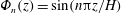
In (2.11),
 $E_{n}$
is the vertically averaged horizontal energy flux in the
$E_{n}$
is the vertically averaged horizontal energy flux in the
 $n\text{th}$
mode. The energy flux
$n\text{th}$
mode. The energy flux
 $E_{n}$
is assumed to be independent of time, thus implying that we are constructing a steady-state weakly nonlinear solution. Corresponding solutions to the equations in (2.9) and (2.10) are
$E_{n}$
is assumed to be independent of time, thus implying that we are constructing a steady-state weakly nonlinear solution. Corresponding solutions to the equations in (2.9) and (2.10) are
 $$\begin{eqnarray}\displaystyle & \displaystyle \unicode[STIX]{x1D70C}_{1}={\displaystyle \frac{1}{\unicode[STIX]{x1D714}}}{\displaystyle \frac{\text{d}\unicode[STIX]{x1D70C}_{0}}{\text{d}z}}\mathop{\sum }_{n=1}^{\infty }\sqrt{{\displaystyle \frac{2\unicode[STIX]{x1D714}k_{n}E_{n}}{\displaystyle \unicode[STIX]{x1D70C}^{\ast }(\unicode[STIX]{x1D714}^{2}-f^{2})\displaystyle \int _{0}^{H}\left({\displaystyle \frac{\text{d}\unicode[STIX]{x1D6F7}_{n}}{\text{d}z}}\right)^{2}\text{d}z}}}\,k_{n}\unicode[STIX]{x1D6F7}_{n}(z)\cos (k_{n}x-\unicode[STIX]{x1D714}t+\unicode[STIX]{x1D6FC}_{n}), & \displaystyle\end{eqnarray}$$
 $$\begin{eqnarray}\displaystyle & \displaystyle v_{1}={\displaystyle \frac{-f}{\unicode[STIX]{x1D714}}}\mathop{\sum }_{n=1}^{\infty }\sqrt{{\displaystyle \frac{2\unicode[STIX]{x1D714}k_{n}E_{n}}{\displaystyle \unicode[STIX]{x1D70C}^{\ast }(\unicode[STIX]{x1D714}^{2}-f^{2})\displaystyle \int _{0}^{H}\left({\displaystyle \frac{\text{d}\unicode[STIX]{x1D6F7}_{n}}{\text{d}z}}\right)^{2}\text{d}z}}}\,{\displaystyle \frac{\text{d}\unicode[STIX]{x1D6F7}_{n}}{\text{d}z}}\sin (k_{n}x-\unicode[STIX]{x1D714}t+\unicode[STIX]{x1D6FC}_{n}). & \displaystyle\end{eqnarray}$$
Substituting
 $(\unicode[STIX]{x1D713}_{0},\unicode[STIX]{x1D70C}_{0},v_{0})$
into (2.5), the
$(\unicode[STIX]{x1D713}_{0},\unicode[STIX]{x1D70C}_{0},v_{0})$
into (2.5), the
 $\mathit{O}(\unicode[STIX]{x1D716}^{2})$
terms generate the governing equation for
$\mathit{O}(\unicode[STIX]{x1D716}^{2})$
terms generate the governing equation for
 $\unicode[STIX]{x1D713}_{2}$
as
$\unicode[STIX]{x1D713}_{2}$
as
 $$\begin{eqnarray}{\displaystyle \frac{\unicode[STIX]{x2202}^{2}}{\unicode[STIX]{x2202}t^{2}}}(\unicode[STIX]{x1D6FB}^{2}\unicode[STIX]{x1D713}_{2})+f^{2}{\displaystyle \frac{\unicode[STIX]{x2202}^{2}\unicode[STIX]{x1D713}_{2}}{\unicode[STIX]{x2202}z^{2}}}+N^{2}{\displaystyle \frac{\unicode[STIX]{x2202}^{2}\unicode[STIX]{x1D713}_{2}}{\unicode[STIX]{x2202}x^{2}}}={\displaystyle \frac{g}{\unicode[STIX]{x1D70C}^{\ast }}}{\displaystyle \frac{\unicode[STIX]{x2202}}{\unicode[STIX]{x2202}x}}[J(\unicode[STIX]{x1D713}_{1},\unicode[STIX]{x1D70C}_{1})]-{\displaystyle \frac{\unicode[STIX]{x2202}}{\unicode[STIX]{x2202}t}}[J(\unicode[STIX]{x1D713}_{1},\unicode[STIX]{x1D6FB}^{2}\unicode[STIX]{x1D713}_{1})]+f{\displaystyle \frac{\unicode[STIX]{x2202}}{\unicode[STIX]{x2202}z}}[J(\unicode[STIX]{x1D713}_{1},v_{1})].\end{eqnarray}$$
The right-hand side of (2.15), which we denote by
 $R$
, is evaluated by substituting the solutions for
$R$
, is evaluated by substituting the solutions for
 $(\unicode[STIX]{x1D713}_{1},\unicode[STIX]{x1D70C}_{1},v_{1})$
from expressions (2.11), (2.13) and (2.14) to give
$(\unicode[STIX]{x1D713}_{1},\unicode[STIX]{x1D70C}_{1},v_{1})$
from expressions (2.11), (2.13) and (2.14) to give
 $$\begin{eqnarray}\left.\begin{array}{@{}rcl@{}}R\, & =\, & \displaystyle \mathop{\sum }_{m=1}^{\infty }\mathop{\sum }_{n=1}^{\infty }[\!A_{mn}\cos ((k_{m}+k_{n})x-2\unicode[STIX]{x1D714}t+\unicode[STIX]{x1D6FC}_{m}+\unicode[STIX]{x1D6FC}_{n})\\ \, & \, & +\,B_{mn}\cos ((k_{m}-k_{n})x+\unicode[STIX]{x1D6FC}_{m}-\unicode[STIX]{x1D6FC}_{n})\!],\\ A_{mn}(z)\, & =\, & \displaystyle {\displaystyle \frac{2\unicode[STIX]{x1D714}}{\unicode[STIX]{x1D70C}^{\ast }(\unicode[STIX]{x1D714}^{2}-f^{2})}}\sqrt{{\displaystyle \frac{k_{m}k_{n}E_{m}E_{n}}{\displaystyle \int _{0}^{H}\left({\displaystyle \frac{\text{d}\unicode[STIX]{x1D6F7}_{m}}{\text{d}z}}\right)^{2}\text{d}z\displaystyle \int _{0}^{H}\left({\displaystyle \frac{\text{d}\unicode[STIX]{x1D6F7}_{n}}{\text{d}z}}\right)^{2}\text{d}z}}}\\ \, & \, & \times \,\left({\displaystyle \frac{\unicode[STIX]{x1D6F7}_{m}k_{m}k_{n}}{2\unicode[STIX]{x1D714}}}\left[N^{2}{\displaystyle \frac{\text{d}\unicode[STIX]{x1D6F7}_{n}}{\text{d}z}}+{\displaystyle \frac{\text{d}(N^{2})}{\text{d}z}}\unicode[STIX]{x1D6F7}_{n}\right](k_{m}+k_{n})-{\displaystyle \frac{\unicode[STIX]{x1D6F7}_{n}k_{n}^{2}}{2\unicode[STIX]{x1D714}}}{\displaystyle \frac{\text{d}\unicode[STIX]{x1D6F7}_{m}}{\text{d}z}}N^{2}(k_{m}+k_{n})\right.\\ \, & \, & -\,\unicode[STIX]{x1D714}\left[\unicode[STIX]{x1D6F7}_{m}k_{m}\left(\displaystyle {\displaystyle \frac{\text{d}^{3}\unicode[STIX]{x1D6F7}_{n}}{\text{d}z^{3}}}-k_{n}^{2}{\displaystyle \frac{\text{d}\unicode[STIX]{x1D6F7}_{n}}{\text{d}z}}\right)-{\displaystyle \frac{\text{d}\unicode[STIX]{x1D6F7}_{m}}{\text{d}z}}k_{n}\left({\displaystyle \frac{\text{d}^{2}\unicode[STIX]{x1D6F7}_{n}}{\text{d}z^{2}}}-k_{n}^{2}\unicode[STIX]{x1D6F7}_{n}\right)\right]\\ \, & \, & -\displaystyle \left.{\displaystyle \frac{f^{2}}{2\unicode[STIX]{x1D714}}}\left[k_{m}{\displaystyle \frac{\text{d}\unicode[STIX]{x1D6F7}_{m}}{\text{d}z}}{\displaystyle \frac{\text{d}^{2}\unicode[STIX]{x1D6F7}_{n}}{\text{d}z^{2}}}+k_{m}\unicode[STIX]{x1D6F7}_{m}{\displaystyle \frac{\text{d}^{3}\unicode[STIX]{x1D6F7}_{n}}{\text{d}z^{3}}}-k_{n}{\displaystyle \frac{\text{d}^{2}\unicode[STIX]{x1D6F7}_{m}}{\text{d}z^{2}}}{\displaystyle \frac{\text{d}\unicode[STIX]{x1D6F7}_{n}}{\text{d}z}}-k_{n}{\displaystyle \frac{\text{d}^{2}\unicode[STIX]{x1D6F7}_{n}}{\text{d}z^{2}}}{\displaystyle \frac{\text{d}\unicode[STIX]{x1D6F7}_{m}}{\text{d}z}}\right]\right),\\ B_{mn}(z)\, & =\, & \displaystyle {\displaystyle \frac{2\unicode[STIX]{x1D714}}{\unicode[STIX]{x1D70C}^{\ast }(\unicode[STIX]{x1D714}^{2}-f^{2})}}\sqrt{{\displaystyle \frac{k_{m}k_{n}E_{m}E_{n}}{\displaystyle \int _{0}^{H}\left({\displaystyle \frac{\text{d}\unicode[STIX]{x1D6F7}_{m}}{\text{d}z}}\right)^{2}\text{d}z\displaystyle \int _{0}^{H}\left({\displaystyle \frac{\text{d}\unicode[STIX]{x1D6F7}_{n}}{\text{d}z}}\right)^{2}\text{d}z}}}\\ \, & \, & \times \,\left({\displaystyle \frac{\unicode[STIX]{x1D6F7}_{m}k_{m}k_{n}}{2\unicode[STIX]{x1D714}}}\left[N^{2}{\displaystyle \frac{\text{d}\unicode[STIX]{x1D6F7}_{n}}{\text{d}z}}+{\displaystyle \frac{\text{d}(N^{2})}{\text{d}z}}\unicode[STIX]{x1D6F7}_{n}\right](k_{m}-k_{n})+{\displaystyle \frac{\unicode[STIX]{x1D6F7}_{n}k_{n}^{2}}{2\unicode[STIX]{x1D714}}}{\displaystyle \frac{\text{d}\unicode[STIX]{x1D6F7}_{m}}{\text{d}z}}N^{2}(k_{m}-k_{n})\right.\\ \, & \, & +\,\left.{\displaystyle \frac{f^{2}}{2\unicode[STIX]{x1D714}}}\left[k_{m}{\displaystyle \frac{\text{d}\unicode[STIX]{x1D6F7}_{m}}{\text{d}z}}{\displaystyle \frac{\text{d}^{2}\unicode[STIX]{x1D6F7}_{n}}{\text{d}z^{2}}}+k_{m}\unicode[STIX]{x1D6F7}_{m}{\displaystyle \frac{\text{d}^{3}\unicode[STIX]{x1D6F7}_{n}}{\text{d}z^{3}}}+k_{n}{\displaystyle \frac{\text{d}^{2}\unicode[STIX]{x1D6F7}_{m}}{\text{d}z^{2}}}{\displaystyle \frac{\text{d}\unicode[STIX]{x1D6F7}_{n}}{\text{d}z}}+k_{n}{\displaystyle \frac{\text{d}^{2}\unicode[STIX]{x1D6F7}_{n}}{\text{d}z^{2}}}{\displaystyle \frac{\text{d}\unicode[STIX]{x1D6F7}_{m}}{\text{d}z}}\right]\right).\end{array}\right\}\end{eqnarray}$$
The forcing function
 $R$
results from an interaction between various modes present at leading order, i.e. in the solutions for
$R$
results from an interaction between various modes present at leading order, i.e. in the solutions for
 $\unicode[STIX]{x1D713}_{1},\unicode[STIX]{x1D70C}_{1}$
and
$\unicode[STIX]{x1D713}_{1},\unicode[STIX]{x1D70C}_{1}$
and
 $v_{1}$
. The solution
$v_{1}$
. The solution
 $\unicode[STIX]{x1D713}_{2}$
of the linear equation (2.15) is written in the same form as the two terms in the forcing function
$\unicode[STIX]{x1D713}_{2}$
of the linear equation (2.15) is written in the same form as the two terms in the forcing function
 $R$
:
$R$
:
 $$\begin{eqnarray}\displaystyle \unicode[STIX]{x1D713}_{2} & = & \displaystyle \mathop{\sum }_{m=-\infty }^{\infty }\mathop{\sum }_{n=-\infty }^{\infty }[\!h_{mn}(z)\cos \left((k_{m}+k_{n})x-2\unicode[STIX]{x1D714}t\right.\nonumber\\ \displaystyle & & \displaystyle \left.+\,\unicode[STIX]{x1D6FC}_{m}+\unicode[STIX]{x1D6FC}_{n}\right)+g_{mn}(z)\cos ((k_{m}-k_{n})x+\unicode[STIX]{x1D6FC}_{m}-\unicode[STIX]{x1D6FC}_{n})\!],\end{eqnarray}$$
thus comprising superharmonic waves of frequency
 $2\unicode[STIX]{x1D714}$
(and horizontal wavenumber
$2\unicode[STIX]{x1D714}$
(and horizontal wavenumber
 $k_{m}+k_{n}$
) and time-independent standing waves (and hence a non-zero mean flow) of horizontal wavenumber
$k_{m}+k_{n}$
) and time-independent standing waves (and hence a non-zero mean flow) of horizontal wavenumber
 $k_{m}-k_{n}$
. Substituting the solution form (2.17) into (2.15) generates the governing equation for
$k_{m}-k_{n}$
. Substituting the solution form (2.17) into (2.15) generates the governing equation for
 $h_{mn}(z)$
and
$h_{mn}(z)$
and
 $g_{mn}(z)$
. For a given modal pair
$g_{mn}(z)$
. For a given modal pair
 $(m,\,n)$
, we define
$(m,\,n)$
, we define
 $\bar{h}_{mn}(z)=h_{mn}(z)+h_{nm}(z)$
and
$\bar{h}_{mn}(z)=h_{mn}(z)+h_{nm}(z)$
and
 $\bar{g}_{mn}(z)=g_{mn}(z)+g_{nm}(z)$
, which describe the vertical structure of the resulting superharmonic and time-independent terms, respectively, in
$\bar{g}_{mn}(z)=g_{mn}(z)+g_{nm}(z)$
, which describe the vertical structure of the resulting superharmonic and time-independent terms, respectively, in
 $\unicode[STIX]{x1D713}_{2}$
. The governing equations for
$\unicode[STIX]{x1D713}_{2}$
. The governing equations for
 $\bar{h}_{mn}(z)$
and
$\bar{h}_{mn}(z)$
and
 $\bar{g}_{mn}(z)$
are
$\bar{g}_{mn}(z)$
are
 $$\begin{eqnarray}\displaystyle & \displaystyle {\displaystyle \frac{\text{d}^{2}\bar{h}_{mn}}{\text{d}z^{2}}}+(k_{m}+k_{n})^{2}{\displaystyle \frac{N^{2}-4\unicode[STIX]{x1D714}^{2}}{4\unicode[STIX]{x1D714}^{2}-f^{2}}}\bar{h}_{mn}=\bar{C}_{mn}, & \displaystyle\end{eqnarray}$$
 $$\begin{eqnarray}\displaystyle & \displaystyle {\displaystyle \frac{\text{d}^{2}\bar{g}_{mn}}{\text{d}z^{2}}}-(k_{m}-k_{n})^{2}{\displaystyle \frac{N^{2}}{f^{2}}}\bar{g}_{mn}=\bar{F}_{mn}, & \displaystyle\end{eqnarray}$$
with the forcing functions being given by
 $\bar{C}_{mn}=-(A_{mn}+A_{nm})/(4\unicode[STIX]{x1D714}^{2}-f^{2})$
and
$\bar{C}_{mn}=-(A_{mn}+A_{nm})/(4\unicode[STIX]{x1D714}^{2}-f^{2})$
and
 $\bar{F}_{mn}=(B_{mn}+B_{nm})/f^{2}$
;
$\bar{F}_{mn}=(B_{mn}+B_{nm})/f^{2}$
;
 $\bar{h}_{mn}(z)$
and
$\bar{h}_{mn}(z)$
and
 $\bar{g}_{mn}(z)$
satisfy the boundary conditions
$\bar{g}_{mn}(z)$
satisfy the boundary conditions
 $\bar{h}_{mn}(z=0)=\bar{h}_{mn}(z=H)=\bar{g}_{mn}(z=0)=\bar{g}_{mn}(z=H)=0$
. A brief discussion on the mean flow vertical structure
$\bar{h}_{mn}(z=0)=\bar{h}_{mn}(z=H)=\bar{g}_{mn}(z=0)=\bar{g}_{mn}(z=H)=0$
. A brief discussion on the mean flow vertical structure
 $\bar{g}_{mn}(z)$
is given in appendix A. In this paper, we focus our attention on
$\bar{g}_{mn}(z)$
is given in appendix A. In this paper, we focus our attention on
 $\bar{h}_{mn}(z)$
, the vertical structure of the superharmonic nonlinear term.
$\bar{h}_{mn}(z)$
, the vertical structure of the superharmonic nonlinear term.
For a given non-uniform stratification
 $N(z)$
,
$N(z)$
,
 $\bar{h}_{mn}(z)$
is calculated numerically by solving equation (2.18) along with the boundary conditions as a boundary value problem using the in-built Matlab function bvp4c. For a fixed stratification profile and
$\bar{h}_{mn}(z)$
is calculated numerically by solving equation (2.18) along with the boundary conditions as a boundary value problem using the in-built Matlab function bvp4c. For a fixed stratification profile and
 $(m,\,n)$
, we compute
$(m,\,n)$
, we compute
 $\bar{h}_{mn}^{max}=\max (|\bar{h}_{mn}(z)|)$
on a grid of
$\bar{h}_{mn}^{max}=\max (|\bar{h}_{mn}(z)|)$
on a grid of
 $400\times 200$
uniformly spaced points on the plane of
$400\times 200$
uniformly spaced points on the plane of
 $(\unicode[STIX]{x1D714}/N_{0},f/\unicode[STIX]{x1D714})\in [0.01,0.99]\times [0.01,0.99]$
. For a given modal pair
$(\unicode[STIX]{x1D714}/N_{0},f/\unicode[STIX]{x1D714})\in [0.01,0.99]\times [0.01,0.99]$
. For a given modal pair
 $(m,\,n)$
, we identify all the curves (referred to as the maxima curves) on the
$(m,\,n)$
, we identify all the curves (referred to as the maxima curves) on the
 $(\unicode[STIX]{x1D714}/N_{0},f/\unicode[STIX]{x1D714})$
plane along which
$(\unicode[STIX]{x1D714}/N_{0},f/\unicode[STIX]{x1D714})$
plane along which
 $\bar{h}_{mn}^{max}$
is a local maximum in a direction that is locally orthogonal to the curve. As discussed in § 3.2, we further verify that
$\bar{h}_{mn}^{max}$
is a local maximum in a direction that is locally orthogonal to the curve. As discussed in § 3.2, we further verify that
 $\bar{h}_{mn}^{max}$
diverges in a very small neighbourhood around the maxima curves, which are henceforth termed divergence curves in the rest of this paper. Along every divergence curve we identify, the mode number
$\bar{h}_{mn}^{max}$
diverges in a very small neighbourhood around the maxima curves, which are henceforth termed divergence curves in the rest of this paper. Along every divergence curve we identify, the mode number
 $s$
associated with the corresponding higher harmonic wave is calculated as
$s$
associated with the corresponding higher harmonic wave is calculated as
 $s=n_{z}+1$
, where
$s=n_{z}+1$
, where
 $n_{z}$
is the number of zeros for
$n_{z}$
is the number of zeros for
 $\bar{h}_{mn}(z)$
in
$\bar{h}_{mn}(z)$
in
 $z\in (0,H)$
.
$z\in (0,H)$
.
3 Results
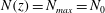
We present results for an ocean-like non-uniform stratification profile
 $N(z)$
(figure 1
a):
$N(z)$
(figure 1
a):
 $$\begin{eqnarray}N(z)=N_{0}+(N_{max}-N_{0})\exp \left(-{\displaystyle \frac{(z-z_{c})^{2}}{\unicode[STIX]{x1D70E}^{2}}}\right),\quad 0\leqslant z\leqslant H,\end{eqnarray}$$
where
 $N_{0}$
is the deep ocean uniform stratification and
$N_{0}$
is the deep ocean uniform stratification and
 $z_{c}$
is the centre of the pycnocline whose characteristic width and maximum stratification are
$z_{c}$
is the centre of the pycnocline whose characteristic width and maximum stratification are
 $\unicode[STIX]{x1D70E}$
and
$\unicode[STIX]{x1D70E}$
and
 $N_{max}$
, respectively;
$N_{max}$
, respectively;
 $z_{c}=3400~\text{m}$
and
$z_{c}=3400~\text{m}$
and
 $\unicode[STIX]{x1D70E}=250~\text{m}$
are fixed throughout this paper, whereas
$\unicode[STIX]{x1D70E}=250~\text{m}$
are fixed throughout this paper, whereas
 $N_{max}$
is varied to study the effects of pycnocline strength in § 3.2. For the specific case of
$N_{max}$
is varied to study the effects of pycnocline strength in § 3.2. For the specific case of
 $N_{0}=6\times 10^{-4}~\text{rad}~\text{s}^{-1}$
,
$N_{0}=6\times 10^{-4}~\text{rad}~\text{s}^{-1}$
,
 $N_{max}=10N_{0}$
,
$N_{max}=10N_{0}$
,
 $\unicode[STIX]{x1D714}=1.4053\times 10^{-4}~\text{rad}~\text{s}^{-1}$
and
$\unicode[STIX]{x1D714}=1.4053\times 10^{-4}~\text{rad}~\text{s}^{-1}$
and
 $f=0$
, the vertical mode shapes
$f=0$
, the vertical mode shapes
 $\unicode[STIX]{x1D6F7}_{n}(z)$
(calculated by solving (2.12) numerically) for
$\unicode[STIX]{x1D6F7}_{n}(z)$
(calculated by solving (2.12) numerically) for
 $n=1,2,3$
are shown in figure 1(b);
$n=1,2,3$
are shown in figure 1(b);
 $\unicode[STIX]{x1D6F7}_{7}$
is plotted in figure 1(c). All the modes assume a sinusoidal form in the uniformly stratified deep ocean, and contain smaller vertical length scales in the pycnocline region.
$\unicode[STIX]{x1D6F7}_{7}$
is plotted in figure 1(c). All the modes assume a sinusoidal form in the uniformly stratified deep ocean, and contain smaller vertical length scales in the pycnocline region.

Figure 1. (a) The ocean-like stratification profile we consider in § 3. For the specific case of
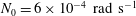 $N_{0}=6\times 10^{-4}~\text{rad}~\text{s}^{-1}$
,
$N_{0}=6\times 10^{-4}~\text{rad}~\text{s}^{-1}$
,
 $N_{max}=10N_{0}$
,
$N_{max}=10N_{0}$
,
 $\unicode[STIX]{x1D714}=1.4053\times 10^{-4}~\text{rad}~\text{s}^{-1}$
and
$\unicode[STIX]{x1D714}=1.4053\times 10^{-4}~\text{rad}~\text{s}^{-1}$
and
 $f=0$
, the vertical mode shapes
$f=0$
, the vertical mode shapes
 $\unicode[STIX]{x1D6F7}_{n}(z)$
for (b)
$\unicode[STIX]{x1D6F7}_{n}(z)$
for (b)
 $n=1,2,3$
and (c)
$n=1,2,3$
and (c)
 $n=7$
are shown. All the modes in (b) and (c) correspond to
$n=7$
are shown. All the modes in (b) and (c) correspond to
 $E_{n}=1~\text{W}~\text{m}^{-1}$
.
$E_{n}=1~\text{W}~\text{m}^{-1}$
.
3.1 Uniform stratification (
 $m\neq n$
)
$m\neq n$
)

For a uniform stratification, i.e.
 $N(z)=N_{max}=N_{0}$
where
$N(z)=N_{max}=N_{0}$
where
 $N_{0}$
is constant, equation (2.12) is solved analytically with the boundary conditions
$N_{0}$
is constant, equation (2.12) is solved analytically with the boundary conditions
 $\unicode[STIX]{x1D6F7}_{n}(z=0)=\unicode[STIX]{x1D6F7}_{n}(z=H)=0$
to obtain
$\unicode[STIX]{x1D6F7}_{n}(z=0)=\unicode[STIX]{x1D6F7}_{n}(z=H)=0$
to obtain
 $\unicode[STIX]{x1D6F7}_{n}(z)=\sin (n\unicode[STIX]{x03C0}z/H)$
and
$\unicode[STIX]{x1D6F7}_{n}(z)=\sin (n\unicode[STIX]{x03C0}z/H)$
and
 $k_{n}=n\unicode[STIX]{x03C0}/(H\cot \unicode[STIX]{x1D703})$
, where
$k_{n}=n\unicode[STIX]{x03C0}/(H\cot \unicode[STIX]{x1D703})$
, where
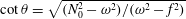 $\cot \unicode[STIX]{x1D703}=\sqrt{(N_{0}^{2}-\unicode[STIX]{x1D714}^{2})/(\unicode[STIX]{x1D714}^{2}-f^{2})}$
. Substituting for
$\cot \unicode[STIX]{x1D703}=\sqrt{(N_{0}^{2}-\unicode[STIX]{x1D714}^{2})/(\unicode[STIX]{x1D714}^{2}-f^{2})}$
. Substituting for
 $\unicode[STIX]{x1D6F7}_{n}(z)$
and
$\unicode[STIX]{x1D6F7}_{n}(z)$
and
 $k_{n}$
, the particular solutions of (2.18) and (2.19) are
$k_{n}$
, the particular solutions of (2.18) and (2.19) are
 $$\begin{eqnarray}\bar{h}_{mn}=\bar{I}_{mn}\sin \left({\displaystyle \frac{(m-n)\unicode[STIX]{x03C0}z}{H}}\right),\quad \bar{g}_{mn}=\bar{J}_{mn}\sin \left({\displaystyle \frac{(m+n)\unicode[STIX]{x03C0}z}{H}}\right),\end{eqnarray}$$
where
 $$\begin{eqnarray}\bar{I}_{mn}={\displaystyle \frac{4\unicode[STIX]{x03C0}\unicode[STIX]{x1D714}\sqrt{mnE_{m}E_{n}}}{\unicode[STIX]{x1D70C}^{\ast }H^{2}(\unicode[STIX]{x1D714}^{2}-f^{2})}}\left({\displaystyle \frac{(m^{2}-n^{2})\left({\displaystyle \frac{N_{0}^{2}}{2\unicode[STIX]{x1D714}\cot ^{2}\unicode[STIX]{x1D703}}}+{\displaystyle \frac{\unicode[STIX]{x1D714}(N_{0}^{2}-f^{2})}{(\unicode[STIX]{x1D714}^{2}-f^{2})\cot ^{2}\unicode[STIX]{x1D703}}}+{\displaystyle \frac{f^{2}}{2\unicode[STIX]{x1D714}}}\right)}{(m+n)^{2}(N_{0}^{2}-4\unicode[STIX]{x1D714}^{2}){-}(m-n)^{2}(4\unicode[STIX]{x1D714}^{2}-f^{2})\cot ^{2}\unicode[STIX]{x1D703}}}\right),\end{eqnarray}$$
 $$\begin{eqnarray}\bar{J}_{mn}={\displaystyle \frac{2\unicode[STIX]{x03C0}\sqrt{mnE_{m}E_{n}}}{\unicode[STIX]{x1D70C}^{\ast }H^{2}(\unicode[STIX]{x1D714}^{2}-f^{2})\cot ^{2}\unicode[STIX]{x1D703}}}.\end{eqnarray}$$
For a given
 $(m,\,n)$
, the coefficient
$(m,\,n)$
, the coefficient
 $\bar{I}_{mn}$
in (3.2), and hence the superharmonic part of the weakly nonlinear solution, diverges if the condition
$\bar{I}_{mn}$
in (3.2), and hence the superharmonic part of the weakly nonlinear solution, diverges if the condition
 $(m+n)^{2}(N_{0}^{2}-4\unicode[STIX]{x1D714}^{2}){-}(m-n)^{2}(4\unicode[STIX]{x1D714}^{2}-f^{2})\cot ^{2}\unicode[STIX]{x1D703}=0$
is satisfied. Therefore, for fixed values of
$(m+n)^{2}(N_{0}^{2}-4\unicode[STIX]{x1D714}^{2}){-}(m-n)^{2}(4\unicode[STIX]{x1D714}^{2}-f^{2})\cot ^{2}\unicode[STIX]{x1D703}=0$
is satisfied. Therefore, for fixed values of
 $m$
,
$m$
,
 $n$
and
$n$
and
 $f/\unicode[STIX]{x1D714}$
, the weakly nonlinear steady-state solution diverges for values of
$f/\unicode[STIX]{x1D714}$
, the weakly nonlinear steady-state solution diverges for values of
 $\unicode[STIX]{x1D714}/N_{0}$
given by
$\unicode[STIX]{x1D714}/N_{0}$
given by
 $$\begin{eqnarray}{\displaystyle \frac{\unicode[STIX]{x1D714}^{2}}{N_{0}^{2}}}={\displaystyle \frac{(m+n)^{2}-(m-n)^{2}(4-f^{2}/\unicode[STIX]{x1D714}^{2})/(1-f^{2}/\unicode[STIX]{x1D714}^{2})}{4(m+n)^{2}-(m-n)^{2}(4-f^{2}/\unicode[STIX]{x1D714}^{2})/(1-f^{2}/\unicode[STIX]{x1D714}^{2})}},\end{eqnarray}$$
implying that no small-amplitude internal waves with non-zero strength in modes
 $m$
and
$m$
and
 $n$
at the frequency given by (3.5) can persist in their linear form. In the limit of
$n$
at the frequency given by (3.5) can persist in their linear form. In the limit of
 $f=0$
, expression (3.5) is the same as what has been derived by Thorpe (Reference Thorpe1966). The expression in (3.5) can be equivalently derived by requiring the vertical mode number
$f=0$
, expression (3.5) is the same as what has been derived by Thorpe (Reference Thorpe1966). The expression in (3.5) can be equivalently derived by requiring the vertical mode number
 $|m-n|$
at frequency
$|m-n|$
at frequency
 $2\unicode[STIX]{x1D714}$
to correspond to a horizontal wavenumber of
$2\unicode[STIX]{x1D714}$
to correspond to a horizontal wavenumber of
 $k_{m}+k_{n}$
, i.e. the two primary modes and the superharmonic wave form an internal wave resonant triad. It is noteworthy that there exists no such closed-form expressions or any other criterion for verification of resonance in non-uniform stratifications.
$k_{m}+k_{n}$
, i.e. the two primary modes and the superharmonic wave form an internal wave resonant triad. It is noteworthy that there exists no such closed-form expressions or any other criterion for verification of resonance in non-uniform stratifications.
For at least one value of
 $f/\unicode[STIX]{x1D714}$
to exist in the range
$f/\unicode[STIX]{x1D714}$
to exist in the range
 $0\leqslant f/\unicode[STIX]{x1D714}<1$
such that the corresponding
$0\leqslant f/\unicode[STIX]{x1D714}<1$
such that the corresponding
 $\unicode[STIX]{x1D714}/N_{0}$
given by the expression in (3.5) satisfies
$\unicode[STIX]{x1D714}/N_{0}$
given by the expression in (3.5) satisfies
 $0<\unicode[STIX]{x1D714}/N_{0}<1$
, one requires the condition
$0<\unicode[STIX]{x1D714}/N_{0}<1$
, one requires the condition
 $(m+n)^{2}>4(m-n)^{2}$
to be satisfied. In other words, assuming a fixed frequency
$(m+n)^{2}>4(m-n)^{2}$
to be satisfied. In other words, assuming a fixed frequency
 $\unicode[STIX]{x1D714}$
in the leading-order internal wave solution, divergence of the weakly nonlinear steady-state solution occurs for some
$\unicode[STIX]{x1D714}$
in the leading-order internal wave solution, divergence of the weakly nonlinear steady-state solution occurs for some
 $(\unicode[STIX]{x1D714}/N_{0},f/\unicode[STIX]{x1D714})$
(in the wave propagation regime) based on the interaction between modes
$(\unicode[STIX]{x1D714}/N_{0},f/\unicode[STIX]{x1D714})$
(in the wave propagation regime) based on the interaction between modes
 $m$
and
$m$
and
 $n$
that satisfy
$n$
that satisfy
 $$\begin{eqnarray}(m/3)<n<3m,\quad m\neq n.\end{eqnarray}$$

Figure 2.
 $\text{log}_{10}[\bar{h}_{mn}^{max}]$
plotted as a function of
$\text{log}_{10}[\bar{h}_{mn}^{max}]$
plotted as a function of
 $\unicode[STIX]{x1D714}/N_{0}$
and
$\unicode[STIX]{x1D714}/N_{0}$
and
 $f/\unicode[STIX]{x1D714}$
for
$f/\unicode[STIX]{x1D714}$
for
 $(m,\,n)=(1,2)$
(column 1),
$(m,\,n)=(1,2)$
(column 1),
 $(2,3)$
(column 2) and
$(2,3)$
(column 2) and
 $(2,\,5)$
(column 3). The first, second, third and fourth rows correspond to
$(2,\,5)$
(column 3). The first, second, third and fourth rows correspond to
 $N_{max}=N_{0}$
(uniform stratification),
$N_{max}=N_{0}$
(uniform stratification),
 $1.5N_{0},4N_{0}$
and
$1.5N_{0},4N_{0}$
and
 $10N_{0}$
, respectively, in the stratification profile given by (3.1). The energy fluxes for each plot are fixed at
$10N_{0}$
, respectively, in the stratification profile given by (3.1). The energy fluxes for each plot are fixed at
 $(E_{m},E_{n})=(0.9,0.1)~\text{W}~\text{m}^{-1}$
. The mode numbers associated with the higher harmonic wave along the divergence curves are indicated by the encircled numbers. Note that the common colour bar (shown next to (a)) is saturated at a value of 1, hence making some of the divergence curves appear white.
$(E_{m},E_{n})=(0.9,0.1)~\text{W}~\text{m}^{-1}$
. The mode numbers associated with the higher harmonic wave along the divergence curves are indicated by the encircled numbers. Note that the common colour bar (shown next to (a)) is saturated at a value of 1, hence making some of the divergence curves appear white.
In figure 2, we plot the variation of
 $\log _{10}[\bar{h}_{mn}^{max}]$
as a function of
$\log _{10}[\bar{h}_{mn}^{max}]$
as a function of
 $\unicode[STIX]{x1D714}/N_{0}$
and
$\unicode[STIX]{x1D714}/N_{0}$
and
 $f/\unicode[STIX]{x1D714}$
for fixed values of
$f/\unicode[STIX]{x1D714}$
for fixed values of
 $(E_{m},E_{n})=(0.9,0.1)~\text{W}~\text{m}^{-1}$
, where
$(E_{m},E_{n})=(0.9,0.1)~\text{W}~\text{m}^{-1}$
, where
 $\bar{h}_{mn}^{max}=\max (|\bar{h}_{mn}(z)|)$
. Figure 2(a–c) correspond to
$\bar{h}_{mn}^{max}=\max (|\bar{h}_{mn}(z)|)$
. Figure 2(a–c) correspond to
 $(m,\,n)=(1,2),(2,3)$
and
$(m,\,n)=(1,2),(2,3)$
and
 $(2,\,5)$
, respectively, for the uniform stratification (
$(2,\,5)$
, respectively, for the uniform stratification (
 $N_{max}=N_{0}$
). As shown in figure 2(a), there is a difference of a few orders of magnitude between regions close to and far from the divergence curve, which is described by (3.5). The divergence occurs at
$N_{max}=N_{0}$
). As shown in figure 2(a), there is a difference of a few orders of magnitude between regions close to and far from the divergence curve, which is described by (3.5). The divergence occurs at
 $\unicode[STIX]{x1D714}/N_{0}=0.395$
for
$\unicode[STIX]{x1D714}/N_{0}=0.395$
for
 $f/\unicode[STIX]{x1D714}=0$
and then moves towards smaller values of
$f/\unicode[STIX]{x1D714}=0$
and then moves towards smaller values of
 $\unicode[STIX]{x1D714}/N_{0}$
as
$\unicode[STIX]{x1D714}/N_{0}$
as
 $f/\unicode[STIX]{x1D714}$
is increased from zero. At approximately
$f/\unicode[STIX]{x1D714}$
is increased from zero. At approximately
 $f/\unicode[STIX]{x1D714}\approx 0.79$
, the curve is almost horizontal, implying that strong nonlinear effects would occur over a wide range of
$f/\unicode[STIX]{x1D714}\approx 0.79$
, the curve is almost horizontal, implying that strong nonlinear effects would occur over a wide range of
 $\unicode[STIX]{x1D714}/N_{0}$
if modes 1 and 2 are simultaneously present. The peak occurring at the divergence curve is quite sharp if either
$\unicode[STIX]{x1D714}/N_{0}$
if modes 1 and 2 are simultaneously present. The peak occurring at the divergence curve is quite sharp if either
 $\unicode[STIX]{x1D714}/N_{0}$
or
$\unicode[STIX]{x1D714}/N_{0}$
or
 $f/\unicode[STIX]{x1D714}$
is close to zero. In contrast, noticeably larger regions around the divergence curve correspond to large
$f/\unicode[STIX]{x1D714}$
is close to zero. In contrast, noticeably larger regions around the divergence curve correspond to large
 $\bar{h}_{mn}^{max}$
for values of
$\bar{h}_{mn}^{max}$
for values of
 $\unicode[STIX]{x1D714}/N_{0}$
and
$\unicode[STIX]{x1D714}/N_{0}$
and
 $f/\unicode[STIX]{x1D714}$
away from zero, thus making the occurrence of strong nonlinear effects more likely. As evident in the solution for
$f/\unicode[STIX]{x1D714}$
away from zero, thus making the occurrence of strong nonlinear effects more likely. As evident in the solution for
 $\bar{h}_{mn}(z)$
in (3.2), the mode number of the higher harmonic wave on the divergence curves in a uniform stratification is always
$\bar{h}_{mn}(z)$
in (3.2), the mode number of the higher harmonic wave on the divergence curves in a uniform stratification is always
 $|m-n|$
.
$|m-n|$
.
For
 $(m,\,n)=(2,3)$
, shown in figure 2(b), the divergence curve occurs for larger values of
$(m,\,n)=(2,3)$
, shown in figure 2(b), the divergence curve occurs for larger values of
 $\unicode[STIX]{x1D714}/N_{0}$
and
$\unicode[STIX]{x1D714}/N_{0}$
and
 $f/\unicode[STIX]{x1D714}$
compared to the case of
$f/\unicode[STIX]{x1D714}$
compared to the case of
 $(m,\,n)=(1,2)$
. Interestingly, for
$(m,\,n)=(1,2)$
. Interestingly, for
 $f/\unicode[STIX]{x1D714}\approx 0.935$
, a wide range of values for
$f/\unicode[STIX]{x1D714}\approx 0.935$
, a wide range of values for
 $\unicode[STIX]{x1D714}/N_{0}$
corresponds to infinitely large
$\unicode[STIX]{x1D714}/N_{0}$
corresponds to infinitely large
 $\bar{h}_{23}(z)$
; similarly, for
$\bar{h}_{23}(z)$
; similarly, for
 $\unicode[STIX]{x1D714}/N_{0}\approx 0.468$
, a wide range of
$\unicode[STIX]{x1D714}/N_{0}\approx 0.468$
, a wide range of
 $f/\unicode[STIX]{x1D714}$
corresponds to large magnitudes of
$f/\unicode[STIX]{x1D714}$
corresponds to large magnitudes of
 $\bar{h}_{23}(z)$
. The case of
$\bar{h}_{23}(z)$
. The case of
 $(m,\,n)=(2,5)$
, shown in figure 2(c), is similar to that of
$(m,\,n)=(2,5)$
, shown in figure 2(c), is similar to that of
 $(m,\,n)=(1,2)$
but with the divergence curve occurring at smaller values of
$(m,\,n)=(1,2)$
but with the divergence curve occurring at smaller values of
 $\unicode[STIX]{x1D714}/N_{0}$
and
$\unicode[STIX]{x1D714}/N_{0}$
and
 $f/\unicode[STIX]{x1D714}$
. It is noteworthy that, for the uniform stratification, the divergence curve for
$f/\unicode[STIX]{x1D714}$
. It is noteworthy that, for the uniform stratification, the divergence curve for
 $(m,\,n)=(2,4)$
coincides with that of
$(m,\,n)=(2,4)$
coincides with that of
 $(m,\,n)=(1,2)$
; also, based on condition (3.6), there exist no divergence curves for
$(m,\,n)=(1,2)$
; also, based on condition (3.6), there exist no divergence curves for
 $(1,n\geqslant 3)$
and
$(1,n\geqslant 3)$
and
 $(2,n\geqslant 6)$
. Considering all possible modal interactions, described in detail in appendix C, all the divergence curves together span a significant portion of the plane
$(2,n\geqslant 6)$
. Considering all possible modal interactions, described in detail in appendix C, all the divergence curves together span a significant portion of the plane
 $0<\unicode[STIX]{x1D714}/N_{0}<0.5$
,
$0<\unicode[STIX]{x1D714}/N_{0}<0.5$
,
 $0<f/\unicode[STIX]{x1D714}<1$
. This suggests that modal interactions are highly likely to result in strong nonlinear effects irrespective of the specific values of
$0<f/\unicode[STIX]{x1D714}<1$
. This suggests that modal interactions are highly likely to result in strong nonlinear effects irrespective of the specific values of
 $\unicode[STIX]{x1D714}/N_{0}$
and
$\unicode[STIX]{x1D714}/N_{0}$
and
 $f/\unicode[STIX]{x1D714}$
. For
$f/\unicode[STIX]{x1D714}$
. For
 $\unicode[STIX]{x1D714}/N_{0}>0.5$
in a uniform stratification, the higher harmonic wave at frequency
$\unicode[STIX]{x1D714}/N_{0}>0.5$
in a uniform stratification, the higher harmonic wave at frequency
 $2\unicode[STIX]{x1D714}$
can never represent a propagating internal wave, owing to which no resonant triads (and hence no divergence curves) exist for
$2\unicode[STIX]{x1D714}$
can never represent a propagating internal wave, owing to which no resonant triads (and hence no divergence curves) exist for
 $\unicode[STIX]{x1D714}/N_{0}>0.5$
. In contrast, in a non-uniform stratification with
$\unicode[STIX]{x1D714}/N_{0}>0.5$
. In contrast, in a non-uniform stratification with
 $N_{max}>N_{0}$
, the higher harmonic wave at frequency
$N_{max}>N_{0}$
, the higher harmonic wave at frequency
 $2\unicode[STIX]{x1D714}$
can still represent a propagating internal wave as
$2\unicode[STIX]{x1D714}$
can still represent a propagating internal wave as
 $2\unicode[STIX]{x1D714}/N<1$
somewhere in the pycnocline. Thus, one cannot rule out the possibility of existence of divergence curves for
$2\unicode[STIX]{x1D714}/N<1$
somewhere in the pycnocline. Thus, one cannot rule out the possibility of existence of divergence curves for
 $\unicode[STIX]{x1D714}/N_{0}>0.5$
if
$\unicode[STIX]{x1D714}/N_{0}>0.5$
if
 $N_{max}>N_{0}$
.
$N_{max}>N_{0}$
.
3.2 Non-uniform stratification (
$m\neq n$
)

In figure 2(d–l), we show the variation of
 $\log _{10}[\bar{h}_{mn}^{max}]$
as a function of
$\log _{10}[\bar{h}_{mn}^{max}]$
as a function of
 $\unicode[STIX]{x1D714}/N_{0}$
and
$\unicode[STIX]{x1D714}/N_{0}$
and
 $f/\unicode[STIX]{x1D714}$
for fixed values of
$f/\unicode[STIX]{x1D714}$
for fixed values of
 $(E_{m},E_{n})=(0.9,0.1)~\text{W}~\text{m}^{-1}$
and three different non-uniform stratifications (
$(E_{m},E_{n})=(0.9,0.1)~\text{W}~\text{m}^{-1}$
and three different non-uniform stratifications (
 $N_{max}/N_{0}=1.5,4$
and 10 in the second, third and fourth rows of figure 2, respectively). We consider the same modal pairs as for the uniform stratification plots in figure 2(a–c). For
$N_{max}/N_{0}=1.5,4$
and 10 in the second, third and fourth rows of figure 2, respectively). We consider the same modal pairs as for the uniform stratification plots in figure 2(a–c). For
 $(m,\,n)=(1,2)$
, while the distribution of
$(m,\,n)=(1,2)$
, while the distribution of
 $\log _{10}[\bar{h}_{mn}^{max}]$
for the weak-pycnocline case of
$\log _{10}[\bar{h}_{mn}^{max}]$
for the weak-pycnocline case of
 $N_{max}=1.5N_{0}$
(figure 2
d) is similar to that of
$N_{max}=1.5N_{0}$
(figure 2
d) is similar to that of
 $N_{max}=N_{0}$
, the divergence curve deforms significantly for the intermediate pycnocline strength of
$N_{max}=N_{0}$
, the divergence curve deforms significantly for the intermediate pycnocline strength of
 $N_{max}=4N_{0}$
(figure 2
g) and also extends into the
$N_{max}=4N_{0}$
(figure 2
g) and also extends into the
 $\unicode[STIX]{x1D714}/N_{0}>0.5$
region. The divergence curve then becomes near horizontal for the strong-pycnocline case of
$\unicode[STIX]{x1D714}/N_{0}>0.5$
region. The divergence curve then becomes near horizontal for the strong-pycnocline case of
 $N_{max}=10N_{0}$
(figure 2
j), again spanning the entire range of
$N_{max}=10N_{0}$
(figure 2
j), again spanning the entire range of
 $0<\unicode[STIX]{x1D714}/N_{0}<1$
. For
$0<\unicode[STIX]{x1D714}/N_{0}<1$
. For
 $N_{max}=10N_{0}$
, strong nonlinear effects are therefore expected for all values of
$N_{max}=10N_{0}$
, strong nonlinear effects are therefore expected for all values of
 $\unicode[STIX]{x1D714}/N_{0}$
at
$\unicode[STIX]{x1D714}/N_{0}$
at
 $f/\unicode[STIX]{x1D714}\approx 0.89$
as a result of the low-mode
$f/\unicode[STIX]{x1D714}\approx 0.89$
as a result of the low-mode
 $(1,\,2)$
interaction. As indicated by the encircled numbers on the divergence curves in figure 2(a,d,g,j), we find
$(1,\,2)$
interaction. As indicated by the encircled numbers on the divergence curves in figure 2(a,d,g,j), we find
 $\bar{h}_{mn}(z)$
to correspond to a mode-1 structure (based on the number of zeros in
$\bar{h}_{mn}(z)$
to correspond to a mode-1 structure (based on the number of zeros in
 $z\in (0,H)$
) along these curves for
$z\in (0,H)$
) along these curves for
 $(1,\,2)$
interaction irrespective of
$(1,\,2)$
interaction irrespective of
 $N_{max}$
. Also noteworthy from figure 2(a,d,g,j) is the observation that small
$N_{max}$
. Also noteworthy from figure 2(a,d,g,j) is the observation that small
 $f/\unicode[STIX]{x1D714}$
tends to correspond to no resonant triads for large
$f/\unicode[STIX]{x1D714}$
tends to correspond to no resonant triads for large
 $N_{max}$
.
$N_{max}$
.
For
 $(m,\,n)=(2,3)$
, the number of divergence curves increases to two when
$(m,\,n)=(2,3)$
, the number of divergence curves increases to two when
 $N_{max}$
is increased from
$N_{max}$
is increased from
 $N_{0}$
to
$N_{0}$
to
 $1.5N_{0}$
(figure 2
e). The divergence curve along which
$1.5N_{0}$
(figure 2
e). The divergence curve along which
 $\bar{h}_{mn}(z)$
contains a mode-1 structure becomes near horizontal for
$\bar{h}_{mn}(z)$
contains a mode-1 structure becomes near horizontal for
 $N_{max}=4N_{0}$
(figure 2
h), and is then horizontal and centred around
$N_{max}=4N_{0}$
(figure 2
h), and is then horizontal and centred around
 $f/\unicode[STIX]{x1D714}=0.97$
for
$f/\unicode[STIX]{x1D714}=0.97$
for
 $N_{max}=10N_{0}$
(figure 2
k). The second divergence curve corresponding to a mode-2 structure for the higher harmonic wave tends to become near horizontal at smaller values of
$N_{max}=10N_{0}$
(figure 2
k). The second divergence curve corresponding to a mode-2 structure for the higher harmonic wave tends to become near horizontal at smaller values of
 $f/\unicode[STIX]{x1D714}$
as
$f/\unicode[STIX]{x1D714}$
as
 $N_{max}$
is increased to
$N_{max}$
is increased to
 $10N_{0}$
. In summary, as
$10N_{0}$
. In summary, as
 $N_{max}$
is increased from
$N_{max}$
is increased from
 $1.5N_{0}$
to
$1.5N_{0}$
to
 $10N_{0}$
, both the divergence curves tend to become near horizontal at larger values of
$10N_{0}$
, both the divergence curves tend to become near horizontal at larger values of
 $f/\unicode[STIX]{x1D714}$
, and hence leave the regions of small
$f/\unicode[STIX]{x1D714}$
, and hence leave the regions of small
 $f/\unicode[STIX]{x1D714}$
with no divergence curves. For the higher-modes interaction, i.e.
$f/\unicode[STIX]{x1D714}$
with no divergence curves. For the higher-modes interaction, i.e.
 $(m,\,n)=(2,5)$
shown in figure 2(c,f,i,l), we observe the existence of a larger number of divergence curves. For
$(m,\,n)=(2,5)$
shown in figure 2(c,f,i,l), we observe the existence of a larger number of divergence curves. For
 $N_{max}=1.5N_{0}$
, there are three different divergence curves (with three different modal structures for
$N_{max}=1.5N_{0}$
, there are three different divergence curves (with three different modal structures for
 $\bar{h}_{mn}$
), which is in stark contrast to the existence of only one divergence curve for
$\bar{h}_{mn}$
), which is in stark contrast to the existence of only one divergence curve for
 $N_{max}=N_{0}$
. An additional mode-2 divergence curve emerges in the region of large
$N_{max}=N_{0}$
. An additional mode-2 divergence curve emerges in the region of large
 $\unicode[STIX]{x1D714}/N_{0}$
for
$\unicode[STIX]{x1D714}/N_{0}$
for
 $N_{max}=4N_{0}$
. Similarly, a mode-4 divergence curve occurs at large
$N_{max}=4N_{0}$
. Similarly, a mode-4 divergence curve occurs at large
 $\unicode[STIX]{x1D714}/N_{0}$
for
$\unicode[STIX]{x1D714}/N_{0}$
for
 $N_{max}=10N_{0}$
. It is noteworthy that as
$N_{max}=10N_{0}$
. It is noteworthy that as
 $N_{max}$
increases, the range of
$N_{max}$
increases, the range of
 $\unicode[STIX]{x1D714}/N_{0}$
where the higher harmonic wave at frequency
$\unicode[STIX]{x1D714}/N_{0}$
where the higher harmonic wave at frequency
 $2\unicode[STIX]{x1D714}$
can represent a propagating internal wave increases, thus allowing for additional divergence curves to emerge at large
$2\unicode[STIX]{x1D714}$
can represent a propagating internal wave increases, thus allowing for additional divergence curves to emerge at large
 $\unicode[STIX]{x1D714}/N_{0}$
. An overall summary from figure 2 is that, for a given modal pair
$\unicode[STIX]{x1D714}/N_{0}$
. An overall summary from figure 2 is that, for a given modal pair
 $(m,\,n)$
, regions of small and large
$(m,\,n)$
, regions of small and large
 $f/\unicode[STIX]{x1D714}$
tend to correspond to smaller and larger numbers of resonant triads, respectively.
$f/\unicode[STIX]{x1D714}$
tend to correspond to smaller and larger numbers of resonant triads, respectively.

Figure 3. (a)
 $\text{log}_{10}[\bar{h}_{mn}^{max}]$
plotted as a function of
$\text{log}_{10}[\bar{h}_{mn}^{max}]$
plotted as a function of
 $\unicode[STIX]{x1D714}/N_{0}$
and
$\unicode[STIX]{x1D714}/N_{0}$
and
 $f/\unicode[STIX]{x1D714}$
for
$f/\unicode[STIX]{x1D714}$
for
 $(m,\,n)=(2,5)$
,
$(m,\,n)=(2,5)$
,
 $N_{max}=4N_{0}$
and
$N_{max}=4N_{0}$
and
 $(E_{m},E_{n})=(0.9,0.1)~\text{W}~\text{m}^{-1}$
, the same case as in figure 2(i). Corresponding distributions of (b)
$(E_{m},E_{n})=(0.9,0.1)~\text{W}~\text{m}^{-1}$
, the same case as in figure 2(i). Corresponding distributions of (b)
 $k^{d}=|k_{m}+k_{n}-k_{q}^{2\unicode[STIX]{x1D714}}|/k_{q}^{2\unicode[STIX]{x1D714}}$
and (c)
$k^{d}=|k_{m}+k_{n}-k_{q}^{2\unicode[STIX]{x1D714}}|/k_{q}^{2\unicode[STIX]{x1D714}}$
and (c)
 $\bar{C}_{mn}^{max}/\bar{h}_{mn}^{max}$
are also shown. The various cross-sectional cuts (across the divergence curves) that are considered in the bottom row of panels are shown using black solid lines and indexed from 1 to 12 in (a). (d–f) Detected maximum value of
$\bar{C}_{mn}^{max}/\bar{h}_{mn}^{max}$
are also shown. The various cross-sectional cuts (across the divergence curves) that are considered in the bottom row of panels are shown using black solid lines and indexed from 1 to 12 in (a). (d–f) Detected maximum value of
 $\log _{10}[\bar{h}_{mn}^{max}]$
as a function of the grid size
$\log _{10}[\bar{h}_{mn}^{max}]$
as a function of the grid size
 $\unicode[STIX]{x0394}\unicode[STIX]{x1D702}$
(
$\unicode[STIX]{x0394}\unicode[STIX]{x1D702}$
(
 $\unicode[STIX]{x1D702}$
is the coordinate measured along the cut) on the 12 cross-sectional cuts shown in (a). The legend in each of (d–f) indicates the cross-section index associated with each curve. Each curve in (d–f) contains 25 points in the range
$\unicode[STIX]{x1D702}$
is the coordinate measured along the cut) on the 12 cross-sectional cuts shown in (a). The legend in each of (d–f) indicates the cross-section index associated with each curve. Each curve in (d–f) contains 25 points in the range
 $2.38\times 10^{-11}\leqslant \unicode[STIX]{x0394}\unicode[STIX]{x1D702}\leqslant 4\times 10^{-4}$
.
$2.38\times 10^{-11}\leqslant \unicode[STIX]{x0394}\unicode[STIX]{x1D702}\leqslant 4\times 10^{-4}$
.
To verify that pure resonant triads indeed exist along the various divergence curves of
 $\bar{h}_{mn}(z)$
, we analyse the case of
$\bar{h}_{mn}(z)$
, we analyse the case of
 $(m,\,n)=(2,5)$
and
$(m,\,n)=(2,5)$
and
 $N_{max}=4N_{0}$
more closely in figure 3. Plotted in figure 3(a) is
$N_{max}=4N_{0}$
more closely in figure 3. Plotted in figure 3(a) is
 $\log _{10}[\bar{h}_{mn}^{max}]$
as a function of
$\log _{10}[\bar{h}_{mn}^{max}]$
as a function of
 $\unicode[STIX]{x1D714}/N_{0}$
and
$\unicode[STIX]{x1D714}/N_{0}$
and
 $f/\unicode[STIX]{x1D714}$
, showing divergence along four different curves. In figure 3(b), we plot
$f/\unicode[STIX]{x1D714}$
, showing divergence along four different curves. In figure 3(b), we plot
 $k^{d}$
, the relative difference between
$k^{d}$
, the relative difference between
 $k_{m}+k_{n}$
and the numerically computed horizontal wavenumber
$k_{m}+k_{n}$
and the numerically computed horizontal wavenumber
 $k_{q}^{2\unicode[STIX]{x1D714}}$
of mode-
$k_{q}^{2\unicode[STIX]{x1D714}}$
of mode-
 $q$
at frequency
$q$
at frequency
 $2\unicode[STIX]{x1D714}$
, where
$2\unicode[STIX]{x1D714}$
, where
 $q-1$
is the number of zeros of
$q-1$
is the number of zeros of
 $\bar{h}_{mn}(z)$
in
$\bar{h}_{mn}(z)$
in
 $z\in (0,H)$
. Indeed,
$z\in (0,H)$
. Indeed,
 $k^{d}$
attains very small values along the four curves where
$k^{d}$
attains very small values along the four curves where
 $\bar{h}_{mn}(z)$
is divergent, suggesting that the horizontal wavenumber
$\bar{h}_{mn}(z)$
is divergent, suggesting that the horizontal wavenumber
 $k_{m}+k_{n}$
of the superharmonic wave matches that of mode-
$k_{m}+k_{n}$
of the superharmonic wave matches that of mode-
 $q$
at frequency
$q$
at frequency
 $2\unicode[STIX]{x1D714}$
along the divergence curves. To confirm if the superharmonic wave is indeed an internal wave mode along the divergence curves, one also has to compare the vertical structure of
$2\unicode[STIX]{x1D714}$
along the divergence curves. To confirm if the superharmonic wave is indeed an internal wave mode along the divergence curves, one also has to compare the vertical structure of
 $\bar{h}_{mn}(z)$
with that of internal wave mode-
$\bar{h}_{mn}(z)$
with that of internal wave mode-
 $q$
at frequency
$q$
at frequency
 $2\unicode[STIX]{x1D714}$
. We recall that
$2\unicode[STIX]{x1D714}$
. We recall that
 $\bar{h}_{mn}(z)$
is governed by (2.18), whose left-hand side coincides with that of the governing equation for internal wave mode-
$\bar{h}_{mn}(z)$
is governed by (2.18), whose left-hand side coincides with that of the governing equation for internal wave mode-
 $q$
(
$q$
(
 $\unicode[STIX]{x1D6F7}_{q}^{2\unicode[STIX]{x1D714}}$
) at frequency
$\unicode[STIX]{x1D6F7}_{q}^{2\unicode[STIX]{x1D714}}$
) at frequency
 $2\unicode[STIX]{x1D714}$
if
$2\unicode[STIX]{x1D714}$
if
 $k_{m}+k_{n}=k_{q}^{2\unicode[STIX]{x1D714}}$
:
$k_{m}+k_{n}=k_{q}^{2\unicode[STIX]{x1D714}}$
:
 $$\begin{eqnarray}{\displaystyle \frac{\text{d}^{2}\unicode[STIX]{x1D6F7}_{q}^{2\unicode[STIX]{x1D714}}}{\text{d}z^{2}}}+{\displaystyle \frac{(k_{q}^{2\unicode[STIX]{x1D714}})^{2}(N^{2}-(2\unicode[STIX]{x1D714})^{2})}{(2\unicode[STIX]{x1D714})^{2}-f^{2}}}\unicode[STIX]{x1D6F7}_{q}^{2\unicode[STIX]{x1D714}}=0.\end{eqnarray}$$
The right-hand side of (2.18) is, however, non-zero, and specified by
 $\bar{C}_{mn}(z)$
. In figure 3(c), we plot
$\bar{C}_{mn}(z)$
. In figure 3(c), we plot
 $\bar{C}_{mn}^{max}/\bar{h}_{mn}^{max}$
, which is a measure of the extent to which the normalized vertical structure of the superharmonic wave,
$\bar{C}_{mn}^{max}/\bar{h}_{mn}^{max}$
, which is a measure of the extent to which the normalized vertical structure of the superharmonic wave,
 $\bar{h}_{mn}(z)/\bar{h}_{mn}^{max}$
, satisfies (3.7) if
$\bar{h}_{mn}(z)/\bar{h}_{mn}^{max}$
, satisfies (3.7) if
 $k_{q}^{2\unicode[STIX]{x1D714}}=k_{m}+k_{n}$
. Figure 3(c) shows that
$k_{q}^{2\unicode[STIX]{x1D714}}=k_{m}+k_{n}$
. Figure 3(c) shows that
 $\bar{C}_{mn}^{max}/\bar{h}_{mn}^{max}$
is very small along the divergence curves, and together with figure 3(b) confirms that the superharmonic wave is an internal wave along the divergence curves observed in figure 3(a). Furthermore, it seems that the condition
$\bar{C}_{mn}^{max}/\bar{h}_{mn}^{max}$
is very small along the divergence curves, and together with figure 3(b) confirms that the superharmonic wave is an internal wave along the divergence curves observed in figure 3(a). Furthermore, it seems that the condition
 $k^{d}\ll 1$
alone is a sufficiently accurate measure of how close a given
$k^{d}\ll 1$
alone is a sufficiently accurate measure of how close a given
 $(\unicode[STIX]{x1D714}/N_{0},f/\unicode[STIX]{x1D714})$
is to a divergence curve. The calculation of
$(\unicode[STIX]{x1D714}/N_{0},f/\unicode[STIX]{x1D714})$
is to a divergence curve. The calculation of
 $k^{d}$
still requires the value of
$k^{d}$
still requires the value of
 $q$
, which can only come from the numerical solution of (2.18) to obtain
$q$
, which can only come from the numerical solution of (2.18) to obtain
 $\bar{h}_{mn}(z)$
. A detailed discussion of the relation between figure 3(a–c) and the existence of pure resonant triads is presented in § 3.4.
$\bar{h}_{mn}(z)$
. A detailed discussion of the relation between figure 3(a–c) and the existence of pure resonant triads is presented in § 3.4.
To verify that
 $\bar{h}_{mn}(z)$
indeed diverges on the divergence curves, we calculate
$\bar{h}_{mn}(z)$
indeed diverges on the divergence curves, we calculate
 $\bar{h}_{mn}^{max}$
on very small domains in the neighbourhood of the divergence curves seen in figure 3(a). As shown in figure 3(a), we consider cross-sectional cuts (1–12) across the various divergence curves, with
$\bar{h}_{mn}^{max}$
on very small domains in the neighbourhood of the divergence curves seen in figure 3(a). As shown in figure 3(a), we consider cross-sectional cuts (1–12) across the various divergence curves, with
 $\unicode[STIX]{x1D702}$
defining the coordinate along these cuts. In figure 3(d–f), we plot the detected maximum value (within the corresponding cut) of
$\unicode[STIX]{x1D702}$
defining the coordinate along these cuts. In figure 3(d–f), we plot the detected maximum value (within the corresponding cut) of
 $\log _{10}\bar{h}_{mn}^{max}$
as a function of the resolution
$\log _{10}\bar{h}_{mn}^{max}$
as a function of the resolution
 $\unicode[STIX]{x0394}\unicode[STIX]{x1D702}$
along the 12 different cuts. Each curve in figure 3(d–f) contains 25 points in the range
$\unicode[STIX]{x0394}\unicode[STIX]{x1D702}$
along the 12 different cuts. Each curve in figure 3(d–f) contains 25 points in the range
 $2.38\times 10^{-11}\leqslant \unicode[STIX]{x0394}\unicode[STIX]{x1D702}\leqslant 4\times 10^{-4}$
. The legend in each of figure 3(d–f) indicates the specific cut (indexed in figure 3
a) that each curve is associated with. For every curve in figure 3(d–f), we observe an increase in
$2.38\times 10^{-11}\leqslant \unicode[STIX]{x0394}\unicode[STIX]{x1D702}\leqslant 4\times 10^{-4}$
. The legend in each of figure 3(d–f) indicates the specific cut (indexed in figure 3
a) that each curve is associated with. For every curve in figure 3(d–f), we observe an increase in
 $\max [\bar{h}_{mn}^{max}]$
by six orders of magnitude when
$\max [\bar{h}_{mn}^{max}]$
by six orders of magnitude when
 $\unicode[STIX]{x0394}\unicode[STIX]{x1D702}$
is decreased from
$\unicode[STIX]{x0394}\unicode[STIX]{x1D702}$
is decreased from
 $4\times 10^{-4}$
to
$4\times 10^{-4}$
to
 $2.38\times 10^{-11}$
. This suggests strongly that the numerically identified divergence curves in figure 3(a) do correspond to divergence in
$2.38\times 10^{-11}$
. This suggests strongly that the numerically identified divergence curves in figure 3(a) do correspond to divergence in
 $\bar{h}_{mn}(z)$
in their close vicinity. We have further verified that a similar result holds for all the divergence curves shown in figure 2.
$\bar{h}_{mn}(z)$
in their close vicinity. We have further verified that a similar result holds for all the divergence curves shown in figure 2.
3.3 Self-interaction (
$m=n$
)

For self-interactions, i.e.
 $m=n$
, the right-hand side
$m=n$
, the right-hand side
 $\bar{C}_{mm}$
in (2.18) reduces to
$\bar{C}_{mm}$
in (2.18) reduces to
 $-2E_{m}k_{m}^{4}\unicode[STIX]{x1D719}_{m}^{2}(\text{d}N^{2}/\text{d}z)/[\unicode[STIX]{x1D70C}^{\ast }(\unicode[STIX]{x1D714}^{2}-f^{2})^{2}\int _{0}^{H}(\text{d}\unicode[STIX]{x1D6F7}_{m}/\text{d}z)^{2}\,\text{d}z]$
, thus resulting in a non-zero right-hand side in (2.18) for non-uniform stratifications only. An equivalent expression for self-interaction was also derived by Diamessis et al. (Reference Diamessis, Wunsch, Delwiche and Richter2014) and Wunsch (Reference Wunsch2015), with the latter study considering an individual mode at frequency
$-2E_{m}k_{m}^{4}\unicode[STIX]{x1D719}_{m}^{2}(\text{d}N^{2}/\text{d}z)/[\unicode[STIX]{x1D70C}^{\ast }(\unicode[STIX]{x1D714}^{2}-f^{2})^{2}\int _{0}^{H}(\text{d}\unicode[STIX]{x1D6F7}_{m}/\text{d}z)^{2}\,\text{d}z]$
, thus resulting in a non-zero right-hand side in (2.18) for non-uniform stratifications only. An equivalent expression for self-interaction was also derived by Diamessis et al. (Reference Diamessis, Wunsch, Delwiche and Richter2014) and Wunsch (Reference Wunsch2015), with the latter study considering an individual mode at frequency
 $\unicode[STIX]{x1D714}$
as the primary wave, albeit with no background rotation. Wunsch (Reference Wunsch2015) then calculated the amplitude of the higher harmonic wave at frequency
$\unicode[STIX]{x1D714}$
as the primary wave, albeit with no background rotation. Wunsch (Reference Wunsch2015) then calculated the amplitude of the higher harmonic wave at frequency
 $2\unicode[STIX]{x1D714}$
for an idealized non-uniform stratification with a sharp interface modelling the pycnocline, to subsequently compare with the field observations of Xie et al. (Reference Xie, Shang, Haren and Chen2013). The generation of superharmonics as a result of self-interaction in a mode-1 internal wave in non-uniform stratifications was also reported in a recent numerical study by Sutherland (Reference Sutherland2016).
$2\unicode[STIX]{x1D714}$
for an idealized non-uniform stratification with a sharp interface modelling the pycnocline, to subsequently compare with the field observations of Xie et al. (Reference Xie, Shang, Haren and Chen2013). The generation of superharmonics as a result of self-interaction in a mode-1 internal wave in non-uniform stratifications was also reported in a recent numerical study by Sutherland (Reference Sutherland2016).

Figure 4.
 $\text{log}_{10}[\bar{h}_{mn}^{max}]$
plotted as a function of
$\text{log}_{10}[\bar{h}_{mn}^{max}]$
plotted as a function of
 $\unicode[STIX]{x1D714}/N_{0}$
and
$\unicode[STIX]{x1D714}/N_{0}$
and
 $f/\unicode[STIX]{x1D714}$
for (a)
$f/\unicode[STIX]{x1D714}$
for (a)
 $(m,\,n)=(1,\,1)$
, (b)
$(m,\,n)=(1,\,1)$
, (b)
 $(m,\,n)=(3,\,3)$
and (c)
$(m,\,n)=(3,\,3)$
and (c)
 $(m,\,n)=(5,\,5)$
. All panels correspond to the stratification profile given in (3.1) with
$(m,\,n)=(5,\,5)$
. All panels correspond to the stratification profile given in (3.1) with
 $N_{max}=4N_{0}$
and
$N_{max}=4N_{0}$
and
 $(E_{m},E_{n})=(0.9,0.1)~\text{W}~\text{m}^{-1}$
. The mode numbers associated with the higher harmonic wave along the divergence curves are indicated by the encircled numbers.
$(E_{m},E_{n})=(0.9,0.1)~\text{W}~\text{m}^{-1}$
. The mode numbers associated with the higher harmonic wave along the divergence curves are indicated by the encircled numbers.
In figure 4(a–c), we plot
 $\log _{10}[\bar{h}_{mm}^{max}]$
as a function of
$\log _{10}[\bar{h}_{mm}^{max}]$
as a function of
 $\unicode[STIX]{x1D714}/N_{0}$
and
$\unicode[STIX]{x1D714}/N_{0}$
and
 $f/\unicode[STIX]{x1D714}$
for
$f/\unicode[STIX]{x1D714}$
for
 $m=1,3,5$
in a non-uniform stratification with
$m=1,3,5$
in a non-uniform stratification with
 $N_{max}=4N_{0}$
. Self-interaction of mode-1 shows no divergence curve in figure 4(a), with
$N_{max}=4N_{0}$
. Self-interaction of mode-1 shows no divergence curve in figure 4(a), with
 $\bar{h}_{mm}^{max}$
increasing as a function of both
$\bar{h}_{mm}^{max}$
increasing as a function of both
 $\unicode[STIX]{x1D714}/N_{0}$
and
$\unicode[STIX]{x1D714}/N_{0}$
and
 $f/\unicode[STIX]{x1D714}$
. For
$f/\unicode[STIX]{x1D714}$
. For
 $m=3$
, however, there exist three different divergence curves, as shown in figure 4(b). Two of these divergence curves correspond to a mode-2 superharmonic wave, whereas the one that is near horizontal at
$m=3$
, however, there exist three different divergence curves, as shown in figure 4(b). Two of these divergence curves correspond to a mode-2 superharmonic wave, whereas the one that is near horizontal at
 $f/\unicode[STIX]{x1D714}\approx 0.9$
corresponds to a mode-1 superharmonic wave. Self-interaction of mode-5 is even more complex, and results in four different divergence curves with distinct mode numbers for the superharmonic wave (figure 4
c). In summary, figure 4(b–c) show that even individual modes can be unstable linear internal wave forms irrespective of their amplitude if
$f/\unicode[STIX]{x1D714}\approx 0.9$
corresponds to a mode-1 superharmonic wave. Self-interaction of mode-5 is even more complex, and results in four different divergence curves with distinct mode numbers for the superharmonic wave (figure 4
c). In summary, figure 4(b–c) show that even individual modes can be unstable linear internal wave forms irrespective of their amplitude if
 $\unicode[STIX]{x1D714}/N_{0}$
and
$\unicode[STIX]{x1D714}/N_{0}$
and
 $f/\unicode[STIX]{x1D714}$
lie on any of the divergence curves.
$f/\unicode[STIX]{x1D714}$
lie on any of the divergence curves.
3.4 Criteria for triadic resonance
Here, we discuss the general conditions under which divergence of
 $\bar{h}_{mn}(z)$
occurs on the
$\bar{h}_{mn}(z)$
occurs on the
 $(\unicode[STIX]{x1D714}/N_{0},f/\unicode[STIX]{x1D714})$
plane. The governing equation (2.18) for
$(\unicode[STIX]{x1D714}/N_{0},f/\unicode[STIX]{x1D714})$
plane. The governing equation (2.18) for
 $\bar{h}_{mn}(z)$
is rewritten as
$\bar{h}_{mn}(z)$
is rewritten as
 $$\begin{eqnarray}{\displaystyle \frac{\text{d}^{2}\bar{h}_{mn}}{\text{d}z^{2}}}+r^{2}L^{2\unicode[STIX]{x1D714}}(z)\bar{h}_{mn}=\bar{C}_{mn},\end{eqnarray}$$
where
 $r=k_{m}+k_{n}$
,
$r=k_{m}+k_{n}$
,
 $L^{2\unicode[STIX]{x1D714}}(z)=(N^{2}-4\unicode[STIX]{x1D714}^{2})/(4\unicode[STIX]{x1D714}^{2}-f^{2})$
and
$L^{2\unicode[STIX]{x1D714}}(z)=(N^{2}-4\unicode[STIX]{x1D714}^{2})/(4\unicode[STIX]{x1D714}^{2}-f^{2})$
and
 $\bar{C}_{mn}$
is as described in the text following (2.18). The general solution for (3.8) is written as
$\bar{C}_{mn}$
is as described in the text following (2.18). The general solution for (3.8) is written as
 $\bar{h}_{mn}(z)=\bar{h}_{mn}^{h}(z)+\bar{h}_{mn}^{p}(z)$
, where
$\bar{h}_{mn}(z)=\bar{h}_{mn}^{h}(z)+\bar{h}_{mn}^{p}(z)$
, where
 $\bar{h}_{mn}^{h}(z)$
and
$\bar{h}_{mn}^{h}(z)$
and
 $\bar{h}_{mn}^{p}(z)$
are the homogeneous and particular solutions, respectively.
$\bar{h}_{mn}^{p}(z)$
are the homogeneous and particular solutions, respectively.
The homogeneous solution
 $\bar{h}_{mn}^{h}(z)$
satisfies the equation
$\bar{h}_{mn}^{h}(z)$
satisfies the equation
 $$\begin{eqnarray}{\displaystyle \frac{\text{d}^{2}\bar{h}_{mn}^{h}}{\text{d}z^{2}}}+r^{2}L^{2\unicode[STIX]{x1D714}}(z)\bar{h}_{mn}^{h}=0.\end{eqnarray}$$
A non-zero homogeneous solution
 $\bar{h}_{mn}^{h}(z)$
exists if and only if
$\bar{h}_{mn}^{h}(z)$
exists if and only if
 $r=k_{m}+k_{n}$
equals the horizontal wavenumber
$r=k_{m}+k_{n}$
equals the horizontal wavenumber
 $k_{s}^{2\unicode[STIX]{x1D714}}$
associated with an internal wave mode (say mode-
$k_{s}^{2\unicode[STIX]{x1D714}}$
associated with an internal wave mode (say mode-
 $s$
) at frequency
$s$
) at frequency
 $2\unicode[STIX]{x1D714}$
. The vertical modes at frequency
$2\unicode[STIX]{x1D714}$
. The vertical modes at frequency
 $2\unicode[STIX]{x1D714}$
are denoted by
$2\unicode[STIX]{x1D714}$
are denoted by
 $Q_{j}^{2\unicode[STIX]{x1D714}}(z)$
with
$Q_{j}^{2\unicode[STIX]{x1D714}}(z)$
with
 $j$
being the mode number and
$j$
being the mode number and
 $k_{j}^{2\unicode[STIX]{x1D714}}$
the corresponding horizontal wavenumber.
$k_{j}^{2\unicode[STIX]{x1D714}}$
the corresponding horizontal wavenumber.
The particular solution
 $\bar{h}_{mn}^{p}(z)$
satisfies (3.8). Using
$\bar{h}_{mn}^{p}(z)$
satisfies (3.8). Using
 $Q_{j}^{2\unicode[STIX]{x1D714}}(z)$
,
$Q_{j}^{2\unicode[STIX]{x1D714}}(z)$
,
 $1\leqslant j\leqslant \infty$
, as a complete set of basis functions, we write the particular solution as
$1\leqslant j\leqslant \infty$
, as a complete set of basis functions, we write the particular solution as
 $$\begin{eqnarray}\bar{h}_{mn}^{p}(z)=\mathop{\sum }_{j=1}^{\infty }\unicode[STIX]{x1D6FC}_{j}Q_{j}^{2\unicode[STIX]{x1D714}}(z),\end{eqnarray}$$
where the basis functions
 $Q_{j}^{2\unicode[STIX]{x1D714}}(z)$
satisfy the orthogonality condition
$Q_{j}^{2\unicode[STIX]{x1D714}}(z)$
satisfy the orthogonality condition
 $$\begin{eqnarray}\int _{0}^{H}L^{2\unicode[STIX]{x1D714}}(z)Q_{i}^{2\unicode[STIX]{x1D714}}(z)Q_{j}^{2\unicode[STIX]{x1D714}}(z)\,\text{d}z=0,\quad i\neq j\end{eqnarray}$$
and
 $\unicode[STIX]{x1D6FC}_{j}\in (-\infty ,\infty )$
represents the amplitude of
$\unicode[STIX]{x1D6FC}_{j}\in (-\infty ,\infty )$
represents the amplitude of
 $Q_{j}^{2\unicode[STIX]{x1D714}}(z)$
. Substituting (3.10) into the governing equation (3.8), we obtain
$Q_{j}^{2\unicode[STIX]{x1D714}}(z)$
. Substituting (3.10) into the governing equation (3.8), we obtain
 $$\begin{eqnarray}\mathop{\sum }_{j=1}^{\infty }\unicode[STIX]{x1D6FC}_{j}(r^{2}-(k_{j}^{2\unicode[STIX]{x1D714}})^{2})L^{2\unicode[STIX]{x1D714}}(z)Q_{j}^{2\unicode[STIX]{x1D714}}(z)=\bar{C}_{mn}(z).\end{eqnarray}$$
We note that (3.12) has incorporated the governing equation for
 $Q_{j}^{2\unicode[STIX]{x1D714}}(z)$
, i.e.
$Q_{j}^{2\unicode[STIX]{x1D714}}(z)$
, i.e.
 $\text{d}^{2}Q_{j}^{2\unicode[STIX]{x1D714}}/\text{d}z^{2}+(k_{j}^{2\unicode[STIX]{x1D714}})^{2}L^{2\unicode[STIX]{x1D714}}Q_{j}^{2\unicode[STIX]{x1D714}}=0$
.
$\text{d}^{2}Q_{j}^{2\unicode[STIX]{x1D714}}/\text{d}z^{2}+(k_{j}^{2\unicode[STIX]{x1D714}})^{2}L^{2\unicode[STIX]{x1D714}}Q_{j}^{2\unicode[STIX]{x1D714}}=0$
.
Using the orthogonality condition in (3.11), equation (3.12) reduces to
 $$\begin{eqnarray}\unicode[STIX]{x1D6FC}_{j}(r^{2}-(k_{j}^{2\unicode[STIX]{x1D714}})^{2})={\displaystyle \frac{\displaystyle \int _{0}^{H}\bar{C}_{mn}(z)Q_{j}^{2\unicode[STIX]{x1D714}}(z)\,\text{d}z}{\displaystyle \int _{0}^{H}L^{2\unicode[STIX]{x1D714}}(z)(Q_{j}^{2\unicode[STIX]{x1D714}}(z))^{2}\,\text{d}z}}\end{eqnarray}$$
for all
 $j$
. If a non-zero homogeneous solution
$j$
. If a non-zero homogeneous solution
 $\bar{h}_{mn}^{h}(z)$
exists, i.e.
$\bar{h}_{mn}^{h}(z)$
exists, i.e.
 $r=k_{j}^{2\unicode[STIX]{x1D714}}$
for some
$r=k_{j}^{2\unicode[STIX]{x1D714}}$
for some
 $j=s$
, then (3.13) requires that
$j=s$
, then (3.13) requires that
 $\int _{0}^{H}\bar{C}_{mn}(z)Q_{s}^{2\unicode[STIX]{x1D714}}(z)\,\text{d}z=0$
, i.e.
$\int _{0}^{H}\bar{C}_{mn}(z)Q_{s}^{2\unicode[STIX]{x1D714}}(z)\,\text{d}z=0$
, i.e.
 $\bar{C}_{mn}(z)$
being orthogonal to
$\bar{C}_{mn}(z)$
being orthogonal to
 $Q_{s}^{2\unicode[STIX]{x1D714}}(z)$
must be satisfied. In other words, a non-zero
$Q_{s}^{2\unicode[STIX]{x1D714}}(z)$
must be satisfied. In other words, a non-zero
 $\bar{h}_{mn}^{h}(z)$
together with the non-orthogonality condition
$\bar{h}_{mn}^{h}(z)$
together with the non-orthogonality condition
 $\int _{0}^{H}\bar{C}_{mn}(z)Q_{s}^{2\unicode[STIX]{x1D714}}(z)\,\text{d}z\neq 0$
imply that
$\int _{0}^{H}\bar{C}_{mn}(z)Q_{s}^{2\unicode[STIX]{x1D714}}(z)\,\text{d}z\neq 0$
imply that
 $\unicode[STIX]{x1D6FC}_{s}\rightarrow \infty$
, thus resulting in a diverging solution of (3.8). In summary,
$\unicode[STIX]{x1D6FC}_{s}\rightarrow \infty$
, thus resulting in a diverging solution of (3.8). In summary,
 $r=k_{m}+k_{n}$
being the horizontal wavenumber of some mode-
$r=k_{m}+k_{n}$
being the horizontal wavenumber of some mode-
 $s$
at frequency
$s$
at frequency
 $2\unicode[STIX]{x1D714}$
is necessary but not sufficient for triadic resonance; the additional criterion of non-orthogonality of the right-hand side of (3.8) to the homogeneous solution
$2\unicode[STIX]{x1D714}$
is necessary but not sufficient for triadic resonance; the additional criterion of non-orthogonality of the right-hand side of (3.8) to the homogeneous solution
 $Q_{s}^{2\unicode[STIX]{x1D714}}(z)$
is also required. This additional criterion of non-orthogonality, in the limit of a uniform stratification, is equivalent to the vertical wavenumbers satisfying the classic triadic resonance criterion
$Q_{s}^{2\unicode[STIX]{x1D714}}(z)$
is also required. This additional criterion of non-orthogonality, in the limit of a uniform stratification, is equivalent to the vertical wavenumbers satisfying the classic triadic resonance criterion
 $\boldsymbol{k}_{1}+\boldsymbol{k}_{2}+\boldsymbol{k}_{3}=0$
.
$\boldsymbol{k}_{1}+\boldsymbol{k}_{2}+\boldsymbol{k}_{3}=0$
.
In a non-uniform stratification, the identification of regions/curves on the
 $(\unicode[STIX]{x1D714}/N_{0},f/\unicode[STIX]{x1D714})$
plane where a non-zero homogeneous solution exists for a given modal interaction is computationally involved. This is mainly owing to the fact that the value of
$(\unicode[STIX]{x1D714}/N_{0},f/\unicode[STIX]{x1D714})$
plane where a non-zero homogeneous solution exists for a given modal interaction is computationally involved. This is mainly owing to the fact that the value of
 $s$
, the mode number associated with the homogeneous solution that may exist, is unknown a priori. For example, an interaction between mode-2 and mode-5 can result in a higher harmonic wave whose mode number is any value between 1 and 4 (figure 2
f,i,l) if the stratification is non-uniform. In contrast, for uniform stratifications, the mode number associated with the higher harmonic wave is always
$s$
, the mode number associated with the homogeneous solution that may exist, is unknown a priori. For example, an interaction between mode-2 and mode-5 can result in a higher harmonic wave whose mode number is any value between 1 and 4 (figure 2
f,i,l) if the stratification is non-uniform. In contrast, for uniform stratifications, the mode number associated with the higher harmonic wave is always
 $|m-n|$
on the divergence curves. Furthermore, the verification of the non-orthogonality between
$|m-n|$
on the divergence curves. Furthermore, the verification of the non-orthogonality between
 $\bar{C}_{mn}(z)$
and
$\bar{C}_{mn}(z)$
and
 $Q_{s}^{2\unicode[STIX]{x1D714}}(z)$
involves setting an arbitrary threshold on the value of
$Q_{s}^{2\unicode[STIX]{x1D714}}(z)$
involves setting an arbitrary threshold on the value of
 $\int _{0}^{H}\bar{C}_{mn}(z)Q_{s}^{2\unicode[STIX]{x1D714}}(z)\,\text{d}z$
below which the functions can be deemed orthogonal. In our approach presented in §§ 3.1–3.3, we directly compute the particular solution
$\int _{0}^{H}\bar{C}_{mn}(z)Q_{s}^{2\unicode[STIX]{x1D714}}(z)\,\text{d}z$
below which the functions can be deemed orthogonal. In our approach presented in §§ 3.1–3.3, we directly compute the particular solution
 $\bar{h}_{mn}^{p}(z)$
and plot its magnitude on the entire
$\bar{h}_{mn}^{p}(z)$
and plot its magnitude on the entire
 $(\unicode[STIX]{x1D714}/N_{0},f/\unicode[STIX]{x1D714})$
plane, thus allowing us to easily identify the divergence curves along which triadic resonance occurs without the requirement of a priori knowledge of
$(\unicode[STIX]{x1D714}/N_{0},f/\unicode[STIX]{x1D714})$
plane, thus allowing us to easily identify the divergence curves along which triadic resonance occurs without the requirement of a priori knowledge of
 $s$
or any arbitrary thresholds. The mode number
$s$
or any arbitrary thresholds. The mode number
 $s$
associated with the higher harmonic wave that forms a resonant triad with modes
$s$
associated with the higher harmonic wave that forms a resonant triad with modes
 $m$
and
$m$
and
 $n$
at frequency
$n$
at frequency
 $\unicode[STIX]{x1D714}$
is obtained from the numerically computed vertical structure of
$\unicode[STIX]{x1D714}$
is obtained from the numerically computed vertical structure of
 $\bar{h}_{mn}^{p}(z)$
at the locations of the divergence curves on the
$\bar{h}_{mn}^{p}(z)$
at the locations of the divergence curves on the
 $(\unicode[STIX]{x1D714}/N_{0},f/\unicode[STIX]{x1D714})$
plane.
$(\unicode[STIX]{x1D714}/N_{0},f/\unicode[STIX]{x1D714})$
plane.
We now proceed to demonstrate, for fixed
 $N_{max}/N_{0}$
and
$N_{max}/N_{0}$
and
 $f/\unicode[STIX]{x1D714}$
, the identification of values of
$f/\unicode[STIX]{x1D714}$
, the identification of values of
 $\unicode[STIX]{x1D714}/N_{0}$
at which a non-zero homogeneous solution
$\unicode[STIX]{x1D714}/N_{0}$
at which a non-zero homogeneous solution
 $\bar{h}_{mn}^{h}(z)$
exists. In figure 5(a), we plot in grey the dispersion curves, i.e.
$\bar{h}_{mn}^{h}(z)$
exists. In figure 5(a), we plot in grey the dispersion curves, i.e.
 $\unicode[STIX]{x1D714}/N_{0}$
versus
$\unicode[STIX]{x1D714}/N_{0}$
versus
 $k$
, corresponding to modes 1–9 for a uniform stratification (
$k$
, corresponding to modes 1–9 for a uniform stratification (
 $N_{max}=N_{0}$
) and
$N_{max}=N_{0}$
) and
 $f/\unicode[STIX]{x1D714}=0.2$
. These dispersion curves, with mode-1 being the leftmost and mode-9 the rightmost curve, are known analytically for the uniform stratification (see § 3.1). Plotted as black solid curves in figure 5(a) are the variations of
$f/\unicode[STIX]{x1D714}=0.2$
. These dispersion curves, with mode-1 being the leftmost and mode-9 the rightmost curve, are known analytically for the uniform stratification (see § 3.1). Plotted as black solid curves in figure 5(a) are the variations of
 $2\unicode[STIX]{x1D714}/N_{0}$
with
$2\unicode[STIX]{x1D714}/N_{0}$
with
 $k_{m}+k_{n}$
for the values of
$k_{m}+k_{n}$
for the values of
 $(m,\,n)$
indicated on top of each of the curves. Points of intersection between the black curves and the grey curves occur at values of
$(m,\,n)$
indicated on top of each of the curves. Points of intersection between the black curves and the grey curves occur at values of
 $\unicode[STIX]{x1D714}/N_{0}$
for which a non-zero homogeneous solution exists, i.e.
$\unicode[STIX]{x1D714}/N_{0}$
for which a non-zero homogeneous solution exists, i.e.
 $k_{m}+k_{n}$
equals the horizontal wavenumber of some mode-
$k_{m}+k_{n}$
equals the horizontal wavenumber of some mode-
 $s$
at frequency
$s$
at frequency
 $2\unicode[STIX]{x1D714}$
;
$2\unicode[STIX]{x1D714}$
;
 $s$
is the mode number associated with the grey line passing through the corresponding point of intersection.
$s$
is the mode number associated with the grey line passing through the corresponding point of intersection.

Figure 5. Dispersion curves (thin grey solid lines)
 $\unicode[STIX]{x1D714}/N_{0}$
as a function of
$\unicode[STIX]{x1D714}/N_{0}$
as a function of
 $k$
for modes 1–9 (from left to right) for (a)
$k$
for modes 1–9 (from left to right) for (a)
 $N_{max}=N_{0}$
(uniform stratification) and (b)
$N_{max}=N_{0}$
(uniform stratification) and (b)
 $N_{max}=4N_{0}$
. The thick black solid lines in both (a) and (b) show the variation of
$N_{max}=4N_{0}$
. The thick black solid lines in both (a) and (b) show the variation of
 $2\unicode[STIX]{x1D714}/N_{0}$
with
$2\unicode[STIX]{x1D714}/N_{0}$
with
 $k_{m}+k_{n}$
for the
$k_{m}+k_{n}$
for the
 $(m,\,n)$
combination indicated at the top for each curve. The points of intersection between the black curves and the grey curves are shown using the
$(m,\,n)$
combination indicated at the top for each curve. The points of intersection between the black curves and the grey curves are shown using the
 $\circ$
marker. Both panels correspond to
$\circ$
marker. Both panels correspond to
 $f/\unicode[STIX]{x1D714}=0.2$
.
$f/\unicode[STIX]{x1D714}=0.2$
.
In figure 5(a), the black curve corresponding to
 $(m,\,n)=(1,1)$
intersects with none of the grey dispersion curves, and hence no resonant interaction occurs for the self-interaction of mode-1. Self-interaction of mode-3, i.e. the black curve associated with
$(m,\,n)=(1,1)$
intersects with none of the grey dispersion curves, and hence no resonant interaction occurs for the self-interaction of mode-1. Self-interaction of mode-3, i.e. the black curve associated with
 $(3,\,3)$
, intersects the mode-1 and mode-2 dispersion curves. No divergence of the weakly nonlinear solution occurs at these two points of intersection as
$(3,\,3)$
, intersects the mode-1 and mode-2 dispersion curves. No divergence of the weakly nonlinear solution occurs at these two points of intersection as
 $\bar{C}_{33}(z)$
is uniformly zero for a uniform stratification (see § 3.3), i.e. the additional non-orthogonality criterion of
$\bar{C}_{33}(z)$
is uniformly zero for a uniform stratification (see § 3.3), i.e. the additional non-orthogonality criterion of
 $\int _{0}^{H}\bar{C}_{33}(z)Q_{s}^{2\unicode[STIX]{x1D714}}(z)\,\text{d}z\neq 0$
is not satisfied for both
$\int _{0}^{H}\bar{C}_{33}(z)Q_{s}^{2\unicode[STIX]{x1D714}}(z)\,\text{d}z\neq 0$
is not satisfied for both
 $s=1$
and
$s=1$
and
 $s=2$
. A similar conclusion holds for the self-interaction of mode-5, where there is no divergence of
$s=2$
. A similar conclusion holds for the self-interaction of mode-5, where there is no divergence of
 $\bar{h}_{55}(z)$
at all four points of intersection with the dispersion curves. Analytical expressions identifying values of
$\bar{h}_{55}(z)$
at all four points of intersection with the dispersion curves. Analytical expressions identifying values of
 $(\unicode[STIX]{x1D714}/N_{0},f/\unicode[STIX]{x1D714})$
at which non-zero
$(\unicode[STIX]{x1D714}/N_{0},f/\unicode[STIX]{x1D714})$
at which non-zero
 $\bar{h}_{mm}^{h}(z)$
exists for self-interaction in a uniform stratification are given in appendix B. In summary, self-interaction in a uniform stratification can result in higher harmonic internal wave generation along specific curves on the
$\bar{h}_{mm}^{h}(z)$
exists for self-interaction in a uniform stratification are given in appendix B. In summary, self-interaction in a uniform stratification can result in higher harmonic internal wave generation along specific curves on the
 $(\unicode[STIX]{x1D714}/N_{0},f/\unicode[STIX]{x1D714})$
plane, but can never result in triadic resonance as
$(\unicode[STIX]{x1D714}/N_{0},f/\unicode[STIX]{x1D714})$
plane, but can never result in triadic resonance as
 $\bar{C}_{mm}(z)$
is uniformly zero.
$\bar{C}_{mm}(z)$
is uniformly zero.
For
 $m\neq n$
in a uniform stratification, i.e. the cases
$m\neq n$
in a uniform stratification, i.e. the cases
 $(m,\,n)=$
 $(1,\,2)$
,
$(1,\,2)$
,
 $(2,3)$
and
$(2,3)$
and
 $(2,\,5)$
in figure 5(a), the black curves always intersect with the dispersion curve associated with mode number
$(2,\,5)$
in figure 5(a), the black curves always intersect with the dispersion curve associated with mode number
 $s=|m-n|$
. The non-orthogonality criterion is further satisfied at these points of intersection, thus resulting in the divergence of
$s=|m-n|$
. The non-orthogonality criterion is further satisfied at these points of intersection, thus resulting in the divergence of
 $\bar{h}_{mn}(z)$
as shown in figure 2(a–c) (consider variation along the horizontal line
$\bar{h}_{mn}(z)$
as shown in figure 2(a–c) (consider variation along the horizontal line
 $f/\unicode[STIX]{x1D714}=0.2$
in figure 2
a–c). For
$f/\unicode[STIX]{x1D714}=0.2$
in figure 2
a–c). For
 $(m,\,n)=(2,3)$
and
$(m,\,n)=(2,3)$
and
 $(2,\,5)$
in figure 5(a), there are additional points of intersection of the black curves with the dispersion curves corresponding to modes different from
$(2,\,5)$
in figure 5(a), there are additional points of intersection of the black curves with the dispersion curves corresponding to modes different from
 $|m-n|$
. At these additional points of intersection, no divergence (or even a local maximum) of
$|m-n|$
. At these additional points of intersection, no divergence (or even a local maximum) of
 $\bar{h}_{mn}(z)$
occurs (figure 2
a–c) as the non-orthogonality criterion is not satisfied. In summary, for
$\bar{h}_{mn}(z)$
occurs (figure 2
a–c) as the non-orthogonality criterion is not satisfied. In summary, for
 $m\neq n$
in a uniform stratification, the existence of non-zero
$m\neq n$
in a uniform stratification, the existence of non-zero
 $\bar{h}_{mn}^{h}(z)$
, which guarantees the satisfaction of the horizontal component of the classic triadic resonance criterion
$\bar{h}_{mn}^{h}(z)$
, which guarantees the satisfaction of the horizontal component of the classic triadic resonance criterion
 $\boldsymbol{k}_{1}+\boldsymbol{k}_{2}+\boldsymbol{k}_{3}=0$
, is not sufficient for triadic resonance to occur.
$\boldsymbol{k}_{1}+\boldsymbol{k}_{2}+\boldsymbol{k}_{3}=0$
, is not sufficient for triadic resonance to occur.
In figure 5(b), we perform the same analysis as in figure 5(a) for the non-uniform stratification with
 $N_{max}=4N_{0}$
. For self-interaction of mode-1, i.e.
$N_{max}=4N_{0}$
. For self-interaction of mode-1, i.e.
 $(m,\,n)=(1,\,1)$
, the black curve does not intersect with any of the dispersion curves, consistent with the occurrence of no divergence curves in figure 4(a). For
$(m,\,n)=(1,\,1)$
, the black curve does not intersect with any of the dispersion curves, consistent with the occurrence of no divergence curves in figure 4(a). For
 $(m,\,n)=(3,\,3)$
, two intersections occur with the mode-2 dispersion curve, with corresponding divergences of
$(m,\,n)=(3,\,3)$
, two intersections occur with the mode-2 dispersion curve, with corresponding divergences of
 $\bar{h}_{33}(z)$
seen for two different values of
$\bar{h}_{33}(z)$
seen for two different values of
 $\unicode[STIX]{x1D714}/N_{0}$
along
$\unicode[STIX]{x1D714}/N_{0}$
along
 $f/\unicode[STIX]{x1D714}=0.2$
in figure 4(b). Similarly, for all the other modal interactions considered in figure 5(b), all the intersections with the dispersion curves correspond to the divergence of
$f/\unicode[STIX]{x1D714}=0.2$
in figure 4(b). Similarly, for all the other modal interactions considered in figure 5(b), all the intersections with the dispersion curves correspond to the divergence of
 $\bar{h}_{mn}(z)$
in figures 2(g–i) and 4(c). Furthermore, there is agreement between figure 5(b) and figures 2(g–i) and 4 in terms of both the locations of intersections/divergence and the mode number associated with the higher harmonic wave at these locations. We have also verified numerically that the non-orthogonality criterion is satisfied at all the points of intersection in figure 5(b). In summary, for non-uniform stratifications, it seems that the existence of a non-zero homogeneous solution
$\bar{h}_{mn}(z)$
in figures 2(g–i) and 4(c). Furthermore, there is agreement between figure 5(b) and figures 2(g–i) and 4 in terms of both the locations of intersections/divergence and the mode number associated with the higher harmonic wave at these locations. We have also verified numerically that the non-orthogonality criterion is satisfied at all the points of intersection in figure 5(b). In summary, for non-uniform stratifications, it seems that the existence of a non-zero homogeneous solution
 $\bar{h}_{mn}^{h}(z)$
alone guarantees the occurrence of triadic resonance at the corresponding locations on the
$\bar{h}_{mn}^{h}(z)$
alone guarantees the occurrence of triadic resonance at the corresponding locations on the
 $(\unicode[STIX]{x1D714}/N_{0},f/\unicode[STIX]{x1D714})$
plane. In other words, it seems unlikely that
$(\unicode[STIX]{x1D714}/N_{0},f/\unicode[STIX]{x1D714})$
plane. In other words, it seems unlikely that
 $\bar{C}_{mn}(z)$
will be exactly orthogonal to the corresponding
$\bar{C}_{mn}(z)$
will be exactly orthogonal to the corresponding
 $Q_{s}^{2\unicode[STIX]{x1D714}}(z)$
in a non-uniform stratification, thus significantly increasing the number of triadic resonances on the
$Q_{s}^{2\unicode[STIX]{x1D714}}(z)$
in a non-uniform stratification, thus significantly increasing the number of triadic resonances on the
 $(\unicode[STIX]{x1D714}/N_{0},f/\unicode[STIX]{x1D714})$
plane in comparison to the uniform stratification for a given modal interaction. Furthermore, the existence of
$(\unicode[STIX]{x1D714}/N_{0},f/\unicode[STIX]{x1D714})$
plane in comparison to the uniform stratification for a given modal interaction. Furthermore, the existence of
 $\bar{h}_{mn}^{h}(z)$
being sufficient for triadic resonance suggests that an infinitely greater number of modal interactions in non-uniform stratifications result in divergence curves on the
$\bar{h}_{mn}^{h}(z)$
being sufficient for triadic resonance suggests that an infinitely greater number of modal interactions in non-uniform stratifications result in divergence curves on the
 $(\unicode[STIX]{x1D714}/N_{0},f/\unicode[STIX]{x1D714})$
plane when compared to uniform stratifications.
$(\unicode[STIX]{x1D714}/N_{0},f/\unicode[STIX]{x1D714})$
plane when compared to uniform stratifications.
Numerical calculation of
 $\bar{h}_{mn}(z)$
on the entire
$\bar{h}_{mn}(z)$
on the entire
 $(\unicode[STIX]{x1D714}/N_{0},f/\unicode[STIX]{x1D714})$
plane for a given modal interaction, as done in §§ 3.1–3.3, allows us to directly identify curves along which triadic resonance occurs. This is in contrast to the multiple steps involved in the approach presented in figure 5, which has to be repeated for all values of
$(\unicode[STIX]{x1D714}/N_{0},f/\unicode[STIX]{x1D714})$
plane for a given modal interaction, as done in §§ 3.1–3.3, allows us to directly identify curves along which triadic resonance occurs. This is in contrast to the multiple steps involved in the approach presented in figure 5, which has to be repeated for all values of
 $f/\unicode[STIX]{x1D714}\in (0,1)$
to obtain curves of triadic resonance on the entire
$f/\unicode[STIX]{x1D714}\in (0,1)$
to obtain curves of triadic resonance on the entire
 $(\unicode[STIX]{x1D714}/N_{0},f/\unicode[STIX]{x1D714})$
plane. Also, computing the vertical structure of
$(\unicode[STIX]{x1D714}/N_{0},f/\unicode[STIX]{x1D714})$
plane. Also, computing the vertical structure of
 $\bar{h}_{mn}(z)$
gives the value of the mode number
$\bar{h}_{mn}(z)$
gives the value of the mode number
 $q$
of the higher harmonic internal wave mode that may be in triadic resonance with modes
$q$
of the higher harmonic internal wave mode that may be in triadic resonance with modes
 $m$
and
$m$
and
 $n$
at frequency
$n$
at frequency
 $\unicode[STIX]{x1D714}$
. Therefore, in the case of a non-uniform stratification, for which the existence of non-zero
$\unicode[STIX]{x1D714}$
. Therefore, in the case of a non-uniform stratification, for which the existence of non-zero
 $\bar{h}_{mn}^{h}(z)$
seems sufficient to identify triadic resonance, the problem reduces to a simple calculation of the relative difference between
$\bar{h}_{mn}^{h}(z)$
seems sufficient to identify triadic resonance, the problem reduces to a simple calculation of the relative difference between
 $k_{m}+k_{n}$
and
$k_{m}+k_{n}$
and
 $k_{q}^{2\unicode[STIX]{x1D714}}$
. We adopt this approach of calculating
$k_{q}^{2\unicode[STIX]{x1D714}}$
. We adopt this approach of calculating
 $\bar{h}_{mn}(z)$
, then estimating
$\bar{h}_{mn}(z)$
, then estimating
 $q$
, followed by a calculation of
$q$
, followed by a calculation of
 $k^{d}=|k_{m}+k_{n}-k_{q}^{2\unicode[STIX]{x1D714}}|/k_{q}^{2\unicode[STIX]{x1D714}}$
in § 4.2.
$k^{d}=|k_{m}+k_{n}-k_{q}^{2\unicode[STIX]{x1D714}}|/k_{q}^{2\unicode[STIX]{x1D714}}$
in § 4.2.
4 Discussion
The theoretical framework developed in this paper is potentially relevant for several oceanic scenarios. Here, we implement our theoretical calculations on idealized models of the linear wave fields that result from (i) low-mode internal tide scattering by topography (§ 4.1) and (ii) internal wave beams generated by tidal flow over topography (§ 4.2), both in non-uniform stratifications containing a pycnocline.
4.1 Mode-1 scattering by bottom topography
In general, the high- and low-mode content of semidiurnal internal tides are understood, respectively, to dissipate close to and propagate far from their topographic generation sites. The mode-1 internal tides that tend to travel far from their generation sites encounter long stretches of small-scale (and sometimes large-scale) rough topography. The resulting interaction between mode-1 and the topography can scatter an appreciable amount of energy into higher modes at the semidiurnal frequency (Bühler & Holmes-Cerfon Reference Bühler and Holmes-Cerfon2011; Mathur et al. Reference Mathur, Carter and Peacock2014), raising questions about the nonlinear effects that may result from interaction between mode-1 and higher modes. For example, to the north of Hawaii, the mode-1 internal tide is estimated to lose approximately 10 % of its energy to higher modes upon propagation over 2000 km of small-scale topography (Mathur et al. Reference Mathur, Carter and Peacock2014). In contrast, to the south of Hawaii, the mode-1 internal tide can lose up to 40 % of its energy to higher modes at the Line Islands Ridge (Johnston et al. Reference Johnston, Merrifield and Holloway2003). We note here that the initiation of a modal interaction, especially close to triadic resonance, depends only on the presence of some non-zero energy in the primary waves.

Figure 6. (a) Plots of divergence curves on the
 $(\unicode[STIX]{x1D714}/N_{0},f/\unicode[STIX]{x1D714})$
plane where
$(\unicode[STIX]{x1D714}/N_{0},f/\unicode[STIX]{x1D714})$
plane where
 $\bar{h}_{mn}(z)$
diverges for
$\bar{h}_{mn}(z)$
diverges for
 $(m,\,n)=(1,n)$
(
$(m,\,n)=(1,n)$
(
 $2\leqslant n\leqslant 7$
) in a non-uniform stratification with (a)
$2\leqslant n\leqslant 7$
) in a non-uniform stratification with (a)
 $N_{max}=1.5N_{0}$
, (b)
$N_{max}=1.5N_{0}$
, (b)
 $N_{max}=4N_{0}$
and (c)
$N_{max}=4N_{0}$
and (c)
 $N_{max}=10N_{0}$
. Each
$N_{max}=10N_{0}$
. Each
 $n$
corresponds to a separate colour and marker style, as indicated in the legend on the right. Among the modal interactions considered in this figure, only
$n$
corresponds to a separate colour and marker style, as indicated in the legend on the right. Among the modal interactions considered in this figure, only
 $(m,\,n)=(1,2)$
corresponds to the presence of a divergence curve for a uniform stratification.
$(m,\,n)=(1,2)$
corresponds to the presence of a divergence curve for a uniform stratification.
As shown in § 3.1, divergence of
 $\bar{h}_{mn}(z)$
occurs only for
$\bar{h}_{mn}(z)$
occurs only for
 $(m/3)<n<3m$
in the case of a uniform stratification. Mode-1 can therefore resonantly interact only with mode-2 in a uniform stratification. This result, however, is not necessarily true for non-uniform stratifications. We therefore proceed to compute the divergence curves, if any, for mode-1 interactions with various higher modes (
$(m/3)<n<3m$
in the case of a uniform stratification. Mode-1 can therefore resonantly interact only with mode-2 in a uniform stratification. This result, however, is not necessarily true for non-uniform stratifications. We therefore proceed to compute the divergence curves, if any, for mode-1 interactions with various higher modes (
 ${\geqslant}2$
). Specifically, in figure 6, we consider interactions resulting from modes
${\geqslant}2$
). Specifically, in figure 6, we consider interactions resulting from modes
 $(m,\,n)=(1,n)$
(
$(m,\,n)=(1,n)$
(
 $2\leqslant n\leqslant 7$
) in the non-uniform stratification described by (3.1). Figure 6(a–c) show the divergence curves for
$2\leqslant n\leqslant 7$
) in the non-uniform stratification described by (3.1). Figure 6(a–c) show the divergence curves for
 $N_{max}=1.5N_{0}$
,
$N_{max}=1.5N_{0}$
,
 $4N_{0}$
and
$4N_{0}$
and
 $10N_{0}$
, respectively. Interestingly,
$10N_{0}$
, respectively. Interestingly,
 $(m,\,n)=(1,3)$
corresponds to the presence of a divergence curve even for the weak-pycnocline case of
$(m,\,n)=(1,3)$
corresponds to the presence of a divergence curve even for the weak-pycnocline case of
 $N_{max}=1.5N_{0}$
. In figure 6(a), the divergence curves corresponding to the interaction of mode-1 with modes 2–7 span a significant portion of the domain
$N_{max}=1.5N_{0}$
. In figure 6(a), the divergence curves corresponding to the interaction of mode-1 with modes 2–7 span a significant portion of the domain
 $0<\unicode[STIX]{x1D714}/N_{0}\lessapprox 0.5$
,
$0<\unicode[STIX]{x1D714}/N_{0}\lessapprox 0.5$
,
 $0<f/\unicode[STIX]{x1D714}<1$
. It is therefore likely that strong nonlinear effects occur for any
$0<f/\unicode[STIX]{x1D714}<1$
. It is therefore likely that strong nonlinear effects occur for any
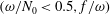 $(\unicode[STIX]{x1D714}/N_{0}<0.5,f/\unicode[STIX]{x1D714})$
as long as there exist mechanisms by which at least a small amount of mode-1 energy is put into modes 2–7. Of significance is the presence of at least one divergence curve for all the modal interactions we consider in figure 6(a). Furthermore, multiple divergence curves occur for a fixed
$(\unicode[STIX]{x1D714}/N_{0}<0.5,f/\unicode[STIX]{x1D714})$
as long as there exist mechanisms by which at least a small amount of mode-1 energy is put into modes 2–7. Of significance is the presence of at least one divergence curve for all the modal interactions we consider in figure 6(a). Furthermore, multiple divergence curves occur for a fixed
 $(m,\,n)$
where
$(m,\,n)$
where
 $m=1$
and
$m=1$
and
 $4\leqslant n\leqslant 7$
. In fact,
$4\leqslant n\leqslant 7$
. In fact,
 $(1,7)$
interaction corresponds to four different divergence curves in figure 6(a). We recall that a given
$(1,7)$
interaction corresponds to four different divergence curves in figure 6(a). We recall that a given
 $(m,\,n)$
interaction can result in at most one divergence curve on the
$(m,\,n)$
interaction can result in at most one divergence curve on the
 $(\unicode[STIX]{x1D714}/N_{0},f/\unicode[STIX]{x1D714})$
plane for a uniform stratification.
$(\unicode[STIX]{x1D714}/N_{0},f/\unicode[STIX]{x1D714})$
plane for a uniform stratification.
For
 $N_{max}=4N_{0}$
(figure 6
b), there is again a large number of divergence curves, now spread over the entire
$N_{max}=4N_{0}$
(figure 6
b), there is again a large number of divergence curves, now spread over the entire
 $(\unicode[STIX]{x1D714}/N_{0},f/\unicode[STIX]{x1D714})$
plane, for
$(\unicode[STIX]{x1D714}/N_{0},f/\unicode[STIX]{x1D714})$
plane, for
 $m=1$
and
$m=1$
and
 $2\leqslant n\leqslant 7$
, with some of them being horizontal at large
$2\leqslant n\leqslant 7$
, with some of them being horizontal at large
 $f/\unicode[STIX]{x1D714}$
even for small
$f/\unicode[STIX]{x1D714}$
even for small
 $n$
. For the strongest-pycnocline case of
$n$
. For the strongest-pycnocline case of
 $N_{max}=10N_{0}$
(figure 6
c), low-mode interactions
$N_{max}=10N_{0}$
(figure 6
c), low-mode interactions
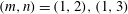 $(m,\,n)=(1,2),(1,3)$
result in near-horizontal divergence curves at
$(m,\,n)=(1,2),(1,3)$
result in near-horizontal divergence curves at
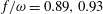 $f/\unicode[STIX]{x1D714}=0.89,0.93$
, respectively. The interaction of mode-1 with higher modes (
$f/\unicode[STIX]{x1D714}=0.89,0.93$
, respectively. The interaction of mode-1 with higher modes (
 $n=4{-}7$
) again leads to more divergence curves that span a wide range of
$n=4{-}7$
) again leads to more divergence curves that span a wide range of
 $\unicode[STIX]{x1D714}/N_{0}$
and
$\unicode[STIX]{x1D714}/N_{0}$
and
 $f/\unicode[STIX]{x1D714}$
. In summary, RTIs are likely to occur in the ocean as a result of interaction between mode-1 and the higher modes generated by topographic scattering of mode-1. An interesting observation from figure 6 is the contrasting effect of increasing
$f/\unicode[STIX]{x1D714}$
. In summary, RTIs are likely to occur in the ocean as a result of interaction between mode-1 and the higher modes generated by topographic scattering of mode-1. An interesting observation from figure 6 is the contrasting effect of increasing
 $N_{max}$
on the number of divergence curves in the small-
$N_{max}$
on the number of divergence curves in the small-
 $f/\unicode[STIX]{x1D714}$
region of the
$f/\unicode[STIX]{x1D714}$
region of the
 $(\unicode[STIX]{x1D714}/N_{0},f/\unicode[STIX]{x1D714})$
plane. For
$(\unicode[STIX]{x1D714}/N_{0},f/\unicode[STIX]{x1D714})$
plane. For
 $\unicode[STIX]{x1D714}/N_{0}<0.5$
, for which the higher harmonic wave at
$\unicode[STIX]{x1D714}/N_{0}<0.5$
, for which the higher harmonic wave at
 $2\unicode[STIX]{x1D714}$
is propagating throughout the ocean depth, the number of divergence curves passing through the
$2\unicode[STIX]{x1D714}$
is propagating throughout the ocean depth, the number of divergence curves passing through the
 $f/\unicode[STIX]{x1D714}=0$
line noticeably decreases with an increase in
$f/\unicode[STIX]{x1D714}=0$
line noticeably decreases with an increase in
 $N_{max}$
. In contrast, for
$N_{max}$
. In contrast, for
 $\unicode[STIX]{x1D714}/N_{0}>0.5$
, for which internal wave propagation at
$\unicode[STIX]{x1D714}/N_{0}>0.5$
, for which internal wave propagation at
 $2\unicode[STIX]{x1D714}$
is restricted to the pycnocline region, the number of divergence curves passing through
$2\unicode[STIX]{x1D714}$
is restricted to the pycnocline region, the number of divergence curves passing through
 $f/\unicode[STIX]{x1D714}=0$
increases with an increase in
$f/\unicode[STIX]{x1D714}=0$
increases with an increase in
 $N_{max}$
. In summary, figure 6 suggests that a significantly larger number of resonant mode interactions occur in a non-uniform stratification compared to a uniform stratification.
$N_{max}$
. In summary, figure 6 suggests that a significantly larger number of resonant mode interactions occur in a non-uniform stratification compared to a uniform stratification.
It may be potentially interesting to include primary waves that propagate in the negative
 $x$
-direction to model interaction between incident and reflected waves at topographic sites. The dissipation of high-mode internal tides close to the generation sites can also be initiated by a nonlinear transfer of energy to higher frequencies and smaller length scales that result from modal interactions at the semidiurnal frequency. Finally, the existence of RTI arising from modal interactions raises questions about the validity of linear models of generation and scattering that assume a range of vertical modes at a fixed frequency in the wave field.
$x$
-direction to model interaction between incident and reflected waves at topographic sites. The dissipation of high-mode internal tides close to the generation sites can also be initiated by a nonlinear transfer of energy to higher frequencies and smaller length scales that result from modal interactions at the semidiurnal frequency. Finally, the existence of RTI arising from modal interactions raises questions about the validity of linear models of generation and scattering that assume a range of vertical modes at a fixed frequency in the wave field.
4.2 Internal wave beam incident on a pycnocline
The generation of mean flow and superharmonics shown in this paper is strikingly similar to the nonlinear effects that result from colliding plane waves or wave beams, a prevalent occurrence when an internal wave beam interacts with either a solid boundary (Peacock & Tabaei Reference Peacock and Tabaei2005) or a free-slip surface (Zhou & Diamessis Reference Zhou and Diamessis2013) or with the ocean pycnocline (Grisouard, Staquet & Gerkema Reference Grisouard, Staquet and Gerkema2011; Mercier et al. Reference Mercier, Mathur, Gostiaux, Gerkema, Magalhaes, Da Silva and Dauxois2012). It may therefore be worthwhile to model these occurrences as nonlinear interaction between modes rather than as localized interaction between colliding plane waves or wave beams. For example, the qualitative differences in harmonic wave generation observed for various pycnoclines (Diamessis et al. Reference Diamessis, Wunsch, Delwiche and Richter2014) could be explained using a modal representation of the incident wave beam, which we now proceed to elucidate further.

Figure 7. (a) Schematic depicting the flow studied by Diamessis et al. (Reference Diamessis, Wunsch, Delwiche and Richter2014) and discussed in § 4.2. An upward-propagating wave beam of dominant horizontal wavelength
 $\unicode[STIX]{x1D706}_{x}$
in a stratification
$\unicode[STIX]{x1D706}_{x}$
in a stratification
 $N_{0}$
is incident on a pycnocline of thickness
$N_{0}$
is incident on a pycnocline of thickness
 $h$
and maximum stratification
$h$
and maximum stratification
 $N_{max}$
. (b) Energy flux fraction
$N_{max}$
. (b) Energy flux fraction
 $E_{m}$
in mode-
$E_{m}$
in mode-
 $m$
for various pycnocline strengths (
$m$
for various pycnocline strengths (
 $N_{max}=(1.5,3,4,6,8,10)N_{0}$
from left to right) and a fixed pycnocline thickness given by
$N_{max}=(1.5,3,4,6,8,10)N_{0}$
from left to right) and a fixed pycnocline thickness given by
 $h/\unicode[STIX]{x1D706}_{x}=1$
.
$h/\unicode[STIX]{x1D706}_{x}=1$
.
As shown in figure 7, Diamessis et al. (Reference Diamessis, Wunsch, Delwiche and Richter2014) numerically studied the dynamics of an upward-propagating internal wave beam of dominant wavelength
 $\unicode[STIX]{x1D706}_{x}$
in the constant deep ocean stratification
$\unicode[STIX]{x1D706}_{x}$
in the constant deep ocean stratification
 $N_{0}$
incident on a pycnocline whose thickness is
$N_{0}$
incident on a pycnocline whose thickness is
 $h$
and where the maximum stratification is denoted by
$h$
and where the maximum stratification is denoted by
 $N_{max}$
. The stratification profile and the incident wave beam profile are both described in Diamessis et al. (Reference Diamessis, Wunsch, Delwiche and Richter2014). The incident wave frequency was specified as
$N_{max}$
. The stratification profile and the incident wave beam profile are both described in Diamessis et al. (Reference Diamessis, Wunsch, Delwiche and Richter2014). The incident wave frequency was specified as
 $\unicode[STIX]{x1D714}=N_{0}/\sqrt{2}$
corresponding to a 45
$\unicode[STIX]{x1D714}=N_{0}/\sqrt{2}$
corresponding to a 45
 $^{\circ }$
wave beam, which corresponds to the first higher harmonic
$^{\circ }$
wave beam, which corresponds to the first higher harmonic
 $2\unicode[STIX]{x1D714}$
being evanescent in the deep ocean. It was shown that higher harmonics were invariably generated as a result of the interaction between the incident wave beam and the pycnocline, with the amplitude and number of higher harmonics increasing with
$2\unicode[STIX]{x1D714}$
being evanescent in the deep ocean. It was shown that higher harmonics were invariably generated as a result of the interaction between the incident wave beam and the pycnocline, with the amplitude and number of higher harmonics increasing with
 $N_{max}/N_{0}$
for a given normalized pycnocline thickness
$N_{max}/N_{0}$
for a given normalized pycnocline thickness
 $h/\unicode[STIX]{x1D706}_{x}$
.
$h/\unicode[STIX]{x1D706}_{x}$
.
For a thin pycnocline, i.e.
 $h/\unicode[STIX]{x1D706}_{x}=0.1$
, it was shown by Diamessis et al. (Reference Diamessis, Wunsch, Delwiche and Richter2014) that the amplitudes of the higher harmonics were largest when their frequencies and wavenumbers satisfy the interfacial wave dispersion relation. They then proceed to construct a theoretical model that considers a plane internal wave incident on a sharp interface across which there is a density jump, with no boundaries either below or above the sharp interface. Interfacial waves are relevant only in the limit of extremely thin pycnoclines and with the primary wave frequency
$h/\unicode[STIX]{x1D706}_{x}=0.1$
, it was shown by Diamessis et al. (Reference Diamessis, Wunsch, Delwiche and Richter2014) that the amplitudes of the higher harmonics were largest when their frequencies and wavenumbers satisfy the interfacial wave dispersion relation. They then proceed to construct a theoretical model that considers a plane internal wave incident on a sharp interface across which there is a density jump, with no boundaries either below or above the sharp interface. Interfacial waves are relevant only in the limit of extremely thin pycnoclines and with the primary wave frequency
 $\unicode[STIX]{x1D714}$
satisfying
$\unicode[STIX]{x1D714}$
satisfying
 $2\unicode[STIX]{x1D714}>N_{0}$
, thus rendering the higher harmonics evanescent in the deep ocean. In our theoretical framework, the influence of the boundaries both below and above the pycnocline is completely accounted for, and there are no assumptions about either the pycnocline thickness or the primary wave frequency. In the limit of
$2\unicode[STIX]{x1D714}>N_{0}$
, thus rendering the higher harmonics evanescent in the deep ocean. In our theoretical framework, the influence of the boundaries both below and above the pycnocline is completely accounted for, and there are no assumptions about either the pycnocline thickness or the primary wave frequency. In the limit of
 $h/\unicode[STIX]{x1D706}_{x}\ll 1$
,
$h/\unicode[STIX]{x1D706}_{x}\ll 1$
,
 $2\unicode[STIX]{x1D714}>N_{0}$
and the ocean boundaries being far from the pycnocline, the existence of a resonant triad with two modes at frequency
$2\unicode[STIX]{x1D714}>N_{0}$
and the ocean boundaries being far from the pycnocline, the existence of a resonant triad with two modes at frequency
 $\unicode[STIX]{x1D714}$
and the third at frequency
$\unicode[STIX]{x1D714}$
and the third at frequency
 $2\unicode[STIX]{x1D714}$
is equivalent to the requirement of the higher harmonics having to satisfy the interfacial wave dispersion relation. Furthermore, the presence of boundaries above and below the thin pycnocline restricts the number of interfacial mode wavenumbers to be countably infinite, as opposed to the possibility of a continuous range of wavenumbers when there are no boundaries. In summary, the thin-pycnocline results of Diamessis et al. (Reference Diamessis, Wunsch, Delwiche and Richter2014) reaffirm our conclusion that the existence of a resonant triad results in the amplification of the higher harmonics.
$2\unicode[STIX]{x1D714}$
is equivalent to the requirement of the higher harmonics having to satisfy the interfacial wave dispersion relation. Furthermore, the presence of boundaries above and below the thin pycnocline restricts the number of interfacial mode wavenumbers to be countably infinite, as opposed to the possibility of a continuous range of wavenumbers when there are no boundaries. In summary, the thin-pycnocline results of Diamessis et al. (Reference Diamessis, Wunsch, Delwiche and Richter2014) reaffirm our conclusion that the existence of a resonant triad results in the amplification of the higher harmonics.

Figure 8. The product
 $E_{m}E_{n}$
shown in colour as a function of
$E_{m}E_{n}$
shown in colour as a function of
 $m$
and
$m$
and
 $n$
for the incident wave beam shown in figure 7 and for (a)
$n$
for the incident wave beam shown in figure 7 and for (a)
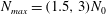 $N_{max}=(1.5,3)N_{0}$
, (b)
$N_{max}=(1.5,3)N_{0}$
, (b)
 $N_{max}=(4,6)N_{0}$
and (c)
$N_{max}=(4,6)N_{0}$
and (c)
 $N_{max}=(8,10)N_{0}$
. In each plot, the small and large
$N_{max}=(8,10)N_{0}$
. In each plot, the small and large
 $N_{max}$
cases are shown at the top left and bottom right, respectively. The pink (top left) and black (bottom right) points mark the
$N_{max}$
cases are shown at the top left and bottom right, respectively. The pink (top left) and black (bottom right) points mark the
 $(m,\,n)$
combinations for which
$(m,\,n)$
combinations for which
 $k^{d}=|(k_{m}+k_{n}-k_{q}^{2\unicode[STIX]{x1D714}})|/k_{q}^{2\unicode[STIX]{x1D714}}$
is less than 0.01 for the corresponding stratification, indicating that the
$k^{d}=|(k_{m}+k_{n}-k_{q}^{2\unicode[STIX]{x1D714}})|/k_{q}^{2\unicode[STIX]{x1D714}}$
is less than 0.01 for the corresponding stratification, indicating that the
 $(m,\,n)$
pair of modes at frequency
$(m,\,n)$
pair of modes at frequency
 $\unicode[STIX]{x1D714}$
could form a resonant triad with mode-
$\unicode[STIX]{x1D714}$
could form a resonant triad with mode-
 $q$
at frequency
$q$
at frequency
 $2\unicode[STIX]{x1D714}$
.
$2\unicode[STIX]{x1D714}$
.
For a thick pycnocline, i.e.
 $h/\unicode[STIX]{x1D706}_{x}=1$
, Diamessis et al. (Reference Diamessis, Wunsch, Delwiche and Richter2014) observe harmonic generation at multiple locations in the pycnocline, thus resulting in a complex flow pattern. Here, we present the results of our analysis for six different values of
$h/\unicode[STIX]{x1D706}_{x}=1$
, Diamessis et al. (Reference Diamessis, Wunsch, Delwiche and Richter2014) observe harmonic generation at multiple locations in the pycnocline, thus resulting in a complex flow pattern. Here, we present the results of our analysis for six different values of
 $N_{max}/N_{0}$
with a fixed normalized pycnocline thickness of
$N_{max}/N_{0}$
with a fixed normalized pycnocline thickness of
 $h/\unicode[STIX]{x1D706}_{x}=1$
. In figure 7(b), we show the fractional distribution of energy fluxes in various modes corresponding to the incident wave beam in figure 7(a). The energy flux distribution moves rightwards to higher modes as
$h/\unicode[STIX]{x1D706}_{x}=1$
. In figure 7(b), we show the fractional distribution of energy fluxes in various modes corresponding to the incident wave beam in figure 7(a). The energy flux distribution moves rightwards to higher modes as
 $N_{max}/N_{0}$
is increased from 1.5 to 10. For each of the six
$N_{max}/N_{0}$
is increased from 1.5 to 10. For each of the six
 $N_{max}/N_{0}$
values, we explore the existence of resonant triads containing a pair of modes
$N_{max}/N_{0}$
values, we explore the existence of resonant triads containing a pair of modes
 $(m,\,n)$
(with non-negligible
$(m,\,n)$
(with non-negligible
 $E_{m}$
and
$E_{m}$
and
 $E_{n}$
) at the primary wave frequency
$E_{n}$
) at the primary wave frequency
 $\unicode[STIX]{x1D714}$
. The existence of a resonant triad is established by verifying if the condition
$\unicode[STIX]{x1D714}$
. The existence of a resonant triad is established by verifying if the condition
 $k^{d}=|(k_{m}+k_{n}-k_{q}^{2\unicode[STIX]{x1D714}})|/k_{q}^{2\unicode[STIX]{x1D714}}=0$
is satisfied within a specified limit. Here,
$k^{d}=|(k_{m}+k_{n}-k_{q}^{2\unicode[STIX]{x1D714}})|/k_{q}^{2\unicode[STIX]{x1D714}}=0$
is satisfied within a specified limit. Here,
 $q$
is calculated as
$q$
is calculated as
 $q=n_{z}+1$
, where
$q=n_{z}+1$
, where
 $n_{z}$
is the number of zeros in
$n_{z}$
is the number of zeros in
 $h_{mn}(z)$
. We recall from figure 3 and § 3.4 that regions of small values of
$h_{mn}(z)$
. We recall from figure 3 and § 3.4 that regions of small values of
 $k^{d}$
indeed capture the regions in the neighbourhood of divergence curves/triadic resonance.
$k^{d}$
indeed capture the regions in the neighbourhood of divergence curves/triadic resonance.
In figure 8(a–c), we show the distribution of
 $E_{m}E_{n}$
as a function of mode numbers
$E_{m}E_{n}$
as a function of mode numbers
 $m$
and
$m$
and
 $n$
for six different values of
$n$
for six different values of
 $N_{max}/N_{0}$
and a fixed value for the normalized pycnocline thickness
$N_{max}/N_{0}$
and a fixed value for the normalized pycnocline thickness
 $h/\unicode[STIX]{x1D706}_{x}=1$
(thick pycnocline based on the terminology of Diamessis et al. (Reference Diamessis, Wunsch, Delwiche and Richter2014)). In each of figure 8(a–c), the distributions for two values of
$h/\unicode[STIX]{x1D706}_{x}=1$
(thick pycnocline based on the terminology of Diamessis et al. (Reference Diamessis, Wunsch, Delwiche and Richter2014)). In each of figure 8(a–c), the distributions for two values of
 $N_{max}/N_{0}$
are shown as indicated within each figure. As shown in (2.16), the magnitude of
$N_{max}/N_{0}$
are shown as indicated within each figure. As shown in (2.16), the magnitude of
 $h_{mn}$
is directly proportional to
$h_{mn}$
is directly proportional to
 $\sqrt{E_{m}E_{n}}$
; thus, it is relevant to look for only those resonant triads which contain modes
$\sqrt{E_{m}E_{n}}$
; thus, it is relevant to look for only those resonant triads which contain modes
 $m$
and
$m$
and
 $n$
(at frequency
$n$
(at frequency
 $\unicode[STIX]{x1D714}$
) for which
$\unicode[STIX]{x1D714}$
) for which
 $\sqrt{E_{m}E_{n}}$
is non-negligible. Also shown as individual points (coloured pink and black) in figure 8 are the
$\sqrt{E_{m}E_{n}}$
is non-negligible. Also shown as individual points (coloured pink and black) in figure 8 are the
 $(m,\,n)$
combinations for which
$(m,\,n)$
combinations for which
 $|k^{d}|$
is less than 0.01 for the corresponding
$|k^{d}|$
is less than 0.01 for the corresponding
 $N_{max}/N_{0}$
. For
$N_{max}/N_{0}$
. For
 $N_{max}/N_{0}=1.5$
(top left of figure 8
a), the absence of any pink points indicates that there are no resonant triads containing modes
$N_{max}/N_{0}=1.5$
(top left of figure 8
a), the absence of any pink points indicates that there are no resonant triads containing modes
 $m$
and
$m$
and
 $n$
at frequency
$n$
at frequency
 $\unicode[STIX]{x1D714}$
with non-negligible
$\unicode[STIX]{x1D714}$
with non-negligible
 $E_{m}$
and
$E_{m}$
and
 $E_{n}$
. For
$E_{n}$
. For
 $N_{max}/N_{0}=3$
(bottom right of figure 8
a),
$N_{max}/N_{0}=3$
(bottom right of figure 8
a),
 $k^{d}\ll 1$
(black points) occurs at
$k^{d}\ll 1$
(black points) occurs at
 $(m,\,n)=(10,10)$
(self-interaction) and
$(m,\,n)=(10,10)$
(self-interaction) and
 $(m,\,n)=(25,23)$
, both of which imply the existence of resonant triads. The resonant triad containing
$(m,\,n)=(25,23)$
, both of which imply the existence of resonant triads. The resonant triad containing
 $(m,\,n)=(25,23)$
is potentially significant as the value of
$(m,\,n)=(25,23)$
is potentially significant as the value of
 $E_{m}E_{n}$
is appreciable, as indicated by the background colour. It is therefore expected that the higher harmonic waves are stronger for the case of
$E_{m}E_{n}$
is appreciable, as indicated by the background colour. It is therefore expected that the higher harmonic waves are stronger for the case of
 $N_{max}/N_{0}=3$
in comparison to
$N_{max}/N_{0}=3$
in comparison to
 $N_{max}/N_{0}=1.5$
. As we increase
$N_{max}/N_{0}=1.5$
. As we increase
 $N_{max}/N_{0}$
further (figure 8
b,c), we observe an increase in the number of resonant triads within the region of non-negligible
$N_{max}/N_{0}$
further (figure 8
b,c), we observe an increase in the number of resonant triads within the region of non-negligible
 $E_{m}E_{n}$
and therefore conclude that the amplitude of higher harmonics is likely to be larger for larger
$E_{m}E_{n}$
and therefore conclude that the amplitude of higher harmonics is likely to be larger for larger
 $N_{max}/N_{0}$
for a fixed value of
$N_{max}/N_{0}$
for a fixed value of
 $h/\unicode[STIX]{x1D706}_{x}=1$
. This offers an explanation for one of the main observations of Diamessis et al. (Reference Diamessis, Wunsch, Delwiche and Richter2014), namely that the number and amplitude of higher harmonics increase with a stratification parameter defined as
$h/\unicode[STIX]{x1D706}_{x}=1$
. This offers an explanation for one of the main observations of Diamessis et al. (Reference Diamessis, Wunsch, Delwiche and Richter2014), namely that the number and amplitude of higher harmonics increase with a stratification parameter defined as
 $\unicode[STIX]{x1D6FE}=(N_{max}/N_{0})/(h/\unicode[STIX]{x1D706}_{x})$
. The precise number, amplitude and spatial pattern of higher harmonics would, however, require calculations of the energy transfer rates within the identified resonant triads, and also a consideration of interactions that occur at higher frequencies. As a follow-up study, it would be intriguing to investigate the relation between stratification profiles that are conducive to solitary wave generation (Gerkema Reference Gerkema2001) and those that correspond to the existence of a large number of resonant triads that contain the modes present in the incident wave beam.
$\unicode[STIX]{x1D6FE}=(N_{max}/N_{0})/(h/\unicode[STIX]{x1D706}_{x})$
. The precise number, amplitude and spatial pattern of higher harmonics would, however, require calculations of the energy transfer rates within the identified resonant triads, and also a consideration of interactions that occur at higher frequencies. As a follow-up study, it would be intriguing to investigate the relation between stratification profiles that are conducive to solitary wave generation (Gerkema Reference Gerkema2001) and those that correspond to the existence of a large number of resonant triads that contain the modes present in the incident wave beam.
5 Conclusions
In this paper, we have shown the existence of pure resonant triads in finite-depth non-uniform stratifications with background rotation. The weakly nonlinear solution corresponding to interaction between modes
 $m$
and
$m$
and
 $n$
in the linear solution comprises two different terms, one at frequency
$n$
in the linear solution comprises two different terms, one at frequency
 $2\unicode[STIX]{x1D714}$
(horizontal wavenumber
$2\unicode[STIX]{x1D714}$
(horizontal wavenumber
 $k_{m}+k_{n}$
and vertical profile
$k_{m}+k_{n}$
and vertical profile
 $\bar{h}_{mn}(z)$
) and the other being time independent. The amplitude of the superharmonic term diverges if a resonance condition in the governing equation for
$\bar{h}_{mn}(z)$
) and the other being time independent. The amplitude of the superharmonic term diverges if a resonance condition in the governing equation for
 $\bar{h}_{mn}(z)$
is met. The resonance condition is also interpreted as the existence of a resonant triad comprising modes
$\bar{h}_{mn}(z)$
is met. The resonance condition is also interpreted as the existence of a resonant triad comprising modes
 $m$
and
$m$
and
 $n$
at frequency
$n$
at frequency
 $\unicode[STIX]{x1D714}$
and the higher harmonic internal wave at frequency
$\unicode[STIX]{x1D714}$
and the higher harmonic internal wave at frequency
 $2\unicode[STIX]{x1D714}$
. The mode number
$2\unicode[STIX]{x1D714}$
. The mode number
 $q$
of the higher harmonic wave is
$q$
of the higher harmonic wave is
 $q=|m-n|$
for a uniform stratification, but seems to take some value less than
$q=|m-n|$
for a uniform stratification, but seems to take some value less than
 $\max (m,\,n)$
for a non-uniform stratification with a pycnocline.
$\max (m,\,n)$
for a non-uniform stratification with a pycnocline.
For a given modal pair
 $(m,\,n)$
, the resonance condition is satisfied along specific divergence curves on the
$(m,\,n)$
, the resonance condition is satisfied along specific divergence curves on the
 $(\unicode[STIX]{x1D714}/N_{0},f/\unicode[STIX]{x1D714})$
plane in both uniform stratifications and ocean-like non-uniform stratifications. In uniform stratifications, a unique divergence curve exists for a given
$(\unicode[STIX]{x1D714}/N_{0},f/\unicode[STIX]{x1D714})$
plane in both uniform stratifications and ocean-like non-uniform stratifications. In uniform stratifications, a unique divergence curve exists for a given
 $(m,\,n)$
that satisfies
$(m,\,n)$
that satisfies
 $(m/3)<n<3m$
. For the case of
$(m/3)<n<3m$
. For the case of
 $m/n$
close to unity, the divergence curves tend to become horizontal and accumulate close to
$m/n$
close to unity, the divergence curves tend to become horizontal and accumulate close to
 $f/\unicode[STIX]{x1D714}\approx 1$
. In non-uniform stratifications with a pycnocline, divergence curves occur for several more modal interactions than those for the uniform stratification; in fact, divergence curves occur for all
$f/\unicode[STIX]{x1D714}\approx 1$
. In non-uniform stratifications with a pycnocline, divergence curves occur for several more modal interactions than those for the uniform stratification; in fact, divergence curves occur for all
 $(m,\,n\neq m)$
we considered: (
$(m,\,n\neq m)$
we considered: (
 $m=1,2\leqslant n\leqslant 7$
), (
$m=1,2\leqslant n\leqslant 7$
), (
 $m=2,3\leqslant n\leqslant 5$
) and self-interactions too. Furthermore, multiple divergence curves occur for many
$m=2,3\leqslant n\leqslant 5$
) and self-interactions too. Furthermore, multiple divergence curves occur for many
 $(m,\,n)$
in non-uniform stratifications with a pycnocline, a significant consequence of which is an increase in the extent of the region on the
$(m,\,n)$
in non-uniform stratifications with a pycnocline, a significant consequence of which is an increase in the extent of the region on the
 $(\unicode[STIX]{x1D714}/N_{0},f/\unicode[STIX]{x1D714})$
plane where the higher harmonic solutions are of a large magnitude. For sufficiently strong pycnoclines, we observe the occurrence of near-horizontal divergence curves near
$(\unicode[STIX]{x1D714}/N_{0},f/\unicode[STIX]{x1D714})$
plane where the higher harmonic solutions are of a large magnitude. For sufficiently strong pycnoclines, we observe the occurrence of near-horizontal divergence curves near
 $f/\unicode[STIX]{x1D714}\approx 1$
even for values of
$f/\unicode[STIX]{x1D714}\approx 1$
even for values of
 $m/n$
far from unity, potentially a significant factor for understanding nonlinear effects in near-inertial waves. Remarkably, resonance occurs even for self-interaction (
$m/n$
far from unity, potentially a significant factor for understanding nonlinear effects in near-inertial waves. Remarkably, resonance occurs even for self-interaction (
 $m=n$
) in a non-uniform stratification, thus rendering the corresponding distinct modes at frequency
$m=n$
) in a non-uniform stratification, thus rendering the corresponding distinct modes at frequency
 $\unicode[STIX]{x1D714}$
unstable irrespective of their amplitude.
$\unicode[STIX]{x1D714}$
unstable irrespective of their amplitude.
The divergence of the higher harmonic weakly nonlinear solution was shown to occur upon satisfying two different criteria: (i)
 $k_{m}+k_{n}=k_{s}^{2\unicode[STIX]{x1D714}}$
, where
$k_{m}+k_{n}=k_{s}^{2\unicode[STIX]{x1D714}}$
, where
 $k_{s}^{2\unicode[STIX]{x1D714}}$
is the horizontal wavenumber of some mode-
$k_{s}^{2\unicode[STIX]{x1D714}}$
is the horizontal wavenumber of some mode-
 $s$
at frequency
$s$
at frequency
 $2\unicode[STIX]{x1D714}$
, and (ii) the right-hand side
$2\unicode[STIX]{x1D714}$
, and (ii) the right-hand side
 $\bar{C}_{mn}(z)$
of the governing equation (2.18) of
$\bar{C}_{mn}(z)$
of the governing equation (2.18) of
 $\bar{h}_{mn}(z)$
should not be orthogonal to
$\bar{h}_{mn}(z)$
should not be orthogonal to
 $Q_{s}^{2\unicode[STIX]{x1D714}}(z)$
, where
$Q_{s}^{2\unicode[STIX]{x1D714}}(z)$
, where
 $Q_{s}^{2\unicode[STIX]{x1D714}}(z)$
is the vertical structure of mode-
$Q_{s}^{2\unicode[STIX]{x1D714}}(z)$
is the vertical structure of mode-
 $s$
at frequency
$s$
at frequency
 $2\unicode[STIX]{x1D714}$
. Criterion (i) is the same as the horizontal component of the standard triadic resonance criterion
$2\unicode[STIX]{x1D714}$
. Criterion (i) is the same as the horizontal component of the standard triadic resonance criterion
 $\boldsymbol{k}_{1}+\boldsymbol{k}_{2}+\boldsymbol{k}_{3}=0$
. For uniform stratifications, criterion (ii) coincides with the vertical component of
$\boldsymbol{k}_{1}+\boldsymbol{k}_{2}+\boldsymbol{k}_{3}=0$
. For uniform stratifications, criterion (ii) coincides with the vertical component of
 $\boldsymbol{k}_{1}+\boldsymbol{k}_{2}+\boldsymbol{k}_{3}=0$
, and is not necessarily satisfied upon satisfying criterion (i). In fact, there exist non-divergence curves on the
$\boldsymbol{k}_{1}+\boldsymbol{k}_{2}+\boldsymbol{k}_{3}=0$
, and is not necessarily satisfied upon satisfying criterion (i). In fact, there exist non-divergence curves on the
 $(\unicode[STIX]{x1D714}/N_{0},f/\unicode[STIX]{x1D714})$
plane along which criterion (i) but not criterion (ii) is satisfied for a uniform stratification. For non-uniform stratifications with a pycnocline, however, criterion (ii) was always satisfied upon the satisfaction of criterion (i) for all the cases we considered, and hence results in several more divergence curve/triadic resonance interactions than for a uniform stratification.
$(\unicode[STIX]{x1D714}/N_{0},f/\unicode[STIX]{x1D714})$
plane along which criterion (i) but not criterion (ii) is satisfied for a uniform stratification. For non-uniform stratifications with a pycnocline, however, criterion (ii) was always satisfied upon the satisfaction of criterion (i) for all the cases we considered, and hence results in several more divergence curve/triadic resonance interactions than for a uniform stratification.
Two representative oceanic scenarios, namely low-mode internal tide scattering by topography and internal wave beam interaction with the pycnocline, were then discussed. In non-uniform stratifications with a pycnocline, mode-1 interaction with higher modes results in divergence curves over large portions of the
 $(\unicode[STIX]{x1D714}/N_{0},f/\unicode[STIX]{x1D714})$
plane, suggesting that RTIs are likely to occur over small-scale random topography in the ocean. The generation of higher harmonics upon the interaction of an internal wave beam with the pycnocline was then associated with the existence of resonant triads comprising two modes at frequency
$(\unicode[STIX]{x1D714}/N_{0},f/\unicode[STIX]{x1D714})$
plane, suggesting that RTIs are likely to occur over small-scale random topography in the ocean. The generation of higher harmonics upon the interaction of an internal wave beam with the pycnocline was then associated with the existence of resonant triads comprising two modes at frequency
 $\unicode[STIX]{x1D714}$
contained within the incident wave beam. Consistent with the numerical study of Diamessis et al. (Reference Diamessis, Wunsch, Delwiche and Richter2014), we were able to show that the number of resonant triads that result from interaction between the modes contained in a given incident wave beam increases with the maximum stratification in the pycnocline whose thickness is fixed.
$\unicode[STIX]{x1D714}$
contained within the incident wave beam. Consistent with the numerical study of Diamessis et al. (Reference Diamessis, Wunsch, Delwiche and Richter2014), we were able to show that the number of resonant triads that result from interaction between the modes contained in a given incident wave beam increases with the maximum stratification in the pycnocline whose thickness is fixed.
The most significant contribution of our study is to demonstrate the existence of pure resonant triads in finite-depth non-uniform stratifications when the interaction between modes
 $m$
and
$m$
and
 $n$
is considered. The condition for resonant triad interaction involving modes
$n$
is considered. The condition for resonant triad interaction involving modes
 $m$
and
$m$
and
 $n$
at frequency
$n$
at frequency
 $\unicode[STIX]{x1D714}$
in both uniform and non-uniform stratifications is given by
$\unicode[STIX]{x1D714}$
in both uniform and non-uniform stratifications is given by
 $k^{d}=k_{m}^{\unicode[STIX]{x1D714}}+k_{n}^{\unicode[STIX]{x1D714}}-k_{q}^{2\unicode[STIX]{x1D714}}=0$
, where the notation
$k^{d}=k_{m}^{\unicode[STIX]{x1D714}}+k_{n}^{\unicode[STIX]{x1D714}}-k_{q}^{2\unicode[STIX]{x1D714}}=0$
, where the notation
 $k_{p}^{\unicode[STIX]{x1D6FA}}$
stands for the horizontal wavenumber of mode-
$k_{p}^{\unicode[STIX]{x1D6FA}}$
stands for the horizontal wavenumber of mode-
 $p$
at frequency
$p$
at frequency
 $\unicode[STIX]{x1D6FA}$
. Here,
$\unicode[STIX]{x1D6FA}$
. Here,
 $q$
is given by
$q$
is given by
 $q=n_{z}+1$
, where
$q=n_{z}+1$
, where
 $n_{z}$
is the number of zeros of the particular solution of the vertical structure
$n_{z}$
is the number of zeros of the particular solution of the vertical structure
 $\bar{h}_{mn}(z)$
of the weakly nonlinear higher harmonic solution when a primary wave field containing modes
$\bar{h}_{mn}(z)$
of the weakly nonlinear higher harmonic solution when a primary wave field containing modes
 $m$
and
$m$
and
 $n$
at frequency
$n$
at frequency
 $\unicode[STIX]{x1D714}$
is assumed. It is noted that the particular solution of
$\unicode[STIX]{x1D714}$
is assumed. It is noted that the particular solution of
 $\bar{h}_{mn}(z)$
diverges in the event of
$\bar{h}_{mn}(z)$
diverges in the event of
 $k^{d}$
being exactly zero. However,
$k^{d}$
being exactly zero. However,
 $k^{d}=0$
is never exactly achieved in the numerical solutions, allowing us to build a finite-amplitude solution for
$k^{d}=0$
is never exactly achieved in the numerical solutions, allowing us to build a finite-amplitude solution for
 $\bar{h}_{mn}(z)$
and hence calculate
$\bar{h}_{mn}(z)$
and hence calculate
 $n_{z}$
. It is also noteworthy that numerical calculation of
$n_{z}$
. It is also noteworthy that numerical calculation of
 $\bar{h}_{mn}(z)$
, as against adopting the graphical approach given in § 3.4, allows for a direct and efficient identification of triadic resonance/divergence curves on the entire
$\bar{h}_{mn}(z)$
, as against adopting the graphical approach given in § 3.4, allows for a direct and efficient identification of triadic resonance/divergence curves on the entire
 $(\unicode[STIX]{x1D714}/N_{0},f/\unicode[STIX]{x1D714})$
plane. While our calculations were performed for idealized non-uniform stratifications, they can be readily extended to realistic ocean stratification profiles without making any assumptions about the pycnocline or the mixed layer characteristics. Finally, the inclusion of the effects of background rotation allowed us to discover phenomena that are potentially relevant for the dynamics of near-inertial waves.
$(\unicode[STIX]{x1D714}/N_{0},f/\unicode[STIX]{x1D714})$
plane. While our calculations were performed for idealized non-uniform stratifications, they can be readily extended to realistic ocean stratification profiles without making any assumptions about the pycnocline or the mixed layer characteristics. Finally, the inclusion of the effects of background rotation allowed us to discover phenomena that are potentially relevant for the dynamics of near-inertial waves.
The results in this paper could also represent a mechanism by which wind-generated near-inertial oscillations in the upper ocean get dissipated. Our study may help quantify the relative importance of the nonlinear energy transfer from near-inertial oscillations to other frequencies, in comparison to other mechanisms such as downward radiation of near-inertial waves (Young & Jelloul Reference Young and Jelloul1997) and turbulent dissipation (Hebert & Moum Reference Hebert and Moum1994). The tools presented in this paper can also be useful in the theoretical prediction of PSI and its characteristics in individual modes of a non-uniform stratification, a special case of which (primary wave frequency
 ${\approx}$
twice the inertial frequency) was studied by Young et al. (Reference Young, Tsang and Balmforth2008). Our ongoing efforts include a calculation of the amplitude evolution (and hence the growth rates) associated with the resonant triads identified in this paper and subsequent comparisons with direct numerical simulations. Finally, the influence of background shear, viscosity and three-dimensionality could be included to make our model even more relevant for realistic ocean settings.
${\approx}$
twice the inertial frequency) was studied by Young et al. (Reference Young, Tsang and Balmforth2008). Our ongoing efforts include a calculation of the amplitude evolution (and hence the growth rates) associated with the resonant triads identified in this paper and subsequent comparisons with direct numerical simulations. Finally, the influence of background shear, viscosity and three-dimensionality could be included to make our model even more relevant for realistic ocean settings.
Acknowledgements
The authors thank the Ministry of Earth Sciences, Government of India for financial support under the Monsoon Mission grant MM/2014/IND-002. The insightful comments from the three anonymous reviewers are gratefully acknowledged.
Appendix A. Mean flow in the weakly nonlinear solution
As shown in (3.2), the mean flow given by the time-independent term
 $\bar{g}_{mn}(z)$
does not diverge for any values of
$\bar{g}_{mn}(z)$
does not diverge for any values of
 $\unicode[STIX]{x1D714}/N_{0}$
,
$\unicode[STIX]{x1D714}/N_{0}$
,
 $f/\unicode[STIX]{x1D714}$
,
$f/\unicode[STIX]{x1D714}$
,
 $m$
and
$m$
and
 $n$
in a uniform stratification. For a non-uniform stratification with
$n$
in a uniform stratification. For a non-uniform stratification with
 $N_{max}=4N_{0}$
, we plot
$N_{max}=4N_{0}$
, we plot
 $\log _{10}[\bar{g}_{mn}^{max}]$
as a function of
$\log _{10}[\bar{g}_{mn}^{max}]$
as a function of
 $\unicode[STIX]{x1D714}/N_{0}$
and
$\unicode[STIX]{x1D714}/N_{0}$
and
 $f/\unicode[STIX]{x1D714}$
for three different modal pairs:
$f/\unicode[STIX]{x1D714}$
for three different modal pairs:
 $(m,\,n)=(1,2),(2,3),(2,5)$
in figure 9(a–c), respectively. The mean flow again does not diverge anywhere on the
$(m,\,n)=(1,2),(2,3),(2,5)$
in figure 9(a–c), respectively. The mean flow again does not diverge anywhere on the
 $(\unicode[STIX]{x1D714}/N_{0},f/\unicode[STIX]{x1D714})$
plane, with
$(\unicode[STIX]{x1D714}/N_{0},f/\unicode[STIX]{x1D714})$
plane, with
 $\log _{10}[\bar{g}_{mn}^{max}]$
increasing as a function of
$\log _{10}[\bar{g}_{mn}^{max}]$
increasing as a function of
 $\unicode[STIX]{x1D714}/N_{0}$
and
$\unicode[STIX]{x1D714}/N_{0}$
and
 $f/\unicode[STIX]{x1D714}$
in most of the domain. There, however, exists a vertical line close to
$f/\unicode[STIX]{x1D714}$
in most of the domain. There, however, exists a vertical line close to
 $(\unicode[STIX]{x1D714}/N_{0})=0.955$
along which
$(\unicode[STIX]{x1D714}/N_{0})=0.955$
along which
 $\log _{10}[\bar{g}_{mn}^{max}]$
attains a local minimum for
$\log _{10}[\bar{g}_{mn}^{max}]$
attains a local minimum for
 $(m,\,n)=(2,3)$
(figure 9
b). For
$(m,\,n)=(2,3)$
(figure 9
b). For
 $(m,\,n)=(2,5)$
, as shown in figure 9(c), there again exists a local minimum along a vertical line, now occurring at
$(m,\,n)=(2,5)$
, as shown in figure 9(c), there again exists a local minimum along a vertical line, now occurring at
 $\unicode[STIX]{x1D714}/N_{0}\approx 0.93$
. We have furthermore verified via very fine-resolution (in
$\unicode[STIX]{x1D714}/N_{0}\approx 0.93$
. We have furthermore verified via very fine-resolution (in
 $\unicode[STIX]{x1D714}/N_{0}$
) runs in the vicinity of the local maxima (that occur just to the left of the identified local minima) that there is no divergence of the mean flow in these regions of the parameter space.
$\unicode[STIX]{x1D714}/N_{0}$
) runs in the vicinity of the local maxima (that occur just to the left of the identified local minima) that there is no divergence of the mean flow in these regions of the parameter space.

Figure 9.
 $\text{log}_{10}[\bar{g}_{mn}^{max}]$
plotted as a function of
$\text{log}_{10}[\bar{g}_{mn}^{max}]$
plotted as a function of
 $\unicode[STIX]{x1D714}/N_{0}$
and
$\unicode[STIX]{x1D714}/N_{0}$
and
 $f/\unicode[STIX]{x1D714}$
for
$f/\unicode[STIX]{x1D714}$
for
 $(m,\,n)=$
(a)
$(m,\,n)=$
(a)
 $(1,\,2)$
, (b)
$(1,\,2)$
, (b)
 $(2,3)$
and (c)
$(2,3)$
and (c)
 $(2,\,5)$
with
$(2,\,5)$
with
 $N_{max}=4N_{0}$
. The energy fluxes for each plot are fixed at
$N_{max}=4N_{0}$
. The energy fluxes for each plot are fixed at
 $(E_{m},E_{n})=(0.9,0.1)~\text{W}~\text{m}^{-1}$
.
$(E_{m},E_{n})=(0.9,0.1)~\text{W}~\text{m}^{-1}$
.
Appendix B. Self-interactions in uniform stratification
The governing equation (2.18) for
 $\bar{h}_{mn}(z)$
reduces to
$\bar{h}_{mn}(z)$
reduces to
 $$\begin{eqnarray}{\displaystyle \frac{\text{d}^{2}\bar{h}_{mm}}{\text{d}z^{2}}}+(2k_{m})^{2}{\displaystyle \frac{N_{0}^{2}-(2\unicode[STIX]{x1D714})^{2}}{(2\unicode[STIX]{x1D714})^{2}-f^{2}}}\bar{h}_{mm}=0\end{eqnarray}$$
for
 $n=m$
and a uniform stratification
$n=m$
and a uniform stratification
 $N(z)=N_{0}$
. Equation (B 1) is the well-known governing equation (2.12) for linear internal wave modes with horizontal wavenumber
$N(z)=N_{0}$
. Equation (B 1) is the well-known governing equation (2.12) for linear internal wave modes with horizontal wavenumber
 $2k_{m}$
and frequency
$2k_{m}$
and frequency
 $2\unicode[STIX]{x1D714}$
. Therefore, non-zero solutions exist only if the vertical wavenumber
$2\unicode[STIX]{x1D714}$
. Therefore, non-zero solutions exist only if the vertical wavenumber
 $k_{z,2\unicode[STIX]{x1D714}}$
satisfies
$k_{z,2\unicode[STIX]{x1D714}}$
satisfies
 $$\begin{eqnarray}k_{z,2\unicode[STIX]{x1D714}}=2k_{m}\sqrt{{\displaystyle \frac{N_{0}^{2}-(2\unicode[STIX]{x1D714})^{2}}{(2\unicode[STIX]{x1D714})^{2}-f^{2}}}},\end{eqnarray}$$
with
 $k_{z,2\unicode[STIX]{x1D714}}=s\unicode[STIX]{x03C0}/H$
where the mode number
$k_{z,2\unicode[STIX]{x1D714}}=s\unicode[STIX]{x03C0}/H$
where the mode number
 $s$
of the higher harmonic wave is a positive integer;
$s$
of the higher harmonic wave is a positive integer;
 $s$
can now be written in terms of the mode number
$s$
can now be written in terms of the mode number
 $m$
of the primary wave as
$m$
of the primary wave as
 $$\begin{eqnarray}s=2m\sqrt{{\displaystyle \frac{N_{0}^{2}-(2\unicode[STIX]{x1D714})^{2}}{(2\unicode[STIX]{x1D714})^{2}-f^{2}}}}\sqrt{{\displaystyle \frac{\unicode[STIX]{x1D714}^{2}-f^{2}}{N_{0}^{2}-\unicode[STIX]{x1D714}^{2}}}}.\end{eqnarray}$$
Non-zero solutions for
 $\bar{h}_{mm}(z)$
exist for all combinations of
$\bar{h}_{mm}(z)$
exist for all combinations of
 $\unicode[STIX]{x1D714}/N_{0}$
,
$\unicode[STIX]{x1D714}/N_{0}$
,
 $f/\unicode[STIX]{x1D714}$
and
$f/\unicode[STIX]{x1D714}$
and
 $m$
that give an integer solution for
$m$
that give an integer solution for
 $s$
in (B 3). In the range
$s$
in (B 3). In the range
 $0<(\unicode[STIX]{x1D714}/N_{0})<0.5$
and
$0<(\unicode[STIX]{x1D714}/N_{0})<0.5$
and
 $0<f/\unicode[STIX]{x1D714}<1$
,
$0<f/\unicode[STIX]{x1D714}<1$
,
 $s$
can take any integer value in the range
$s$
can take any integer value in the range
 $1\leqslant s<m$
; each of these possible values of
$1\leqslant s<m$
; each of these possible values of
 $s$
occur along specific curves on the
$s$
occur along specific curves on the
 $(\unicode[STIX]{x1D714}/N_{0},f/\unicode[STIX]{x1D714})$
plane.
$(\unicode[STIX]{x1D714}/N_{0},f/\unicode[STIX]{x1D714})$
plane.
Appendix C. High-mode interactions in uniform stratification
Here, we plot (3.5) on the
 $(\unicode[STIX]{x1D714}/N_{0},f/\unicode[STIX]{x1D714})$
plane for all possible values of
$(\unicode[STIX]{x1D714}/N_{0},f/\unicode[STIX]{x1D714})$
plane for all possible values of
 $m/n$
that can result in the existence of resonant triads containing modes
$m/n$
that can result in the existence of resonant triads containing modes
 $m$
and
$m$
and
 $n$
at frequency
$n$
at frequency
 $\unicode[STIX]{x1D714}$
. Equation (3.5) is rewritten as
$\unicode[STIX]{x1D714}$
. Equation (3.5) is rewritten as
 $$\begin{eqnarray}{\displaystyle \frac{\unicode[STIX]{x1D714}^{2}}{N_{0}^{2}}}={\displaystyle \frac{(m/n+1)^{2}-(m/n-1)^{2}(4-f^{2}/\unicode[STIX]{x1D714}^{2})/(1-f^{2}/\unicode[STIX]{x1D714}^{2})}{4(m/n+1)^{2}-(m/n-1)^{2}(4-f^{2}/\unicode[STIX]{x1D714}^{2})/(1-f^{2}/\unicode[STIX]{x1D714}^{2})}}.\end{eqnarray}$$
As shown by condition (3.6) in § 3.1,
 $m/n$
has to be in the range
$m/n$
has to be in the range
 $(1/3)<(m/n)<3$
for any divergence curve/resonant triad to exist on the
$(1/3)<(m/n)<3$
for any divergence curve/resonant triad to exist on the
 $(\unicode[STIX]{x1D714}/N_{0},f/\unicode[STIX]{x1D714})$
plane. Since equation (C 1) is invariant with an interchange of
$(\unicode[STIX]{x1D714}/N_{0},f/\unicode[STIX]{x1D714})$
plane. Since equation (C 1) is invariant with an interchange of
 $m$
and
$m$
and
 $n$
, we proceed to plot the divergence curves as
$n$
, we proceed to plot the divergence curves as
 $f/\unicode[STIX]{x1D714}$
versus
$f/\unicode[STIX]{x1D714}$
versus
 $\unicode[STIX]{x1D714}/N_{0}$
for the smaller range of
$\unicode[STIX]{x1D714}/N_{0}$
for the smaller range of
 $1<(m/n)<3$
.
$1<(m/n)<3$
.

Figure 10.
 $f/\unicode[STIX]{x1D714}$
plotted as a function of
$f/\unicode[STIX]{x1D714}$
plotted as a function of
 $\unicode[STIX]{x1D714}/N_{0}$
as given by (C 1) for resonant triads containing modes
$\unicode[STIX]{x1D714}/N_{0}$
as given by (C 1) for resonant triads containing modes
 $m$
and
$m$
and
 $n$
to exist in a uniform stratification. The ten different curves correspond to increasing (in the direction of the arrow) equispaced values of
$n$
to exist in a uniform stratification. The ten different curves correspond to increasing (in the direction of the arrow) equispaced values of
 $m/n$
in the range
$m/n$
in the range
 $1.1\leqslant (m/n)\leqslant 2.9$
.
$1.1\leqslant (m/n)\leqslant 2.9$
.
Figure 10 shows that for
 $m/n$
close to 3, the divergence curve occurs for small values of
$m/n$
close to 3, the divergence curve occurs for small values of
 $\unicode[STIX]{x1D714}/N_{0}$
and
$\unicode[STIX]{x1D714}/N_{0}$
and
 $f/\unicode[STIX]{x1D714}$
. As
$f/\unicode[STIX]{x1D714}$
. As
 $m/n$
is decreased from 3, the divergence curve moves away from the origin, with the curve becoming near horizontal around
$m/n$
is decreased from 3, the divergence curve moves away from the origin, with the curve becoming near horizontal around
 $f/\unicode[STIX]{x1D714}\approx 1$
and near vertical around
$f/\unicode[STIX]{x1D714}\approx 1$
and near vertical around
 $\unicode[STIX]{x1D714}/N_{0}\approx 0.5$
for
$\unicode[STIX]{x1D714}/N_{0}\approx 0.5$
for
 $m/n$
close to unity. With
$m/n$
close to unity. With
 $m\neq n$
,
$m\neq n$
,
 $m/n$
close to unity is achieved only for relatively large values of
$m/n$
close to unity is achieved only for relatively large values of
 $m$
and
$m$
and
 $n$
, i.e. high modes. Thus, we conclude that interaction between neighbouring high modes in a uniform stratification results in strong nonlinear effects in the near-inertial range, i.e.
$n$
, i.e. high modes. Thus, we conclude that interaction between neighbouring high modes in a uniform stratification results in strong nonlinear effects in the near-inertial range, i.e.
 $(f/\unicode[STIX]{x1D714})\approx 1$
for almost the entire range of
$(f/\unicode[STIX]{x1D714})\approx 1$
for almost the entire range of
 $0<(\unicode[STIX]{x1D714}/N_{0})<0.5$
. It is worthwhile to recall that modes
$0<(\unicode[STIX]{x1D714}/N_{0})<0.5$
. It is worthwhile to recall that modes
 $m$
and
$m$
and
 $n$
at frequency
$n$
at frequency
 $\unicode[STIX]{x1D714}$
generate mode
$\unicode[STIX]{x1D714}$
generate mode
 $|m-n|$
at frequency
$|m-n|$
at frequency
 $2\unicode[STIX]{x1D714}$
, thereby implying that the corresponding resonant triad contains a low-mode higher harmonic at frequency
$2\unicode[STIX]{x1D714}$
, thereby implying that the corresponding resonant triad contains a low-mode higher harmonic at frequency
 $2\unicode[STIX]{x1D714}$
and two high-mode waves at frequency
$2\unicode[STIX]{x1D714}$
and two high-mode waves at frequency
 $\unicode[STIX]{x1D714}$
.
$\unicode[STIX]{x1D714}$
.
One of the well-known mechanisms for low-mode tidal energy dissipation occurs via parametric subharmonic instability at around the critical latitude where
 $(\unicode[STIX]{x1D714}_{M2}/2)\approx f$
, with
$(\unicode[STIX]{x1D714}_{M2}/2)\approx f$
, with
 $\unicode[STIX]{x1D714}_{M2}$
and
$\unicode[STIX]{x1D714}_{M2}$
and
 $f$
being the semidiurnal frequency and the local Coriolis frequency, respectively (MacKinnon & Winters Reference MacKinnon and Winters2005). It was further shown in the numerical study of MacKinnon & Winters (Reference MacKinnon and Winters2005) that the subharmonic waves at frequency
$f$
being the semidiurnal frequency and the local Coriolis frequency, respectively (MacKinnon & Winters Reference MacKinnon and Winters2005). It was further shown in the numerical study of MacKinnon & Winters (Reference MacKinnon and Winters2005) that the subharmonic waves at frequency
 $\unicode[STIX]{x1D714}_{M2}/2$
were of high modes whereas the primary wave is a low-mode semidiurnal tide. These results are consistent with our finding that two neighbouring high modes at a frequency
$\unicode[STIX]{x1D714}_{M2}/2$
were of high modes whereas the primary wave is a low-mode semidiurnal tide. These results are consistent with our finding that two neighbouring high modes at a frequency
 $\unicode[STIX]{x1D714}$
and a low mode at frequency
$\unicode[STIX]{x1D714}$
and a low mode at frequency
 $2\unicode[STIX]{x1D714}$
often form a resonant triad in the near-inertial range, i.e.
$2\unicode[STIX]{x1D714}$
often form a resonant triad in the near-inertial range, i.e.
 $f/\unicode[STIX]{x1D714}\approx 1$
independent of the value of
$f/\unicode[STIX]{x1D714}\approx 1$
independent of the value of
 $\unicode[STIX]{x1D714}/N_{0}$
.
$\unicode[STIX]{x1D714}/N_{0}$
.


