


1. Introduction
Reynolds number similarity is an essential tool in scaling and modelling of the near-wall turbulence. One of the cornerstones in the theory of turbulent wall flows is the logarithmic (‘log’) variation of the mean velocity (1.1) in the inertial sublayer:
 \begin{equation} U^+= \frac{1}{\kappa} \mathrm{ln} (y^+) +A, \end{equation}
where  $U^+ = U/u_{\tau }$ and
  $y^+ = yu_{\tau }/\nu$;
  $U$ is the mean streamwise velocity,
  $y$ is the wall-normal distance,
  $\nu$ is the kinematic viscosity,
  $u_{\tau } = \sqrt {\tau _w / \rho }$ is the friction velocity,
  $\tau _w$ is the wall shear stress and
  $\rho$ is the density. In (1.1),
  $\kappa$ is the well-known von Kármán constant and A is the additive constant. Another celebrated result in wall turbulence is Townsend's ‘attached-eddy’ hypothesis (Townsend Reference Townsend1976), which predicts a logarithmic profile for the streamwise (and spanwise) velocity variance in the inertial sublayer. For pipe flows, the log law for the streamwise variance takes the form
 \begin{equation} \frac {\overline{u^2}} {u_{\tau}^2} = B_1 - A_1 \ln \left( \frac{y}{R} \right), \end{equation}
where  $u$ is fluctuating streamwise velocity,
  $R$ is the pipe radius and the overbar indicates time averaging. Here,
  $A_1$ and
  $B_1$ are constants, and
  $A_1$ is called the ‘Townsend–Perry constant’ (Marusic et al. Reference Marusic, Monty, Hultmark and Smits2013). Perry & Chong (Reference Perry and Chong1982) showed that the log law for the mean velocity (1.1) and that for the streamwise variance (1.2) can be derived as dual conditions using the attached-eddy formulation.
There remain some central, yet open, questions regarding the Reynolds-number invariance and universality of the von Kármán constant that have received much attention (von Kármán Reference von Kármán1930; Townsend Reference Townsend1976; Nagib & Chauhan Reference Nagib and Chauhan2008; Marusic et al. Reference Marusic, McKeon, Monkewitz, Nagib, Smits and Sreenivasan2010), especially for pipe flow (Wosnik, Castillo & George Reference Wosnik, Castillo and George2000; Bailey et al. Reference Bailey, Vallikivi, Hultmark and Smits2014). Nagib & Chauhan (Reference Nagib and Chauhan2008) analysed the available experimental data for pipe flow and found  $\kappa$ to be nearly constant, and equal to
  $0.41$, at sufficiently high
  $Re_{\tau } (= R u_{\tau } / \nu )$. Bailey et al. (Reference Bailey, Vallikivi, Hultmark and Smits2014) used five data sets obtained using three different measurement techniques in the Princeton Superpipe and found the best estimate for
  $\kappa$ to be
  $0.4\pm 0.02$. By comparison, the Reynolds-number dependence of the Townsend–Perry constant has received rather less attention; see Perry, Henbest & Chong (Reference Perry, Henbest and Chong1986), Marusic et al. (Reference Marusic, Monty, Hultmark and Smits2013). The theoretical analysis of Hultmark (Reference Hultmark2012), using the method of near asymptotics for
  $\overline {u^2}$, suggests a possible
  $Re_\tau$ dependence of
  $A_1$, although this is not discussed. Based on the available data, it is not clear whether there is a systematic Reynolds-number dependence of
  $A_1$ for pipe flow.
There have also been alternative formulations for the mean velocity, e.g. the power-law variation proposed by Barenblatt (Reference Barenblatt1993) for pipe and channel flows. Zagarola & Smits (Reference Zagarola and Smits1998) used a general matching principle involving different velocity scales for the inner and outer layers, and argued that, as long as the ratio of the velocity scales is a function of Reynolds number, the mean velocity is expected to follow a power law. Princeton Superpipe measurements show that, at very high Reynolds numbers,  $Re_{\tau } = O(10^5)$, a power law is present in the lower part of the overlap region followed by the log law further away from the wall; see also McKeon et al. (Reference McKeon, Li, Jiang, Morrison and Smits2004) and Hultmark et al. (Reference Hultmark, Vallikivi, Bailey and Smits2012).
Here we propose a theoretical framework, in the context of turbulent pipe flow, for addressing some of the outstanding issues outlined above. We seek Reynolds-number scaling of the mean velocity and variance in the intermediate region using the length scale,  $y_m^+ \propto \sqrt {Re_{\tau }}$ and the velocity scale (
 $u_m$) equal to the r.m.s. velocity at
  $y = y_m$. We propose the existence of a distinct intermediate layer (with scales
  $y_m$ and
  $u_m$), in addition to the classical inner and outer layers, implying a three-layer asymptotic structure for pipe flow. The first studies to hypothesise the presence of an intermediate or ‘meso-’ layer in wall turbulence, with the
  $\sqrt {Re_{\tau }}$ scaling, were due to Long & Chen (Reference Long and Chen1981) and Afzal (Reference Afzal1982). Afzal (Reference Afzal1982) carried out asymptotic analysis for the pipe flow and identified an intermediate layer, which implied the existence of two overlap layers. Sreenivasan & Sahay (Reference Sreenivasan and Sahay1997) argued that the mean momentum balance within the mesolayer in a pipe or channel is distinct in character from that in the classical inner and outer layers; they employed asymptotic arguments to explore the mesolayer structure. The mean-force balance performed by Wei et al. (Reference Wei, Fife, Klewicki and McMurtry2005) shows that there exists a region, which scales on
  $\sqrt {Re_{\tau }}$, wherein the dominant balance is between the turbulent inertia, pressure gradient and viscous forces (Klewicki Reference Klewicki2013). These studies provide a strong physical basis for the existence of the meso- or intermediate layer in pipe flow. The term mesolayer was used with a different connotation in Wosnik et al. (Reference Wosnik, Castillo and George2000), namely, to provide an offset for the log-law origin in the inertial sublayer, which is not relevant to the present study. Here we use the term ‘intermediate layer’ as it is closer in spirit to that proposed in Afzal (Reference Afzal1982), and define it as a layer of finite thickness centred on
  $y/y_m = 1$ with governing scales
  $(y_m, u_m)$. We examine the consequences of intermediate variables for the scaling and structure of high-Reynolds-number pipe-flow turbulence, using the well-established principle of generalised asymptotic matching (Zagarola & Smits Reference Zagarola and Smits1998).
2. Intermediate scaling for mean velocity and variance
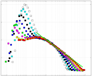
The present analysis is based on the nanoscale thermal anemometry probe (NSTAP) data measured in the Princeton Superpipe (Hultmark et al. Reference Hultmark, Vallikivi, Bailey and Smits2012). Figure 1 shows scaling of the streamwise variance with length scale,  $y_m^+ = 3.5 \sqrt {Re_{\tau }}$, and velocity scale,
  $u_m = \sqrt {\overline {u^2}} (y=y_m)$. As can be seen, there is an excellent collapse of the profiles in the region around
  $y / y_m = 1$ for two decades in
  $Re_\tau$,
  $1985 \le Re_{\tau } \le 98\,190$: this is the motivation for using
  $u_m$ as the intermediate velocity scale. At the highest Reynolds numbers, the scaled region extends from
  $0.15 \leq y/y_m \leq 15$ and, as expected, the profiles peel off from this trend on both sides of
  $y/y_m = 1$ as
  $Re_{\tau }$ decreases. The choice of constant used in the definition of
  $y_m^+$ is guided by the coefficients for
  $\sqrt {Re_{\tau }}$ used in previous definitions of the mesolayer location, e.g.
  $2\sqrt {Re_{\tau }}$ (Sreenivasan & Sahay Reference Sreenivasan and Sahay1997), or in determining the lower bound of the inertial sublayer,
  $3\sqrt {Re_{\tau }}$ (Marusic et al. Reference Marusic, Monty, Hultmark and Smits2013). Here, a slightly higher value, 3.5, is chosen to provide a better
  $Re_{\tau }$ scaling of the variance profiles for the pipe as well as boundary layer data (not shown); see Diwan & Morrison (Reference Diwan and Morrison2019). Note that the qualitative (and, to certain extent, quantitative) nature of the results is unaffected by the precise choice of this constant. Taking
  $U_m$ as the mean velocity at
  $y = y_m$, figure 2 shows, in ‘defect’ form, the corresponding mean velocity profiles scaled on
  $u_m$. Excellent scaling is apparent around
  $y/y_m = 1$ for mean velocity also. This scaling for the mean velocity and variance suggests the existence of a distinct, asymptotic intermediate layer lying between the classical inner and outer layers. This implies that there exists two overlap regions: one between the inner and intermediate layers (‘Overlap Layer I’) and the other between the intermediate and outer layers (‘Overlap Layer II’); see also Afzal (Reference Afzal1982). We choose the velocity scales in the inner and outer layers as
  $u_i$ and
  $u_o$, respectively, which in general need not be the same as
  $u_m$. This is in contrast to the earlier formulations (Afzal Reference Afzal1982; Sreenivasan & Sahay Reference Sreenivasan and Sahay1997; Klewicki Reference Klewicki2013), which used the same velocity scale,
  $u_{\tau }$, for all the layers considered. The use of
  $u_m$ instead of
  $u_{\tau }$ in our formulation enables the demonstration of Reynolds-number similarity in the intermediate layer of the pipe (figures 1, 2). Note that the five-layer description based on spectral characteristics of the streamwise velocity proposed by Vallikivi, Ganapathisubramani & Smits (Reference Vallikivi, Ganapathisubramani and Smits2015) is different in spirit to the present formulation which, including the two overlap layers, also proposes a total of five layers. Next, we carry out a matching analysis using the method used by Zagarola & Smits (Reference Zagarola and Smits1998). For Overlap Layer I, the inner and intermediate scaling laws are written as
 \begin{equation} U^+= f(y^+), \quad \frac {U-U_m} {u_m} = g(\zeta), \end{equation}
where  $\zeta = y/y_m$. Asymptotic matching of the velocity gradient for the inner and intermediate layers gives
 \begin{equation} y^+ f^{\prime} (y^+) = \varLambda_{I} \zeta g^{\prime}(\zeta), \end{equation}
where  $\varLambda _{I} = u_m / u_{\tau }$ and
  $(^\prime )$ indicates the derivative with respect to the corresponding independent variable. When
  $\varLambda _I$ is Reynolds-number dependent, (2.2) does not imply log-law scaling. For this case, Reynolds-number similarity can be achieved by simultaneously matching both velocity and velocity gradient in the overlap region. This results in a power law for the mean velocity:
 \begin{equation} \left.\begin{gathered} f(y^+) = U^+= C (y^+) ^ \gamma, \\ \frac{U_m}{u_m} + g(\zeta) = \frac{U}{u_m} = C_m \left(\frac{y}{y_m} \right) ^ \gamma, \end{gathered}\right\} \end{equation}
where  $\gamma$,
  $C$ and
  $C_m$ are constants. Alternatively, when
  $\varLambda _I$ = constant, a log law is obtained in the overlap region.

Figure 1. Streamwise variance profiles in a smooth pipe scaled on the intermediate variables  $y_m$ and
  $u_m$; data from Hultmark et al. (Reference Hultmark, Vallikivi, Bailey and Smits2012). The solid line is the log-law fit.

Figure 2. Streamwise mean velocity deficit scaled on the intermediate variables. The magenta line indicates a power-law fit and the green line indicates the log-law fit. The inset shows the variation without the power and log law lines.
Figure 3(a) shows the variation of  $\varLambda _I$ with Reynolds number, where it continues to increase even at the highest
  $Re_{\tau }$. This implies that Overlap Layer I is governed by a power law up to
  $Re_\tau \approx 10^5$. The ratio
  $U_m/u_m$ shows a much weaker variation with
  $Re_{\tau }$ than
  $\varLambda _I$, without a monotonic trend (figure 3b): there is only a
  $6\,\%$ variation in
  $U_m/u_m$ for two decades of change in
  $Re_{\tau }$; this justifies the power law in (2.3). Fitting a power-law curve to
  $U/u_m$ for
  $0.06 \leq y/y_m \leq 0.8$,
  $Re_{\tau } = 98\,190$ gives the power-law constants as
  $\gamma = 0.14$ and
  $C_m = 8.51$. Note that
  $\gamma$ is independent of
  $Re_{\tau }$, whereas
  $C_m$ shows a weak
  $Re_{\tau }$-dependence reflecting the weak trend of
  $U_m/u_m$ with
  $Re_{\tau }$ (figure 3b). Using these parameters, the variation of
  $(U - U_m) / u_m$ is plotted in figure 2 as a magenta line which fits the data quite well in Overlap Layer I. To determine
  $C$, we separately fit a power law to the inner-scaled data (not shown here) for
  $Re_{\tau } = 98\,190$ in the corresponding range,
  $65 \leq y^+ \leq 880$ (Hultmark et al. Reference Hultmark, Vallikivi, Bailey and Smits2012). This yields the same value of
  $\gamma =0.14$, with
  $C = 8.47$. These are close to the values
  $\gamma = 0.142$ and
  $C = 8.48$ reported by McKeon et al. (Reference McKeon, Li, Jiang, Morrison and Smits2004). Overlap Layer II is bounded by the intermediate layer and the outer layer. The scaling law for the mean velocity deficit in the outer layer can be written as
 \begin{equation} \frac {U_{CL}-U} {u_o} = h\left(\frac{y}{R}\right), \end{equation}
where  $U_{CL}$ is the pipe centre-line velocity. It can be seen that the character of the mean velocity variation in Overlap Layer II is determined by the velocity-scale ratio,
  $\varLambda _{II} = u_o / u_m$ (corresponding to
  $\varLambda _{I}$ in 2.2). Note that although (2.4) is written in a Reynolds-number-invariant form, the appropriate velocity scale,
  $u_o$, that would result in Reynolds-number similarity in the outer region is still unknown (Morrison et al. Reference Morrison, McKeon, Jiang and Smits2004). The two alternatives for
  $u_o$ that have been used so far, for the pipe, are
  $u_{\tau }$ and
  $U_{CL}-U_b$ (Zagarola & Smits Reference Zagarola and Smits1998), where
  $U_b$ is the bulk velocity. Choosing
  $u_o = u_{\tau }$,
  $\varLambda _{II} = 1 / \varLambda _{I}$, implying (figure 3a) that Overlap Layer II is also governed by a power law for the entire
  $Re_{\tau }$ range. This would be a surprising result as there has been overwhelming support in favour of the log law. If, on the other hand, we choose
  $u_o = (U_{CL} - U_b)$, we get
  $\varLambda _{II} = (U_{CL} - U_b) / u_m$, see figure 3(c), which shows that
  $\varLambda _{II}$ is a strong function of
  $Re_{\tau }$, but where, for
  $Re_{\tau } \gtrsim 10^4$, it shows a much weaker dependence on
  $Re_{\tau }$. If we assume
  $\varLambda _{II}$ to be approximately constant for
  $Re_{\tau } \gtrsim 10^4$, we recover the log law for the mean velocity in Overlap Layer II, which, in terms of
  $u_m$ and
  $y_m$, can be written as
 \begin{equation} \frac{U - U_m}{u_m} = \frac{1}{\kappa_m} \ln \left(\frac{y}{y_m}\right) + A_m. \end{equation}
To obtain  $\kappa _m$ and
  $A_m$, we fit a least-square straight line through the mean velocity data (green solid line in figure 2) for the two highest Reynolds numbers,
  $Re_{\tau } = 68\,370$ and
  $Re_{\tau } = 98\,190$, and for
  $1.2 \leq (y/y_m) \leq 13$, equivalent to
  $4.2\sqrt {Re_{\tau }} \leq y^+ \leq 0.145 Re_{\tau }$ for
  $Re_{\tau } = 98\,190$, which is broadly consistent with the range used in Marusic et al. (Reference Marusic, Monty, Hultmark and Smits2013). The fit gives the following values for the constants:
 \begin{equation} \kappa_m = 1.034, \quad A_m = 0.0084. \end{equation}
These represent the Reynolds-number-invariant log-law constants in terms of the intermediate variables for  $Re_{\tau } \gtrsim 10^4$. Note that, provided the Reynolds-number similarity in the intermediate layer is ensured, the value of
  $\kappa _m$ is independent of small changes in the numerical value of the coefficient in the definition of
  $y_m$. The value of
  $A_m$, however, is directly dependent on this choice (2.5). Moreover, the range
  $1.2 \leq (y/y_m) \leq 13$ is valid only for the two highest
  $Re_{\tau }$. As
  $Re_{\tau }$ decreases, the range of
  $y/y_m$ over which a log variation is observed continues to decrease, although
  $\kappa_m$ and
  $A_m$ remain the same, as clearly seen in figure 2. To further support this observation, we plot the variation of an ‘indicator function’ (McKeon et al. Reference McKeon, Li, Jiang, Morrison and Smits2004) with
  $Re_{\tau }$, which is presented as supplementary material to this paper available at https://doi.org/10.1017/jfm.2021.71.

Figure 3. Variation with  $Re_{\tau }$ of (a)
  $\varLambda _I = u_m / u_{\tau }$, (b)
  $U_m/u_m$, (c)
  $\varLambda _{II} = (U_{CL} - U_b) / u_m$, (d)
  $\kappa$ obtained from (3.1a,b); the values of
  $\kappa$ for
  $Re_{\tau } \lesssim 10^4$ do not correspond to the log law and are shown by crosses.
In figure 1, the Reynolds-number similarity of the streamwise variance for  $y \approx y_m$ implies that, for
  $y > y_m$, there should exist a Reynolds-number-invariant log law for the variance as well (scaled on the intermediate variables), which is
 \begin{equation} \frac {\overline{u^2}} {u_{m}^2} = B^m_1 - A^m_1 \ln \left( \frac{y}{y_m} \right). \end{equation}
To determine  $A^m_1$ and
  $B^m_1$, we fit a least-square straight line through the points in figure 1 (shown as a solid line) in the region
  $1.2 \leq y/y_m \leq 13$ for the two highest Reynolds numbers; this range is the same as that chosen for fitting the log law for the mean velocity in Overlap Layer II (figure 2). Again the extent of the log region for the variance decreases with decrease in
  $Re_{\tau }$; see the supplementary material for the indicator-function plots. (The behaviour of
  $\overline {u^2}$ in Overlap Layer I is beyond the scope of the present work.) This line fit gives the
  $Re$-invariant log-law constants for the streamwise variance as
 \begin{equation} A^m_1 = 0.178, \quad B^m_1 = 1.005. \end{equation}
We do not attempt to estimate the uncertainty bounds for  $A^m_1$ and
  $B^m_1$, nor for
  $\kappa _m$ and
  $A_m$, (2.6a,b) here, as their precise numerical values are not relevant for our key conclusions.
3. Consequences for the von Kármán and Townsend–Perry ‘constants’
The classical log-law constants for the mean velocity and variance can be readily expressed in terms of the constants obtained from the intermediate-scaled log laws. For the mean velocity, this relation can be written as (1.1), (2.5)
 \begin{equation} \kappa = \frac{\kappa_m} {(u_m / u_{\tau})},\quad A = \frac{u_m}{u_{\tau}} \left\{\left[\frac{U_m}{u_m} + A_m\right] - \frac{1}{\kappa_m} \ln (y_m^+) \right\}. \end{equation}
The value of  $\kappa$ obtained from (3.1a,b) is plotted in figure 3(d); see also table 1. For
  $Re_{\tau } > 2 \times 10^4$,
  $\kappa$ falls within the range
  $0.4 \pm 0.02$ (Bailey et al. Reference Bailey, Vallikivi, Hultmark and Smits2014), shown as dashed lines in the figure; the trend exhibited by
  $\kappa$ within the band reflects the variation of
  $u_m/u_{\tau }$ with
  $Re_{\tau }$ (figure 3a; 3.1a,b). For
  $Re_{\tau } < 10^4$, the values of
  $\kappa$ are found to be much higher than those which could be reasonably associated with a log law. These are denoted as crosses in figure 3(d), including
  $\kappa =0.43$ at
  $Re_{\tau } = 10\,480$ which falls beyond the band of
  $0.4 \pm 0.02$. This suggests that the mean velocity profile in Overlap Layer II is better described by a power law at lower
  $Re_{\tau }$, as implied by the strong Reynolds-number dependence of
  $\varLambda _{II}$ for
  $Re_{\tau } \lesssim 10^4$ (figure 3c). Note that Overlap Layer I is governed by power law for all
  $Re_{\tau }$ considered here. For
  $Re_{\tau } < 10^4$, the two overlap layers may not be entirely distinct and therefore the two power-law profiles may appear indistinguishable (figure 2). These results are consistent with those in Zagarola & Smits (Reference Zagarola and Smits1998) and McKeon et al. (Reference McKeon, Li, Jiang, Morrison and Smits2004).
Table 1. The log-law constants for the mean velocity ( $\kappa$ and
  $A$) and variance (
 $A_1$ and
  $B_1$) obtained from (3.1a,b) and (3.2a,b) using the log fits in (2.5) and (2.7). For
  $Re_{\tau } \leq 10,480$,
  $\kappa$ and
  $A$ are shown as ‘
 $\times$’ as log law is not expected in Overlap Layer II (figure 3d).

The presence of a power law in Overlap Layer I and of the log law in Overlap Layer II, for  $Re_{\tau } > 2 \times 10^4$, supports the observation by Zagarola & Smits (Reference Zagarola and Smits1998) (see also Hultmark et al. Reference Hultmark, Vallikivi, Bailey and Smits2012) that, at high
  $Re_{\tau }$, the mean velocity initially follows a power law, with a log law at larger
  $y$. Note that in their analysis, the power and log laws share the same overlap region, whereas in the present three-layer formulation they occupy two different overlap regions. This provides an explanation for the coexistence of the power and log-law profiles in the pipe flow at a given (and sufficiently large)
  $Re_{\tau }$. Furthermore, since the length scale for the intermediate layer is
  $\propto \sqrt {Re_{\tau }}$, the lower limit for the log law for the mean velocity should be Reynolds-number dependent, rather than constant in wall variables: see the discussion in Marusic et al. (Reference Marusic, Monty, Hultmark and Smits2013) and Bailey et al. (Reference Bailey, Vallikivi, Hultmark and Smits2014).
For the variance, the classical constants,  $A_1$ and
  $B_1$ (1.2), can be expressed in terms of
  $A^m_1$ and
  $B^m_1$ (2.7) as
 \begin{equation} A_1 = A_1^m \left( \frac {u_m^2} {u_{\tau}^2} \right),\quad B_1 = \left[A_1^m \ln \left(\frac {y_m} {R} \right) + B_1^m \right] \left( \frac {u_m^2} {u_{\tau}^2} \right). \end{equation}
Values of  $A_1$ and
  $B_1$ calculated from (3.2a,b) (with
  $A^m_1 = 0.178$ and
  $B^m_1 = 1.005$) are included in table 1; a clear trend in
  $A_1$ and
  $B_1$ with respect to
  $Re_{\tau }$ is evident. Figure 4 shows the log-law fits to the variance, in wall variables, obtained by using
  $A_1$ and
  $B_1$ from table 1. As can be seen, the log fits inferred from (3.2a,b) show a good match with the measured profiles in the intermediate region, over the entire
  $Re_{\tau }$ range. This leads us to conclude that the Townsend–Perry ‘constant’,
  $A_1$, actually shows a systematic dependence on
  $Re_{\tau }$ even for
  $Re_{\tau } > 10^4$. This is due to the fact that
  $A^m_1$ and
  $B^m_1$ are
  $Re_{\tau }$-invariant and that
  $u_m/u_{\tau }$ (figure 3a) and
  $y_m/R\ (=3.5/\sqrt {Re_{\tau }})$ show a continuous dependence on
  $Re_{\tau }$. Furthermore, the values of
  $A_1$ in table 1 are entirely consistent, at corresponding Reynolds numbers, with those in Perry et al. (Reference Perry, Henbest and Chong1986) (
 $A_1 = 0.9$ for
  $Re_{\tau } \leq 3900$) and Hultmark et al. (Reference Hultmark, Vallikivi, Bailey and Smits2012) (
 $A_1 = 1.25$ for
  $Re_{\tau } = 98\,190$; Marusic et al. (Reference Marusic, Monty, Hultmark and Smits2013) reported
  $A_1 = 1.23\pm 0.05$ for the same
  $Re_{\tau }$). Hence, the use of the three-layer formulation and intermediate scaling enable us to explain the
  $Re_{\tau }$-dependence of
  $A_1$, providing both an explanation for the low values of
  $A_1$ obtained by Perry et al. (Reference Perry, Henbest and Chong1986), as well as reproducing
  $A_1 \approx 1.25$ for the high-
 $Re$ data. Another advantage of this framework is that the extent of the log region for different
  $Re_{\tau }$ in the classical scaling (figure 4) is automatically determined once the extent of the intermediate-scaled log law (2.7), (3.2a,b) is known. This removes the subjectivity of fitting a log law to the variance data, which has a direct bearing on the determination of
  $A_1$. The same considerations also apply to the determination of
  $\kappa$ for the mean velocity (table 1).

Figure 4. Streamwise variance profiles for the pipe; solid lines are the classical log-law fits using  $A_1$ and
  $B_1$ from table 1.
Note that the values of  $A_1$ and
  $B_1$ are listed for all
  $Re_{\tau }$ in table 1, whereas those for
  $\kappa$ and
  $A$ are listed only for
  $Re_{\tau } > 2 \times 10^4$, below which we expect a power law. However, there is no general principle to rule out the presence of log law in
  $\overline {u^2}$ at
  $Re_{\tau } \lesssim 10^4$ apart from low-Reynolds-number effects. In addition, indicator functions for
  $\overline {u^2}$ suggest the presence of a log law for the entire range of
  $Re_{\tau }$. Of course, the numerical values of
  $\kappa$ and
  $A_1$ (and also
  $A$ and
  $B_1$) in table 1 and their precise variation with
  $Re_{\tau }$ are contingent on the accuracy of the data used for fitting the intermediate-scaled log laws. Vallikivi (Reference Vallikivi2014) estimates uncertainties in the NSTAP measurement,
  $U$, to be
  ${\pm }2.2\,\%$, the corresponding uncertainty in
  $\overline {u^2}$ being
  ${\pm }3.0\,\%$. Using the mean momentum equation, the associated error in
  $\overline {uv}$ (where
  $v$ is the radial velocity component) is expected to be approximately
  ${\pm }5\,\%$. These estimates can be usefully compared to the Pitot probe data from McKeon (Reference McKeon2004) which estimates the corresponding uncertainties in
  $U$ to be
  ${\pm }0.3\,\%$. However, here obviously one does not have the higher-order statistics provided by the NSTAP probe. Nonetheless, as table 1 shows, the present analysis using the NSTAP data provides estimates of
  $\kappa$ and
  $A$ that are consistent with the earlier Pitot probe data from the Superpipe. We therefore expect the three-layer structure to be apparent for both data sets.
4. Discussion
The choice of  $u_m$ as a velocity scale is not obvious, the
  $u$-component comprising both the ‘active’ shear-stress-bearing motion of the inner layer (the ‘large-scale motions’, LSM) and that induced by the ‘very-large-scale motions’ (VLSM) residing primarily in the outer layer (Marusic et al. Reference Marusic, McKeon, Monkewitz, Nagib, Smits and Sreenivasan2010). The intermediate layer can be conceived as a region in which both the LSM and VLSM are of comparable magnitude, as suggested by the spectral analysis of Vallikivi et al. (Reference Vallikivi, Ganapathisubramani and Smits2015). Thus, the intermediate layer in pipe flow is a central site for inner-outer interaction (Morrison Reference Morrison2007; Marusic et al. Reference Marusic, McKeon, Monkewitz, Nagib, Smits and Sreenivasan2010). Further, the peak in shear stress,
  $-\overline {uv}$ (figure 5), is close to the outer peak in
  $\overline {u^2}$ (figure 1), which is the lower limit to the log law; see figure 6. The log region makes a major contribution to the bulk production of turbulence kinetic energy at high
  $Re_{\tau }$, and is likely to enhance levels of
  $\overline {u^2}$ in the intermediate region (Hultmark et al. Reference Hultmark, Vallikivi, Bailey and Smits2012). The causal connection between
  $-\overline {uv}$ and
  $\overline {u^2}$ in a fully developed internal flow is clearly provided through the production of
  $\overline {u^2},~\overline {uv} (\textrm {d} U/{\textrm {d}y})$. More specifically, we note that, in the local-equilibrium region, the non-dimensional dissipation rate,
  ${\epsilon }/{u_\tau ^3/R} \propto \sqrt {Re_\tau }$ (Morrison & Fernandez Vicente Reference Morrison and Fernandez Vicente2019), implying that
  $u_m$, as a scale for
  $\overline {u^2}$, is also relevant to
  $-\overline {uv}$.

Figure 5. The deficit in  $-\overline {uv}$ scaled on the intermediate variables, i.e.
  $3.5/\sqrt {Re_{\tau }} (=y_m/R)$ and
  $u_m/u_{\tau }$, as a function of
  $y/y_m$. See figure 4 for the legend.

Figure 6. Variation of three length scales,  $y^+=5, y^+_m, R^+$, and locations of peaks in
  $-\overline {uv}$,
  $-\overline {uv} (\textrm {d} U/{\textrm {d}y})$ and
  $\overline {u^2}$. There is some uncertainty in determining the location of the peak in
  $-\overline {uv}$ for the two largest
  $Re_{\tau }$ (figure 5 inset), which is typically the same as the size of the symbols.
We consider the mean momentum balance for the turbulent pipe flow as follows:
 \begin{equation} \nu \frac{\textrm{d}^2U}{{\textrm{d}y}^2} + \frac{\textrm{d}}{\textrm{d}y} (-\overline{uv}) ={-} \frac{u^2_{\tau}}{R} \left({\equiv} \frac{1}{\rho} \frac{\textrm{d} p}{\textrm{d}x}\right). \end{equation}
Its scaling behaviour in the classical inner and outer layers is well-known (Afzal Reference Afzal1982; Klewicki Reference Klewicki2013). To investigate the leading-order force balance in the intermediate layer, we introduce the intermediate-scaled mean velocity deficit (2.1a,b). For scaling the Reynolds stress gradient, we use the observation that the deficit in the maximum Reynolds shear stress,  $(-\overline {uv}_{max} - u_{\tau }^2)/u_{\tau }^2$, scales on
  $1/\sqrt {Re_{\tau }}$ (Afzal Reference Afzal1982; Sreenivasan & Sahay Reference Sreenivasan and Sahay1997). With intermediate scaling, (4.1) can be rearranged in deficit form as:
 \begin{equation} \frac{1}{(3.5)^2} \frac{\textrm{d}^2}{\textrm{d}\zeta^2} \left( \frac{U - U_m}{u_m} \right) + \frac{\textrm{d}}{\textrm{d}\zeta} \left[\left( \frac{-\overline{u v} - u_{\tau}^2} {u_{\tau}^2} \right) \left( \frac{\sqrt{Re_{\tau}}}{3.5} \right) \frac{u_{\tau}}{u_m} \right]={-}\frac{u_{\tau}}{u_m}. \end{equation}
The quantity in square brackets on the left-hand side in (4.2), the Reynolds-stress deficit, is plotted in figure 5 as a function of  $\zeta =y/y_m$; the inset shows an expanded view of the peak in
  $-\overline {uv}$. The
  $-\overline {uv}$ data are obtained from (4.1) using the mean velocity data (figure 2): figure 5 shows that intermediate scales work well in the intermediate layer. This collapse is consistent with that seen earlier for
  $\overline {u^2}$ (figure 1) and
  $(U-U_m)$ (figure 2). The term
  $u_{\tau }/u_m$ on the right-hand side of (4.2) implies that the leading-order force balance, under the intermediate scaling, is approximate so long as
  $u_{\tau }/u_m$ is a function of
  $Re_{\tau }$, and can be expected to become exact as
  $Re_\tau \rightarrow \infty$. However, it is clear that the intermediate scaling presents a ‘distinguished limit’ distinct from the inner and outer limits (Afzal Reference Afzal1982). If the ratio
  $\varLambda _I = u_m/u_{\tau }$ (and
  $\varLambda _{II}= u_o/u_m$) reaches a constant value as
  $Re_{\tau } \to \infty$, the present analysis becomes identical with that in Afzal (Reference Afzal1982), with all the three layers governed by
  $u_{\tau }$. Clearly this limit has not yet been reached for the present data, as
  $u_m$ continues to be a relevant velocity scale in the intermediate layer even for
  $Re_{\tau } = O(10^5)$; see figures 1–3. Note that the balance of forces in (4.2) is consistent with that obtained in layer III in the analysis of Klewicki (Reference Klewicki2013).
As a distinguished limit, the intermediate layer has distinct underlying physics, unique to its position in the wall layer. This becomes evident by looking at figure 6, which plots positions of the three layers in relation to locations of peaks in  $-\overline {uv}$,
  $-\overline {uv} (\textrm {d} U/{\textrm {d}y})$ and
  $\overline {u^2}$. As can be seen, the peak in production (
 $y^+=12$) and the inner peak in
  $\overline {u^2}$ (
 $y^+ \approx 15$; Hultmark et al. Reference Hultmark, Vallikivi, Bailey and Smits2012) characterise the inner layer. Correspondingly, the peak in Reynolds shear stress and the outer peak in
  $\overline {u^2}$ (given by
  $y^+ = 0.23(Re_{\tau })^{0.67}$; Hultmark et al. Reference Hultmark, Vallikivi, Bailey and Smits2012) are seen to characterise the intermediate layer; see figure 6. The intermediate layer is amenable to another interesting physical interpretation: in the context of their mesolayer theory, Sreenivasan & Sahay (Reference Sreenivasan and Sahay1997) proposed that the peak in
  $-\overline {uv}$ could play a role similar to that of the ‘critical layer’ in unstable wall flows. They pointed out that the mean velocity at the
  $(-\overline {uv})_{max}$ location is approximately a constant fraction (
 $=0.65$) of the centre-line velocity in the pipe, similar to that for a critical layer. In the present work,
  $U_m / U_{CL}$ falls in the range 0.68–0.64 for
  $Re_{\tau } = 1985\text {--}98\,190$ and for
  $Re_{\tau } > 20\,000$,
  $U_m / U_{CL} \approx 0.65$.
5. Conclusion
We have shown that, using intermediate variables ( $y_m, u_m$), the streamwise mean velocity deficit and variance exhibit Reynolds-number similarity in the intermediate region of the pipe flow. This suggests a three-layer asymptotic formulation for pipe flow, with two overlap layers (Afzal Reference Afzal1982), wherein the intermediate layer is governed by a velocity scale (
 $u_m$) different from the friction velocity. A generalised matching analysis shows that Overlap Layer I (nearer to the wall) is governed by a power law for the mean velocity until
  $Re_{\tau } = O(10^5)$ and that the log law emerges in Overlap Layer II for
  $Re_{\tau } \gtrsim 10^4$. This provides a theoretical explanation for the presence of a power law close to the wall and a log law further away, as observed in the Superpipe measurements of Zagarola & Smits (Reference Zagarola and Smits1998) and Hultmark et al. (Reference Hultmark, Vallikivi, Bailey and Smits2012).
In terms of the intermediate scaling, Overlap Layer II (which represents the inertial sublayer) exhibits a Reynolds-number-invariant log law for the mean velocity deficit (at high  $Re_{\tau }$) as well as the variance. The von Kármán (
 $\kappa$) and Townsend–Perry (
 $A_1$) ‘constants’ have been derived from the intermediate-scaled log-law constants. We find that
  $\kappa$ shows a weak trend within the range
  $0.4 \pm 0.02$ for
  $Re_{\tau } > 2 \times 10^4$ consistent with the literature, whereas
  $A_1$ exhibits a systematic Reynolds-number dependence up to the highest available
  $Re_{\tau }$. The present formulation shows that the scale separation between two adjacent layers is proportional to
  $\sqrt {Re_{\tau }}$ (rather than
  $Re_{\tau }$) and this is likely to explain the slow approach to asymptotic conditions (in terms of classical variables) evident in the pipe flow data.
Supplementary material
Supplementary material is available at https://doi.org/10.1017/jfm.2021.71.
Acknowledgements
We are grateful to Professor A. Smits for use of the NSTAP data and for useful discussions. We thank Professor J. Klewicki for his comments on the mean momentum analysis, and the referees for useful suggestions that have helped to improve the paper.
Funding
We acknowledge financial support from EPSRC under Grant No. EP/I037938/1.
Declaration of interests
The authors report no conflict of interest.


