


1 Introduction
This paper is motivated by the potential of compliant panels to interact favourably with the dynamics of boundary-layer flows and thereby yield a reduction to skin-friction drag. The investigation focuses upon instability mechanisms that can lead to laminar-to-turbulent transition in low disturbance environments for zero pressure gradient boundary-layer flow although the new modelling approach developed is readily extended to the study of other wall-bounded mean shear flows with a deformable boundary.
There exists a rich literature on the topic of ‘compliant walls for transition delay’ spanning the nearly sixty years since the pioneering experimental work of Kramer (Reference Kramer1957, Reference Kramer1960); this has been summarised periodically through review articles (Benjamin Reference Benjamin1963; Bushnell Reference Bushnell1977; Carpenter Reference Carpenter1991; Gad-el-Hak Reference Gad-el-Hak1998; Carpenter, Davies & Lucey Reference Carpenter, Davies and Lucey2001) that chronicle the development of the field of study. The principal engineering outcome to date is that optimally designed compliant coatings could extend the length of the linear transition regime by a factor of 5.7 (Dixon, Lucey & Carpenter Reference Dixon, Lucey and Carpenter1994) and the prediction, argued in Carpenter et al. (Reference Carpenter, Davies and Lucey2001), that a series of compliant panels, each with properties tailored to local mean flow, could theoretically postpone transition indefinitely. In contrast, a focus over the last decade or so on establishing a theoretical framework for compliant wall interactions with turbulent boundary layers (Rempfer et al. Reference Rempfer, Blossey, Parsons and Lumley2001; Xu, Rempfer & Lumley Reference Xu, Rempfer and Lumley2003; Fukagata et al. Reference Fukagata, Kern, Chatelain, Koumoutsakos and Kasagi2008; Kim & Choi Reference Kim and Choi2014; Luhar, Sharma & McKeon Reference Luhar, Sharma and McKeon2015, Reference Luhar, Sharma and McKeon2016) to understand, inter alia, the experimentally measured drag reductions in Choi et al. (Reference Choi, Yang, Clayton, Glover, Atlar, Semenov and Kulik1997) at present suggests that only limited benefits are conferred by wall compliance. Competing passive technologies such as the use of riblets currently offer a more practicable strategy for drag reduction in turbulent boundary-layer flow. Nevertheless, the technological prospect of turbulent skin-friction drag reduction using wall compliance remains an open question. However, the present study returns to the theme of transition postponement and serves to yield a complete understanding of the interaction of laminar boundary-layer flow with compliant panels, i.e. compliant coatings of finite streamwise extent. A schematic of the system studied is presented in figure 1.

Figure 1. Schematic of the system studied with nomenclature.
Hitherto, theoretical studies of laminar boundary-layer flow over a compliant wall have been undertaken mainly using two-dimensional (2-D) (Carpenter & Garrad Reference Carpenter and Garrad1985, Reference Carpenter and Garrad1986; Sen & Arora Reference Sen and Arora1988) or three-dimensional (3-D) (Joslin, Morris & Carpenter Reference Joslin, Morris and Carpenter1991; Joslin & Morris Reference Joslin and Morris1992; Yeo Reference Yeo1992; Zengl & Rist Reference Zengl, Rist, Tropea and Bleckmann2012) linear temporal or spatial local stability analyses based on the assumption of a compliant wall of infinite extent. Numerical simulations of compliant panels interacting with laminar shear flow have been performed for linear (Davies & Carpenter Reference Davies and Carpenter1997b ) and nonlinear (Wiplier & Ehrenstein Reference Wiplier and Ehrenstein2000, Reference Wiplier and Ehrenstein2001; Pavlov Reference Pavlov2006) system perturbations but these have been limited by the choice of type and frequency of the initial disturbance and therefore their results pertain to a limited domain within the overall stability space. Emphasis has been placed on the effect of surface-based or volume-based isotropic and anisotropic compliant walls (Yeo & Dowling Reference Yeo and Dowling1987; Yeo Reference Yeo1988, Reference Yeo1990; Carpenter & Morris Reference Carpenter and Morris1990; Pavlov Reference Pavlov2006; Zengl & Rist Reference Zengl, Rist, Tropea and Bleckmann2012) on both 2-D and 3-D instabilities in order to identify rationally coating parameters (Carpenter Reference Carpenter1993; Dixon et al. Reference Dixon, Lucey and Carpenter1994) that are suitable for postponing the onset of spatially growing instabilities to higher Reynolds numbers (hence distance downstream of the leading edge in applications) or reducing their amplification. Using the aforementioned techniques, three types of instability have been identified and categorised as: (i) flow-based instabilities, (ii) flow-induced wall-based instabilities and (iii) instabilities arising from linear modal interactions. These types of instability are each expanded upon in the following three paragraphs.
Amplifying Tollmien–Schlichting Waves (TSWs) (Schlichting Reference Schlichting1979) comprise the main flow-based instability; these are also responsible for natural transition to turbulence in flat-plate boundary-layer flow over rigid walls in low disturbance environments. However, in a convective 2-D boundary-layer flow, an additional flow-based transient mechanism exists, namely the Orr instability (Orr Reference Orr1907; Butler & Farrell Reference Butler and Farrell1992; Åkervik et al. Reference Åkervik, Ehrenstein, Gallaire and Henningson2007), which extracts energy from the mean shear by transporting momentum downstream through the action of the perturbation Reynolds stress. Disturbances, which are tilted against the shear first rise to an upright position while drawing energy from the mean flow after which energy is returned to the mean flow further downstream. This energy transfer mechanism can potentially precipitate transition to turbulence, bypassing the TSW route in natural transition.
The flow-induced wall-based instabilities principally comprise travelling wave flutter (TWF) (Carpenter & Garrad Reference Carpenter and Garrad1986; Yeo Reference Yeo1988) and static divergence (SD). TWF is the destabilisation of free surface wave modes of the compliant wall through the fluid loading and takes the form of a wave propagating downstream with a phase speed close to that of the free-stream flow. In contrast, SD (Lucey & Carpenter Reference Lucey and Carpenter1992; Pitman & Lucey Reference Pitman and Lucey2009) occurs when the hydrodynamic forces generated by a wall deformation exceed the associated restorative forces in the compliant wall and manifests itself as a slow downstream-travelling wave. Like TSWs, TWF is a convective instability with a wave amplifying only as it propagates away from the initiating source of disturbance, while SD is considered an absolute instability because the wave grows in time at all spatial locations of the domain. Even though the mechanism underlying TWF is essentially inviscid, the Orr–Sommerfeld equation can accurately predict its onset Reynolds number and subsequent propagation. However, it largely fails to predict the absolute SD (Carpenter & Morris Reference Carpenter and Morris1990) because exactly at onset the instability is static and therefore the wave-based assumption of the Orr–Sommerfeld equation is essentially invalid. A further flow-induced surface instability, associated with the tangential (axial) wall motion, was discovered by Shankar & Kumaran (Reference Shankar and Kumaran2002) when studying the local temporal stability and asymptotic analysis of Couette flow past a flexible surface. This instability occurs through energy transfer to the wall caused by the interaction of the fluctuating (fluid) shear stress and the axial motion of the wall at the fluid–solid interface. However, less is known about the character of this new instability – whether it is convective or absolute – and its interaction with structural modes or the TSW or TWF instabilities in a fluid–structure interaction (FSI) system of finite length.
The third category of instability includes transitional instability (Sen & Arora Reference Sen and Arora1988) which is generated by the coalescence of TWF and TSWs and the instability caused by the coalescence of the evanescent waves and a TSW (Wiplier & Ehrenstein Reference Wiplier and Ehrenstein2001). These instabilities are identified in a local stability analysis as a pinching of the different instability branches in the wavenumber (
 $\unicode[STIX]{x1D6FC}$
) plane for positive imaginary part of the frequency (
$\unicode[STIX]{x1D6FC}$
) plane for positive imaginary part of the frequency (
 $\unicode[STIX]{x1D714}$
) or, equivalently, as a cusp in the frequency plane (Yeo, Khoo & Zhao Reference Yeo, Khoo and Zhao1996; Wiplier & Ehrenstein Reference Wiplier and Ehrenstein2001) at the frequency where the coalescence of the two modal branches takes place. These are both absolute instabilities and, along with SD, must be avoided in compliant wall design because their occurrence is likely to result in a significant modification to the base flow (Carpenter & Morris Reference Carpenter and Morris1990; Wiplier & Ehrenstein Reference Wiplier and Ehrenstein2001) and/or premature boundary-layer transition.
$\unicode[STIX]{x1D714}$
) or, equivalently, as a cusp in the frequency plane (Yeo, Khoo & Zhao Reference Yeo, Khoo and Zhao1996; Wiplier & Ehrenstein Reference Wiplier and Ehrenstein2001) at the frequency where the coalescence of the two modal branches takes place. These are both absolute instabilities and, along with SD, must be avoided in compliant wall design because their occurrence is likely to result in a significant modification to the base flow (Carpenter & Morris Reference Carpenter and Morris1990; Wiplier & Ehrenstein Reference Wiplier and Ehrenstein2001) and/or premature boundary-layer transition.
In the energy classification of Benjamin (Reference Benjamin1963), TSWs are found to be a Class A instability because their activation energy (energy relative to the quiescent system state) is negative and they are therefore destabilised by structural damping since it removes energy from the FSI system. These waves are equivalently termed negative energy waves (NEWs) in, for example, Crighton & Oswell (Reference Crighton and Oswell1991), this description having been adopted from the plasma physics community. TWF is a Class B instability because its activation energy is positive (hence a positive energy wave in Crighton & Oswell Reference Crighton and Oswell1991) and is therefore attenuated by the action of structural damping. Finally, Class C comprises waves that are destabilised independently of whether there is irreversible energy transfer from/to the FSI system. Kelvin–Helmholtz (called modal coalescence flutter in the hydro-elasticity of flexible panels and walls) and the transitional instabilities belong to this class of instability. The SD waves have been predicted to be Class A when modelled using an infinitely long domain (e.g. Crighton & Oswell Reference Crighton and Oswell1991; Davies & Carpenter Reference Davies and Carpenter1997a ) because structural damping is required to precipitate the instability. However, for compliant panels of finite length it has been shown (Lucey & Carpenter Reference Lucey and Carpenter1992; Pitman & Lucey Reference Pitman and Lucey2009) that structural damping reverts to its conventional role and reduces the amplification of SD waves at post-critical flow speeds. In addition, its mechanism is principally due to conservative energy exchanges thereby suggesting that it is more likely to be a Class C instability.
Although local stability analyses have revealed the main physics behind the rich range of phenomena supported by the FSI system, there remain drawbacks arising from the local nature of the analysis. Specifically, it is difficult to model the boundary conditions of a compliant wall of finite extent because the analysis assumes homogeneity in the streamwise direction. The non-trivial effect on the system’s stability due to panel edges which can reflect incident waves has been emphasised by several investigations both in the potential (Lucey & Carpenter Reference Lucey and Carpenter1992; Peake Reference Peake2004; Pitman & Lucey Reference Pitman and Lucey2009) and viscous (Davies & Carpenter Reference Davies and Carpenter1997b
; Wiplier & Ehrenstein Reference Wiplier and Ehrenstein2001; Stewart, Waters & Jensen Reference Stewart, Waters and Jensen2009) flow regimes. For potential flow, Peake (Reference Peake2004) showed that a long but finite plate possesses resonant solutions and that the temporal instability is present in the absence of structural damping on the finite plate even for cases where a local analysis predicts that the flow is stable. This finding agreed with the theoretical ideas of Lucey & Carpenter (Reference Lucey and Carpenter1993) and were confirmed by numerical simulations of the system by Lucey & Carpenter (Reference Lucey and Carpenter1992). Stewart et al. (Reference Stewart, Waters and Jensen2009) demonstrated that a local analysis gives only limited insight into the properties of the global system because wave reflections at boundaries played a vital role in the growth of mode-1 oscillations in their finite-length compliant insert in the wall of a two-dimensional channel. However, it is not known whether higher-order eigenmodes of the finite structure can interact with modes of the viscous flow and whether this interaction might be identified in a local stability analysis. In addition, to study absolute instabilities that may exist in the system, the frequency must be varied in order to reveal the entire unstable wavenumber spectrum,
 $\unicode[STIX]{x1D6FC}(\unicode[STIX]{x1D714})$
, and identify the different instability branches for a specific Reynolds number and their possible pinching; this proves to be a daunting task (Yeo et al.
Reference Yeo, Khoo and Zhao1996; Wiplier & Ehrenstein Reference Wiplier and Ehrenstein2001). In parallel, it has been shown through a multiple-scale analysis (Yeo, Khoo & Chong Reference Yeo, Khoo and Chong1994) that the incorporation of non-parallel effects due to boundary-layer growth (clearly omitted in a local analysis) are destabilising for TSW and TWF instabilities for Blasius flow over a compliant wall. The modelling approach, built on global stability considerations, developed and deployed in the present paper serves to overcome the limitations of local analyses.
$\unicode[STIX]{x1D6FC}(\unicode[STIX]{x1D714})$
, and identify the different instability branches for a specific Reynolds number and their possible pinching; this proves to be a daunting task (Yeo et al.
Reference Yeo, Khoo and Zhao1996; Wiplier & Ehrenstein Reference Wiplier and Ehrenstein2001). In parallel, it has been shown through a multiple-scale analysis (Yeo, Khoo & Chong Reference Yeo, Khoo and Chong1994) that the incorporation of non-parallel effects due to boundary-layer growth (clearly omitted in a local analysis) are destabilising for TSW and TWF instabilities for Blasius flow over a compliant wall. The modelling approach, built on global stability considerations, developed and deployed in the present paper serves to overcome the limitations of local analyses.
We acknowledge that the stability of finite-length flexible plates subjected to boundary-layer flow at transonic and low subsonic flow speeds, for which plate flutter is usually the critical instability, has been well studied. Dowell (Reference Dowell1971, Reference Dowell1973) modelled the effects of a laminar boundary layer analytically while more recent work by Hashimoto, Aoyama & Nakamura (Reference Hashimoto, Aoyama and Nakamura2009) and Alder (Reference Alder2015, Reference Alder2016) incorporated the effects of turbulent boundary layers by solving the Reynolds-averaged Navier Stokes equations. The overall findings of these studies are that the boundary layer exercises a stabilising effect, as compared with potential flow predictions, on panel flutter at low supersonic Mach numbers. However, the present work represents the first fairly complete stability analysis of boundary-layer flow over a finite compliant panel at low, incompressible, flow speeds.
Advances in algorithms for the numerical solution of large non-symmetric complex generalised eigenvalue problems have resulted in the ability to extend local stability theory to two inhomogeneous directions with one homogeneous direction and this defines the term ‘bi-global’ stability. In this approach, the time asymptotic and transient behaviour for a wide variety of 2-D and 3-D flows has become attainable (Theofilis Reference Theofilis2003, Reference Theofilis2011). Based on the analysis of Cossu & Chomaz (Reference Cossu and Chomaz1997) and Chomaz (Reference Chomaz2005), Ehrenstein & Gallaire (Reference Ehrenstein and Gallaire2005) investigated the convective mechanism of the classical flat-plate boundary layer by means of an appropriate superposition of two-dimensional global modes. They found that a superposition of the damped temporal global TSW eigenmodes gave rise to a localised wave packet at the inflow boundary. The wave packet would then grow while being advected downstream, in close agreement with direct numerical simulation results. However, the transient growth in energy was only of one order in magnitude. However, Åkervik et al. (Reference Åkervik, Ehrenstein, Gallaire and Henningson2007), who identified all the modal branches, found that for a slightly non-parallel flow, many eigenmodes are needed in order to obtain a converged transient energy result and that it is the combination the Orr and TSW mechanisms which yielded the potential for large downstream amplification through transient growth.
The first study of the global stability of 2-D disturbances in plane Poiseuille flow over a compliant wall with periodic boundary conditions was conducted by Pitman & Lucey (Reference Pitman and Lucey2010), using a velocity–vorticity formulation of the Navier–Stokes equations (Davies & Carpenter Reference Davies and Carpenter2001) combined with the vortex-source sheet boundary-integral method. They found that a flexible wall with structural damping improved the global system’s temporal stability by 4 % at
 $Re=6000$
and that a compliant wall with the properties of Davies & Carpenter (Reference Davies and Carpenter1997b
) results in a significant deterioration of system stability.
$Re=6000$
and that a compliant wall with the properties of Davies & Carpenter (Reference Davies and Carpenter1997b
) results in a significant deterioration of system stability.
The present work extends the velocity–vorticity formulation combined with the generalised Helmholtz decomposition (Wu & Thompson Reference Wu and Thompson1973; Kempka et al. Reference Kempka, Strickland, Glass, Peery and Ingber1995) to the global stability of the Blasius flow over a compliant wall taking into account both vertical and axial structural displacements. This is used to investigate the asymptotic and transient behaviour of the FSI system to 2-D incident disturbances. Local spatial stability analysis is also conducted in order to validate the global stability model but also to reveal the spatial characteristics of the predicted temporal instabilities. Inhomogeneity in the streamwise direction due to the boundary conditions of the compliant panel and boundary-layer growth are incorporated in the model. All of the flow and structural eigenfrequencies and the different instability branches are obtained through the solution of a generalised eigenvalue problem. In this way, it is possible to investigate the interaction between modes and identify the conditions for temporal instability in the FSI system.
In addition, the evaluation of all eigenmodes in the present study permits the transient response of the FSI system to incident 2-D disturbances to be studied. This reveals the potential of the compliant panel either to damp out disturbances in the convectively unstable boundary-layer flow or to amplify them by transferring a significant amount of energy as they travel downstream, thereby enhancing the conditions for bypass transition. A similar investigation was conducted by Zengl & Rist (Reference Zengl, Rist, Tropea and Bleckmann2012) for isotropic and anisotropic compliant wall materials for 3-D disturbances via a local stability analysis. They found that in addition to the main mechanism for the transient growth of disturbances over a rigid wall, another oscillatory mechanism coexists in the presence of an anisotropic compliant wall but that the maximum transient growth and the time of its occurrence are hardly affected.
This paper is laid out as follows. The problem formulation is presented in § 2, where the equations for the mean Blasius flow, the 2-D flow field for the disturbances, the Helmholtz decomposition and the linear model of the compliant wall’s structural dynamics are developed for both global and local stability analyses. Thereafter, the equations that describe the linear global transient response of the FSI system to 2-D disturbances, are presented and finally the discretisation of the equations using the boundary-integral vortex-source sheet method are presented. In § 3 the choice of parameters is justified and results from global and local stability investigations are presented and discussed. Particular focus is placed upon interactions between the different types of flow- and wall-based modes for a compliant wall model that permits only vertical structural displacements. The effect of both vertical and axial structural displacements is then considered as a modification to the main stability results. The global transient response of the FSI system to 2-D incident disturbances is then presented. In § 4 we provide a summary of the main findings of the investigation and draw conclusions. Finally, we remark that the theoretical approach and the discovery of two types of global instability were presented orally at an IUTAM symposium in 2014 with a summary published (Tsigklifis & Lucey Reference Tsigklifis and Lucey2015) in a special issue that recorded the outcomes of the symposium. The present paper provides a complete description of the theoretical methods with a full investigation, including parametric dependence, of globally unstable modes, their relationships to local modes, and transient effects in boundary-layer flow over a compliant panel.
2 Problem formulation
As illustrated in figure 1, a Blasius boundary layer progresses over a rigid wall section of length
 $L_{w1}^{\prime }$
onto a compliant panel of length
$L_{w1}^{\prime }$
onto a compliant panel of length
 $L_{c}^{\prime }$
comprising a spring-backed flexible plate (that may include a dashpot-type damping) with which it interacts, and finally over a rigid wall section of length
$L_{c}^{\prime }$
comprising a spring-backed flexible plate (that may include a dashpot-type damping) with which it interacts, and finally over a rigid wall section of length
 $L_{w2}^{\prime }$
. Here and hereafter,
$L_{w2}^{\prime }$
. Here and hereafter,
 $^{\prime }$
denotes a dimensional quantity. At entry and exit (respectively distances
$^{\prime }$
denotes a dimensional quantity. At entry and exit (respectively distances
 $x_{s}^{\prime }$
and
$x_{s}^{\prime }$
and
 $x_{o}^{\prime }$
downstream from the origin of the growing boundary layer) to the domain the Reynolds number (based upon free-stream flow speed
$x_{o}^{\prime }$
downstream from the origin of the growing boundary layer) to the domain the Reynolds number (based upon free-stream flow speed
 $U_{\infty }^{\prime }$
, fluid density
$U_{\infty }^{\prime }$
, fluid density
 $\unicode[STIX]{x1D70C}_{l}^{\prime }$
and dynamic viscosity
$\unicode[STIX]{x1D70C}_{l}^{\prime }$
and dynamic viscosity
 $\unicode[STIX]{x1D707}_{l}^{\prime }$
, and boundary-layer displacement thickness
$\unicode[STIX]{x1D707}_{l}^{\prime }$
, and boundary-layer displacement thickness
 $\unicode[STIX]{x1D6FF}^{\prime }$
) are respectively
$\unicode[STIX]{x1D6FF}^{\prime }$
) are respectively
 $Re_{s}$
and
$Re_{s}$
and
 $Re_{o}$
;
$Re_{o}$
;
 $\unicode[STIX]{x1D714}_{s}^{\prime }$
and
$\unicode[STIX]{x1D714}_{s}^{\prime }$
and
 $\unicode[STIX]{x1D714}_{o}^{\prime }$
are the radian frequencies of perturbation waves that satisfy the Orr–Sommerfeld equation that serve as entry and exit conditions to the system domain.
$\unicode[STIX]{x1D714}_{o}^{\prime }$
are the radian frequencies of perturbation waves that satisfy the Orr–Sommerfeld equation that serve as entry and exit conditions to the system domain.
2.1 Mean flow field
The displacement thickness
 $\unicode[STIX]{x1D6FF}_{s}^{\prime }$
at the entrance
$\unicode[STIX]{x1D6FF}_{s}^{\prime }$
at the entrance
 $x_{s}^{\prime }$
(from the origin of the boundary layer) of the flow domain modelled provides the characteristic length scale and the free-stream flow speed,
$x_{s}^{\prime }$
(from the origin of the boundary layer) of the flow domain modelled provides the characteristic length scale and the free-stream flow speed,
 $U_{\infty }^{\prime }$
, gives the characteristic speed (hence the characteristic time is
$U_{\infty }^{\prime }$
, gives the characteristic speed (hence the characteristic time is
 $\unicode[STIX]{x1D6FF}_{s}^{\prime }/U_{\infty }^{\prime }$
). The local
$\unicode[STIX]{x1D6FF}_{s}^{\prime }/U_{\infty }^{\prime }$
). The local
 $Re_{x}$
at a position
$Re_{x}$
at a position
 $x$
of the flow field relates to the
$x$
of the flow field relates to the
 $Re_{s}$
at the entrance of the domain through
$Re_{s}$
at the entrance of the domain through
 $Re_{x}=\unicode[STIX]{x1D6FE}\sqrt{xRe_{s}}$
wherein
$Re_{x}=\unicode[STIX]{x1D6FE}\sqrt{xRe_{s}}$
wherein
 $Re_{s}=\unicode[STIX]{x1D70C}_{l}^{\prime }U_{\infty }^{\prime }\unicode[STIX]{x1D6FF}_{s}^{\prime }/\unicode[STIX]{x1D707}_{l}^{\prime }$
and
$Re_{s}=\unicode[STIX]{x1D70C}_{l}^{\prime }U_{\infty }^{\prime }\unicode[STIX]{x1D6FF}_{s}^{\prime }/\unicode[STIX]{x1D707}_{l}^{\prime }$
and
 $\unicode[STIX]{x1D6FE}=1.7208$
for the Blasius boundary layer. The horizontal and vertical velocity components of the mean flow are given by
$\unicode[STIX]{x1D6FE}=1.7208$
for the Blasius boundary layer. The horizontal and vertical velocity components of the mean flow are given by
 $$\begin{eqnarray}U_{x}=\frac{\text{d}\,f}{\text{d}H}\quad \text{and}\quad U_{z}=\frac{\unicode[STIX]{x1D6FE}}{2\sqrt{xRe_{s}}}\left(H\frac{\text{d}\,f}{\text{d}H}-f\right),\end{eqnarray}$$
where
 $H=z/(\unicode[STIX]{x1D6FE}\sqrt{x/Re_{s}})$
and
$H=z/(\unicode[STIX]{x1D6FE}\sqrt{x/Re_{s}})$
and
 $f(H)$
satisfies the Blasius equation,
$f(H)$
satisfies the Blasius equation,
 $$\begin{eqnarray}\displaystyle 2\frac{\text{d}^{3}f}{\text{d}H^{3}}+\unicode[STIX]{x1D6FE}^{2}f\frac{\text{d}^{2}f}{\text{d}H^{2}}=0, & & \displaystyle\end{eqnarray}$$
subject to the boundary conditions
 $f(0)=\text{d}f/\text{d}H(0)=0$
and
$f(0)=\text{d}f/\text{d}H(0)=0$
and
 $\text{d}f/\text{d}H\rightarrow 1$
as
$\text{d}f/\text{d}H\rightarrow 1$
as
 $H\rightarrow \infty$
.
$H\rightarrow \infty$
.
2.2 Perturbation fields
Starting from the 2-D velocity–vorticity disturbance formulation of the Navier–Stokes equations (Davies & Carpenter Reference Davies and Carpenter2001) and retaining only the linear velocity and vorticity terms, the evolution of perturbations to the mean flow is governed by
 $$\begin{eqnarray}\displaystyle & \displaystyle \frac{\unicode[STIX]{x2202}\unicode[STIX]{x1D714}_{y}}{\unicode[STIX]{x2202}t}+u_{x}\frac{\unicode[STIX]{x2202}\unicode[STIX]{x1D6FA}_{y}}{\unicode[STIX]{x2202}x}+u_{z}\frac{\unicode[STIX]{x2202}\unicode[STIX]{x1D6FA}_{y}}{\unicode[STIX]{x2202}z}+U_{x}\frac{\unicode[STIX]{x2202}\unicode[STIX]{x1D714}_{y}}{\unicode[STIX]{x2202}x}+U_{z}\frac{\unicode[STIX]{x2202}\unicode[STIX]{x1D714}_{y}}{\unicode[STIX]{x2202}z}=\frac{1}{Re_{s}}\left(\frac{\unicode[STIX]{x2202}^{2}\unicode[STIX]{x1D714}_{y}}{\unicode[STIX]{x2202}x^{2}}+\frac{\unicode[STIX]{x2202}^{2}\unicode[STIX]{x1D714}_{y}}{\unicode[STIX]{x2202}z^{2}}\right), & \displaystyle\end{eqnarray}$$
 $$\begin{eqnarray}\displaystyle & \displaystyle \unicode[STIX]{x1D6FB}^{2}\boldsymbol{u}=-\unicode[STIX]{x1D735}\times (\unicode[STIX]{x1D714}_{y}\boldsymbol{e}_{\boldsymbol{y}}), & \displaystyle\end{eqnarray}$$
where mean flow variables appear in capitals, while perturbations to the mean flow quantities are in lower case;
 $u_{x}$
and
$u_{x}$
and
 $u_{z}$
are the horizontal and vertical components of the velocity disturbance, while
$u_{z}$
are the horizontal and vertical components of the velocity disturbance, while
 $\unicode[STIX]{x1D6FA}_{y}$
and
$\unicode[STIX]{x1D6FA}_{y}$
and
 $\unicode[STIX]{x1D714}_{y}$
are respectively the mean flow and disturbance vorticity in the direction perpendicular to the
$\unicode[STIX]{x1D714}_{y}$
are respectively the mean flow and disturbance vorticity in the direction perpendicular to the
 $x$
- and
$x$
- and
 $z$
-axes. Instead of solving the vector Poisson equation (2.4), we make use of the Helmholtz decomposition (Wu & Thompson Reference Wu and Thompson1973; Kempka et al.
Reference Kempka, Strickland, Glass, Peery and Ingber1995) and express the disturbance flow field as the sum of its rotational and irrotational parts respectively constructed using distributions of line-vortex and source–sink elements; thus the perturbation velocity is written as
$z$
-axes. Instead of solving the vector Poisson equation (2.4), we make use of the Helmholtz decomposition (Wu & Thompson Reference Wu and Thompson1973; Kempka et al.
Reference Kempka, Strickland, Glass, Peery and Ingber1995) and express the disturbance flow field as the sum of its rotational and irrotational parts respectively constructed using distributions of line-vortex and source–sink elements; thus the perturbation velocity is written as
 $$\begin{eqnarray}\displaystyle \boldsymbol{u}(\boldsymbol{x}) & = & \displaystyle \int _{R\neq R_{b}}\unicode[STIX]{x1D735}G(\boldsymbol{x},\boldsymbol{x}^{\prime \prime })\times \unicode[STIX]{x1D714}_{y}(\boldsymbol{x}^{\prime \prime })\boldsymbol{e}_{\boldsymbol{y}}\,\text{d}R(\boldsymbol{x}^{\prime \prime })+\int _{R_{b}}\unicode[STIX]{x1D735}G(\boldsymbol{x},\boldsymbol{x}^{\prime \prime })\times \unicode[STIX]{x1D714}_{y}(\boldsymbol{x}^{\prime \prime })\boldsymbol{e}_{\boldsymbol{y}}\,\text{d}R(\boldsymbol{x}^{\prime \prime })\nonumber\\ \displaystyle & & \displaystyle -\,\int _{S}\unicode[STIX]{x1D70E}(\boldsymbol{x}^{\prime \prime })\unicode[STIX]{x1D735}G(\boldsymbol{x},\boldsymbol{x}^{\prime \prime })\,\text{d}S(\boldsymbol{x}^{\prime \prime }),\end{eqnarray}$$
where,
 $G=(1/2\unicode[STIX]{x03C0})\log (1/|\boldsymbol{x}-\boldsymbol{x}^{\prime \prime }|)$
is the 2-D infinite domain Green’s function and
$G=(1/2\unicode[STIX]{x03C0})\log (1/|\boldsymbol{x}-\boldsymbol{x}^{\prime \prime }|)$
is the 2-D infinite domain Green’s function and
 $\unicode[STIX]{x1D70E}$
the strength of the source–sink sheet applied to the flow boundary. We remark that the source–sink elements on the boundary surface are used to enforce the no-flux condition when the flow is perturbed and therefore their strengths, like those of the line-vortex elements, are variables in the calculation of the perturbed flow field. For arbitrarily deforming walls, the use of source–sink boundary elements to enforce no flux is far more convenient than the commonly used vortex images in vortex methods. In the above integral expressions the double prime indicates a dummy variable, while
$\unicode[STIX]{x1D70E}$
the strength of the source–sink sheet applied to the flow boundary. We remark that the source–sink elements on the boundary surface are used to enforce the no-flux condition when the flow is perturbed and therefore their strengths, like those of the line-vortex elements, are variables in the calculation of the perturbed flow field. For arbitrarily deforming walls, the use of source–sink boundary elements to enforce no flux is far more convenient than the commonly used vortex images in vortex methods. In the above integral expressions the double prime indicates a dummy variable, while
 $R$
and
$R$
and
 $S$
respectively denote integration in the fluid domain and on the boundary surface. The rotational part is divided into boundary-flow field,
$S$
respectively denote integration in the fluid domain and on the boundary surface. The rotational part is divided into boundary-flow field,
 $R_{b}$
, and the interior to this boundary,
$R_{b}$
, and the interior to this boundary,
 $R\neq R_{b}$
, contributions in order to apply the tangential and normal boundary conditions at the boundary cells and surfaces.
$R\neq R_{b}$
, contributions in order to apply the tangential and normal boundary conditions at the boundary cells and surfaces.
Following Ehrenstein & Gallaire (Reference Ehrenstein and Gallaire2005), we make use of the Robin boundary conditions at the entrance
 $x_{s}$
and exit
$x_{s}$
and exit
 $x_{o}$
of the fluid domain
$x_{o}$
of the fluid domain
 $$\begin{eqnarray}{\displaystyle \frac{\unicode[STIX]{x2202}\unicode[STIX]{x1D714}_{y}}{\unicode[STIX]{x2202}x}}=\text{i}\unicode[STIX]{x1D6FC}\unicode[STIX]{x1D714}_{y},\quad {\displaystyle \frac{\unicode[STIX]{x2202}u_{z}}{\unicode[STIX]{x2202}x}}=\text{i}\unicode[STIX]{x1D6FC}u_{z}.\end{eqnarray}$$
The complex wavenumber
 $\unicode[STIX]{x1D6FC}$
in the above is that of the most unstable Tollmien–Schlichting wave found using the Orr–Sommerfeld equation (over a rigid wall) for a given frequency
$\unicode[STIX]{x1D6FC}$
in the above is that of the most unstable Tollmien–Schlichting wave found using the Orr–Sommerfeld equation (over a rigid wall) for a given frequency
 $\unicode[STIX]{x1D714}_{s}$
at the entrance and similarly at
$\unicode[STIX]{x1D714}_{s}$
at the entrance and similarly at
 $\unicode[STIX]{x1D714}_{o}=(Re_{o}/Re_{s})\unicode[STIX]{x1D714}_{s}$
at the exit of the fluid domain. The effect of this choice of
$\unicode[STIX]{x1D714}_{o}=(Re_{o}/Re_{s})\unicode[STIX]{x1D714}_{s}$
at the exit of the fluid domain. The effect of this choice of
 $\unicode[STIX]{x1D714}_{s}$
is discussed in § 3.
$\unicode[STIX]{x1D714}_{s}$
is discussed in § 3.
The boundary conditions
 $u_{x}(x,0,t)=u_{z}(x,0,t)=0$
are applied at the rigid wall portions. On the compliant panel section the velocity and stress components are continuous between fluid and solid. Thus, the linearised boundary conditions for the velocity are
$u_{x}(x,0,t)=u_{z}(x,0,t)=0$
are applied at the rigid wall portions. On the compliant panel section the velocity and stress components are continuous between fluid and solid. Thus, the linearised boundary conditions for the velocity are
 $$\begin{eqnarray}u_{x}(x,0,t)+\unicode[STIX]{x1D702}_{z}(x,t){\displaystyle \frac{\unicode[STIX]{x2202}U_{x}}{\unicode[STIX]{x2202}z}}(x,0)={\displaystyle \frac{\unicode[STIX]{x2202}\unicode[STIX]{x1D702}_{x}}{\unicode[STIX]{x2202}t}}(x,t),\quad u_{z}(x,0,t)={\displaystyle \frac{\unicode[STIX]{x2202}\unicode[STIX]{x1D702}_{z}}{\unicode[STIX]{x2202}t}}(x,t),\quad x_{cs}\leqslant x\leqslant x_{co},\end{eqnarray}$$
where
 $\unicode[STIX]{x1D702}_{x}(x,t)$
and
$\unicode[STIX]{x1D702}_{x}(x,t)$
and
 $\unicode[STIX]{x1D702}_{z}(x,t)$
are the non-dimensional plate axial and vertical displacement of the compliant panel, respectively. If the model allows only vertical displacements of the compliant panel, the right-hand side of the first equation of (2.7) becomes zero.
$\unicode[STIX]{x1D702}_{z}(x,t)$
are the non-dimensional plate axial and vertical displacement of the compliant panel, respectively. If the model allows only vertical displacements of the compliant panel, the right-hand side of the first equation of (2.7) becomes zero.
The pressure perturbation (non-dimensionalised using the free-stream dynamic pressure) that drives the compliant panel motion is obtained by integrating the linearised
 $z$
-momentum equation of the Navier–Stokes equations between the fluid–solid interface and infinity and enforcing that the pressure perturbation vanishes at infinity; thus
$z$
-momentum equation of the Navier–Stokes equations between the fluid–solid interface and infinity and enforcing that the pressure perturbation vanishes at infinity; thus
 $$\begin{eqnarray}\displaystyle p(x,0,t) & = & \displaystyle \int _{0}^{L_{H}}\left({\displaystyle \frac{\unicode[STIX]{x2202}u_{z}}{\unicode[STIX]{x2202}t}}+{\displaystyle \frac{\unicode[STIX]{x2202}U_{z}}{\unicode[STIX]{x2202}x}}u_{x}+{\displaystyle \frac{\unicode[STIX]{x2202}U_{z}}{\unicode[STIX]{x2202}z}}u_{z}+U_{x}{\displaystyle \frac{\unicode[STIX]{x2202}u_{z}}{\unicode[STIX]{x2202}x}}+U_{z}{\displaystyle \frac{\unicode[STIX]{x2202}u_{z}}{\unicode[STIX]{x2202}z}}\right)\unicode[STIX]{x1D6FE}\sqrt{{\displaystyle \frac{x}{Re_{s}}}}\,\text{d}H\nonumber\\ \displaystyle & & \displaystyle +\int _{0}^{L_{H}}{\displaystyle \frac{1}{Re_{s}}}{\displaystyle \frac{\unicode[STIX]{x2202}\unicode[STIX]{x1D714}_{y}}{\unicode[STIX]{x2202}x}}\unicode[STIX]{x1D6FE}\sqrt{{\displaystyle \frac{x}{Re_{s}}}}\,\text{d}H,\end{eqnarray}$$
where
 $L_{H}$
is the total height of the computational domain, made large enough to ensure that
$L_{H}$
is the total height of the computational domain, made large enough to ensure that
 $$\begin{eqnarray}\unicode[STIX]{x1D714}_{y}(x,L_{H},t)=0,\quad u_{z}(x,L_{H},t)=0.\end{eqnarray}$$
Note that the perturbation pressure, defined by (2.8), is dependent upon flow perturbation terms that are themselves dependent upon the boundary conditions of the deformed wall through (2.7).
For the compliant wall dynamics, we use the one-dimensional beam equation with additional terms to account for a dashpot-type structural damping and a uniformly distributed spring foundation, combined with the normal and the tangential force balance on the compliant wall (Shankar & Kumaran Reference Shankar and Kumaran2002). Keeping only
 $O(\unicode[STIX]{x1D716})$
terms, we obtain,
$O(\unicode[STIX]{x1D716})$
terms, we obtain,
 $$\begin{eqnarray}\displaystyle \boldsymbol{n}\boldsymbol{\cdot }\unicode[STIX]{x1D64F}\boldsymbol{\cdot }\boldsymbol{n} & = & \displaystyle -p(x,0,t)+{\displaystyle \frac{2}{Re_{s}}}{\displaystyle \frac{\unicode[STIX]{x2202}u_{z}}{\unicode[STIX]{x2202}z}}(x,0,t)-{\displaystyle \frac{2}{Re_{s}}}\left({\displaystyle \frac{\unicode[STIX]{x2202}U_{x}}{\unicode[STIX]{x2202}z}}(x,0)+{\displaystyle \frac{\unicode[STIX]{x2202}U_{z}}{\unicode[STIX]{x2202}x}}(x,0)\right){\displaystyle \frac{\unicode[STIX]{x2202}\unicode[STIX]{x1D702}_{z}}{\unicode[STIX]{x2202}x}}\nonumber\\ \displaystyle & = & \displaystyle C_{I}\frac{\unicode[STIX]{x2202}^{2}\unicode[STIX]{x1D702}_{z}}{\unicode[STIX]{x2202}t^{2}}+C_{D_{z}}\frac{\unicode[STIX]{x2202}\unicode[STIX]{x1D702}_{z}}{\unicode[STIX]{x2202}t}+C_{B}\frac{\unicode[STIX]{x2202}^{4}\unicode[STIX]{x1D702}_{z}}{\unicode[STIX]{x2202}x^{4}}+C_{K}\unicode[STIX]{x1D702}_{z},\end{eqnarray}$$
 $$\begin{eqnarray}\displaystyle \boldsymbol{t}\boldsymbol{\cdot }\unicode[STIX]{x1D64F}\boldsymbol{\cdot }\boldsymbol{n} & = & \displaystyle {\displaystyle \frac{1}{Re_{s}}}\left({\displaystyle \frac{\unicode[STIX]{x2202}u_{z}}{\unicode[STIX]{x2202}x}}(x,0,t)+{\displaystyle \frac{\unicode[STIX]{x2202}u_{x}}{\unicode[STIX]{x2202}z}}(x,0,t)\right)\nonumber\\ \displaystyle & = & \displaystyle C_{I}{\displaystyle \frac{\unicode[STIX]{x2202}^{2}\unicode[STIX]{x1D702}_{x}}{\unicode[STIX]{x2202}t^{2}}}+C_{D_{x}}{\displaystyle \frac{\unicode[STIX]{x2202}\unicode[STIX]{x1D702}_{x}}{\unicode[STIX]{x2202}t}}-C_{A}{\displaystyle \frac{\unicode[STIX]{x2202}^{2}\unicode[STIX]{x1D702}_{x}}{\unicode[STIX]{x2202}x^{2}}},\end{eqnarray}$$
where,
 $\boldsymbol{n}=-(\unicode[STIX]{x2202}\unicode[STIX]{x1D702}_{z}/\unicode[STIX]{x2202}x)\boldsymbol{e}_{x}+\boldsymbol{e}_{z}$
,
$\boldsymbol{n}=-(\unicode[STIX]{x2202}\unicode[STIX]{x1D702}_{z}/\unicode[STIX]{x2202}x)\boldsymbol{e}_{x}+\boldsymbol{e}_{z}$
,
 $\boldsymbol{t}=\boldsymbol{e}_{x}+(\unicode[STIX]{x2202}\unicode[STIX]{x1D702}_{z}/\unicode[STIX]{x2202}x)\boldsymbol{e}_{z}$
are the unit vectors normal and the tangential to the compliant panel respectively, and
$\boldsymbol{t}=\boldsymbol{e}_{x}+(\unicode[STIX]{x2202}\unicode[STIX]{x1D702}_{z}/\unicode[STIX]{x2202}x)\boldsymbol{e}_{z}$
are the unit vectors normal and the tangential to the compliant panel respectively, and
 $\unicode[STIX]{x1D64F}=-P\unicode[STIX]{x1D644}+(1/Re_{s})[\unicode[STIX]{x1D735}\boldsymbol{U}+(\unicode[STIX]{x1D735}\boldsymbol{U})^{\text{T}}]$
is the total stress tensor of the fluid on the compliant wall. The non-dimensional coefficients of inertia, damping, flexural rigidity, in-plane stiffness (the resistance of the compliant wall to the change of the axial deformations) and spring foundation stiffness respectively, are defined by
$\unicode[STIX]{x1D64F}=-P\unicode[STIX]{x1D644}+(1/Re_{s})[\unicode[STIX]{x1D735}\boldsymbol{U}+(\unicode[STIX]{x1D735}\boldsymbol{U})^{\text{T}}]$
is the total stress tensor of the fluid on the compliant wall. The non-dimensional coefficients of inertia, damping, flexural rigidity, in-plane stiffness (the resistance of the compliant wall to the change of the axial deformations) and spring foundation stiffness respectively, are defined by
 $$\begin{eqnarray}\displaystyle C_{I}=\frac{\unicode[STIX]{x1D70C}_{m}^{\prime }h_{m}^{\prime }}{\unicode[STIX]{x1D70C}_{l}^{\prime }\unicode[STIX]{x1D6FF}_{s}^{\prime }},\quad C_{D_{z}}=\frac{D_{z}^{\prime }}{\unicode[STIX]{x1D70C}_{l}^{\prime }U_{\infty }^{\prime }},\quad C_{D_{x}}=\frac{D_{x}^{\prime }}{\unicode[STIX]{x1D70C}_{l}^{\prime }U_{\infty }^{\prime }}, & & \displaystyle\end{eqnarray}$$
 $$\begin{eqnarray}\displaystyle C_{B}=\frac{B^{\prime }}{\unicode[STIX]{x1D70C}_{l}^{\prime }{U_{\infty }^{\prime }}^{2}{\unicode[STIX]{x1D6FF}_{s}^{\prime }}^{3}},\quad C_{A}=\frac{E^{\prime }h_{m}^{\prime }}{(1-\unicode[STIX]{x1D708}^{2})\unicode[STIX]{x1D70C}_{l}^{\prime }{U_{\infty }^{\prime }}^{2}\unicode[STIX]{x1D6FF}_{s}^{\prime }},\quad C_{K}=\frac{K^{\prime }\unicode[STIX]{x1D6FF}_{s}^{\prime }}{\unicode[STIX]{x1D70C}_{l}^{\prime }{U_{\infty }^{\prime }}^{2}}, & & \displaystyle\end{eqnarray}$$
with
 $\unicode[STIX]{x1D70C}_{m}^{\prime }$
and
$\unicode[STIX]{x1D70C}_{m}^{\prime }$
and
 $h_{m}^{\prime }$
being the material density and thickness respectively, and
$h_{m}^{\prime }$
being the material density and thickness respectively, and
 $B^{\prime }=E^{\prime }{h_{m}^{\prime }}^{3}/[12(1-\unicode[STIX]{x1D708}^{2})]$
wherein
$B^{\prime }=E^{\prime }{h_{m}^{\prime }}^{3}/[12(1-\unicode[STIX]{x1D708}^{2})]$
wherein
 $E^{\prime }$
is the elastic modulus and
$E^{\prime }$
is the elastic modulus and
 $\unicode[STIX]{x1D708}$
the Poisson ratio of the wall material.
$\unicode[STIX]{x1D708}$
the Poisson ratio of the wall material.
Hinged boundary conditions are applied at the leading and trailing edges of the compliant panel, hence
 $$\begin{eqnarray}\displaystyle \left.\begin{array}{@{}c@{}}\unicode[STIX]{x1D702}_{z}(x_{cs},t)=\unicode[STIX]{x1D702}_{z}(x_{co},t)=\unicode[STIX]{x1D702}_{x}(x_{cs},t)=\unicode[STIX]{x1D702}_{x}(x_{co},t)=0,\\ \frac{\displaystyle \unicode[STIX]{x2202}^{2}\unicode[STIX]{x1D702}_{z}}{\displaystyle \unicode[STIX]{x2202}x^{2}}(x_{cs},t)=\frac{\displaystyle \unicode[STIX]{x2202}^{2}\unicode[STIX]{x1D702}_{z}}{\displaystyle \unicode[STIX]{x2202}x^{2}}(x_{co},t)=0.\end{array}\right\} & & \displaystyle\end{eqnarray}$$
It is noted that since we investigate the stability of high Reynolds number flow over a compliant panel the terms in (2.10) which feature
 $Re_{s}$
in the denominator make a small contribution to the normal force balance, however they are included for the sake of the model completeness. Finally, the tangential force balance, equation (2.11), becomes redundant in the case of the model where only vertical structural displacements are allowed.
$Re_{s}$
in the denominator make a small contribution to the normal force balance, however they are included for the sake of the model completeness. Finally, the tangential force balance, equation (2.11), becomes redundant in the case of the model where only vertical structural displacements are allowed.
2.3 Eigenproblem formulation
We proceed by applying the decomposition,
 $$\begin{eqnarray}\displaystyle \left.\begin{array}{@{}c@{}}\{\unicode[STIX]{x1D714}_{y},\unicode[STIX]{x1D70E},u_{x},u_{z}\}(x,z,t)=\{\hat{\unicode[STIX]{x1D714}},\hat{\unicode[STIX]{x1D70E}},\hat{u} _{x},\hat{u} _{z}\}(x,z)\exp (\unicode[STIX]{x1D706}t),\\ p(x,0,t)=\hat{p}(x,0)\exp (\unicode[STIX]{x1D706}t),\quad \unicode[STIX]{x1D702}_{x}(x,t)=\hat{\unicode[STIX]{x1D702}}_{x}(x)\exp (\unicode[STIX]{x1D706}t),\quad \unicode[STIX]{x1D702}_{z}(x,t)=\hat{\unicode[STIX]{x1D702}}_{z}(x)\exp (\unicode[STIX]{x1D706}t),\end{array}\right\} & & \displaystyle \nonumber\\ \displaystyle & & \displaystyle\end{eqnarray}$$
where
 $\unicode[STIX]{x1D706}=-\text{i}\unicode[STIX]{x1D714}$
, together with the complex conjugate part of the eigen-decomposition, to the linear system of (2.3), (2.5), (2.10) and (2.11), taking into account the boundary conditions (2.6)–(2.9) and (2.14), to transform it to the generalised eigenvalue problem
$\unicode[STIX]{x1D706}=-\text{i}\unicode[STIX]{x1D714}$
, together with the complex conjugate part of the eigen-decomposition, to the linear system of (2.3), (2.5), (2.10) and (2.11), taking into account the boundary conditions (2.6)–(2.9) and (2.14), to transform it to the generalised eigenvalue problem
 $$\begin{eqnarray}\unicode[STIX]{x1D63E}_{2}\hat{\boldsymbol{x}}=\unicode[STIX]{x1D706}\unicode[STIX]{x1D63E}_{1}\hat{\boldsymbol{x}},\quad \hat{\boldsymbol{x}}=\{\hat{\unicode[STIX]{x1D714}},\hat{\unicode[STIX]{x1D70E}},\hat{\unicode[STIX]{x1D702}}_{x},\hat{\unicode[STIX]{x1D719}}_{x},\hat{\unicode[STIX]{x1D702}}_{z},\hat{\unicode[STIX]{x1D719}}_{z}\}^{\text{T}},\end{eqnarray}$$
with
 $\hat{\unicode[STIX]{x1D719}}_{x}=\unicode[STIX]{x1D706}\hat{\unicode[STIX]{x1D702}}_{x}$
,
$\hat{\unicode[STIX]{x1D719}}_{x}=\unicode[STIX]{x1D706}\hat{\unicode[STIX]{x1D702}}_{x}$
,
 $\hat{\unicode[STIX]{x1D719}}_{z}=\unicode[STIX]{x1D706}\hat{\unicode[STIX]{x1D702}}_{z}$
from which the eigenvalues
$\hat{\unicode[STIX]{x1D719}}_{z}=\unicode[STIX]{x1D706}\hat{\unicode[STIX]{x1D702}}_{z}$
from which the eigenvalues
 $\unicode[STIX]{x1D706}$
and eigenvectors
$\unicode[STIX]{x1D706}$
and eigenvectors
 $\hat{\boldsymbol{x}}$
can be extracted. If the real part of an eigenvalue
$\hat{\boldsymbol{x}}$
can be extracted. If the real part of an eigenvalue
 $\unicode[STIX]{x1D706}$
is positive, temporal instability occurs, whereas a negative real part indicates that disturbances decay with time. We remark that the system equation (2.16) is smaller than that which would ensue if the corresponding Poisson equation were solved, since in the present method
$\unicode[STIX]{x1D706}$
is positive, temporal instability occurs, whereas a negative real part indicates that disturbances decay with time. We remark that the system equation (2.16) is smaller than that which would ensue if the corresponding Poisson equation were solved, since in the present method
 $\hat{\unicode[STIX]{x1D70E}}$
is evaluated only on the boundary.
$\hat{\unicode[STIX]{x1D70E}}$
is evaluated only on the boundary.
2.4 Local stability analysis
A Chebyshev collocation matrix combined with the companion matrix method (Bridges & Morris Reference Bridges and Morris1984; Danabasoglu & Biringen Reference Danabasoglu and Biringen1990) is implemented to solve the local spatial eigenvalue problem for the complete spectrum. Details of the formulation are given in the appendix A.
2.5 Transient analysis formulation
We restrict the transient analysis to the model which allows only vertical displacements of the compliant wall, even though the analysis could easily be extended to accommodate two degrees of freedom. In order to investigate the transient behaviour of the FSI system we adopt standard methods, for example see Schmid (Reference Schmid2007) and Coppola & de Luca (Reference Coppola and de Luca2010), but define the energy norm for the present FSI system to be
 $$\begin{eqnarray}\displaystyle E(t) & = & \displaystyle {\displaystyle \frac{1}{2}}\int _{0}^{L_{H}}\int _{0}^{L}(|u_{x}|^{2}+|u_{z}|^{2})\,\text{d}x\,\text{d}H\nonumber\\ \displaystyle & & \displaystyle +\,{\displaystyle \frac{1}{2}}\int _{0}^{L_{c}}\left(C_{I}\dot{\unicode[STIX]{x1D702}_{z}}^{2}+C_{B}\left({\displaystyle \frac{\unicode[STIX]{x2202}^{2}\unicode[STIX]{x1D702}_{z}}{\unicode[STIX]{x2202}x^{2}}}\right)^{2}+C_{K}\unicode[STIX]{x1D702}_{z}^{2}\right)\,\text{d}x,\end{eqnarray}$$
where the flow kinetic energy is evaluated by the first integral on the right-hand side and the kinetic and strain energies of the compliant panel are captured by the second integral. We look for an initial disturbance which maximises the energy at time
 $t$
, i.e.
$t$
, i.e.
 $$\begin{eqnarray}\displaystyle G(t)=\max _{\boldsymbol{x}_{0}\neq 0}{\displaystyle \frac{\Vert \boldsymbol{x}(t)\Vert _{E}^{2}}{\Vert \boldsymbol{x}_{0}\Vert _{E}^{2}}}, & & \displaystyle\end{eqnarray}$$
in which the disturbances are constructed by the linear superposition of the two-dimensional temporal modes (Ehrenstein & Gallaire Reference Ehrenstein and Gallaire2005; Åkervik et al. Reference Åkervik, Ehrenstein, Gallaire and Henningson2007) and therefore
 $$\begin{eqnarray}\displaystyle \boldsymbol{x}(x,H,t)=\mathop{\sum }_{j=1}^{Num}k_{j}(t)\hat{\boldsymbol{x}}_{j}(x,H), & & \displaystyle\end{eqnarray}$$
where
 $Num$
is the number of converged global eigenvalues used. Taking into account that they must satisfy the initial value form of the system (2.16), the maximum energy growth becomes
$Num$
is the number of converged global eigenvalues used. Taking into account that they must satisfy the initial value form of the system (2.16), the maximum energy growth becomes
 $$\begin{eqnarray}\displaystyle G(t)=\Vert \unicode[STIX]{x1D641}\exp (\unicode[STIX]{x1D6EC}t)\unicode[STIX]{x1D641}^{-1}\Vert _{2}^{2}, & & \displaystyle\end{eqnarray}$$
with
 $\unicode[STIX]{x1D6EC}=\text{diag}[\unicode[STIX]{x1D706}_{1},\unicode[STIX]{x1D706}_{2},\ldots ,\unicode[STIX]{x1D706}_{Num}]$
and
$\unicode[STIX]{x1D6EC}=\text{diag}[\unicode[STIX]{x1D706}_{1},\unicode[STIX]{x1D706}_{2},\ldots ,\unicode[STIX]{x1D706}_{Num}]$
and
 $\unicode[STIX]{x1D64D}=\unicode[STIX]{x1D641}^{\text{T}}\unicode[STIX]{x1D641}$
the Cholesky decomposition of the Gramian matrix
$\unicode[STIX]{x1D64D}=\unicode[STIX]{x1D641}^{\text{T}}\unicode[STIX]{x1D641}$
the Cholesky decomposition of the Gramian matrix
 $\unicode[STIX]{x1D64D}$
with entries
$\unicode[STIX]{x1D64D}$
with entries
 $$\begin{eqnarray}\displaystyle R_{ij} & = & \displaystyle \frac{1}{2}\int _{0}^{L_{H}}\int _{0}^{L}(\hat{u} _{x,i}^{\ast }\hat{u} _{x,j}+\hat{u} _{z,i}^{\ast }\hat{u} _{z,j})\,\text{d}x\,\text{d}H\nonumber\\ \displaystyle & & \displaystyle +\,\frac{1}{2}\int _{0}^{L_{c}}C_{I}\dot{\hat{\unicode[STIX]{x1D702}}}_{z,i}^{\ast }\dot{\hat{\unicode[STIX]{x1D702}}}_{z,j}+C_{B}\left(\frac{\unicode[STIX]{x2202}^{2}\hat{\unicode[STIX]{x1D702}}_{z}^{\ast }}{\unicode[STIX]{x2202}x^{2}}\right)_{i}\left(\frac{\unicode[STIX]{x2202}^{2}\hat{\unicode[STIX]{x1D702}}_{z}}{\unicode[STIX]{x2202}x^{2}}\right)_{j}+C_{K}\hat{\unicode[STIX]{x1D702}}_{z,i}^{\ast }\hat{\unicode[STIX]{x1D702}}_{z,j}\,\text{d}x,\end{eqnarray}$$
where
 $^{\ast }$
denotes the complex conjugate. The largest growth at time
$^{\ast }$
denotes the complex conjugate. The largest growth at time
 $t$
is then given by the largest singular value of
$t$
is then given by the largest singular value of
 $\unicode[STIX]{x1D641}\exp (\unicode[STIX]{x1D6EC}t)\unicode[STIX]{x1D641}^{-1}$
and the initial condition that provides it is given by
$\unicode[STIX]{x1D641}\exp (\unicode[STIX]{x1D6EC}t)\unicode[STIX]{x1D641}^{-1}$
and the initial condition that provides it is given by
 $\unicode[STIX]{x1D641}^{-1}\boldsymbol{z}$
, with
$\unicode[STIX]{x1D641}^{-1}\boldsymbol{z}$
, with
 $\boldsymbol{z}$
being the right singular vector.
$\boldsymbol{z}$
being the right singular vector.
2.6 Numerical solution
A second-order finite-difference method is used for discretisation in the
 $x$
-direction both for the linearised Navier–Stokes and compliant wall equations and a Chebyshev pseudo-spectral method (Canuto et al.
Reference Canuto, Hussaini, Quarteroni and Zang1988; Baltensperger & Trummer Reference Baltensperger and Trummer2002) is applied in the
$x$
-direction both for the linearised Navier–Stokes and compliant wall equations and a Chebyshev pseudo-spectral method (Canuto et al.
Reference Canuto, Hussaini, Quarteroni and Zang1988; Baltensperger & Trummer Reference Baltensperger and Trummer2002) is applied in the
 $z$
-direction. This has been shown to give sufficient accuracy for this type of FSI stability problem (Davies & Carpenter Reference Davies and Carpenter1997b
) provided that sufficient resolution of the domain is applied; details showing that we meet this requirement are provided where we present the results of this paper. The flow domain is discretised into
$z$
-direction. This has been shown to give sufficient accuracy for this type of FSI stability problem (Davies & Carpenter Reference Davies and Carpenter1997b
) provided that sufficient resolution of the domain is applied; details showing that we meet this requirement are provided where we present the results of this paper. The flow domain is discretised into
 $M=M_{w1}+M_{c}+M_{w2}$
cells in the streamwise direction, where
$M=M_{w1}+M_{c}+M_{w2}$
cells in the streamwise direction, where
 $M_{w1}$
,
$M_{w1}$
,
 $M_{c}$
and
$M_{c}$
and
 $M_{w2}$
, are respectively the number of fluid cells over the upstream rigid wall, the compliant panel and the downstream rigid wall sections, while
$M_{w2}$
, are respectively the number of fluid cells over the upstream rigid wall, the compliant panel and the downstream rigid wall sections, while
 $N+1$
points are deployed in the
$N+1$
points are deployed in the
 $z$
-direction with the following transformation used to map the collocation points from the interval
$z$
-direction with the following transformation used to map the collocation points from the interval
 $[1,0]$
onto
$[1,0]$
onto
 $[0,L_{H}]$
.
$[0,L_{H}]$
.
 $$\begin{eqnarray}\displaystyle H_{k}=L_{H}\left[1-\cos \left(\frac{k\unicode[STIX]{x03C0}}{2N}\right)\right]\quad \text{for }k=0,1\ldots N. & & \displaystyle\end{eqnarray}$$
Then, the discretised form of the momentum equation (2.3) for each cell
 $(i,j)$
is written for example as
$(i,j)$
is written for example as
 $$\begin{eqnarray}\displaystyle -\unicode[STIX]{x1D706}\hat{\unicode[STIX]{x1D714}}_{ij} & = & \displaystyle \left.\frac{\unicode[STIX]{x2202}\unicode[STIX]{x1D6FA}_{y}}{\unicode[STIX]{x2202}x}\right|_{ij}\hat{u} _{x}|_{ij}+\left.\frac{\unicode[STIX]{x2202}\unicode[STIX]{x1D6FA}_{y}}{\unicode[STIX]{x2202}z}\right|_{ij}\hat{u} _{z}|_{ij}+U_{x}|_{ij}\frac{3\hat{\unicode[STIX]{x1D714}}_{ij}-4\hat{\unicode[STIX]{x1D714}}_{i(j-1)}+\hat{\unicode[STIX]{x1D714}}_{i(j-2)}}{2\unicode[STIX]{x0394}x}\nonumber\\ \displaystyle & & \displaystyle +\,U_{z}|_{ij}\mathop{\sum }_{k=1}^{N}D_{ij,kj}\hat{\unicode[STIX]{x1D714}}_{kj}-\frac{1}{Re_{s}}\left(\frac{\hat{\unicode[STIX]{x1D714}}_{i(j+1)}-2\hat{\unicode[STIX]{x1D714}}_{ij}+\hat{\unicode[STIX]{x1D714}}_{i(j-1)}}{(\unicode[STIX]{x0394}x)^{2}}+\mathop{\sum }_{k=1}^{N}D_{ij,kj}^{2}\hat{\unicode[STIX]{x1D714}}_{kj}\right)\nonumber\\ \displaystyle & & \displaystyle \quad \text{for }i=2\ldots N-1,j=2\ldots M-1,\end{eqnarray}$$
where
 $\unicode[STIX]{x1D63F}$
and
$\unicode[STIX]{x1D63F}$
and
 $\unicode[STIX]{x1D63F}^{2}$
(written above in tensor form) are the Chebyshev differentiation matrices (Baltensperger & Trummer Reference Baltensperger and Trummer2002) which generate the first and second derivative at the collocation points, respectively. In the above expression, a second-order backward finite-difference scheme has been utilised for discretisation of the advection term, while second-order central finite-differences are used for the diffusion term in the streamwise direction.
$\unicode[STIX]{x1D63F}^{2}$
(written above in tensor form) are the Chebyshev differentiation matrices (Baltensperger & Trummer Reference Baltensperger and Trummer2002) which generate the first and second derivative at the collocation points, respectively. In the above expression, a second-order backward finite-difference scheme has been utilised for discretisation of the advection term, while second-order central finite-differences are used for the diffusion term in the streamwise direction.
The Helmholtz decomposition, equation (2.5), is approximated by zeroth-order vortex sheets and zeroth-order source sheets (Katz & Plotkin Reference Katz and Plotkin1991; Houghton & Carpenter Reference Houghton and Carpenter2003), which for each cell are written as
 $$\begin{eqnarray}\displaystyle \hat{u} _{x}|_{ij} & = & \displaystyle \mathop{\sum }_{k=1}^{N}\mathop{\sum }_{l=1}^{M}I_{ij,kl}^{VX}\hat{\unicode[STIX]{x1D714}}_{kl}+\mathop{\sum }_{l=1}^{M}I_{ij,1l}^{PX}\hat{\unicode[STIX]{x1D70E}}_{1l}+\mathop{\sum }_{l=1}^{M}I_{ij,Nl}^{PX}\hat{\unicode[STIX]{x1D70E}}_{Nl}\nonumber\\ \displaystyle & & \displaystyle +\mathop{\sum }_{k=2}^{N-1}I_{ij,k1}^{PX}~\hat{\unicode[STIX]{x1D70E}}_{k1}+\mathop{\sum }_{k=2}^{N-1}I_{ij,kM}^{PX}~\hat{\unicode[STIX]{x1D70E}}_{kM},\end{eqnarray}$$
 $$\begin{eqnarray}\displaystyle \hat{u} _{z}|_{ij} & = & \displaystyle \mathop{\sum }_{k=1}^{N}\mathop{\sum }_{l=1}^{M}I_{ij,kl}^{VZ}\hat{\unicode[STIX]{x1D714}}_{kl}+\mathop{\sum }_{l=1}^{M}I_{ij,1l}^{PZ}\hat{\unicode[STIX]{x1D70E}}_{1l}+\mathop{\sum }_{l=1}^{M}I_{ij,Nl}^{PZ}\hat{\unicode[STIX]{x1D70E}}_{Nl}\nonumber\\ \displaystyle & & \displaystyle +\mathop{\sum }_{k=2}^{N-1}I_{ij,k1}^{PZ}\hat{\unicode[STIX]{x1D70E}}_{k1}+\mathop{\sum }_{k=2}^{N-1}I_{ij,kM}^{PZ}\hat{\unicode[STIX]{x1D70E}}_{kM},\quad \text{for }i=1\ldots N,j=1\ldots M,\end{eqnarray}$$
where
 $\unicode[STIX]{x1D644}^{VX}$
,
$\unicode[STIX]{x1D644}^{VX}$
,
 $\unicode[STIX]{x1D644}^{VZ}$
,
$\unicode[STIX]{x1D644}^{VZ}$
,
 $\unicode[STIX]{x1D644}^{PX}$
and
$\unicode[STIX]{x1D644}^{PX}$
and
 $\unicode[STIX]{x1D644}^{PZ}$
are the influence coefficient matrices, which give the
$\unicode[STIX]{x1D644}^{PZ}$
are the influence coefficient matrices, which give the
 $x$
and
$x$
and
 $z$
components of the rotational and irrotational velocity components at the
$z$
components of the rotational and irrotational velocity components at the
 $(i,j)$
cell due to the presence of a vortex sheet at
$(i,j)$
cell due to the presence of a vortex sheet at
 $(k,l)$
cell and source sheet at the boundary surface respectively. For completeness, expressions for the influence coefficients are given in appendix B.
$(k,l)$
cell and source sheet at the boundary surface respectively. For completeness, expressions for the influence coefficients are given in appendix B.
Finally, the ARPACK library (Lehoucq, Sorensen & Yang Reference Lehoucq, Sorensen and Yang1998) has been used to extract a significant part of the spectrum of (2.16), namely 3000 eigenvalues and their respective eigenvectors, using a relatively large Krylov subspace of 9000 vectors.
3 Results and discussion
We focus on the global stability of system modes arising from each of the well-known travelling wave flutter and Tollmien–Schlichting Waves that have been predicted to occur in Blasius boundary-layer flow over compliant walls using a local analysis. All the results presented in the following sections have been obtained using the compliant wall model that allows only vertical displacements except in § 3.2, where results from global and local stability analyses using the axial-vertical displacement model are presented. We choose the wall parameters in such a way that the critical velocity for the onset of divergence instability in potential flow over a finite-length compliant wall (Garrad & Carpenter Reference Garrad and Carpenter1982; Pitman & Lucey Reference Pitman and Lucey2009) is above the free-stream flow speed
 $U_{\infty }^{\prime }=10~\text{m}~\text{s}^{-1}$
used herein as a base case. Throughout the results, the fluid is water with density
$U_{\infty }^{\prime }=10~\text{m}~\text{s}^{-1}$
used herein as a base case. Throughout the results, the fluid is water with density
 $1000~\text{kg}~\text{m}^{-3}$
and dynamic viscosity
$1000~\text{kg}~\text{m}^{-3}$
and dynamic viscosity
 $1.37\times 10^{-3}~\text{Ns}~\text{m}^{-2}$
. The Reynolds number at the entrance to the computational domain,
$1.37\times 10^{-3}~\text{Ns}~\text{m}^{-2}$
. The Reynolds number at the entrance to the computational domain,
 $Re_{s}$
, is set to 3000 for the eigen-analysis and to 1000 for the transient analysis.
$Re_{s}$
, is set to 3000 for the eigen-analysis and to 1000 for the transient analysis.
Three types of compliant panels are used herein, termed wall-1, wall-2 and wall-3, with the base values of their physical properties listed in table 1. Also included in table 1 are the values of their corresponding non-dimensional parameters. (The effect of parametric variations from the base values within these wall types are also investigated.) Wall-1 is typical of the Kramer-type wall studied in Carpenter & Garrad (Reference Carpenter and Garrad1985) that was capable of transition delay but with a reduced elastic modulus
 $E^{\prime }$
. For this wall, divergence onset first occurs at a flow speed
$E^{\prime }$
. For this wall, divergence onset first occurs at a flow speed
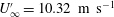 $U_{\infty }^{\prime }=10.32~\text{m}~\text{s}^{-1}$
with critical wavelength
$U_{\infty }^{\prime }=10.32~\text{m}~\text{s}^{-1}$
with critical wavelength
 $\unicode[STIX]{x1D706}^{\prime }=0.0044~\text{m}$
as determined using the potential flow theory of Carpenter & Garrad (Reference Carpenter and Garrad1986). The wall length (0.04 m) is chosen so that it is substantially longer than both this critical wavelength and that of TWF predicted by local stability theory and shown later. Accordingly, the FSI system features the dynamics of an infinitely long compliant coating most often studied in stability analyses; however, its fixed ends remain crucial in the global stability analysis presented in § 3.1.1.
$\unicode[STIX]{x1D706}^{\prime }=0.0044~\text{m}$
as determined using the potential flow theory of Carpenter & Garrad (Reference Carpenter and Garrad1986). The wall length (0.04 m) is chosen so that it is substantially longer than both this critical wavelength and that of TWF predicted by local stability theory and shown later. Accordingly, the FSI system features the dynamics of an infinitely long compliant coating most often studied in stability analyses; however, its fixed ends remain crucial in the global stability analysis presented in § 3.1.1.
Wall-2 is chosen so that the frequencies of its in vacuo structural modes in vertical displacements,
 $$\begin{eqnarray}\displaystyle \unicode[STIX]{x1D714}_{n}=\left(\frac{C_{B}(n\unicode[STIX]{x03C0}/L_{c})^{4}+C_{K}}{C_{I}}-\frac{C_{D_{z}}^{2}}{4C_{I}^{2}}\right)^{1/2}, & & \displaystyle\end{eqnarray}$$
where
 $n$
is the mode number, are close to those of the range of unstable TSWs in the boundary layer when the panel has length 0.04 m. Using the finite wall potential flow analysis of Garrad & Carpenter (Reference Garrad and Carpenter1982), divergence onset occurs at the critical flow speed
$n$
is the mode number, are close to those of the range of unstable TSWs in the boundary layer when the panel has length 0.04 m. Using the finite wall potential flow analysis of Garrad & Carpenter (Reference Garrad and Carpenter1982), divergence onset occurs at the critical flow speed
 $U_{\infty }^{\prime }=13.67~\text{m}~\text{s}^{-1}$
in the fundamental panel mode,
$U_{\infty }^{\prime }=13.67~\text{m}~\text{s}^{-1}$
in the fundamental panel mode,
 $n=1$
. Because the contribution of its flexural rigidity to overall wall stiffness far exceeds that of its spring foundation, its dynamics are very similar to those of a simple flexible plate (panel) for which the wavelength of the lowest-frequency mode is determined by the panel length. Wall-3 is of a similar type to wall-1 but it has been made stiffer so that the FSI system is free of the TWF instability and its structural eigenfrequencies are beyond the range of those of unstable TSWs while its divergence-onset flow speed is
$n=1$
. Because the contribution of its flexural rigidity to overall wall stiffness far exceeds that of its spring foundation, its dynamics are very similar to those of a simple flexible plate (panel) for which the wavelength of the lowest-frequency mode is determined by the panel length. Wall-3 is of a similar type to wall-1 but it has been made stiffer so that the FSI system is free of the TWF instability and its structural eigenfrequencies are beyond the range of those of unstable TSWs while its divergence-onset flow speed is
 $U_{\infty }^{\prime }=22.8~\text{m}~\text{s}^{-1}$
and the wavelength of the critical mode is
$U_{\infty }^{\prime }=22.8~\text{m}~\text{s}^{-1}$
and the wavelength of the critical mode is
 $\unicode[STIX]{x1D706}^{\prime }=0.008~\text{m}$
. For all walls, the effect of structural damping,
$\unicode[STIX]{x1D706}^{\prime }=0.008~\text{m}$
. For all walls, the effect of structural damping,
 $D_{z}^{\prime }$
, in the range
$D_{z}^{\prime }$
, in the range
 $0{-}10^{4}~\text{Ns}~\text{m}^{-3}$
, is studied in order to assess this as a means to control system instabilities or reduce transient growth.
$0{-}10^{4}~\text{Ns}~\text{m}^{-3}$
, is studied in order to assess this as a means to control system instabilities or reduce transient growth.
Table 1. Base values of the physical properties and non-dimensional parameters of the systems studied.

a Values for transient analysis using wall-1 physical data.
Validations of predicted eigenvalues and their corresponding eigen-vectors using the present modelling have been undertaken using appropriate comparisons with local stability analyses in the literature, for example Carpenter & Morris (Reference Carpenter and Morris1990). Our local stability results have then been used to construct the spatial amplification of convectively unstable TSWs over a compliant panel in order to create benchmarks against which the spatial amplification computed using the present methods have been compared.

Figure 2. (a) Eigenvalue spectrum at
 $Re_{s}=3000$
from global stability analysis for wall-1 data and rigid wall at
$Re_{s}=3000$
from global stability analysis for wall-1 data and rigid wall at
 $x_{s}=1012$
and frequency of the inlet boundary condition
$x_{s}=1012$
and frequency of the inlet boundary condition
 $\unicode[STIX]{x1D714}_{s}=0.07755$
, (b) detail from (a) to show the M
$\unicode[STIX]{x1D714}_{s}=0.07755$
, (b) detail from (a) to show the M
 $_{5}$
branch and its variation for different structural damping and stiffness. (The meanings of the mode branch labels M
$_{5}$
branch and its variation for different structural damping and stiffness. (The meanings of the mode branch labels M
 $_{1}$
–M
$_{1}$
–M
 $_{5}$
are provided in the text.)
$_{5}$
are provided in the text.)
Figure 2(a) shows the full eigenvalue spectrum using the wall-1 data while the detail of figure 2(b) shows the effect of two variations from the base data that increase the structural stiffness or incorporates structural damping. The horizontal axis,
 $\unicode[STIX]{x1D714}_{r}$
, gives the oscillatory part of each mode, while the vertical axis,
$\unicode[STIX]{x1D714}_{r}$
, gives the oscillatory part of each mode, while the vertical axis,
 $\unicode[STIX]{x1D714}_{i}$
gives its temporal growth rate, positive values indicating amplification while negative values indicate decay. Convergence of the global spectrum was achieved (for example, see Tsigklifis & Lucey Reference Tsigklifis and Lucey2015) with 240 uniformly distributed grid points in the streamwise direction and 75 collocation points in the vertical direction for height of the computational domain
$\unicode[STIX]{x1D714}_{i}$
gives its temporal growth rate, positive values indicating amplification while negative values indicate decay. Convergence of the global spectrum was achieved (for example, see Tsigklifis & Lucey Reference Tsigklifis and Lucey2015) with 240 uniformly distributed grid points in the streamwise direction and 75 collocation points in the vertical direction for height of the computational domain
 $L_{H}=30$
. In the streamwise discretisation, 160 points were used for the compliant wall section giving a dimensionless element length
$L_{H}=30$
. In the streamwise discretisation, 160 points were used for the compliant wall section giving a dimensionless element length
 $\unicode[STIX]{x0394}x=0.6$
, which is sufficient to resolve the wavelength of the most unstable TWF mode (17 grid points) and of the associated structural mode (13 grid points) predicted by local stability analysis. Five mode types are identified in this figure: M
$\unicode[STIX]{x0394}x=0.6$
, which is sufficient to resolve the wavelength of the most unstable TWF mode (17 grid points) and of the associated structural mode (13 grid points) predicted by local stability analysis. Five mode types are identified in this figure: M
 $_{1}$
is the TSW branch that for these system properties is seen to be stable, M
$_{1}$
is the TSW branch that for these system properties is seen to be stable, M
 $_{2}$
is the Orr mode branch, M
$_{2}$
is the Orr mode branch, M
 $_{3}$
is the continuous spectrum of the Orr–Sommerfeld equation while M
$_{3}$
is the continuous spectrum of the Orr–Sommerfeld equation while M
 $_{4}$
are modes associated with the Orr–Sommerfeld entry boundary conditions. It is noted that all of these branches can be identified with the corresponding spectrum for a rigid wall that is also plotted in figure 2(a). The fifth, M
$_{4}$
are modes associated with the Orr–Sommerfeld entry boundary conditions. It is noted that all of these branches can be identified with the corresponding spectrum for a rigid wall that is also plotted in figure 2(a). The fifth, M
 $_{5}$
, is the TWF branch that is seen to be unstable over a range of oscillation frequencies. Clearly, there is no rigid wall analogue for this flexible-wall-based mode in figure 2(a). However, it is seen in figure 2(b) that either a suitable amount of stiffening or the inclusion of sufficient structural damping stabilises the TWF branch. Finally, we have varied both the length of the rigid wall regions upstream and downstream of the compliant panel and the choice of inlet and outlet disturbance frequencies to the flow domain, used to generate complex
$_{5}$
, is the TWF branch that is seen to be unstable over a range of oscillation frequencies. Clearly, there is no rigid wall analogue for this flexible-wall-based mode in figure 2(a). However, it is seen in figure 2(b) that either a suitable amount of stiffening or the inclusion of sufficient structural damping stabilises the TWF branch. Finally, we have varied both the length of the rigid wall regions upstream and downstream of the compliant panel and the choice of inlet and outlet disturbance frequencies to the flow domain, used to generate complex
 $\unicode[STIX]{x1D6FC}$
in (2.6a,b
) to ensure that this type of modal interaction behaviour is not an artefact of the finite computational domain.
$\unicode[STIX]{x1D6FC}$
in (2.6a,b
) to ensure that this type of modal interaction behaviour is not an artefact of the finite computational domain.
3.1 Stability analysis
Herein we present predictions of the time-asymptotic behaviour of the system (i.e. solutions of the boundary-value problem) that characterise the system state after transient responses to the initiation of system disturbances have either been wholly attenuated or convected away from the region of the compliant panel. The main focus is upon the findings of the global stability analysis arising from the decomposition of (2.15) that leads to the eigen-problem of (2.16). However, we also perform local analyses wherein all perturbations are proportional to
 $\exp [\text{i}(\unicode[STIX]{x1D6FC}x-\unicode[STIX]{x1D714}t)]$
in which
$\exp [\text{i}(\unicode[STIX]{x1D6FC}x-\unicode[STIX]{x1D714}t)]$
in which
 $\unicode[STIX]{x1D6FC}=\unicode[STIX]{x1D6FC}_{r}+\text{i}\unicode[STIX]{x1D6FC}_{i}$
is the complex wavenumber that arises from solving the Orr–Sommerfeld equation (A 2), for a given frequency
$\unicode[STIX]{x1D6FC}=\unicode[STIX]{x1D6FC}_{r}+\text{i}\unicode[STIX]{x1D6FC}_{i}$
is the complex wavenumber that arises from solving the Orr–Sommerfeld equation (A 2), for a given frequency
 $\unicode[STIX]{x1D714}$
. Clearly this type of analysis uses the assumption of a compliant panel that is infinitely long within a boundary layer of fixed displacement thickness determined by the value of the local Reynolds number at the mid-chord of the panel, and its formulation only permits spatial growth or decay (
$\unicode[STIX]{x1D714}$
. Clearly this type of analysis uses the assumption of a compliant panel that is infinitely long within a boundary layer of fixed displacement thickness determined by the value of the local Reynolds number at the mid-chord of the panel, and its formulation only permits spatial growth or decay (
 $\unicode[STIX]{x1D6FC}_{i}<0$
and
$\unicode[STIX]{x1D6FC}_{i}<0$
and
 $\unicode[STIX]{x1D6FC}_{i}>0$
respectively, for downstream-propagating modes) of system disturbances.
$\unicode[STIX]{x1D6FC}_{i}>0$
respectively, for downstream-propagating modes) of system disturbances.
3.1.1 Travelling wave flutter branch
Using local analyses, TWF on a compliant wall of infinite extent has been shown to be a convective instability (Carpenter & Garrad Reference Carpenter and Garrad1986; Carpenter & Morris Reference Carpenter and Morris1990; Dixon et al. Reference Dixon, Lucey and Carpenter1994; Lucey & Carpenter Reference Lucey and Carpenter1995). For the definition of convective and absolute instabilities, see Huerre & Monkewitz (Reference Huerre and Monkewitz1985, Reference Huerre and Monkewitz1990), while Lucey (Reference Lucey1998), Lucey & Peake (Reference Lucey, Peake, Carpenter and Pedley2003) describe the application of these concepts when ideal flow interacts with a flexible panel. Unstable TWF waves grow spatially in the downstream direction from a source of applied excitation. The instability arises from the action of the fluid flow on what are essentially structural waves, their growth caused by irreversible transfer of energy from the flow to the flexible wall that occurs when a critical layer exists within the boundary layer. In the wave classification system of Benjamin (Reference Benjamin1963), they are denoted Class B.

Figure 3. Spatio-temporal evolution of the panel deflection for the most unstable global mode on the TWF branch (M
 $_{5}$
) in figure 2. The dashed and dotted lines are plots of the spatial amplification of the structural (S) and TWF modes found using a local stability analysis at the global mode frequency and shown in figure 5(a) positioned as a best fit to the global mode. The computational domain extends from
$_{5}$
) in figure 2. The dashed and dotted lines are plots of the spatial amplification of the structural (S) and TWF modes found using a local stability analysis at the global mode frequency and shown in figure 5(a) positioned as a best fit to the global mode. The computational domain extends from
 $x=1012$
–1158 (non-dimensional distances from the boundary-layer origin) while the compliant panel occupies the region
$x=1012$
–1158 (non-dimensional distances from the boundary-layer origin) while the compliant panel occupies the region
 $x=1037$
–1134.
$x=1037$
–1134.
For a finite panel with wall-1 data, figure 2 (see branch M
 $_{5}$
) shows that TWF can become a global, temporally amplifying, instability that would lead to the destabilisation of the compliant panel at all spatial locations and without a continuing applied source of excitation. We emphasise that the global temporal amplification of this unstable branch is insensitive to changes of the inlet outlet boundary conditions nor increases to the length of the compliant panel. To understand the global destabilisation mechanism, we present in figure 3 the time evolution of the panel deflection for the most unstable TWF branch eigenvalue in figure 2. First, it is clearly seen that the amplitude of the mode grows with time
$_{5}$
) shows that TWF can become a global, temporally amplifying, instability that would lead to the destabilisation of the compliant panel at all spatial locations and without a continuing applied source of excitation. We emphasise that the global temporal amplification of this unstable branch is insensitive to changes of the inlet outlet boundary conditions nor increases to the length of the compliant panel. To understand the global destabilisation mechanism, we present in figure 3 the time evolution of the panel deflection for the most unstable TWF branch eigenvalue in figure 2. First, it is clearly seen that the amplitude of the mode grows with time
 $t$
(non-dimensionalised using displacement thickness and free-stream flow speed). Second, is also seen to be spatially amplified by comparing deflection amplitudes near the compliant panel leading edge (
$t$
(non-dimensionalised using displacement thickness and free-stream flow speed). Second, is also seen to be spatially amplified by comparing deflection amplitudes near the compliant panel leading edge (
 $x=1040$
where the coordinate of location is non-dimensionalised using the displacement thickness) with those near its trailing edge (
$x=1040$
where the coordinate of location is non-dimensionalised using the displacement thickness) with those near its trailing edge (
 $x=1130$
). The dashed and dotted line envelopes in these figures signify the spatial change in amplitude of the structural (S) and TWF mode respectively predicted by local stability analysis conducted at the complex frequency of the global mode, the results of which are presented in figure 5(a) that will be discussed later. It can be seen that the spatial amplification of the wall displacement in the downstream direction predicted by the global model agrees well with that of the structural mode predicted by a local stability analysis; however, the structural mode is spatially stabilised in the direction of its phase speed and group speed. The spatial amplification of the velocity disturbance away from the wall predicted by the global stability agrees with that of the TWF mode predicted by a local stability analysis (not shown). Finally, it can be seen that the global mode is a combination of two types of wave, the expected downstream-travelling TWF (predicted by a local stability analysis) and an upstream-travelling wave. It is this combination of waves on a flexible wall with fixed ends, permitting energy propagation in both downstream and upstream directions, that leads to the temporal growth found for the global mode. The TWF transfers flow kinetic energy to the compliant wall as it propagates downstream. At the trailing edge the TWF continuously excites the upstream-propagating structural mode and its arrival at the leading edge of the compliant panel provides a continuous source of excitation for the TWF.
$x=1130$
). The dashed and dotted line envelopes in these figures signify the spatial change in amplitude of the structural (S) and TWF mode respectively predicted by local stability analysis conducted at the complex frequency of the global mode, the results of which are presented in figure 5(a) that will be discussed later. It can be seen that the spatial amplification of the wall displacement in the downstream direction predicted by the global model agrees well with that of the structural mode predicted by a local stability analysis; however, the structural mode is spatially stabilised in the direction of its phase speed and group speed. The spatial amplification of the velocity disturbance away from the wall predicted by the global stability agrees with that of the TWF mode predicted by a local stability analysis (not shown). Finally, it can be seen that the global mode is a combination of two types of wave, the expected downstream-travelling TWF (predicted by a local stability analysis) and an upstream-travelling wave. It is this combination of waves on a flexible wall with fixed ends, permitting energy propagation in both downstream and upstream directions, that leads to the temporal growth found for the global mode. The TWF transfers flow kinetic energy to the compliant wall as it propagates downstream. At the trailing edge the TWF continuously excites the upstream-propagating structural mode and its arrival at the leading edge of the compliant panel provides a continuous source of excitation for the TWF.
As has been seen in figure 2 the inclusion of sufficient structural damping
 $C_{D_{z}}$
stabilises the TWF branch. This might be expected since TWF occurs essentially through the destabilisation of what is a wall flexural wave (that exists in vacuo) and it has been categorised as a Class B wave. Stiffening the compliant panel by increasing the spring stiffness
$C_{D_{z}}$
stabilises the TWF branch. This might be expected since TWF occurs essentially through the destabilisation of what is a wall flexural wave (that exists in vacuo) and it has been categorised as a Class B wave. Stiffening the compliant panel by increasing the spring stiffness
 $C_{K}$
also exercises a stabilising effect as evidenced in the same figure. Again, this could have been anticipated on the basis of local stability analyses, given that in the limit of infinite stiffness the wall is rigid and therefore unable to support the flexural waves that are the source of TWF; in fact, when the compliant coating is sufficiently stiff that the speed of its structural waves exceeds that of the free-stream flow (external to the boundary layer) the critical layer ceases to exist.
$C_{K}$
also exercises a stabilising effect as evidenced in the same figure. Again, this could have been anticipated on the basis of local stability analyses, given that in the limit of infinite stiffness the wall is rigid and therefore unable to support the flexural waves that are the source of TWF; in fact, when the compliant coating is sufficiently stiff that the speed of its structural waves exceeds that of the free-stream flow (external to the boundary layer) the critical layer ceases to exist.
We now consider the effect of the Reynolds number on the global TWF mode instability. Figure 4 shows its temporal amplification curves in the
 $\unicode[STIX]{x1D714}_{r}$
–
$\unicode[STIX]{x1D714}_{r}$
–
 $Re_{s}$
plane as predicted by the global stability analysis. For comparison, we have also included the neutral curve predicted by our local spatial stability analysis. There is a good match between local spatial and global temporal stability regarding the prediction of the critical Reynolds number – the value at which instability first appears with increasing
$Re_{s}$
plane as predicted by the global stability analysis. For comparison, we have also included the neutral curve predicted by our local spatial stability analysis. There is a good match between local spatial and global temporal stability regarding the prediction of the critical Reynolds number – the value at which instability first appears with increasing
 $Re_{s}$
– and the lower part of the neutral curve but poor agreement for the upper branch. As can be discerned in figure 2 when damping is absent, the TWF branch (M
$Re_{s}$
– and the lower part of the neutral curve but poor agreement for the upper branch. As can be discerned in figure 2 when damping is absent, the TWF branch (M
 $_{5}$
) crosses the real axis as a near asymptote that gives large values of the oscillatory frequency
$_{5}$
) crosses the real axis as a near asymptote that gives large values of the oscillatory frequency
 $\unicode[STIX]{x1D714}_{r}$
which correspond to small spatial wavelength. The global stability model is stretched to resolve accurately the small spatial wavelength spectrum due to the use of a second-order finite-difference scheme for streamwise spatial discretisation. However, the discretisation parameters we have used accurately capture the eigenvalues of the main instability loop and the maximum temporal amplification rate because these are located at lower oscillation frequencies.
$\unicode[STIX]{x1D714}_{r}$
which correspond to small spatial wavelength. The global stability model is stretched to resolve accurately the small spatial wavelength spectrum due to the use of a second-order finite-difference scheme for streamwise spatial discretisation. However, the discretisation parameters we have used accurately capture the eigenvalues of the main instability loop and the maximum temporal amplification rate because these are located at lower oscillation frequencies.

Figure 4. Temporal amplification curves in the
 $\unicode[STIX]{x1D714}_{r}$
–
$\unicode[STIX]{x1D714}_{r}$
–
 $Re_{s}$
plane for the TWF mode predicted by the global stability analysis for wall-1 data at
$Re_{s}$
plane for the TWF mode predicted by the global stability analysis for wall-1 data at
 $x_{s}^{\prime }=0.416$
m with
$x_{s}^{\prime }=0.416$
m with
 $Re_{s}$
varied through the free-stream flow speed. The neutral curve predicted by local spatial stability analysis is also included.
$Re_{s}$
varied through the free-stream flow speed. The neutral curve predicted by local spatial stability analysis is also included.
We now show how the foregoing globally unstable TWF mode branch might manifest itself in a local stability analysis. Figures 5(a) and 5(b) are dispersion diagrams, without and with (at
 $C_{D_{z}}=0.2$
) structural damping, respectively, for wavenumber as a function of real wave frequency; i.e. the results of a spatial stability analysis. The local analysis is conducted for the Reynolds number obtained using the displacement thickness at the mid-point of the compliant panel. In these figures the real part of the eigenvalue,
$C_{D_{z}}=0.2$
) structural damping, respectively, for wavenumber as a function of real wave frequency; i.e. the results of a spatial stability analysis. The local analysis is conducted for the Reynolds number obtained using the displacement thickness at the mid-point of the compliant panel. In these figures the real part of the eigenvalue,
 $\unicode[STIX]{x1D6FC}_{r}$
, indicating the inverse of wavelength, is plotted as different types of blue lines for the different mode branches with axis scale on the left of the figure. The imaginary part of each eigenvalue,
$\unicode[STIX]{x1D6FC}_{r}$
, indicating the inverse of wavelength, is plotted as different types of blue lines for the different mode branches with axis scale on the left of the figure. The imaginary part of each eigenvalue,
 $\unicode[STIX]{x1D6FC}_{i}$
, that gives the spatial amplification is plotted in red with its axis scale in red on the right of the figure. For a downstream-propagating wave, spatial amplification and decay in the downstream direction are respectively indicated by negative and positive values of
$\unicode[STIX]{x1D6FC}_{i}$
, that gives the spatial amplification is plotted in red with its axis scale in red on the right of the figure. For a downstream-propagating wave, spatial amplification and decay in the downstream direction are respectively indicated by negative and positive values of
 $\unicode[STIX]{x1D6FC}_{i}$
; for upstream-propagating waves, positive and negative values indicate amplification and decay respectively in the upstream direction. The direction of wave travel can be inferred from the wave phase speed,
$\unicode[STIX]{x1D6FC}_{i}$
; for upstream-propagating waves, positive and negative values indicate amplification and decay respectively in the upstream direction. The direction of wave travel can be inferred from the wave phase speed,
 $c=\unicode[STIX]{x1D714}_{r}/\unicode[STIX]{x1D6FC}_{r}$
and propagation from the sign of group velocity (
$c=\unicode[STIX]{x1D714}_{r}/\unicode[STIX]{x1D6FC}_{r}$
and propagation from the sign of group velocity (
 $c_{g}=\unicode[STIX]{x2202}\unicode[STIX]{x1D714}_{r}/\unicode[STIX]{x2202}\unicode[STIX]{x1D6FC}_{r}$
). We have also included the in vacuo dispersion curve for the compliant wall because it is readily seen that the TWF and S mode branches respectively approach those of the downstream and upstream free waves of the wall as the effect of fluid loading steadily reduces with increasing frequency. The different types of blue (real part) and red (imaginary part) markers added into the figures are the complex wavenumbers that result when the complex frequency
$c_{g}=\unicode[STIX]{x2202}\unicode[STIX]{x1D714}_{r}/\unicode[STIX]{x2202}\unicode[STIX]{x1D6FC}_{r}$
). We have also included the in vacuo dispersion curve for the compliant wall because it is readily seen that the TWF and S mode branches respectively approach those of the downstream and upstream free waves of the wall as the effect of fluid loading steadily reduces with increasing frequency. The different types of blue (real part) and red (imaginary part) markers added into the figures are the complex wavenumbers that result when the complex frequency
 $\unicode[STIX]{x1D714}=\unicode[STIX]{x1D714}_{r}+\text{i}\unicode[STIX]{x1D714}_{i}$
of the most unstable global mode on the TWF branch (M
$\unicode[STIX]{x1D714}=\unicode[STIX]{x1D714}_{r}+\text{i}\unicode[STIX]{x1D714}_{i}$
of the most unstable global mode on the TWF branch (M
 $_{5}$
) and the least stable global mode on the TSW branch (M
$_{5}$
) and the least stable global mode on the TSW branch (M
 $_{1}$
) in figure 2 are used in the local analysis.
$_{1}$
) in figure 2 are used in the local analysis.
In figure 5(a) the local stability analysis reveals the expected downstream-propagating (with positive
 $\unicode[STIX]{x1D6FC}_{r}$
) TWF branch that amplifies in the downstream direction. Also evident is the upstream-propagating (with negative
$\unicode[STIX]{x1D6FC}_{r}$
) TWF branch that amplifies in the downstream direction. Also evident is the upstream-propagating (with negative
 $\unicode[STIX]{x1D6FC}_{r}$
) structural mode branch labelled S that evidences wave travel and attenuation in the upstream direction. These features could be demonstrated formally through the Briggs–Bers technique (for its application to potential flow over a flexible wall see Peake Reference Peake2004) or in the analytical categorisation of wave types in Ashpis & Reshotko (Reference Ashpis and Reshotko1990) as (ci) in their figure 5 with the compliant panel trailing edge acting as its source of excitation in the global stability analysis. Thus, the global mode that contained two wave types in figure 3 may be considered to be the combined effect of these two modes predicted by the local analysis. However, a local analysis alone would not be sufficient to show that these combine to yield a global instability on a panel of finite extent. Moreover, while the wavelengths of these two modes at the complex frequency of the global mode are predicted well by the local stability analysis, their amplification/decay rates are not; in fact it can be seen that the local stability analysis overpredicts the downstream amplification of the TWF mode while it underpredicts the upstream attenuation of the structural mode. Accordingly, we may conclude that while the local stability analysis can provide the basis for understanding the interaction of finite compliant panels with a boundary-layer flow, only a global analysis can yield quantitative predictions of system stability. Figure 5(b) shows that structural damping levels, sufficient to stabilise the global TWF mode branch (see figure 2
b), do not eliminate the spatial amplification of the TWF mode branch that continues to exist as a convectively unstable mode, albeit with reduced spatial growth rate (comparison of red continuous lines between figures 5
a and 5
b). However, the local stability analysis at the frequency of the most unstable global TWF modes in figure 2 with and without damping predicts only a slight stabilisation of the spatial amplification (comparison of the red triangles between figures 5
a and 5
b). Structural damping is also seen to increase the attenuation of the upstream-travelling structural wave in its direction of propagation and this reinforces the interpretation of the global TWF mode instability of a finite panel as comprising a combination of the TWF and S modes predicted by local stability analyses.
$\unicode[STIX]{x1D6FC}_{r}$
) structural mode branch labelled S that evidences wave travel and attenuation in the upstream direction. These features could be demonstrated formally through the Briggs–Bers technique (for its application to potential flow over a flexible wall see Peake Reference Peake2004) or in the analytical categorisation of wave types in Ashpis & Reshotko (Reference Ashpis and Reshotko1990) as (ci) in their figure 5 with the compliant panel trailing edge acting as its source of excitation in the global stability analysis. Thus, the global mode that contained two wave types in figure 3 may be considered to be the combined effect of these two modes predicted by the local analysis. However, a local analysis alone would not be sufficient to show that these combine to yield a global instability on a panel of finite extent. Moreover, while the wavelengths of these two modes at the complex frequency of the global mode are predicted well by the local stability analysis, their amplification/decay rates are not; in fact it can be seen that the local stability analysis overpredicts the downstream amplification of the TWF mode while it underpredicts the upstream attenuation of the structural mode. Accordingly, we may conclude that while the local stability analysis can provide the basis for understanding the interaction of finite compliant panels with a boundary-layer flow, only a global analysis can yield quantitative predictions of system stability. Figure 5(b) shows that structural damping levels, sufficient to stabilise the global TWF mode branch (see figure 2
b), do not eliminate the spatial amplification of the TWF mode branch that continues to exist as a convectively unstable mode, albeit with reduced spatial growth rate (comparison of red continuous lines between figures 5
a and 5
b). However, the local stability analysis at the frequency of the most unstable global TWF modes in figure 2 with and without damping predicts only a slight stabilisation of the spatial amplification (comparison of the red triangles between figures 5
a and 5
b). Structural damping is also seen to increase the attenuation of the upstream-travelling structural wave in its direction of propagation and this reinforces the interpretation of the global TWF mode instability of a finite panel as comprising a combination of the TWF and S modes predicted by local stability analyses.

Figure 5. Dispersion diagrams showing the variation of complex wavenumber, with real (blue) and imaginary (red) parts respectively on left and right vertical axes, with wave frequency for (a)
 $C_{D_{z}}=0$
and (b)
$C_{D_{z}}=0$
and (b)
 $C_{D_{z}}=0.2$
. Discrete data markers indicate the complex eigenvalues from the local stability analysis conducted at the complex frequencies of the most unstable TWF global mode (triangles and circles respectively for TWF and S modes) and the least stable global TSW mode (crosses and squares respectively for compliant and rigid walls) of figure 2. The grey line is the dispersion curve for free waves of the compliant wall.
$C_{D_{z}}=0.2$
. Discrete data markers indicate the complex eigenvalues from the local stability analysis conducted at the complex frequencies of the most unstable TWF global mode (triangles and circles respectively for TWF and S modes) and the least stable global TSW mode (crosses and squares respectively for compliant and rigid walls) of figure 2. The grey line is the dispersion curve for free waves of the compliant wall.
Turning attention to the globally stable TSW branch in figure 2, it is seen in figure 5(a) that there exists a range of frequencies for which TSWs are convectively unstable in that they amplify as they propagate downstream. The local analysis conducted at the complex frequency of the least stable global mode shows (see markers) that a conventional local stability analysis underpredicts the growth rate of the unstable mode. It is also seen by comparing the growth rates of the TSW markers that wall compliance has a mildly stabilising effect on the convectively unstable TSWs as compared with their amplification over a rigid wall (comparison of the red crosses and squares in figure 5 a). Comparing figures 5(a) and 5(b), the spatial growth rate of the TSW is also seen to be slightly increased by the inclusion of damping but the compliant panel continues to exercise a stabilising effect on the TSW as compared to its growth over a rigid wall.
Comparing the spatial amplification rates of the most unstable TWF and TSW modes, either for real
 $\unicode[STIX]{x1D714}$
or the global complex
$\unicode[STIX]{x1D714}$
or the global complex
 $\unicode[STIX]{x1D714}$
, in figure 5(a,b), it can be seen that the amplification of the convectively unstable TWF mode is greater than the spatial amplification rate of the TSW mode and that structural damping is only marginally attenuating at the global frequency. A compliant panel with these properties could not be used for transition delay because the spatial amplification of the TWF mode exceeds that of TSW and thus it may be TWF that causes transition as has been shown to occur by Lucey & Carpenter (Reference Lucey and Carpenter1995) when modelling the experiments of Gaster (Reference Gaster, Liepmann and Narasimha1988). Accordingly, in practical applications of compliant panels for transition delay it is essential to choose compliant wall properties (a combination of structural stiffness and damping for a given mass ratio
$\unicode[STIX]{x1D714}$
, in figure 5(a,b), it can be seen that the amplification of the convectively unstable TWF mode is greater than the spatial amplification rate of the TSW mode and that structural damping is only marginally attenuating at the global frequency. A compliant panel with these properties could not be used for transition delay because the spatial amplification of the TWF mode exceeds that of TSW and thus it may be TWF that causes transition as has been shown to occur by Lucey & Carpenter (Reference Lucey and Carpenter1995) when modelling the experiments of Gaster (Reference Gaster, Liepmann and Narasimha1988). Accordingly, in practical applications of compliant panels for transition delay it is essential to choose compliant wall properties (a combination of structural stiffness and damping for a given mass ratio
 $C_{I}$
) that prevent global instability and postpone the onset and/or reduce the growth rates of convectively unstable TSWs and TWF. The latter has been accomplished in the optimisation of transition delay based upon local stability analyses (Carpenter Reference Carpenter1991; Dixon et al.
Reference Dixon, Lucey and Carpenter1994). Accordingly, in what follows we focus on a parametric study of the effects of structural stiffness and damping on the stability of the global TWF mode.
$C_{I}$
) that prevent global instability and postpone the onset and/or reduce the growth rates of convectively unstable TSWs and TWF. The latter has been accomplished in the optimisation of transition delay based upon local stability analyses (Carpenter Reference Carpenter1991; Dixon et al.
Reference Dixon, Lucey and Carpenter1994). Accordingly, in what follows we focus on a parametric study of the effects of structural stiffness and damping on the stability of the global TWF mode.

Figure 6. Variation of structural stiffness at which global TWF mode instability first occurs with Reynolds number through (a) variation of the distance of the flexible panel from the boundary-layer origin for different fixed free-stream flow speed flow speeds,
 $U_{\infty }^{\prime }$
, and (b) variation of the free-stream flow speed for different fixed distances
$U_{\infty }^{\prime }$
, and (b) variation of the free-stream flow speed for different fixed distances
 $x_{s}^{\prime }$
.
$x_{s}^{\prime }$
.
We first focus upon the relationship between compliant panel stiffness and the Reynolds number at which global instability on the TWF branch first occurs. To characterise the stiffness, that comprises contributions from both plate flexure and spring foundation, we define a non-dimensional wall stiffness as the ratio of its minimum free wave speed to the free-stream flow speed, hence
 $$\begin{eqnarray}\displaystyle K_{IW}={\displaystyle \frac{c_{min}^{\prime }}{U_{\infty }^{\prime }}}={\displaystyle \frac{(4C_{K}C_{B})^{1/4}}{C_{I}^{1/2}}}. & & \displaystyle\end{eqnarray}$$
We remark that the simple inviscid theory of Carpenter & Garrad (Reference Carpenter and Garrad1986), using a local analysis, predicts
 $K_{IW}=1$
as the criterion for TWF onset on the basis that this value is the threshold between the existence and absence of a critical layer within the boundary layer.
$K_{IW}=1$
as the criterion for TWF onset on the basis that this value is the threshold between the existence and absence of a critical layer within the boundary layer.
It is well known that the self-similarity of Blasius boundary-layer flow means that its dynamics can be characterised uniquely by the Reynolds number. This continues to be the case for local stability analyses where non-parallel effects are neglected and the compliant wall is homogenous in the streamwise direction. However, when a panel of finite length is inserted in an otherwise rigid wall, the FSI system becomes inhomogeneous in the streamwise direction. Accordingly for a fluid with given kinematic viscosity, Reynolds number variation can be achieved in one of two distinct ways, either (i) changing the downstream distance of the plate
 $x_{s}^{\prime }$
(from the boundary-layer origin) for a fixed free-stream flow speed
$x_{s}^{\prime }$
(from the boundary-layer origin) for a fixed free-stream flow speed
 $U_{\infty }^{\prime }$
or (ii) changing the free-stream flow speed
$U_{\infty }^{\prime }$
or (ii) changing the free-stream flow speed
 $U_{\infty }^{\prime }$
for a fixed position
$U_{\infty }^{\prime }$
for a fixed position
 $x_{s}^{\prime }$
of the compliant panel. These changes do not give equivalent FSI dynamics even though they may result in the same Reynolds number. The former appears more appropriate for theoretical analysis because the dimensionless stiffness depends only on the structural properties, while the latter is more convenient for comparison with experimental measurements obtained at a specific location along the plate.
$x_{s}^{\prime }$
of the compliant panel. These changes do not give equivalent FSI dynamics even though they may result in the same Reynolds number. The former appears more appropriate for theoretical analysis because the dimensionless stiffness depends only on the structural properties, while the latter is more convenient for comparison with experimental measurements obtained at a specific location along the plate.

Figure 7. (a) Eigenvalue spectrum from global stability analysis for different Reynolds numbers and fixed free-stream speed
 $U_{\infty }^{\prime }=10~\text{m}~\text{s}^{-1}$
. (b) Distribution of the energy production function
$U_{\infty }^{\prime }=10~\text{m}~\text{s}^{-1}$
. (b) Distribution of the energy production function
 $S$
through the boundary layer for the cases shown in (a) produced by local stability analysis using wall-1 properties.
$S$
through the boundary layer for the cases shown in (a) produced by local stability analysis using wall-1 properties.
In figure 6(a) we show how the stiffness
 $K_{IW}$
at which global TWF mode instability first appears varies with the Reynolds number for different values of a fixed free-stream flow speed
$K_{IW}$
at which global TWF mode instability first appears varies with the Reynolds number for different values of a fixed free-stream flow speed
 $U_{\infty }^{\prime }$
where the streamwise position,
$U_{\infty }^{\prime }$
where the streamwise position,
 $x_{s}^{\prime }$
(hence boundary-layer thickness), is varied. Figure 6(b) is the corresponding result but here the flow speed is allowed to vary while different fixed downstream positions
$x_{s}^{\prime }$
(hence boundary-layer thickness), is varied. Figure 6(b) is the corresponding result but here the flow speed is allowed to vary while different fixed downstream positions
 $x_{s}^{\prime }$
are considered. These results have been generated using the local spatial stability analysis and have been verified a posteriori with the global stability, since, as can be seen in figure 4, there is good agreement between local and global stability analyses for the lower branch of the neutral curve and the lowest Reynolds number at which the global TWF branch features instability. These results indicate that the FSI system becomes more stable with respect to global TWF modes with increasing downstream distance from the leading edge of the plate at a given free-stream flow speed
$x_{s}^{\prime }$
are considered. These results have been generated using the local spatial stability analysis and have been verified a posteriori with the global stability, since, as can be seen in figure 4, there is good agreement between local and global stability analyses for the lower branch of the neutral curve and the lowest Reynolds number at which the global TWF branch features instability. These results indicate that the FSI system becomes more stable with respect to global TWF modes with increasing downstream distance from the leading edge of the plate at a given free-stream flow speed
 $U_{\infty }^{\prime }$
, or as the free-stream flow speed increases for a given position of the plate. Moreover, figure 6(a) shows that, at any given location of the flexible panel, a higher flow speed is destabilising and this can be expected since the ratio of wall stiffness to flow stiffness (that scales with the dynamic pressure of the free-stream flow) is reduced; i.e. the wall appears softer. Figure 6(b) shows that, for any given flow speed, the flexible panel is more stable when located further downstream where the boundary layer is thicker via higher
$U_{\infty }^{\prime }$
, or as the free-stream flow speed increases for a given position of the plate. Moreover, figure 6(a) shows that, at any given location of the flexible panel, a higher flow speed is destabilising and this can be expected since the ratio of wall stiffness to flow stiffness (that scales with the dynamic pressure of the free-stream flow) is reduced; i.e. the wall appears softer. Figure 6(b) shows that, for any given flow speed, the flexible panel is more stable when located further downstream where the boundary layer is thicker via higher
 $x_{s}^{\prime }$
and/or lower Reynolds number (free-stream flow speed for the variation used in figure 6
b). It is noted that
$x_{s}^{\prime }$
and/or lower Reynolds number (free-stream flow speed for the variation used in figure 6
b). It is noted that
 $K_{IW}$
can exceed unity but this does not mean that the critical layer does not exist. The approximate threshold
$K_{IW}$
can exceed unity but this does not mean that the critical layer does not exist. The approximate threshold
 $K_{IW}=1$
discussed below (3.2) above is based upon the assumption of a thin boundary layer and its formulation does not account for the effects of fluid inertia on the compliant wall wave speed.
$K_{IW}=1$
discussed below (3.2) above is based upon the assumption of a thin boundary layer and its formulation does not account for the effects of fluid inertia on the compliant wall wave speed.
Figure 7(a) confirms the finding that the FSI system becomes more stable with increased downstream location of the flexible panel for a given free-stream flow speed
 $U_{\infty }^{\prime }$
. In this figure we plot the temporal eigenvalue spectrum from the global stability analysis for different Reynolds numbers while maintaining a constant free-stream flow speed
$U_{\infty }^{\prime }$
. In this figure we plot the temporal eigenvalue spectrum from the global stability analysis for different Reynolds numbers while maintaining a constant free-stream flow speed
 $U_{\infty }^{\prime }=10~\text{m}~\text{s}^{-1}$
. The temporal growth rates of the TWF modes reduce with increasing downstream location because the wavelength of the instability becomes smaller relative to the length of the compliant wall and therefore the finiteness effect of the compliant panel that underpins the global instability is reduced.
$U_{\infty }^{\prime }=10~\text{m}~\text{s}^{-1}$
. The temporal growth rates of the TWF modes reduce with increasing downstream location because the wavelength of the instability becomes smaller relative to the length of the compliant wall and therefore the finiteness effect of the compliant panel that underpins the global instability is reduced.
The principal mechanism of the TWF instability is the phase shift in the pressure perturbation across the critical layer which gives rise to irreversible energy transfer to the wall (Carpenter & Gajjar Reference Carpenter and Gajjar1990; Carpenter & Morris Reference Carpenter and Morris1990). In order to reveal why increasing the downstream distance of the flexible panel from the origin of the boundary layer is stabilising for the global TWF mode, we use a local stability analysis to calculate the rate of work done by the pressure disturbance on the wall (Carpenter & Morris Reference Carpenter and Morris1990),
 $$\begin{eqnarray}p{\displaystyle \frac{\unicode[STIX]{x2202}\unicode[STIX]{x1D702}_{z}}{\unicode[STIX]{x2202}t}}\sim \int _{0}^{L_{H}}\text{Re}\left[\left(\text{i}(\unicode[STIX]{x1D6FC}U_{x}-\unicode[STIX]{x1D714})\hat{u} _{z}-{\displaystyle \frac{1}{Re_{x}}}\left({\displaystyle \frac{\text{d}^{2}}{\text{d}z^{2}}}-\unicode[STIX]{x1D6FC}^{2}\right)\hat{u} _{z}\right)\hat{u} _{z}(H=0)\right]\text{d}H=\int _{0}^{L_{H}}S\,\text{d}H,\end{eqnarray}$$
having integrated the
 $z$
-component of linearised Navier–Stokes equations from the compliant wall through to the free stream to obtain the pressure perturbation on the wall. Figure 7(b) shows the distribution of the function
$z$
-component of linearised Navier–Stokes equations from the compliant wall through to the free stream to obtain the pressure perturbation on the wall. Figure 7(b) shows the distribution of the function
 $S$
through the boundary layer for the cases shown in figure 7(a). It can be seen that as the boundary layer progresses downstream both the positive rate of work above the critical layer and the dissipation in the viscous wall layer become smaller in magnitude but the total contribution is in favour of the global TWF mode stabilisation. As the boundary layer progresses downstream, its thickness increases and the critical layer, where the fluid flow speed equals the surface wave speed, moves away from the wall and its effect is attenuated.
$S$
through the boundary layer for the cases shown in figure 7(a). It can be seen that as the boundary layer progresses downstream both the positive rate of work above the critical layer and the dissipation in the viscous wall layer become smaller in magnitude but the total contribution is in favour of the global TWF mode stabilisation. As the boundary layer progresses downstream, its thickness increases and the critical layer, where the fluid flow speed equals the surface wave speed, moves away from the wall and its effect is attenuated.

Figure 8. Variation of structural damping at which global TWF mode instability first occurs with Reynolds number using both global and local stability analyses, for different values of foundation spring stiffness (
 $K^{\prime }$
), through (a) variation of the distance of the flexible panel from the boundary-layer origin for different fixed free-stream flow speeds,
$K^{\prime }$
), through (a) variation of the distance of the flexible panel from the boundary-layer origin for different fixed free-stream flow speeds,
 $U_{\infty }^{\prime }$
, and (b) variation of the free-stream flow speed for different fixed distances
$U_{\infty }^{\prime }$
, and (b) variation of the free-stream flow speed for different fixed distances
 $x_{s}^{\prime }$
.
$x_{s}^{\prime }$
.
We now consider the effect of structural damping in conjunction with compliant wall stiffness variations. We define the non-dimensional damping, based upon the dynamics of the compliant wall in vacuo, as
 $$\begin{eqnarray}\displaystyle D_{IW}={\displaystyle \frac{D_{z}^{\prime }c_{min}^{\prime }}{\unicode[STIX]{x1D70C}_{l}^{\prime }U_{\infty }^{^{\prime }2}}}={\displaystyle \frac{C_{D_{z}}(-C_{D_{z}}^{2}+4C_{I}C_{K})^{1/4}C_{B}^{1/4}}{C_{I}^{3/4}}}, & & \displaystyle\end{eqnarray}$$
noting that the physical damping is constrained by
 $C_{D_{z}}<2\sqrt{C_{I}C_{K}}$
; i.e. lower than critical damping for the wall structure.
$C_{D_{z}}<2\sqrt{C_{I}C_{K}}$
; i.e. lower than critical damping for the wall structure.
Figures 8(a) and 8(b) plot the variation with Reynolds number of the minimum value of damping
 $D_{IW}$
required to stabilise all modes on the global TWF branch in figure 2 for different values of fixed free-stream flow speeds and fixed positions of the flexible panel plate respectively, and different values of the foundation spring stiffness. These results have been generated through the combined use of global and local stability analyses using the following procedure. For given Reynolds number and compliant wall stiffness we conduct a global stability analysis without structural damping. This result is then used to conduct a local spatial stability analysis at the predicted complex frequency
$D_{IW}$
required to stabilise all modes on the global TWF branch in figure 2 for different values of fixed free-stream flow speeds and fixed positions of the flexible panel plate respectively, and different values of the foundation spring stiffness. These results have been generated through the combined use of global and local stability analyses using the following procedure. For given Reynolds number and compliant wall stiffness we conduct a global stability analysis without structural damping. This result is then used to conduct a local spatial stability analysis at the predicted complex frequency
 $\unicode[STIX]{x1D714}=\unicode[STIX]{x1D714}_{r}+\text{i}\unicode[STIX]{x1D714}_{i}$
with the maximum temporal amplification
$\unicode[STIX]{x1D714}=\unicode[STIX]{x1D714}_{r}+\text{i}\unicode[STIX]{x1D714}_{i}$
with the maximum temporal amplification
 $\unicode[STIX]{x1D714}_{i}$
, increasing the structural damping until the spatial amplification
$\unicode[STIX]{x1D714}_{i}$
, increasing the structural damping until the spatial amplification
 $\unicode[STIX]{x1D6FC}_{i}$
crosses the real axis and becomes positive, indicating a spatially stable mode. For this value of the structural damping, we then perform the global stability analysis to verify that this value of damping marginally stabilises the TWF global instability branch. This approach has been adopted to reduce the number of computationally expensive global calculations. From the results in figure 8(a,b), it can be seen that there is a good agreement between local and global stability analyses except for cases where edge effects of the finite compliant wall are non-negligible and a higher value of structural damping is needed. Overall, figure 8(a,b) shows that the level of damping required to eliminate the global TWF mode instability reduces as the boundary layer progresses downstream or with an increase to the compliant wall stiffness and/or the decrease of the free-stream flow speed. These findings align with those of figure 6(a,b), because the global TWF instability can be stabilised by each of increased structural stiffness and damping or a combination thereof.
$\unicode[STIX]{x1D6FC}_{i}$
crosses the real axis and becomes positive, indicating a spatially stable mode. For this value of the structural damping, we then perform the global stability analysis to verify that this value of damping marginally stabilises the TWF global instability branch. This approach has been adopted to reduce the number of computationally expensive global calculations. From the results in figure 8(a,b), it can be seen that there is a good agreement between local and global stability analyses except for cases where edge effects of the finite compliant wall are non-negligible and a higher value of structural damping is needed. Overall, figure 8(a,b) shows that the level of damping required to eliminate the global TWF mode instability reduces as the boundary layer progresses downstream or with an increase to the compliant wall stiffness and/or the decrease of the free-stream flow speed. These findings align with those of figure 6(a,b), because the global TWF instability can be stabilised by each of increased structural stiffness and damping or a combination thereof.
3.1.2 Tollmien–Schlichting wave branch
Local stability analyses of Blasius boundary-layer flow over a compliant wall (Carpenter & Garrad Reference Carpenter and Garrad1985, Reference Carpenter and Garrad1986; Carpenter Reference Carpenter, Bushnell and Heffner1990), show that TSWs are convective instabilities and Class A waves in the energy classification of Benjamin (Reference Benjamin1963). In the results of § 3.1.1 the choice of wall-1 properties rendered the system globally stable for the TSW branch modes.

Figure 9. Global stability analysis using wall-2 data for
 $x_{s}=1012$
and at
$x_{s}=1012$
and at
 $Re_{s}=3000$
with frequency of the inlet boundary condition
$Re_{s}=3000$
with frequency of the inlet boundary condition
 $\unicode[STIX]{x1D714}_{s}=0.07755$
focusing on the TSW branch. (a) The effect of discretisation for compliant panel non-dimensional (based upon displacement thickness) length
$\unicode[STIX]{x1D714}_{s}=0.07755$
focusing on the TSW branch. (a) The effect of discretisation for compliant panel non-dimensional (based upon displacement thickness) length
 $L_{c}=97.3$
; (b)
$L_{c}=97.3$
; (b)
 $\hat{u} _{x}$
distribution (upper panel) of the most unstable global mode in (a) and (lower panel) its comparison with the mode predicted by the local spatial stability analysis at the position denoted by the dashed line; the solid lines signify the leading and trailing edges of the compliant wall. (c) The effect of panel length on global instability of the TSW branch; the broken lines connecting the discrete eigenvalues (symbols) are sketched in to highlight how growth/decay varies with increasing oscillation frequency for each panel-length case. (d) The effect of structural damping on the global stability of the TSW branch mode for
$\hat{u} _{x}$
distribution (upper panel) of the most unstable global mode in (a) and (lower panel) its comparison with the mode predicted by the local spatial stability analysis at the position denoted by the dashed line; the solid lines signify the leading and trailing edges of the compliant wall. (c) The effect of panel length on global instability of the TSW branch; the broken lines connecting the discrete eigenvalues (symbols) are sketched in to highlight how growth/decay varies with increasing oscillation frequency for each panel-length case. (d) The effect of structural damping on the global stability of the TSW branch mode for
 $L_{c}=97.3$
.
$L_{c}=97.3$
.
Throughout this section we use the properties of wall-2 (listed in table 1) to show that TSWs can combine with structural modes of the finite panel to generate global instability. Figure 9(a) shows one part of the full eigenvalue spectrum for different levels of discretisation for height of the computational domain,
 $L_{H}=50$
. In the upper panel we increase the number of Chebyshev collocation points in the wall-normal direction for a fixed number of points (120) in the streamwise direction and then, in the lower panel, we increase the number of points in the streamwise direction for a fixed number of collocation points in the wall-normal direction (85). It is seen that for a fairly narrow range of mode frequencies,
$L_{H}=50$
. In the upper panel we increase the number of Chebyshev collocation points in the wall-normal direction for a fixed number of points (120) in the streamwise direction and then, in the lower panel, we increase the number of points in the streamwise direction for a fixed number of collocation points in the wall-normal direction (85). It is seen that for a fairly narrow range of mode frequencies,
 $\unicode[STIX]{x1D714}_{r}$
, the temporal growth rate,
$\unicode[STIX]{x1D714}_{r}$
, the temporal growth rate,
 $\unicode[STIX]{x1D714}_{i}$
, is positive and that the mesh
$\unicode[STIX]{x1D714}_{i}$
, is positive and that the mesh
 $168\times 85$
accurately captures the system behaviour of the most unstable modes. The 112 grid points (
$168\times 85$
accurately captures the system behaviour of the most unstable modes. The 112 grid points (
 $\unicode[STIX]{x0394}x=0.87$
) used for the discretisation of the compliant wall section are able to capture the characteristics of the most unstable TSW (33 grid points per wavelength) and of the associated structural mode (90 grid points per wavelength) in the global destabilisation. Compared to the growth rates of unstable modes on the TWF branch, for example see figure 2, these rates are very low, being one order of magnitude smaller. However, as a temporal instability, it will come to dominate the system behaviour with the passage of sufficient time. We also note that both its amplification rate and oscillation frequency are sensitive to the change of the frequency of disturbances introduced as entry conditions upstream of the compliant panel. This means that any mode on the TSW branch could potentially resonate with a structural mode provided the frequency of the latter falls within the range of the TSW branch. The upper panel of figure 9(b) shows the global eigenmode of the most unstable mode in figure 9(a) through its
$\unicode[STIX]{x0394}x=0.87$
) used for the discretisation of the compliant wall section are able to capture the characteristics of the most unstable TSW (33 grid points per wavelength) and of the associated structural mode (90 grid points per wavelength) in the global destabilisation. Compared to the growth rates of unstable modes on the TWF branch, for example see figure 2, these rates are very low, being one order of magnitude smaller. However, as a temporal instability, it will come to dominate the system behaviour with the passage of sufficient time. We also note that both its amplification rate and oscillation frequency are sensitive to the change of the frequency of disturbances introduced as entry conditions upstream of the compliant panel. This means that any mode on the TSW branch could potentially resonate with a structural mode provided the frequency of the latter falls within the range of the TSW branch. The upper panel of figure 9(b) shows the global eigenmode of the most unstable mode in figure 9(a) through its
 $\hat{u} _{x}$
distribution while the lower panel shows its variation through one vertical slice at the position marked by the vertical dashed line in the upper panel. Clearly, this mode has the well-known characteristics of a Tollmien–Schlichting wave, albeit modified by its interaction with the compliant panel, the extent of which is denoted by the vertical solid lines. Also plotted in the lower panel is the eigenfunction of the TSW predicted by the local spatial stability analysis at the Reynolds number of the vertical dashed line. While the global and local modes have the same essential characteristics, it is evident that quantitative differences exist between the predictions of the types of analysis.
$\hat{u} _{x}$
distribution while the lower panel shows its variation through one vertical slice at the position marked by the vertical dashed line in the upper panel. Clearly, this mode has the well-known characteristics of a Tollmien–Schlichting wave, albeit modified by its interaction with the compliant panel, the extent of which is denoted by the vertical solid lines. Also plotted in the lower panel is the eigenfunction of the TSW predicted by the local spatial stability analysis at the Reynolds number of the vertical dashed line. While the global and local modes have the same essential characteristics, it is evident that quantitative differences exist between the predictions of the types of analysis.
The mechanism for global instability arises through the interaction of the fluid-based TSW mode and a mode of the wall structure. This can be inferred from figure 9(c) that shows the eigenvalue spectrum for different (non-dimensional) wall lengths. The very short panels,
 $L_{c}=24.3$
and 36.5 yield a globally stable system whereas for
$L_{c}=24.3$
and 36.5 yield a globally stable system whereas for
 $L_{c}=48.7$
instability appears at a single system frequency. The shorter panels have structural frequencies, given by (3.1) with its dependence upon
$L_{c}=48.7$
instability appears at a single system frequency. The shorter panels have structural frequencies, given by (3.1) with its dependence upon
 $L_{c}$
, that, even for the first panel mode (
$L_{c}$
, that, even for the first panel mode (
 $n=1$
) are higher than those of the TSW branch. Increasing the length of the panel for fixed structural properties lowers its natural frequencies into the range for which the unstable resonances seen in figure 9(c) can occur. A further increase to the panel length
$n=1$
) are higher than those of the TSW branch. Increasing the length of the panel for fixed structural properties lowers its natural frequencies into the range for which the unstable resonances seen in figure 9(c) can occur. A further increase to the panel length
 $L_{c}=73.0$
actually reduces the growth rate because, as will be seen later, the wavelength of the structural mode is such that the resonance with the TSW is less exact than that at
$L_{c}=73.0$
actually reduces the growth rate because, as will be seen later, the wavelength of the structural mode is such that the resonance with the TSW is less exact than that at
 $L_{c}=48.7$
. Continuing to increase the panel length enables both the first and second structural modes to interact with the TSW to give two unstable global modes at each of
$L_{c}=48.7$
. Continuing to increase the panel length enables both the first and second structural modes to interact with the TSW to give two unstable global modes at each of
 $L_{c}=97.3$
and 121.7. Further increases to panel length would see the third structural mode creating resonance but, it will be seen later, the increased effective flexibility of the panel (as evidenced by its natural frequency) in general renders it susceptible to a stronger divergence instability.
$L_{c}=97.3$
and 121.7. Further increases to panel length would see the third structural mode creating resonance but, it will be seen later, the increased effective flexibility of the panel (as evidenced by its natural frequency) in general renders it susceptible to a stronger divergence instability.

Figure 10. Dispersion diagrams showing the variation of complex wavenumber, with real (blue) and imaginary (red) parts respectively, on left and right vertical axes, with wave frequency for (a)
 $C_{D_{z}}=0$
and (b)
$C_{D_{z}}=0$
and (b)
 $C_{D_{z}}=0.5$
. Discrete data markers indicate the complex eigenvalues from the local stability analysis conducted at the complex frequency of the most unstable TSW global mode (crosses and circles respectively for TSW and S modes) of figure 9(d) while the squares give the corresponding eigenvalue for a rigid wall. The grey line is the dispersion curve for free waves of the compliant wall. Note that the TWF branch has been omitted for clarity.
$C_{D_{z}}=0.5$
. Discrete data markers indicate the complex eigenvalues from the local stability analysis conducted at the complex frequency of the most unstable TSW global mode (crosses and circles respectively for TSW and S modes) of figure 9(d) while the squares give the corresponding eigenvalue for a rigid wall. The grey line is the dispersion curve for free waves of the compliant wall. Note that the TWF branch has been omitted for clarity.
We now demonstrate that structural damping in the panel can be used to suppress global instability of the TSW branch modes. Figure 9(d) shows the eigenvalue spectrum of the TSW branch in figure 9(c) when
 $L_{c}=97.3$
for different levels of (non-dimensional) damping coefficient
$L_{c}=97.3$
for different levels of (non-dimensional) damping coefficient
 $C_{D_{z}}$
. As the level of damping is increased (from zero), the eigenvalues of the unstable modes move downwards into the negative
$C_{D_{z}}$
. As the level of damping is increased (from zero), the eigenvalues of the unstable modes move downwards into the negative
 $\unicode[STIX]{x1D714}_{i}$
plane thereby stabilising the mode. Although local analyses (Carpenter & Garrad Reference Carpenter and Garrad1985; Dixon et al.
Reference Dixon, Lucey and Carpenter1994; Lucey & Carpenter Reference Lucey and Carpenter1995; Carpenter et al.
Reference Carpenter, Davies and Lucey2001) show that structural damping is spatially destabilising for TSWs in an infinite domain, in keeping with its Class A classification, it is its effect upon the structural mode that combines with the TSW to create the global temporal instability that results in the overall stabilisation of the global mode.
$\unicode[STIX]{x1D714}_{i}$
plane thereby stabilising the mode. Although local analyses (Carpenter & Garrad Reference Carpenter and Garrad1985; Dixon et al.
Reference Dixon, Lucey and Carpenter1994; Lucey & Carpenter Reference Lucey and Carpenter1995; Carpenter et al.
Reference Carpenter, Davies and Lucey2001) show that structural damping is spatially destabilising for TSWs in an infinite domain, in keeping with its Class A classification, it is its effect upon the structural mode that combines with the TSW to create the global temporal instability that results in the overall stabilisation of the global mode.
We now examine the extent to which a local spatial stability analysis can predict the mechanism for global instability of the TSW branch. Figures 10(a) and 10(b) are dispersion diagrams, without and with (at
 $C_{D_{z}}=0.5$
) structural damping respectively, for wavenumber as a function of real wave frequency plotted using the same convention as that used in figure 5. The Reynolds number used is based upon the displacement thickness at the mid-point of the panel used in the generation of the global mode in figure 9(d). Note that in these figures we have, for clarity, omitted the TWF branch that links to the downstream-propagating in vacuo mode at high frequencies. The TSW branch appears as spatially amplifying in the downstream direction over the range of frequencies
$C_{D_{z}}=0.5$
) structural damping respectively, for wavenumber as a function of real wave frequency plotted using the same convention as that used in figure 5. The Reynolds number used is based upon the displacement thickness at the mid-point of the panel used in the generation of the global mode in figure 9(d). Note that in these figures we have, for clarity, omitted the TWF branch that links to the downstream-propagating in vacuo mode at high frequencies. The TSW branch appears as spatially amplifying in the downstream direction over the range of frequencies
 $\unicode[STIX]{x1D714}_{r}:0.025\rightarrow 0.09$
. Also evident is the structural mode branch, labelled S, which is upstream propagating, has upstream directed phase speed and is spatially attenuating in the upstream direction. It is these two branches that combine to give the global instability presented in figure 9. However, the local stability analysis yields a continuous variation of eigenvalues for these two branches because the compliant wall is assumed to be infinitely long. Accordingly, it is unable to identify the discrete frequencies, determined by compliant panel length, at which resonance between the two modes might occur. The markers in figure 10(a,b) are the local stability eigenvalues calculated at the complex frequency of the most unstable global mode in figure 9(d), i.e. for panel length
$\unicode[STIX]{x1D714}_{r}:0.025\rightarrow 0.09$
. Also evident is the structural mode branch, labelled S, which is upstream propagating, has upstream directed phase speed and is spatially attenuating in the upstream direction. It is these two branches that combine to give the global instability presented in figure 9. However, the local stability analysis yields a continuous variation of eigenvalues for these two branches because the compliant wall is assumed to be infinitely long. Accordingly, it is unable to identify the discrete frequencies, determined by compliant panel length, at which resonance between the two modes might occur. The markers in figure 10(a,b) are the local stability eigenvalues calculated at the complex frequency of the most unstable global mode in figure 9(d), i.e. for panel length
 $L_{c}=97.3$
. It is seen that these align fairly closely with the predictions for real
$L_{c}=97.3$
. It is seen that these align fairly closely with the predictions for real
 $\unicode[STIX]{x1D714}$
in the dispersion diagrams. While the level of structural damping
$\unicode[STIX]{x1D714}$
in the dispersion diagrams. While the level of structural damping
 $C_{D_{z}}=0.5$
was sufficient to stabilise the TSW global mode as shown in figure 9(d), it is marginally destabilising for the convectively unstable TSW branch in figure 10(b). This is to be expected given that TSW is a Class A instability. However, the local stability analysis does indicate that damping has a strong stabilising effect on the structural mode, S, and this reinforces the explanation as to why damping can stabilise the globally unstable TSW mode. Finally, even with damping present, figure 10(b) shows that the spatial amplification rate of the convectively unstable TSW over the compliant wall is lower than that which occurs over a rigid wall. Accordingly compliant panels could be designed with sufficient structural damping to suppress the global instability and reduce the growth of TSWs as they travel downstream.
$C_{D_{z}}=0.5$
was sufficient to stabilise the TSW global mode as shown in figure 9(d), it is marginally destabilising for the convectively unstable TSW branch in figure 10(b). This is to be expected given that TSW is a Class A instability. However, the local stability analysis does indicate that damping has a strong stabilising effect on the structural mode, S, and this reinforces the explanation as to why damping can stabilise the globally unstable TSW mode. Finally, even with damping present, figure 10(b) shows that the spatial amplification rate of the convectively unstable TSW over the compliant wall is lower than that which occurs over a rigid wall. Accordingly compliant panels could be designed with sufficient structural damping to suppress the global instability and reduce the growth of TSWs as they travel downstream.

Figure 11. The effect of Reynolds number on (a) the resonant complex frequency of the global instability of the TSW branch and for wall-2 data for fixed dimensional location based on
 $x_{s}^{\prime }=0.416~\text{m}$
, compliant panel length
$x_{s}^{\prime }=0.416~\text{m}$
, compliant panel length
 $L_{c}^{\prime }=0.04~\text{m}$
and frequency of the inlet boundary condition
$L_{c}^{\prime }=0.04~\text{m}$
and frequency of the inlet boundary condition
 $\unicode[STIX]{x1D714}_{s}=0.05$
. (b) Shows the normalised mode shapes (through wall vertical velocity) at different Reynolds number resonances in (a) with the TSW mode and at the onset of the globally unstable divergence (D).
$\unicode[STIX]{x1D714}_{s}=0.05$
. (b) Shows the normalised mode shapes (through wall vertical velocity) at different Reynolds number resonances in (a) with the TSW mode and at the onset of the globally unstable divergence (D).
In figure 11(a) we show the dependence of the resonant frequency and the maximum growth rate of the globally unstable TSW mode on the Reynolds number for the properties of wall-2 and fixed compliant panel length
 $L_{c}^{\prime }=0.04~\text{m}$
at given position
$L_{c}^{\prime }=0.04~\text{m}$
at given position
 $x_{s}^{\prime }=0.416~\text{m}$
. These dimensional values are provided because changing the Reynolds number (through flow speed for a fixed location) results in changes to the non-dimensional (based upon displacement thickness) flexible panel length and its distance from the origin of the boundary layer. The wall mode shapes at three Reynolds numbers of the variation are depicted in figure 11(b) noting that increasing the Reynolds number moves the non-dimensional location of the flexible panel to greater distances from the boundary-layer origin as reflected in this figure. Broadly, the effect of increasing the Reynolds number is analogous to increasing the length of the compliant panel (shown in figure 9
c and discussed above). This is because increasing the flow speed reduces the panel stiffness relative to the flow stiffness that is proportional to its dynamic pressure. Accordingly, figure 11(a) shows that increasing the Reynolds number reduces the frequency of the fundamental structural mode – labelled mode 1, the wall shape of which is characterised by the result at
$x_{s}^{\prime }=0.416~\text{m}$
. These dimensional values are provided because changing the Reynolds number (through flow speed for a fixed location) results in changes to the non-dimensional (based upon displacement thickness) flexible panel length and its distance from the origin of the boundary layer. The wall mode shapes at three Reynolds numbers of the variation are depicted in figure 11(b) noting that increasing the Reynolds number moves the non-dimensional location of the flexible panel to greater distances from the boundary-layer origin as reflected in this figure. Broadly, the effect of increasing the Reynolds number is analogous to increasing the length of the compliant panel (shown in figure 9
c and discussed above). This is because increasing the flow speed reduces the panel stiffness relative to the flow stiffness that is proportional to its dynamic pressure. Accordingly, figure 11(a) shows that increasing the Reynolds number reduces the frequency of the fundamental structural mode – labelled mode 1, the wall shape of which is characterised by the result at
 $Re_{s}=2683$
in figure 11(b) that yields the resonance with a TSW. With further increases to
$Re_{s}=2683$
in figure 11(b) that yields the resonance with a TSW. With further increases to
 $Re_{s}$
, it is the second structural mode, labelled mode 2, that combines with the TSW to create the most unstable global mode. This pattern of increasingly higher structural modes yielding the most unstable global mode continues with the appearance of the branch and wall mode labelled mode 3 in figure 11(a,b). However, it is seen that for
$Re_{s}$
, it is the second structural mode, labelled mode 2, that combines with the TSW to create the most unstable global mode. This pattern of increasingly higher structural modes yielding the most unstable global mode continues with the appearance of the branch and wall mode labelled mode 3 in figure 11(a,b). However, it is seen that for
 $Re\geqslant 3795$
(
$Re\geqslant 3795$
(
 $U_{\infty }^{\prime }=16~\text{m}~\text{s}^{-1}$
) a low-frequency divergence instability mode (labelled D) appears that is insensitive to the inlet–outlet boundary conditions of the flow. The divergence mode has increasing amplification rate and decreasing frequency as
$U_{\infty }^{\prime }=16~\text{m}~\text{s}^{-1}$
) a low-frequency divergence instability mode (labelled D) appears that is insensitive to the inlet–outlet boundary conditions of the flow. The divergence mode has increasing amplification rate and decreasing frequency as
 $Re_{s}$
increases and would dominate (over the global TSW mode instability) the system response at sufficiently high Reynolds numbers.
$Re_{s}$
increases and would dominate (over the global TSW mode instability) the system response at sufficiently high Reynolds numbers.
The appearance of divergence in the present system is unsurprising because increasing
 $Re_{s}$
through the flow speed increases the flow stiffness and when this exceeds the panel stiffness, divergence, which is a buckling-type of instability, may occur. It is upon this basis that potential flow modelling (Garrad & Carpenter Reference Garrad and Carpenter1982) can be used to predict its onset flow speed. Thus, the black dashed vertical line in figure 11(a) indicates the critical Reynolds number,
$Re_{s}$
through the flow speed increases the flow stiffness and when this exceeds the panel stiffness, divergence, which is a buckling-type of instability, may occur. It is upon this basis that potential flow modelling (Garrad & Carpenter Reference Garrad and Carpenter1982) can be used to predict its onset flow speed. Thus, the black dashed vertical line in figure 11(a) indicates the critical Reynolds number,
 $Re_{crit.}=3508$
(
$Re_{crit.}=3508$
(
 $U_{\infty }^{\prime }=13.67~\text{m}~\text{s}^{-1}$
) for the onset of divergence while its mode shape is shown in figure 11(b). Its wavelength (non-dimensionalised by displacement thickness
$U_{\infty }^{\prime }=13.67~\text{m}~\text{s}^{-1}$
) for the onset of divergence while its mode shape is shown in figure 11(b). Its wavelength (non-dimensionalised by displacement thickness
 $\unicode[STIX]{x1D6FF}_{s}^{\prime }$
) is approximately
$\unicode[STIX]{x1D6FF}_{s}^{\prime }$
) is approximately
 $\unicode[STIX]{x1D706}=148$
at
$\unicode[STIX]{x1D706}=148$
at
 $Re_{s}=3795$
while potential flow theory predicts
$Re_{s}=3795$
while potential flow theory predicts
 $\unicode[STIX]{x1D706}=227.6$
for the fundamental mode and
$\unicode[STIX]{x1D706}=227.6$
for the fundamental mode and
 $\unicode[STIX]{x1D706}=118.9$
for the second mode at onset flow speeds
$\unicode[STIX]{x1D706}=118.9$
for the second mode at onset flow speeds
 $U_{\infty }^{\prime }=13.67$
and
$U_{\infty }^{\prime }=13.67$
and
 $14.94~\text{m}~\text{s}^{-1}$
, respectively. In addition, the wavelength of the least stable global TSW mode for the rigid wall case at
$14.94~\text{m}~\text{s}^{-1}$
, respectively. In addition, the wavelength of the least stable global TSW mode for the rigid wall case at
 $Re_{s}=3795$
, is
$Re_{s}=3795$
, is
 $\unicode[STIX]{x1D706}=35.2$
and so the critical wavenumber of the divergence instability is smaller than the wavenumber of the least stable TSW mode. This is in agreement with the predictions of Davies & Carpenter (Reference Davies and Carpenter1997a
) who found that the critical wavenumber of the divergence should be much smaller than the wavenumber of the least stable TSW mode for the divergence instability to be realised.
$\unicode[STIX]{x1D706}=35.2$
and so the critical wavenumber of the divergence instability is smaller than the wavenumber of the least stable TSW mode. This is in agreement with the predictions of Davies & Carpenter (Reference Davies and Carpenter1997a
) who found that the critical wavenumber of the divergence should be much smaller than the wavenumber of the least stable TSW mode for the divergence instability to be realised.
To conclude this subsection, we evaluate the levels of structural damping required to stabilise the global TSW mode for the wall-2 properties. Given that low-order structural modes of a finite compliant panel underpin the resonance, as evidenced by figure 11(b), we define the non-dimensional structural damping in terms of the standing wave vibrational characteristics of the panel, hence
 $$\begin{eqnarray}\displaystyle D_{FW}={\displaystyle \frac{D_{z}^{\prime }L_{c}^{\prime }\,f_{1}^{\prime }}{\unicode[STIX]{x1D70C}_{l}^{\prime }U_{\infty }^{^{\prime }2}}}=C_{D_{z}}L_{c}\left(\frac{C_{B}(\unicode[STIX]{x03C0}/L_{c})^{4}+C_{K}}{C_{I}}-\frac{C_{D_{z}}^{2}}{4C_{I}^{2}}\right)^{1/2}, & & \displaystyle\end{eqnarray}$$
where
 $f_{1}^{\prime }$
the eigenfrequency of the fundamental in vacuo structural mode. In table 2 we list the minimum level of dimensionless structural damping
$f_{1}^{\prime }$
the eigenfrequency of the fundamental in vacuo structural mode. In table 2 we list the minimum level of dimensionless structural damping
 $D_{FW}$
required to eliminate the unstable resonant behaviour for the three Reynolds number cases shown in figure 11(b). However, we remark that these findings pertain to the TSWs excited by the specific perturbation
$D_{FW}$
required to eliminate the unstable resonant behaviour for the three Reynolds number cases shown in figure 11(b). However, we remark that these findings pertain to the TSWs excited by the specific perturbation
 $\unicode[STIX]{x1D714}_{s}=0.05$
; to determine the minimum levels of damping for all such global TSW branch instabilities would require such evaluations across the full range of
$\unicode[STIX]{x1D714}_{s}=0.05$
; to determine the minimum levels of damping for all such global TSW branch instabilities would require such evaluations across the full range of
 $\unicode[STIX]{x1D714}_{s}$
that excite TSW in the FSI system. The fifth and sixth columns in table 2, give the resulting spatial amplification rates of the least stable TSW at the given level of structural damping
$\unicode[STIX]{x1D714}_{s}$
that excite TSW in the FSI system. The fifth and sixth columns in table 2, give the resulting spatial amplification rates of the least stable TSW at the given level of structural damping
 $D_{FW}$
for the compliant panel and for a rigid wall. It can be seen that with the required amount of damping to eliminate global instability at each Reynolds number, it is also possible to reduce the spatial amplification rates for the least stable TSWs relative to those of the flow over a rigid wall. We also remark that the divergence mode (D), being a Class C instability, is relatively insensitive to the effect of structural damping. Thus, even though the globally unstable TSW branch can be stabilised through damping, the onset of divergence instability for
$D_{FW}$
for the compliant panel and for a rigid wall. It can be seen that with the required amount of damping to eliminate global instability at each Reynolds number, it is also possible to reduce the spatial amplification rates for the least stable TSWs relative to those of the flow over a rigid wall. We also remark that the divergence mode (D), being a Class C instability, is relatively insensitive to the effect of structural damping. Thus, even though the globally unstable TSW branch can be stabilised through damping, the onset of divergence instability for
 $Re_{s}\geqslant 3795$
would render the system globally unstable.
$Re_{s}\geqslant 3795$
would render the system globally unstable.
Table 2. Critical damping for stabilisation of the global TSW branch for the cases shown in figure 11(a) until the onset of the divergence at
 $Re_{s}=3795$
and corresponding spatial amplification rates (
$Re_{s}=3795$
and corresponding spatial amplification rates (
 $\unicode[STIX]{x1D6FC}_{i}$
) of the least stable TSW for the compliant and the rigid wall cases.
$\unicode[STIX]{x1D6FC}_{i}$
) of the least stable TSW for the compliant and the rigid wall cases.


Figure 12. Eigenvalue spectrum at
 $Re_{s}=3000$
from global temporal stability analysis of the FSI system for wall-1 data for
$Re_{s}=3000$
from global temporal stability analysis of the FSI system for wall-1 data for
 $x_{s}=1012$
and frequency of the inlet boundary condition
$x_{s}=1012$
and frequency of the inlet boundary condition
 $\unicode[STIX]{x1D714}_{s}=0.07755$
: comparison with the model accounting only for the vertical motion.
$\unicode[STIX]{x1D714}_{s}=0.07755$
: comparison with the model accounting only for the vertical motion.
3.2 Effect of axial and vertical compliant wall displacements
Here we investigate the combined effect of axial and vertical structural displacements on the global instabilities of the FSI system. Figure 12 shows a typical spectrum of eigenmodes for wall-1 data from the global stability analysis which also includes corresponding results for the one-degree-of-freedom (vertical) compliant wall model. The additional axial structural modes are seen to be globally stable. Furthermore, their inclusion does not change the strong global TWF mode instability predicted by the one-degree-of-freedom (vertical) compliant wall model investigated in § 3.1.1, nor does it generate a globally unstable interaction with the TSW mode branch. Further results for the wall-2 data (not presented here) indicate that the inclusion of axial wall motion does not alter the globally unstable TSW resonance investigated in § 3.1.2. However, the growth rates of the two globally unstable modes are very marginally increased as can be discerned, for example, through figure 12 by careful inspection of the unstable TWF branch and the least stable mode on the TSW branch. Spatial local stability analysis of the system that generated figure 12 yields results (not presented here) that are very similar to figure 5 but with the addition of downstream- and upstream-travelling (and propagating) axial mode branches that are both stable in their direction of propagation. The existence of the latter, that transmits energy upstream, makes a small contribution, further to that of the upstream-propagating structural mode (labelled S in figure 5), that combines with TWF and therefore strengthens the global instability mechanism. However, overall, the inclusion of axial deformation of the compliant wall does not generate significant differences to the FSI behaviour of the system for the parameter ranges considered in the present paper.
3.3 Transient growth
We now assess whether transient growth would be a significant effect in the destabilisation of the finite compliant panels considered in this paper. We consider two types of panel, namely the potentially transition-delaying compliant coating with a reduced stiffness represented by the wall-1 data in table 1 that was found to be susceptible to a global instability of the TWF branch in § 3.1.1, and a stiffer coating represented by wall-3 data in table 1 that is free from global instability. The relatively low Reynolds number,
 $Re_{s}=1000$
with a free-stream flow speed
$Re_{s}=1000$
with a free-stream flow speed
 $U_{\infty }^{\prime }=10~\text{m}~\text{s}^{-1}$
, is used herein.
$U_{\infty }^{\prime }=10~\text{m}~\text{s}^{-1}$
, is used herein.
Figure 13 shows the time history maximum energy growth
 $G(t)$
for the compliant wall properties of wall-1 and wall-3 for different levels of structural damping and for a rigid wall. First it is seen that a compliant panel free from global instability (wall-3) produces marginally lower maximum total energy (TE) than the rigid wall. However, it is seen that the compliant panel with wall-1 properties supports very significant levels of transient growth. In the absence of structural damping, the panel experiences global instability and thus its energy time series grows to become infinite. When structural damping at
$G(t)$
for the compliant wall properties of wall-1 and wall-3 for different levels of structural damping and for a rigid wall. First it is seen that a compliant panel free from global instability (wall-3) produces marginally lower maximum total energy (TE) than the rigid wall. However, it is seen that the compliant panel with wall-1 properties supports very significant levels of transient growth. In the absence of structural damping, the panel experiences global instability and thus its energy time series grows to become infinite. When structural damping at
 $C_{D_{z}}=0.5$
is used to suppress the global instability, as described in § 3.1.1, the maximum energy is finite but at a much higher level than that for a rigid wall. The inclusion of a higher level of damping,
$C_{D_{z}}=0.5$
is used to suppress the global instability, as described in § 3.1.1, the maximum energy is finite but at a much higher level than that for a rigid wall. The inclusion of a higher level of damping,
 $C_{D_{z}}=1.0$
, marginally reduces the peak energy level but increases the temporal width of the energy footprint. Accordingly, transient growth needs to be considered as a factor in the design of compliant panels for transition postponement even if their properties have been tailored to preclude the existence of global instabilities.
$C_{D_{z}}=1.0$
, marginally reduces the peak energy level but increases the temporal width of the energy footprint. Accordingly, transient growth needs to be considered as a factor in the design of compliant panels for transition postponement even if their properties have been tailored to preclude the existence of global instabilities.

Figure 13. Maximum growth of fluid–structure system energy
 $G(t)$
, as a function of time for two compliant panels with and without structural damping,
$G(t)$
, as a function of time for two compliant panels with and without structural damping,
 $C_{D_{z}}$
for
$C_{D_{z}}$
for
 $Re_{s}=1000$
, free-stream flow speed
$Re_{s}=1000$
, free-stream flow speed
 $U_{\infty }^{\prime }=10~\text{m}~\text{s}^{-1}$
and frequency of the inlet boundary condition
$U_{\infty }^{\prime }=10~\text{m}~\text{s}^{-1}$
and frequency of the inlet boundary condition
 $\unicode[STIX]{x1D714}_{s}=0.07755$
.
$\unicode[STIX]{x1D714}_{s}=0.07755$
.
To understand better the above behaviour but also to calculate the maximum flow kinetic energy which is convected downstream and the effect of structural wall damping on this, we decompose the time evolution of the system total energy that arises from the optimal initial disturbances (plotted in figure 13) and defined by (2.17), into its contributions from the flow kinetic (FKE), structural kinetic (SKE) and structural strain energy (SPE). This is shown in figures 14(a) and 14(b) for wall-1 and wall-3 properties respectively; for the purpose of comparison, the total energy trace for the rigid wall case is included in each of these figures. The overall feature of these results is that the accumulation of flow kinetic energy dominates transient growth of disturbances.
Figure 14(a) shows that while the fluid kinetic energy is the dominant energy term, the wall energy terms are non-negligible. The effect of structural damping is seen to reduce the latter terms. This is consistent with earlier results showing that damping can be used to control both global and local TWF modes. However, increasing the damping leads to an increase in the fluid kinetic energy because it has been seen that it has a destabilising effect on the flow-based modes that principally comprise TSWs. Thus, while the inclusion of structural damping is essential to preclude global instability it does lead to larger downstream transfer of fluid kinetic energy through transient growth. In contrast, the stiffer wall-3 that was chosen to be free of globally unstable modes without the need for structural damping, generates a level of transient growth that is marginally lower than that of flow over a rigid wall; this is seen in figure 14(b). It is also seen that the wall energy components of the energy growth are almost negligible and that structural damping creates a small increase to the maximum flow kinetic energy transfer.
Finally we note that in figure 14(a) the time at which maximum flow kinetic energy occurs coincides with the time of the maximum of the wall energies (SPE and SKE) which is earlier than that of the rigid wall case. We will see below that this difference reflects the arrival of the disturbance at the leading edge and the initiation of compliant wall effects. In contrast, when wall-3 properties are used to generate figure 14(b), there is a time difference between the maxima of the wall energies and the maximum flow kinetic energy that in this case is closely aligned with that of the rigid wall. This is because the much higher stiffness of this wall limits compliant wall interaction in the transient growth process.

Figure 14. Time evolution of the system total energy (TE) arising from optimal initial disturbances and its decomposition to the flow kinetic (FKE), structural kinetic (SKE) and structural strain (SPE) energy for (a) wall-1 and (b) wall-3. The rigid wall total (flow kinetic) energy (TE) is also included.

Figure 15. Spatio-temporal evolution of the wave packet of the streamwise disturbance velocity amplitude for (a) wall-1 with
 $C_{D_{z}}=0.5$
and (b) wall-3 without structural damping. The vertical lines signify the
$C_{D_{z}}=0.5$
and (b) wall-3 without structural damping. The vertical lines signify the
 $x$
-coordinates of the leading and trailing edges of the compliant panel.
$x$
-coordinates of the leading and trailing edges of the compliant panel.
The different transient dynamics of the two FSI systems as evidenced by the time difference between the maxima of the flow kinetic energy and the wall energies (SKE
 $+$
SPE) are further elucidated by plotting the spatio-temporal evolution of the streamwise disturbance velocity of the wave packet that arises from the optimal initial disturbance. Figures 15(a) and 15(b) respectively show these for wall-1 with
$+$
SPE) are further elucidated by plotting the spatio-temporal evolution of the streamwise disturbance velocity of the wave packet that arises from the optimal initial disturbance. Figures 15(a) and 15(b) respectively show these for wall-1 with
 $C_{D_{z}}=0.5$
and wall-3 properties without structural damping. In both cases the optimal initial disturbance is tilted against the shear as is the case for flow over a rigid wall (Åkervik et al.
Reference Åkervik, Ehrenstein, Gallaire and Henningson2007). It is then seen to rise to an upright position while extracting energy from the mean flow. Thereafter the wave packet evolutions in figures 15(a) and 15(b) differ significantly. In the former, for wall-1 data, the convectively unstable TWF and its interaction with structural modes causes the maximum streamwise velocity to appear above and close to the trailing edge of the compliant panel. When the wave packet leaves the compliant panel it starts to dissipate since the TWF instability does not exist on the rigid wall section. However, a significant part of the energy accumulated over the compliant panel is distributed to TSWs, which carry the transient growth energy downstream of the compliant panel. It is remarked that while the FSI system is globally stable, the TWF mode continues to be convectively unstable with a larger spatial amplification rate (
$C_{D_{z}}=0.5$
and wall-3 properties without structural damping. In both cases the optimal initial disturbance is tilted against the shear as is the case for flow over a rigid wall (Åkervik et al.
Reference Åkervik, Ehrenstein, Gallaire and Henningson2007). It is then seen to rise to an upright position while extracting energy from the mean flow. Thereafter the wave packet evolutions in figures 15(a) and 15(b) differ significantly. In the former, for wall-1 data, the convectively unstable TWF and its interaction with structural modes causes the maximum streamwise velocity to appear above and close to the trailing edge of the compliant panel. When the wave packet leaves the compliant panel it starts to dissipate since the TWF instability does not exist on the rigid wall section. However, a significant part of the energy accumulated over the compliant panel is distributed to TSWs, which carry the transient growth energy downstream of the compliant panel. It is remarked that while the FSI system is globally stable, the TWF mode continues to be convectively unstable with a larger spatial amplification rate (
 $\unicode[STIX]{x1D6FC}_{i}=-2.13\times 10^{-2}$
) than the least stable TSW mode over the compliant panel (
$\unicode[STIX]{x1D6FC}_{i}=-2.13\times 10^{-2}$
) than the least stable TSW mode over the compliant panel (
 $\unicode[STIX]{x1D6FC}_{i}=-8.777\times 10^{-3}$
) but also over the rigid wall (
$\unicode[STIX]{x1D6FC}_{i}=-8.777\times 10^{-3}$
) but also over the rigid wall (
 $\unicode[STIX]{x1D6FC}_{i}=-1.62\times 10^{-2}$
). By contrast, figure 15(b) that pertains to the stiffer wall-3 properties, shows that the maximum amplification of the velocity disturbance is located at the end of the fluid domain. This is because the compliant wall has marginally reduced the transient amplification of the TSW relative to the flow over a rigid wall and for this type of compliant panel the disturbance total energy almost exclusively comprises fluid kinetic energy as seen in figure 14(b).
$\unicode[STIX]{x1D6FC}_{i}=-1.62\times 10^{-2}$
). By contrast, figure 15(b) that pertains to the stiffer wall-3 properties, shows that the maximum amplification of the velocity disturbance is located at the end of the fluid domain. This is because the compliant wall has marginally reduced the transient amplification of the TSW relative to the flow over a rigid wall and for this type of compliant panel the disturbance total energy almost exclusively comprises fluid kinetic energy as seen in figure 14(b).
4 Conclusions
We have formulated a fluid–structure interaction model for Blasius boundary-layer flow fully coupled with the dynamics of a compliant panel with fixed leading and trailing edges embedded in an otherwise rigid wall accounting for both vertical and axial structural displacements. The resulting spatio-temporal analysis is permitted by the hybrid of computational and theoretical modelling used in our novel approach. While we have studied viscous developing flow in the absence of a pressure gradient, our methods could equally be used for the stability analysis of boundary-layer flow developing in a non-zero pressure gradient.
It has been shown that global instability of the linear FSI system can occur through two distinct mechanisms namely, (i) in the wall-based travelling wave flutter eigenvalue branch when its modes interact with a vertical structural mode and (ii) in the fluid-based Tollmien–Schlichting wave eigenvalue branch when its modes interact with a vertical structural mode. The first features higher temporal growth rates than the second and is insensitive to the perturbation boundary conditions applied to the flow domain. It comprises travelling wave disturbances of the wall that have characteristic wavelengths far shorter than the panel length and can be suppressed by stiffening the compliant wall. The second is dependent upon the length of the finite panel and the boundary conditions, evidencing a resonant-type behaviour with discrete structural modes of the compliant panel. Finally, a globally unstable divergence mode was found at very low oscillatory frequencies that has increasing amplification rate as the free-stream flow speed is increased. The flow speed of its onset is largely unaffected by structural damping. Like the TWF mode, this wall-based instability is insensitive to the boundary conditions applied upstream of the flexible panel. Even though the mechanism for divergence is mainly inviscid in nature, it appears in the present boundary-layer flow only as long as its wavelength is much longer than that of the least stable TSW wave, an effect that has been seen in previous studies (Davies & Carpenter Reference Davies and Carpenter1997a ).
With the exception of divergence, these types of global instability have not been found before in stability studies of this FSI system. Most studies of the system have used a local stability analysis that assumes, a priori, that TWF and TSWs over a compliant wall are convective instabilities and necessarily ignore the effects of finite panel length. Nevertheless we have shown how local stability analyses can give insights as to which modes might combine to generate global instability of a finite-length compliant panel. It might have been expected that these temporal instabilities would appear in the numerical simulations of Davies & Carpenter (Reference Davies and Carpenter1997b ) for the analogous system of Poiseuille flow over a compliant insert. However, the TSW branch phenomenon was not seen because the global instability has a very low growth rate and the numerical simulations were not run for long enough for it to become apparent (C. Davies, Private communication with A. D. Lucey (2013)). That the TWF branch of global instability did not appear may be due to the forcing frequency (as the entry condition to the numerical domain) being too low in Davies & Carpenter (Reference Davies and Carpenter1997b ) given that it was chosen to illustrate the development of TSWs over finite compliant panels. The advantage, over numerical simulation, of the modelling developed in the present paper, is that it readily permits investigation and assessment of the full frequency spectrum of system modes. However, for a complete quantification of the globally unstable TSW branch phenomena, the present methods would need deployed for the full range of inlet–outlet boundary conditions.
Both types of global instability can be suppressed by the use of structural damping but would leave the TWF and TSW modes as convectively unstable for the compliant panel properties used herein. It was also shown that the effect of structural damping is stabilising for convective TWF instability and destabilising for TSWs in agreement with the findings of previous local stability analyses and the well-known energy classification of these waves. However, even with damping present, the amplification rate of convectively unstable TSWs are lower in the presence of a compliant panel than over a rigid wall.
The amplification rates of globally unstable modes of the TWF branch have been shown to reduce as the Reynolds number is increased for given free-stream flow speed; this occurs because the critical layer moves away from the wall with increased boundary-layer thickness thereby attenuating its effect in the destabilisation mechanism of the TWF. In contrast, amplification of globally unstable modes on the TSW branch do not exhibit a monotonic change because of the distinct resonant character of the temporal instability with its dependence on the compliant panel length. However, as Reynolds number is increased the order of structural mode that resonates with the TSW increases.
The inclusion of axial displacement modes, alongside the vertical displacement modes, of the compliant wall has been studied. It was shown that the axial structural modes do not combine with modes on either the TSW or TWF branches to create global instability. However, their inclusion causes a very slight increase to the growth rates of the global modes that are based principally upon vertical displacement structural modes of the compliant panel.
The results of the non-modal analysis developed and deployed in this paper suggest that finite compliant panels capable of attenuating TSWs and which are free from global instability of modes on the TWF branch, via the inclusion of the necessary amount of structural damping, generate levels of transient flow kinetic energy growth that significantly exceed (by a factor of 3 for the compliant panels assessed in this paper) those that would occur for boundary-layer disturbances over a rigid or very stiff compliant wall. Accordingly, in the design of compliant panels for boundary-layer transition postponement, it is essential to ensure that increased transient growth would not lead to bypass transition.
Acknowledgements
The authors gratefully acknowledge the support of the Australian Research Council for the present work through the support of Discovery grant DP1096376 as well as fruitful discussions with Dr C. Davies during the revision of this paper.
Appendix A
The local spatial stability analysis is studied by implementing the Chebyshev collocation matrix combined with the companion matrix method (Bridges & Morris Reference Bridges and Morris1984; Danabasoglu & Biringen Reference Danabasoglu and Biringen1990) and solving the eigenvalue problem for the complete spectrum. More specifically, applying the decomposition,
 $$\begin{eqnarray}\displaystyle \{u_{x},u_{z},p,\unicode[STIX]{x1D702}_{x},\unicode[STIX]{x1D702}_{z}\}(x,z,t)=\{\hat{u} _{x},\hat{u} _{z},\hat{p},\hat{\unicode[STIX]{x1D702}}_{x},\hat{\unicode[STIX]{x1D702}}_{z}\}(z)\exp (\text{i}\unicode[STIX]{x1D6FC}x-\text{i}\unicode[STIX]{x1D714}t), & & \displaystyle\end{eqnarray}$$
together with the complex conjugate part of the eigen-decomposition to the linearised
 $x$
and
$x$
and
 $z$
components of the Navier–Stokes equations, to the continuity equation, to the normal and tangential force balance, equations (2.10), (2.11) and to the kinematic boundary conditions (2.7) and considering that the disturbances decay to zero at infinity, we obtain the Orr–Sommerfeld equation,
$z$
components of the Navier–Stokes equations, to the continuity equation, to the normal and tangential force balance, equations (2.10), (2.11) and to the kinematic boundary conditions (2.7) and considering that the disturbances decay to zero at infinity, we obtain the Orr–Sommerfeld equation,
 $$\begin{eqnarray}\displaystyle & & \displaystyle (\unicode[STIX]{x1D6FC}^{4}\hat{u} _{z})+\text{i}Re_{x}U_{x}(\unicode[STIX]{x1D6FC}^{3}\hat{u} _{z})-\left(\text{i}\unicode[STIX]{x1D714}Re_{x}+2\frac{\text{d}^{2}}{\text{d}z^{2}}\right)(\unicode[STIX]{x1D6FC}^{2}\hat{u} _{z})\nonumber\\ \displaystyle & & \displaystyle \quad +\,\text{i}Re_{x}\left(\frac{\text{d}^{2}U_{x}}{\text{d}z^{2}}-U_{x}\frac{\text{d}^{2}}{\text{d}z^{2}}\right)(\unicode[STIX]{x1D6FC}\hat{u} _{z})+\left(\text{i}\unicode[STIX]{x1D714}Re_{x}\frac{\text{d}^{2}}{\text{d}z^{2}}+\frac{\text{d}^{4}}{\text{d}z^{4}}\right)\hat{u} _{z}=0,\end{eqnarray}$$
with the boundary conditions at the wall
 $z=0$
,
$z=0$
,
 $$\begin{eqnarray}\displaystyle & & \displaystyle \left.-C_{A}{\displaystyle \frac{\text{d}U_{x}}{\text{d}z}}\right|_{z=0}(\unicode[STIX]{x1D6FC}^{3}\hat{u} _{z})-\left(C_{A}\unicode[STIX]{x1D714}{\displaystyle \frac{\text{d}}{\text{d}z}}+{\displaystyle \frac{\text{i}\unicode[STIX]{x1D714}^{2}}{Re_{x}}}\right)(\unicode[STIX]{x1D6FC}^{2}\hat{u} _{z})\nonumber\\ \displaystyle & & \displaystyle \quad +\,(C_{I}\unicode[STIX]{x1D714}^{2}+\text{i}C_{D_{x}}\unicode[STIX]{x1D714})\left.{\displaystyle \frac{\text{d}U_{x}}{\text{d}z}}\right|_{z=0}(\unicode[STIX]{x1D6FC}\hat{u} _{z})+(C_{I}\unicode[STIX]{x1D714}^{2}+\text{i}C_{D_{x}}\unicode[STIX]{x1D714})\unicode[STIX]{x1D714}{\displaystyle \frac{\text{d}\hat{u} _{z}}{\text{d}z}}-{\displaystyle \frac{\text{i}\unicode[STIX]{x1D714}^{2}}{Re_{x}}}{\displaystyle \frac{\text{d}^{2}\hat{u} _{z}}{\text{d}z^{2}}}=0,\qquad\end{eqnarray}$$
 $$\begin{eqnarray}\displaystyle & & \displaystyle \text{i}C_{B}(\unicode[STIX]{x1D6FC}^{6}\hat{u} _{z})-{\displaystyle \frac{2}{Re_{x}}}\left.{\displaystyle \frac{\text{d}U_{x}}{\text{d}z}}\right|_{z=0}(\unicode[STIX]{x1D6FC}^{3}\hat{u} _{z})+\left(-\text{i}C_{I}\unicode[STIX]{x1D714}^{2}+C_{D_{z}}\unicode[STIX]{x1D714}+\text{i}C_{K}-{\displaystyle \frac{3\unicode[STIX]{x1D714}}{Re_{x}}}{\displaystyle \frac{\text{d}}{\text{d}z}}\right)(\unicode[STIX]{x1D6FC}^{2}\hat{u} _{z})\nonumber\\ \displaystyle & & \displaystyle \quad +\,\left.\text{i}\unicode[STIX]{x1D714}{\displaystyle \frac{\text{d}U_{x}}{\text{d}z}}\right|_{z=0}(\unicode[STIX]{x1D6FC}\hat{u} _{z})+{\displaystyle \frac{\unicode[STIX]{x1D714}}{Re_{x}}}{\displaystyle \frac{\text{d}^{3}\hat{u} _{z}}{\text{d}z^{3}}}+\text{i}\unicode[STIX]{x1D714}^{2}{\displaystyle \frac{\text{d}\hat{u} _{z}}{\text{d}z}}=0,\end{eqnarray}$$
and at
 $z=\infty$
,
$z=\infty$
,
 $$\begin{eqnarray}\displaystyle \hat{u} _{z}=0\quad \text{and}\quad {\displaystyle \frac{\text{d}\hat{u} _{z}}{\text{d}z}}=0. & & \displaystyle\end{eqnarray}$$
The system of (A 2) can be written in a companion matrix form following Bridges & Morris (Reference Bridges and Morris1984) as
 $$\begin{eqnarray}\displaystyle \left\{\left[\begin{array}{@{}cccc@{}}-\unicode[STIX]{x1D64C}_{3} & -\unicode[STIX]{x1D64C}_{2} & -\unicode[STIX]{x1D64C}_{1} & -\unicode[STIX]{x1D64C}_{0}\\ \unicode[STIX]{x1D644} & 0 & 0 & 0\\ 0 & \unicode[STIX]{x1D644} & 0 & 0\\ 0 & 0 & \unicode[STIX]{x1D644} & 0\end{array}\right]-\unicode[STIX]{x1D6FC}\left[\begin{array}{@{}cccc@{}}-\unicode[STIX]{x1D64C}_{4} & 0 & 0 & 0\\ 0 & \unicode[STIX]{x1D644} & 0 & 0\\ 0 & 0 & \unicode[STIX]{x1D644} & 0\\ 0 & 0 & 0 & \unicode[STIX]{x1D644}\end{array}\right]\right\}\left\{\begin{array}{@{}c@{}}\{\unicode[STIX]{x1D6FC}^{3}\hat{u} _{z}\}\\ \{\unicode[STIX]{x1D6FC}^{2}\hat{u} _{z}\}\\ \{\unicode[STIX]{x1D6FC}\hat{u} _{z}\}\\ \{\hat{u} _{z}\}\end{array}\right\}=0, & & \displaystyle\end{eqnarray}$$
supplemented by the boundary conditions to give a complex generalised eigenvalue problem. For given
 $\unicode[STIX]{x1D714}$
, the complex eigenvalues,
$\unicode[STIX]{x1D714}$
, the complex eigenvalues,
 $\unicode[STIX]{x1D6FC}$
, and the associated eigenvectors can be calculated from (A 6) through the QZ algorithm (Moler & Stewart Reference Moler and Stewart1973).
$\unicode[STIX]{x1D6FC}$
, and the associated eigenvectors can be calculated from (A 6) through the QZ algorithm (Moler & Stewart Reference Moler and Stewart1973).
Appendix B
The influence coefficient matrices, which give the tangential (
 $X$
) and normal (
$X$
) and normal (
 $Z$
) components of the rotational (
$Z$
) components of the rotational (
 $V$
) and irrotational (
$V$
) and irrotational (
 $P$
) velocity components at the
$P$
) velocity components at the
 $(i,j)$
cell due to the presence of a zeroth-order vortex sheet or source sheet at the
$(i,j)$
cell due to the presence of a zeroth-order vortex sheet or source sheet at the
 $(k,l)$
cell or surface element, respectively, are
$(k,l)$
cell or surface element, respectively, are
 $$\begin{eqnarray}\displaystyle & \displaystyle I_{ij,kl}^{VX}=\frac{\unicode[STIX]{x0394}z_{kl}}{2\unicode[STIX]{x03C0}}\int _{-\unicode[STIX]{x0394}x/2}^{\unicode[STIX]{x0394}x/2}\left[\left(\frac{z_{ij}}{(x_{ij}-\unicode[STIX]{x1D701})^{2}+z_{ij}^{2}}\right)\boldsymbol{t}_{kl}\boldsymbol{\cdot }\boldsymbol{t}_{ij}-\left(\frac{x_{ij}-\unicode[STIX]{x1D701}}{(x_{ij}-\unicode[STIX]{x1D701})^{2}+z_{ij}^{2}}\right)\boldsymbol{n}_{kl}\boldsymbol{\cdot }\boldsymbol{t}_{ij}\right]\text{d}\unicode[STIX]{x1D701},\qquad & \displaystyle\end{eqnarray}$$
 $$\begin{eqnarray}\displaystyle & \displaystyle I_{ij,kl}^{VZ}=\frac{\unicode[STIX]{x0394}z_{kl}}{2\unicode[STIX]{x03C0}}\int _{-\unicode[STIX]{x0394}x/2}^{\unicode[STIX]{x0394}x/2}\left[\left(\frac{z_{ij}}{(x_{ij}-\unicode[STIX]{x1D701})^{2}+z_{ij}^{2}}\right)\boldsymbol{t}_{kl}\boldsymbol{\cdot }\boldsymbol{n}_{ij}-\left(\frac{x_{ij}-\unicode[STIX]{x1D701}}{(x_{ij}-\unicode[STIX]{x1D701})^{2}+z_{ij}^{2}}\right)\boldsymbol{n}_{kl}\boldsymbol{\cdot }\boldsymbol{n}_{ij}\right]\text{d}\unicode[STIX]{x1D701},\qquad & \displaystyle\end{eqnarray}$$
 $$\begin{eqnarray}\displaystyle & \displaystyle I_{ij,kl}^{PX}=\frac{1}{2\unicode[STIX]{x03C0}}\int _{-\unicode[STIX]{x0394}x/2}^{\unicode[STIX]{x0394}x/2}\left[\left(\frac{x_{ij}-\unicode[STIX]{x1D701}}{(x_{ij}-\unicode[STIX]{x1D701})^{2}+z_{ij}^{2}}\right)\boldsymbol{t}_{kl}\boldsymbol{\cdot }\boldsymbol{t}_{ij}+\left(\frac{z_{ij}}{(x_{ij}-\unicode[STIX]{x1D701})^{2}+z_{ij}^{2}}\right)\boldsymbol{n}_{kl}\boldsymbol{\cdot }\boldsymbol{t}_{ij}\right]\text{d}\unicode[STIX]{x1D701},\qquad & \displaystyle\end{eqnarray}$$
 $$\begin{eqnarray}\displaystyle & \displaystyle I_{ij,kl}^{PZ}=\frac{1}{2\unicode[STIX]{x03C0}}\int _{-\unicode[STIX]{x0394}x/2}^{\unicode[STIX]{x0394}x/2}\left[\left(\frac{x_{ij}-\unicode[STIX]{x1D701}}{(x_{ij}-\unicode[STIX]{x1D701})^{2}+z_{ij}^{2}}\right)\boldsymbol{t}_{kl}\boldsymbol{\cdot }\boldsymbol{n}_{ij}+\left(\frac{z_{ij}}{(x_{ij}-\unicode[STIX]{x1D701})^{2}+z_{ij}^{2}}\right)\boldsymbol{n}_{kl}\boldsymbol{\cdot }\boldsymbol{n}_{ij}\right]\text{d}\unicode[STIX]{x1D701},\qquad & \displaystyle\end{eqnarray}$$
where
 $\unicode[STIX]{x0394}z_{ij}$
is the cell thickness,
$\unicode[STIX]{x0394}z_{ij}$
is the cell thickness,
 $(x_{ij},z_{ij})$
are the physical cell coordinates and
$(x_{ij},z_{ij})$
are the physical cell coordinates and
 $\boldsymbol{t}$
and
$\boldsymbol{t}$
and
 $\boldsymbol{n}$
are the normal and tangential unit vectors of the specific vortex sheet or source sheet and of the control (collocation) points (Houghton & Carpenter Reference Houghton and Carpenter2003).
$\boldsymbol{n}$
are the normal and tangential unit vectors of the specific vortex sheet or source sheet and of the control (collocation) points (Houghton & Carpenter Reference Houghton and Carpenter2003).


