3.1. Derivation of the momentum-thickness law

It is first useful to review the derivation of the relationship between the skin-friction coefficient and the momentum thickness for free-stream boundary layers. The Reynolds-averaged $x$-momentum equation is

(3.1)\begin{equation} \frac{\partial }{\partial y}\left( \overline{u'v'} - \frac{\partial \bar{u}}{\partial y} \right) + I_x =0, \quad \text{where } I_x(x,y) = \frac{\partial \overline{u u}}{\partial x} + \frac{\partial \bar{u}\bar{v}}{\partial y} - \frac{\partial^2 \bar{u}}{\partial x^2}. \end{equation}

Integrating (3.1) along $y$ from 0 to $\infty$ leads to

(3.2)\begin{equation} \left.\frac{\partial \bar{u}}{\partial y}\right|_{y=0} ={-} \int_0^\infty I_x \, {\rm d} y ={-} \int_0^\infty \frac{\partial }{\partial x} \left( \overline{u u} - \frac{\partial \bar{u}}{\partial x} \right) \, {\rm d} y, \end{equation}

because $\overline {u'v'} \rightarrow 0$, $\bar {v} \rightarrow 0$ and $\bar {u} \rightarrow 1$ as $y \rightarrow \infty$. The limit of vanishing free-stream wall-normal velocity is discussed in Appendix A. In this section and in § 3.4, it is assumed that $\partial \overline {u' u'}/\partial x \ll \partial \overline {u' v'}/\partial y$ because in a turbulent boundary layer the correlations $\overline {u' u'}$ and $\overline {u' v'}$ are both comparable to the square of the wall-friction velocity $u_\tau ^2=(\nu ^*/U_\infty ^{*2})\, \mathrm {d} \bar {u}^* /\mathrm {d} y^*$ and the derivative with respect to $x$ is negligible relative to the derivatives with respect to $y$ in the limit of large Reynolds number. This assumption has been amply verified numerically ever since the first direct numerical simulation of a spatially developing boundary layer by Spalart & Watmuff (Reference Spalart and Watmuff1993). By using the continuity equation, it follows that:

(3.3)\begin{equation} \left.\frac{\partial \bar{u}}{\partial y}\right|_{y=0} ={-} \int_0^\infty \frac{\partial }{\partial x}\left( \overline{u u} + \frac{\partial \bar{v}}{\partial y} \right) \, {\rm d} y ={-} \int_0^\infty\left( \frac{\partial \bar{u} \bar{u}}{\partial x} +\frac{\partial \overline{u' u'}}{\partial x} \right) \, {\rm d} y ={-} \int_0^\infty \frac{\partial \bar{u} \bar{u}}{\partial x} \, {\rm d}y. \end{equation}

By using the definition of momentum thickness

(3.4)\begin{equation} \theta = \int_0^\infty \bar{u}(1-\bar{u}) \, {\rm d} y, \end{equation}

one finds

(3.5)\begin{equation} \left.\frac{\partial \bar{u}}{\partial y}\right|_{y=0} = \frac{\mathrm{d}}{{{\rm d}\kern0.7pt x}} \int_0^\infty \bar{u}(1- \bar{u}) \, {\rm d} y = \frac{\mathrm{d} \theta}{{\rm d}\kern0.7pt x}. \end{equation}

Equation (3.5) can be written in terms of the skin-friction coefficient,

(3.6)\begin{equation} C_f=\left.\frac{2\nu^*}{U_\infty^{*2}}\frac{\partial \bar{u}^*}{\partial y^*}\right|_{y^*=0} =2\frac{\mathrm{d} \theta^*}{\mathrm{d}\kern0.7pt x^*}, \end{equation}

more commonly referred to in the literature as the von Kármán momentum integral equation (Pope Reference Pope2000). Further details of the derivation are found in Appendix A. By integrating (3.6) along $x^*$, one finds

(3.7)\begin{equation} \mathcal{D}^* =\mu^* \int_{x_1^*}^{x_2^*} \left.\frac{\partial \bar{u}^*}{\partial y^*}\right|_{y^*=0}\, \mathrm{d}\kern0.7pt x^* =\rho^* U_\infty^{*2} (\theta^*_2 - \theta^*_1), \end{equation}

where $\mathcal {D}^*$ is the drag per unit spanwise width along a streamwise interval $x_2^*-x_1^*$, $\mu ^*$ is the dynamic viscosity of the fluid and $\rho ^*$ is the density of the fluid.

3.2. Simplification of the FIK identity

We rederive the FIK identify for a free-stream boundary layer following Fukagata et al. (Reference Fukagata, Iwamoto and Kasagi2002) with two important differences. The first difference is that Fukagata et al. (Reference Fukagata, Iwamoto and Kasagi2002) scaled $y^*$ by the boundary-layer thickness $\delta _{99}^*$, i.e. the wall-normal distance where the streamwise mean velocity $\overline {u^*}$ reaches 99 % of the free-stream velocity $U_\infty ^*$, while we scale $y^*$ with $\nu ^*/U_\infty ^*$. The second difference is that Fukagata et al. (Reference Fukagata, Iwamoto and Kasagi2002) performed integration along $y$ from the wall to $\delta _{99}$, while we integrate from the wall to an unspecified location $h$ in the free stream and then take the limit $h \rightarrow \infty$.

Integrating (3.1) from 0 to $y$ leads to

(3.8)\begin{equation} \overline{u'v'} - \left.\frac{\partial \bar{u}}{\partial y} + \frac{\partial \bar{u}}{\partial y}\right|_{y=0} + \int_0^y I_x\, \mathrm{d}{\hat y} = 0. \end{equation}

By further integrating (3.8) from 0 to $y$, one finds

(3.9)\begin{equation} y \left.\frac{\partial \bar{u}}{\partial y}\right|_{y=0} ={-} \int_0^y \overline{u'v'}\, \mathrm{d}\hat y + \bar{u} - \int_0^y \int_0^{\tilde y} I_x\, \mathrm{d}\hat y\, \mathrm{d} \tilde y. \end{equation}

Integration of (3.9) from 0 to $h$, where $\bar {u} =1$ and $\bar {v}=0$, gives

(3.10)\begin{equation} \left.\frac{h^2}{2}\frac{\partial \bar{u}}{\partial y}\right|_{y=0} ={-} \int_0^h \int_0^y \overline{u'v'}\, \mathrm{d}\hat y \, {\rm d} y + \int_0^h \bar{u} \, {\rm d} y - \int_0^h \int_0^y \int_0^{\tilde y} I_x\, \mathrm{d}\hat y\, \mathrm{d} \tilde y \, {\rm d} y, \end{equation}

and, by integrating by parts the first and the last term on the right-hand side of (3.10), one finds

(3.11)\begin{equation} C_f =\underbrace{\frac{4}{h^2} \int_0^h (y-h) \overline{u'v'} \, {\rm d} y}_{\mbox{term}\, \mbox{1}}+ \underbrace{\frac{4}{h^2} \int_0^h \bar{u} \, {\rm d} y}_{\mbox{term}\, \mbox{2}}- \frac{2}{h^2} \int_0^h (y-h)^2 I_x \, {\rm d} y. \end{equation}

Equation (3.11) coincides with the steady version of (15) in Fukagata et al. (Reference Fukagata, Iwamoto and Kasagi2002) if the wall-normal distance is scaled as $y_{99}=y^*/\delta _{99}^*$ and the upper bound $h$ is set equal to $\delta _{99}$, i.e.

(3.12)\begin{align} C_f &=\frac{4}{R_\delta} \int_0^1 \bar{u} \, \mathrm{d}y_{99}+ 4 \int_0^1 (y_{99}-1) \overline{u'v'} \, \mathrm{d}y_{99}- 2 \int_0^1 (y_{99}-1)^2 I_x \, \mathrm{d}y_{99} \nonumber\\ &=\frac{4 (1-\delta_d)}{R_\delta} + 4 \int_0^1 (y_{99}-1) \overline{u'v'} \, \mathrm{d}y_{99}- 2 \int_0^1 (y_{99}-1)^2 I_x \, \mathrm{d}y_{99}, \end{align}

where $R_\delta =\delta _{99}^* U_\infty ^*/\nu ^*$ and the definition of displacement thickness, $\delta _d = \int _0^1 (1-\bar {u}) \, \mathrm {d}y_{99}$, has been used.

The terms on the right-hand side of (3.11) must not depend on the integration bound $h$ because the skin-friction coefficient on the left-hand side does not. The only requirement is that the integration be conducted up to a sufficiently large location for the mean-flow velocity to match the free-stream flow $\{U_\infty ^*,0,0\}$. The bound $h$ can therefore be taken asymptotically large. By comparing the integration bounds in the original FIK identity (3.12) with those in (3.11), it is evident that the choice of scaling $y^*$ with $\nu ^*/U_\infty ^*$ instead of $\delta _{99}^*$ allows us to perform the limit $h \rightarrow \infty$. In the limit $h \rightarrow \infty$, term 1 in (3.11) is null as the integral involving the Reynolds stresses is finite because $\overline {u'v'}$ is null in the free stream and term 2 in (3.11) is null because the integral grows $\sim h$ as $y \rightarrow \infty$ because $\bar {u} \rightarrow 1$. Figure 1 shows the dependence of terms 1 and 2 on $h$. Term 1 in figure 1(a) decays to zero for an $h$ value that is much larger than the boundary-layer thickness because of the growth of $y-h$ inside the integral, although $\overline {u'v'}$ is mostly contained within the boundary layer. It follows that

(3.13)\begin{equation} C_f ={-} \lim_{h \rightarrow \infty} \left[ \underbrace{\frac{2}{h^2} \int_0^h y^2 I_x \, {\rm d} y}_{\mbox{term}\, \mbox{3}} - \underbrace{\frac{4}{h} \int_0^h y I_x \, {\rm d} y}_{\mbox{term}\, \mbox{4}} + \underbrace{2 \int_0^h I_x \, {\rm d} y}_{\mbox{term}\, \mbox{5}} \right]. \end{equation}

Only term 5 in (3.13) is finite as $h \rightarrow \infty$ because terms 3 and 4 in (3.13) are null in this limit as their integrals are finite because $I_x$ is null in the free stream. The graphs (a–c) of figure 2 display the change of terms 3, 4 and 5 with $h$. Terms 3 and 4 show an intense dependence on $h$ for $h$ values comparable to the boundary-layer thickness, although term 5 plateaus to a constant value as soon as the integration is performed up to the free stream.

Figure 1. Dependence of term 1 (graph a) and term 2 (graph b) in (3.11) on the upper integration bound $h$ for free-stream boundary layers at two Reynolds numbers. The inset of graph (a) shows the decay of term 1 at large $h$ values. In this figure and in figure 2, the data are from the direct numerical simulations of Sillero et al. (Reference Sillero, Jiménez and Moser2013) and the vertical lines indicate the wall-normal locations where $h=\delta _{99}$.

Figure 2. Dependence of terms 3, 4, 5 in (3.13) (a–c, respectively) on the upper integration bound $h$ for free-stream boundary layers at two Reynolds numbers.

Equation (3.13) therefore simplifies to (3.2), which proves that, in the case of a free-stream boundary layer, the FIK identity reduces to the von Kármán momentum equation between the skin-friction coefficient and the momentum thickness, (3.6). The identity therefore loses its power of revealing the contribution of the different terms of the $x$-momentum equation to the wall friction. Most notably, the Reynolds stresses disappear from the identity. In the derivation of the FIK identity in channel or pipe flows, no ambiguity exists about the integration bounds, which are fixed by the walls and the centreline in the channel-flow case or the pipe axis in the pipe-flow case. In the case of a free-stream boundary layer, the upper bound of integration is instead not defined by the system geometry because the flow is unconfined. If a finite $h$ value is used as the upper integration bound, as performed in Fukagata et al. (Reference Fukagata, Iwamoto and Kasagi2002) and subsequent studies where the boundary-layer thickness $\delta _{99}^*$ was chosen, the contributions of the different terms to the wall friction depend on $h$. However, this dependence is spurious because their influence on the skin-friction coefficient must obviously be independent of $h$. When $h=\delta _{99}$, one may be led to confirm the established result that the Reynolds stresses impact significantly on the wall-shear stress by noting that the Reynolds-stress term 1 is comparable to the skin-friction coefficient ($C_f=3.03 \times 10^{-3}$ for $\theta =4000$ and $C_f=2.71 \times 10^{-3}$ for $\theta =6500$), as shown in figure 1(a). However, the non-physical dependence of term 1 on $h$ precludes the quantification of the effect of the Reynolds stresses on the wall friction.

Xia et al. (Reference Xia, Huang, Xu and Cui2015) and Wenzel et al. (Reference Wenzel, Gibis and Kloker2022) performed only two wall-normal integrations, instead of three as in Fukagata et al. (Reference Fukagata, Iwamoto and Kasagi2002), stating that a twofold repeated integration is more suitable for a physical interpretation. Wenzel et al.'s (Reference Wenzel, Gibis and Kloker2022) (3.7) in the zero-Mach-number limit coincides with our (3.9) by setting $y = h$. Similarly to (3.11), the twofold-integration identity also shows the spurious dependence on $h$ and reduces to the von Kármán momentum equation (3.6) as $h \rightarrow \infty$.

Sbragaglia & Sugiyama (Reference Sbragaglia and Sugiyama2007) proved that, in the case of channel and pipe flows, the weighing function $1-y$ in the integral involving the Reynolds stresses in the FIK identity can be interpreted physically as the velocity gradient of the corresponding Stokes-flow solution (this result was also used by Modesti et al. Reference Modesti, Pirozzoli, Orlandi and Grasso2018). As the corresponding Stokes-flow solution cannot be obtained in the case of free-stream boundary layers, Sbragaglia & Sugiyama's (Reference Sbragaglia and Sugiyama2007) result confirms our finding that the Reynolds-stress integral in (3.11) does not possess a precise physical meaning for free-stream boundary layers.

3.3. Alternative FIK identities

Bannier et al. (Reference Bannier, Garnier and Sagaut2015) remarked that a third integration along $y$ could be performed before the final integration (3.10) up to $y=h$, thereby obtaining an alternative FIK identity. As shown by Wenzel et al. (Reference Wenzel, Gibis and Kloker2022), an infinite number $n$ of successive integrations between 0 and $y$ can in fact be performed before the final integration between 0 and $h$. The result is

(3.14)\begin{equation} C_f ={-}\frac{2n}{h^n}\int_0^h (h-y)^{n-1} \overline{u'v'} \, {\rm d} y + \frac{2n(n-1)}{h^n}\int_0^h (h-y)^{n-2} \bar{u} \, {\rm d} y - \frac{2}{h^n} \int_0^h (h-y)^n I_x \, {\rm d} y. \end{equation}

The identities (3.14) are valid for $n\geq 2$. For $n=2$, (3.14) is (3.11). For every $n$, the identities (3.14) simplify to (3.2) as $h \rightarrow \infty$. In this limit, the first term on the right-hand side of (3.14) is null because $h^n$ appears at the denominator and the integral is finite, and the second term is null because the integral always grows more slowly than the denominator $h^n$. The third term in (3.14) is expanded by using the binomial theorem,

(3.15)\begin{equation} -\frac{2}{h^n} \int_0^h (h-y)^n I_x \, {\rm d} y={-} 2 \sum_{k=0}^n \binom{n}{k} \frac{({-}1)^k}{h^k} \int_0^h y^k I_x \, {\rm d} y. \end{equation}

As $h \rightarrow \infty$, the terms on the right-hand side of (3.15) for $k \neq 0$ vanish because the integrals are finite, while the term for $k=0$ in (3.15) is finite because it is independent of $h$. This remaining term is (3.2). Further alternative formulas are found by multiplying (3.8) by $y^m$ ($m > 0$) before performing the subsequent integrations and again the final result is (3.2) in the limit $h \rightarrow \infty$. The existence of alternatives to the original FIK identity for finite $h$ and the simplification of all of them to the von Kármán momentum equation (3.6) further raises questions on the validity of this approach. The role of the terms in (3.1) on the generation of the wall-shear stress cannot be quantified because the weighed influence of the terms in (3.14) depends on n. This dependence on $n$ is spurious because $n$ is not a physical parameter.

Identities analogous to (3.14) can be found for confined flows. For fully developed channel flows, one finds

(3.16)\begin{equation} \frac{C_{f,c}}{8 (n+1)} ={-}\int_0^1 (1-y_c)^{n-1} \overline{u_c'v_c'} \, \mathrm{d}y_c + \frac{n-1}{R_b} \int_0^1 (1-y_c)^{n-2} \bar{u}_c \, \mathrm{d}y_c, \end{equation}

where $y_c=y^*/h_c^*$, $h_c^*$ is the half-channel height, the velocity components are scaled by $2U_b^*$, where $U_b^*$ is the bulk velocity, $R_b=2U_b^*h_c^*/\nu ^*$ and $C_{f,c}=(8/R_b)\, \mathrm {d} \bar {u}_c/{\mathrm {d} y_c}|_{y_c=0}$. The identity (3.16) is valid for $n \geq 2$. The identity found by Fukagata et al. (Reference Fukagata, Iwamoto and Kasagi2002) is obtained for $n = 2$ (they integrate to the upper wall in their (16)). In the laminar case, for which $\overline {u_c'v_c'}=0$ and $\bar {u}_c=3y_c(2-y_c)/4$, (3.16) is independent of $n$ as the term containing $\bar {u}_c$ simplifies and the identity reduces to the laminar $C_{f,c}=12/R_b$. Amongst the $n$-family of identities (3.16), only the identity obtained by Fukagata et al. (Reference Fukagata, Iwamoto and Kasagi2002), found for $n = 2$, possesses a clear physical meaning in the turbulent-flow case because the term involving the mean velocity $\bar {u}_c$ in (3.16) reduces to the part of the skin-friction coefficient that pertains to a laminar channel flow by using the definition of bulk velocity (this distinction does not emerge directly in the case of a turbulent boundary layer as the wall friction of the Blasius boundary layer is not retrieved in a single term in (3.11), as pointed out by Fukagata et al. Reference Fukagata, Iwamoto and Kasagi2002). For $n = 2$, the term involving $\overline {u_c'v_c'}$ in (3.16) therefore univocally distils the effect of the turbulence on the skin-friction coefficient. For $n > 2$, the term containing $\bar {u}_c$ cannot be simplified and the laminar and turbulent contributions to the skin-friction coefficient cannot be distinguished.

In order to study the asymptotic behaviour of (3.16) as $n \rightarrow \infty$, we write (3.16) as

(3.17)\begin{equation} C_{f,c} ={-} 8 (n+1) \int_0^\infty \overline{u_c'v_c'} e^{{-}ns} \, \mathrm{d}s + \frac{8 (n^2-1)}{R_b} \int_0^\infty \bar{u}_c \, e^s \, e^{{-}ns}\, \mathrm{d}s, \end{equation}

where $s = - \ln (1-y_c)$. Appendix B shows that the limit of the integrals in (3.17) as $n \rightarrow \infty$ can be moved inside the integrals because the integrands converge uniformly. We expand $\overline {u_c'v_c'} \sim s^{\alpha _1} \sum _{k=0}^\infty a_{1k} s^{k \beta _k}$ as $s \rightarrow 0^+$,

(3.18)\begin{align} \overline{u_c'v_c'} &\sim A_{uv3} y_c^3 + A_{uv4} y_c^4 + {O}(y_c^5)= A_{uv3} (1- e^{{-}s})^3 + A_{uv4} (1- e^{{-}s})^4 + \cdots\nonumber\\ &= s^3 \left[A_{uv3} + \left(A_{uv4} - \frac{3A_{uv3}}{2}\right)s\right] +{O}(s^5), \end{align}

where $A_{uv3}(R_b)$ and $A_{uv4}(R_b)$ are determined numerically. We expand $\bar {u}_c e^s \sim s^{\alpha _2} \sum _{k=0}^\infty a_{2k} s^{k \beta _2}$ as $s \rightarrow 0^+$,

(3.19)\begin{align} \bar{u}_c e^s &\sim [ A_{\bar{u}1} y_c + A_{\bar{u}2} y_c^2 + A_{\bar{u}3} y_c^3 + A_{\bar{u}4} y_c^4+ {O}(y_c^5) ] e^s \nonumber\\ &= A_{\bar{u}1} ( e^s-1) + A_{\bar{u}2} ( e^s + e^{{-}s}-2) + A_{\bar{u}3} (e^s + 3 e^{{-}s} - e^{{-}2s} - 3) \nonumber\\ &\quad + A_{\bar{u}4} (e^s + 6 e^{{-}s} - 4 e^{{-}2s} + e^{{-}3s} - 4) + \cdots \nonumber\\ &= s\left[A_{\bar{u}1} + \left( \frac{A_{\bar{u}1}}{2} + A_{\bar{u}2}\right)s +\left( \frac{A_{\bar{u}1}}{3} + A_{\bar{u}3}\right)s^2\right. \nonumber\\ &\left.\quad +\left( \frac{A_{\bar{u}1}}{24} + \frac{A_{\bar{u}2}}{12}- \frac{A_{\bar{u}3}}{2} + A_{\bar{u}4}\right)s^3\right] +{O}(s^5), \end{align}

where $A_{\bar {u}1}={\mathrm {d}\bar {u}/ \mathrm {d}y_c}|_{y_c=0}$, $A_{\bar {u}2}=0.5{\mathrm {d}^2\bar {u}/ \mathrm {d}y_c^2}|_{y_c=0}$, $A_{\bar {u}3}=(1/6){\mathrm {d}^3\bar {u}/ \mathrm {d}y_c^3}|_{y_c=0}$ and $A_{\bar {u}4}=(1/24){\mathrm {d}^4\bar {u}/ \mathrm {d}y_c^4}|_{y_c=0}$. It follows that $\alpha _1=3$, $\beta _1=1$, $a_{10}=A_{uv3}$, $a_{11}=A_{uv4}-3 A_{uv3}/2$, $\alpha _2=1$, $\beta _2=1$, $a_{20}=A_{\bar {u}1}$, $a_{21}=A_{\bar {u}2}+A_{\bar {u}1}/2$, $a_{22}=A_{\bar {u}3}+A_{\bar {u}1}/3$ and $a_{23}=A_{\bar {u}1}/24 + A_{\bar {u}2}/12 - A_{\bar {u}3}/2 + A_{\bar {u}4}$. According to Watson's lemma (Bender & Orszag Reference Bender and Orszag1999), as $n \rightarrow \infty$,

(3.20)\begin{align} C_{f,c}&\sim{-} 8 (n+1) \left[\frac{\varGamma(4)A_{uv3}}{n^4} +\left(A_{uv4} - \frac{3 A_{uv3}}{2} \right) \frac{\varGamma(5)}{n^5} + \cdots\right] \nonumber\\ & \quad + \frac{8 (n^2-1)}{R_b} \left[\frac{\varGamma(2)A_{\bar{u}1}}{n^2} + \left( A_{\bar{u}2} + \frac{A_{\bar{u}1}}{2} \right) \frac{\varGamma(3)}{n^3} +\left( A_{\bar{u}3} + \frac{A_{\bar{u}1}}{3} \right) \frac{\varGamma(4)}{n^4} \right. \nonumber\\ & \quad + \left.\left.\left( A_{\bar{u}4} - \frac{A_{\bar{u}1}}{2} + \frac{A_{\bar{u}2}}{12} + \frac{A_{\bar{u}1}}{24} \right) \frac{\varGamma(5)}{n^5}+\cdots\right] \sim\frac{8}{R_b} \frac{\mathrm{d}\bar{u}}{\mathrm{d}y_c} \right|_{y_c=0}, \end{align}

where $\varGamma$ is the gamma function. The asymptotic analysis is useful because it proves that, as $n$ grows, the integral in (3.16) involving the Reynolds stresses impacts less and less on the skin-friction coefficient because it behaves $\sim - 48 A_{uv3}/n^3$, while the term containing the mean flow becomes more and more relevant because it behaves $\sim (8/R_b)\, \mathrm {d}\bar {u}/\mathrm {d}y_c|_{y_c=0} + 4( {\mathrm {d}^2\bar {u}/\mathrm {d}y_c^2}|_{y_c=0} + {\mathrm {d}\bar {u}/\mathrm {d}y_c}|_{y_c=0} )/(R_b n)$. Figure 3 shows the skin-friction terms as functions of $n$ at two Reynolds numbers, computed numerically via (3.16) and asymptotically via (3.20). As $n \rightarrow \infty$, no information on the physics of a turbulent channel flow emerges from (3.16) as the Reynolds stresses vanish and the identity degenerates to the definition of the skin-friction coefficient, $C_{f,c}=(8/R_b)\, \mathrm {d} \bar {u}_c/{\mathrm {d} y_c}|_{y_c=0}$. The asymptotic behaviour (3.20) further proves that the channel-flow identity (3.16) only possesses a defined physical meaning when $n=2$.

Figure 3. Dependence of the skin-friction terms of (3.16) (solid lines) and the asymptotic results of (3.20) (dashed lines) on the iterations $n$ for $R_b = 5650$ (thick lines, $R_\tau = u_\tau ^* h_c^*/\nu ^* = 180$, where $u_\tau ^*$ is the wall-friction velocity) and for $R_b = 87300$ (thin lines, $R_\tau = 2004$). The black, blue and red lines indicate $C_f$, the terms depending on $\overline {u'v'}$ and the terms depending on $\bar {u}$, respectively. The solid lines are computed using the direct numerical simulation data of Hoyas & Jiménez (Reference Hoyas and Jiménez2006).

Motivated by the studies of Xia et al. (Reference Xia, Huang, Xu and Cui2015) and Wenzel et al. (Reference Wenzel, Gibis and Kloker2022) on free-stream boundary layers, we perform a twofold integration in the fully developed channel-flow case. The result is

(3.21)\begin{equation} C_{f,c} = \frac{16}{R_b} \bar{u}_c(y_c=1) - 16 \int_0^1 \overline{u_c'v_c'} \, \mathrm{d}y_c. \end{equation}

The identity (3.21) reduces to $C_{f,c}=12/R_b$ in the laminar case, i.e. when $\overline {u_c'v_c'}=0$ and $\bar {u}_c = 3/4$ at the centreline. Differently from the original FIK identity, relation (3.21) lacks the virtue of univocally distinguishing the laminar and the turbulent contributions to the skin-friction coefficient because $\bar {u}_c(y_c=1)$ is the mean velocity at the centreline. Nevertheless, it can be useful for checking numerical calculations and experimental measurements of $C_f$, computed directly via the wall-normal velocity gradient at the wall or the mean streamwise pressure gradient, and indirectly via the $\overline {u_c'v_c'}$ profile and the mean centreline velocity. It is found that (3.21) is also valid for pipe flows, in which case $y_c=r^*/R^*$, $r^*$ is the radial coordinate, $R^*$ is the pipe radius and $R_b=2 U_b^* R^*/\nu ^*$ ($C_{f,c}=16/R_b$ is found in the laminar case as $\overline {u_c'v_c'}=0$ and $\bar {u}_c = 1$ at the pipe axis). As the Reynolds number increases, it is progressively more difficult to measure the wall-shear stress via direct measurement of the wall-normal velocity gradient at the wall because the near-wall turbulent length scales become smaller and the viscous sublayer thinner. In the limit of large Reynolds number, it is instead easier to compute the skin-friction coefficient via (3.21) because the measurements of the bulk velocity and the integrated Reynolds stresses suffer progressively less from the large near-wall velocity gradients. Furthermore, the identity (3.21) allows for a local skin-friction measurement, while computing the wall-shear stress via the streamwise pressure gradient may require wall-pressure measurements distributed along a long streamwise stretch. These comments are also valid for the original identities by Fukagata et al. (Reference Fukagata, Iwamoto and Kasagi2002). During the final revision stages of the present work, we became aware that (3.21) was also discovered by Elnahhas & Johnson (Reference Elnahhas and Johnson2022) for channel flows.

The FIK identity for planar Couette flow was obtained by Kawata & Alfredsson (Reference Kawata and Alfredsson2019). It is worth noting that, in that case, the laminar and turbulent contributions to the skin-friction coefficients were distinguished by integrating twice, while such a result is attained by integrating thrice in the case of channel and pipe flows.

3.4. Skin-friction coefficient as a function of integral thicknesses

After verifying that the FIK identity (3.11) simplifies to the von Kármán momentum equation (3.6), we follow the study of Renard & Deck (Reference Renard and Deck2016), who obtained an integral identity for free-stream boundary layers where the interval of integration is unbounded. The central idea is to decompose the momentum thickness (3.4) as the sum of integral thicknesses in order to quantify the impact of each term in the mechanical energy balance on the skin-friction coefficient, via (3.6), and on the wall-friction drag, via (3.7). Differently from Renard & Deck (Reference Renard and Deck2016), we do not adopt the boundary-layer approximation, i.e. the term ${\partial ^2 \bar {u}}/{\partial x^2}$ is kept in the $x$-momentum equation (3.1). We multiply (3.1) by $\bar {u}-1$ and integrate along $y$ from 0 to $\infty$ to find

(3.22)\begin{align} {C_f}&=2\int_0^{\infty} \frac{\partial \bar{u}}{\partial y} \left(\frac{\partial \bar{u}}{\partial y}+\frac{\partial \bar{v}}{\partial x} \right)\,{{\rm d} y} +2\int_0^{\infty} -\overline{u'v'}\frac{\partial \bar{u}}{\partial y}\,{{\rm d} y}\nonumber\\ &\quad +2\int_0^{\infty} -\bar{u} \bar{v}\frac{\partial \bar{u}}{\partial y} \,{{\rm d} y} + 2\int_0^{\infty} (\bar{u}-1) \frac{\partial \bar{u}^2}{\partial x}\,{{\rm d} y}, \end{align}

which may be written as

(3.23)\begin{equation} C_f=\mathcal{E}+\mathcal{P}+\mathcal{C}+\mathcal{S}. \end{equation}

The five terms in (3.23) can be interpreted from the perspective of an energy balance (per unit time), by multiplying (3.23) by $\rho ^* U_\infty ^{*3}$, or, as a force balance, by multiplying (3.23) by $\rho ^* U_\infty ^{*2}$. In the former case, the meaning of the terms is clear if the absolute frame of reference is adopted, i.e. where the wall moves and the free stream is stationary (Renard & Deck Reference Renard and Deck2016). The left-hand side is the energy imparted by the moving wall on the fluid, while the first term on the right-hand side is the energy dissipated into heat by the viscous action of the mean flow, and the second term is the energy spent on creating turbulence. The third and fourth terms represent the uptake of kinetic energy of the fluid by the moving wall and are related to the growth of the boundary layer. The convection term ($\mathcal {C}$) is negative, which explains why blowing through the wall (positive $\bar {v}$) decreases the drag, while suction (negative $\bar {v}$) increases the drag. The fourth term ($\mathcal {S}$) is named the streamwise-heterogeneity term (Fan et al. Reference Fan, Li, Atzori, Pozuelo, Schlatter and Vinuesa2020).

In order to interpret the terms

(3.24)\begin{equation} \mathcal{E}+\mathcal{P}=2\int_0^{\infty} \frac{\partial \bar{u}}{\partial y} \left(\frac{\partial \bar{u}}{\partial y} +\frac{\partial \bar{v}}{\partial x} \right)\,{{\rm d} y} +2\int_0^{\infty} -\overline{u'v'}\frac{\partial \bar{u}}{\partial y} \,{{\rm d} y}, \end{equation}

we multiply (3.1) by $\bar {u}$ and integrate from zero to $\infty$. Following Schlichting & Gersten (Reference Schlichting and Gersten2003), we obtain

(3.25)\begin{equation} \mathcal{E}+\mathcal{P}=\frac{\mathrm{d} \mathbb{E}}{{{\rm d}\kern0.7pt x}}, \end{equation}

where

(3.26)\begin{equation} \mathbb{E}=\int_0^{\infty} \bar{u} (1-\bar{u}^2)\,{{\rm d} y}, \end{equation}

is the energy thickness. Note that $\mathcal {E}$ may be written as $2/\varDelta$, where $\varDelta$ is the dissipation thickness (Hinze Reference Hinze1975), which is

(3.27)\begin{equation} \varDelta=\left[\int_0^{\infty} \left(\frac{\partial \bar{u}}{\partial y}\right)^2\,{{\rm d} y} \right]^{{-}1}, \end{equation}

when the boundary-layer approximation ($\partial \bar {v}/\partial x \ll \partial \bar {u}/\partial y$) is used in (3.24).

For the convection term

(3.28)\begin{equation} \mathcal{C}=2\int_0^{\infty} -\bar{u} \bar{v}\frac{\partial \bar{u}}{\partial y}\,{{\rm d} y}, \end{equation}

we use continuity and integration by parts to find

(3.29)\begin{equation} \mathcal{C}= 2\int_0^{\infty} \bar{u}\frac{\partial \bar{u}}{\partial y} \int_0^{\hat{y}} \frac{\partial \bar{u}}{\partial x}\, \mathrm{d} \hat{y} \, {\rm d} y = \int_0^{\infty} (1-\bar{u}^2) \frac{\partial \bar{u}}{\partial x} \, {\rm d} y. \end{equation}

Equation (3.29) can be written as

(3.30)\begin{equation} \mathcal{C}=\frac{\mathrm{d} \mathbb{C}}{{{\rm d}\kern0.7pt x}} \quad \text{where } \mathbb{C}=\int_0^{\infty} \bar{u} \left(1-\frac{1}{3}\bar{u}^2\right)\,{{\rm d} y}. \end{equation}

For the streamwise-heterogeneity term,

(3.31)\begin{equation} \mathcal{S}=2 \int_0^{\infty} (\bar{u}-1)\frac{\partial \bar{u}^2}{\partial x} \, {\rm d} y, \end{equation}

we note that

(3.32)\begin{equation} (\bar{u}-1)\frac{\partial \bar{u}^2}{\partial x}= \frac{\partial }{\partial x}\left[ \bar{u}^2\left(\frac{2}{3}\bar{u}-1\right)\right]. \end{equation}

Hence

(3.33)\begin{equation} \mathcal{S}=\frac{\mathrm{d} \mathbb{S}}{{{\rm d}\kern0.7pt x}} \quad \text{where } \mathbb{S}=2\int_0^{\infty} \bar{u}^2\left(\frac{2}{3}\bar{u}-1\right)\,{{\rm d} y}. \end{equation}

By adding $\mathbb {C}$ and $\mathbb {S}$, one finds

(3.34)\begin{equation} \mathbb{I}=\mathbb{C} + \mathbb{S}=\int_0^{\infty} \bar{u} (1-\bar{u})^2\,{{\rm d} y}, \end{equation}

which we term the inertia thickness. To summarize, we have

(3.35)\begin{equation} \mathcal{E}+\mathcal{P}=\frac{\mathrm{d} \mathbb{E}}{{{\rm d}\kern0.7pt x}} \quad \text{and} \quad \mathcal{C}+\mathcal{S}=\frac{\mathrm{d} \mathbb{I}}{{{\rm d}\kern0.7pt x}}. \end{equation}

It is verified that

(3.36)\begin{equation} 2\theta=\mathbb{E} + \mathbb{I} = \mathbb{E} + \mathbb{C} + \mathbb{S}, \end{equation}

and

(3.37)\begin{equation} C_f=2\frac{\mathrm{d} \theta}{{{\rm d}\kern0.7pt x}}=\frac{\mathrm{d} \mathbb{E}}{{{\rm d}\kern0.7pt x}} +\frac{\mathrm{d} \mathbb{I}}{{{\rm d}\kern0.7pt x}}=\frac{\mathrm{d} \mathbb{E}}{{{\rm d}\kern0.7pt x}} +\frac{\mathrm{d} \mathbb{C}}{{{\rm d}\kern0.7pt x}} + \frac{\mathrm{d} \mathbb{S}}{{{\rm d}\kern0.7pt x}}, \end{equation}

which is therefore a decomposition of the von Kármán momentum equation (3.6). The terms of (3.23) and the integral lengths $\mathbb {E}$, $\mathbb {I}$ and $\theta$, extracted from the numerical data of Sillero et al. (Reference Sillero, Jiménez and Moser2013), are shown in figure 4. The first part of the relation (3.36), i.e. the decomposition of $\theta$ into $\mathbb {E}$ and $\mathbb {I}$, was found by Drela (Reference Drela2009) in the context of aerodynamics of vehicles. In Drela (Reference Drela2009), the term $\mathbb {I}$ was not related to the boundary-layer inertia terms, but it was instead linked to the kinetic-energy excess of the wake behind a vehicle.

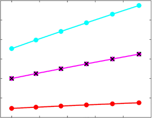
Figure 4. (a) Decomposition of the skin-friction coefficient $C_f$ into the terms in (3.23): $\mathcal {E}$ (red), $\mathcal {P}$ (blue), $\mathcal {C}$ (green) and $\mathcal {S}$ (orange). The magenta circles indicate the sum of all four components on the right-hand side of (3.23). The black crosses indicate $C_f$ obtained directly from the wall-shear stress data of Sillero et al. (Reference Sillero, Jiménez and Moser2013). (b) Integral lengths in (3.36): energy thickness $\mathbb {E}$ (cyan), inertia thickness $\mathbb {I}$ (red) and momentum thickness $\theta$ (black crosses). The magenta circles indicate $(\mathbb {E}+\mathbb {I})/2$. The $x$-axis is scaled by $x_1$, the coordinate of the first point. The momentum thickness $\theta$ at the six points is $4000, 4500, 5000, 5500, 6000, 6500$. The data in this figure are obtained by post-processing the results of the direct numerical simulations of Sillero et al. (Reference Sillero, Jiménez and Moser2013).

Similarly to the study of Renard & Deck (Reference Renard and Deck2016), (3.37) can be interpreted in the absolute frame of reference, i.e. where the wall is in motion. Equation (3.37) thus describes how the energy given by the wall motion to the fluid, measured by twice the change of $\theta$ with the streamwise direction, is divided into the change of $\mathbb {E}$, representing the losses of mean kinetic energy due to the mean-flow viscous dissipation into heat and to the production of turbulence, and the change of $\mathbb {I}$, representing the change in convective transport of the mean kinetic energy due to the mean velocity. The change of $\mathbb {I}$ can in turn be expressed as the sum of the changes of the thicknesses $\mathbb {C}$ and $\mathbb {S}$, which represent the change in transport due to the wall-normal mean velocity and the streamwise mean velocity, respectively. Referring to (3.7), we can now utilize the streamwise integral of (3.37) to investigate what percentage of the different terms in the RD decomposition contributes to the total drag by taking differences in the corresponding integral thicknesses.

It is noted, however, that the RD decomposition (3.22) and identities emerging from it, such as (3.37), do not distinguish the laminar and the turbulent contributions to the skin-friction coefficient for any flow, while the FIK identity achieves this task for confined flows and the identity discovered by Elnahhas & Johnson (Reference Elnahhas and Johnson2022) does so for free-stream boundary layers. As demonstrated by Renard & Deck (Reference Renard and Deck2016), the difference in the skin-friction coefficient between a laminar and a turbulent boundary layer at the same Reynolds number based on $\varDelta$ (for which $\mathcal {E}$ is identical) is dominated by $\mathcal {P}$.