2.1 Problem formulation

The basilisk solver is used to simulate the temporal and spatial evolution of a transversely forced planar liquid jet in a still ambient gas. The computational domain is square with an edge length $L=200D$, the inlet has a width $D=2\times 10^{-3}$ m and is located in the centre of the left boundary. The computational domain is significantly larger than the relevant area for this study. For the remaining sections of this work, only the area $-5<y/D<5$, $0<x/D<40$ will be considered and referred to as domain. The domain is initialised with $u_{i}=0$, $C=0$. We use Dirichlet boundary conditions at the inlet and impose a sinusoidal oscillation in the transverse velocity component. The inlet conditions at $\unicode[STIX]{x1D6FA}_{1}$ in the centre of the left domain edge reads

(2.4a)$$\begin{eqnarray}\displaystyle & \displaystyle u|_{\unicode[STIX]{x1D6FA}_{1}}=U, & \displaystyle\end{eqnarray}$$

(2.4b)$$\begin{eqnarray}\displaystyle & \displaystyle v|_{\unicode[STIX]{x1D6FA}_{1}}=U\times A\sin (2\unicode[STIX]{x03C0}f^{\ast }t), & \displaystyle\end{eqnarray}$$

(2.4c)$$\begin{eqnarray}\displaystyle & \displaystyle \left.\frac{\unicode[STIX]{x2202}p}{\unicode[STIX]{x2202}x}\right|_{\unicode[STIX]{x1D6FA}_{1}}=0, & \displaystyle\end{eqnarray}$$

(2.4d)$$\begin{eqnarray}\displaystyle & \displaystyle C|_{\unicode[STIX]{x1D6FA}_{1}}=1, & \displaystyle\end{eqnarray}$$

$U=4~\text{m}~\text{s}^{-1}$

$f^{\ast }=200$

$A=0.01,0.05$

$\unicode[STIX]{x1D6FA}_{2}$

$\unicode[STIX]{x1D6FA}_{3}$

$\unicode[STIX]{x1D6FA}_{4}$

(2.5a)$$\begin{eqnarray}\displaystyle & \displaystyle \frac{\unicode[STIX]{x2202}u_{i}}{\unicode[STIX]{x2202}x}|_{\unicode[STIX]{x1D6FA}_{4}}=0, & \displaystyle\end{eqnarray}$$

(2.5b)$$\begin{eqnarray}\displaystyle & \displaystyle p|_{\unicode[STIX]{x1D6FA}_{4}}=0, & \displaystyle\end{eqnarray}$$

(2.5c)$$\begin{eqnarray}\displaystyle & \displaystyle \frac{\unicode[STIX]{x2202}C}{\unicode[STIX]{x2202}x}|_{\unicode[STIX]{x1D6FA}_{4}}=0, & \displaystyle\end{eqnarray}$$

$x>L/4$

Figure 1. Schematic illustration of the computational domain and the adaptive grid (a) and grid sensitivity assessment using the streamwise development of the time-averaged shear layer momentum thickness $\unicode[STIX]{x1D6FF}$ for $A=0.05$ (b).

The fluid properties of the respective phases, corresponding to water and air, and the corresponding dimensionless quantities based on $U$, $D$ and the forcing frequency $f^{\ast }$ are given in tables 1, 2. The flow parameters and the domain extend are chosen such that the complete destabilisation cycle of the velocity field, including growth, saturation and onset of decay of the forced instability wave is captured within the area of interest. Further, the choice of flow parameters ensures that the jet remains intact throughout the domain such that no breakup of liquid structures occurs.

Table 1. Fluid properties of the liquid and gas phase.

Table 2. Dimensionless numbers, based on $U$, $D$ and the forcing frequency $f^{\ast }$.

A dynamic quadtree-structured grid is chosen as spatial domain discretisation. To check whether a cell needs refinement, its level is reduced by one and increased again. This corresponds to down- and up-sampling of the stored scalar fields. The original field $\unicode[STIX]{x1D713}$ is compared to the up-sampled field $\unicode[STIX]{x1D713}^{\ast }$ to estimate the error $\unicode[STIX]{x1D716}=\Vert \unicode[STIX]{x1D713}-\unicode[STIX]{x1D713}^{\ast }\Vert$. The cell is refined if $\unicode[STIX]{x1D716}>\unicode[STIX]{x1D703}$ and coarsened if $\unicode[STIX]{x1D716}<2/3\unicode[STIX]{x1D703}$ where $\unicode[STIX]{x1D703}$ is the error threshold of the specific scalar field. A more detailed description is given by van Hooft et al. (Reference van Hooft, Popinet, van Heerwaarden, van der Linden, de Roode and van de Wiel2018).

For the present work, we set $\unicode[STIX]{x1D703}=5\times 10^{-3}$ for both velocity components and the volume fraction. The maximum resolution is limited to $15$ levels of refinement, corresponding to a minimum non-dimensional cell edge length of $\unicode[STIX]{x0394}x/D\approx 0.0157$. To evaluate the adequacy of the chosen adaptation criteria and mesh resolution, the time-averaged shear layer momentum thickness, defined as

(2.6)$$\begin{eqnarray}\unicode[STIX]{x1D6FF}(x)=\int _{0}^{\infty }\frac{\overline{u}}{U}\left(1-\frac{\overline{u}}{U}\right)\,\text{d}y,\end{eqnarray}$$

where $\overline{u}$ denotes the time-averaged streamwise velocity, is shown for 13 to 15 levels of refinement in figure 1(b). No visible improvement is seen between the latter two levels, hence the chosen parameters should be sufficient.

Simulations are run for $TU/D=409.6$ non-dimensional time units, corresponding to $40.96$ oscillation cycles. Time stepping is adaptive based, on a Courant condition

(2.7)$$\begin{eqnarray}\unicode[STIX]{x0394}t\leqslant 0.5\min \left\{\frac{\unicode[STIX]{x0394}x}{u},\sqrt{\frac{\unicode[STIX]{x1D70C}_{l}\unicode[STIX]{x0394}x^{3}}{\unicode[STIX]{x03C0}\unicode[STIX]{x1D70E}}}\right\}.\end{eqnarray}$$

2.2 General jet evolution

The liquid jet, injected on the left side of the domain, evolves in the streamwise direction and remains intact throughout the area of interest. The harmonic transverse forcing at the inlet introduces an initially monochromatic wave that grows in space while being convected downstream. The disturbance amplitude is clearly visible in the fluid interface, shown in figure 2, for $A=0.01$ and $A=0.05$. For further illustration, the envelope of the interfacial instability wave is shown for both forcing amplitudes by plotting an iso-line of the time-averaged volume fraction field $\overline{C}$.

For both amplitudes, the interface disturbance grows in the streamwise direction over the whole domain. For $x>15D$ the interfacial disturbance wave starts saturating and approaches its maximum amplitude. The point where the interfacial disturbance is saturated completely is outside the investigated domain ($x/D\approx 45$). For $A=0.05$, the influence of the harmonic forcing on the interface is much more prominent, resulting in significantly larger amplitude growth. Further, for $A=0.05$ an increasing deviation from the initial wave pattern is evident from figure 2 for $x/D>20$. This results in a characteristic agglomeration of liquid around the wave crests as well as a shift from a sinuous wave shape to a triangular shape.

Figure 2. Instantaneous view of the interface via the volume fraction field $C$ for (a) $A=0.01$, (b) $A=0.05$. The blue area corresponds to $C>0.5$, denoting the liquid phase while the white area, $C<0.5$, denotes the gas phase. In (c) the envelope of the interfacial instability wave is shown as an iso-line of $\overline{C}=0.01$.

The spatio-temporal evolution of the interfacial wave and secondary structures is illustrated by the diagram of $C(x,y=0,t)$ and the instantaneous vorticity field $\unicode[STIX]{x1D6FA}=\unicode[STIX]{x2202}v/\unicode[STIX]{x2202}x-\unicode[STIX]{x2202}u/\unicode[STIX]{x2202}y$ in figure 3. The contour lines of $C$ illustrate the amplitude growth and saturation of the interfacial wave, while $\unicode[STIX]{x1D6FA}$ visualises the interaction of the interface with the instability growth in the respective fluid phases. Initially, the interfacial amplitude is small and the vorticity of the liquid phase is virtually zero, which is marked as the white area in the diagram. Downstream of approximately $x/D=10$, the amplitude growth leads to sufficient deflection of the interface to intermittently expose the growing non-zero gas-phase vorticity. In the subsequent development, the saturation of the interfacial wave is seen in the diagram as the gaps approach a constant thickness. The development of secondary structures is indicated by increasingly complex vortical patterns which manifest in the appearance of clockwise and anti-clockwise rotating vortical patterns in each gap during their downstream evolution.

Figure 3. Spatio-temporal diagram of the non-dimensional centreline vorticity $\unicode[STIX]{x1D6FA}/(U/D)(x,y=0,t)$ (filled contour) and the centreline volume fraction $C(x,y=0,t)=0.5$ (black contour line) for $A=0.05$.

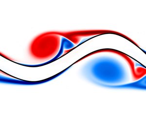
Figure 4. Instantaneous view of the non-dimensional vorticity field $\unicode[STIX]{x1D6FA}/(U/D)$ for (a) $A=0.01$, (b) $A=0.05$. The interface $C=0.5$ is shown as the black contour line.

For further clarification of the evolving vortical structures, the instantaneous vorticity field for both forcing amplitudes is shown in figure 4. For $A=0.01$, a single vorticity sheet evolves along each side of the interface and remains intact throughout its downstream development, indicating linear disturbance growth. Contrastingly, for $A=0.05$, the vorticity sheet in the initial shear layer is disturbed by the growing oscillation of the interface, which promotes agglomeration into discrete vortical structures from around $x/D\approx 15$. These structures develop along the interfacial wave crests when the curvature of the deflected interface becomes sufficiently large such that the vorticity sheet detaches from the interfacial curve. The formed structures travel in the wave troughs of the excited jet. While initially a single vortical structure is present, additional, secondary structures form during the downstream evolution of the jet.

Similar flow features are observable in the flow visualisation conducted by Tammisola et al. (Reference Tammisola, Sasaki, Lundell, Matsubara and Söderberg2011). In their experimental work a planar liquid sheet is sinusoidally forced with loudspeakers. Although their focus lies on frequency variation and the influence of gas co-flow, the sheet’s response to the forcing produces comparable results to this study. In particular, for higher amplitudes, the shift from a sinusoidal to a triangular wave pattern is clearly seen. The increased interface corrugations further suggest a pronounced influence of gas-phase vorticity on the jet.

A somewhat extreme illustration of the effects of large forcing amplitudes on a liquid jet is given in Schmidt et al. (Reference Schmidt, Krüger, Göckeler and Paschereit2018) where a liquid jet, emitted by an industrial-type fluidic oscillator, is studied numerically and experimentally. The primary instability mechanism studied in the present case is likely to play no role at that scale, as turbulence and early onset of breakup are too pronounced for instability growth to manifest. However, it is observable that the oscillation at large amplitudes, induces significant instabilities along the liquid jet surface. These in turn, have been found to drastically facilitate jet destabilisation, leading to reduced breakup length and smaller diameters in the produced droplet spectrum.

3.1 Perturbation and mean flow equations

The derivation of the perturbation equations is based on the Navier–Stokes equations for an incompressible Newtonian fluid. In contrast to § 2, they are formulated separately for each phase as

(3.1a)$$\begin{eqnarray}\displaystyle & \displaystyle \frac{\unicode[STIX]{x2202}u_{i,l,g}}{\unicode[STIX]{x2202}x_{i}}=0, & \displaystyle\end{eqnarray}$$

(3.1b)$$\begin{eqnarray}\displaystyle & \displaystyle \frac{\unicode[STIX]{x2202}u_{i,l,g}}{\unicode[STIX]{x2202}t}+u_{j,l,g}\frac{\unicode[STIX]{x2202}u_{i,l,g}}{\unicode[STIX]{x2202}x_{j}}=-\frac{\unicode[STIX]{x2202}p_{l,g}}{\unicode[STIX]{x2202}x_{i}}+\frac{1}{Re_{l,g}}\frac{\unicode[STIX]{x2202}^{2}u_{i,l,g}}{\unicode[STIX]{x2202}x_{j}^{2}}, & \displaystyle\end{eqnarray}$$

$l,g$

(3.2a,b)$$\begin{eqnarray}u_{i}(x_{i},t)=u_{b,i}(y)+\unicode[STIX]{x1D716}u_{i}^{\prime }(x_{i},t)\quad \text{and}\quad p(x_{i},t)=p_{b,i}(y)+\unicode[STIX]{x1D716}p^{\prime }(x_{i},t),\end{eqnarray}$$

where $\unicode[STIX]{x1D716}\ll 1$ is a small amplitude. The time-independent base flow is denoted by the subscript $b$. Since a local analysis is performed, the base flow is assumed to be parallel and of the form $u_{b,i}(y)=(u_{b}(y),0)^{\text{T}}$. The parameter $\unicode[STIX]{x1D716}$ will be dropped for the remainder of this work. The decomposition, equation (3.2), is substituted in (3.1). Since the base flow satisfies (3.1), all base flow terms vanish. By ignoring the nonlinear term $u_{j}^{\prime }(\unicode[STIX]{x2202}u_{i}^{\prime }/\unicode[STIX]{x2202}x_{j})$ the linearised form of the perturbation equations yields

(3.3a)$$\begin{eqnarray}\displaystyle & \displaystyle \frac{\unicode[STIX]{x2202}u_{i}^{\prime }}{\unicode[STIX]{x2202}x_{i}}=0, & \displaystyle\end{eqnarray}$$

(3.3b)$$\begin{eqnarray}\displaystyle & \displaystyle \frac{\unicode[STIX]{x2202}u_{i}^{\prime }}{\unicode[STIX]{x2202}t}+u_{b,j}\frac{\unicode[STIX]{x2202}u_{i}^{\prime }}{\unicode[STIX]{x2202}x_{j}}+u_{j}^{\prime }\frac{\unicode[STIX]{x2202}u_{b,i}}{\unicode[STIX]{x2202}x_{j}}=-\frac{\unicode[STIX]{x2202}p^{\prime }}{\unicode[STIX]{x2202}x_{i}}+\frac{1}{\mathit{Re}}\frac{\unicode[STIX]{x2202}^{2}u_{i}^{\prime }}{\unicode[STIX]{x2202}x_{j}^{2}}. & \displaystyle\end{eqnarray}$$

The equations describe the response of the underlying steady base flow to infinitesimal disturbances. However, basing the analysis on the base flow ignores any influence of dynamic fluctuations on the time-averaged mean flow such as the nonlinear saturation of the oscillatory flow (Noack et al. Reference Noack, Afanasiev, Morzyński, Tadmor and Thiele2003). Additionally, in case of an externally forced flow, a steady solution might not even exist. Therefore, since we are interested in the stability of the time-averaged flow, obtained from the oscillatory flow, once it has reached its limit cycle, it is appropriate to choose the triple decomposition of the flow field (Reynolds & Hussain Reference Reynolds and Hussain1972),

(3.4a,b)$$\begin{eqnarray}u_{i}(x_{i},t)=\overline{u}_{i}(y)+\tilde{u} _{i}(x_{i},t)+u_{i}^{\prime \prime }(x_{i},t)\quad \text{and}\quad p(x_{i},t)=\overline{p}(y)+\tilde{p}(x_{i},t)+p^{\prime \prime }(x_{i},t),\end{eqnarray}$$

where $\overline{u}_{i}$ and $\overline{p}$ are the time-averaged velocity and pressure field respectively, $\tilde{u} _{i}$, $\tilde{p}$ the periodic parts and $u_{i}^{\prime \prime }$, $p^{\prime \prime }$ the fluctuating parts. Upon substitution of the ansatz into (3.1), phase averaging and time averaging, the time-averaged Navier–Stokes equations are given as

(3.5a)$$\begin{eqnarray}\displaystyle & \displaystyle \frac{\unicode[STIX]{x2202}\overline{u}_{i}}{\unicode[STIX]{x2202}x_{i}}=0, & \displaystyle\end{eqnarray}$$

(3.5b)$$\begin{eqnarray}\displaystyle & \displaystyle \overline{u}_{j}\frac{\unicode[STIX]{x2202}\overline{u}_{i}}{\unicode[STIX]{x2202}x_{j}}=-\frac{\unicode[STIX]{x2202}\overline{p}}{\unicode[STIX]{x2202}x_{i}}+\frac{1}{\mathit{Re}}\frac{\unicode[STIX]{x2202}^{2}\overline{u}_{i}}{\unicode[STIX]{x2202}x_{j}^{2}}+{\mathcal{F}}_{i}, & \displaystyle\end{eqnarray}$$

(3.6)$$\begin{eqnarray}{\mathcal{F}}_{i}=-\frac{\unicode[STIX]{x2202}}{\unicode[STIX]{x2202}x_{j}}(\overline{\tilde{u} _{i}\tilde{u} _{j}})-\frac{\unicode[STIX]{x2202}}{\unicode[STIX]{x2202}x_{j}}(\overline{u_{i}^{\prime \prime }u_{j}^{\prime \prime }})\end{eqnarray}$$

is interpreted as nonlinear modification of the mean field by Reynolds stresses of the periodic and fluctuating field. This also implies that the mean flow is not a solution of the steady Navier–Stokes equation, as noted by Barkley (Reference Barkley2006).

The ansatz (3.4) is inserted in (3.1), phase averaging is performed and (3.5) is subtracted, to yield the dynamic equation of the fundamental wave

(3.7a)$$\begin{eqnarray}\displaystyle & \displaystyle \frac{\unicode[STIX]{x2202}\tilde{u} _{i}}{\unicode[STIX]{x2202}x_{i}}=0, & \displaystyle\end{eqnarray}$$

(3.7b)$$\begin{eqnarray}\displaystyle & \displaystyle \frac{\unicode[STIX]{x2202}\tilde{u} _{i}}{\unicode[STIX]{x2202}t}+\overline{u}_{j}\frac{\unicode[STIX]{x2202}\tilde{u} _{i}}{\unicode[STIX]{x2202}x_{j}}+\tilde{u} _{j}\frac{\unicode[STIX]{x2202}\overline{u}_{i}}{\unicode[STIX]{x2202}x_{j}}=-\frac{\unicode[STIX]{x2202}\tilde{p}}{\unicode[STIX]{x2202}x_{i}}+\frac{1}{\mathit{Re}}\frac{\unicode[STIX]{x2202}^{2}\tilde{u} _{i}}{\unicode[STIX]{x2202}x_{j}^{2}}+{\mathcal{F}}_{i}^{\ast }, & \displaystyle\end{eqnarray}$$

(3.8)$$\begin{eqnarray}{\mathcal{F}}_{i}^{\ast }=-\frac{\unicode[STIX]{x2202}}{\unicode[STIX]{x2202}x_{j}}(\tilde{u} _{i}\tilde{u} _{j})-\frac{\unicode[STIX]{x2202}}{\unicode[STIX]{x2202}x_{j}}(\widetilde{{u^{\prime \prime }}_{i}{u^{\prime \prime }}_{j}}).\end{eqnarray}$$

For the mean flow analysis, we assume that the influence of the quadratic harmonic interactions is small, although the harmonic waves themselves might not necessarily be small. Further, we assume the fluctuating velocity is small compared to the harmonic velocity (which is demonstrated in § 5). We therefore ignore ${\mathcal{F}}_{i}^{\ast }$ and conduct an a posteriori analysis of the nonlinear terms in § 5 to check the validity of this assumption.

3.2 Solution method and validation

The coherent perturbations are decomposed into Fourier modes

(3.9a,b)$$\begin{eqnarray}\tilde{u} _{i}(x_{i},t)=\hat{u} _{i}(y)\text{e}^{\unicode[STIX]{x1D704}(\unicode[STIX]{x1D6FC}x-\unicode[STIX]{x1D714}t)}\quad \text{and}\quad \tilde{p}(x_{i},t)=\hat{p}(y)\text{e}^{\unicode[STIX]{x1D704}(\unicode[STIX]{x1D6FC}x-\unicode[STIX]{x1D714}t)},\end{eqnarray}$$

where $\unicode[STIX]{x1D704}$ denotes the imaginary unit, $\unicode[STIX]{x1D6FC}$ the streamwise wavenumber of the perturbation and $\unicode[STIX]{x1D714}$ the streamwise frequency, both of which are generally complex; $\hat{u} _{i}$ and $\hat{p}$ are the complex eigenfunctions of respective perturbations in velocity and pressure. We are interested in the spatial growth and decay of disturbances. Hence, a spatial stability analysis is pursued where $\unicode[STIX]{x1D714}$ is a known, real valued frequency and $\unicode[STIX]{x1D6FC}$ is complex valued and unknown. The ansatz (3.9) is introduced in (3.7) to obtain the Fourier-transformed perturbation equations.

Note, that the assumption of a parallel mean flow in the present case is worth questioning. In case of a laminar unforced jet, the liquid phase might retain an approximately constant diameter and an unaltered velocity profile between two respective downstream positions. This is the case if the jet exhibits a block-like velocity profile, as in e.g. Tammisola et al. (Reference Tammisola, Sasaki, Lundell, Matsubara and Söderberg2011). However, for a parabolic inflow profile (Söderberg Reference Söderberg2003), the liquid interfaces notably contracts until it reaches a relaxed state. Additionally, the shear layer spreading within the gaseous phase invalidates the strict assumption of a parallel flow.

In case of a forced jet as in the present case, the downstream spreading of the mean flow certainly violates the parallel flow assumption for both phases. Nevertheless, local analysis has shown remarkable robustness in predicting stability properties for a variety of non-parallel flows (see e.g. Cohen & Wygnanski Reference Cohen and Wygnanski1987; Pier Reference Pier2002; Oberleithner, Paschereit & Wygnanski Reference Oberleithner, Paschereit and Wygnanski2014a; Terhaar, Oberleithner & Paschereit Reference Terhaar, Oberleithner and Paschereit2015; Emerson, Lieuwen & Juniper Reference Emerson, Lieuwen and Juniper2016). Alternatively, axial spreading can be accounted for by using a correction scheme for weakly non-parallel flows by introducing a slowly varying axial scale (Crighton & Gaster Reference Crighton and Gaster1976; Oberleithner et al. Reference Oberleithner, Rukes and Soria2014b) or within the framework of parabolised stability equations (Herbert Reference Herbert1997; Cheung & Zaki Reference Cheung and Zaki2010). Yet, another approach is to compute the optimal response to a forcing from the resolvent norm around the mean flow, taking into account the non-normality of the linearised operator (Beneddine et al. Reference Beneddine, Sipp, Arnault, Dandois and Lesshafft2016). However, for the present work, the focus lies on the applicability of a simple linear model to capture the overall phenomena of the underlying nonlinear flow. A detailed representation is already available through the nonlinear simulation results. Therefore, we stick to the parallel flow assumption.

As noted above, for the analysis of immiscible interfacial flows, the perturbation equations are formulated separately for each phase (see e.g. Söderberg Reference Söderberg2003; Gordillo & Pérez-Saborid Reference Gordillo and Pérez-Saborid2005). By imposing symmetry conditions along the jet centreline, it is sufficient to only consider the top half of the jet. At the interface position, coupling conditions are formulated to satisfy (3.7) across the interface. Formally the interface position is of the form $y=h(x,t)$ and is assumed to be decomposed and perturbed similarly to (3.4) (where the fluctuations are neglected) and (3.9) so that

(3.10a,b)$$\begin{eqnarray}h(x,t)=\overline{h}(x)+\tilde{h}(x,t)\quad \text{and}\quad \tilde{h}(x,t)={\hat{h}}(x)\text{e}^{\unicode[STIX]{x1D704}(\unicode[STIX]{x1D6FC}x-\unicode[STIX]{x1D714}t)}.\end{eqnarray}$$

For an unforced jet, the mean interface position is assumed to be approximately equal to the unperturbed interface position of the steady base flow, which is taken to be constant in $x$. Hence, $\overline{h}$ is constant. In the time-averaged flow of the forced state it is not. Following the triple decomposition, $\overline{h}$ should be obtained by time averaging the instantaneous interface positions at each $x$. However, this approach yields unsatisfactory results as seen in § 4. Therefore, an alternative modelling approach is given in § 3.3 which does not follow the triple decomposition.

For the derivation of the coupling conditions, a constant $\overline{h}$ is assumed. Formally, these conditions are valid at the perturbed interface $h(x,t)$. However, by means of a Taylor expansion of $h(x,t)$ around $y=\overline{h}$ and by neglecting terms of second order or higher, a linear approximation at the unperturbed interface is obtained. In the following, the approximated conditions at the unperturbed interface are presented. For satisfying the continuity of the velocity across the interface, it holds that

(3.11a)$$\begin{eqnarray}\displaystyle & \displaystyle \left.\unicode[STIX]{x27E6}\tilde{u} +\overline{u}+\tilde{h}\frac{\text{d}\overline{u}}{\text{d}y}\right.\unicode[STIX]{x27E7}_{y=\overline{h},l}-\left.\unicode[STIX]{x27E6}\tilde{u} +\overline{u}+\tilde{h}\frac{\text{d}\overline{u}}{\text{d}y}\right.\unicode[STIX]{x27E7}_{y=\overline{h},g}=0, & \displaystyle\end{eqnarray}$$

(3.11b)$$\begin{eqnarray}\displaystyle & \displaystyle \unicode[STIX]{x27E6}\tilde{v}\unicode[STIX]{x27E7}_{y=\overline{h},g}-\unicode[STIX]{x27E6}\tilde{v}\unicode[STIX]{x27E7}_{y=\overline{h},l}=0, & \displaystyle\end{eqnarray}$$

$\unicode[STIX]{x27E6}\cdot \unicode[STIX]{x27E7}_{y=\overline{h},l,g}$

(3.12)$$\begin{eqnarray}\left.\unicode[STIX]{x27E6}\frac{\unicode[STIX]{x2202}\tilde{v}}{\unicode[STIX]{x2202}x}+\frac{\unicode[STIX]{x2202}\tilde{u} }{\unicode[STIX]{x2202}y}+\tilde{h}\frac{\text{d}^{2}\overline{u}}{\text{d}y^{2}}\right.\unicode[STIX]{x27E7}_{y=\overline{h},l}-m\left.\unicode[STIX]{x27E6}\frac{\unicode[STIX]{x2202}\tilde{v}}{\unicode[STIX]{x2202}x}+\frac{\unicode[STIX]{x2202}\tilde{u} }{\unicode[STIX]{x2202}y}+\tilde{h}\frac{\text{d}^{2}\overline{u}}{\text{d}y^{2}}\right.\unicode[STIX]{x27E7}_{y=\overline{h},g}=0,\end{eqnarray}$$

and the continuity of normal stress yields

(3.13)$$\begin{eqnarray}\left.\unicode[STIX]{x27E6}\tilde{p}-\frac{2}{Re_{l}}\frac{\unicode[STIX]{x2202}\tilde{v}}{\unicode[STIX]{x2202}y}\right.\unicode[STIX]{x27E7}_{y=\overline{h},l}-\left.\unicode[STIX]{x27E6}r\tilde{p}-\frac{2m}{Re_{l}}\frac{\unicode[STIX]{x2202}\tilde{v}}{\unicode[STIX]{x2202}y}\right.\unicode[STIX]{x27E7}_{y=\overline{h},g}+\frac{1}{We}\frac{\unicode[STIX]{x2202}^{2}\tilde{h}}{\unicode[STIX]{x2202}x^{2}}=0,\end{eqnarray}$$

where $m=\unicode[STIX]{x1D707}_{g}/\unicode[STIX]{x1D707}_{l}$ is the ratio of the dynamic viscosities of the two fluids and $r=\unicode[STIX]{x1D70C}_{g}/\unicode[STIX]{x1D70C}_{l}$ is the density ratio. A detailed derivation of the stress conditions is given in appendix A. The kinematic condition for the interface is

(3.14)$$\begin{eqnarray}\left.\unicode[STIX]{x27E6}\frac{\unicode[STIX]{x2202}\tilde{h}}{\unicode[STIX]{x2202}t}+\overline{u}\frac{\unicode[STIX]{x2202}\tilde{h}}{\unicode[STIX]{x2202}x}=\tilde{v}\right.\unicode[STIX]{x27E7}_{y=\overline{h},l,g}.\end{eqnarray}$$

Note that it is possible to formulate the kinematic condition for the gas-phase velocity at the interface as well as for the liquid-phase velocity. The coupling conditions are complemented by boundary conditions to close the system.

Only asymmetric waves are considered in the stability analysis, since in the nonlinear simulation, the jet is forced sinusoidally in the $v$-component of the velocity to excite asymmetric modes. From the analysis of the simulation it is evident that the dominant mode at the forcing frequency remains asymmetric throughout the downstream development of the jet and the aim of the work is to investigate the potential of the mean flow stability model to predict the growth and saturation of this forced wave. Therefore, a symmetry condition

(3.15)$$\begin{eqnarray}\left.\unicode[STIX]{x27E6}\tilde{u} =0,\frac{\unicode[STIX]{x2202}\tilde{v}}{\unicode[STIX]{x2202}y}=0,\tilde{p}=0\right.\unicode[STIX]{x27E7}_{y=0,l}\quad \text{for asymmetric modes}\end{eqnarray}$$

is imposed, as well as a no-slip condition

(3.16)$$\begin{eqnarray}\left.\unicode[STIX]{x27E6}\frac{\unicode[STIX]{x2202}\tilde{u} }{\unicode[STIX]{x2202}y}=0,\tilde{v}=0,\frac{\unicode[STIX]{x2202}\tilde{p}}{\unicode[STIX]{x2202}y}=0\right.\unicode[STIX]{x27E7}_{y\rightarrow \infty ,g}.\end{eqnarray}$$

The closed system (equations (3.7), (3.11)–(3.16)) with the ansatz (3.9), (3.10) is solved using a Chebyshev spectral collocation method. The grid of the liquid phase extends over $0<y\leqslant \overline{h}(x)$ where $\overline{h}(x=0)=0.5$. The grid of the gas phase extends from $\overline{h}(x)<y\leqslant 4D$. Each grid is discretised using $N=110$ collocation points, resulting in $2\times N\times 3=1980$ degrees of freedom. Convergence is demonstrated in appendix B. The resulting quadratic eigenvalue problem is of the form

(3.17)$$\begin{eqnarray}(\unicode[STIX]{x1D6FC}^{2}\unicode[STIX]{x1D63C}_{2}+\unicode[STIX]{x1D6FC}\unicode[STIX]{x1D63C}_{1}+\unicode[STIX]{x1D63D})\boldsymbol{q}=\mathbf{0}.\end{eqnarray}$$

The matrices $\unicode[STIX]{x1D63C}_{2}$, $\unicode[STIX]{x1D63C}_{1}$ and $\unicode[STIX]{x1D63D}$ contain the mean flow profiles $\overline{u}_{l,g}$, and $\boldsymbol{q}=(\hat{u} _{l},\hat{v}_{l},\hat{p}_{l},\hat{u} _{g},\hat{v}_{g},\hat{p}_{g},{\hat{h}})^{\text{T}}$. Using the companion linearisation, equation (3.17) is reduced to a linear problem

(3.18)$$\begin{eqnarray}\left[\left(\begin{array}{@{}cc@{}}\unicode[STIX]{x1D63D} & \mathbf{0}\\ \mathbf{0} & \unicode[STIX]{x1D644}\end{array}\right)+\unicode[STIX]{x1D6FC}\left(\begin{array}{@{}cc@{}}\unicode[STIX]{x1D63C}_{1} & \unicode[STIX]{x1D63C}_{2}\\ -\unicode[STIX]{x1D644} & \mathbf{0}\end{array}\right)\right]\left(\begin{array}{@{}c@{}}\boldsymbol{q}\\ \unicode[STIX]{x1D6FC}\boldsymbol{q}\end{array}\right)=\mathbf{0},\end{eqnarray}$$

where $\unicode[STIX]{x1D644}$ is the identity matrix. The linear system, equation (3.18), is consecutively solved at each streamwise position using the $QZ$ algorithm in matlab’s eig function, which simultaneously delivers all eigenvalues, to obtain the spatial evolution of $\unicode[STIX]{x1D6FC}$ and the corresponding eigenfunctions. The additional eigenvalues and eigenvectors, introduced by the companion linearisation, are discarded. To validate the code, the temporal stability results of the two-layer Poiseuille flow by Dongarra, Straughan & Walker (Reference Dongarra, Straughan and Walker1996) are reproduced. The resulting unstable eigenvalues are listed in table 3 and the flow conditions are restated in appendix C. As their results exclude the influence of surface tension, the results of Tammisola et al. (Reference Tammisola, Sasaki, Lundell, Matsubara and Söderberg2011) (figure 16a) in their work) are qualitatively reproduced as well.

Table 3. Validation of two-layer Poiseuille flow using temporal analysis ($\unicode[STIX]{x1D6FC}=1$). The corresponding unstable eigenvalues $c\equiv \unicode[STIX]{x1D714}/\unicode[STIX]{x1D6FC}$ are displayed.

3.3 Mean flow configuration and parameterisation

The $u$-component of the mean flow velocity field is obtained by averaging $2^{11}$ consecutive snapshots of the fully developed flow of the nonlinear simulation in § 2 at time increments $\unicode[STIX]{x0394}tU/D=0.15$ and within an area $-5<y/D<5$, $0<x/D<40$. These are mapped on an equidistant Cartesian grid with a resolution of $800\times 200~\text{px}$ where $1~\text{px}=1\times 10^{-4}~\text{m}$. The mean flow field should be symmetric with respect to the jet centreline. Therefore, remaining minor asymmetries in the time-averaged flow are eliminated by taking the symmetric part

(3.19)$$\begin{eqnarray}\overline{u}_{sym}={\textstyle \frac{1}{2}}(\overline{u}(y)+\overline{u}(-y)).\end{eqnarray}$$

The symmetric, time-averaged mean flow is shown in figure 6.

In Gordillo & Pérez-Saborid (Reference Gordillo and Pérez-Saborid2005) and Tammisola et al. (Reference Tammisola, Sasaki, Lundell, Matsubara and Söderberg2011) analytic base flows were used and a constant velocity profile of the liquid phase was assumed. The gas boundary layer was approximated using an error-function profile. A comparison of the mean flow profiles with these analytic profiles is given in figure 5. It is seen that for the unforced flow, the error-function profile slightly over-estimates the developing shear layer, although differences are minor. More prominent deviations are observed along the interface, since the assumption of a constant liquid velocity does not hold for the nonlinear simulation. Further, the zero Dirichlet condition for the gas velocity causes a reversed flow in the gas phase close to the inlet, which possibly influences the development of the initial boundary layer and could have an effect on the growth rate of the instability wave. For the forced flow, the mean flow profile quickly deviates from the error-function profile, as the oscillation significantly thickens the mean flow shear layer, especially for $A=0.05$. In conclusion, the analytic profile might be a sufficient approximation for an unforced jet but not for a forced jet.

Figure 5. Comparison of the mean flow profiles and an error-function profile (as in Tammisola et al. (Reference Tammisola, Sasaki, Lundell, Matsubara and Söderberg2011)) for the unforced flow (a), and forced flow with (b) $A=0.01$, (c) $A=0.05$. Plot positions are $x/D=0.01,1,2,5,10,20$. For $A=0.05$, positions $x/D=10,20$ are omitted due to very large deviations from the error-function profile.

The necessity of modelling the position of the mean interface in the mean flow, noted in the previous section, is addressed here. Within the parallel flow framework, the interface between the liquid and gaseous phase is located at a fixed position $y=h_{b}$ which is determined by the solution of the underlying steady base flow. For instance, in Tammisola et al. (Reference Tammisola, Sasaki, Lundell, Matsubara and Söderberg2011) and Gordillo & Pérez-Saborid (Reference Gordillo and Pérez-Saborid2005) the interface position remained constant in downstream direction. In Söderberg (Reference Söderberg2003) a numerical base flow for the liquid phase was computed with varying interface positions in downstream direction.

For this study a simple model is constructed, that requires the mass of the liquid phase at $x/D=0$ to be conserved for all streamwise positions in the mean flow. The initial mass is determined by the initial interface position $\overline{h}(x=0)=0.5$. Then, the time-averaged density field $\overline{\unicode[STIX]{x1D70C}}$ is integrated at each $x$, from $0<y<\overline{h}(x)$. The upper integration bound $\overline{h}(x)$, defining the interface within the mean flow, is chosen such that

(3.20)$$\begin{eqnarray}\int _{0}^{0.5}\frac{\overline{\unicode[STIX]{x1D70C}}(x=0,y)}{\unicode[STIX]{x1D70C}_{l}D}\,\text{d}y=\int _{0}^{\overline{h}(x)}\frac{\overline{\unicode[STIX]{x1D70C}}(x,y)}{\unicode[STIX]{x1D70C}_{l}D}\,\text{d}y.\end{eqnarray}$$

An illustration of this procedure is shown in figure 7 along with the resulting interface curve within the mean flow. As is seen, the model moves the interface reasonably into the mean flow shear layer.

Figure 6. Mean flow profiles of the jet forced at $A=0.01$ (blue); $A=0.05$ (black). The spreading of the mean interface position, derived from figure 7, is shown as a dashed line.

Figure 7. Illustration of the mean interface spreading. The top row shows a contour plot of the mean volume fraction field $\overline{\unicode[STIX]{x1D70C}}/\unicode[STIX]{x1D70C}_{l}$ of the nonlinear simulation and the interpolated interface position for the linear stability model as black line, for (a) $A=0.01$; (b) $A=0.05$. The black dotted line represents the presumed, fixed interface position of the unforced flow. Red areas correspond to regions of small interface amplitudes while lighter shades indicate areas of increased amplitudes. The second row shows the cumulative integral of $\overline{\unicode[STIX]{x1D70C}}/\unicode[STIX]{x1D70C}_{l}D$ along $y$ for several streamwise positions, for (c) $A=0.01$; (d) $A=0.05$. The interface at $x=0$ (vertical line) determines the initial mass of the liquid. The interface is constructed such that the liquid mass is conserved (horizontal line).

When using a true stationary solution, the interface position can simply be defined by the volume fraction $C=0.5$, as in the VoF method. However, this assumption does not hold in the time-averaged flow (for the time-averaged volume fraction $\overline{C}\approx \overline{\unicode[STIX]{x1D70C}}/\unicode[STIX]{x1D70C}_{l}$) which is seen in figure 7: Using $\overline{C}=0.5$ the interface would move towards the centreline of the jet. A consistent approach to obtaining the interface position according to the triple decomposition would be to take the time-averaged position. However, for a transverse sinusoidal forcing, the growing interface disturbance should approximate a growing sine wave on each side of the plane jet/sheet. As the jet oscillates symmetrically around its (theoretical) centreline, the time-averaged position of the interface would be $\overline{h}(x)=\pm 0.5$ for all streamwise positions, which corresponds to the position of the unperturbed flow. Another approach to obtain the interface position in the mean flow that might seem plausible at first sight, is to derive the location with the highest probability of interface residence at each streamwise position, i.e. a probability density. However, for a sine wave this would yield an interface position at either of the extrema of the sine wave. This does not seem plausible, since it traverses the interface almost out of the mean flow shear layer. The effect of the interface correction is further assessed in the following sections.

3.4 General stability properties of the jet

For the stability analysis, three different cases will be of interest. The first case is based on the mean flow of the unforced jet. As within the current numerical framework, natural disturbances of the unforced jet remain very small (at least in the considered domain), it closely corresponds to an equilibrium or base flow solution, i.e. the interface remains at the initial, unperturbed position within the sampling accuracy ($\overline{h}(x)=0.5$), as has been carefully checked. We denote this case as the base flow model. The second case is based on the mean flow of the forced jet but ignores the interface displacement in the mean flow, such that $\overline{h}(x)=0.5$ (equivalent to a triple decomposition of the interface). This case is denoted as the fixed interface model. The third case is similar to the second one but includes the proposed interface correction model to account for the interface displacement. This case is denoted as the varying interface model.

To obtain a general overview on the stability properties of the present jet configuration, in figures 8(a) and 8(b) the streamwise distribution of spatial growth rates is derived for the base flow model for a broad range of frequencies. There are two unstable modes found which together render the jet convectively unstable for all applied frequencies within the displayed domain.

In detail, mode I is unstable for all shown frequencies and shows an increasing maximum growth rate as the frequency increases up to $fD/U=0.27$. Characteristic for this mode are the almost vertical contour lines within the initial region of the jet, that make the upstream stability behaviour of the jet virtually similar for a range of applied frequencies of approximately $0.1<fD/U<0.3$. The upstream appearance of the mode is qualitatively reminiscent of the sinuous mode of type I found in Söderberg (Reference Söderberg2003).

For frequencies $fD/U<0.27$ mode II is unstable as well in the upstream region of the jet. However, prolonged downstream influence of this mode is only observed for $fD/U<0.1$, where the point of neutral stability moves beyond $x/D=10$. Contrasting with mode I, the contour lines follow a more horizontal trend, especially in the lower frequencies. Additionally, the mode shows significantly smaller growth rates within the initial jet region, compared to mode I. The low-frequency region of this mode partially resembles the sinuous mode of type II found in Söderberg (Reference Söderberg2003). For better comparison the stability maps are re-plotted in appendix D, using similar scaling as in Söderberg (Reference Söderberg2003). However, in contrast to his findings, no third unstable physical eigenvalue is found for the present configuration.

There is however one additional marginally stable eigenvalue found which might correspond to the third mode found in Söderberg (Reference Söderberg2003), but since it is not unstable we shall not investigate it further in this work. Also mode II is either stable or exhibits weaker growth for the forcing frequencies applied in this work and thus will be excluded from further investigations as well.

The stability map of mode I is also derived for the fixed and varying interface model with $A=0.01$ at $\mathit{St}=0.1$ in figure 8(d). As can be seen, the mean flow for the fixed interface model significantly alters the stability map. Using the forced flow, the threshold for neutral stability moves into the domain for all frequencies and is located between $x/D=20$ and $x/D=30$ for $fD/U>0.05$. For lower frequencies the neutral point reaches approximately $x/D=10$. When the displacement of the mean interface position is taken into account (varying interface model), the neutral stability curve shifts even further upstream for most frequencies and renders all positions downstream $x/D=20$ stable. This indicates that the spreading of the mean interface has indeed an impact on the stability properties of the jet even at small forcing amplitudes and as shown below is even necessary to correctly recover the point of neutral stability of the excited instability wave. The maps derived for the fixed and varying interface model are obtained using the time-averaged flow at $St=0.1$. Therefore, the growth rates shown in figures 8(c) and 8(d) correspond to modes existing on this specific mean flow. For deriving maps where the displayed growth rates correspond to the most unstable eigenmode at the forcing frequency, a separate mean flow with a forcing at the respective frequency would have to be used for each eigenmode.

Figure 8. Stability map for the base flow model: mode I (a), mode II (b), fixed interface model (mode I) at $A=0.01$ (c), varying interface model (d). Shown is the spatial growth rate $-\unicode[STIX]{x1D6FC}_{\unicode[STIX]{x1D704}}D$ and the curve indicating neutral stability, i.e. $\unicode[STIX]{x1D6FC}_{\unicode[STIX]{x1D704}}D=0$, in red.

The origin of the unstable mode can be inspected by analysing its energy budget, as carried out by Boomkamp & Miesen (Reference Boomkamp and Miesen1996) and Otto (Reference Otto2012). Therefore, an energy balance over both fluid phases is derived as

(3.21)$$\begin{eqnarray}\text{MFL}_{l}+\text{MFL}_{g}=\text{REY}_{l}+\text{REY}_{g}+\text{TAN}+\text{NOR}+\text{DIS}_{l}+\text{DIS}_{g},\end{eqnarray}$$

where $\text{MFL}$ corresponds to the streamwise mean energy flux. The flux is balanced by a production term accounting for energy transfer from the mean flow to the perturbation through Reynolds stresses $\text{REY}$. The energy transfer to the velocity perturbations along the interface is accounted for by $\text{TAN}$ and $\text{NOR}$, representing the work of tangential and normal stress. The perturbation energy dissipation is given by $\text{DIS}$. It is always negative by definition while the sign of the other quantities might change depending of the flow configuration. Every quantity is normalised by the sum of all quantities. The complete expressions for the respective terms are given in appendix E. The contributions of the respective terms, calculated exemplarily at $x/D=10$, are given table 4.

For $A=0.01$ the energy budget is dominated by the contribution of tangential stresses, caused by the viscosity jump across the interface. Additionally, the energy transfer from the mean flow to the perturbed flow through Reynolds stresses within the liquid phase as well as the contribution of normal stresses from the pressure jump have some influence, although they are significantly weaker than the tangential stresses. Energy dissipation almost exclusively takes place in the liquid phase. Overall the gaseous phase has negligible contribution to the perturbation energy budget. For increased forcing the influence of $\text{TAN}$ and $\text{REY}_{g}$ decreases while for $\text{REY}_{l}$ and $\text{NOR}$ it increases.

The interface correction is seen to increase the influence of the $\text{REY}_{l}$ and lower the influence of $\text{TAN}$ which is to be expected since the correction shifts the interface position outwards into the mean flow shear layer where the mean flow gradient is larger than in proximity to the jet centreline and so are the Reynolds stresses.

When comparing the contributions at the respective amplitudes it is seen that the contribution of $\text{REY}_{g}$ decreases for increasing forcing amplitude which seems counter-intuitive. However, due to the increased mean flow spreading for larger forcing amplitudes, the transverse gradient of the mean flow velocity in the gas phase, as seen in figure 6, reduces which provides an explanation for the lower values of $\text{REY}_{g}$. In contrast, the gradient within the liquid part of the mean flow shows a slight increase which is in line with the increase of $\text{REY}_{l}$ for larger forcing amplitudes.

Table 4. Energy budget of mode I of the linear stability model at $x/D=10$.

4.1 Streamwise and cross-wise eigenfunctions

The eigenfunctions $\hat{u}$ and $\hat{v}$ of the linear stability analysis and the fundamental wave packet ($n=1$) of the DNS, derived from (4.1), are shown in figure 9. The region of linear growth is followed by the nonlinear saturation and decay of the amplitude.

For $A=0.01$ and the fixed interface model, an overall very good agreement is found for $\hat{v}$. Particularly in the gaseous part of the shear layer, there is an excellent correspondence of the eigenfunctions throughout the domain. Along the liquid jet centreline, amplitude prediction is very good as well up to approximately $x/D=20$. However, beyond that point there are some visible discrepancies around the interface where the steep gradient of the amplitude is not followed as rigorously by the linear model. For $x/D>30$ the agreement between simulation and linear stability model deteriorates further within the liquid part of the shear layer. The under-prediction for $x/D<5$ within the liquid phase is possibly attributed to the influence of the inlet wall in the simulation, which should approximately resemble the nozzle in the experiments of Orszag & Crow (Reference Orszag and Crow1970) and Oberleithner et al. (Reference Oberleithner, Rukes and Soria2014b). They argue that discrepancies in this area are likely caused by an interaction of the instability wave with the nozzle that is not covered by the linear model. For $\hat{u}$ similar agreement is found. The discrepancies along the interface are seen here as well and visualised as a slight lateral shift of the amplitude maximum.

For the varying interface model the eigenfunctions of linear stability analysis and their equivalents of the DNS become virtually indistinguishable throughout the domain (apart from the near-nozzle region that remains unaffected by the correction). This shows that accounting for the displacement interface in the spreading mean flow is indeed necessary to obtain a correct representation of the eigenfunctions. In conjunction with the findings in table 4, neglecting the interface spreading leads to a under-representation of Reynolds stresses in the mean flow stability model and an insufficient representation of the perturbation shear layer.

For $\hat{u}$ a similar trend is found. With the fixed interface model, increasing discrepancies along the interface are seen here as well for $x/D>15$ and manifest in the absence of a lateral shift of the amplitude maximum as well as the formation of an erroneous double spike in the amplitude. For the varying interface model, the outward spreading of the amplitude is followed by the linear model.

For $A=0.05$, the overall agreement is significantly less accurate. Nevertheless for $x/D<20$, the $\hat{v}$-component shows very good agreement despite the significant transverse spreading of the shear layer (varying interface model). With the fixed interface model this trend is not followed, resulting in visible deviations already at $x/D=7.5$. However, beyond $x/D=20$ both methods fail to correctly represent the wave packet amplitude of the nonlinear flow. The portray of $\hat{u}$ shows the same trend, though the qualitative differences are somewhat more pronounced.

Figure 9. Illustration of the fundamental wave packet ($n=1$), obtained from the DNS and comparison of the computed amplitude functions from the linear stability model and the DNS for (a) $A=0.01$, $\hat{u}$; (b) $A=0.01$, $\hat{v}$; (c) $A=0.05$, $\hat{u}$; (d) $A=0.05$, $\hat{v}$. Panels show, from top to bottom, the real part, imaginary part, the absolute value and corresponding amplitudes (for the fixed and varying interface model) normalised by their maximum value. Blue lines show the DNS while black lines show the LSA.

4.2 Growth rates and phase velocity

In the linear model, growth rates of the instability wave are readily given through the imaginary part of the eigenvalue $\unicode[STIX]{x1D6FC}_{\unicode[STIX]{x1D704}}$, introduced in (3.9). Deriving a correspondent measure for the amplitude growth from the DNS introduces an ambiguity to the analysis. For the present work, the most suitable measure was found to be based on the energy norm of the two-phase velocity field. The amplitude is computed as

(4.2)$$\begin{eqnarray}\tilde{A}_{n}(x;\hat{\unicode[STIX]{x1D70C}}_{n};\hat{u} _{n};\hat{v}_{n})=\frac{\sqrt{2}}{UD/2}\left(\int _{0}^{\infty }|\hat{\unicode[STIX]{x1D70C}}_{n}|[|\hat{u} _{n}|^{2}+|\hat{v}_{n}|^{2}]\,\text{d}y\right)^{1/2},\end{eqnarray}$$

where $\hat{\unicode[STIX]{x1D70C}}_{n},\hat{u} _{n},\hat{v}_{n}$ are obtained from (4.1). This corresponds to the amplitude of the velocity fluctuation of the respective harmonics, integrated across the shear layer of the jet (Delbende, Chomaz & Huerre Reference Delbende, Chomaz and Huerre1998; Oberleithner et al. Reference Oberleithner, Rukes and Soria2014b). Other plausible energy norms include a separate formulation for the velocity of the respective fluid phases or a formulation for the density field only. A separate measure of the velocity of each fluid phase did not reveal any significant differences in the evolution of the growth rates as compared to the chosen method. However, when using a formulation over the density field, a slower decay of the instability wave is observed (not shown). The streamwise growth rate then is defined as

(4.3)$$\begin{eqnarray}-\tilde{\unicode[STIX]{x1D6FC}}_{\unicode[STIX]{x1D704}}(x)=\frac{\text{d}(\ln \tilde{A}_{1})}{\text{d}x}.\end{eqnarray}$$

The predicted growth rates of both models are given in figure 10. For $A=0.01$, very good agreement is reached between the DNS and the linear stability model. For the fixed interface model, the growth rates in the initial region up to $x/D=5$ are very well recovered. Thereafter, the predicted growth rate decreases slower than in the DNS leading to a slightly delayed saturation and zero crossing of the growth rate of the linear model. Further downstream, the stable wave decays slightly slower than predicted by the DNS. Using the varying interface model, the initial growth rate is slightly over-predicted. However, for $10<x/D<30$ an excellent agreement is found and the neutral point is (if slightly under-predicted) recovered better than for the fixed interface model. In comparison, the growth rates obtained from the base flow model (appendix F) do not predict the neutral point to be within the considered domain at all. Therefore, the mean flow model generally seems to yield more accurate results than the base flow model.

For $A=0.05$ in figure 10(b), the agreement of the predicted growth rates is poor throughout the domain, which is to be expected from the substantial deviations of the eigenfunctions shown above. The fixed interface model predicts the instability wave to decay much faster than in the DNS, leading to a significant under-prediction of the neutral point. For the varying interface model, the growth rate prediction of the linear model is even worse and predicts an increasing destabilisation of the instability wave such that no saturation is predicted at all.

Figure 10. Comparison of the computed growth rates $-\unicode[STIX]{x1D6FC}_{\unicode[STIX]{x1D704}}D$ from the linear stability model and $-\tilde{\unicode[STIX]{x1D6FC}}_{\unicode[STIX]{x1D704}}D$ from the DNS for (a) $A=0.01$, (b) $A=0.05$. DNS denotes the nonlinear simulation, LSAv and LSAf the varying and fixed interface model.

To compare the real part of the eigenvalue, $\unicode[STIX]{x1D6FC}_{\unicode[STIX]{x1D70C}}$, to the wavelength of the forced instability, observed in the DNS, the phase velocity is derived as $c_{ph}=\unicode[STIX]{x1D714}/\unicode[STIX]{x1D6FC}_{\unicode[STIX]{x1D70C}}$. The corresponding phase velocity $\tilde{c}_{ph}(x)$ from the DNS is obtained by the relation $\unicode[STIX]{x1D6FC}_{\unicode[STIX]{x1D70C}}=(\unicode[STIX]{x2202}\unicode[STIX]{x1D719}/\unicode[STIX]{x2202}x)$, where we define an integral measure for the phase angle of the fundamental wave as $\unicode[STIX]{x1D719}(x)=\int _{0}^{\infty }\!\arg (\hat{v}_{1}(x,y))\,\text{d}y$.

The comparison of the LSA and the DNS is shown in figure 11. For $A=0.01$ very good agreement away from the near-nozzle region $x/D>10$ is found for the varying interface model. For the fixed interface model, slightly increasing deviation is observed downstream around $x/D=15$. For $A=0.05$, agreement deteriorates, which is to be expected in light of the poor reproduction of the growth rates at this forcing amplitude. However, by taking the interface displacement into account the trend seen in the DNS is partially recovered and the overall quantitative discrepancies are reduced.

Figure 11. Comparison of the computed phase velocities $c_{ph}/U$ from the linear stability model and $\tilde{c}_{ph}/U$ from the DNS for (a) $A=0.01$, (b) $A=0.05$. DNS denotes the nonlinear simulation, LSAv and LSAf the varying and fixed interface model.

4.3 Relation to previous studies on the stability of forced liquid jets

From the body of literature available on the linear stability of liquid jets, the works of Söderberg (Reference Söderberg2003) and Tammisola et al. (Reference Tammisola, Sasaki, Lundell, Matsubara and Söderberg2011) were found to bear closest resemblance to the present study and a brief comparison shall be conducted here.

Although the forcing frequencies in Tammisola et al. (Reference Tammisola, Sasaki, Lundell, Matsubara and Söderberg2011) are lower than in the present case (the Strouhal number is approximately $1/10$th that of the present case), as are $\mathit{Re}$ and $\mathit{We}$ and no specific information on the forcing amplitude can be deduced, some basic comparisons of the present scenario with figure 14, showing photographs of the jet oscillation, in their work is possible. As has been discussed, the eigenfunctions of the linear model show reasonable agreement with the DNS for $x/D<20$ for $A=0.05$. The visual amplitude of the DNS at $x/D=20$, derived from figure 2, reaches $1.2~y/D$. This amplitude is comparable to that observed in the region around $x_{Tam}=1500$ in figure 14 (left) of Tammisola et al. (Reference Tammisola, Sasaki, Lundell, Matsubara and Söderberg2011). Similarly, the amplitude for $A=0.01$, at $x/D=20$, where excellent agreement with the DNS is found, reaches $0.6~y/D$, corresponding to the same region in figure 14 (right). As noted by Tammisola et al. (Reference Tammisola, Sasaki, Lundell, Matsubara and Söderberg2011), the linear analysis around the base flow was obtained far upstream of this region where linear growth could be assumed ($x_{Tam}=600$). Therefore, the mean flow model of the present work could possibly extend the applicability of linear stability analysis in a similar framework to positions further downstream. However, for larger amplitudes as seen in the lower part of figure 14 (left), the mean flow model is likely to fail as well. It is worth noting that the growth rates obtained from the DNS and from the mean flow analysis are substantially larger in the near nozzle region than they are in Tammisola et al. (Reference Tammisola, Sasaki, Lundell, Matsubara and Söderberg2011) ($\max (\unicode[STIX]{x1D6FC}_{\unicode[STIX]{x1D704},Tam})=0.0054$). However, as stated, the growth rates in their analysis were obtained from a position sufficiently far away from the nozzle were growth rates are expectedly smaller than close to the nozzle. In Söderberg (Reference Söderberg2003) the measured growth rates close to the nozzle are larger than in Tammisola et al. (Reference Tammisola, Sasaki, Lundell, Matsubara and Söderberg2011) and comparable to the presently obtained growth rates ($\max (\unicode[STIX]{x1D6FC}_{\unicode[STIX]{x1D704},S\ddot{o} d})=0.4$), though the corresponding Strouhal number is approximately 10 times larger than in the present case and $\mathit{Re}$ and $\mathit{We}$ are significantly lower. So, again, no direct comparison is possible. Further, we have checked the influence of using an analytic flow profile as in Tammisola et al. (Reference Tammisola, Sasaki, Lundell, Matsubara and Söderberg2011) which results in growth rates near the nozzle that are up to 6 times smaller than for the mean flow profile. As discussed in § 3.3, the differences in the growth rates might be attributed to the form of mean flow profiles near the nozzle.

5.1 Vorticity dynamics

The evolution of vortical structures shown in figure 4 shows increasingly complex patterns, starting with an initial vorticity sheet close to the inlet that develops into discrete vortical structures with subsequent interaction and roll-up in the enlarging wave troughs of the unstable liquid jet. Detailed numerical studies of liquid jets by Jarrahbashi & Sirignano (Reference Jarrahbashi and Sirignano2014) and Zandian, Sirignano & Hussain (Reference Zandian, Sirignano and Hussain2018) show significant interaction between vortex and interface dynamics in the process of interface deformation and breakup. To investigate the vorticity generation we evaluate the terms in the vorticity equation of an incompressible fluid

(5.6)$$\begin{eqnarray}\frac{\unicode[STIX]{x2202}\unicode[STIX]{x1D6FA}_{i}}{\unicode[STIX]{x2202}t}+u_{j}\frac{\unicode[STIX]{x2202}\unicode[STIX]{x1D6FA}_{i}}{\unicode[STIX]{x2202}x_{j}}=\unicode[STIX]{x1D6FA}_{j}\frac{\unicode[STIX]{x2202}u_{i}}{\unicode[STIX]{x2202}x_{j}}+\frac{1}{\unicode[STIX]{x1D70C}^{2}}\unicode[STIX]{x1D716}_{ijk}\frac{\unicode[STIX]{x2202}\unicode[STIX]{x1D70C}}{\unicode[STIX]{x2202}x_{j}}\frac{\unicode[STIX]{x2202}p}{\unicode[STIX]{x2202}x_{k}}+\unicode[STIX]{x1D708}\frac{\unicode[STIX]{x2202}^{2}\unicode[STIX]{x1D6FA}_{i}}{\unicode[STIX]{x2202}x_{j}^{2}},\end{eqnarray}$$

where the terms on the right-hand side correspond to vortex stretching or tilting by velocity gradients, the baroclinic torque and vorticity diffusion. In two-dimensional flows the vorticity reduces to a scalar quantity and vortex stretching or tilting is absent so that the vorticity equation reduces to

(5.7)$$\begin{eqnarray}\frac{\unicode[STIX]{x2202}\unicode[STIX]{x1D6FA}}{\unicode[STIX]{x2202}t}+u\frac{\unicode[STIX]{x2202}\unicode[STIX]{x1D6FA}}{\unicode[STIX]{x2202}x}+v\frac{\unicode[STIX]{x2202}\unicode[STIX]{x1D6FA}}{\unicode[STIX]{x2202}y}=\frac{1}{\unicode[STIX]{x1D70C}^{2}}\left(\frac{\unicode[STIX]{x2202}\unicode[STIX]{x1D70C}}{\unicode[STIX]{x2202}x}\frac{\unicode[STIX]{x2202}p}{\unicode[STIX]{x2202}y}-\frac{\unicode[STIX]{x2202}\unicode[STIX]{x1D70C}}{\unicode[STIX]{x2202}y}\frac{\unicode[STIX]{x2202}p}{\unicode[STIX]{x2202}x}\right)+\unicode[STIX]{x1D708}\left(\frac{\unicode[STIX]{x2202}^{2}\unicode[STIX]{x1D6FA}}{\unicode[STIX]{x2202}x^{2}}+\frac{\unicode[STIX]{x2202}^{2}\unicode[STIX]{x1D6FA}}{\unicode[STIX]{x2202}y^{2}}\right).\end{eqnarray}$$

As shown by Jarrahbashi & Sirignano (Reference Jarrahbashi and Sirignano2014), the baroclinic term dominates for large density ratios. Their results are in line with observations from experimental investigations of liquid jets in high-velocity gas co-flow by Marmottant & Villermaux (Reference Marmottant and Villermaux2004). They found that while primary destabilisation of the interface is due to Kelvin–Helmholtz-type shear instabilities, at later stages when the interface is significantly corrugated, secondary instabilities evolve which they attribute to Rayleigh–Taylor type baroclinic instabilities. In the present work the transverse oscillation of the jet induces an acceleration of the interface perpendicular to the jet axis. Together with the curved interface this leads to a misalignment of pressure and density gradients. As a result the baroclinicity along the interface is expected to grow in downstream direction.

The normalised, instantaneous streamwise development of the baroclinicity, integrated across the jet

(5.8)$$\begin{eqnarray}{\mathcal{B}}(x,t)=\frac{D}{U^{2}}\int _{0}^{\infty }\left|\frac{(\unicode[STIX]{x1D735}\unicode[STIX]{x1D70C}\times \unicode[STIX]{x1D735}p)}{\unicode[STIX]{x1D70C}^{2}}\right|\,\text{d}y,\end{eqnarray}$$

is given in figure 16. As can be seen, the term varies periodically with half the wavelength of the forced oscillation at a relatively steady amplitude throughout the domain for $A=0.01$. For $A=0.05$ the term shows a significant downstream growth and becomes highly irregular for $x/D>20$ with peaks which are approximately a factor 5 larger than the initial amplitude.

Figure 16. Instantaneous, cross-wise integrated baroclinic vorticity ${\mathcal{B}}$ and snapshot of the corresponding field normalised by its maximum for (a) $A=0.01$, (b) $A=0.05$.

Figure 17. Instantaneous, cross-wise integrated vorticity dissipation ${\mathcal{D}}$ and snapshot of the corresponding field normalised by its maximum for (a) $A=0.01$, (b) $A=0.05$.

Figure 18. Streamwise evolution of the Fourier decomposition of the cross-wise-averaged baroclinic vorticity for $A=0.05$. The spectrum along the streamwise coordinate is shown (a) as well as the streamwise development of the energy of the first three harmonics (b).

From the viewpoint of instability waves, the increase in baroclinicity coincides with the growth of the higher harmonic waves analysed in § 5. In fact, the Fourier transformation of ${\mathcal{B}}$ shown in figure 18 expectedly shows the fundamental frequency at twice the frequency of the forced oscillation. However, from the streamwise evolution of the harmonics it is evident that the energy content of the second harmonic exceeds that of the fundamental frequency for $22<x<30$ of the nonlinear region which concurs with the qualitative development of the harmonics in § 5. This suggests that the steep increase in baroclinicity is linked to the growth of higher harmonic waves in the unstable jet.

For completeness the viscous dissipation of vorticity

(5.9)$$\begin{eqnarray}{\mathcal{D}}(x,t)=\frac{D}{U^{2}}\int _{0}^{\infty }|\unicode[STIX]{x1D708}\unicode[STIX]{x0394}\unicode[STIX]{x1D6FA}|\,\text{d}y\end{eqnarray}$$

is shown in figure 17. Its qualitative streamwise development is comparable to that of the baroclinicity, although its influence is considerably weaker, given that values of the baroclinicity are around an order of magnitude larger. Additionally, its growth within the nonlinear region is not as pronounced as for the baroclinicity.