3.1 Effect of element skewing angle for roughness height $k=0.1$

Figure 5(a,b) show the vortex structures induced by the symmetric and oblique roughness, respectively. The visible differences in the vortex structure affect the streak formation as well as the strength of the shear in the wake. Whereas the symmetric set-up of case C-3DS-M excites three pairs of equally strong counter-rotating vortices, case C-3DO-M shows differences with respect to the origin of the vortices. The naming convention for the vortex pairs follows Groskopf et al. (Reference Groskopf, Kloker, Stephani, Marxen and Iaccarino2010b ): the outer pair is formed by the legs of the horseshoe vortex (HV) of the roughness. The most persistent vortex pair is named the main vortices (MV). They originate from the flow around the lateral edges of the roughness at $z=\pm 0.4$ . An inner pair of vortices (IV) forms directly behind the roughness, along the edge of the separation region. Their formation is driven by the upward deflection of the near-wall flow coming around the lateral edges of the roughness element. Remarkably, the inner and the main vortices are co-rotating on each side. For case C-3DO-M the vortices of a pair are furthermore distinguished according to their origin. The vortices induced at the leading edge of the roughness at $(x,z)=(14.6,-0.4)$ are significantly stronger than the trailing-edge vortices. The leading-edge main vortex (LMV) becomes the dominant flow structure in the wake. Whereas the pair of IV vanishes shortly behind the symmetric element, in the oblique set-up the leading-edge inner vortex (LIV), amplified by the stronger cross-flow behind the roughness, is part of the formative vortex structure in the wake of the element. The cross-flow is positive near the wall and negative further away, with the dominant vortices LMV and LIV following the near-wall flow deflection as for their rotation sense.

Figure 6. Streamwise base-flow-velocity contours. Thin solid lines are isolines of $u_{b}$ , starting with $u_{b}=0.1$ near the wall ( $\unicode[STIX]{x1D6E5}=0.1$ ), ending with $u_{b}=0.95$ . Thick solid lines with shading indicate vortices and rotation sense shown in figure 5. Shading indicates the streamwise vorticity with identical contour levels for all cases. Dash-dot lines represent the sonic line. Case C-3DS-M at (a) $x=18$ and (b) $x=34$ . Case C-3DO-M at (c) $x=18$ and (d) $x=34$ . Case H-3DO-M at (e) $x=18$ and (f) $x=34$ .

The streamwise-velocity isolines in figure 6 show that the imbalance between the main vortices in case C-3DO-M initiates a cross-flow-vortex-like overturning which is inhibited by the interference of the nearby co-rotating LIV, see 6(c,d). In contrast to case C-3DS-M the regions of reversed flow are shifted in spanwise direction for the oblique set-up. The upstream separation is located near the leading edge, whereas the downstream separation is shifted toward the trailing edge, see figure 5(b) again.

The strength of the generated velocity streaks is evaluated by their amplitude $\hat{u} _{st}$ :

with $\langle u\rangle$ being the spanwise mean value, needed because of the asymmetric wake flow.

In figure 7(a) the streak amplitude is compared along with $\unicode[STIX]{x1D714}_{x,b}$ and gradients of $u_{b}$ . In general, it can be observed that, whereas the vorticity decays, the streak amplitude persists along with the wall-normal and spanwise gradients. The streak amplitude as well as the maxima of vorticity and wall-normal-velocity gradient of case C-3DO-M are larger than for case C-3DS-M, the spanwise gradients compare. The transient growth behaviour for the spanwise gradient of the streamwise velocity found by DeTullio & Sandham (Reference DeTullio and Sandham2015) is not observed. Note that the streak amplitude of case C-3DS-M or C-3DO-M reaches a maximum of 31 % or 44 %, respectively, in the near wake. Thus, the maximum streak amplitude is approximately 40 % larger for the oblique set-up. Investigating incompressible flat-plate flows with streamwise streaks Andersson et al. (Reference Andersson, Brandt, Bottaro and Henningson2001) found sinuous and varicose modes becoming unstable at streak amplitudes of about 26 % and 37 %, respectively. According to these thresholds, case C-3DS-M would support only the sinuous modes whereas case C-3DO-M would support both.

Figure 7. Streak amplitude (○, red) and maxima in $(y{-}z)$ -planes of the absolute values of the wall-normal and spanwise gradients of the streamwise velocity, $\unicode[STIX]{x2202}u_{b}/\unicode[STIX]{x2202}y$ (▵) and $\unicode[STIX]{x2202}u_{b}/\unicode[STIX]{x2202}z$ (▹), respectively, as well as the streamwise vorticity $\unicode[STIX]{x1D714}_{x,b}$ (▫) along the streamwise coordinate $x$ for (a) cases C-3DO-M (——) and C-3DS-M (— —) and (b) cases C-3DO-M (——) and C-3DO-L (— —). (c) Maxima in $(y{-}z)$ -planes of the absolute values of spanwise velocity $w_{b}$ (♢) and spanwise mean value of $w_{b}$ (○) along $x$ for case C-3DO-M with spanwise roughness spacing of $\unicode[STIX]{x1D706}_{z}=3.2$ (——) and $\unicode[STIX]{x1D706}_{z}=6.4$ (— —).

Figure 8. Base-flow temperature and pressure distribution at the wall. Shading indicates temperature, contour lines show pressure distribution at the wall. Label 1 refers to $p_{b}=0.023$ , step size between labels is $\unicode[STIX]{x1D6E5}=0.001$ . (a) Case C-3DS-M. (b) Case C-3DO-M. (c) Case H-3DO-M, note the different temperature scale.

Figure 8 shows the temperature and pressure footprints. Whereas for case C-3DS-M two high-temperature streaks develop, case C-3DO-M shows one dominant (leading-edge) high-speed streak, being broader and stronger. In both cases the roughness itself is heated at the front side of its top. Pressure contour lines show strong expansion of the fluid in streamwise direction as it flows over the roughness as well as around the lateral edges of the element, most pronounced for the leading edge of the oblique set-up.

A doubling of the spanwise roughness spacing $\unicode[STIX]{x1D706}_{z}$ shows a persistent 50 % reduction of the mean cross-flow induced in the roughness wake, see figure 7(c), at constant maximum value. It may be thus concluded that the spacing applied is wide enough to represent isolated elements. However we will show below that this is not exactly fulfilled for the instability induced.

3.2 Comparison of base flows for various $k$

Case C-3DO-S causes only a weak modulation of the streamwise-velocity profiles, see figure 9. The general wake structure of case C-3DO-L is similar to that of case C-3DO-M, compare figure 5(b,c), with the former causing stronger deformations (see figures 7 b and 9 c,f) and multiple horseshoe vortices bending around the trailing edge. However, the streak amplitude and gradients of case C-3DO-L decay faster, the former dropping below case C-3DO-M at about $x=47$ . This implies that case C-3DO-M generates less strong but more stable streaks.

Figure 9. (a–c) Streamwise base-flow-velocity contours at $x=18$ . Thin solid lines are isolines of $u_{b}$ , starting with $u_{b}=0.1$ near the wall ( $\unicode[STIX]{x1D6E5}=0.1$ ), ending with $u_{b}=0.95$ . Thick solid lines with shading indicate vortices and rotation sense shown in figure 5. Dashed lines show regions of reverse flow $u_{b}<0$ . (a) Case C-3DO-S. (b) Case C-3DO-M. (c) Case C-3DO-L. (d–f) Base-flow temperature distribution in cross-plane at $x=34$ . Shading shows the temperature $T_{b}$ based on the same scaling. Solid lines are isolines of $u_{b}$ as shown in (a–c). (d) Case C-3DO-S. (e) Case C-3DO-M. (f) Case C-3DO-L. Dash-dot lines represent the sonic line.

3.3 Atmospheric-flight conditions

Figure 10. (a) $\hat{u} _{st}$ (——) and maxima in $(y-z)$ -planes of the absolute values of $\unicode[STIX]{x2202}u_{b}/\unicode[STIX]{x2202}y$ (— —), $\unicode[STIX]{x2202}u_{b}/\unicode[STIX]{x2202}z$ (— ⋅ —) and $\unicode[STIX]{x1D714}_{x,b}$ (— ⋅ ⋅ —) along $x$ for cases C-3DO-M (♢) and H-3DO-M (▿). (b) as (a) but for cases C-3DO-L (▫) and H-3DO-L (○). (c) maximum (——) and minimum values (— —) of base-flow wall-temperature normalized by the smooth-wall value along $x$ . Symbols according to (a,b). The vertical line marks the roughness location $x_{r}=15$ .

The comparison of figure 5(b,d) reveals qualitatively similar structures for cases C-3DO-M and H-3DO-M. Note that the use of equal $\unicode[STIX]{x1D706}_{2}$ -values is justified because of the kept global Reynolds number and non-dimensional roughness position. (For constant $Re_{\infty }$ , both $x=\tilde{x}/\tilde{L}$ and $y={\tilde{y}}/\tilde{L}$ are the correct measures for $Re_{x}$ and $\unicode[STIX]{x1D6FF}_{u}=\tilde{\unicode[STIX]{x1D6FF}}_{u}/\tilde{L}$ , respectively, for incompressible flow.) The additional inner vortex labelled LIV2, which is visible in the cold cases too, is more pronounced in case H-3DO-M, however, the remaining vortices are weaker. The recirculation zones in front of and aft the roughness as well as the inclination angle with respect to the $(x{-}z)$ -plane are also smaller. In case C-3DO-M the LMV gets closer to the centre plane $z=0$ which implies stronger cross-flow. This can also be observed by comparison of the LMV centres in figure 6(c,e). Another difference becomes obvious in this figure: the boundary-layer thickness is lower for the cases with radiation-cooled walls due to the density increase by cooling. Though the basic structure of the vortex systems appears similar, differences in vortex strength and relative positioning in the wake of the roughness lead to different spanwise boundary-layer profiles and temperature footprints downstream, see figures 6 and 8, respectively. The similarity to a cross-flow-like overturning is only given for the cold case where the high-speed streak is more pronounced. The same observations hold for the comparison of cases C-3DO-L and H-3DO-L, see figure 5(c,e). Note that for case H-3DO-L the LIV extends much further downstream.

In figure 10(a) streak amplitudes are compared along with vorticity $\unicode[STIX]{x1D714}_{x,b}$ and gradients of $u_{b}$ . Whereas the streak amplitude as well as the maximum of vorticity is smaller for case H-3DO-M, the wall-normal and spanwise gradient of $u_{b}$ are larger.

Cases C-3DO-L and H-3DO-L exhibit similar streak amplitudes with identical maximum value at identical streamwise location, see figure 10(b). In figure 10(c) the spanwise maxima and minima of the wall temperature are plotted along the streamwise direction. At $x=20$ , the maximum increase with respect to the smooth-wall case is approximately 26 % for the hot flow, meaning a temperature increase of $167K$ from $644K$ to $811K$ . This is a consequence of the radiation-adiabatic wall condition and demonstrates a significant heat-load increase by the roughness element at sustained hypersonic flight conditions even without turbulence, cf. Fezer & Kloker (Reference Fezer and Kloker2003).

3.4 Additional stability relevant flow properties

In flat-plate flow the second-mode instability arises from the occurrence of a near-wall region in the base flow where the disturbance phase velocity is locally supersonic $(c_{ph}>u+a)$ , see, e.g. Mack (Reference Mack1975). In figure 11 the region of supersonic phase velocity lies between the dashed line and the wall. The lines of $Ma=1$ $(u=a)$ and $c_{ph}=u+a$ almost collapse for the adiabatic case. In the wake of the roughness the flow has multiple generalized inflection points (GIPs) where strong spanwise gradients of $u_{b}$ are visible.

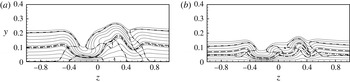
Figure 11. Lines of generalized inflection points in wall-normal direction within the boundary layer (— ⋅ ⋅ —), of sonic speed $(Ma=1)$ (— ⋅ —) and of $u+a=c_{ph}$ (— —) at $x=24$ for (a) case C-3DO-M, $c_{ph}=0.88$ (from § 4.1: tilt-even mode at $\unicode[STIX]{x1D714}_{r}=10$ ) and (b) case H-3DO-M, $c_{ph}=0.9$ . Thin solid lines are $u_{b}$ -isolines, starting with $u_{b}=0.1$ near the wall ( $\unicode[STIX]{x1D6E5}=0.1$ ), ending with $u_{b}=0.95$ .

The hot-flow case H-3DO-M shows the existence of two GIP lines along the entire spanwise extent. This is in accordance with the influence of wall cooling at the flat plate, see, e.g. Mack (Reference Mack1975). At the high-speed streak, case H-3DO-M does not show an inflection point. The line of $c_{ph}=u+a$ , with $c_{ph}\approx 0.9$ being a typical value for a second mode, is located significantly above the sonic line, compare case C-3DO-M.

Comparing cases H-3DO-M and H2-3DO-M slight differences can be found (not shown). The region of supersonic phase velocity above the wall is slightly larger for the stronger wall cooling. According to the smooth-plate linear stability theory this would mean that second-mode instabilities are more amplified in case H-3DO-M.

4.1 Identified unstable eigenmodes for $k=0.1$

Figure 12. Modulus of the B-LST perturbation amplitude (shading) at $x=24$ normalized by the maximum of the streamwise-velocity modulus. Case C-3DS-M: (a) streamwise velocity $|\hat{u} |$ , and (b) pressure $|\hat{p}|$ for even mode at frequency $\unicode[STIX]{x1D714}_{r}=3$ . Case C-3DO-M: (c,e) $|\hat{u} |$ and (d,f) $|\hat{p}|$ for tilt-even mode at $\unicode[STIX]{x1D714}_{r}=5$ and 10, respectively. Solid lines are $u_{b}$ -isolines. Dash-dot lines represent the sonic line. Symbols $\oplus$ and $\ominus$ describe an approximately opposite phase relation for the modulus maxima located beneath.

For cases C-3DS-M and C-3DO-M a detailed biglobal linear stability analysis has been carried out in a cross-plane at $x=24$ . The results reveal a multitude of unstable eigenmodes. For the two most unstable eigenmodes of each case, sections of the stability diagram have been computed by tracking the corresponding eigenvalues in the complex plane in terms of varying streamwise location $x$ and frequency $\unicode[STIX]{x1D714}_{r}$ . The investigated parameter space spans the intervals $16.5\leqslant x\leqslant 40$ and $0.5\leqslant \unicode[STIX]{x1D714}_{r}\leqslant 13$ , respectively. The base flow changes dramatically with $x$ in the near wake of the roughness. Therefore, the B-LST assumption of parallel flow may not be applicable, or its results may be doubtful. Comparing the maximum absolute values of the spatial gradients of case C-3DO-M in $(y{-}z)$ -cross-planes along $x$ reveals that within the examined streamwise range the streamwise gradient is at least one order of magnitude lower than the wall-normal or spanwise gradient. Thus, starting at $x=24$ the investigated eigenmodes are tracked also as far upstream as possible, until the correlation of the eigenmodes at consecutive streamwise locations becomes ambiguous.

Representative eigenfunction-amplitude distributions of the most unstable roughness-wake eigenmodes of cases C-3DS-M and C-3DO-M are shown in figure 12. In accordance with the phase relation of the dominant amplitude maxima, in case C-3DS-M the most unstable mode is an even mode (figure 12 a,b). The second most unstable mode is an odd mode (not shown) with a phase shift of about $\unicode[STIX]{x03C0}$ between both half-planes $z\gtrless 0$ . For case C-3DO-M the most unstable eigenmodes exhibit a similarity to the even and odd modes of case C-3DS-M, although the amplitude distributions are tilted. However, the corresponding phase relations of the eigenfunctions’ maxima reveal their even and odd nature. Therefore, the eigenmodes of case C-3DO-M shall be also referred to as tilt-even (figure 12 c,d) and tilt-odd mode. Note the existence of non-negligible pressure amplitudes at the wall for the eigenmodes (figure 12 b,d), and that the local maxima are located above the sonic line, except for $\unicode[STIX]{x1D714}_{r}=10$ in case C-3DO-M.

4.2 Local and integral growth for $k=0.1$

In the following, stability diagrams are discussed that are gained by a procedure different from classical (monoglobal) LST analysis. Instead of picking the most unstable eigenvalue from the spectrum at each combination $(\unicode[STIX]{x1D6FC}_{r},x)$ , the tracked biglobal modes are taken, the tracking along $\unicode[STIX]{x1D6FC}_{r}$ or/and $x$ started at a reference combination $(\unicode[STIX]{x1D6FC}_{r,ref},x_{ref})$ , where the modes to be tracked are chosen. Finally, the results are plotted as $\unicode[STIX]{x1D714}_{i}=\unicode[STIX]{x1D714}_{i}(\unicode[STIX]{x1D714}_{r},x)$ , with the $\unicode[STIX]{x1D714}_{r}$ -values being no more equidistant but approximately proportional to $\unicode[STIX]{x1D6FC}_{r}$ . The $N$ -factors are calculated spatially, i.e. as $N=-\int \unicode[STIX]{x1D6FC}_{i}\,\text{d}x$ , with $\unicode[STIX]{x1D6FC}_{i}$ obtained by Gaster’s relation. For the even mode this method yields the diagrams shown in figure 13, with the smooth-plate diagram for monoglobal modes at $\unicode[STIX]{x1D6FE}_{r}=5.5$ as reference. The tracked biglobal modes are multispectral with respect to $\unicode[STIX]{x1D6FE}_{r}$ and there is no distinguished plane $z=\text{const.}$ for these cases. Comparing the growth rates as well as the $N$ -factor isolines in figure 13, the stronger instability is clearly for the oblique set-up.

Figure 13. Details from the temporal stability diagrams of (a) case C-3DS-M even mode, (b) case C-3DO-M tilt-even mode and (c) case C-REF for spanwise wavenumber $\unicode[STIX]{x1D6FE}_{r}=5.5$ . Shading (contour levels are identical for all cases) shows temporal growth rate $\unicode[STIX]{x1D714}_{i}$ . Solid lines represent $N$ -factor isolines with levels shown. Integration started at initial amplification downstream of the roughness for (a,b) and near the plate’s leading edge for (c).

Case C-3DS-M exhibits a similarity to case C-REF in terms of the occurrence of distinct low- and high-frequency maxima. For case C-3DO-M the distinction between low- and high-frequency instability mode is less pronounced. For cases C-3DO-M and C-3DS-M the streamwise range of high-frequency instability is much larger than for case C-REF. On the smooth plate the low- and high-frequency unstable regions are related to the first- and second-mode instabilities, respectively. For increasing Mach number these regions first approach each other and finally, near $Ma=4.8$ , merge to one single instability region under adiabatic-wall conditions, compare, e.g. Mack (Reference Mack, Fasel and Saric2000) and Eissler & Bestek (Reference Eissler and Bestek1996). This merging can be observed in case C-3DS-M. In the vicinity of the roughness the frequency range of the second-mode-associated instability region is shifted to lower values. Marxen et al. (Reference Marxen, Iaccarino and Shaqfeh2010) observed a similar behaviour near a two-dimensional roughness. However, for the latter the shift vanishes downstream the element, the stability properties of the smooth-plate flow are recovered. In the wake of a three-dimensional roughness the flow deformation persists much longer, and the smooth-plate properties are not recovered within the considered domain.

Compare the tilt-even-mode eigenfunctions of case C-3DO-M in the low- and high-frequency region in figure 12(c–f), respectively. In contrast to the former the latter shows an additional near-wall maximum for streamwise velocity as well as pressure below the sonic line which is virtually identical with this mode’s line of $u+a=c_{ph}$ , see figure 11(a) $0.2\leqslant z\leqslant 0.4$ . With the contraction of the region of supersonic phase velocity at the high-speed streaks the line of supersonic phase velocity encloses the near-wall amplitude maxima of the eigenmode. Furthermore, there is a phase shift between the pressure’s wall maximum and the shear-layer maximum very much like the wall-normal characteristics of the second mode on the smooth plate. Based on these properties the B-LST low- and high-frequency eigenmodes of the roughness wake may henceforth also be referred to as roughness-wake first- and second-mode instabilities, respectively. Note that high-frequency eigenmodes with the same properties have been found for case C-3DS-M with the even mode resembling the varicose mode VC of DeTullio & Sandham (Reference DeTullio and Sandham2015) in a Mach-6 boundary layer which they also associated with the smooth-plate second- or Mack-mode instability. As observed by these authors the largest amplification of this mode is shifted to lower frequencies compared to the smooth-plate second mode.

In general it is found that for cases C-3DS-M and C-3DO-M the even and tilt-even modes are more amplified than the odd and tilt-odd modes, respectively. However, at the end of the investigated streamwise domain, the growth rates approach those of the odd modes being more persistent. This corresponds to the stronger decay of the wall-normal gradient compared to the spanwise gradient of $u_{b}$ shown in figure 7(a) with the even and odd modes being associated with the former and latter, respectively. However, within the investigated streamwise range of the present work the tilt-even mode of case C-3DO-M gains the largest $N$ -factors. The second mode reaches $N=6.8$ for $\unicode[STIX]{x1D714}_{r}=10$ compared to $N=6.4$ for the first mode at $\unicode[STIX]{x1D714}_{r}=5$ . $N\approx 5$ has been found sufficient for transition to turbulence in wind-tunnel experiments under noisy conditions. The tilt-even mode gains $N=5$ at approximately $x=33$ , corresponding to $180k$ or $98\unicode[STIX]{x1D6FF}_{u}$ downstream of the roughness centre.

The comparison of original and doubled roughness spacing shows similar amplitude distributions. However, the spatial growth rates at $x=24$ are generally larger for the smaller spacing, with a 10 % increase for the dominant tilt-even mode. Therefore the present set-up with $\unicode[STIX]{x1D706}_{z}=4b_{r}$ is slightly more unstable than the flow with an isolated element, also due to stronger induced cross-flow, see again figure 7(c).

4.3 Comparison of stability properties for various $k$ at $\unicode[STIX]{x1D713}_{r}=45^{\circ }$

Figure 14. Spatial growth rates $\unicode[STIX]{x1D6FC}_{i}$ from B-LST as a function of frequency $\unicode[STIX]{x1D714}_{r}$ at streamwise position $x=24$ . Case C-3DO-S most amplified low-frequency mode (— ⋅ —), case C-3DO-M tilt-even mode (— —), and case C-3DO-L tilt-even mode (——). Case C-REF three-dimensional disturbance with spanwise wavenumber $\unicode[STIX]{x1D6FE}_{r}=5.9$ (— ⋅ ⋅ —).

The growth rates of the most amplified modes at $x=24$ , approximately 50 boundary-layer thicknesses downstream of the element, differ significantly in the cases shown, see figure 14. For case C-3DO-S the characteristic of $\unicode[STIX]{x1D6FC}_{i}=\unicode[STIX]{x1D6FC}_{i}(\unicode[STIX]{x1D714}_{r})$ is similar to that of the corresponding smooth-plate eigenmode which is shown for comparison; the maximum growth rate for the low-frequency first mode is approximately 30 % larger at the streamwise location shown. On the other hand it is only 30 % of the maximum growth rate of case C-3DO-M. Case C-3DO-L shows as expected the strongest growth, being 50 % larger in maximum than for case C-3DO-M. Contrary to cases C-3DO-S and C-3DO-M, case C-3DO-L does not exhibit a second local maximum related to the high-frequency second mode. Figure 14(a) reflects the behaviour already described above: with increasing roughness height the local amplification maxima for low- and high-frequency modes shift to higher, and lower frequencies, respectively, approach, and finally merge fully. This fusion of first and second mode can also be seen for case C-3DO-M somewhat further downstream, see the stability diagram in figure 13(b). Note that for case C-3DO-L the eigenfunctions corresponding to frequencies beyond the single amplification maximum exhibit the typical additional near-wall pressure maximum below the sonic line. Thus, the continuous transition from roughness-wake first to second mode takes place in the region of the amplification maximum. The first- and second-mode instability regions have merged inseparably.

The effect of atmospheric-flight conditions on the B-LST results is not shown but will be discussed based on DNS in § 5.5.

5.1 Response to point-source pulsing for $k=0.1$

To gain a general overview of the stability and (internal) ‘receptivity’ behaviour of the investigated flows the steady base flows are exposed to an unsteady disturbance pulsing, see § 2.2 and figure 2 in particular. The diameter of the disturbance-source hole is $2R=0.429$ . For comparison, the wavelength of the smooth-plate two-dimensional eigenmode $(\unicode[STIX]{x1D6FE}_{r}=0)$ is $\unicode[STIX]{x1D706}_{x}\approx 1.03$ and 0.54 for frequencies $\unicode[STIX]{x1D714}_{r}=5$ and 10, respectively.

Figure 15. Response of the base flow to point-source pulsing. The pulse consists of the first 50 harmonics of fundamental frequency $\unicode[STIX]{x1D714}_{r,0}=0.5$ . Shading: (a–d) amplitude of streamwise-velocity disturbance $u^{\prime }$ gained from temporal Fourier analysis, the neutral line (— —) connects the streamwise locations of first amplification; (e,f) the natural logarithm of $u^{\prime }$ normalized by its value at $x=13$ . Cases: (a) C-REF, (b) C-2D-M, (c,e) C-3DS-M, and (d,f) C-3DO-M. The solid vertical lines mark the roughness location $x_{r}=15$ .

The responses in terms of disturbance amplitudes from temporal Fourier analysis for the flows of cases C-2D-M, C-3DS-M, C-3DO-M as well as C-REF are shown in figure 15(a–d). Note that this is not a ‘standard’ $N$ -factor stability diagram since at each frequency the receptivity of the multitude of excited modes varies and possible decay of the disturbances along the streamwise direction is also included. Figure 15(a) shows the neutral line for the sum of superposed eigenmodes in the smooth-plate flow. $N$ -factors for the sum of modes can be calculated by relating the downstream amplitudes to the values at the neutral point. Figure 15(a–d) thus show the amplitude spectra that would be observed in a respective experimental set-up. The amplitudes can be scaled to the level of the forcing in the experiment within the regime of modal growth. Note that larger forcing amplitudes will lead to a decrease in the streamwise extent of the purely linear flow behaviour. The representation of the results in figure 15(e,f) eliminates the influence of receptivity and transient processes in the flat-plate flow upstream the roughness by normalizing the amplitudes of each excited frequency by its respective value at $x=13$ . The shown natural logarithm represents the $N$ -factor for the sum of modes displaying the influence of the roughness and its wake only.

Figure 15(a–d) show that regardless of the roughness shape the behaviour resembles the smooth-plate behaviour up to a short distance upstream of the roughness $(x\approx 13)$ . Right downstream of the excitation location the disturbance-amplitudes drop throughout the frequency range before they start to grow again. The drop is more pronounced for higher frequencies. For some frequencies, in the second-mode range in particular, the excitation occurs upstream of branch I of the smooth-plate stability diagram. Downstream of $x\approx 13$ the response varies with the roughness shape.

The behaviour of case C-2D-M is in accordance with Marxen et al. (Reference Marxen, Iaccarino and Shaqfeh2010), see their figure 17. They found that the two-dimensional roughness acts ‘as a disturbance amplifier with a limited bandwidth’. The stability properties in its far wake resume the smooth-plate behaviour. Therefore, the amplification in front of and damping along the roughness results in an offset with respect to the smooth-plate evolution. Within the low-frequency region $(\unicode[STIX]{x1D714}_{r}\lesssim 8)$ the net effect for the disturbances is negligible. For higher frequencies $(8\lesssim \unicode[STIX]{x1D714}_{r}\lesssim 13)$ it results in an amplitude gain, compare the amplitude levels in figure 15(a,b) right behind the roughness. For frequencies beyond that range $(\unicode[STIX]{x1D714}_{r}\gtrsim 13)$ the net effect is negative. They are only weakly amplified upstream of the roughness, and comparably damped strongly along the element.

The spectrum of case C-3DS-M in figure 15(c) shows strong growth for two frequency intervals related to the roughness-wake first and second mode. The largest disturbance amplitudes are gained within the low-frequency range for $\unicode[STIX]{x1D714}_{r}=3$ . This frequency also shows the largest integral amplification, see figure 15(e). Whereas case C-3DS-M exhibits a response whose shape compares qualitatively to case C-2D-M, case C-3DO-M shows increased growth, and growth at all throughout the whole investigated frequency spectrum in agreement with the results of the B-LST analyses. The amplitude spectrum in figure 15(d) is dominated by frequencies $\unicode[STIX]{x1D714}_{r}=3$ , 6, and 9.5 reaching a similar order of magnitude of approximately $10^{-3}$ at the end of the investigated streamwise range. Due to nonlinear interaction the amplitude of the mean-flow deformation $(\unicode[STIX]{x1D714}_{r}=0)$ gains $10^{-4}$ . Figure 15(f) reveals that the integral amplification in the near wake is largest for $\unicode[STIX]{x1D714}_{r}=9.5$ with the lower frequencies catching up to the end of the streamwise domain.

5.2 Comparison of DNS and B-LST results for $k=0.1$

For case C-3DO-M a comparison of B-LST $u^{\prime }$ - and $p^{\prime }$ -eigenfunctions for the tilt-even mode with the corresponding DNS disturbance-amplitude distributions, in general, shows good agreement. However, an excellent representation of the DNS amplitude is obtained for a superposition of the tilt-even and tilt-odd B-LST mode, see figure 16. The relative weights of tilt-even and tilt-odd mode are 0.615 and 0.385 for $\unicode[STIX]{x1D714}_{r}=5$ , and 0.69 and 0.31 for $\unicode[STIX]{x1D714}_{r}=10$ , respectively.

Figure 16. Comparison of normalized disturbance-amplitude distributions from DNS (shading) and B-LST (thick solid lines) at $x=24$ for case C-3DO-M. (a) $u^{\prime }$ and (b) $p^{\prime }$ yielded by superposition of tilt-even (relative weight 60 %) and tilt-odd (40 %) mode with phase shift adapted to DNS signal for $\unicode[STIX]{x1D714}_{r}=5$ . (c) $u^{\prime }$ and (d) $p^{\prime }$ yielded by superposition of tilt-even (69 %) and tilt-odd (31 %) mode for $\unicode[STIX]{x1D714}_{r}=10$ . Thin solid lines are isolines of $u_{b}$ , starting with $u_{b}=0.1$ near the wall ( $\unicode[STIX]{x1D6E5}=0.1$ ), ending with $u_{b}=0.95$ .

Figure 17. Comparison of amplitude growth of streamwise-velocity disturbance $u^{\prime }$ from DNS (lines) and B-LST (symbols) for case C-3DO-M. Blank and filled symbols show the B-LST results for tilt-even and tilt-odd mode, respectively. Frequencies $\unicode[STIX]{x1D714}_{r}=5$ (——, ▫), amplitudes from B-LST and DNS matched at $x=24$ , and $\unicode[STIX]{x1D714}_{r}=10$ (— —, ♢), amplitudes matched at $x=30$ .

Though the single-frequency DNS signal extracted by temporal Fourier analysis obviously contains more than the dominant eigenmode at non-negligible amplitude, the comparison of dominant B-LST eigenmode growth and DNS disturbance evolution in figure 17 shows excellent agreement downstream of $x\approx 22$ for the low frequency. Up to this location the wavy characteristic implies a transient-growth behaviour, where the true amplitude of the dominant low-frequency disturbance is masked by damped modes of identical frequency and similar amplitude values. The high frequency shows a comparable beating within the same region. A similar scenario has been observed by Marxen et al. (Reference Marxen, Iaccarino and Shaqfeh2010) downstream of a two-dimensional roughness. They showed that the beating is due to a superposition of the dominating eigenmode and an additional stable mode generated by the roughness itself. The additional modes involved in the present case could be extracted by applying a multimode decomposition, see, e.g. Tumin (Reference Tumin2007). However, here the transient behaviour is limited to a short streamwise extent downstream the roughness, and a detailed investigation of the transient growth in the roughness wake has been set aside.

In contrast to the low frequency, a weak beating with a large streamwise wavelength can be observed downstream of the region of transient growth. Its wavelength cannot be extracted from the DNS disturbance evolution since only one nodal point of the beating is found within the simulated domain at $x\approx 30$ . Assuming that tilt even and tilt-odd mode are the dominant waves of this beating the resulting streamwise wavelength can be estimated to $\unicode[STIX]{x1D706}_{beat}=2\unicode[STIX]{x03C0}/|\unicode[STIX]{x1D6FC}_{r,even}-\unicode[STIX]{x1D6FC}_{r,odd}|\gtrsim 70$ which is larger than the computational domain.

The amplitudes of B-LST and DNS for $\unicode[STIX]{x1D714}_{r}=10$ in figure 17 have been matched at the streamwise location of the beating’s nodal point. However, the amplitude growth is underpredicted by B-LST within the largest part of the shown streamwise extent. In this case the linear superposition of even and odd modes with similar amplitudes results in a disturbance growth faster than the growth of the most unstable mode itself, at least locally. A similar phenomenon has been observed by DeTullio et al. (Reference DeTullio, Paredes, Sandham and Theofilis2013) in a Mach-2.5 boundary-layer flow altered by an isolated roughness. Nevertheless, B-LST and DNS show a larger integral growth for the roughness-wake second-mode disturbance, $N=5.7$ for $\unicode[STIX]{x1D714}_{r}=10$ instead of $N=4.6$ for $\unicode[STIX]{x1D714}_{r}=5$ in $22\leqslant x\leqslant 40$ .

5.3 Influence of skewing angle for $k=0.1$

Figure 18(a) shows that the wake is dominated by low-frequency first-mode disturbances for case C-3DS-M as well as C-3DO-M which is only due to their larger amplitudes in front of the roughness, and the transient-growth behaviour in its near wake. Figure 18(b) reveals that the strong amplitude gain by the transient-growth behaviour is limited to the low-frequency range, see also figure 15(e,f). Case C-3DO-M shows larger local and integral growth up to the end of the domain, with the second-mode disturbances exhibiting larger growth rates than the first-mode ones (for $x>30$ ) in a much larger streamwise range, see again figure 15(f). At about $x=43$ the second-mode growth rate decreases below the first mode’s, but, contrary to case C-3DS-M, is still positive up to the end of the streamwise domain. The above observations are in accordance with the results from the B-LST analysis.

Figure 18. (a) Amplitude growth of streamwise-velocity disturbance $u^{\prime }$ . (b) Natural logarithm of the $u^{\prime }$ -amplitude normalized by its value at $x=13$ for the vicinity of the roughness. Cases: C-3DS-M ▫ for $\unicode[STIX]{x1D714}_{r}=3$ (——), $\unicode[STIX]{x1D714}_{r}=10$ (— —); C-3DO-M ♢ for $\unicode[STIX]{x1D714}_{r}=6$ (——), $\unicode[STIX]{x1D714}_{r}=9.5$ (— —), $\unicode[STIX]{x1D714}_{r}=1.5$ (— ⋅ —). The vertical lines mark the roughness location $x_{r}=15$ .

On a closer look the amplitude growth of frequency $\unicode[STIX]{x1D714}_{r}=6$ in figure 18(a) shows a slight kink at $x\approx 52$ for case C-3DO-M. It is even more pronounced for $\unicode[STIX]{x1D714}_{r}=5$ (not shown). This sudden increase in the growth rate can be associated with a change in the mode dominance from the tilt-even to the tilt-odd mode. A superposition of both modes, as it has already been done in § 5.2, shows that for $\unicode[STIX]{x1D714}_{r}=5$ the ratio of even- and odd-mode amplitude is approximately 3:1 at $x=35.3$ , then drops to 1:1 at $x=46$ and further to 2:3 at $x\approx 51.7$ where the conversion becomes visible in the amplitude evolution. The change of the dominant mode from tilt even to odd has also been predicted by B-LST showing larger growth for the tilt-odd mode downstream of $x\approx 34$ , and is in accordance with the results of Choudhari et al. (Reference Choudhari, Li, Chang, Norris and Edwards2012) who found a similar behaviour in the wake of a diamond-shaped roughness in a Mach-3.5 boundary layer. Additionally, there may be an energy transfer between even and odd mode which exhibit similar phase velocities of $c_{ph}=0.88$ and 0.86 at $x=24$ , respectively, and a maximum difference of 3 % throughout the domain investigated by B-LST, $16.5\leqslant x\leqslant 40$ .

Based on figures 15 and 18 it becomes clear that for identical disturbance excitation the stronger growth in the wake of the obliquely placed roughness causes earlier transition than in the symmetric set-up. The two cases compared yield the same roughness Reynolds numbers for every criterion, see again table 4. However, the orientation of roughness elements with high ratios of spanwise width and streamwise length induce significant cross-flow in the wake, and thus palpably influences the transition location in the important subcritical regime in hypersonic flow.

5.4 Various roughness heights $k$ for $\unicode[STIX]{x1D713}_{r}=45^{\circ }$

Figure 19. Response of the base flow to point-source pulsing with harmonics $1\leqslant h\leqslant 50$ of fundamental frequency $\unicode[STIX]{x1D714}_{r,0}=0.5$ . $u^{\prime }$ -amplitude (shading) over $x$ and $\unicode[STIX]{x1D714}_{r}$ from temporal Fourier analysis. (a) case C-REF, (b) case C-3DO-S, (c) case C-3DO-M, (d) case C-3DO-L, (e) case H-3DO-M, (f) case H-3DO-L. The vertical lines mark the roughness location $x_{r}=15$ .

To investigate the influence of the roughness height on the flow stability properties the base flows of cases C-3DO-S, C-3DO-M and C-3DO-L are exposed to the point-source pulsing. The respective response is shown in figure 19. The characteristic of case C-3DO-S is virtually similar to that of the smooth-plate flow of case C-REF. DeTullio et al. (Reference DeTullio, Paredes, Sandham and Theofilis2013) and DeTullio & Sandham (Reference DeTullio and Sandham2015) also found their small-roughness set-ups with $Re_{kk}=169$ at $Ma_{\infty }=2.5$ and $Re_{kk}=60$ at $Ma_{\infty }=6$ , respectively, to only slightly alter the stability properties of the flat-plate flow. As we do, they also conclude that in these cases transition to turbulence is most likely not driven by the isolated roughness.

The response of cases C-3DO-L, see figure 19(d), differs more strongly from the smooth-plate result than case C-3DO-M. The spectrum of unstable frequencies extends to higher values. But whereas for case C-3DO-M there are still distinct frequency ranges that can be assigned to first and second modes with the limit being at about $\unicode[STIX]{x1D714}_{r}=9$ , such a clear distinction is lost in case C-3DO-L showing a broad-band response which again is in accordance with the findings from the B-LST. It is also evident that the flow of case C-3DO-L exhibits the strongest disturbance growth with the mean-flow distortion $(\unicode[STIX]{x1D714}_{r}=0)$ reaching values greater than 10 % at the end of the computational domain where the flow becomes transitional.

The vicinity of the roughness again is dominated by low-frequency disturbances, see figure 20(a). They benefit from a higher amplitude level in front of the roughness and the amplitude boost due to the transient-growth behaviour which is more pronounced for case C-3DO-L. For the latter the $u^{\prime }$ -amplitude increases by a factor of three within $\unicode[STIX]{x0394}x=0.5=4k$ whereas in case C-3DO-M it increases by a factor of 2 within the same streamwise range.

Figure 20. (a) Amplitude growth of streamwise-velocity disturbance $u^{\prime }$ for case C-3DO-M: symbol (♢), frequencies $\unicode[STIX]{x1D714}_{r}=2$ (— —), $\unicode[STIX]{x1D714}_{r}=6$ (——), and $\unicode[STIX]{x1D714}_{r}=0$ ( $\cdots \cdots$ ); case C-3DO-L: symbol (▵), $\unicode[STIX]{x1D714}_{r}=2$ (— —), $\unicode[STIX]{x1D714}_{r}=7$ (——) and $\unicode[STIX]{x1D714}_{r}=0$ ( $\cdots \cdots$ ). (b) Maxima of the spanwise mean value of $w_{b}$ in $(y{-}z)$ -cross-planes for cases C-3DO-M (——), C-3DO-L (— —), H-3DO-M (— ⋅ —) and H-3DO-L (— ⋅ ⋅ —). The vertical lines mark the roughness location $x_{r}=15$ .

Within the following region of exponential growth higher frequencies show larger amplification rates, and, thus, earlier reach transition-relevant amplitude levels. For case C-3DO-M, $\unicode[STIX]{x1D714}_{r}=6$ exhibits the highest amplitude at the end of the computational domain, see figure 20(a). Whereas the disturbances of case C-3DO-M still behave linearly at $x=53.7$ reaching an $N$ -factor of approximately 9 with respect to the value at $x=13$ , for case C-3DO-L the frequency $\unicode[STIX]{x1D714}_{r}=7$ gains $N=10$ already at about $x=40.3$ and goes into nonlinear saturation at $x\approx 44.5$ with a $u^{\prime }$ -amplitude of approximately 2 %. Starting from lower amplitude levels frequencies $7<\unicode[STIX]{x1D714}_{r}\leqslant 11$ show even larger integral growth for $13\leqslant x\leqslant 40$ . $\unicode[STIX]{x1D714}_{r}=10.5$ reaches $N=10$ first at $x=38.5$ .

The strong kink in the disturbance-amplitude evolution for $\unicode[STIX]{x1D714}_{r}=2$ at about $x=38.5$ is a direct consequence of the nonlinear generation of very-low-frequency modes including a three-dimensional mean-flow distortion, see also figure 19(d), that both drive the amplitudes of disturbances with higher frequencies within the low-frequency band. (We found a strongly similar behaviour for subsonic flow cases without roughness with a broad initial disturbance spectrum.) From this location on, nonlinear generation dominates the amplitude growth of low frequencies. Downstream of a kink the maxima of the disturbance-amplitude distribution virtually collapse with the extrema of the mean-flow distortion. Toward the end of the computational domain the flow of case C-3DO-L becomes transitional with the whole frequency spectrum reaching amplitudes larger than 1 %, see figure 19(d).

5.5 Effect of atmospheric-flight conditions

The point-source pulsing is also applied to the hot-flow cases. The response is shown in figure 19(e,f) for cases H-3DO-M and H-3DO-L, respectively. The fundamental frequency $\unicode[STIX]{x1D714}_{r,0}=0.5$ corresponds to a dimensional value of $\tilde{\unicode[STIX]{x1D714}}_{r,0}/(2\unicode[STIX]{x03C0})=6.73$  kHz instead of 4.55 kHz for the cold-flow conditions. Though for cold- and hot-flow cases the amplitudes drop to comparable levels right downstream of the excitation location due to receptivity properties, the disturbance growth of the hot-flow case is weaker upstream the roughness. The first-mode amplification is strongly reduced due to wall cooling, whereas the second mode is shifted to higher frequencies due to the reduced boundary-layer thickness. Thus, the frequency gap between amplified first and second mode is much larger for the hot flow.

Based on figure 19 it can be observed that, in general, the amplitude growth is weaker for the hot cases comprising smaller bands of amplified frequencies, at least in the near wake of the roughness, which implies a similarity to the smooth-plate behaviour described above. The less pronounced instability of the hot-flow cases may also be attributed to the slightly lower streak amplitude, see figure 10(a), whereas wall-normal and spanwise gradients of the streamwise base-flow velocity obviously are even larger for the hot-flow cases. The final amplitude levels of cases C-3DO-M and H-3DO-L are comparable, the latter having the broader frequency band. Note that these cases also show a comparable cross-flow magnitude, see figure 20(b).

Thus, it becomes clear that case C-3DO-L is the most critical in terms of earlier transition. Compared to case H-3DO-L, the frequency band fills up earlier and more evenly to nonlinear amplitude levels. In case H-3DO-L the gap between first and second modes is still visible when the nonlinear generation of the base-flow distortion $(\unicode[STIX]{x1D714}_{r}=0)$ starts at $x\approx 42$ .

Figure 21. (a) Amplitude growth of streamwise-velocity disturbance $u^{\prime }$ for case C-3DO-L (▫), frequencies $\unicode[STIX]{x1D714}_{r}=2$ (— —), $\unicode[STIX]{x1D714}_{r}=7$ (——) and case H-3DO-L (○), $\unicode[STIX]{x1D714}_{r}=1.5$ (— —), $\unicode[STIX]{x1D714}_{r}=4.5$ (——). Base-flow distortion is given by $\unicode[STIX]{x1D714}_{r}=0$ ( $\cdots \cdots$ ). The vertical line marks the roughness location $x_{r}=15$ . Normalized DNS disturbance-amplitude distribution (shading) of $u^{\prime }$ at $x=36$ for (a) case C-3DO-L at $\unicode[STIX]{x1D714}_{r}=7$ and (b) case H-3DO-L at $\unicode[STIX]{x1D714}_{r}=4.5$ . Thin solid lines are isolines of $u_{b}$ , starting with $u_{b}=0.1$ near the wall ( $\unicode[STIX]{x1D6E5}=0.1$ ), ending with $u_{b}=0.95$ .

Nevertheless, the amplitude development of the most amplified frequencies in the near wake and the far wake, respectively, in figure 21(a) reveals an interesting fact: compared to the cases with $Re_{kk}=434$ , where the amplitude growth is stronger in general for the cold flow, here growth rates are at comparable levels for distinct frequencies. The growth rates of $\unicode[STIX]{x1D714}_{r}=7$ in case C-3DO-L and $\unicode[STIX]{x1D714}_{r}=4.5$ in case H-3DO-L are virtually identical within $25\lesssim x\lesssim 35$ . In the near-wake the first-mode low-frequency disturbance is even more amplified in case H-3DO-L. However, the respective high-frequency but also first-mode disturbances are again dominant towards the end of the computational domain with case C-3DO-L reaching the nonlinear amplitude levels earlier than case H-3DO-L. The overall integral growth in terms of an $N$ -factor for the sum of modes with respect to the amplitude at $x=13$ shows $N=10$ at $x=40.3$ for $\unicode[STIX]{x1D714}_{r}=7$ in case C-3DO-L, as already mentioned above. This corresponds to $138\unicode[STIX]{x1D6FF}_{u}$ at $x_{r}=15$ . In case H-3DO-L frequency $\unicode[STIX]{x1D714}_{r}=4.5$ exhibits $N=10$ at approximately $x=43.8$ or $229\unicode[STIX]{x1D6FF}_{u}$ . The similar stability behaviour of cases C-3DO-L and H-3DO-L for distinct frequencies may be attributed to the similar streak amplitude, see figure 10(b). On the other hand, wall-normal and spanwise gradients of the streamwise base-flow velocity are larger and the cross-flow is weaker in case H-3DO-L.

Though growth rates of the most amplified disturbance frequencies are comparable for cases H-3DO-L and C-3DO-L, the mean-flow distortion growth is weaker in the hot flow, see again figure 21(a). This likely is due to the less pronounced mode interaction since the amplitude levels of the involved frequencies are less evenly distributed within the spectrum. Figure 21(b,c) compare the amplitude distributions of the integrally most amplified high-frequency first-mode disturbances. As can be expected from the differences in the base flows their shape is quite different.

The above observations oppose the transition criteria of Bernardini et al. (Reference Bernardini, Pirozzoli and Orlandi2012) and Bernardini et al. (Reference Bernardini, Pirozzoli, Orlandi and Lele2014) which, at identical values of $Re_{kk}$ , evaluate the hot-flow cases with wall cooling as more critical, see table 4. The present results reproduce the trend given by the criterion of Redford et al. (Reference Redford, Sandham and Roberts2010) showing stabilization by wall cooling. Nevertheless, the criteria of Bernardini et al. (Reference Bernardini, Pirozzoli and Orlandi2012) and Bernardini et al. (Reference Bernardini, Pirozzoli, Orlandi and Lele2014) still might hold for symmetric roughness configurations. In the asymmetric cases compared here, the respective hot flows show lower cross-flow magnitudes at identical $Re_{kk}$ , see again figure 20(b).

The differences in disturbance evolution are small comparing cases H-3DO-M and H2-3DO-M. For the respective emissivities $\unicode[STIX]{x1D716}=0.8$ and 0.6 of the radiation adiabatic wall the smooth-wall temperature at $x_{r}=15$ differs by approximately 5 %, see table 2. Nevertheless, the trend that can be observed in the comparison of roughness-wake first- and second-mode disturbance growth in figure 22 resembles the well-known behaviour of the smooth-wall flow. Wall cooling stabilizes the first-mode instabilities (figure 22 a), and destabilizes the second-mode ones (figure 22 b). Though, here, the destabilization of the second mode must be accounted to a larger streamwise range of amplification at virtually identical maximum growth rates.

Figure 22. Natural logarithm of the $u^{\prime }$ -amplitude normalized by its value at $x=13$ for cases H-3DO-M (▿) and H2-3DO-M (▵) for frequencies (a) $\unicode[STIX]{x1D714}_{r}=1$ (— —), $\unicode[STIX]{x1D714}_{r}=2.5$ (——) and (b) $\unicode[STIX]{x1D714}_{r}=12$ (——) and $\unicode[STIX]{x1D714}_{r}=13$ (— ⋅ —). Note the different scales. The vertical lines mark the roughness location $x_{r}=15$ .

DeTullio & Sandham (Reference DeTullio and Sandham2015) observed a different behaviour for their second-mode-like instability (mode VC) based on a wall-temperature reduction from the adiabatic value to 50 % of it. This change showed only small influence on the low-frequency first-mode instabilities in the wake of the square-box roughness, but showed a reduction of 33 % for the maximum growth rate of the wake mode VC. Note that DeTullio & Sandham (Reference DeTullio and Sandham2015) adapted their global simulation Reynolds number to yield the identical $Re_{kk}$ instead of reducing the roughness height. The impact of the rather strong change in the thermal boundary condition on the base flow is not shown by the authors.

5.6 Nonlinear disturbance evolution in the transitional flow regime for case C-3DO-M

To gain a better understanding of the transition onset downstream of the obliquely placed roughness of case C-3DO-M the frequency content of the pulsing is reduced to a biharmonic point-source excitation involving $\unicode[STIX]{x1D714}_{r}=5$ and 10. According to the above analysis these represent a first-mode and a second-mode instability, respectively. The excitation amplitude is increased to $(\unicode[STIX]{x1D70C}v)_{max,h}^{\prime }=10^{-4}$ for each frequency in order to make sure that on one hand the disturbance evolution starts within the linear regime and on the other hand transition occurs within the investigated computational domain. Phase shifts $\unicode[STIX]{x1D703}_{h}$ are again set to zero. The chosen numerical resolution for the simulation yields worst-case values of $(\unicode[STIX]{x0394}x^{+},\unicode[STIX]{x0394}y_{min}^{+},\unicode[STIX]{x0394}z^{+})\approx (4.4,0.55,2.2)$ in the turbulent region at the end of the computational domain which are comparable to the resolution chosen for the breakdown scenario in DeTullio & Sandham (Reference DeTullio and Sandham2015). The following results are based on a temporal Fourier analysis with a fundamental frequency of $\unicode[STIX]{x1D714}_{r,0}=2.5$ . Thus, $\unicode[STIX]{x1D714}_{r}=5$ and 10 correspond to harmonics $h=2$ and 4, respectively, and the first subharmonic of the lower excitation frequency can be resolved.

Figure 23. Case C-3DO-M: (a) comparison of streamwise-velocity disturbance amplitudes $u^{\prime }$ for excitation amplitudes $(\unicode[STIX]{x1D70C}v)_{max,h}^{\prime }=10^{-4}$ (lines) and $10^{-7}$ (symbols), respectively, for $\unicode[STIX]{x1D714}_{r}=5$ (——), (♢) and $\unicode[STIX]{x1D714}_{r}=10$ (— —), (▫) and $\unicode[STIX]{x1D714}_{r}=0$ (— ⋅ —). The data for $(\unicode[STIX]{x1D70C}v)_{max,h}^{\prime }=10^{-7}$ have been scaled with $10^{3}$ . The vertical lines mark the roughness location $x_{r}=15$ . (b) Phase velocities from B-LST for the dominant eigenmodes. Tilt-even mode (——) and tilt-odd mode (— ⋅ —) at $\unicode[STIX]{x1D714}_{r}=5$ , and tilt-even mode (— —) and tilt-odd mode (— ⋅ ⋅ —) at $\unicode[STIX]{x1D714}_{r}=10$ .

According to the comparison of the $u^{\prime }$ -amplitude evolution along $x$ for the excitation with $(\unicode[STIX]{x1D70C}v)_{max,h}^{\prime }=10^{-4}$ and that of the linear analysis above with $10^{-7}$ scaled with the missing factor of $10^{3}$ in figure 23(a), the streamwise amplitude growth is virtually identical for both excited frequencies up to about $x=33$ . At $x=32.7$ the three-dimensional mean-flow deformation reaches a $u^{\prime }$ -amplitude of 0.5 %, see figure 24. The following deviation from the purely linear behaviour of the disturbance growth involving nonlinear interaction results in saturation of the amplitudes at levels larger than 10 %.

Figure 24. Case C-3DO-M: (a) amplitude spectrum for streamwise-velocity disturbance $u^{\prime }$ for the biharmonic point source with amplitude $10^{-4}$ , gained from temporal Fourier analysis. (b) $u^{\prime }$ -amplitude growth for $\unicode[STIX]{x1D714}_{r}=5$ (——), $\unicode[STIX]{x1D714}_{r}=10$ (— —) and mean-flow deformation $\unicode[STIX]{x1D714}_{r}=0$ (— ⋅ —). Additionally, even (— —) and odd harmonics $(\cdots \,)$ of fundamental frequency $\unicode[STIX]{x1D714}_{r,0}=2.5$ are shown. The vertical lines mark the roughness location $x_{r}=15$ .

Figure 24(a) shows the response to the disturbance excitation for the complete frequency spectrum in terms of $u^{\prime }$ -amplitude. The start of the nonlinear generation of the (three-dimensional) mean-flow deformation $(\unicode[STIX]{x1D714}_{r}=0)$ at approximately $x\approx 21$ is visible in the Fourier data by a sudden increase in growth rate. Near this location the amplitude of $\unicode[STIX]{x1D714}_{r}=5$ exceeds $10^{-3}$ . Starting from lower amplitude levels but experiencing virtually identical amplification, the generation of even harmonics of $\unicode[STIX]{x1D714}_{r,0}=2.5$ which are the harmonics of the excited frequencies, can be observed in figure 24(b). Their amplitude levels at a distinct streamwise location $x$ are staggered by increasing frequency due to the successive generation of higher harmonics. Shortly downstream of $x=39.5$ , where the mean-flow deformation reaches a $u^{\prime }$ -amplitude of approximately 10 %, all even harmonics run into saturation. At $x\approx 35$ , the mean-flow deformation reaches the amplitude level of $\unicode[STIX]{x1D714}_{r}=10$ and lowers the growth of the latter compared to its exponential growth behaviour in figure 23(a); slightly downstream the low-frequency mode gets an amplitude boost, indicating an enhanced energy transfer from the distorted mean flow. The flow eventually reaches a transitional state, and generation of odd harmonics is initiated which gain comparable amplitude levels at the end of the computational domain.

Figure 25. Case C-3DO-M snap-shot visualization: perspective view of vortex structures by means of the $\unicode[STIX]{x1D706}_{2}$ -criterion ( $\unicode[STIX]{x1D706}_{2}=-0.07$ ). Shading indicates wall-normal distance $y$ .

Figure 26. Case C-3DO-M snap-shot visualization: (a) top view and (b) side view of vortex structures by means of the $\unicode[STIX]{x1D706}_{2}$ -criterion ( $\unicode[STIX]{x1D706}_{2}=-0.07$ ). Shading indicates (a) wall-normal distance $y$ and (b) velocity $u$ . (c) pressure at the wall $p_{w}$ . (d) Skin friction coefficient $c_{f}$ based on velocity $u$ . Note that axes are not to scale.

Figure 27. Details of figure 26(a,b) with shading for identical quantities at identical levels. Note that for (b) axes are not to scale.

Figures 25 and 26(a,b) show a snap-shot of the flow in terms of vortex structures visualized by means of the $\unicode[STIX]{x1D706}_{2}$ -criterion, and figure 26(c,d) the pressure at the wall and the skin friction coefficient. The longitudinal vortex system originating at the roughness and its decay in the wake are visible as well as the first unsteady disturbances at the leading-edge main vortex at approximately $x=24$ . Figure 26(b) clearly shows localized vortex structures in the direct line of the steady wake vortex, $27.5\leqslant x\leqslant 36$ , with a large wavelength indicating the effect of the low-frequency mode, cf. figure 16(a), most near-wall structure. See also figure 27 for details. For $x>30$ the high-frequency mode is visible above with half the wavelength. Looking at figure 16(a,c) for the respective eigenmode shapes it becomes clear that there must be constructive and destructive interference for the far-wall and near-wall structure of the two frequencies, respectively, visible in figure 26(a,b), supported by a nonlinear coupling. With the disturbances reaching amplitudes of roughly 5 % near $x=36$ subsequent interaction of induced vortical structures can be observed. For $38\leqslant x\leqslant 45$ the low-frequency disturbances with their larger wavelength dominate again, see figure 26(a). Downstream of approximately $x=45$ the start of their breakdown to increasingly smaller scales and the formation of a turbulent wedge is evident. The lift-up of the vortices, and the sudden increase in boundary-layer thickness coinciding with the breakdown of the large vortex structures can be observed. Note that the evolution of the disturbance structures takes place off centre since it is bound to the spanwise position of the dominant low-speed streak. The finest structures can be found on top of the latter. In terms of spanwise location the earliest onset of fluctuation growth is found near $z=0.05$ where the superposition of the dominant eigenmodes of the involved frequencies exhibit a local maximum in their amplitude distribution.

In between the evolving turbulent wedges, occurring periodically in spanwise direction, an oblique near-wall wave pattern can be observed which makes the turbulent wedge look fishbone-like in the top view of the vortex structures, see again figure 26(a). The propagation direction of these waves with respect to the $z$ -direction differs dependent on the half-plane $(z\gtrless 0)$ they are moving in. Near the spanwise boundaries of the computational domain, where periodicity is prescribed, the waves from both half-planes interfere. From the pressure distribution at the wall in figure 26(c) the streamwise and spanwise wavenumbers can be measured to $\unicode[STIX]{x1D6FC}_{r}\approx 9.6$ and $\unicode[STIX]{x1D6FE}_{r}\approx 4.9$ . Based on an estimation for the phase velocity from the LST results for the corresponding smooth-plate flow, $c_{ph}\approx 0.92$ for $\unicode[STIX]{x1D6FE}_{r}\approx 5.5$ , the frequency of these waves is approximately $\unicode[STIX]{x1D714}_{r}=8.8$ . Since the flow outside the direct wake is still smooth-plate like, the observed waves are three-dimensional smooth-wall oblique second-mode instabilities excited by the high-frequency roughness-wake mode, cf. figure 13(c).

For the following analysis the flow data have been averaged over 18 time periods of the lower disturbance excitation frequency $\unicode[STIX]{x1D714}_{r}=5$ . The doubling of the number of periods for averaging yields the same results. The mean values of time are marked with $\overline{\unicode[STIX]{x1D719}}$ . The spanwise averaging has been restricted to the range with turbulent appearance $0.05\leqslant z\leqslant 0.3$ at the end of the computational domain. For comparison the spanwise average for the complete domain is shown.

Figure 28. Case C-3DO-M: (a) local skin friction coefficient $c_{f}$ with respect to $\langle \overline{u}\rangle$ . Spanwise averaging for $-1.6\leqslant z<1.6$ (— —) and $0.05\leqslant z\leqslant 0.3$ (——); laminar smooth-plate solution (— ⋅ —) and values for turbulent flow (— ⋅ ⋅ —). (b) Maximum over $y$ and $z$ of $tke$ (— —) and volume integral of $I_{tke}(x)$ (——). (c) Van Driest transformed $\overline{u}$ -profile normalized by wall shear velocity $u_{vD}^{+}$ at $x=53$ . Spanwise averaging as in (a); $u^{+}=y^{+}$ (— ⋅ —), $u^{+}=0.38^{-1}\ln y^{+}+4.1$ (— ⋅ ⋅ —), and results for a turbulent Mach-4.5 flat-plate flow from Jiang et al. (Reference Jiang, Choudhari, Chang and Liu2006), symbols (▫).

In figure 28(a) the strong increase of the mean skin friction coefficient $c_{f}$ , which commonly is used to signal the onset of transition, starts at approximately $x=40.5$ . It correlates well to the streamwise region where the disturbance amplitudes of the excited frequencies reach their saturation level, compare figure 24(b). The same holds for the maximum of the turbulent kinetic energy $tke=0.5(\overline{{u^{\prime }}^{2}}+\overline{{v^{\prime }}^{2}}+\overline{{w^{\prime }}^{2}})$ in streamwise cross-planes, see figure 28(b). The volume integral $I_{tke}(x)=\int _{x_{1}}^{x}\int _{y_{1}}^{y_{2}}\int _{z_{1}}^{z_{2}}(tke)\,\text{d}\unicode[STIX]{x1D701}\,\text{d}\unicode[STIX]{x1D702}\,\text{d}\unicode[STIX]{x1D709}$ starts to deviate from the exponential growth behaviour upstream. Downstream, $c_{f}$ shows the overshoot typical for the transitional regime and afterwards oscillates around the skin friction relation for a compressible turbulent flat-plate boundary layer as given by White (Reference White2006), equation 7-132. The oscillation is likely due to the intermittent state of the turbulence in this still transitional region. The rise in $c_{f}$ is moderate for the complete-domain spanwise averages due to the large fraction of laminar flow. The offset with respect to the laminar smooth-plate solution that is evident within the fully laminar region of the flow for $18<x<40$ results from the base-flow high-speed streaks caused by the trailing vortices.

Figure 29. Case C-3DO-M: (a) perspective view of time-averaged turbulent kinetic energy by means of an isosurface at $tke=0.003$ with isolines of time-averaged streamwise velocity $\overline{u}$ in cross-planes at $x=38.2$ and 42.4 are shown, starting with $\overline{u}=0$ at the wall ( $\unicode[STIX]{x1D6E5}=0.1$ ), ending with $\overline{u}=0.95$ . Note that axes are not to scale. Circles indicate starting points of turbulent spreading. Coordinates of point 1 $(x,y,z)=(38.2,0.32,0.30)$ with $\overline{u}=0.78$ . Point 2 $(41.1,0.15,0.04)$ with $\overline{u}=0.85$ . Point 3 $(42.4,0.09,-0.10)$ with $\overline{u}=0.88$ . (b) Pressure at the wall comparing DNS (shading) and the reconstruction based on the four dominant B-LST eigenmodes (solid lines).

As mentioned above the onset of transition is commonly detected based on a strong increase of the skin friction coefficient $c_{f}$ . Actually, transition does not start at the wall but above with the distance depending on Mach number as described in Fischer (Reference Fischer1972). This phenomenon has been called ‘precursor transition’ by Pruett & Zang (Reference Pruett and Zang1992). For high Mach numbers the point where turbulence is initiated is located near the boundary-layer edge. It roughly coincides with the so-called critical layer $c_{ph}=u_{b}$ , where responsible instability modes exhibit amplitude maxima. From its ‘starting point’ the turbulence spreads in wall-normal and spanwise directions forming the turbulent wedge. The initial formation of such a wedge can be seen in figure 29(a) showing an isosurface of time-averaged $tke$ . Figure 28(b) shows the streamwise evolution of the $tke$ in terms of its specific maximum value occurring in streamwise cross-planes as well as its integral value. Both show exponential growth downstream of the roughness up to the location where the breakdown starts. Interestingly, the isosurface of $tke$ shows several streamwise starting points at various spanwise and wall-normal locations. All these points are located near the local boundary-layer edge. The most upstream of these points can be found where the low-speed streak shows its maximum wall-normal extent in the corresponding $(y{-}z)$ -cross-plane. This region correlates to the locations of the local maxima in the disturbance-amplitude distributions of the excited frequencies. As already mentioned above, the region where the finest vortex structures can be observed lies directly downstream. For the marked points in figure 29(a) $\overline{u}$ roughly differs between 0.78 and 0.88 and, thus, is close to the phase velocities of the involved eigenmodes showing $0.875\leqslant c_{ph}\leqslant 0.90$ at $x=38$ , see figure 23(b).

Fischer (Reference Fischer1972), investigating turbulent wedges formed behind isolated roughness specks, found that the spreading angle towards the wall ‘seems to remain essentially invariant with Mach number’. DNS results from Pruett & Zang (Reference Pruett and Zang1992) for axisymmetric boundary layers at $Ma=4.5$ and 6.8, and Sivasubramanian & Fasel (Reference Sivasubramanian and Fasel2015) for $Ma=6$ support this finding. The spanwise spreading angle on the other hand strongly decreases with Mach number. In the present case both spreading angles were evaluated based on the isosurface of time-averaged $tke$ shown in figure 29(a). The spanwise angles with respect to the $x$ -axis differ at both sides showing about $3.5^{\circ }$ in negative and $2.4^{\circ }$ in positive $z$ -direction. Since only the initial formation of the turbulent wedge is observed these values surely are subject to inaccuracy. Nevertheless, they quite well correspond to the trend given in Fischer (Reference Fischer1972), with a spreading angle between approximately $2.6^{\circ }$ and $4^{\circ }$ . A similar estimation for the spreading angle in wall-normal direction starting from point 1 in figure 29(a) yields an angle of about $1^{\circ }$ . This value agrees with the findings of Pruett & Zang (Reference Pruett and Zang1992), $1^{\circ }$ for the axisymmetric Mach-4.5 case, as well as the approximate value of about $0.6^{\circ }$ given by Fischer (Reference Fischer1972). Hence, the turbulent-wedge evolution in the streak-induced breakdown with a roughness element is similar to the breakdown without discrete roughness, where the oblique-type breakdown with self-induced streaks typically plays a dominant role.

Figure 28(c) shows the van Driest transformed velocity profiles at the end of the computational domain. The transformation has been carried out according to White (Reference White2006), equation 7-107. The change towards the turbulent profile becomes evident though it is not yet fully developed, particularly to be seen near the boundary-layer edge. The inner layer appears to be developed up to $y^{+}=50$ which corresponds to $y\approx 0.2$ . For a fully developed turbulent boundary layer the log-law $u_{vD}^{+}\approx c_{1}^{-1}\ln y^{+}+c_{2}$ holds within the inner layer. White (Reference White2006) proposes $c_{1}\approx 0.41$ and $c_{2}\approx 5$ . For the results shown in figure 28(c) the agreement is better for the values $c_{1}\approx 0.38$ and $c_{2}\approx 4.1$ found by Österlund et al. (Reference Österlund, Johansson, Nagib and Hites2000). This is in agreement with Jiang et al. (Reference Jiang, Choudhari, Chang and Liu2006), who investigated a turbulent Mach-4.5 flat-plate boundary layer, and Stolz & Adams (Reference Stolz and Adams2003).

Figure 30. Perspective views of the vortex structures by means of isosurfaces of $\unicode[STIX]{x1D706}_{2}=-0.05$ for $32\leqslant x\leqslant 35.5$ from (a) DNS and (b) the reconstruction based on the four dominant B-LST eigenmodes. The shading indicates the wall-normal coordinate $y$ .

Encouraged by the very good agreement between the amplitude distributions from DNS and B-LST, the three-dimensional disturbance evolution of the present case is reconstructed based on the B-LST results from § 4 and information about amplitudes and phase shifts of the involved modes from DNS. For both excited frequencies only the tilt-even and tilt-odd mode are taken into account. The comparison of the resulting vortex structures and pressure distribution at the wall are shown in figures 30 and 29(b), respectively. The general agreement between DNS and B-LST is very good. Non-parallel effects, see Bonfigli & Kloker (Reference Bonfigli and Kloker2007) for a three-dimensional incompressible boundary layer with cross-flow vortices, play a minor role for the present B-LST analysis of the flow with streaks having eventually vanishing streamwise vorticity.