4.1. Thin film evolution and disturbance onset

Figure 2 shows the validation experimental and simulation data associated with the dynamical evolution of a Triton X-100 aqueous film over an air bubble. The experimental conditions and experimental parameters are presented in table 1 with $t_{stop} = 3.11$. Figure 2(a) shows the temporal evolution of the maximum film thickness. For the experimental data, $\hat {h}_{max}$ is defined to be the maximum measurable film thickness within the field of view, while in the simulation, $\hat {h}_{max} = \max (\hat {h}(t, r \leqslant R(\theta ), \theta ))$, where $R(\theta )$ corresponds to the radial position of minimum film thickness for a given azimuthal direction. Here $R(\theta )$, the rim, bounds the so-called dimple.

Figure 2. Evolution of a Triton X-100 aqueous film over an air bubble. (a) Dynamics of the maximum film thickness measured in the experiment (circles) and obtained via 2-D numerical simulation (solid line). The experimental parameters and simulation parameters are reported in table 1, with a $t_{stop} = 3.11$. The twelve filled circles correspond to the twelve interference patterns displayed in (b). The diameter for each of the interferograms corresponds to 1.2 mm. The location of $\hat {h}_{max}$ is marked with an ‘x’.

In both the experiment and the simulation, $\hat {h}_{max}$ decreases with time as a result of the squeezing motion of the motor driving the two interfaces together. Similar to the experiments done by Frostad et al. (Reference Frostad, Tammaro, Santollani, de Araujo and Fuller2016), this experiment also shows three stages of film evolution. The first stage corresponds to the time when the motor is moving: $0 < t < t_{stop}$. During this period, the bubble is forced upward and the dimple grows from $r = 0$ radially outward in an axisymmetric fashion (figure 2b1–3). The second stage corresponds to the rapid change in film thickness after $t_{stop} = 3.11$ ($t_{stop} < t < 5$, figure 2b4–10). Figure 3(a) provides the film thickness contour that corresponds to the interference pattern in figure 2(b4). Shortly after the motor has stopped moving, the system succumbs to ambient disturbances that break the axial symmetry of the outermost blue ring that corresponds to the rim location (figure 2b5). Figure 3(b) shows the effect of the disturbances on the film thickness at $t = 3.65$. As the amplitude of the disturbance grows, the thin film becomes more asymmetrical, and the previously centred $\hat {h}_{max}$ is convected away from $r = 0$ (figures 2b6–8 and 3c). Eventually, the dimple discharges from the side (figure 2b9 and 2b10), leaving behind a plume of a very non-axisymmetric film (figure 2b11 and 2b12). The film enters the last stage of its evolution, where the non-axisymmetric film continues to thin at a rate that is slowed relative to that during the dimple discharge (figure 2a). The bubble eventually coalesces as a result of further ambient disturbances.

Figure 3. Experimental film thickness profiles during the symmetry breaking event for an aqueous solution of Triton X-100 at a concentration of 0.01 mM; (a) $t = 3.47$, (b) $t = 3.65$, (c) $t = 3.83$. These contour maps correspond to the interference patterns presented in figures 2(b4), (b5) and (b6).

In contrast to the experimental evolution of $\hat {h}_{max}$, the simulated maximum film thickness thins at a faster rate during $0 < t < 1$, leading to a thinner film during $1 < t < 4.22$. We believe the differences are mainly the result of our assumption that the lower surface is non-deformable. This assumption can be evaluated by examining the deformation of a freely rising bubble in a surfactant free liquid (Pigeonneau & Sellier Reference Pigeonneau and Sellier2011). The Bond number in this study is close to the parameter used in figure 9(a) of Pigeonneau & Sellier (Reference Pigeonneau and Sellier2011), where an air bubble freely rises toward an initially flat liquid–air interface with a one-radius initial clearance over the apex of the bubble. In their study, a small amount of deformation is observed when the bubble freely rises until the minimum film thickness approaches the numerical resolution. In fact, Pigeonneau & Sellier (Reference Pigeonneau and Sellier2011) have deemed the deformation to be small enough such that ‘the bubble remains nearly spherical when rising’. However, in our study, a motor forces the bubble upward, thus moving beyond the position described in figure 9(a) of Pigeonneau & Sellier (Reference Pigeonneau and Sellier2011). It is possible that the actual bubble deformation exceeds that reported by Pigeonneau & Sellier (Reference Pigeonneau and Sellier2011). Furthermore, due to the limitations in the azimuthal mesh size, the simulation can capture the evolution of the film up to $t = 4.22$, at which time the accumulated numerical round-off errors act to disturb the rim. Despite the limitations of the numerical tool, we can still capture the onset of the symmetry breaking event. Understanding the underlying physics that drives the symmetry breaking is the first step to understanding the subsequent rapid dimple discharge that affects the overall bubble lifetime. For the remainder of this paper, we focus on understanding the onset of symmetry breaking as shown in figures 2(b5) and 3(b).

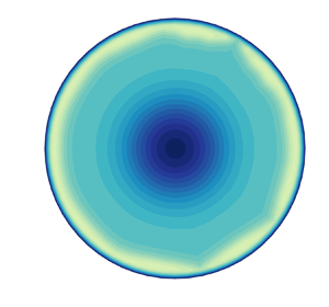
Figure 4 provides the onset of symmetry breaking observed in the two-dimensional (2-D) simulation. At $t = 4.10$, the film thickness profile and the adsorbed surfactant distribution are both axisymmetric (figure 4a,d). The film thickness profile shows the presence of a dimple, which is the volume of liquid bounded by a ring of thin film at the rim, $R = 0.88$. The adsorbed surfactant concentration is depleted inside the dimple and approaches the initial adsorbed concentration of $\varGamma _0/\varGamma _\infty$ for $r > R$ (figure 4d). At $t = 4.20$, the effects of the instability are evident. Wrinkles in the rim location are observed in the film thickness contour plot (figure 4b). Fluctuations in the adsorbed surfactant concentration gradient in the radial direction can also be seen near $r = 0.88$ in all azimuthal directions (figure 4e). Soon afterward, at $t = 4.22$, the rim wrinkling becomes even more pronounced, such that fluctuations in $\hat {h}(t = 4.22, r = R,\theta )$ can easily be seen in figure 4(c). Correspondingly, ${\partial \varGamma ^{(0)}}/\partial r$ becomes more non-axisymmetric, with regions achieving a more dense surfactant packing than the initially adsorbed concentration (see the black regions in figure 4f). The topology presented in figure 4(c) is reminiscent of the interference pattern shown in figure 3(b). Due to the limitation in the numerical tool, the rest of the study is focused on examining the transition from an axisymmetric film to a non-axisymmetric film, as captured in figure 4 and figure 3(a,b).

Figure 4. Film thickness ((a–c), $\hat {h}$) and adsorbed surfactant concentration deviation from the initial concentration ((d,e), $\varGamma ^{(0)} - \varGamma _0/\varGamma _\infty$) during the symmetry breaking event observed in a 2-D numerical simulation ($t = 4.10, 4.20, 4.22$). The simulation is conducted at $\epsilon = 0.108$, $t_{stop} = 3.11$, $Ca = 1.2 \times 10^{-4}$, $Bo = 0.021$, $Ma = 7665$, $Pe = 458$, $Pe_S = 4580$, $\varGamma _0/\varGamma _\infty = 0.938$, $\alpha = 0.644$, $\beta = 2.26$, $La = 15.1$. This parameter set corresponds to the experimental conditions described in figure 2. In this simulation the source of disturbance is the accumulated numerical error.

To further compare the evolution of the disturbance in the experiment and the simulation, we compare the Fourier transform of $R$,

(4.1)\begin{equation} C_m = \frac{1}{2{\rm \pi}} \int_{-{\rm \pi}}^{\rm \pi} {\rm e}^{-{\rm i}m\theta} \frac{R(\theta) - R_{avg}}{R_{avg}} {\rm d}\theta, \end{equation}

where $m$ is the wavenumber and $R_{avg}$ is the location of the rim averaged over all azimuthal directions. Figure 5(a) shows the magnitude of $C_m$ deviation from $C_m(t = 3.49)$ at selected time points during the symmetry breaking event in the experiment. The subtraction of $|C_m(t = 3.49)|$ allows us to discard the signals associated with the pixelated nature of the interfograms and focus on the signals that grow over time as a result of disturbance growth. The experimental data shows that wavenumbers 9, 11, 13, 14 and 17 have significant disturbance growth. Among these wavenumbers, $m = 11$ corresponds to the most prominent growth. In the corresponding 2-D simulation (figure 5b), wavenumbers 8 and 10 are the top two amplified modes. Despite the difference in the sources of disturbance for the experiment and the simulation, the rapid growth of modes associated with intermediate wavenumbers are observed. The good agreement between the experiment and the simulation gives us confidence in the ability of the theoretical model to capture the disturbance onset. To understand the symmetry breaking mechanism and the driving forces behind the mode selection, we therefore conduct a linear stability analysis.

Figure 5. Fourier transform of the rim location during symmetry breaking for the experiment (a) and the simulation (b). The experimental condition and simulation parameters are described in figures 2 and 4.

4.2. Linear stability analysis

In this section we examine the linear responses of the system subjected to a small perturbation. Experimental and simulation observations suggest that after the external forcing stops, the system soon succumbs to ambient disturbance and non-axisymmetric patterns with an intermediate wavenumber first developing around the rim of the film. To understand the system behaviour, we employ a linearized stability analysis.

The base state is the axisymmetric, one-dimensional (1-D) solution to the governing equations. Similar to our previous study (Shi et al. Reference Shi, Rodríguez-Hakim, Shaqfeh and Fuller2021), the base state evolves in time and in the radial direction. The linearized stability equations are derived by subtracting the axisymmetric, 1-D governing equations from the 2-D governing equations described in the theory section, followed by discarding all nonlinear terms in the disturbance quantities, $\tilde {\psi }(t, r, \theta ) \equiv \psi (t, r, \theta ) - \psi _{1D}(t, r)$, where $\psi$ represents $\hat {h}_1$, $\hat {P}$, $\widehat {\left \langle {v_r} \right \rangle }$, $\widehat {\left \langle {v_\theta } \right \rangle }$, $c^{(0)}$ and $\varGamma ^{(0)}$. Based on the amplified perturbation in the experiment and in the simulation, we seek solutions in the form of $\tilde {\psi } = \exp ({\rm i}m\theta ) \bar {\psi }(t, r)$, without making the usual assumption of exponential disturbance growth in time. After some algebra, we obtain the linearized governing equations for $\bar {\psi }(t, r)$.

The linearized disturbance equations associated with the mass and species balances are

(4.2)\begin{equation} \frac{\partial {\bar{h}_1}}{\partial {t}} + \frac{1}{r}\frac{\partial}{\partial r}\left(r \left( { h_{1D}\overline{\left\langle {v_r} \right\rangle} + \bar{h}_1 \left\langle {v_r} \right\rangle_{1D} } \right) \right) + \frac{{\rm i}m}{r} h_{1D} \overline{\left\langle {v_\theta} \right\rangle} = 0, \end{equation}

(4.3)\begin{align} & \frac{\partial {\bar{c}}}{\partial {t}} + \left\langle {v_r} \right\rangle_{1D}\frac{\partial {\bar{c}}}{\partial {r}} +\overline{\left\langle {v_r} \right\rangle} \frac{\partial {c_{1D}}}{\partial {r}} -\frac{1}{Pe} \left( {\frac{1}{r}\frac{\partial}{\partial r}\left(r\frac{\partial {\bar{c}} }{\partial r}\right) - \frac{m^2}{r^2}\bar{c} } \right) \nonumber\\ & \qquad -\frac{1}{Pe} \frac{1}{h_{1D}} \left( { \frac{\partial {h_{1D}}}{\partial {r}}\frac{\partial {\bar{c}}}{\partial {r}} +\frac{\partial {\bar{h}_1}}{\partial {r}}\frac{\partial {c_{1D}}}{\partial {r}} -\frac{\bar{h}_1}{h_{1D}} \frac{\partial {h_{1D}}}{\partial {r}} \frac{\partial {c_{1D}}}{\partial {r}} } \right) \nonumber\\ & \quad ={-}\frac{2\alpha\beta}{h_{1D}} \left( { \bar{c} - \bar{c}\varGamma_{1D} - c_{1D}\bar{\varGamma} - \bar{\varGamma}/La } \right) + \frac{2\alpha\beta}{h_{1D}^2} \bar{h}_1 \left( { c_{1D}(1 - \varGamma_{1D}) - \varGamma_{1D}/La } \right) \end{align}

and

(4.4)\begin{align} &\frac{\partial {\bar{\varGamma}}}{\partial {t}} + \frac{1}{r}\frac{\partial}{\partial r}\left(r\varGamma_{1D}^{(0)} \bar{v}_{r,s}\right) + \frac{1}{r}\frac{\partial}{\partial r}\left(r\bar{\varGamma} v_{r,s,1D}\right) + \frac{{\rm i}m}{r} \varGamma_{1D}^{(0)} \bar{v}_{\theta, s} \nonumber\\ & \quad -\frac{1}{Pe_s} \left( { \frac{1}{r}\frac{\partial}{\partial r}\left(r\frac{\partial {\bar{\varGamma}} }{\partial r}\right) - \frac{m^2}{r^2}\bar{\varGamma} } \right) =\alpha ({\bar{c} - \bar{c}\varGamma_{1D}^{(0)} - c_{1D}^{(0)} \bar{\varGamma} - \bar{\varGamma}/La }), \end{align}

where

(4.5)\begin{equation} \bar{v}_{r, s} = \overline{\left\langle {v_r} \right\rangle} -\frac{Ma}{6} \frac{\bar{h}_1}{1 - \varGamma_{1D}^{(0)}} \frac{\partial {\varGamma_{1D}^{(0)}}}{\partial {r}} -\frac{Ma}{6} \hat{h}_{1D} \left( { \frac{1}{1 - \varGamma_{1D}^{(0)}} \frac{\partial {\bar{\varGamma}}}{\partial {r}} +\frac{\bar{\varGamma}}{\left( {1 - \varGamma_{1D}^{(0)}} \right)^2} \frac{\partial {\varGamma_{1D}^{(0)}}}{\partial {r}} } \right) \end{equation}

and

(4.6)\begin{equation} \bar{v}_{\theta, s} = \overline{\left\langle {v_\theta} \right\rangle} - \frac{Ma}{6} \frac{{\rm i}m}{r} \frac{\hat{h}_{1D}}{1 - \varGamma_{1D}^{(0)}} \bar{\varGamma}. \end{equation}

The linearized disturbance equations associated with the stress balances at the interfaces are

(4.7)\begin{align} &\frac{1}{r}\frac{\partial}{\partial r}\left(r\frac{\partial {\bar{h}_1} }{\partial r}\right) - \frac{m^2}{r^2} \bar{h}_1 - Bo \bar{h}_1 + Ca \bar{P} + 2\epsilon Ca \frac{1}{r}\frac{\partial}{\partial r}\left(r\overline{\left\langle {v_r} \right\rangle}\right) + 2 \epsilon Ca \frac{{\rm i}m}{r}\overline{\left\langle {v_\theta} \right\rangle} = 0, \end{align}

(4.8)\begin{align} &\frac{\partial {\bar{P}}}{\partial {r}} = \frac{2 Ma}{\hat{h}_{1D}} \left( { \frac{-1}{1 - \varGamma_{1D}^{(0)}} \frac{\partial {\bar{\varGamma}}}{\partial {r}} - \frac{\bar{\varGamma}}{(1 - \varGamma_{1D}^{(0)})^2} \frac{\partial {\varGamma_{1D}^{(0)}}}{\partial {r}} + \frac{\bar{h}_1}{\hat{h}_{1D}} \frac{1}{1 - \varGamma_{1D}^{(0)}} \frac{\partial {\varGamma_{1D}^{(0)}}}{\partial {r}} } \right) \nonumber\\ & \quad\quad +\epsilon \left( { 2 \frac{\partial}{\partial r}\left(\frac{1}{r}\frac{\partial}{\partial r}(r {\overline{\left\langle {v_r} \right\rangle} } )\right) - \frac{m^2}{r^2} \overline{\left\langle {v_r} \right\rangle} + \frac{\partial { }}{\partial {r}} \left( { \frac{im}{r} \overline{\left\langle {v_\theta} \right\rangle} } \right) -\frac{2{\rm i}m}{r^2} \overline{\left\langle {v_\theta} \right\rangle} } \right) \nonumber\\ & \quad\quad + \epsilon \frac{2}{\hat{h}_{1D}} \frac{\partial {\hat{h}_{1D}}}{\partial {r}} \left( { \frac{1}{r}\frac{\partial}{\partial r}\left(r \overline{\left\langle {v_r} \right\rangle} \right) + \frac{\partial { \overline{\left\langle {v_r} \right\rangle} }}{\partial {r}} + \frac{{\rm i}m}{r} \overline{\left\langle {v_\theta} \right\rangle} } \right) \nonumber\\ & \quad\quad + \epsilon \frac{2}{\hat{h}_{1D}} \left( { \frac{1}{r}\frac{\partial}{\partial r}\left(r\left\langle {v_r} \right\rangle_{1D}\right) + \frac{\partial {\left\langle {v_r} \right\rangle_{1D}}}{\partial {r}} } \right) \left( {\frac{\partial {\bar{h}_1}}{\partial {r}} - \frac{\bar{h}_1}{\hat{h}_{1D}} \frac{\partial {\hat{h}_{1D}}}{\partial {r}} } \right) \end{align}

and

(4.9)\begin{align} \frac{{\rm i}m}{r} \bar{P} &= \frac{{\rm i}m}{r}\frac{2Ma}{\hat{h}_{1D}} \frac{-\bar{\varGamma}}{1 - \varGamma_{1D}^{(0)}} \nonumber\\ &\quad + \epsilon \left( { -\frac{2m^2}{r^2} \overline{\left\langle {v_\theta} \right\rangle} +\frac{\partial}{\partial r}\left(\frac{1}{r}\frac{\partial}{\partial r}(r { \overline{\left\langle {v_\theta} \right\rangle} } )\right) +\frac{{\rm i}m}{r}\frac{1}{r}\frac{\partial}{\partial r}\left(r \overline{\left\langle {v_r} \right\rangle} \right) +\frac{2 {\rm i}m}{r^2} \overline{\left\langle {v_r} \right\rangle} } \right) \nonumber\\ & \quad + \epsilon \frac{{\rm i}m}{r} \frac{2}{\hat{h}_{1D}} \bar{h}_1 \left( { \frac{1}{r}\frac{\partial}{\partial r}\left(r\left\langle {v_r} \right\rangle_{1D}\right) + \frac{\left\langle {v_r} \right\rangle_{1D}}{r} } \right)\nonumber\\ &\quad + \epsilon \frac{1}{\hat{h}_{1D}} \frac{\partial {\hat{h}_{1D}}}{\partial {r}} \left( { \frac{{\rm i}m}{r} \overline{\left\langle {v_r} \right\rangle} + r \frac{\partial {}}{\partial {r}} \left( { \frac{\overline{\left\langle {v_\theta} \right\rangle}}{r} } \right) } \right). \end{align}

In the far field ($r \rightarrow \infty$) these variables and their radial derivatives decay to zero.

The initial conditions for $\bar {h}_1$, $\bar {c}$ and $\bar {\varGamma }$ are defined as

(4.10)$$\begin{gather} \bar{h}_{1}(t_{ini}, r) = \exp ( {-K \left( {r - R} \right)^2} ), \end{gather}$$

(4.11)$$\begin{gather}\bar{c}(t_{ini}, r) = \bar{\varGamma}(t_{ini}, r) = (r - R) \exp ({-K ( {r - R} )^2} ), \end{gather}$$

where $K = 200$ and $R$ represents the radial location where the film thickness is at its thinnest at $t_{ini}$, i.e. the rim. In other words, the disturbances are localized near the rim of the base state. These disturbances are smooth approximations of the difference between the fully 2-D simulations during disturbance onset and the corresponding 1-D base state. We assume that these disturbances act to promote the growth of the unstable mode. Choices of the exponential factor $K$ have little effect on the subsequent analysis (figure 14). The initial conditions for $\bar {P}$, $\overline {\left \langle {v_r} \right \rangle }$ and $\overline {\left \langle {v_\theta } \right \rangle }$ are obtained by solving (4.7), (4.8) and (4.9) simultaneously. By setting the wavenumber $m$ to an integer and applying the initial and boundary conditions, we complete the initial value problem. These equations are time advanced numerically using the implicit time-stepping method.

Another way to study the system response to perturbation can be achieved by introducing perturbation of a known form and amplitude to the full 2-D simulation. By analysing the evolution of the injected perturbation in the linearized disturbance system and the full 2-D system, we can gain insight into the behaviour of the system. To such an end, the following perturbation is injected into the 2-D simulation at $t_{ini}$:

(4.12)\begin{equation} \psi_{inject} = C_{inject} \cos(m\theta) \bar{\psi}(t_{ini}, r). \end{equation}

Here $\psi$ represents the six variables of interest and $C_{inject} = 0.0001$ is a scaling factor to avoid numerical issues. The definitions for $\bar {\psi }(t_{ini}, r)$ are given in (4.10) and (4.11).

Figure 6 shows the effects of a $m = 10$ perturbation on a 2-D simulation. The perturbation is injected at $t = 4$ and each column in the figure corresponds to a time point: $t = 4$, $4.005$ and $4.1$. Upon perturbation injection, features associated with the wavenumber of the injected perturbation become immediately apparent. For $\hat {h}$ and $\varGamma ^{(0)} - \varGamma _0/\varGamma _\infty$, the disturbance grows with time, leading to more pronounced rim wrinkling and fluctuations in $\partial \varGamma ^{(0)}/\partial r$ (figure 6a–f). Here $\left \langle {\hat {v}_r} \right \rangle$ and $\left \langle {\hat {v}_\theta } \right \rangle$ first decrease in amplitude, but grow at later times. The signs of $\left \langle {\hat {v}_r} \right \rangle$ and $\left \langle {\hat {v}_\theta } \right \rangle$ give a clear indication of the flow directions. A positive value in $\left \langle {\hat {v}_r} \right \rangle$ corresponds to radial flow from the dimple into the bulk, and a positive value in $\left \langle {\hat {v}_\theta } \right \rangle$ corresponds to counterclockwise flow in the azimuthal direction. In each $2{\rm \pi} /m$ azimuthal segment there is a pair of locally circulating flows clustered around the rim.

Figure 6. Responses of the 2-D simulation to $m = 10$ perturbation injection at $t = 4$ for selected variables: $\hat {h}$ (a–c), $\varGamma ^{(0)} - \varGamma /\varGamma _\infty$ (d–f), $\left \langle {\hat {v}_r} \right \rangle$ (g–i) and $\left \langle {\hat {v}_\theta } \right \rangle$ (j–l). Plots (a,d,g,j) are plotted at $t = 4$, the time of perturbation injection. Plots (b,e,h,k) are plotted at $t = 4.005$ and plots (c, f,i,l) are plotted at $t = 4.01$. The simulation parameters are the same as those described in figure 4.

To measure the growth of these disturbance quantities, we introduce the ‘gain’ for each variable. i.e.

(4.13)\begin{equation} G_{\bar{\psi}}(t) = \frac{\displaystyle\int\nolimits_0^\infty \bar{\psi}^2 r \,{\rm d}r}{\displaystyle\int\nolimits_0^\infty \bar{\psi}_{ini}^2 r \,{\rm d}r}. \end{equation}

If the value of $G_{\bar {\psi }}(t)$ increases above unity, then the corresponding disturbance is growing, indicative of an unstable system. Similarly, the gain associated with the perturbation injected into the 2-D simulation is

(4.14)\begin{equation} G_{\psi, 2D}(t) = \frac{\displaystyle\int\nolimits_0^{2{\rm \pi}} \int\nolimits_0^2 \left( {\psi - \psi_{1D}} \right)^2 r\, {\rm d}r \,{\rm d}\theta}{\displaystyle\int\nolimits_0^{2{\rm \pi}} \int\nolimits_0^2 \psi_{inject}^2 r \,{\rm d}r \,{\rm d}\theta}. \end{equation}

The upper integration bound in the radial direction for $G_{\psi, 2D}$ is at $r = 2 > R$. This truncation is necessary to exclude the effects of the accumulated solution difference between the 2-D simulation and the corresponding 1-D base state prior to $t_{ini}$. Because the disturbances introduced to the system are localized to the rim, this truncation still accounts for the changes to the variable as a result of perturbation injection.

Figure 7 shows the comparison in the evolution of $G_{\bar {\psi }}$ and $G_{\psi, 2D}$, for all six disturbance quantities and at three wavenumbers, $m = 2, 5, 10$. Disturbance is injected into the 2-D simulation at $t_{ini} = 4$ and the linearized disturbance equations are time advanced starting at $t_{ini} = 4$. Here $G_{\psi, 2D}$ is plotted up to the point where azimuthal resolution is lost.

Figure 7. Comparison of gains of the linearized disturbance quantities (lines) and gains of the injected disturbances in the 2-D simulations (symbols) for three different wavenumbers. The simulation parameters are the same as those described in figure 4.

The growth in $G_{\bar {\psi }}$ and $G_{\psi, 2D}$ shows good agreement for all variables except for $\bar {c}$. The good agreement in $G_{\bar {\psi }}$ and $G_{\psi, 2D}$ verifies that the perturbation injection in both approaches are implemented correctly. Furthermore, it indicates that the system responds linearly in the short time period after the perturbation injection. The discrepancy in $\bar {c}$ is caused by a significant difference between $c^{(0)}$ and $c^{(0)}_{1D}$ at the time of perturbation injection. The significance of the difference is reflected in the large value of $G_{c, 2D}$ prior to $t_{ini} = 4$. Despite the discrepancy at the onset of the disturbance injection, the eventual growth rate in $G_{\bar {c}}$ and $G_{c, 2D}$ still show good agreement, further indicating that the system responds linearly to the small disturbance.

We find that $G_{\bar {\psi }}$ and $G_{\psi, 2D}$ for all three wavenumbers show eventual growth after the introduction of disturbance, indicating that the system is unstable. For the three wavenumbers probed in this figure, in general, $m = 10$ shows the fastest growth rate and $m = 2$ has the slowest growth rate. For $\bar {h}_1$, during $t_{ini} < t < t_{ini} + 0.01$, the growth rate for $m = 5$ is faster than $m = 10$. After $t = t_{ini} + 0.01$, $G_{\bar {h}_1}, m = 10$ is larger than $G_{\bar {h}_1}, m = 5$. This growth rate crossover is also captured by disturbance injection into the 2-D equations. This crossover is only observed in $\bar {h}_1$, which may explain why there are multiple fast growing wavenumbers associated with the change in the rim location observed both in the experiment and the simulation presented in the previous section. These observations call for a refined sweep in the wavenumber.

Figure 8 shows the evolution in the gain from $t_{ini} = 4$ to $t = 4.1$ for $\bar {h}_1$, $\bar {c}$ and $\bar {\varGamma }$ at a variety of wavenumbers, ranging from 2 to 40. All simulation parameters are the same as those used in figure 7. For this parameter set, $m = 10$ corresponds to the fastest disturbance growth. As the wavenumber increases, the growth rate in the gain for all three variables is reduced. When the wavenumber is increased to $m = 40$, the value of the gain eventually decays below unity, indicating that the system is linearly stable to high wavenumber perturbations.

Figure 8. Evolution of the linearized disturbance quantities at different wavenumbers. The simulation parameters are the same as those described in figure 7. For this set of parameters, the wavenumber that maximizes disturbance growth is $m = 10$.

4.3. Symmetry breaking mechanism

We are now in a position to understand the underlying physical mechanism that drives this instability. The form of the linearized disturbance equations prohibits explicit expressions of $\bar {P}$, $\overline {\left \langle {v_r} \right \rangle }$ and $\overline {\left \langle {v_\theta } \right \rangle }$, in terms of capillarity, Marangoni and gravity contributions. The best we can do is to examine the combined effects of those physical forces on $\overline {\left \langle {v_r} \right \rangle }$ and $\overline {\left \langle {v_\theta } \right \rangle }$ and see how these two terms affect the time rate of change of $G_{\bar {h}_1}$ and $G_{\bar {\varGamma }}$. Because $\bar {c}$ is closely associated with $\bar {\varGamma }$, we shall only examine $\bar {\varGamma }$ to avoid redundancy.

Rearranging (4.2), yields

(4.15)\begin{equation} \frac{1}{2} \frac{{\rm d}G_{\bar{h}_1}}{{\rm d}t} = A_{v_r} + A_{v_\theta}, \end{equation}

where

(4.16) \begin{equation} A_{v_r} ={-} \frac{\displaystyle \int\nolimits_0^\infty \bar{h}_1 \frac{1}{r}\frac{\partial}{\partial r}(r\hat{h}_{1D} \overline{\left\langle {v_r} \right\rangle}) r\,{\rm d}r } {\displaystyle \int\nolimits_0^\infty \bar{h}_{1,ini}^2 r \,{\rm d}r } - \frac{ \displaystyle\int\nolimits_0^\infty \bar{h}_1 \frac{1}{r}\frac{\partial}{\partial r}(r\bar{h}_1 \widehat{\left\langle {v_r} \right\rangle}_{1D}) r\,{\rm d}r } { \displaystyle\int\nolimits_0^\infty \bar{h}_{1,ini}^2 r \,{\rm d}r } \end{equation}

and

(4.17)\begin{equation} A_{v_\theta} ={-} \frac{ \displaystyle\int\nolimits_0^\infty \bar{h}_1 \hat{h}_{1D} \frac{{\rm i}m\overline{\left\langle {v_\theta} \right\rangle}}{r} r\,{\rm d}r } { \displaystyle\int\nolimits_0^\infty \bar{h}_{1,ini}^2 r \,{\rm d}r }. \end{equation}

Similarly, (4.4) can be rearranged into

(4.18)\begin{equation} \frac{1}{2} \frac{{\rm d}G_{\bar{\varGamma}}}{{\rm d}t} = B_{v_r} + B_{v_\theta} + B_{Diff} + B_{Ads}, \end{equation}

where

(4.19)$$\begin{gather} B_{v_r} ={-} \frac{\displaystyle \int\nolimits_0^\infty \bar{\varGamma} \frac{1}{r}\frac{\partial}{\partial r}(r\varGamma_{1D}^{(0)}\bar{v}_{r,s}) r\,{\rm d}r } {\displaystyle\int\nolimits_0^\infty \bar{\varGamma}_{ini}^2 r \,{\rm d}r } - \frac{ \displaystyle\int\nolimits_0^\infty \bar{\varGamma} \frac{1}{r}\frac{\partial}{\partial r}(r\bar{\varGamma} v_{r,s,1D}) r\,{\rm d}r } {\displaystyle \int\nolimits_0^\infty \bar{\varGamma}_{ini}^2 r \,{\rm d}r }, \end{gather}$$

(4.20)$$\begin{gather}B_{v_\theta} ={-} \frac{\displaystyle \int\nolimits_0^\infty \bar{\varGamma} \varGamma_{1D}^{(0)} \frac{{\rm i}m \bar{v}_{\theta, s}}{r} r\,{\rm d}r } {\displaystyle\int\nolimits_0^\infty \bar{\varGamma}_{ini}^2 r \,{\rm d}r }, \end{gather}$$

(4.21)$$\begin{gather}B_{Diff} ={-} \frac{1}{Pe_S}\frac{\displaystyle\int\nolimits_0^\infty \bar{\varGamma} \left( { \frac{1}{r}\frac{\partial}{\partial r}\left(r\frac{\partial {\bar{\varGamma}} }{\partial r}\right) - \frac{m^2}{r^2} \bar{\varGamma} } \right) r\,{\rm d}r } {\displaystyle\int\nolimits_0^\infty \bar{\varGamma}_{ini}^2 r \,{\rm d}r } \end{gather}$$

and

(4.22) \begin{equation} B_{Ads} = \alpha \frac{\displaystyle\int\nolimits_0^\infty \bar{\varGamma} \bar{c} ({1 - \varGamma_{1D}^{(0)}}) r\,{\rm d}r } {\displaystyle\int\nolimits_0^\infty \bar{\varGamma}_{ini}^2 r \,{\rm d}r } -\alpha \frac{\displaystyle\int\nolimits_0^\infty \bar{\varGamma}^2 ({c_{1D}^{(0)} + 1/La}) r\,{\rm d}r } {\displaystyle\int\nolimits_0^\infty \bar{\varGamma}_{ini}^2 r \,{\rm d}r }. \end{equation}

With the above definition, we can observe the overall effects of radial advection ($A_{v_r}$ and $B_{v_r}$), azimuthal advection ($A_{v_\theta }$ and $B_{v_\theta }$), diffusion ($B_{Diff}$) and adsorption ($B_{Ads}$) on the time rate of change of $G_{\bar {h}_1}$ and $G_{\bar {\varGamma }}$. For each of these quantities, a positive value means disturbance growth and a negative value corresponds to stabilizing effects. Figure 9 shows the evolution of ${\rm d}G_{\bar {h}_1}/{\rm d}t$, ${\rm d}G_{\bar {\varGamma }}/{\rm d}t$ and the associated physical contributing terms at five different wavenumbers: $m = 2, 5, 10, 20, 40$. The simulation conditions are the same as in figure 8. The $y$-axis scale in figure 9 is a symmetric log plot, where large absolute values are plotted on a log scale and values near zero are plotted on a linear scale.

Figure 9. Evolution of the time rate of change in the gain for $\bar {h}_1$ (a–e) and $\bar {\varGamma }$ ( f–j) and contributing physical forces for five wavenumbers. From left to right, each column corresponds to one wavenumber $m = 2, 5, 10, 20, 40$, respectively. The simulation parameters are the same as those described in figure 8.

For $m = 2, 5, 10$, $\bar {h}_1$ (figure 9a–c) and $\bar {\varGamma }$ (figure 9f–h) grow over time, as evidenced by the positive values of ${\rm d}G_{\bar {h}_1}/{\rm d}t$ and ${\rm d}G_{\bar {\varGamma }}/{\rm d}t$. For a short time period after $t_{ini} = 4$, $A_{v_r}$ is the dominant factor in destabilizing $\bar {h}_1$ and $A_{v_\theta }$ is briefly stabilizing. As time goes on, $A_{v_\theta }$ increases in magnitude and becomes the dominant cause for destabilization in $\bar {h}_1$. For $\bar {\varGamma }$, $B_{v_{r,s}}$ acts to destabilize the system, while $B_{v_{\theta, s}}$ acts to stabilize. The balance in these two terms determine the overall growth rate, which increases as the wavenumber increases from 2 to 10. The contributions from diffusion and surfactant adsorption terms have negligible stabilizing effects.

The term $m = 20$ marks a transition point in the behaviour of the disturbance growth rate (figure 9d,i). $A_{v_r}$ becomes stabilizing and its stabilizing influence on $\bar {h}_1$ reduces the growth rate of $G_{\bar {h}_1}$ when compared with ${\rm d}G_{\bar {h}_1}/{\rm d}t$ for $m = 10$. Correspondingly, the magnitudes of $B_{v_r, s}$ and $B_{v_\theta, s}$ decrease, leading to a decrease in the growth rate of ${\rm d}G_{\bar {\varGamma }}/{\rm d}t$ at $m = 20$. At $m = 40$, the system is linearly stable (figure 9e,j). Both ${\rm d}G_{\bar {h}_1}/{\rm d}t$ and ${\rm d}G_{\bar {\varGamma }}/{\rm d}t$ become negative as a result of reduction in the amplitudes of $A_{v_r}$, $A_{v_\theta }$, $B_{v_r}$ and $B_{v_\theta }$. The variations in the amplitudes of these four terms lead to the change in disturbance growth rates observed in figure 8 and are the reasons behind wavenumber selection.

Figure 10 shows the comparisons of the base state variables and selected radial cuts of variables in the 2-D simulation with $m = 10$ disturbance injection. Here $\theta = 0$ and $\theta = {\rm \pi}/m$ are chosen because they correspond to the first half-period in the injected disturbance (see (4.12)). Figure 10(a) shows the base state film thickness at $t = 4.005$ (black solid line). In contrast, $\hat {h}(\theta = 0)$ (red dashed line) shows an increase in film thickness relative to the base state and $\hat {h}(\theta = {\rm \pi}/m)$ (blue dash-dotted line) shows film thinning relative to the base state. The linearized disturbance in film thickness ($\bar {h}_1$, black dotted line) shows the change in film thickness is concentrated near the rim. Figure 10(b) shows depth-averaged velocity in the radial direction. A positive value indicates flow away from $r = 0$. The base state $\left \langle {\hat {v}_{r}} \right \rangle$ indicates that liquid is leaving the dimple region at a relatively slow rate, when compared with the 2-D simulation with disturbance injection. In the direction where the disturbance acts to thicken the film, $\left \langle {\hat {v}_{r}} \right \rangle (\theta = 0)$ flows out of the dimple region at a fast rate, whereas $\left \langle {\hat {v}_{r}} \right \rangle (\theta = {\rm \pi}/m)$ indicates liquid is being drawn back towards $r = 0$. As a result, surfactants in the $\theta = 0$ and $\theta = {\rm \pi}/m$ directions are convected in opposite radial directions (figure 10c). In $\theta = 0$, when compared with the base state, the surface adsorbed surfactant concentration is depleted in the region shortly before the rim and enriched over $r > R$. This trend is also observed in the radial profile of the linearized disturbance quantity, $\bar {\varGamma }$. In contrast, $\varGamma ^{(0)}(\theta = {\rm \pi}/m) -\varGamma _0/\varGamma _\infty$ is enriched over $0.8 < r < R$ when compared with $\varGamma ^{(0)}_{1D} -\varGamma _0/\varGamma _\infty$. Thus, an azimuthal surfactant concentration gradient is established, such that the Marangoni stress will draw liquid from $\theta = {\rm \pi}/m$ toward $\theta = 0$ over $0.8 < r < R$. This clockwise flow is reflected in the negative valued $\left \langle {\hat {v}_\theta } \right \rangle (\theta = {\rm \pi}/m)$ around $r = R$ (figure 10(d) blue dash-dotted line). In other words, liquid is flowing from the disturbance-thinned region into the already thickened film region. Here $\left \langle {\hat {v}_\theta } \right \rangle (\theta = 0)$ is largely positive, indicating a counterclockwise flow that is driven both by liquid mass conservation and the enriched surface adsorbed surfactant in the region just beyond the rim.

Figure 10. Comparisons of the radial profile evolution between the base state quantities (black solid lines) and the $\theta = 0$ (red dashed lines) and $\theta = {\rm \pi}/m$ (blue dash-dotted lines) cuts in the 2-D simulation with $m = 10$ disturbance injection at $t = 4$. Plots (a,c) also show the linearized disturbance quantities, $\bar {h}_1$ and $\bar {\varGamma }$, plotted on the right $y$ axis in black dotted lines. The linearized disturbance equations are solved with $m = 10, t_{ini} = 4$. All quantities are plotted at $t = 4.005$. The other simulation parameters are the same as those described in figure 7.

Combining the observations made in figures 6 and 9, we can begin to understand the underlying physical mechanism. An azimuthal direction fluctuation in film thickness leads to local fluctuations in $\left \langle {\hat {v}_r} \right \rangle$. A locally thickened film acts to dispel liquid from the dimple, leading to an increase in $\left \langle {\hat {v}_r} \right \rangle$. Conversely, a locally thinned film leads to liquid mass retracting into the dimple region, resulting in $\left \langle {\hat {v}_r} \right \rangle$ flowing towards $r = 0$. The difference in the flow directions convects the surface adsorbed surfactants in different radial directions. This process creates an azimuthal surfactant gradient that draws liquid from the already relatively thin region into the disturbance-enriched thick film region. As a result of these combined flow motions, the initially thickened film thickens further, leading to the observed flow instability.

4.4. The most dangerous wavenumber

In this section we study the effect of $t_{stop}$ on the maximum growth wavenumber, $m_{max}$, in an attempt to elucidate the factors that control $m_{max}$. For context, the equilibrium $t_{stop, eqlb}$ can be approximated by balancing the buoyancy force to the capillary force, $\rho g \frac {4}{3} {\rm \pi}a^3 = \gamma _{solution} 2{\rm \pi} R_{eqlb}$, where $\gamma _{solution}$ is the surface tension of the surfactant solution and $R_{eqlb}$ is the approximate rim location at equilibrium for a spherical bubble. After some simple computation, one can obtain $t_{stop, eqlb} = 1.14$ for this system. We now conduct a study to understand the underlying mechanisms that determine $m_{max}$, by perturbing $t_{stop}$ beyond its equilibrium value.

First, we observe the effect of increasing $t_{stop}$ on the base state, by solving the axisymmetric, 1-D governing equations with all parameter values presented in table 1. Figures 11(a) and 11(b) show the radial profiles of film thickness ($\hat {h}_{1D}$) and surface concentration deviation from its initial value ($\varGamma _{1D}^{(0)} - \varGamma _0/\varGamma _\infty$), plotted at $t = t_{stop} + 1$ for seven different $t_{stop}$ values. The figures are plotted at $t = t_{stop} + 1$ because they are the initial time used in evolving the linearized stability equations subsequently. The protrusion of the air bubble above the initially flat liquid–air interface grows with increasing values of $t_{stop}$. As a result, the location of the rim, $R$, moves further away from the centreline, thereby widening the circumferential domain over which the disturbance can travel in the azimuthal direction. Similarly, an increase in $t_{stop}$ shifts the location of the surfactant gradient radially outward (figure 11b).

Figure 11. Effects of $t_{stop}$ on selected base state variables: (a) film thickness, (b) surface adsorbed surfactant concentration deviation from its initial value, (c) pressure and (d) the difference between the pressure gradient and the Marangoni stresses. The inset figures in (a,b) are the rescaled film thickness and surface adsorbed surfactant concentration, where $r_{self} = (r-R)/(\hat {h}_{1D,R}^2/(\partial \varGamma _{1D}^{(0)}/\partial r|_{R}))^{1/3}$, $h_{self} = \hat {h}_{1D}/\hat {h}_{1D}(r = R)$ and $\varGamma _{self} = (\varGamma _{1D}^{(0)} - \varGamma _{1D}^{(0)}(r = R))/(\hat {h}_{1D,R}(\partial \varGamma _{1D}^{(0)}/\partial r|_{R}))^{2/3}$. The variables exhibit self-similar behaviour. All the radial profiles are plotted at $t = t_{stop} + 1$. The simulation parameters are provided in table 1.

Figure 11(c) shows the corresponding pressure profiles as the blue solid lines. In all seven cases, the pressure at the apex of the bubble is higher than in the bulk. The pressure drop occurs over the location of the rim. The dominant flow driving forces in the radial direction are the pressure gradient, $\partial \hat {P}_{1D}/\partial r$, and the Marangoni stresses, $-({2Ma}/{\hat {h}_{1D}(1-\varGamma _{1D}^{(0)})}) ({\partial \varGamma _{1D}^{(0)}}/\partial r)$. The difference in these two quantities dictate the overall flow direction. Figure 11(d) shows that, for the seven conditions examined, ${\partial \hat {P}_{1D}}/{\partial r}$ overwhelms the Marangoni stresses, leading to liquid discharge from the dimple into the bulk region. Furthermore, we define $\Delta R$ to be the radial width over which the amplitude in the difference of the pressure gradient and the Marangoni driving forces is appreciable,

(4.23)\begin{equation} Ca\frac{\partial {\hat{P}_{1D}}}{\partial {r}} + \frac{2MaCa}{\hat{h}_{1D}(1-\varGamma_{1D}^{(0)})} \frac{\partial {\varGamma_{1D}^{(0)}}}{\partial {r}} <{-}0.0001. \end{equation}

With a good understanding of the effects of $t_{stop}$ on the base state, we now probe its effect on the growth rate of the disturbance variables. For each of the $t_{stop}$ values presented in figure 11, we solved the linearized disturbance equations at $t_{ini} = t_{stop} + 1$. Figures 12(a) and 12(b) show the value of gain for $\bar {h}_1$ and $\bar {\varGamma }$ plotted at $t = t_{ini} + 0.1$ for a range of wavenumbers. It is clear from these two sets of dispersion curves that there is a wavenumber that corresponds to the maximum growth rate for each $t_{stop}$, and the maximum growth rate wavenumber ($m_{max}$) increases monotonically with $t_{stop}$. Combining observations made on figure 11, we now plot $m_{max}$ against $R(t_{ini})/\Delta R$ (figure 12c), which is the ratio of the rim radius at the time of disturbance injection to the width of pronounced pressure gradient contribution from capillarity and Marangoni forces. Figure 12(c) shows a clear linear relationship between the two quantities. In fact, $m_{max} \sim 2R/\Delta R$.

Figure 12. (a,b) Gain as a function of wavenumber for linearized disturbance quantities $\bar {h}_1$ and $\bar {\varGamma }$. Each linearized stability simulation starts at $t_{ini} = t_{stop} + 1$ and the value of the gain is plotted at $t = t_{ini} + 0.1$. The dot on each line signifies the maximum growth wavenumber, $m_{max}$. (c) Linear dependence of $m_{max}$ on the ratio of rim location at disturbance injection time ($R$) to the width of pronounced radial direction pressure gradient ($\Delta R$). The simulation parameters are provided in table 1.

Figure 13 provides a comparison between the most dangerous wavenumbers obtained in the linear stability analysis and those of the experiments. Because the interferograms only give film thickness information and not the distribution of surfactant species, it is impossible to obtain the equivalent value of $\Delta R$ in the experiments. Therefore, the effect of $t_{stop}$ on $m_{max}$ is examined. The linear stability analysis data indicates that $m_{max}$ monotonically increases with $t_{stop}$, confirming the observations made in figure 12. Two sets of experimental data are presented in figure 13. For the experiment with $t_{stop} = 3.11$, the wavenumbers with the fastest growth rates are $m = 11$ and $m = 13$, consistent with figure 5(a). Experiment 2 has a smaller $t_{stop} = 2.33$ and its most dangerous wavenumbers are $m = 8$ and $m = 10$. The trend in the two sets of experiments suggests that $m_{max}$ grows with increasing values of $t_{stop}$. The offset in $m_{max}$ between the experimental data and the linear stability analysis can be the result of the non-deformability assumption applied to the bubble interface in the model and measurement errors associated with the pixelated nature of the images captured by the top camera. Despite the difference in the values, the experimental $m_{max}$ values fall within the range of $m_{max}$ obtained in the simulation. The agreement in $m_{max}$ and the trend with respect to $t_{stop}$ provide some validation for the linearized stability analysis. The Fourier transform of the rim location for experiment 2 can be found in the Appendix (figure 15).

Figure 13. Comparison of $m_{max}$ obtained from linear stability analysis (circles) and from experiments (triangles and squares). The experimental conditions for experiment 1 correspond to the values in table 1 with $t_{stop} = 3.11$. The experimental conditions for experiment 2 are as follows: $\epsilon = 0.137$, $t_{stop} = 2.33$, $Ca = 7.34 \times 10^{-5}$, $Bo = 0.029$, $Ma = 9700$, $Pe = 482$, $Pe_S = 4820$, 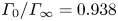$\varGamma _0/\varGamma _\infty = 0.938$, $\alpha = 0.86$, $\beta = 1.70$, $La = 15.1$.

4.5. Comparison with surfactant spreading and marginal regeneration

The behaviour of our system is reminiscent of the fingering behaviour associated with the deposition of a surfactant droplet onto a thin liquid film (Warner, Craster & Matar Reference Warner, Craster and Matar2004). We shall refer to their study as WCM henceforth. In the WCM system, a droplet of soluble surfactant is deposited on an initially surfactant free thin liquid film. The deposited droplet spreads and the surfactant advances from the droplet to surfactant-poor regions on the thin liquid film, driven by Marangoni stresses. As the leading front spreads radially outward, a severely thinned region of the film is formed between the deposited drop and the leading front. This thin region is effectively pinning the droplet in place and delaying the mass transport. Experimental observations show that this flow process is susceptible to ambient disturbances, and fingering patterns can be observed forming in the pinning region, where the film is at its thinnest (see figure 1 in WCM). The base state for the WCM system is the streamwise spreading process and the effect of disturbance in the transverse direction is studied. Their linear stability analysis reveals that, for a given set of parameters, there is a maximally amplified intermediate wavenumber associated with the transverse disturbance. This disturbance is trapped in the pinning region, rather than at the advancing front. The physical mechanism behind the growth of the disturbance can be summarized as follows: a small fluctuation in film thickness leads to a local increase in film thickness and subsequently the local surface velocity, which scales with film thickness. The increase in local surface velocity leads to enhanced advection of surfactant away from this thick film region, thereby increasing the surface tension locally. Marangoni stress draws more liquid into this locally thick, high surface tension region, contributing to the growth of the disturbance.

The instability in this study shares many common features with the surfactant spreading system. In both systems, the disturbances are amplified in the region where the liquid film is at its minimum thickness, i.e. the pinning region that restricts flow. Disturbances act to locally thicken the surfactant film (figure 7a in WCM and figure 10a). Simultaneously, the surface adsorbed surfactant concentration is depleted in the thinning region and enriched just beyond the rim (figure 7b in WCM and figure 10d). The perturbation in the surfactant concentration leads to Marangoni flows in the transverse direction that further act to increase the thickness in the already thickened film. Both systems exhibit mode selection behaviour (figure 6 in WCM and figure 8), with an intermediate wavenumber that gives the fastest growth rate. Jensen & Naire (Reference Jensen and Naire2006) conducted an extension study on the WCM system and found that self-similar structures can be determined in different regions of the spreading event by appropriately rescaling the film thickness profiles and the concentration profiles. By using the scales provided in (Jensen & Naire Reference Jensen and Naire2006), we found self-similar features in the base state solution (insets in figure 11a,b). More importantly, Jensen & Naire (Reference Jensen and Naire2006) found that, for the WCM system, the wavelength of most dangerous linearized disturbance is comparable to the width of the pinning region. This relationship confirms our observation of $m \sim R/\Delta R$.

These two systems also have features that are unique. The dominant flow driving forces are different in the two studies: the initially deposited surfactant droplet creates the surface tension gradient that drives the spreading event in the WCM study, whereas in our system, external forcing creates the surfactant gradient through advection, yielding a high surface tension region over the apex of the bubble and a low surface tension region in the bulk. Thus, the surface tension gradient in the streamwise direction for the two systems are reversed. In our system, after $t_{stop}$, the radial pressure gradient overwhelms Marangoni flow and acts to expel the liquid from the dimple (figure 11d), leading to the sustained decrease in maximum film thickness observed in figure 2(a) and figure 5 of Frostad et al. (Reference Frostad, Tammaro, Santollani, de Araujo and Fuller2016). The geometry of the substrates affects the formulation of the lubrication theory: in the WCM study the lower surface is a flat wall with a no-slip boundary condition; in this study the lower surface is an air bubble whose interfacial tension is dependent on the soluble surfactant adsorption kinetics. Finally, the curvature of the substrates affect the subsequent flow development. In the WCM study the deposited surfactant droplet expands indefinitely into domains that are covered by a clean liquid film of constant thickness. As a result, the fingers obtain significant growth (figure 14 in WCM). In contrast, in this study the curvature of the air bubble creates a domain with drastic film thickness increase beyond the rim in the radial direction (figure 10a). When perturbation disturbs the film thickness, the liquid in the dimple flows through the path of least resistance and discharges into the bulk region. In other words, the curvature of the lower surface limits the spatial domain over which disturbances can grow and, as a result, no pronounced fingering effects are observed in this study.

Finally, some discussion is in order to compare this study to the marginal regeneration phenomenon. Figure 1 of Miguet et al. (Reference Miguet, Pasquet, Rouyer, Fang and Rio2021) shows a typical marginal regeneration process developed over a freely suspended air bubble in a surfactant solution. The thin liquid film and the bulk of the surfactant solution is separated by a rim with minimum film thickness (see figure 6 of Lhuissier & Villermaux Reference Lhuissier and Villermaux2012). Thin patches of film form along this rim of pinched film. These thin patches move away from the border and displace the thicker film at the top of the bubble. These highly nonlinear, convective plumes drive the drainage over the bubble and enhance mixing inside the thin liquid film. In § 2.2 of Lhuissier & Villermaux (Reference Lhuissier and Villermaux2012) the authors conducted an extensive study of film drainage over a freely suspended air bubble and found that the wavelength of the convection cells scales with bubble size and film thickness, and evolves in time (see figures 11 and 12(b) of Lhuissier & Villermaux Reference Lhuissier and Villermaux2012).

At first glance, the characteristic rising plumes in the marginal regeneration process is not present in our system. However, if one were to define marginal regeneration as a process that is initiated with film thickness fluctuations along the rim of the film (i.e. the location of the minimum film thickness) and thinner liquid moves from the rim into the thin film region, thereby displacing the thicker film in the film region into the bulk region, then the film evolution described in this study is a type of marginal regeneration. Gros et al. (Reference Gros, Bussonnière, Nath and Cantat2021) studied marginal regeneration in horizontal surfactant films that suppress the effects of gravity. Figure 2(d) in the Gros system depicts the evolution of the film thickness profile, where film thickness fluctuations form near the meniscus and patches of thin film grow and coalesce. Despite the lack of the characteristic rising plumes, the authors found good agreement between their system and systems where the rising plumes are present. The onset of the instability described in the Gros study is similar to the present study. Furthermore, in our system, the wavenumber associated with the most dangerous mode in the linear stability analysis is different from the wavenumber of the film ridges during the stage where the dimple rapidly discharges (figure 2(b)5 versus figure 2(b)6–9). This difference suggests the presence of nonlinear effects that drive the development of the non-axisymmetric plumes observed in our system.