


1. Introduction
Thin film flows play a crucial role in many practical applications. Tear films are optical surfaces that give clarity to our vision (Braun Reference Braun2012). Spin coating is commonly used to apply photoresist coatings in photolithography (Lawrence Reference Lawrence1988). The formation and collapse of beer foams greatly dictate how consumers perceive the quality of a beer (Evans & Sheehan Reference Evans and Sheehan2002). The dynamics and stability of these films affect the evolution of their thickness and lifetime (Oron, Davis & Bankoff Reference Oron, Davis and Bankoff1997; Craster & Matar Reference Craster and Matar2009; Karakashev & Manev Reference Karakashev and Manev2015). The development of flow instabilities in these systems often triggers undesirable results in these same applications. It follows that a fundamental understanding of the stability conditions can be very helpful in schemes designed to suppress these instabilities.
Numerous factors contribute to the complexity of thin film flows and their stability. The composition of the liquid film determines the physical forces that affect fluid flows and thus their stability. Protein adsorption onto an water–air interface creates a viscoelastic interface that ensures axisymmetric film drainage, whereas surfactant-laden interfaces can exhibit non-axisymmetric drainage (Kannan, Shieh & Fuller Reference Kannan, Shieh and Fuller2019). The presence of mass transport across phases can also lead to a remarkable thin film dynamics. The well-known tears of wine phenomenon results from the preferential evaporation of ethanol, leading to the formation of a water-rich front that pulls liquid upward along the wine glass; gravity then works to pull down the accumulated liquid, forming the wine tears (Fournier & Cazabat Reference Fournier and Cazabat1992; Venerus & Simavilla Reference Venerus and Simavilla2015). Sustained mass transport across curved permeable liquid/liquid or liquid/air interfaces can trigger so-called spontaneous cyclic dimpling (Velev, Gurkov & Borwankar Reference Velev, Gurkov and Borwankar1993; Shi, Fuller & Shaqfeh Reference Shi, Fuller and Shaqfeh2020). Geometry of the substrates that support a thin film can dictate the types of instabilities that are present in a thin film system. A climbing, evaporating film on a flat, inclined, solid surface can give rise to ridge structures (Hosoi & Bush Reference Hosoi and Bush2001); silicone oil films coated on the inside of horizontally placed cylinders exhibit Rayleigh–Taylor instabilities (Balestra et al. Reference Balestra, Kofman, Brun, Scheid and Gallaire2017); and a viscous, spreading film over a spherical solid surface can yield fingering instabilities along the contact line (Takagi & Huppert Reference Takagi and Huppert2010).
Thin films over curved surfaces have been studied as model systems due to their widespread presence in a wide range of applications. Flow instabilities associated with these curved thin films have long been observed experimentally. Burrill & Woods (Reference Burrill and Woods1973) examined the drainage process of aqueous films of sodium lauryl sulphate surfactant with potassium chloride, sandwiched between a bulk oil phase and an oil droplet. The authors reported that the film undergoes a series of stages: upon the approach of the oil droplet to the bulk aqueous solution/oil interface, a dimple forms, followed by axisymmetric film drainage. In cases where the surfactant concentration is low, the axisymmetric drainage step is followed by non-axisymmetric drainage that occurs prior to film rupture. The authors attributed the non-axisymmetric drainage to a local imbalance between the shear stress and surface tension gradients. Joye, Hirasaki & Miller (Reference Joye, Hirasaki and Miller1994) studied asymmetric drainage of aqueous surfactant films in a Scheludko cell. They showed a typical drainage interferogram with an ellipsoidal pattern: the film thickens and discharges along the major axis of the ellipsoid, and the film thins and draws in liquid along the minor axis. Experimentally, they found that asymmetric drainage is associated with solutions characterized by low surface shear viscosity, whereas films with high surface shear viscosity retain axisymmetry during drainage. In their complimentary normal mode linear stability analysis, the authors found that the instability is driven by surface tension forces and, moreover, surface viscosity, elasticity and diffusivity stabilize the film. Contemporaneously, Velev et al. (Reference Velev, Constantinides, Avraam, Payatakes and Borwankar1995) demonstrated that the size of the Scheludko cell affects the manner of film drainage: films formed on a 3 mm diameter ring are generally thicker and allow for the development of asymmetric patterns similar to those reported by Burrill & Woods (Reference Burrill and Woods1973) whereas films of the same composition formed on a 0.3 mm diameter ring exhibit an axisymmetric dynamics. Even more complicated symmetry breaking patterns are observed in experiments where two droplets are forced toward each other. Figure 24 in the review written by Chan, Klaseboer & Manica (Reference Chan, Klaseboer and Manica2011) shows a high degree of symmetry breaking of a silicone oil film sandwiched between glycerol–water droplets. More recently, Zdravkov, Peters & Meijer (Reference Zdravkov, Peters and Meijer2006) reported symmetry breaking associated with diffusive polymeric thin film systems.
Although the interference patterns are fascinating to examine, the complexity of these experimental systems makes it challenging to determine the factors that contribute to the formation of the non-axisymmetric flows. Liquid composition variations and freely deformable interfaces are the primary factors that make these stability problems challenging. To address the former challenge, assumptions are often made about the distribution of the surface species and their effect on the surface velocity (Joye et al. Reference Joye, Hirasaki and Miller1994). The latter challenge is often treated by assuming a plane parallel geometry (Gumerman & Homsy Reference Gumerman and Homsy1975; Baldessari, Homsy & Leal Reference Baldessari, Homsy and Leal2007). Kaur & Leal (Reference Kaur and Leal2009) presented an approach that addressed these two challenges in a study of the stability of the liquid film sandwiched between two approaching droplets in a biaxial extensional flow. The authors first solved the time-dependent axisymmetric droplet shapes as the drops approached each other; the shapes were then used as the base state in the subsequent normal mode analysis. In other cases, the complexity of the flow requires a non-modal analysis. Balestra et al. (Reference Balestra, Badaoui, Ducimetière and Gallaire2019) investigated the fingering instability associated with a Newtonian film spreading on a horizontally placed cylinder. The gravity-driven base flow was assumed to be evolving in time and in the azimuthal direction. In the subsequent linear stability analysis, the authors introduced normal mode expansion in the axial direction of the perturbations, without constraining the time rate of the disturbance growth. With this approach, the authors were able to obtain the optimal spanwise wavenumber for the optimal gain.
Our present work provides an in-depth analysis of the instability observed by Rodríguez-Hakim et al. (Reference Rodríguez-Hakim, Barakat, Shi, Shaqfeh and Fuller2019) (see figure 5(f) in the supporting information). In our previous work, we used a combination of interferometric techniques and lubrication theory to study the evolution of an axisymmetric, evaporating, binary silicone oil film over a glass dome. Silicone oil films are shown to have a negative disjoining pressure over a glass surface. The stabilization due to this disjoining pressure allowed us to study the long-time dynamics of these films across a range of film thickness from microns to nanometres. While aqueous films have more relevance to biological applications, they readily dewet the glass surface and therefore are not suitable for studying the long-time dynamics. The inert and non-toxic nature of silicone oils also allows them to be model experimental materials, especially as a model system for lubricant oils. Furthermore, silicone oils are readily available in a wide range of surface tension and volatility, both of which play an important role in inducing Marangoni flows. In the present study, the liquid phase is composed of a low surface tension silicone oil that is highly volatile and a small fraction of a high surface tension, non-volatile silicone oil (for a 1 cSt and 5 cSt silicone oil blend  $\phi _{5\ \textrm {cSt}} \leqslant 0.3\ \textrm {vol}\%$). The dome geometry is studied for its relevance to thin film coating processes and tear film drainage (Rabiah, Scales & Fuller Reference Rabiah, Scales and Fuller2019). A well-defined substrate geometry also allows us to accurately track and quantify mass accumulation and flux, through the measurement of the film thickness. Despite the simplicity in composition and geometry, these thin films exhibited complex dynamic behaviour that arises from the competing effects of capillary pressure, Marangoni regeneration and van der Waals interactions. A thin film is generated by pushing the glass dome through an initially flat oil/air interface (figure 1). Thereafter, the dome is held fixed and the thin film evolves. When the initial solute concentration is in the so-called ‘capillary regime’, capillarity and Marangoni regeneration balance each other, leading to sustained, axisymmetric film thickening. The present study extends the previous work and examines the non-axisymmetric flows associated with binary films at a higher solute concentration (for a 1 cSt and 5 cSt silicone oil blend
  $\phi _{5\ \textrm {cSt}} \geqslant 0.35\ \textrm {vol}\%$).

Figure 1. Schematic of a glass sphere approaching a silicone oil and air interface.
The article is organized as follows. We first introduce the experimental set-up, the formulation of the lubrication theory and the numerical methods. We then describe the instability observed as the film thickens, from both an experimental and a computational perspective. In the subsequent sections, we provide a more detailed description of the flow characteristics of the observed instability, followed by a parametric study in concentration and diffusivity (the Peclet number). We finish with a generalized linear stability analysis to elucidate the mechanism behind the instability.
2. Experiment
Experiments are conducted using the custom-built dynamic fluid-film interferometer. These experiments use the same equipment set-up and procedures as presented in our previous work (Rodríguez-Hakim et al. Reference Rodríguez-Hakim, Barakat, Shi, Shaqfeh and Fuller2019). We therefore only provide a brief description in the present manuscript.
A spherical glass dome with a radius of  $a = 7.6$ mm is initially submerged in a chamber of binary silicone oil, where the binary oil is composed of a majority 1 cSt silicone oil (ShinEtsu DM-Fluid) and a dilute fraction of 5 cSt silicone oil (Clearco PSF). The relevant material properties can be found in table 1 in our previous work (Rodríguez-Hakim et al. Reference Rodríguez-Hakim, Barakat, Shi, Shaqfeh and Fuller2019). In order to examine the effects of initial solute concentration on the evolution of the film, experiments were conducted at four different initial concentrations of the 5 cSt silicone oil:
  $\phi _0 = 0.0035$, 0.005, 0.01 and
  $0.02$.
For a typical experiment, the initial distance between the apex of the glass dome and the silicone oil/air interface is  $b = 0.3$ mm. At time
  $t = 0$, a motor moves the chamber of liquid downward at a speed of
  $U = 0.05\ \textrm {mm}\ \textrm {s}^{-1}$ for a distance of
  $d = 0.35$ mm. During this period, the glass dome is held fixed and penetrates the top air/oil interface, forming a thin liquid film whose interference patterns are recorded by a top camera. Thereafter, the relative positions of the glass dome and the chamber are held fixed. Throughout this process, the chamber is open to the air and the 1 cSt silicone oil evaporates at a rate of approximately
  $E = 0.13\ \mathrm {\mu }\mathrm {m}\ \textrm {s}^{-1}$, leaving the liquid in the chamber enriched in the 5 cSt silicone oil. The evolution of the liquid film thickness is then deduced from the interference patterns. Details of the dynamical evolution of the film thickness are discussed in the results and discussion sections.
3. Theoretical model
3.1. Lubrication equations
We briefly summarize the theoretical framework that describes the dynamics of the experiments and the major physical factors that affect the non-axisymmetric thin film flow. This model expands upon our previous publication by including azimuthal flow (see Rodríguez-Hakim et al. Reference Rodríguez-Hakim, Barakat, Shi, Shaqfeh and Fuller2019). In this manuscript, the asterisk superscript represents dimensional quantities.
Initially, a solid sphere of radius  $a$ is submerged in a binary mixture of 1 cSt and 5 cSt silicone oils (figure 1). The origin is placed at the intersection of the initially flat oil/air interface and the vertical axis of the sphere. A cylindrical coordinate system (
 $z^*, r^*, \theta$) is adopted to account for the motion and the geometry of the sphere, where
  $z^*$ represents the vertical axis,
  $r^*$ represents the radial coordinate and
  $\theta$ is the azimuthal angle. At
  $t^* = 0$, the apex of the sphere is placed a distance
  $b$ below the origin. The sphere is then raised upward against gravity for a distance
  $d$, until the apex of the sphere penetrates the origin (i.e.
  $d > b$). The sphere is subsequently held fixed, mimicking the motion of the motor in the experimental apparatus. Throughout this process, the volatile 1 cSt silicone oil freely evaporates into the ambient environment. The experiments are done on a time scale over which the 1 cSt silicone oil is not significantly depleted from the bulk region (i.e. the far field). Thus, it is assumed that far from the origin, the concentration of the solute (5 cSt silicone oil) remains at its initial concentration of
  $\phi _0$. The position of the no slip glass dome is known at all times during the process and its distance to the top oil/air interface will be denoted as the film thickness,
  $h^*$. In order to describe the non-axisymmetric flows observed in the experiments, the theoretical model includes the coupled evolution of the top oil/air interface
  $h_1^*$ and the solute species concentration
  $\phi ^*$.
In developing the lubrication equations, we assume that the liquid mixture viscosity  $\mu$ and density
  $\rho$ are nearly those of the solvent, i.e. the 1 cSt silicone oil (
 $\mu = 0.82\ \mathrm {g}\ \textrm {m}^{-1}\ \textrm {s}^{-1}$ and
  $\rho = 818\ \mathrm {kg}\ \textrm {m}^{-3}$). The surface tension of the air/liquid interface is assumed to be linearly dependent on the composition
 \begin{equation} \gamma^* = \gamma_{1\ \textrm{cSt}} (1 - \phi^*) + \gamma_{5\ \textrm{cSt}} \phi^* = \gamma_{1\ \textrm{cSt}} + (\gamma_{5\ \textrm{cSt}} - \gamma_{1\ \textrm{cSt}})\phi^* , \end{equation}
where  $\gamma _{1\ \textrm {cSt}} = 16.9\ \textrm {mN}\ \textrm {m}^{-1}$ and
  $\gamma _{5\ \textrm {cSt}} = 19.7\ \textrm {mN}\ \textrm {m}^{-1}$. These assumptions are reasonable because of the dilute nature of the initial binary mixture. The evaporation rate
  $E$ of the 1 cSt silicone oil is experimentally determined by measuring evaporative mass loss under conditions similar to those in the interferometric experiments (
 $E = 0.13\ \mathrm {\mu }\mathrm {m}\ \textrm {s}^{-1}$). Evaporation induced thermal effects are neglected. In our previous work, thermal imaging of the evaporating thin film showed negligible thermocapillary effects (Rodríguez-Hakim et al. Reference Rodríguez-Hakim, Barakat, Shi, Shaqfeh and Fuller2019). Over the range of concentrations studied in this work, the film never thins to nanoscopic values and the van der Waals interactions have a negligible effect on the dynamics of the film. However, to be consistent with our previous model formulation, the Hamaker constant
  $A$ is assumed to be
  $10^{-18}$ J. The binary diffusivity
  $D = 0.0019\ \mathrm {mm}^{2}\ \mathrm {s}^{-1}$ is extrapolated from the diffusivity of 1 cSt silicone oil in high viscosity silicone oils (1000–100 000 cSt), following the procedures described by Walls, Meiburg & Fuller (Reference Walls, Meiburg and Fuller2018). Due to the wide range of extrapolation, there is high uncertainty associated with this extrapolated value. Thus, in the calculations described below, we will examine a range of Péclet number and, specifically, the effect of Péclet number on the film stability is examined in § 4.3.
To produce a set of non-dimensionalized equations, the following scales are chosen. The obvious scale for solute concentration is its initial concentration  $\phi _0$. The axial length scale is the captured film thickness at the time when the motor stops moving:
  $a\sqrt {Ca}$, where the capillary number
  $Ca \equiv {\mu U}/{\gamma _{1\ \textrm {cSt}}}$. It follows from continuity that the radial and azimuthal length scales are
  $a Ca^{1/4}$. The pressure scale
  $\gamma _{1\ \textrm {cSt}}/a$ is obtained by balancing capillary stresses with the pressure. Finally, the axial velocity scale is
  $U$. The dimensionless quantities are thus defined as (Rodríguez-Hakim et al. Reference Rodríguez-Hakim, Barakat, Shi, Shaqfeh and Fuller2019)
 \begin{align} r = \frac{r}{a Ca^{1/4}}{,}\quad t = \frac{\gamma_{1\ \textrm{cSt}} Ca^{1/2}}{\mu a} t^*{,} \quad \phi = \frac{\phi^*}{\phi_0}{,}\quad h = \frac{h^*}{a Ca^{1/2}},\quad \textrm{and}\quad P = \frac{aP^*}{\gamma_{1\ \textrm{cSt}}}. \end{align}
 After applying the above scales, the dimensionless governing equations for the film thickness  $h(t,r,\theta )$ and the solute concentration
  $\phi (t, r, \theta )$ are
 \begin{align} &\frac{\partial {h}}{\partial {t}}+ \frac{1}{r}\frac{\partial}{\partial r}\left(rh\left\langle {v_r} \right\rangle\right) + \frac{1}{r}\frac{\partial {}}{\partial {\theta}} \left( h\left\langle {v_\theta} \right\rangle \right)={-} Ev(1 - \phi_0 \phi), \end{align}
 \begin{align} &\frac{\partial {\phi}}{\partial {t}} +\left( { \left\langle {v_r} \right\rangle - \frac{1}{Pe} \frac{1}{h} \frac{\partial {h}}{\partial {r}} } \right) \frac{\partial {\phi}}{\partial {r}} +\left( { \left\langle {v_\theta} \right\rangle - \frac{1}{Pe}\frac{1}{h}\frac{1}{r}\frac{\partial h}{\partial \theta} } \right) \frac{1}{r}\frac{\partial \phi}{\partial \theta} \nonumber\\ &\quad -\frac{1}{Pe} \left( { \frac{1}{r}\frac{\partial}{\partial r}\left(r\frac{\partial {\phi} }{\partial r}\right) + \frac{1}{r^2}\frac{\partial^2 \phi}{\partial \theta^2} } \right) =\frac{Ev}{h}\phi(1-\phi_0\phi), \end{align}
 \begin{align} &P = 2 -\frac{1}{r}\frac{\partial}{\partial r}\left(r\frac{\partial {h} }{\partial r}\right) - \frac{1}{r^2}\frac{\partial^2 h}{\partial \theta^2} + Bo (h - h_\infty) - \frac{Ha}{h^3}, \end{align}
where
 \begin{equation} \left\langle {v_r} \right\rangle ={-}\frac{h^2}{3} \frac{\partial {P}}{\partial {r}}+ \frac{Ma}{2} h \frac{\partial {\phi}}{\partial {r}}, \end{equation}
and
 \begin{equation} \left\langle {v_\theta} \right\rangle ={-}\frac{h^2}{3}\frac{1}{r}\frac{\partial P}{\partial \theta} + \frac{Ma}{2} h \frac{1}{r}\frac{\partial \phi}{\partial \theta}. \end{equation}
The corresponding initial and boundary conditions are
 \begin{equation} \left.\begin{gathered} \text{at } t = 0: h = h_\infty,\ \phi = 1,\ P = 0, \\ \text{as } r\rightarrow \infty: h \rightarrow h_\infty,\ \phi \rightarrow 1,\ P \rightarrow 0, \\ \text{and } \psi(\theta) = \psi(\theta + 2{\rm \pi}) \text{, where } \psi = h, \phi, P. \end{gathered}\right\} \end{equation}
The far-field film thickness is defined as
 \begin{equation} h_\infty (t,r) = \begin{cases} \dfrac{b}{a\sqrt{Ca}} + \dfrac{r^2}{2} - Ev (1 - \phi_0) t - t & \left(t < t_{stop}\equiv \dfrac{d}{a\sqrt{Ca}}\right) \\ \dfrac{b}{a\sqrt{Ca}} + \dfrac{r^2}{2} - Ev (1 - \phi_0) t - t_{stop} & (t\geqslant t_{stop}). \end{cases} \end{equation}
 Finally, to complete the model, we shall briefly discuss the dimensionless parameters. The capillary number  $Ca = {\mu U}/{\gamma _{1\ \textrm {cSt}}}$ compares the viscous stresses to capillary stresses. The Bond number
  $Bo = {\rho g a^2 \sqrt {Ca}}/{\gamma _{1\ \textrm {cSt}}}$ is defined as the square of the ratio of the capillary length scale and the characteristic length scale (
 $g$ is the gravitational acceleration:
  $g = 9.8\ \textrm {m}\ \textrm {s}^{-2}$). The Hamaker number
  $Ha = {A}/{6 {\rm \pi}a^2 Ca^{3/2}\gamma _{1\ \textrm {cSt}}}$ gives an indication of the strength of the van der Waals interactions to the capillary forces. The Marangoni number
  $Ma = ({\phi _0 (\gamma _{5\ \textrm {cSt}} - \gamma _{1 \ \textrm {cSt}})\sqrt {Ca}})/{\mu U}$ compares the solutocapillary stresses to the viscous stresses. The evaporation number
  $Ev = {E}/{U}$ is the ratio of the evaporation rate to the characteristic velocity scale in the axial direction. Finally, the Péclet number
  ${a U}/{D}$ compares the length scales of advection and diffusion. We focus on only one silicone oil blend: 1 cSt as the solvent and 5 cSt as the solute, one glass dome and one motor speed. Therefore, the aforementioned dimensionless parameters remain constant for the system of interest and only
  $\phi _0$ will be varied. From the extrapolated diffusivity, the corresponding Péclet number is
  $Pe = 200$. However, because of the inaccuracy associated with the power-law-based extrapolation for the diffusivity, we examine two additional Péclet numbers that are spaced on a log scale around the estimated Péclet number:
  $Pe = 100$ and
  $Pe = 1000$. Table 1 provides a summary of the parameter definitions and their values used in this study.
Table 1. Dimensionless parameters used in this study.

3.2. Numerical methods
The governing equations are spatially discretized using the finite-difference method. To avoid the singular point in the cylindrical coordinate system at  $r = 0$, the two-dimensional mesh is generated following the suggestions made by Mohseni & Colonius (Reference Mohseni and Colonius2000). A radially stretched map is used such that 62 % of the grid points are smoothly clustered over
  $r \in [0,1]$ and the remaining 38 % of the points are positioned over
  $r \in (1, R_{max}]$, where
  $R_{max}$ represents the size of the simulation domain in the radial direction. A Crank–Nicolson scheme with adaptive time stepping is employed for the time advancement (Rodríguez-Hakim et al. Reference Rodríguez-Hakim, Barakat, Shi, Shaqfeh and Fuller2019). At each iteration, the linearized equations are solved using the generalized minimal residual method (GMRES) solver provided in the PETSc package (Balay et al. Reference Balay2019). Verification against the one-dimensional solution and validation against experimental data are presented in the following section.
4. Results and discussion
4.1. Symmetry breaking
In this section, we describe symmetry breaking associated with the dynamics of an evaporating binary liquid film over a spherical glass dome. Expanding on our previous study (Rodríguez-Hakim et al. Reference Rodríguez-Hakim, Barakat, Shi, Shaqfeh and Fuller2019), the present work is focused on binary blends of 1 cSt and 5 cSt silicone oils at a higher volume fraction of the non-volatile, high surface tension species (5 cSt,  $\phi _0 \geqslant 0.0035$). Similar to the thin film dynamics that we previously described as being in the ‘capillary regime’ (1 cSt and 5 cSt blend,
  $0.0002 \lesssim \phi _0 \leqslant 0.003$), the film dynamics for higher concentrations of the non-volatile species demonstrates initial drainage due to the squeezing motion of the glass dome. A concentration gradient is simultaneously developed as the volatile species evaporates. This concentration gradient drives a Marangoni flow toward the apex of the glass dome, forming a solute-rich mound, bounded by the rim,
  $R(t,\theta )$, where the film thickness is at its minimum. Because the solute-enriched mound region is characterized by a higher surface tension than that in the bulk surrounding region, the liquid is continuously drawn into the mound. In the previously described capillary regime, the mound volume continues to grow in an axisymmetric manner throughout this process. However, at higher initial non-volatile solute concentration,
  $\phi _0$, while the mound volume is growing, the film thickness at the rim of the mound grows unevenly, leading to symmetry breaking and non-axisymmetric liquid discharge from the mound into the bulk.
Figure 2 contains interferograms and their corresponding film thickness maps, before, during and after a mound discharge event for a 1.00–5.00 cSt ( $\phi _0 = 0.005$) blend. Figure 3 provides the parameter matched simulation film thickness and solute concentration surfaces at the corresponding time points. At the start of visible symmetry breaking, the film thickness and solute concentration fields remain near axisymmetric (figures 2d and 3a,d). As the disturbances grow, one side of the film thins while its opposite side thickens (figures 2e and 3b), leading to a visible loss of axisymmetry. As the asymmetry becomes even more apparent, the apex of the mound shifts away from
  $r = 0$ and toward the direction of film thickening. Simultaneously, the solute-rich region is convected toward the region of film thickening (figure 3e). The spatial shift in the high surface tension region leads to an azimuthal Marangoni flow that pulls more liquid toward the location of the radially shifted mound. Eventually, the region of increased film thickness grows to such an extent that the previously well-defined rim becomes a shoulder and there is no clear distinction between the mound region and the thicker, bulk region in the direction of film thickening (figures 2f and 3c). This process completes one cycle of mound discharge.

Figure 2. Interference patterns (a–c,  $t = 165$,
  $t = 218$,
  $t = 236$) and the corresponding experimental dimensionless film thickness profiles (d–f) during a mound discharge event for a binary mixture of 1 cSt silicone oil with 0.5 vol% of 5 cSt silicone oil. The diameter of the interferograms corresponds to 1 mm and the horizontal bars in the film thickness profiles indicate a dimensionless radial length scale of 1.

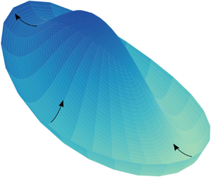
Figure 3. Film thickness and concentration profiles during a mound discharge event of a simulation conducted at  $\phi _0 = 0.005$ and
  $Pe = 200$. The other simulation parameters are
  $Ca = 2.426 \times 10^{-6}$,
  $Bo = 0.0427$,
  $Ma/\phi _0 = 106.4$,
  $Ev = 0.0026$,
  $t_{stop} = 29.57$ and
  $Ha = 1.438\times 10^{-5}$. For the rest of the paper, these parameters are kept constant. (a–c) Film thickness surface plots at time points 356, 369 and 381. The horizontal bar indicates a dimensionless radial length scale of 1. (d–f) Contour plots of the non-evaporative species concentration (in filled colour) overlaid with the location of the rim (white lines). The directions of mound discharge (‘Ds’), film thinning (‘Th’) and the locations between the two points (‘
 $\textrm {Ds} + {\rm \pi}/2$’ and ‘
 $\textrm {Th} + {\rm \pi}/2$’) are labelled with white dots. The arrows plotted over the four positions indicate the general flow direction at that point. The length of the arrows gives a general indication of the growth in flow magnitude. The arrow lengths are not drawn to scale.
In the experiments, ambient disturbance events such as ambient air disturbances and vibrations can induce a mound discharge event; in the numerical simulation shown in figure 3, the accumulated numerical error leads to the eventual mound discharge event. Despite the difference in the source of the disturbance, the simulation and the experiment agree quantitatively in the form of the break in symmetry, suggesting that the most dangerous mode follows the form of the observed disturbance in the simulations.
Based on the observations above, we conducted an analysis of the evolution of the rim thickness and the apex location to further characterize the mound discharge event and compare the simulation against the experiment. The rim film thickness ( $h_R$) corresponding to the panels shown in figures 2 and 3 is extracted and plotted in figures 4(a) and 4(d). When plotted against the azimuthal angle, the rim film thickness takes the approximate form of a cosine function. Fourier transform of
  $h_R$ confirms this observation (figure 4b,e): as the mound discharges, the amplitude of the signal with an azimuthal wavenumber of one grows (
 $m = 1$, vertical dashed line). Thus, for this system, apparently the disturbance that is amplified follows the form of
  $\tilde {\psi }(t,r,\theta ) = \cos (\theta ) \hat {\psi }(t,r)$, where
  $\psi = h_1, \phi$. During the discharge, the apex of the mound moves away from
  $r = 0$ at an exponential rate (figure 4c,f). In the simulation, during
  $0 < t < 310$, the flat line in the radial position of the apex signifies the smallest radial grid point away from
  $r = 0$ (for details on meshing, see the numerical methods section).

Figure 4. Comparison of selected quantities associated with experimental data (a–c) presented in figure 2 and the parameter matched simulation (d–f) results presented in figure 3. (a,d) Rim film thickness before, during and after mound discharge. (b,e) Fourier transform of the rim film thickness presented in (a,d). The vertical dashed line is plotted over the azimuthal wavenumber  $m = 1$ to guide the eye. (c,f) Radial position of the apex of the mound as a function of time.
4.2. Flow characteristics during symmetry breaking
In this section, we examine flow characteristics during the symmetry breaking event by comparing the results of two-dimensional and one-dimensional (1-D) (i.e. axisymmetric) simulations conducted with the same set of parameters (i.e. those presented in figure 3). The most visible indication of a mound discharge event is the deviation in the mound volume ( $V_m$ defined below) in the 2-D simulation as compared to the 1-D simulation. In the 1-D simulation, the assumption of axisymmetry restricts the solution of the governing equations to be only a function of
  $t$ and
  $r$. Therefore, the solution does not have a second spatial dimension into which momentum can be transferred. In the 2-D simulation, the liquid can move in both the radial and the azimuthal directions. Thus in these two cases, there is a distinct difference in the evolution of the ‘mound volume’, defined as
 \begin{equation} V_m(t) = \int_0^{2{\rm \pi}} \int_0^{R(t,\theta)} h(t,r,\theta) r \,\textrm{d}r \,\textrm{d}\theta, \end{equation}
where the rim position,  $R(t,\theta )$, is the radial location of the minimum film thickness in a given azimuthal direction. For the 1-D simulation, this quantity simply becomes
 \begin{equation} V_{m,1D}(t) = 2{\rm \pi} \int_0^{R(t)} h(t,r) r \,\textrm{d}r. \end{equation}
Figure 5(a) shows the comparison of the mound volume evolution of the 2-D and 1-D simulations. In both sets of simulations, the mound volume first undergoes a transient growth, after which the mound enters a monotonic growth region beyond  $t = 76$. From
  $t = 76$ until approximately
  $t = 356$, the mound volume grows at the same rate for both 1-D and 2-D simulations, and there is apparently no break in symmetry. At
  $t = 368$, the disturbance in the 2-D simulation has grown to a large enough amplitude to create an asymmetric mound discharge event, thus leading to a sharp drop in the mound volume. In the 1-D simulation, the mound volume continues to grow.

Figure 5. Comparison of the time evolutions of selected quantities associated with the simulation shown in figure 3 and the corresponding 1-D axisymmetric simulation. (a) Mound volume evolution. (b) Apex and rim film thickness. In the 1-D simulation, the apex is located at  $r = 0$ and the rim is located at the position of minimum film thickness. For the 2-D simulation, the film thicknesses at the apex and at the rim on the opposing sides along the direction of the mound discharge are plotted; ‘Ds’ and ‘Th’ stand for ‘discharging side’ and ‘thinning side’ respectively. (c) Radial velocity at the rim locations. (d) Pressure (‘
 $P$’) and Marangoni (‘
 $M$’) contributions to the radial velocity at the rim locations. (e) Azimuthal velocities at the rim locations that are
  ${\rm \pi}$/2 offset from the discharging and thinning sides. (f) Pressure and Marangoni contributions to the azimuthal velocity at the rim locations presented in (e).
A second set of measures that indicate symmetry breaking are the film thicknesses at both the apex and the rim. In a 2-D simulation, the apex is defined as the location of the maximum film thickness within the mound region; whereas in a 1-D simulation, the apex is always located at  $r = 0$ (figure 5b). Similar to the mound volume evolution, the apex film thickness in the 2-D simulation decreases at around
  $t = 368$ (i.e. at the onset of a discharge event), while its 1-D counterpart grows indefinitely due to the symmetry constraint. For the 2-D simulation, the locations of the maximum and minimum rim film thickness can be examined. These opposing rim locations are of interest because they are positioned along the axis of mound discharge, and thus where film thickness changes are most rapid and pronounced. The direction in which the film thickens during discharge is referred to as the discharging side (‘Ds’). This is the side where the apex and rim will eventually merge, thus signalling the end of a mound discharge event. The opposing side is referred to as the thinning side (‘Th’), where the film thickness decreases during discharge.
To examine the total liquid flow into and out of the mound region, we look at the depth averaged radial and azimuthal volumetric flux per unit circumference evaluated at the rim
 \begin{align} \left\langle {v_r} \right\rangle_R = \left.\left( {-\frac{h^2}{3}\frac{\partial {P}}{\partial {r}} + \frac{Ma}{2}h\frac{\partial {\phi}}{\partial {r}}} \right) \right|_R,\quad \text{and}\quad \left\langle {v_\theta} \right\rangle_R = \left.\left( { -\frac{h^2}{3}\frac{1}{r}\frac{\partial P}{\partial \theta} + \frac{Ma}{2} h \frac{1}{r}\frac{\partial \phi}{\partial \theta}} \right) \right|_R. \end{align}
Both velocities have two contributing terms: the pressure contribution and the Marangoni contribution (figure 5c–f). For the pressure contribution of the radial velocity, the dominant term comes from capillary forces. Based on the definition of the coordinate system, a positive value in  $\left \langle {v_r} \right \rangle _R$ signifies liquid flow away from
  $r = 0$ towards the bulk. During the transient mound growth (
 $t_{stop} < t < 33$), the film thickness grows monotonically in all azimuthal directions. The volume of the mound is then reduced quickly as liquid flows out axisymmetrically due to the dominant pressure contributions (figure 5(d),
  $33 < t < 76$). During this period, a concentration gradient is established such that the Marangoni term overwhelms the pressure term, leading to an inward radial flux toward
  $r = 0$ (
 $\left \langle {v_r} \right \rangle _R < 0$,
  $76 < t < 178$). The film thickens as a result of Marangoni regeneration, thereby increasing the magnitude of both contributions and reducing the magnitude of the total inward flow (figure 5(c),
  $178 < t < 356$). Soon after, the difference in rim film thickness between the discharging and thinning side increases. On the discharging side, the film thickens and the pressure contribution to the radial flow eventually overwhelms the Marangoni flow, leading to the eventual outward discharge flow (figure 5(c) when the dash-dotted line goes from being negative to positive). On the thinning side, the film thickness is further reduced and both contributions to the radial flow decrease in magnitude; however, the Marangoni contribution decreases at a slower rate, leading to a stronger inward flow (in figure 5(c) the solid line grows more negative). In addition to the change in flow magnitude on the two opposing sides, as the mound is shifted in the direction of discharge, the solute rich mound gets convected. The off-centre mound creates secondary Marangoni flows in the azimuthal direction (thus a non-zero
  $\left \langle {v_\theta } \right \rangle _R$) that draws more liquid into the mound and speeds its radial discharge (figure 3d–f).
Finally, we look at the azimuthal flow  $\left \langle {v_\theta } \right \rangle _R$ at selected rim locations. Figure 5(e,f) shows the magnitude of the azimuthal flow at rim locations that are
  ${\rm \pi} /2$ away from the discharging and thinning locations. These locations were chosen because they have the maximum azimuthal flow amplitude; whereas, at the discharging and thinning locations, the magnitude of the azimuthal flow is small due to the mirror symmetry along the axis of mound discharge. The azimuthal flow has negligible magnitude until significant symmetry breaking occurs (
 $0 < t < 330$). When the mound discharges along the axis of symmetry breaking, it convects the high surface tension liquid away from the
  $z$-axis, thus rendering the concentration/surface tension profile non-axisymmetric. The disruption in the concentration profile leads to an increase in the magnitude of the azimuthal Marangoni flow, which is slightly damped by the pressure contributions (figure 5f). Overall, at
  ${\rm \pi} /2$ away from the discharging and thinning rim locations, the azimuthal flows drive fluid toward the discharging side, thus further thickening the film at that location (figure 5(f), and see the arrows in figure 3).
4.3. Effects of solute concentration and diffusivity on the onset of symmetry breaking
As one can deduce, of primary interest are the effects of  $\phi _0$ and
  $Pe$ on the onset of symmetry breaking. The experimental set-up is subjected to ambient disturbances throughout an experiment. In simulations, we can inject a known form of disturbance at a specific time point to determine its effect on the subsequent mound discharge. Because the sources and amplitudes of the disturbance in the experiments and the simulations are different, we choose to compare the trends in how the experiments and simulations respond to changes in one input parameter. To this end, we introduce the following form of disturbance at
  $t = 127$ for all the simulations shown in this section:
 \begin{equation} \tilde{h}_{1,ini} = C_h \cos(\theta) \frac{r}{2R^3 + r^3}, \quad\text{and}\quad \tilde{\phi}_{ini} = C_\phi \cos(\theta) \frac{r}{4R^5 + r^5}, \end{equation}
where  $C$ is a normalization coefficient. The analytical form of the injected disturbance was found by fitting a smooth surface to the difference between the 2-D solution during mound discharge and the corresponding solution in the 1-D simulation. Noise-injection time of
  $t = 127$ is chosen such that all simulations studied are in the Marangoni regeneration regime and have yet to break axisymmetric flow. The rim location,
  $R$, is found for each simulation at the time of the noise injection. The normalization coefficients,
  $C_h$ and
  $C_\phi$, are chosen such that the injected disturbance is sufficiently large to create a system response that is not overshadowed by the intrinsic numerical difference between the 2-D and the axisymmetric simulations, while small enough such that there is agreement with the linearized disturbance evolution at short times. We will devote more discussion to the linear stability analysis in the next section. (See Appendix A for the specific values of the normalization coefficients and a comparison of the radial profiles of the disturbance quantities.)
We study the binary mixtures at four initial concentrations ( $\phi _0 = 0.0035, 0.005, 0.01, 0.02$). These concentrations were chosen such that the onset of the discharge time in the experiments is individually distinguishable. Figure 6 shows experimental and simulation apex film thickness and mound volume evolution up to the end of the first mound discharge event. Marangoni driving forces increase in magnitude as the initial concentration increases. As a result, Marangoni regeneration happens at an earlier time and mound discharge also happens more quickly. Figure 7 shows the experimental and simulation mound discharge time plotted as a function of initial concentration. In the simulations, three Péclet numbers were examined to account for the uncertainty in diffusivity. The diffusivity that corresponds to
  $Pe = 200$ is extrapolated from four binary diffusivities of 1 cSt silicone oil at 1000, 10 000, 60 000 and 100 000 cSt, reported by Walls et al. (Reference Walls, Meiburg and Fuller2018). Clearly the extrapolation has a high level of uncertainty associated with it. Thus we examine three Péclet numbers to account for this uncertainty.

Figure 6. Time evolution of experimental (a) and simulation (b) apex film thickness at four concentrations. The error bars in the experimental data represent the standard deviation taken from fifteen experiments conducted for each concentration. The simulations were conducted at  $Pe = 200$,
  $Ca = 2.426 \times 10^{-6}$,
  $Bo = 0.0427$,
  $Ma/\phi _0 = 106.4$,
  $Ev = 0.0026$,
  $t_{stop} = 29.57$ and
  $Ha = 1.438\times 10^{-5}$. For each simulation, the same disturbance was introduced at
  $t = 127$.

Figure 7. Effects of initial concentration on experimental (a) and simulation (b) mound discharge time. For each simulation, the same disturbance was introduced at  $t = 127$. Except for
  $\phi _0$ and
  $Pe$, all other simulation parameters are the same as the ones used in figure 3.
For all three Péclet numbers, as the concentration increases, the time for the mound to discharge decreases, in agreement with the experimental observations. For the simulation conducted at  $\phi _0 = 0.0035, Pe = 100$, the disturbance ultimately decayed, indicating a stability boundary in the parameter space of
  $\phi _0$ and
  $Pe$. This strongly suggests that diffusion plays a crucial role in stabilizing the system. In the experiments, the film thickness profile remained axisymmetric for
  $\phi _0 \leqslant 0.003$ and symmetry breaking is observed for
  $\phi _0 \geqslant 0.0035$. This observation of the stability cross-over in the experiments further validates the predictions of our theoretical model. Note that no attempt has been made to examine the complete stability boundary in
  $\phi _0$ and
  $Pe$ space, and this is a fruitful direction for future studies.
In the range of concentrations and Péclet numbers studied, it is unclear if there is a critical film thickness or a critical mound volume at which the system will discharge. A closer look at the disturbance evolution is necessary to elucidate the mechanism behind this instability. In this context, we therefore turn to linear stability analysis.
4.4. Linear stability analysis
In this section, we examine the system response to an asymptotically small perturbation, by looking at the linearized disturbance evolution. Based on experimental observations, the initially axisymmetric film evolves until it transitions to a non-axisymmetric state and the Marangoni-regenerated mound discharges along a given axis. The constant presence of evaporation indicates that the system continuously evolves in time. Thus, the base state in this case is the axisymmetric, 1-D solution that evolves in time and is a function of only the radial coordinate. The complexity of the base state suggests that we formulate a linearized initial value problem to study the transient response of the system to small perturbations (Schmid Reference Schmid2007), without making the assumption of exponential disturbance growth in time (the usual eigenvalue problem). The linearized disturbance equations are derived by taking the difference in the governing equations for the 2-D and the 1-D systems, followed by neglecting all nonlinear terms in the disturbance quantities,  $\tilde {\psi } \equiv \psi _{2D} - \psi _{1D}$, where
  $\psi$ represents
  $h_1$ (position of the top air/oil interface),
  $\phi$,
  $\left \langle {v_r} \right \rangle$,
  $\left \langle {v_\theta } \right \rangle$ and
  $P$. We seek solutions in the form of
  $\tilde {\psi } = \exp (\textrm {i}m\theta )\hat {\psi }(t,r)$, i.e. the disturbance quantities in the azimuthal direction follow a sinusoidal form. After some algebra, the disturbance quantities are governed by the following set of linearized disturbance equations:
 \begin{align} &\frac{\partial {\hat{h}_1}}{\partial {t}} + \frac{1}{r}\frac{\partial}{\partial r}\left(rh_{1D}\left\langle {\hat{v}_r} \right\rangle\right) + \frac{1}{r}\frac{\partial}{\partial r}\left(r\left\langle {v_r} \right\rangle_{1D}\hat{h}_1\right) + h_{1D} \frac{\textrm{i}m}{r} \left\langle {\hat{v}_\theta} \right\rangle - Ev\phi_0 \hat{\phi} = 0, \end{align}
 \begin{align} &\frac{\partial {\hat{\phi}}}{\partial {t}} +\left\langle {v_r} \right\rangle_{1D} \frac{\partial {\hat{\phi}}}{\partial {r}} +\frac{\partial {\phi_{1D}}}{\partial {r}} \left\langle {\hat{v}_r} \right\rangle -\frac{1}{Pe}\frac{1}{r}\frac{\partial}{\partial r}\left(r\frac{\partial {\hat{\phi}} }{\partial r}\right) +\frac{1}{Pe}\frac{m^2}{r^2}\hat{\phi} +\cdots \nonumber\\ &\quad-\frac{1}{Pe} \frac{1}{h_{1D}} \frac{\partial {\phi_{1D}}}{\partial {r}} \frac{\partial {\hat{h}_1}}{\partial {r}} - \frac{1}{Pe} \frac{1}{h_{1D}} \frac{\partial {h_{1D}}}{\partial {r}} \frac{\partial {\hat{\phi}}}{\partial {r}} +\frac{1}{Pe} \frac{1}{h_{1D}^2} \frac{\partial {h_{1D}}}{\partial {r}} \frac{\partial {\phi_{1D}}}{\partial {r}} \hat{h}_1 \nonumber\\ &\qquad = Ev \frac{1 - 2\phi_0\phi_{1D}}{h_{1D}}\hat{\phi} - Ev \frac{\phi_{1D}(1 - \phi_0\phi_{1D})}{h_{1D}^2} \hat{h}_1, \end{align}
where
 \begin{gather} \left\langle {\hat{v}_r} \right\rangle ={-}\frac{h_{1D}^2}{3} \frac{\partial {\hat{P}}}{\partial {r}} -\frac{2}{3} h_{1D} \frac{\partial {P_{1D}}}{\partial {r}} \hat{h}_1 +\frac{Ma}{2}\frac{\partial {\phi_{1D}}}{\partial {r}} \hat{h}_1 +\frac{Ma}{2}h_{1D}\frac{\partial {\hat{\phi}}}{\partial {r}}, \end{gather}
 \begin{gather}\left\langle {\hat{v}_\theta} \right\rangle ={-}\frac{h_{1D}^2}{3} \frac{\textrm{i}m}{r} \hat{P} + \frac{Ma}{2} h_{1D} \frac{\textrm{i}m}{r} \hat{\phi},\quad \text{and} \end{gather}
 \begin{gather}\hat{P} ={-}\frac{1}{r}\frac{\partial}{\partial r}\left(r\frac{\partial {\hat{h}_1} }{\partial r}\right) + \frac{m^2}{r^2} \hat{h}_1 + Bo \hat{h}_1 + \frac{3Ha}{h_{1D}^4} \hat{h}_1. \end{gather}
 In the numerical implementation, the above equations are rearranged such that only  $\hat {h}_1$ and
  $\hat {\phi }$ are solved with an initial condition that captures the form, as described above (4.4a,b), of what is apparently the ‘most dangerous mode’ – i.e. a smooth approximation to the difference between the fully 2-D simulations during mound discharge and the corresponding 1-D axisymmetric state. By setting
  $m$ to an integer value and applying the following initial and boundary conditions, we complete the initial value problem
 \begin{gather} \hat{h}_1(t_{ini},r) = \frac{r}{2R^3 + r^3}, \end{gather}
 \begin{gather}\hat{\phi}(t_{ini},r) = \frac{r}{4R^5 + r^5}, \quad\text{and} \end{gather}
 \begin{gather}\text{as } r\rightarrow\infty, \quad\hat{h}_1 \rightarrow 0, \quad\frac{\partial {\hat{h}_1}}{\partial {r}} \rightarrow 0, \quad\frac{\partial {^2\hat{h}_1}}{\partial {r^2}} \rightarrow 0, \quad\frac{\partial {^3\hat{h}_1}}{\partial {r^3}} \rightarrow 0,\quad \hat{\phi} \rightarrow 0, \quad\frac{\partial {\hat{\phi}}}{\partial {r}} \rightarrow 0. \end{gather}
In the linear stability analysis, we are particularly interested in the ‘gain’ of the linearized disturbance quantities, specifically,
 \begin{equation} G(t) \equiv \frac{\displaystyle\int_0^\infty \left( {\hat{h}_1^2 + \hat{\phi}^2} \right) r \,\textrm{d}r}{ \displaystyle\int_0^\infty\left( {\hat{h}_{1,ini}^2 + \hat{\phi}_{ini}^2} \right) r \,\textrm{d}r}. \end{equation}
Correspondingly, the gain associated with the disturbances injected into the 2-D simulation is defined as
 \begin{equation} G_{2D}(t) = \frac{\displaystyle\int_0^{2{\rm \pi}} \displaystyle\int_0^\infty \left( {(h_{1,2D} - h_{1,1D})^2 + (\phi_{2D} - \phi_{1D})^2} \right) r \,\textrm{d}r \,\textrm{d}\theta} {\int_0^{2{\rm \pi}} \int_0^\infty \left( {\tilde{h}_{1,ini}^2 + \tilde{\phi}_{ini}^2} \right) r \,\textrm{d}r \,\textrm{d}\theta}. \end{equation}
Note that the gains, as defined in (4.13) and (4.14), are suitably scaled inner products of the fluctuations in  $h_1$ and
  $\phi$. When the gain of the disturbances decays to a value well below one, the system is stable, whereas a value above one indicates disturbance growth. By comparing the gain associated with the linearized disturbances,
  $G(t)$ and
  $G_{2D}$ , we can also establish the time range in which the linear stability analysis is applicable. To such an end, we examine two simulations in the
  $\phi _0 - Pe$ parameter space:
  $\phi _0 = 0.0035, Pe = 100$ and
  $\phi _0 = 0.005, Pe = 200$. In the full 2-D simulations
  $\phi _0 = 0.0035, Pe = 100$ is the only parameter set with a long-time stable response, whereas the other parameter set gives an unstable response.
Figure 8 shows the evolution of the gain of the disturbances for these two parameter sets. In the 2-D simulations, the disturbance defined by (4.4a,b) is introduced at  $t = 127$ as a one-time noise injection. The 2-D simulations are evolved and we track the deviation from the corresponding axisymmetric, 1-D simulation without noise injection. We examine the most dangerous azimuthal mode
  $m = 1$. Higher-order modes are found to be more stable (see Appendix A).

Figure 8. (a,b) Contain comparisons of mound volume evolution between the corresponding noise-injected 2-D simulations and the axisymmetric 1-D simulations. (c,d) Contain comparisons of the gain of the linearized disturbance (circles) to the gain associated with the injected disturbances in the 2-D simulations (lines). (a,c) Correspond to the simulations conducted at  $\phi _0 = 0.0035$ and
  $Pe = 100$. (b,d) Correspond to the simulations conducted at
  $\phi _0 = 0.005$ and
  $Pe = 200$. The noise is injected at
  $t = 127$.
The evolution in mound volume gives a direct visual clue to the onset of mound discharge. For the stable case ( $\phi _0 = 0.0035$,
  $Pe = 100$, figure 8a), up to
  $t = 600$, there is no significant difference between the mound volume in the 2-D simulation with noise injection and that in the axisymmetric simulation, signifying that the injected noise decays over time. For the unstable case (
 $\phi _0 = 0.005$,
  $Pe = 200$, figure 8b), the mound discharged by
  $t = 200$, shortly after the noise injection, signifying that the injected noise brings about the onset of symmetry breaking.
Figures 8(c) and 8(d) compare the disturbance gain obtained from the 2-D simulation with noise injection and from linearized disturbance equations. For the stable case, there is good agreement in the gain from the noise injection at  $t = 127$ until
  $t = 250$ (figure 8c). The amplitude of the gain first grows, reaching its peak value at
  $t = 150$. It then decays to its initial value of one at
  $t = 200$. Thereafter, the disturbance further decays, showing that the system is linearly stable for the parameter set of
  $\phi _0 = 0.0035$ and
  $Pe = 100$. In the unstable case, the disturbance gain grows immediately after noise injection (figure 8d). The linearized disturbance growth follows that of the 2-D simulation until
  $t = 190$, at which point the mound in the 2-D simulation starts to discharge. From
  $t = 190$ onward, the amplitude of the gain of the linearized disturbances grows exponentially, while the gain in the 2-D simulation is affected by secondary, nonlinear flows associated with symmetry breaking.
The linear stability analysis conducted for these two parameter sets has shown that, at  $t = 127$, one is linearly stable while the other one is linearly unstable. This analysis will now be carried out at different time points, i.e. the initial value problem will be solved at different starting points during Marangoni regeneration. For the linearly stable case (
 $\phi _0 = 0.0035$ and
  $Pe = 100$, figure 9a), the system shows a linearly stable response at
  $t_{ini} = 127$, 152, 178, 203, 229 and
  $254$. The growth rate and magnitude of the gain differ for each
  $t_{ini}$, but they all eventually decay, showing that this parameter set is indeed linearly stable. For the other parameter set, the disturbances immediately grow when the linearized disturbance equations are solved (figure 9b), confirming that the system is unstable. From these two figures we conclude that the linear stability analysis can accurately depict the stability for the two parameter sets. We now present the factors that affect the evolution of the gain of the linearized disturbance quantities and reveal the mechanism behind this instability.

Figure 9. Evolution of the gain of the linearized disturbance quantities. (a) Corresponds to simulations conducted at  $\phi _0 = 0.0035$ and
  $Pe = 100$. (b) Corresponds to simulations conducted at
  $\phi _0 = 0.005$ and
  $Pe = 200$. Each simulation is a solution to the linearized initial value problem, starting at
  $t_{ini}$. The horizontal dashed lines are reference lines with values of one. Values above the dashed line indicate disturbance growth, when compared to the initial condition.
4.5. Symmetry breaking mechanism
To elucidate the mechanism behind the observed instability, we analyse the factors that affect the evolution of the gain of the linearized disturbance quantities. By algebraically manipulating the linearized disturbance equations, we obtain a scalar equation that relates the time rate of change in the gain,  $G$, to the four main physical factors that affect the disturbances, namely Marangoni flow (
 $Ma$), pressure-driven flow (
 $P$), diffusion (
 $Pe$) and evaporation (
 $Ev$), i.e.
 \begin{equation} \frac{1}{2}\frac{\textrm{d}G}{\textrm{d}t} = \frac{\textrm{d}G_{Ma}}{\textrm{d}t} + \frac{\textrm{d}G_{P}}{\textrm{d}t} + \frac{\textrm{d}G_{Pe}}{\textrm{d}t} + \frac{\textrm{d}G_{Ev}}{\textrm{d}t}. \end{equation}
A positive value contributes to disturbance growth, while a negative value indicates a stabilizing influence on the disturbances. Note that, while we have denoted the terms  ${\textrm {d}G_{P}}/{\textrm {d}t}$ as ‘pressure-driven flow’, we found in all cases that the pressure was almost entirely created by capillary forces. Thus, we could have equally called this term ‘capillary-driven flow’. The detailed expressions for each of these terms can be found in Appendix A. Herein, we focus on the evolution of each of these four terms and the key contributing terms to
  ${\textrm {d}G_{Ma}}/{\textrm {d}t}$ and
  ${\textrm {d}G_{P}}/{\textrm {d}t}$
 \begin{gather} A_{i} \equiv{-}\frac{\displaystyle\int_0^\infty \hat{h}_1 \frac{1}{r}\frac{\partial}{\partial r}\left(rh_{1D}\left\langle {\hat{v}_r} \right\rangle_{i}\right) r \,\textrm{d}r} {\displaystyle\int_0^\infty \left( {\hat{h}_{1,ini}^2 + \hat{\phi}_{ini}^2} \right) r \,\textrm{d}r} ,\quad \text{where}\ i = Ma, P \end{gather}
 \begin{gather}B_{Ma} \equiv \frac{\displaystyle\int_0^\infty \hat{h}_1 \frac{Ma}{2}\frac{m^2}{r^2} h_{1D}^2 \hat{\phi} r \,\textrm{d}r} {\displaystyle\int_0^\infty \left( {\hat{h}_{1,ini}^2 + \hat{\phi}_{ini}^2} \right) r \,\textrm{d}r}, \end{gather}
 \begin{gather}B_{P} \equiv{-}\frac{\displaystyle\int_0^\infty \hat{h}_1 \frac{m^2}{r^2}\frac{h_{1D}^3}{3}\hat{P} \,\textrm{d}r} {\displaystyle\int_0^\infty \left( {\hat{h}_{1,ini}^2 + \hat{\phi}_{ini}^2} \right) r \,\textrm{d}r}. \end{gather}
Here,  $A_{Ma}$ and
  $A_{P}$ are associated with the radial advection of fluid mass, and
  $B_{Ma}$ and
  $B_{P}$ are associated with flows in the azimuthal directions.
Figure 10 presents the time evolution of these quantities, for the disturbance quantities defined by (4.10) and (4.11). The linearized disturbance equations are solved starting at  $t_{ini} = 127$, with an azimuthal wavenumber of
  $m = 1$, i.e. the same disturbance introduced in the linearized stability analysis presented in figure 8. The solution to the linearized disturbance equations is then integrated to yield the terms in (4.15). The analysis is conducted for the two cases presented in the previous section: the first one corresponds to the linearly stable case (
 $\phi _0 = 0.0035, Pe = 100$, figure 10a–c), and the second one corresponds to the unstable case (
 $\phi _0 = 0.005, Pe = 200$, figure 10d–f).

Figure 10. Evolution of the time rate of change in the gain ( $G$) for two parameter sets:
  $\phi _0 = 0.0035, Pe = 100$ (a–c) and
  $\phi _0 = 0.005, Pe = 200$ (d–f). The linearized disturbance equations are solved starting at
  $t = 127$, with
  $m = 1$ (same noise introduced in figure 8);
  ${\textrm {d}G_{Ma}}/{\textrm {d}t}$,
  ${\textrm {d}G_{P}}/{\textrm {d}t}$,
  ${\textrm {d}G_{Pe}}/{\textrm {d}t}$, and
  ${\textrm {d}G_{Ev}}/{\textrm {d}t}$ represent the total contributions of Marangoni flow, capillarity, diffusion and evaporation to the time rate change of the gain. In panels (a,d) and (b,e), the lines labelled ‘
 $A_{Ma}$’, ‘
 $B_{Ma}$’ and ‘
 $A_{P}$’, ‘
 $B_{P}$’, respectively, represent the top two contributing terms for Marangoni flow and for capillarity. Their analytical expressions are defined in (4.16), (4.17), and (4.18).
In the first case,  ${\textrm {d}G_{Ma}}/{\textrm {d}t}$ is positive and contributes to the growth of the gain while
  ${\textrm {d}G_{P}}/{\textrm {d}t}$ is negative and serves to stabilize the system. From
  $t_{ini} = 127$ to
  $t = 140$, the growth in
  ${\textrm {d}G_{Ma}}/{\textrm {d}t}$ is dominated by
  $A_{Ma}$ and the decay in
  ${\textrm {d}G_{P}}/{\textrm {d}t}$ is driven by
  $A_{P}$. As the disturbances evolve, the terms related to the azimuthal flow grow in magnitude (see the peaks of
  $B_{Ma}$ and
  $B_{P}$ after
  $t = 140$ in figure 10a,b). These observations suggest that, initially, the radial advective Marangoni flow acts to destabilize while the radial pressure-driven flow counteracts and stabilizes. These interactions lead to a growth in the azimuthal flows, which further accentuates the destabilizing nature of Marangoni flows and the stabilizing effects of the pressure-driven flow. The total sum of these two effects are overall destabilizing (red dashed line in figure 10c), which is offset by the stabilizing effect of diffusion primarily at long times (
 $t = 160\text {--}240$), leading to an eventual decay in the gain. Evaporation is destabilizing for short times, until
  $t = 175$, and thereafter is nearly negligible. Thus, diffusion is the primary stabilizing factor, as we had anticipated from the results shown in figure 7.
In the unstable case, the evolution in  ${\textrm {d}G_{Ma}}/{\textrm {d}t}$ and
  ${\textrm {d}G_{P}}/{\textrm {d}t}$ is similar: Marangoni terms act to destabilize, while the pressure/capillary terms act to stabilize. The initial growths of
  ${\textrm {d}G_{Ma}}/{\textrm {d}t}$ and
  ${\textrm {d}G_{P}}/{\textrm {d}t}$ are driven by the advective terms, and the azimuthal contribution later fuels the growth of each term. Similar to the previous case, the overall effect of the Marangoni and pressure terms are destabilizing (figure 10f). In contrast to the previous case, the contributions from the Marangoni and pressure terms dominate over the stabilizing effects of evaporation and diffusion, leading to the eventual exponential growth in the gain.
Through the gain-component analysis, we have elucidated the mechanism behind the instability. In the two cases studied,  ${\textrm {d}G_{Ma}}/{\textrm {d}t}$ acts to increase the gain (figure 10a,d), while
  ${\textrm {d}G_{P}}/{\textrm {d}t}$ serves to stabilize the system (figure 10b,e). For the linearly stable case, diffusion has a significant stabilizing effect that contributes to the eventual decay in the gain (figure 10c). For the unstable parameter set, the contributions from diffusion and evaporation are negligible, and the destabilizing effect of Marangoni contributions overwhelms the stabilizing effects of the pressure/capillary contribution, leading to the exponential growth of the disturbance quantities (figure 10f).
5. Conclusion
In this study, we present the symmetry breaking thin film dynamics associated with evaporating binary silicone oil films over a glass dome. Through a combination of experiments and simulations, we document the behaviour of the symmetry breaking event and elucidate the mechanism behind the observations. The binary silicone oil is composed of a highly evaporative, low surface tension species (1 cSt) and a relatively non-evaporative, high surface tension species (5 cSt). A binary thin film is formed atop a glass dome by pushing the glass dome through a bath of the silicone oil mixture. Once the glass dome stops, evaporation establishes a concentration gradient that drives liquid toward the apex of the glass dome, creating a mound region that is relatively high in surface tension. The film then undergoes a period of axisymmetric mound growth, during which the radial Marangoni flow that draws liquid toward the apex of the mound dominates over the radial pressure-driven flow that pushes liquid away from the apex of the mound. Once the difference between the two flows becomes small enough, ambient disturbances disrupt the balance, causing one side of the mound rim to thicken and the opposite side to thin. The imbalance in the radial flow leads to a shift in the position of the mound and thus the location of the high surface tension liquid. This shift then drives the growth of azimuthal Marangoni flows that further fuels the motion of this off-centre mound, yielding a mound discharge event characterized by a flow with an azimuthal wavenumber of  $m = 1$.
We then present a parametric study in composition ( $\phi _0$) and diffusivity (
 $Pe$). The theoretical model successfully captures a stability cross-over point, that has been observed in the experiments: as the initial concentration of the non-evaporative silicone oil increases, the film has an earlier onset of mound discharge. The simulations have also demonstrated that increased diffusivity (smaller Péclet number) tends to stabilize the system.
Finally, we conduct a linearized stability analysis to further understand these observations. Specifically, we showed calculations for two parameter sets: a linearly stable case with  $\phi _0 = 0.0035, Pe = 100$ and an unstable case with
  $\phi _0 = 0.005, Pe = 200$. In the stable case, the disturbances undergo a period of transient growth driven by Marangoni flows, followed by the eventual decay, caused by the combined stabilizing effects of diffusion and the pressure-driven flow. In the unstable case, the disturbances immediately grow, under the overwhelming influence of Marangoni destabilization.
In summary, this work is a comprehensive investigation of the symmetry breaking phenomenon of a Newtonian binary thin film over a curved substrate in the presence of evaporation. Aside from presenting the physical observations and elucidating the physical mechanism behind the instability, we have introduced a rigorous procedure to study related thin film stability problems. With the framework presented in this manuscript, we look forward to examining even more complex thin film flows.
Acknowledgements
X.S. thanks Dr J.M. Barakat for fruitful discussions on the development of the theoretical model and Dr C.J. Guido for guidance on the sparse matrix solver.
Funding
This manuscript is based upon work supported by the National Science Foundation under Grant No. CBET – 1952635. This project is also partially funded by Beijing Welltrailing Science and Technology Company and Transfar.
Declaration of interests
The authors report no conflict of interest.
Appendix A
A.1. Time evolution of the disturbance radial profiles
From the linear stability analysis, it is clear that the amplitude of the noise injected into the 2-D simulation is small enough to induce a linear response in the short term. The values of the normalization coefficients  $C_h$ and
  $C_\phi$ are chosen such that the following holds true. For the simulation with parameter set
  $Pe = 100, \phi _0 = 0.0035$,
  $\int _0^{2{\rm \pi} }\int _0^\infty \tilde {h}_{1,ini}^2 r \,\textrm {d}r \,\textrm {d}\theta = 3.494\times 10^{-8}$ and
  $\int _0^{2{\rm \pi} }\int _0^\infty \tilde {\phi }_{ini}^2 r \,\textrm {d}r \,\textrm {d}\theta = 2.249\times 10^{-8}$. For the simulation with parameter set
  $Pe = 200, \phi _0 = 0.005$,
  $\int _0^{2{\rm \pi} }\int _0^\infty \tilde {h}_{1,ini}^2 r \,\textrm {d}r \,\textrm {d}\theta = 5.807\times 10^{-8}$ and
  $\int _0^{2{\rm \pi} }\int _0^\infty \tilde {\phi }_{ini}^2 r \,\textrm {d}r \,\textrm {d}\theta = 3.602\times 10^{-8}$.
To verify the implementation of the linearized disturbance equations, the time evolution of the radial profiles of relevant disturbance quantities are compared in figure 11. The blue solid lines represent  $\psi _{2D} - \psi _{1D}(t, r, \theta = 0, {\rm \pi})$ and the black dashed lines represent the linearized disturbance quantities
  $(\hat {\psi })$. All plotted variables are normalized by the maximum value in the injected disturbance. At
  $t = 126.9$, the profiles for
  $\psi _{2D} - \psi _{1D}(t, r, \theta = 0, {\rm \pi})$ are non-zero, due to numerical error accumulation in the simulations. On the other hand, with the linear stability analysis,
  $\hat {\psi } = 0$. This difference will cause a subsequent difference in the two sets of disturbance evolutions, although the difference is insignificant when compared to the flow triggered by the injected noise. At
  $t = 127$, 2-D noise is injected into the full, nonlinear simulation and the initial value problem for the linearized disturbance quantities also starts. At the onset of noise injection, the two sets of profiles are in good agreement. In the subsequent disturbance evolution, they are also in good agreement, thus further verifying that the two types of disturbance growths agree with each other.

Figure 11. Comparisons of radial profile evolution between the linearized disturbance quantities (black dashed line,  $\hat {\psi }$) and the
  $\theta = 0,{\rm \pi}$ cuts in the 2-D simulation with noise injection at
  $t = 127$ (blue solid lines,
  $\psi _{2D} - \psi _{1D}$). (a,b) Correspond to the simulations conducted at
  $\phi _0 = 0.0035$ and
  $Pe = 100$. (c,d) Correspond to the simulations conducted at
  $\phi _0 = 0.005$ and
  $Pe = 200$. The radial profiles of the linearized disturbance quantities have been extended in the negative
  $r$ direction comparison to
  $\psi _{2D} - \psi _{1D}$ evaluated at
  $\theta = {\rm \pi}$.
A.2. Time evolution of higher modes of perturbations
To demonstrate that higher azimuthal modes ( $m > 1$) are more stable than the most dangerous mode (
 $m = 1$), we provide here the evolution of the gain of the linearized disturbance quantities at
  $m = 1,2,3,5,10$ (figure 12). For each parameter set, the linearized disturbance equations are solved starting at six different time points. For all cases examined, the
  $m = 1$ mode exhibits the fastest disturbance growth. All higher modes grow at a slower rate than the
  $m = 1$ mode.

Figure 12. Evolution of the gain of the linearized disturbance quantities. The first row corresponds to simulations conducted at  $\phi _0 = 0.0035$ and
  $Pe = 100$. The second row corresponds to simulations conducted at
  $\phi _0 = 0.005$ and
  $Pe = 200$. Each simulation is a solution to the linearized initial value problem, over the time range of the plot, at the indicated azimuthal mode number. The horizontal dashed lines are reference lines with values of one. Values above the dashed line indicate disturbance growth, when compared to the initial condition.
A.3. Expressions for the time rate of change in the gain of the linearized disturbance quantities
Here, we provide the expressions for the four contributing terms in (4.15)
 \begin{align} &G_{coeff} \frac{\textrm{d}G_{Ma}}{\textrm{d}t} \notag\\ &\quad = \int_0^\infty \hat{h}_1 \left( { - \frac{1}{r}\frac{\partial}{\partial r}\left(rh_{1D}\left\langle {\hat{v}_r} \right\rangle_{Ma}\right) - \frac{1}{r}\frac{\partial}{\partial r}\left(r\left\langle {v_r} \right\rangle_{1D,Ma}\hat{h}_1\right) + \frac{Ma}{2}\frac{m^2}{r^2} h_{1D}^2 \hat{\phi} } \right) r \,\textrm{d}r \nonumber\\ &\qquad -\int_0^\infty \hat{\phi} \left( { \left\langle {v_r} \right\rangle_{1D,Ma} \frac{\partial {\hat{\phi}}}{\partial {r}} +\frac{\partial {\phi_{1D}}}{\partial {r}} \left\langle {\hat{v}_r} \right\rangle_{Ma} } \right) r \,\textrm{d}r, \end{align}
 \begin{align} &G_{coeff}\frac{\textrm{d}G_{P}}{\textrm{d}t}\notag\\ &\quad={-} \int_0^\infty \hat{h}_1 \left( { \frac{1}{r}\frac{\partial}{\partial r}\left(rh_{1D}\left\langle {\hat{v}_r} \right\rangle_{P}\right) +\frac{1}{r}\frac{\partial}{\partial r}\left(r\left\langle {v_r} \right\rangle_{1D,P}\hat{h}_1\right) +\frac{m^2}{r^2}\frac{h_{1D}^3}{3}\hat{P} } \right) r \,\textrm{d}r \nonumber\\ &\qquad -\int_0^\infty \hat{\phi} \left( { \left\langle {v_r} \right\rangle_{1D,P} \frac{\partial {\hat{\phi}}}{\partial {r}} +\frac{\partial {\phi_{1D}}}{\partial {r}} \left\langle {\hat{v}_r} \right\rangle_{P} } \right) r \,\textrm{d}r, \end{align}
 \begin{align} &G_{coeff}\frac{\textrm{d}G_{Pe}}{\textrm{d}t}\notag\\ &\quad = \frac{1}{Pe}\int_0^\infty \hat{\phi} \left( { \frac{1}{r}\frac{\partial}{\partial r}\left(r\frac{\partial {\hat{\phi}} }{\partial r}\right) - \frac{m^2}{r^2}\hat{\phi} } \right) r \,\textrm{d}r \nonumber\\ &\qquad + \frac{1}{Pe}\int_0^\infty \hat{\phi} \left( { +\frac{1}{h_{1D}} \frac{\partial {h_{1D}}}{\partial {r}} \frac{\partial {\hat{\phi}}}{\partial {r}} +\frac{1}{h_{1D}} \frac{\partial {\phi_{1D}}}{\partial {r}} \left( {\frac{\partial {\hat{h}_1}}{\partial {r}} - \frac{1}{h_{1D}} \frac{\partial {\phi_{1D}}}{\partial {r}} \hat{h}_1} \right) } \right) r \,\textrm{d}r, \end{align}
 \begin{align} &G_{coeff}\frac{\textrm{d}G_{Ev}}{\textrm{d}t}= Ev \int_0^\infty \left( { \phi_0 \hat{\phi}\hat{h}_1 + \frac{1 - 2\phi_0\phi_{1D}}{h_{1D}}\hat{\phi}^2 - \frac{\phi_{1D}(1 - \phi_0\phi_{1D})}{h_{1D}^2} \hat{\phi}\hat{h}_1 } \right) r \,\textrm{d}r, \end{align}
where
 \begin{equation} G_{coeff} = \int_0^\infty \left( {\hat{h}_{1,ini}^2 + \hat{\phi}_{ini}^2} \right) r \,\textrm{d}r. \end{equation}
The radial velocity is split into the Marangoni and the capillary contributions via
 \begin{gather} \left\langle {\hat{v}_r} \right\rangle_{Ma} = \frac{Ma}{2}\frac{\partial {\phi_{1D}}}{\partial {r}} \hat{h}_1 +\frac{Ma}{2}h_{1D}\frac{\partial {\hat{\phi}}}{\partial {r}}, \end{gather}
 \begin{gather}\left\langle {\hat{v}_r} \right\rangle_{P} ={-}\frac{h_{1D}^2}{3} \frac{\partial {\hat{P}}}{\partial {r}} -\frac{2}{3} h_{1D} \frac{\partial {P_{1D}}}{\partial {r}} \hat{h}_1 \end{gather}
 \begin{gather}\left\langle {v_r} \right\rangle_{1D,Ma} = \frac{Ma}{2}h_{1D}\frac{\partial {\phi_{1D}}}{\partial {r}}, \end{gather}
 \begin{gather}\left\langle {v_r} \right\rangle_{1D,P} ={-}\frac{h_{1D}^2}{3} \frac{\partial {P_{1D}}}{\partial {r}}. \end{gather}


