


1. Introduction
We typically refer to a bubbly plume as a plume that consists of water and air. If there is an initial momentum at the source of the plume, it can be referred to as a bubbly jet. In a bubbly jet and plume, the existence of two different phases can enhance the transport of mass, momentum and energy without any moving mechanical parts. This advantage leads to a bubbly jet and plume being used in variety of engineering fields, such as destratification of a lake or river, wastewater treatment, chemical reactors and metallurgical processes (Shah et al. Reference Shah, Kelkar, Godbole and Deckwer1982; Milgram Reference Milgram1983; Wüest, Brooks & Imboden Reference Wüest, Brooks and Imboden1992; Asaeda & Imberger Reference Asaeda and Imberger1993; Jobehdar et al. Reference Jobehdar, Siddiqui, Gadallah and Chishty2016).
In the early stage of jet and plume studies, most researchers focused on the integral model, which was inspired by experimental observation and theory on a thermal plume by Schmidt (Reference Schmidt1941) and developed by Morton, Taylor & Turner (Reference Morton, Taylor and Turner1956). The integral model on the thermal plume of Morton et al. (Reference Morton, Taylor and Turner1956) is given by making several critical assumptions: (1) the main body of the flow is incompressible but the ambient fluid is stratified; (2) self-similarity of the plume velocity and buoyancy profiles; and (3) the rate of entrainment at each height is proportional to the centreline velocity at the same height. The assumptions have been extended to bubbly flows and the assumptions for the bubbly flows will be discussed later.
Bubbly plumes have attracted much attention because of their numerous applications, especially in the fields of offshore and ocean engineering. Early analytical studies on a bubbly plume were conducted to investigate their ability as a break water and a conditioning system for melting ice in the Arctic area (Taylor Reference Taylor1955; Ince Reference Ince1964). Taylor (Reference Taylor1955) and Evans (Reference Evans1955) analysed the velocity potential of an entrained flow and a surface current result from bubbly plumes. The bubbly plume was assumed to consist of very fine bubbles under the restriction of relative motion of bubbles. Kobus (Reference Kobus1968) showed that the velocity profile of the bubbly plume satisfied a Gaussian distribution by using an experimental investigation. Ditmars & Cederwall (Reference Ditmars and Cederwall1974) recast the conservation equations of Morton et al. (Reference Morton, Taylor and Turner1956) and proposed an analytical model by applying the assumptions that bubbles have a constant relative velocity (slip velocity) and spreading ratio between each phase. The analytical model was verified with the case of a large scale bubbly plume from Kobus (Reference Kobus1968). The proposed model showed that the centreline axial velocity of the bubble plume was inversely proportional to the slip velocity and the entrainment coefficient. Milgram (Reference Milgram1983) suggested semiempirical functions of an amplification factor of the momentum and an entrainment coefficient correlated with the local bubble Froude number, but the slip velocity and spreading ratio between water and bubbles are considered to be constant.
Lima Neto (Reference Lima Neto2015) refined the results from the experimental study on bubbly jets with a wide range of Reynolds number and void fraction by Lima Neto, Zhu & Rajaratnam (Reference Lima Neto, Zhu and Rajaratnam2008). The entrainment coefficient, amplification factor of the momentum and spreading ratio were calculated between each phase by using the least squares approximation. The slip velocity was predicted as a function of the size of the bubble. The (above) coefficients derived by Lima Neto (Reference Lima Neto2015) were substituted into bubbly jet conservation equations to calculate integral parameters such as the axial velocity of each phase and the concentration of bubbles. However, the limitations of Lima Neto (Reference Lima Neto2015) are as follows. (1) The governing equation regards the entrainment coefficient as a constant for the entire flow field. In other words, the variation of the entrainment coefficient as the bubbly jet evolve, which has been reported by Priestley & Ball (Reference Priestley and Ball1955), List (Reference List1982) and Milgram (Reference Milgram1983), is not considered. (2) The contribution of the bubble slip velocity on the buoyancy flux is included but the spreading ratio, which can vary with slip velocity, is not considered (Socolofsky & Adams Reference Socolofsky and Adams2005). The limitations listed above should be solved for the engineering application of the integral approach to bubbly jets.
Detailed flow structures and turbulence characteristics of a bubbly jet and plume have been investigated by many researchers. Mcdougall (Reference Mcdougall1978) showed, from an experimental observation, that the bubble plume consists of a central core with rising bubbles (inner circular plume) and an outer part with a spreading liquid phase into the surroundings (outer annular plume). Sun & Faeth (Reference Sun and Faeth1986) and Bryant, Seol & Socolofsky (Reference Bryant, Seol and Socolofsky2009) used laser Doppler velocimetry and particle image velocimetry, respectively, to investigate turbulence properties such as turbulent stresses of bubbly jets and plumes.
Recently, Lai & Socolofsky (Reference Lai and Socolofsky2019) used acoustic Doppler velocimetry to calculate the turbulent kinetic energy (TKE) budget of weak bubble plumes. However, the difference of refractive index between air and water remains as a difficulty in the experimental study of a bubbly jet and plume. Morphological irregularity of bubbles in a bubble plume remains a major obstacle and objective in both experimental and numerical studies (Santarelli, Roussel & Fröhlich Reference Santarelli, Roussel and Fröhlich2016; Reichardt, Tryggvason & Sommerfeld Reference Reichardt, Tryggvason and Sommerfeld2017; Du Cluzeau, Bois & Toutant Reference Du Cluzeau, Bois and Toutant2019). Therefore, the exact physical understanding of a bubbly jet and plume is still in question, and many researchers need to develop turbulent models.
Fabregat et al. (Reference Fabregat, Dewar, Ozgokmen, Poje and Wienders2015, Reference Fabregat, Poje, Özgökmen and Dewar2016) conducted direct numerical simulations (DNS) of thermal, bubble and hybrid plumes with an Eulerian–Eulerian approach with the following assumptions: (1) bubbles are very fine; and (2) bubbles have constant slip velocity. The results showed that bubbles have an important role in the enhancement of turbulence.
The slip velocity must be assumed for the gas–liquid two-phase flow simulations. But the slip velocity is one of the important parameters, which can alter the overall structure of a bubble plume, as reported by Socolofsky & Adams (Reference Socolofsky and Adams2005). Therefore, serious errors can result from an incorrect slip velocity, and slip velocity should be validated for simulations. Direct numerical simulation has high fidelity and is considered as the true solution of a flow field in a single-phase flow and is often used as a tool in turbulence model research. Recently, the application of DNS has been extended to multi-phase flow, especially solid–fluid two-phase flow (Reddy et al. Reference Reddy, Sathe, Joshi, Nandakumar and Evans2013; Wu, Luo & Fan Reference Wu, Luo and Fan2016; Akiki, Moore & Balachandar Reference Akiki, Moore and Balachandar2017) rather than gas–liquid two-phase flow.
The objective of the present study is the investigation of the influence of the slip velocity in bubbly jets. Various bubble slip ratios (0.07 to 2.1 times the inlet velocity) are considered and simulated with DNS. In the present study, particle-unresolved DNS is implemented such that macro- and mesoscales of the flow are fully resolved without additional closure models. However, the gas phase is dealt with as an active scalar with a slip velocity. In other words, additional particle–liquid interactions such as lift and drag are not realised in the simulation. Based on the DNS result, we derived a set of one-dimensional (1-D) equations that includes the effect of slip velocity. The effect of the slip velocity in the spreading ratio between the liquid and gas phases is introduced as an additional 1-D equation. The variation of the entrainment coefficient as the bubbly jet evolves is considered as Priestley & Ball (Reference Priestley and Ball1955) and List (Reference List1982) suggested. The behaviour of bubbly jets with different slip velocities is analysed with turbulent statistics, in detail.
The paper is organised as follows. In § 2, we discuss methods used for the problem set-up and validation of the simulation. In § 3, we present results regarding instantaneous flow fields, 1-D analysis and turbulent statistics. In § 4, we discuss the conclusions.
2. Methods
2.1. Problem set-up
In this study, a bubbly jet is supplied with momentum from a round source of diameter  $D$ at the bottom of the computational domain (figure 1a). At the source, the fluid velocity and gas concentration profiles are specified as hyperbolic tangent functions of radial position
  $r$:
$r$:
 \begin{gather} U_{z}(r,0) = U_{z0}\left[ 0.5 \tanh \left( \frac{0.5D - r}{0.05} + 1 \right) \right], \end{gather}
 \begin{gather}\varPhi_{b}(r,0) = \varPhi_{b0} \left [0.5 \tanh \left( \frac{0.5D - r}{0.05} + 1 \right) \right], \end{gather}
where  $U_{z0}$ is the centreline velocity at the source and
  $\varPhi _{b0}$ is the centreline gas concentration at the source. In the simulation, the centreline values at the source are used as the velocity and concentration scaling.

Figure 1. Schematic of the simulation: (a) nomenclature of the simulation; (b) boundary condition and domain size of the simulation.
To derive the governing equations, we assume that (1) the bubbles have a constant axial slip velocity; (2) the flow is isothermal; (3) Boussinesq approximation applied; and (4) the contribution of the gas phase to the momentum of the flow is negligible. The constant axial slip velocity implies that bubbles in each simulation are monodispersed and relative lateral motions of bubbles are neglected. The concept of constant slip velocity is widely used in many numerical and experimental studies on bubbly jet and plumes and generally reflected as a drift velocity model in the scalar transport equation (Fabregat et al. Reference Fabregat, Dewar, Ozgokmen, Poje and Wienders2015, Reference Fabregat, Poje, Özgökmen and Dewar2016; Yang et al. Reference Yang, Chen, Socolofsky, Chamecki and Meneveau2016). In real bubbly jets, there might be very complex bubble breakup and coalescence processes, which can result in the change of bubble slip velocity. The bubble breakup and coalescence processes depend on several flow conditions such as turbulent dynamics, gas-phase properties and void fraction. In this study, the bubbly flow regime of the bubbly jet is controlled and physically equivalent to the discrete bubbly flow regime (very low superficial gas and liquid velocities) where the interactions between bubbles are negligible (Zhang et al. Reference Zhang, Grace, Epstein and Lim1997). Boussinesq approximation implies that the density variation in the flow only affects the gravity term and appears as buoyancy forces in the momentum equation. It can be only applied due to the very low void fraction of the simulation in this study. Furthermore, the contribution of the gas phase to the momentum can be neglected because the contribution is much lower than buoyancy (Buscaglia, Bombardelli & García Reference Buscaglia, Bombardelli and García2003), but a model to realise this effect costs too much due to more derivatives regarding the void fraction in the momentum equation (Sokolichin, Eigenberger & Lapin Reference Sokolichin, Eigenberger and Lapin2004). In fact, lift forces on bubbles do not have a negligible effect on the radial distribution of bubbles (Fraga & Stoesser Reference Fraga and Stoesser2016). Especially, it is recently reported that the low-void fraction condition is more vulnerable to the modulation of the bubble population near the source of the bubbly jet (Seo & Kim Reference Seo and Kim2021). In this study, to secure the appropriate condition for the proposed assumptions, and to investigate downstream flow characteristics of the bubbly jet, we keep the low-void fraction condition. The validation for downstream flow characteristics by comparison with experiment is shown in § 2.3. Governing equations for DNS are shown as
 \begin{gather} \boldsymbol{\nabla} \boldsymbol{\cdot} \boldsymbol{u} = 0, \end{gather}
 \begin{gather}\frac{\partial \boldsymbol{u}}{\partial t} + \boldsymbol{u} \boldsymbol{\cdot} \boldsymbol{\nabla} \boldsymbol{u} ={-} \boldsymbol{\nabla} p +\frac{1}{Re} \nabla^2 \boldsymbol{u} + Ri \phi _b \hat{k}, \end{gather}
 \begin{gather}\frac{\partial \phi _b}{\partial t} + \boldsymbol{\nabla} \boldsymbol{\cdot} \left(\boldsymbol{u}\phi_b \right) = \frac{1}{Pe} \nabla^2 \phi _b - u_{sr} \frac{\partial \phi _b}{\partial z}, \end{gather}
where  $Re = (\rho _{l} U_{z0} D)/\mu _{l}$,
  $Ri = (g \beta \varPhi _{b0}D)/(U^2_{z0})$,
  $Pe = (DU_{z0})/\mathcal {D}$,
  $u_{sr} = u_{slip}/U_{z0}$ and
  $\beta = (\rho _{l}-\rho _{b})/\rho _{l}$. Here
  $\rho$ is the density,
  $\mu$ is the dynamic viscosity,
  $g$ is the non-dimensionalised gravitational acceleration (
 $g = g^*D/U_{z0}^2$,
  $g^*$ is the gravitational acceleration),
  $\mathcal {D}$ is the diffusion coefficient,
  $u_{slip}$ is the slip velocity and
  $u_{sr}$ is the slip ratio. In this study, governing equations of each phase are based on the two-fluid model with the Eulerian–Eulerian approach. The gas phase velocity is modelled with the drift velocity and the slip velocity appearing in only the axial component.
The last equation is non-dimensionalised with the inlet void fraction,  $\varPhi _{b0}$, as the void fraction scale. Therefore,
  $\boldsymbol {u}$,
  $p$ and
  $\phi _b$ are non-dimensional velocity, pressure and gas concentration, respectively. Liquid and gas phases are denoted by
  $l$ and
  $b$, respectively. In the present study, the turbulent Schmidt number (
 $Sc_{t}$), which is the ratio between the advective transport and the diffusive transport in turbulent flows, is chosen to be unity based on the assumptions that the effect of bubbles in the bubbly jet only appears as the buoyancy and slip velocity, and the gas concentration is regarded as an active scalar with buoyant force (Tominaga & Stathopoulos Reference Tominaga and Stathopoulos2007; Combest, Ramachandran & Dudukovic Reference Combest, Ramachandran and Dudukovic2011; Alméras et al. Reference Alméras, Plais, Euzenat, Risso, Roig and Augier2016). Therefore, the Péclet number, which is the product of the Reynolds number and the Schmidt number, is chosen to be the same as the Reynolds number. Specific parameters for each case are shown in table 1.
Table 1. Flow parameters and computational domain for simulation.

To conduct the grid independence test, the SR007 case was studied with a finer mesh, which is the SR007F case. Here  $Re$ is the Reynolds number,
  $Pe$ is the Péclet number;
  $L_x, L_y, L_z$ are the size of the domain along three directions; and
  $N_x, N_y, N_z$ are the number of grid points. Simulation cases with different
  $u_{sr}$ were considered to investigate the effect of the slip ratio in the bubbly jet: SR007 with
  $u_{sr} = 0.07$; SR014 with
  $u_{sr} = 0.14$; SR070 with
  $u_{sr} = 0.7$; SR140 with
  $u_{sr} = 1.4$; SR210 with
  $u_{sr} = 2.1$. This range of slip velocities is equivalent to 0.01–0.31 m s
 $^{-1}$ in dimension. For a comprehensive understanding of the influence of bubble slip velocities in bubbly jets, we choose the value of 0.7 in the centre and sufficiently small (0.07 and 0.14) and substantially large (1.4 and 2.1) values. These slip velocities accord to bubbles which are several hundred micrometres in diameter from bubble aerators (Terasaka et al. Reference Terasaka, Hirabayashi, Nishino, Fujioka and Kobayashi2011), and a few millimetres in diameter from porous media or spargers (Seol et al. Reference Seol, Bhaumik, Bergmann and Socolofsky2007), and piped under deep springs (Milgram Reference Milgram1983). A single-phase jet case named ‘Jet’ was simulated as a benchmark.
2.2. Numerical method
The governing equations were solved using the spectral element code Nek5000, which has been extensively validated (Fischer, Lottes & Kerkemeier Reference Fischer, Lottes and Kerkemeier2008; El Khoury et al. Reference El Khoury, Schlatter, Noorani, Fischer, Brethouwer and Johansson2013; Salehipour, Peltier & Mashayek Reference Salehipour, Peltier and Mashayek2015; Tammisola & Juniper Reference Tammisola and Juniper2016). The computational domain is shown in figure 1(b). The outflow condition at the top is a Neumann boundary condition with zero gradient of the velocity and active scalar. At the bottom, a Dirichlet boundary condition with zero velocity and active scalar is applied, except at the inlet. The computational domain is discretised with  $40 \times 40 \times 60$ elements.
The clustered grid extends from the origin toward the boundaries with an expansion ratio of 1.025, (i.e.  ${\rm \Delta} x_{i+1}/{\rm \Delta} x_{i} = 1.025$). Within each element are non-uniform Gauss–Lobatto–Legendre points of polynomial order 9. For the grid convergence test, a polynomial order of 11 is applied to the case with
  $u_{sr} = 0.07$ (SR007). The side boundaries are far enough away from the jet in order to avoid bounding effects on the entrainment and recirculation regions of the jet. A fully developed bubbly jet is ensured by running each case at least 28 time units (
 $\tau = H/U_{z0}$, where
  $H$ is the height of the computational domain), which is equivalent to 700 000 time steps. Turbulent statistics are calculated by averaging over 400 000 time steps.
At the top boundary there is a sponge region where the viscosity of the fluid is linearly increased as the fluid reaches the boundary. It is expected that forming a pseudoflow domain with increasing viscosity can reduce severe disturbances at the boundary. For downstream of the jet ( $z/D = 50 - 60$), the viscosity is linearly increased by up to 50 times. This scheme has a higher computational cost in the sponge region downstream of the domain, but it can reduce the overall computational cost for treatment on the top side of the domain via other methods. Furthermore, it ensures the stability of the simulation.
2.3. Validation of simulation
A case without the bubble phase, Jet, was simulated to validate the numerical method and to quantitatively analyse the effect of the gas phase. This case has a single-phase jet with a Reynolds number of 3000. The asymptotic decay characteristic and point source are explicitly expressed as follows (George Reference George1989):
 \begin{equation} \frac{U_{z0}}{U_{zc}} = \frac{1}{B_u} \left[\frac{z}{D} - \frac{z_0}{D} \right], \end{equation}
where  $U_{zc}$ is the mean axial centreline velocity,
  $B_{u}$ is the decay constant and
  $z_{0}$ is the virtual origin.
Figure 2(a) shows the decay of the jet from several case studies. The jet studied by Taub et al. (Reference Taub, Lee, Balachandar and Sherif2013) has a decay constant of 5.56, which is in the range of 5.7 to 6.1 where most decay constants in the literature were observed (Wygnanski & Fiedler Reference Wygnanski and Fiedler1969; Rodi Reference Rodi1975; Panchapakesan & Lumley Reference Panchapakesan and Lumley1993). It is lower than the decay constant of the present jet case, even though the jet of Taub et al. (Reference Taub, Lee, Balachandar and Sherif2013) has similar numerical conditions to the present work. The discrepancy occurs due to the inlet velocity profile. The inlet velocity profile of Taub et al. (Reference Taub, Lee, Balachandar and Sherif2013) is a top-hat profile. On the other hand, smooth inlet profiles were used in the present study, by Boersma, Brethouwer & Nieuwstadt (Reference Boersma, Brethouwer and Nieuwstadt1998) and Ferdman, Ötügen & Kim (Reference Ferdman, Ötügen and Kim2000) (a hyperbolic tangent profile (§ 2.1) with a parabolic profile and a profile from a fully developed pipe flow, respectively). These result in higher decay constants than the ordinary decay constant of the jet. In the present study, the value of the virtual origin is much higher than other jets, and seems to be attributed to the fact that the present study has no perturbation at the inlet. The effect of an initial turbulence level on the length of the zone of flow establishment (ZFE) is reported by Chen & Nikitopoulos (Reference Chen and Nikitopoulos1979). They showed that a low initial turbulence level of a jet can make the length of ZFE two to three times longer than that of jets with a high initial turbulence level.

Figure 2. (a) Normalised centreline velocity with height. (b) Normalised radial turbulent intensity with non-dimensional radial coordinate  $\eta$.
Figure 2(b) compares the radial variation of the turbulence intensity obtained at a downstream location in the flow. The radial variation of turbulence intensity is normalised by the centreline velocity. The present work shows a very similar intensity profile to those of Boersma et al. (Reference Boersma, Brethouwer and Nieuwstadt1998) and Panchapakesan & Lumley (Reference Panchapakesan and Lumley1993). Taub et al. (Reference Taub, Lee, Balachandar and Sherif2013) has a slightly different profile from the others because the turbulence intensity profile was obtained from a height of  $z = 15D$, which is closer to the virtual origin than in the present study.
A grid independence test was conducted for the case with  $u_{sr} = 0.07$ with two different qualities of meshes, as shown in table 1. The quality of the mesh is controlled by changing the polynomial order. A polynomial order 9 is the ‘coarse’ case, which is denoted as SR007, and a polynomial order 11 is the ‘fine’ case, which is denoted as SR007F. Figure 3(a) compares the jet velocity radius of bubbly jets. The jet velocity radius is obtained with a Gaussian-like velocity profile assumption of the radial distribution of the axial mean velocity. In the near field of the bubbly jet, each case shows a nearly identical value. In the far field of the bubbly jet, the velocity radius evolves with a slight oscillation in each case, but each case still shows similar values to each other. Root mean square error of the velocity radius of each case is 0.0042 where the height is
  $z = 10D - 50D$. Figure 3(b) compares the time-averaged volume flux, momentum flux and buoyancy flux to show the effect of the quality of the mesh on the mean flow characteristics of the bubbly jet. The time-averaged mean volume flux, momentum flux, buoyancy and buoyancy flux of the flow are defined as follows:
 \begin{gather} Q(z) = 2{\rm \pi} \int_{0}^{\infty} U_{z}(r,z) r\,\textrm{d} r, \end{gather}
 \begin{gather}M(z) = 2{\rm \pi} \int_{0}^{\infty} U_{z}^{2}(r,z) r\,\textrm{d} r, \end{gather}
 \begin{gather}B(z) = 2{\rm \pi} \int_{0}^{\infty} \beta g \varPhi_{b}(r,z) r \,\textrm{d} r, \end{gather}
 \begin{gather}F(z) = 2{\rm \pi} \int_{0}^{\infty} \beta g (U_{z}(r,z)+u_{sr}) \varPhi_{b}(r,z) r\,\textrm{d} r, \end{gather}
where  $U_{z}$ is the time-averaged axial velocity and
  $\varPhi _{b}$ is the time-averaged gas concentration. The coarse and fine cases show similar profiles of mean flow characteristics as functions of height.

Figure 3. Result of grid independence test for ‘coarse’ and ‘fine’ mesh with  $u_{sr} = 0.07$: (a) jet velocity radius based on the Gaussian-like velocity profile; (b) volume flux, momentum flux and buoyancy flux; (c) TKE at
  $z = 40D$.
Figure 3(c) compares TKE at  $z = 40D$. The coarse mesh shows a lower magnitude of TKE than the fine mesh. It appears that the lower spatial and temporal resolution could not resolve the small eddies in the jet. However, the coarse mesh case resolves the distinctive characteristics of the plume with good accuracy, such as the peak of TKE at the centreline and the off-centre peak around
  $r/z \sim 0.34$.
Comparison of the radial distribution of the TKE and Reynolds shear stress between the SR070 case and the bubbly jet, which was experimentally studied by Sun & Faeth (Reference Sun and Faeth1986), is shown in figure 4. The SR070 case is chosen for comparison because SR070 case has a comparable slip velocity in dimension (0.103 m s $^{-1}$) to the experiment (0.108 m s
 $^{-1}$). The TKE in both cases shows very similar radial distributions and magnitudes downstream, and distinctive characteristics such as a peak along the centreline and an off-centre peak around
  $r/b \sim 0.38$. The Reynolds shear stress in both cases shows similar magnitudes and radial collapse toward the ambient. However, SR070 overestimated the shear stress in the core region. It is attributed to the fact that the present study does not consider drag forces that spread the bubbles outward, The absence of the drag force results in higher bubble concentration around the core region and promotes higher correlations between velocity fluctuations as analysed in the § 3.3. Based on the validations (figures 2–4), it seems that the simulation method in the present study can be used to implement DNS of the bubbly jet.

Figure 4. Comparison between SR070 case and bubbly jet experiment ( $Re = 8740,\ z / D = 60$) conducted by Sun & Faeth (Reference Sun and Faeth1986). The
  $x$-axis of the experimental data is reproduced by normalising with
  $b$, which is obtained with Gaussian-like velocity profile assumption of the radial distribution of the axial mean velocity of the experiment. (a) The radial distribution of the normalised TKE and (b) the radial distribution of the normalised Reynolds shear stress.
3. Results
3.1. Instantaneous flow field
Instantaneous velocity magnitude and gas concentration fields are shown in figure 5. The instantaneous velocity magnitude is defined as follows:
 \begin{equation} v = \sqrt{u_{r}^2 + u_{\theta}^2 + u_{z}^2} . \end{equation}
In the figure, the velocity magnitude and the gas concentration are normalised by the inlet axial velocity and inlet gas concentration, respectively. At the early stage of the flow ( $0 < z/D < 10$), all cases accelerate and keep their potential core. But the potential core eventually collapses at
  $z/D \sim 10$, and both velocity magnitude and gas concentration start to be dispersed around
  $z/D \sim 10$. One of the salient differences between the cases with low slip ratio (LSR) and the cases with high slip ratio (HSR) is dispersion of the gas phase. The cases with
  $u_{sr} = 0.07$ and 0.14 (SR007 and SR014) show the dispersion of lumps of bubbles after the collapse of the potential core. Therefore, bubbles are discontinuously observed along the centreline. However, the cases with
  $u_{sr} = 0.7$, 1.4 and 2.1 (SR070, SR140 and SR210) show a rigid bubbly jet core region, which meanders with time. It results in a narrower spreading structure of the bubbly jet.

Figure 5. Instantaneous velocity magnitude and gas concentration fields of bubbly jets. The left-hand half and right-hand half of each plot show normalised velocity magnitude and gas concentration, respectively.
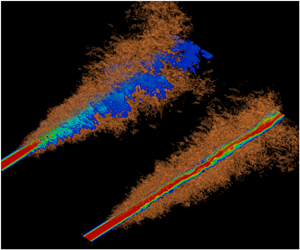
Figure 6 shows vortex structures and gas concentration of the cases with  $u_{sr} = 0.07$ and
  $u_{sr} = 2.1$. The vortex is identified by using the Lambda2 vortex criterion (Jeong & Hussain Reference Jeong and Hussain1995). The identified vortex in figure 6 seems to have more chaotic structures than those reported in many papers regarding jets (Becker & Massaro Reference Becker and Massaro1968; List Reference List1982; Sarikurt & Hassan Reference Sarikurt and Hassan2017) in terms of the presence of coherent structure such as a vortex ring and a horseshoe vortex. The vortical structures of the SR007 case are bounded around the interface between bubbles and ambient fluids. On the other hand, the vortical structures of the SR210 case show dense and narrower distribution. In both cases, vortex breakdown is universally observed by the collapse of the potential core.

Figure 6. Gas concentration fields and isosurfaces of  $\lambda _{2}$ vortices are shown for two different slip ratios, 0.07 and 2.1 (SR007 and SR210). The gas concentration contours of
  $x$–
$x$– $z$ plane are presented. Vortex structures are identified by using Lambda2 vortex criterion. Isosurfaces of vortex structures corresponding to
  $\lambda _{2} = -0.1$ are presented.
3.2. Integral frameworks with 1-D analysis
In this section, the time averaged axial velocity, jet velocity radius and gas concentration radius will be defined and utilised as local variants (as functions of axial coordinate,  $z$) of the 1-D model based on the assumption of Gaussian profiles to predict the evolution of the bubbly jet. Those local variants are obtained from our three-dimensional particle-unresolved DNS, where the bubbly jet naturally evolves and spreads with given viscosity and diffusivity (Reynolds number and Péclet number) in the governing equations (2.4) and (2.5). To reflect these natures in the 1-D model, two more closure models for the entrainment coefficient and spreading rate of gas phase are suggested and will be described in a further text.
The effect of slip velocity on the decaying characteristics of the axial velocity and gas concentration of the bubbly jet along the centreline are compared in figure 7. Figure 7(a) shows the centreline velocity normalised by the inlet velocity  $U_{z0}$, and figure 7(b) shows centreline gas concentration normalised by the inlet gas concentration
  $\varPhi _{b0}$. As shown in figure 7, the presence of the gas phase accelerates the jet and keeps the gas concentration without dispersion up to
  $z = 10D$. Then, all cases with different slip ratios show a decay in the velocity. The single-phase jet, however, keeps its potential core up to
  $z = 15D$. Because the present study has no perturbation at the inlet, the presence of the gas phase results in earlier dispersion of the jet momentum and velocity acceleration until dispersion occurs farther downstream. It accords to the flow characteristics of buoyant jet (Chen & Nikitopoulos Reference Chen and Nikitopoulos1979; Henderson-Sellers Reference Henderson-Sellers1983). It is reported that a lower Froude number condition (large difference between a jet initial temperature and an ambient temperature) of buoyant (thermal) jets results in a higher acceleration of the jet, and the length of the ZFE generally accords to the end of the acceleration. Also, it is reported that a higher Froude number results in an earlier acceleration.

Figure 7. (a) Centreline velocity plotted as a function of downstream distance. (b) Centreline gas concentration plotted as a function of downstream distance.
Based on the assumption of a Gaussian profile and the ratio of conventional length scales between velocity and concentration profiles Morton et al. (Reference Morton, Taylor and Turner1956), the jet velocity and gas concentration can be expressed as
 \begin{gather} U_z (r,z) = U_{zc} \exp({-}r^2/b^2), \end{gather}
 \begin{gather}\varPhi_{b} (r,z) = \varPhi_{bc} \exp({-}r^2/b_{g}^2), \end{gather}
 \begin{gather}b_{g} = \lambda b, \end{gather}
where  $U_{zc}$ is the time-averaged axial centreline velocity of the liquid,
  $\varPhi _{bc}$ is the time-averaged centreline gas concentration,
  $b$ is the
  $1/e$ width of the liquid velocity (jet velocity radius),
  $b_{g}$ is the
  $1/e$ width of the bubble concentration (jet concentration radius) and
  $\lambda$ is the spreading ratio between the bubble concentration and liquid velocity radius. These equations imply that integral properties of the bubbly jet are axisymmetric. From the Gaussian profile assumption, we can derive the volume flux, momentum flux and buoyancy flux as follows:
 \begin{gather} Q(z) = 2{\rm \pi} \int_{0}^{\infty} U_{zc} \exp({-}r^2/b^2) r \,\textrm{d} r = {\rm \pi}U_{zc} b^2, \end{gather}
 \begin{gather}M(z) = 2{\rm \pi} \int_{0}^{\infty} U_{zc}^{2} \exp({-}r^2/b^2) r \,\textrm{d} r = \frac{{\rm \pi} U^2_{zc} b^2}{2}, \end{gather}
 \begin{gather}B(z) = 2{\rm \pi} \int_{0}^{\infty} \beta g \varPhi_{bc} \exp({-}r^2/(\lambda b)^2) r \,\textrm{d} r = {\rm \pi}g' \varPhi_{bc} \lambda^2 b^2, \end{gather}
 \begin{gather} F(z) = 2{\rm \pi} \int_{0}^{\infty} \beta g (U_{zc} \exp({-}r^2/b^2)+u_{sr}) \varPhi_{bc} \exp({-}r^2/(\lambda b)^2) r \,\textrm{d} r \nonumber\\ \hspace{-7.3pc}= {\rm \pi}g' \varPhi_{b} \lambda^2 b^2 \left(\frac{U_{zc}}{1+\lambda^2}+u_{sr}\right), \end{gather}
where  $g'$ is the reduced gravity (
 $g' = \beta g$). In figure 8, the DNS results for the bubbly jets with LSR show good agreement with the Gaussian distributions of the velocity and concentration profiles at all downstream distances. At the height of transition (
 $z = 10D$), all bubbly jets cases still show discrepancy from the Gaussian profiles regarding the velocity and gas concentration. However, cases with HSR still show discrepancy from the Gaussian profiles farther downstream (
 $z = 20D$). It is different from the report on buoyant jets by Chen & Nikitopoulos (Reference Chen and Nikitopoulos1979). In buoyant jets, at the end of ZFE, the potential core of the jet will be eroded by the shear, and the radial distribution of the velocity and buoyancy seems to be Gaussian-like profiles. In the present study, the Gaussian-like distribution of the velocity and gas concentration profile of HSR cases appears around
  $z = 30D$.

Figure 8. Velocity and gas concentration profile with different height. Velocity profiles at  $z = 10D, 20D, 30D, 40D$ (a,c,e,g) and gas concentration profiles at
  $z = 10D, 20D, 30D, 40D$ (b,d,f,h).
From the Gaussian profile assumption, the jet conservation equations, which satisfy entrainment assumption of Morton et al. (Reference Morton, Taylor and Turner1956), are derived as follows:
 \begin{gather} \frac{\textrm{d}({\rm \pi} U_{zc} b^2)}{\textrm{d} z} = 2 {\rm \pi}\alpha U_{zc} b, \end{gather}
 \begin{gather}\frac{\textrm{d}({\rm \pi} U_{zc}^2 b^2)}{\textrm{d} z} = {\rm \pi}g' \varPhi_{bc} (\lambda b)^2. \end{gather}
Equation (3.9) represents the entrainment of ambient fluid into the mean flow of the bubbly jet. Equation (3.10) represents the momentum balance of the bubbly jet. These equations can be rewritten in terms of the volume flux  $Q$, momentum flux
  $M$ and buoyancy
  $B$, respectively, as follows:
 \begin{gather} \frac{\textrm{d} Q_G}{\textrm{d} z} = 2 {\rm \pi}\alpha U_{zc} b, \end{gather}
 \begin{gather}\frac{\textrm{d} M_G}{\textrm{d} z} = B_G. \end{gather}
The subscript  $G$ indicates the Gaussian profile assumption. From (3.9) and (3.10), we can derive the following two ordinary differential equations regarding
  $b$ and
  $U_{zc}$ as functions of
  $z$:
$z$:
 \begin{gather} \frac{\textrm{d}}{\textrm{d} z}(U_{zc}) = \frac{-2 \alpha U_{zc}}{b}+\frac{2Q_{g} g'}{{\rm \pi} U_{zc}/(1+\lambda^2) + u_{sr}}\frac{1}{U_{zc}b^2}, \end{gather}
 \begin{gather}\frac{\textrm{d}}{\textrm{d} z}(b) = 2 \alpha - \frac{Q_{g} g'}{{\rm \pi} U_{zc}/(1+\lambda^2) + u_{sr} }\frac{1}{U_{zc} b}; \end{gather}
the derivation is shown in appendix A. The bubble concentration radius,  $\lambda b$, can be expressed as an exponential function, as follows:
 \begin{equation} \frac{\textrm{d}}{\textrm{d} z}(\lambda b) = \eta_{g} \exp(-\gamma_{\lambda b}u_{sr}), \end{equation}
where  $\eta _{g}$ is the spread rate of the gas phase without any slip velocity in jets.
In buoyant jet experiments, the spread of scalars such as temperature and passive tracers is regarded to be proportional to only the spread rate  $\eta _{g}$ and ranges from 0.101 to 0.156 based on the source condition in previous studies (Fiscehr et al. Reference Fiscehr, List, Koh, Imberger and Brooks1979; Wang & Law Reference Wang and Law2002). In other words, there are no reports on the exponential term of the equation (3.15). In the present study, we considered one more coefficient,
  $\gamma _{\lambda b}$, which is a measure of the effect of the slip ratio of the gas phase. Equation (3.15) shows that the spread of the gas phase exponentially decreases as the slip ratio increases. In the present work, the rate of spread of the gas phase with height is plotted with slip ratio as shown figure 9. It is found that
  $\eta _{g} = 0.080$, which is smaller than what was found in the literature, and
  $\gamma _{\lambda b} = 2.423$.

Figure 9. A curve fitting with an exponential function for each slip ratio case by an assumption that  $\lambda b$ is a linear function of
  $z$.
$z$.
There is an important parameter in the three ordinary differential equations, the entrainment coefficient  $\alpha$. It can be defined as a constant or as a function of other local variables (Morton et al. Reference Morton, Taylor and Turner1956). There have been several efforts to define the local entrainment coefficient because it varies significantly as the bubbly plume develops downstream (Kobus Reference Kobus1968; Ditmars & Cederwall Reference Ditmars and Cederwall1974; Milgram Reference Milgram1983). To define the entrainment coefficient as a local function, Priestley & Ball (Reference Priestley and Ball1955) and List (Reference List1982) suggested using the local Richardson number to define the local entrainment coefficient as follows:
 \begin{equation} \alpha = \alpha_{j} - \left( \alpha_{j}-\alpha_{p} \right) \left( \frac{R}{R_{p}} \right)^2, \end{equation}
where  $\alpha$ is the local entrainment coefficient, which varies with height,
  $\alpha _{j}$ is the entrainment coefficient in the jet-like region,
  $\alpha _{p}$ is the entrainment coefficient in the plume-like region,
  $R$ is the local Richardson number and
  $R_{p}$ is the Richardson number in the plume-like region. The Richardson number represents the ratio between the buoyancy and inertia forces, which reflects the state of the plume in terms of flow development.
Figure 10 shows the Richardson number and the entrainment coefficient. They are calculated based on the Gaussian profile assumption. The Richardson number of the higher slip ratio cases (SR140 and SR210) barely vary with height. This represents that a bubbly jet with a higher slip ratio encounters a limitation in the entrainment of ambient fluid earlier than a bubbly jet with a lower slip ratio. The entrainment coefficient of SR014 does not vary with height in the overall plume-like region. The entrainment coefficient at a lower slip ratio increases in the  $z$-direction. In contrast, the entrainment coefficient at a higher slip ratio decreases in the
  $z$-direction.

Figure 10. (a) Local Richardson number profile by Gaussian profile assumption  $R_{G} = Q_{G}B_{G}/M_{G}^{(5/4)}$ and (b) local entrainment coefficient profile by Gaussian profile assumption with height
  $\alpha _{G} = (\textrm {d} Q_{G}/\textrm {d} z)/(2 {\rm \pi}b U_{zc})$.
The two jet characteristics in figure 10 show monotonic behaviour with respect to the height. Priestley & Ball (Reference Priestley and Ball1955) and List (Reference List1982) related the monotonic behaviour of the entrainment coefficient and Richardson number by introducing the equation (3.16). Therefore, we replaced entrainment coefficients in the equations (3.13) and (3.14) with the equation (3.16) as in the study by Priestley & Ball (Reference Priestley and Ball1955) and List (Reference List1982).
Next, we analysed the bubbly jet after the moment of collapse of the potential core ( $z/D > 24$), i.e. zone of established flow. Direct numerical simulation results at
  $z/D = 24$ were used as the initial conditions of (3.13), (3.14), (3.15) and (3.16). Here
  $\alpha _{j}$ is assumed to be the same as the entrainment coefficient at
  $z/D = 24$ and
  $\alpha _{p}$ and
  $R_{j}$ are assumed to be the values at
  $z/D = 50$.
Figure 11 shows a comparison between the DNS and the solution of the 1-D analysis. As shown in figure 11, the overall predictions shown with solid lines match the bubbly jet DNS results well. As shown in figure 11(c), the gas concentration width of the DNS result follows a linear exponential function (3.15). Figure 11(d) shows that the spreading ratio of the bubbly jet varies with height and ranges from 0.3 to 0.8 downstream. The results show agreement with the results of 0.66–0.69 from a weak bubbly plume experiment by Wang, Lai & Socolofsky (Reference Wang, Lai and Socolofsky2019).

Figure 11. Comparison between 1-D analysis and DNS result: (a) centreline velocity; (b) jet velocity radius; (c) jet concentration width; (d) jet spread rate between gas and liquid (DNS result, symbols; 1-D solution, line).
3.3. Second-order statistics
In this section, normalised second-order statistics of bubbly jets are presented to analyse the effect of slip velocity. The statistics are calculated from our three-dimensional particle-unresolved DNS results with governing equations (2.3), (2.4) and (2.5). Each velocity component (radial, azimuthal and axial velocities) and the gas concentration are decomposed into the mean and fluctuation as  $u_{r} = U_{r} + u'_{r}, u_{\theta } = U_{\theta } + u'_{\theta }, u_{z} = U_{z} + u'_{z}$ and
  $\phi _{b} = \varPhi _{b} + \phi _{b}'$. The time-averaged values such as the Reynolds normal and shear stresses are expressed as
  $\langle u'_{r} u'_{r}\rangle$ and
  $\langle u'_{r} u'_{z}\rangle$. Figure 12 shows the Reynolds normal stresses and shear stresses at
  $z = 20D$ (near field) and
  $z = 40D$ (far field). Each normal stress is normalised with the square of the centreline axial mean velocity.

Figure 12. Reynolds normal stresses and shear stresses of bubbly jet with different slip ratios: (a) radial normal stress at  $z = 20D$; (b) radial normal stress at
  $z = 40D$; (c) azimuthal normal stress at
  $z = 20D$; (d) azimuthal normal stress at
  $z = 40D$; (e) axial normal stress at
  $z = 20D$; (f) axial normal stress at
  $z = 40D$; (g) shear stresses at
  $z = 20D$; (h) shear stresses at
  $z = 40D$.
In figures 12(b) and 12(f), the SR007 case shows that the magnitude of the radial and axial normal stresses reached  $0.038$ and
  $0.061$, respectively. They are comparable with those of other jet cases:
  $0.04$ and
  $0.053$ (Boersma et al. (Reference Boersma, Brethouwer and Nieuwstadt1998), round jet DNS);
  $0.036$ and
  $0.067$ (Wang & Law (Reference Wang and Law2002), round buoyant jet experiment); and
  $0.034$ and
  $0.058$ (Panchapakesan & Lumley (Reference Panchapakesan and Lumley1993), round jet experiment). This result shows that a very small slip velocity does not affect the magnitude of the TKE. But as the slip velocity increases, there are significant differences in the turbulence stress distribution.
It is observed that HSR cases (SR070, SR140 and SR210) have a steep collapse of normal stresses with the radial direction. However, LSR cases (SR007 and SR014) have more Gaussian-like distributions. In the far field, it seems that a HSR promotes rapid collapse, which is consistent with the collapse of the mean axial velocity profile in § 3.2. The radial normal stresses show a peak along the centreline.
An inflection point of the radial normal stress profile is universally observed in the bubbly jet core region. However, steepness around the inflection point varies with slip ratio. Particularly, LSR cases have much flatter and gentle profiles in the bubbly jet core region. The azimuthal and axial normal stresses show similar radial variation, which consists of a peak along the centreline and an off-centre peak. The radial variation of the azimuthal and axial normal stresses varies with the slip ratio in the same way as the variation of the radial normal stress varies.
Figure 12(g) shows the Reynolds shear stress at  $z = 20D$. The off-centre peak with the highest slip ratio (SR210) reached a value of
  $0.018$, which is regularly observed in the far field of the jet in the literature (Panchapakesan & Lumley Reference Panchapakesan and Lumley1993; Boersma et al. Reference Boersma, Brethouwer and Nieuwstadt1998). Low slip ratio cases, however, have off-centre peaks at 0.015 at
  $z = 20D$ yet. In the far field (
 $z = 40D$), the HSR cases keep the magnitude of their Reynolds shear stress, but they skew to the centreline more (figure 12h). Although the peaks of SR007 and SR070 reach 0.018 as well, the peak of SR014 exceeds 0.018. This implies that there is a transition between the slip ratios of 0.14 and 0.7.
Figure 13(a) and 13(b) show the correlations between the gas concentration fluctuation and the radial velocity fluctuation. All cases have an off-centreline peak, and the smaller slip ratio shows a higher magnitude of the peak. This tendency is unlike those with other second-order turbulent characteristics in the present study, which shows that the magnitude of the second-order turbulent characteristics of SR014 is similar to that of SR007 or higher. Cases with HSR have a magnitude that is one order smaller than in the LSR cases. Also, SR007 has a peak value of 0.027, which is comparable with those of other buoyant plume cases: 0.031 (Wang & Law Reference Wang and Law2002); 0.028 (Shabbir & George Reference Shabbir and George1994); and 0.02 to 0.025 (Papanicolaou & List Reference Papanicolaou and List1988).

Figure 13. Turbulent transportation of gas concentration toward each direction: (a) radial direction at  $z = 20D$; (b) radial direction at
  $z = 40D$; (c) azimuthal direction at
  $z = 20D$; (d) azimuthal direction at
  $z = 40D$.
All cases have an off-centre peak in the near field regarding the correlation between the gas concentration fluctuation and the axial velocity fluctuation (figure 13c). In the far field (figure 13d), HSR cases still have a peak in the bubbly jet core region, but LSR cases have a flat profile in the core region. Also, SR007 shows a centreline value of 0.05 for the correlation between the gas concentration and axial velocity fluctuation, which agrees with other buoyant plume and jet results (0.05 Wang & Law Reference Wang and Law2002, 0.05 Papanicolaou & List Reference Papanicolaou and List1988, and 0.056 Shabbir & George Reference Shabbir and George1994).
Figure 14 shows the turbulent gas concentration fluctuation. Low slip ratio cases show a centre peak and collapse in the radial variation of the turbulent gas concentration fluctuation. High slip ratio cases have an off-centre peak of the gas concentration fluctuation in the bubbly jet core region. The location of the peak with HSR almost did not vary with height ( $r/D \sim 0.445$), which is consistent with the location of the peak of the correlation between the gas concentration fluctuation and the velocity fluctuations.

Figure 14. Turbulent gas concentration fluctuation: (a) turbulent gas concentration fluctuation at  $z = 20D$; (b) turbulent gas concentration fluctuation at
  $z = 40D$.
Additionally, it is notable that the location of the peak of the turbulent shear stress is observed at  $r/D \sim 0.55$, which is outside of the location of the peak of the gas concentration fluctuation. Now SR014 shows a higher magnitude of the turbulent gas concentration fluctuation than SR007. This implies that the transitional behaviour observed in second-order turbulent statistics between the slip ratios of 0.14 and 0.7 is due to the gas concentration fluctuation.
3.4. Third-order statistics
Third-order statistics regarding the velocity are important in terms of the contribution to the turbulent diffusion of TKE. Furthermore, third-order statistics regarding the gas concentration play a role in redistributing the gas phase with slip velocity in the flow field. Despite the long time for averaging statistics, third-order statistics do not converge in the bubbly jet core region. In the near field, all slip-ratio cases have a similar magnitude in both the radial and axial turbulent transport. But the radial variation of radial and axial turbulent transports varies with the slip ratio ( figures 15a, 15c, 15e, 16a, 16c and 16e). Peaks of radial and axial turbulent transport are located at 0.04  $r/z$–0.07
  $r/z$. The peak with the highest slip ratio (SR210) is located at 0.04
  $r/z$, and the peak with the lowest slip ratio (SR007) is located at 0.07
  $r/z$. This range is the outer region of locations for peaks of turbulent stresses (0.025
  $r/z$ and 0.042
  $r/z$ for the peaks of the axial normal stress and shear stress of SR210 and SR007, respectively; 0.034
  $r/z$ and 0.04
  $r/z$ for the peaks of the radial and azimuthal normal stresses of SR210 and SR007, respectively).

Figure 15. Turbulent radial transportation of Reynolds normal stresses: (a) radial normal stress at  $z = 20D$; (b) radial normal stress at
  $z = 40D$; (c) azimuthal normal stress at
  $z = 20D$; (d) azimuthal normal stress at
  $z = 40D$; (e) axial normal stress at
  $z = 20D$; (f) axial normal stress at
  $z = 40D$.

Figure 16. Turbulent axial transportation of Reynolds normal stresses: (a) radial normal stress at  $z = 20D$; (b) radial normal stress at
  $z = 40D$; (c) azimuthal normal stress at
  $z = 20D$; (d) azimuthal normal stress at
  $z = 40D$; (e) axial normal stress at
  $z = 20D$; (f) axial normal stress at
  $z = 40D$.
Each directional transport of radial and azimuthal normal stresses has a similar shape of the distribution, but the azimuthal normal stresses always show a lower magnitude of turbulent transport. Taub et al. (Reference Taub, Lee, Balachandar and Sherif2013) reported that the radial turbulent transport of azimuthal normal stresses achieved  $60\,\%$ of the triple moment of the radial velocity fluctuation in their turbulent jet case. Other studies did not quantitatively specify them but reported similar tendencies; that is, the turbulent transport of the azimuthal normal stresses had a lower magnitude than the radial normal stresses (
 $\langle u'^{2}_{\theta }u'_{r}\rangle /\langle u'^{3}_{r}\rangle \sim 51\,\%$ and
  $\langle u'^{2}_{\theta }u'_{z}\rangle /\langle u'^{2}_{r}u'_{z}\rangle \,\sim 69\,\%$ with an experiment on a heated air jet (Darisse, Lemay & Benaïssa Reference Darisse, Lemay and Benaïssa2015);
  $\langle u'^{2}_{\theta }u'_{r}\rangle /\langle u'^{3}_{r}\rangle \sim 54\,\%$ and
  $\langle u'^{2}_{\theta }u'_{z}\rangle /\langle u'^{2}_{r}u'_{z}\rangle \sim 65\,\%$ with DNS on a forced plume Taub et al. Reference Taub, Lee, Balachandar and Sherif2015). The present study also shows
  $\langle u'^{2}_{\theta }u'_{r}\rangle /\langle u'^{3}_{r}\rangle \sim 55\,\%$ and
  $\langle u'^{2}_{\theta }u'_{z}\rangle /\langle u'^{2}_{r}u'_{z}\rangle \sim 66\,\%$ in the far field (
 $z = 40D$).
It is notable that the radial and azimuthal normal stresses in figure 12 have similar magnitude and distribution, but the transport of the azimuthal normal stresses is lower than the radial normal stresses. On the other hand, the turbulent transport of the axial normal stress in the radial direction (figure 15f) is similar to the turbulent transport of the radial normal stress (figure 15b), but the turbulent transport of the axial normal stress in the axial direction (figure 16f) is much higher (2.5–6 times) than the other components. This fact is contrasted with the axial normal stress being just 1.5 times higher than the other components (figure 12).
Regarding the radial transport of the axial normal stress (figures 15e, 15f), all cases have a negative peak next to the centreline. The negative peak reflects that the axial Reynolds normal stress does not diffuse towards the ambient area, but the bubbly jet tends to keep its turbulent energy along the core. A preserved tendency of the TKE is also observed in the turbulent axial transport in figure 16 as negative peaks.
Correlations between the gas concentration fluctuation and Reynolds stresses are shown in figure 17. Most of the correlations near the centreline show negative values or values close to zero. This is consistent with the tendency observed in figures 15 and 16 as negative peaks in the bubbly jet core region. Correlations including the radial and azimuthal velocity components with HSRs have a very small magnitude. Meanwhile, LSR cases have a positive off-centre peak around the core region. It seems that turbulent diffusion toward the ambient area in HSR cases scarcely takes place, but prevails in LSR cases.

Figure 17. Correlation between gas concentration fluctuation and each Reynolds stress: (a) radial normal stress at  $z = 20D$; (b) radial normal stress at
  $z = 40D$; (c) azimuthal normal stress at
  $z = 20D$; (d) azimuthal normal stress at
  $z = 40D$; (e) axial normal stress at
  $z = 20D$; (f) axial normal stress at
  $z = 40D$; (g) shear stress at
  $z = 20D$; (h) shear stress at
  $z = 40D$.
The correlation between the gas concentration fluctuation and the Reynolds shear stress regularly shows a negative peak in the bubble core region and a positive peak around the bubble core for all cases (figures 17g, 17h). The magnitude of the positive peak with very HSR is not comparable to the magnitude of the LSR cases. On the other hand, the magnitude of the negative peak is comparable to the magnitude of the LSR cases. Also, the peak is located in the innermost position ( $r/z - 0.008$), where the negative peak of the radial transport of the axial normal stress occurs (in other words, the axial transport of Reynolds shear stress). This implies that the fluctuation of the concentration has strong relation with the axial fluctuations in regards to the correlation with Reynolds shear stresses.
3.5. TKE budget
We plotted the TKE budget of the bubbly jet in the near field and far field to investigate how the bubbles contribute to the turbulent process in the bubbly jet. The transport equation of the TKE is arranged from the momentum equation and the assumption on the axisymmetric jet flow and written as follows:
 \begin{align} 0
&={-}\left[U_{r}\frac{\partial k}{\partial r} +
U_{z}\frac{\partial k}{\partial z}\right] -
\left[\frac{1}{r} \frac{\partial}{\partial r} \left(r
\overline{u'_{r}p'} \right) + \frac{\partial}{\partial z}
\left(\overline{u'_{z}p'} \right)\right] \nonumber\\ &\quad
-\left[\overline{u'_{r}u'_{r}}\frac{\partial
U_{r}}{\partial r} + \overline{u'_{z}u'_{z}}\frac{\partial
U_{z}}{\partial z} + \overline{u'_{r}u'_{z}} \left(
\frac{\partial U_{r}}{\partial z} + \frac{\partial
U_{z}}{\partial r} \right) +
\frac{\overline{u'_{\theta}u'_{\theta}}U_{r}}{r} \right]
\nonumber\\ &\quad -\left[\frac{1}{r}
\frac{\partial}{\partial r} \left(r \overline{u'_{r}k}
\right) + \frac{\partial}{\partial z}
\left(\overline{u'_{z}k} \right)\right] - \frac{1}{Re}
\left[ \frac{1}{r} \frac{\partial}{\partial r} \left(
r\frac{\partial k}{\partial r}\right) + \frac{\partial^2
k}{\partial z^2}\right] \nonumber\\ &\quad - \frac{1}{Re}
\left[ \overline{ \left( \frac{\partial u'_{r}}{\partial r}
\right)^2} + \overline{ \left( \frac{\partial
u'_{\theta}}{\partial r} \right)^2} + \overline{ \left(
\frac{\partial u'_{z}}{\partial r} \right)^2} + \overline{
\left( \frac{\partial u'_{r}}{\partial z} \right)^2} +
\overline{ \left( \frac{\partial u'_{\theta}}{\partial z}
\right)^2} + \overline{ \left( \frac{\partial
u'_{z}}{\partial z} \right)^2} \right. \nonumber\\ &\quad +
\frac{ \overline{u'_{r}u'_{r}}} {r^2} + \left.
\vphantom{\overline{ \left( \frac{\partial u'_{r}}{\partial
r} \right)^2}} \frac{ \overline{u'_{\theta}
u'_{\theta}}}{r^2} \right] + Ri \left[ \overline{u'_{z}
\phi'_{b} } \right], \end{align}
\begin{align} 0
&={-}\left[U_{r}\frac{\partial k}{\partial r} +
U_{z}\frac{\partial k}{\partial z}\right] -
\left[\frac{1}{r} \frac{\partial}{\partial r} \left(r
\overline{u'_{r}p'} \right) + \frac{\partial}{\partial z}
\left(\overline{u'_{z}p'} \right)\right] \nonumber\\ &\quad
-\left[\overline{u'_{r}u'_{r}}\frac{\partial
U_{r}}{\partial r} + \overline{u'_{z}u'_{z}}\frac{\partial
U_{z}}{\partial z} + \overline{u'_{r}u'_{z}} \left(
\frac{\partial U_{r}}{\partial z} + \frac{\partial
U_{z}}{\partial r} \right) +
\frac{\overline{u'_{\theta}u'_{\theta}}U_{r}}{r} \right]
\nonumber\\ &\quad -\left[\frac{1}{r}
\frac{\partial}{\partial r} \left(r \overline{u'_{r}k}
\right) + \frac{\partial}{\partial z}
\left(\overline{u'_{z}k} \right)\right] - \frac{1}{Re}
\left[ \frac{1}{r} \frac{\partial}{\partial r} \left(
r\frac{\partial k}{\partial r}\right) + \frac{\partial^2
k}{\partial z^2}\right] \nonumber\\ &\quad - \frac{1}{Re}
\left[ \overline{ \left( \frac{\partial u'_{r}}{\partial r}
\right)^2} + \overline{ \left( \frac{\partial
u'_{\theta}}{\partial r} \right)^2} + \overline{ \left(
\frac{\partial u'_{z}}{\partial r} \right)^2} + \overline{
\left( \frac{\partial u'_{r}}{\partial z} \right)^2} +
\overline{ \left( \frac{\partial u'_{\theta}}{\partial z}
\right)^2} + \overline{ \left( \frac{\partial
u'_{z}}{\partial z} \right)^2} \right. \nonumber\\ &\quad +
\frac{ \overline{u'_{r}u'_{r}}} {r^2} + \left.
\vphantom{\overline{ \left( \frac{\partial u'_{r}}{\partial
r} \right)^2}} \frac{ \overline{u'_{\theta}
u'_{\theta}}}{r^2} \right] + Ri \left[ \overline{u'_{z}
\phi'_{b} } \right], \end{align}
where,
 \begin{equation} k = \tfrac{1}{2} \left( \overline{u'^2_{r} + u'^2_{\theta} + u'^2_{z}} \right). \end{equation}
 By using the axisymmetric assumption, terms including the azimuthal differentiation, odd number of azimuthal elements and mean azimuthal velocity elements are eliminated. The terms separated by square brackets in (3.17) represent the transport of TKE by the mean flow (advection term), the transport of TKE by pressure (pressure strain term), the production by the mean shear and mean flow (production term), the transport of TKE by Reynolds stress (turbulent transport term), the transport of TKE by viscous stress (viscous transport term), the rate of dissipation (dissipation term) and the production by buoyancy (buoyancy production term). The dissipation term is obtained as a closing term of the budget. Each term is plotted in figures 18, 19 and 20. The terms are normalised by  $U_{zc}^3 / z$.

Figure 18. Turbulent kinetic energy budget terms at different height: (a) advection at  $z = 20D$; (b) advection at
  $z = 40D$; (c) pressure strain at
  $z = 20D$; (d) pressure strain at
  $z = 40D$.

Figure 19. Turbulent kinetic energy budget terms at different height: (a) production at  $z = 20D$; (b) production at
  $z = 40D$; (c) buoyancy production at
  $z = 20D$; (d) buoyancy production at
  $z = 40D$.

Figure 20. Turbulent kinetic energy budget terms at different height: (a) turbulent diffusion at  $z = 20D$; (b) turbulent diffusion at
  $z = 40D$; (c) dissipation at
  $z = 20D$; (d) dissipation at
  $z = 40D$.
Advection and pressure strain in the bubbly jet seem to be the most unstable terms among the TKE budget terms in the present study. The advection term has a positive peak along the centreline and a negative peak around the bubbly jet core region (figure 18a). The negative peak persists in the far field. The positive peak along the centreline comes from the mean axial advection of the TKE, and the negative peak comes from entrainment of the ambient fluid in the shear layer of the bubbly jet. But oscillations of the centreline value along the centreline are observed in figure 18(b). For example, SR007 and SR014, which have similar jet structure in the present study, show inconsistency in the magnitude of centreline value. Also SR210 has a negative peak in the centre of the jet, while SR070 and SR140 have a positive peak in the centre of the jet. This might come from very large spatial and temporal motion such as plume meandering (Simiano & Lakehal Reference Simiano and Lakehal2012).
As shown in figures 18(c) and 18(d), the pressure strain term of HSR cases has an off-centre peak, but the peak of the LSR cases oscillates in the far field (e.g. SR007 of figure 18d). The magnitude of the pressure strain in the near field is not more significant than the advection. In the far field, however, it is more dominant than the advection in HSR cases. The magnitude of the pressure strain has a distinctive peak along the centreline in the far field.
Figure 19 shows the production and buoyancy production terms. In the near field, the production is almost one order of magnitude higher than the buoyancy production. In the far field, this difference is reduced by five times. Generally, the peak of the production is observed around the bubbly jet core region and shows an accordance with the location of the peak of the buoyancy production. This is in contrast with the experimental result from a weak bubble plume, which shows a very high contribution of bubbles to the production of TKE but negligible contribution of water (Lai & Socolofsky Reference Lai and Socolofsky2019). The experiment was buoyancy dominated flow, so it resulted in low mean kinetic energy and mean shear. Therefore, its TKE production probably depends on bubble induced turbulence. Furthermore, interfacial characteristics and deformation of the bubbles can be attributed to buoyancy production in terms of pressure fluctuation and viscous forces (Nguyen et al. Reference Nguyen, Bae, Euh, Song and Yun2012; Santarelli et al. Reference Santarelli, Roussel and Fröhlich2016).
Regarding the buoyancy production, LSR cases show flat radial distribution in the bubbly jet core region, and HSR cases show a peak with a non-zero centreline value. In the near field, all cases show similar magnitude of the buoyancy production, but LSR cases have a wider radial distribution. In the far field, the buoyancy production has two to three times higher magnitude than the magnitude in the near field. The location of the peak of SR140 and SR210 is almost in accordance with the jet concentration radius (figure 11c). This result shows the formation of a rigid jet core in HSR cases, and the buoyancy production takes place around the bubbly jet core interface.
Figure 20 shows the turbulent diffusion and dissipation terms. The turbulent diffusion profile typically consists of a positive peak along the centreline, a negative off-centre peak, and a very small positive peak around the shear layer of the bubbly jet. In the near field, the magnitude of the turbulent diffusion is bounded between  $+$0.12 and
  $-$0.12. In the far field, there is a negative peak of around
  $-$0.24 for the HSR cases. Like the pressure strain term, LSR cases have an irregular peak along the centreline, but HSR cases regularly have a positive peak along the centreline. The distribution of the dissipation of the TKE is similar to the TKE in figure 12. Most of the dissipation occurs in the bubble core region and rapidly decreases in the outer region of the bubble core.
4. Conclusion
Bubbly jets with five different slip ratios were simulated using DNS. We chose bubble slip velocities that vary from a very small value ( $7\,\%$ of the inlet velocity) to a very high value (
 $210\,\%$ of the inlet velocity). The effect of the slip velocity on the bubbly jet was studied with three different perspectives: (1) a comparison on instantaneous flow fields between HSR cases and LSR cases; (2) an integral framework with 1-D analysis; and (3) a statistical analysis with higher-order terms and the turbulent kinetic energy budget.
First of all, the single-phase jet case is validated by comparing with the literature data. After adding the gas concentration at the inlet of the bubbly jet, we found that a transition point where the breakdown of the potential core occurs with the gas phase is observed earlier than without the gas phase. There was a negligible effect of the slip ratio on the position of the transition point, but various structural differences were observed after the transition point. High slip ratio cases keep their rigid bubbly jet core, but a gas phase with LSRs is dispersed into ambient in the form of a bubble swarm or lump.
The time-averaged spread of the gas phase was assumed to follow an exponential function that includes the slip ratio as an exponent. Ordinary differential equations regarding the axial velocity and spread of the velocity radius were derived from conservation equations with a conventional assumption about the round jets and plumes (Morton et al. Reference Morton, Taylor and Turner1956). The local entrainment coefficient was obtained from the relationship with the local Richardson number (Priestley & Ball Reference Priestley and Ball1955; List Reference List1982). The axial velocity, velocity radius and gas concentration radius were predicted very well downstream of the bubbly jets.
From the analysis of the second-order statistics, it was observed that a HSR results in the prevention of diffusion of the gas phase and forms a rigid bubbly jet core along the centreline. Correlations including the gas concentration fluctuation show a peak inside the location of the peak of turbulent stresses. The normalised magnitudes of the turbulent stresses were similar in each case and comparable with those of a single-phase jet and plume in the literature. However, the distribution was narrower in HSR cases. Furthermore, the correlation between the radial velocity fluctuation and gas concentration fluctuation was severely suppressed in HSR cases. But the autocorrelation of the gas concentration fluctuation or correlations between the axial velocity fluctuation and gas concentration fluctuation were strong in the bubbly jet core region with a HSR.
From the analysis of the third-order statistics, the smallest turbulence structure of the HSR case was observed at  $r/z \sim 0.008$ in the form of a negative peak of the axial transport of Reynolds shear stresses and the correlation between the Reynolds shear stress and gas concentration fluctuation. In the analysis of the TKE budget, the advection and the production terms showed similar distributions to what was observed in conventional jets and plumes. However, turbulent diffusion and pressure strain terms showed a positive peak along the centreline, which was not reported for single-phase jets and plumes. The buoyancy production generated by bubbles is two to three times more dominant in the far field than in the near field.
Funding
This work was supported by the National Research Foundation of Korea (NRF) grant, which is funded by the Korean government (MSIT) (NRF-2018-Global PhD Fellowship Program, no. 2020R1A5A8018822 and 2021R1A2C2012469).
Declaration of interests
The authors report no conflict of interest.
Appendix A
In this appendix, we derive the ordinary differential equations for the jet centreline velocity and jet velocity radius. These properties are derived from conservation equations for round jets and plumes regarding the volume flux, momentum flux and buoyancy flux. In fully developed flows, the buoyancy flux  $F_G$ is constant under the Boussinesq approximation and can be expressed with the inlet buoyancy flux
  $F_{G0}$ as
 \begin{equation} F_{G0} = Q_{g0} g'. \end{equation}
Here,  $Q_{g0}$ is the volume flux of the gas phase at the source. The general form of the buoyancy flux with the Gaussian profile assumption is expressed in (3.8). You can find overlapped expressions (
 ${\rm \pi} g' \varPhi _{bc} (\lambda b)^2$) in (3.8) and (3.10). The right-hand side of (3.10) can replace the same expression in (3.8), i.e.
 \begin{align} F(z) &= F_{G0} = Q_{g0} g' \nonumber\\ &= \frac{\rm \pi}{2} \frac{\textrm{d}}{\textrm{d} z}(U_{zc}^2 b^2)\left( \frac{U_{zc}}{1+\lambda^2}+u_{sr} \right). \end{align}
This equation can be rearranged by putting the derivative term on the left-hand side, i.e.
 \begin{equation} \frac{\textrm{d}}{\textrm{d} z}(U_{zc}^2 b^2) = \frac{2}{\rm \pi} \frac{Q_{g0}g'}{U_{zc}/(1+\lambda^2) + u_{sr}}. \end{equation}
For further derivation, we should recall continuity equation (3.9), namely
 \begin{equation} \frac{\textrm{d}({\rm \pi} U_{zc} b^2)}{\textrm{d} z} = 2 {\rm \pi}\alpha U_{zc} b. \end{equation}
By the product rule of the derivative, (A3) can be separated into two parts of the derivatives, as follows:
 \begin{equation} \frac{\textrm{d}}{\textrm{d} z}(U_{zc}^2 b^2) = \frac{\textrm{d}}{\textrm{d} z}(U_{zc})(U_{zc}b^2)+ \frac{\textrm{d}}{\textrm{d} z}(U_{zc}b^2)(U_{zc}), \end{equation}
where  $\textrm {d}(U_{zc}b^2)/\textrm {d} z$ is already known as (A4). Then, the equation can be rearranged for
  $\textrm {d}(U_{zc})/\textrm {d}(z)$ as follows:
 \begin{equation} \frac{\textrm{d}}{\textrm{d} z}(U_{zc}) = \left[{-}U_{zc} \frac{\textrm{d}}{\textrm{d} z}(U_{zc}b^2) + \frac{\textrm{d}}{\textrm{d} z}(U_{zc}^2b^2) \right]/(U_{zc}b^2). \end{equation}
This equation is the same as (3.13). In the same way,  $\textrm {d}(b)/\textrm {d} z$ can be expressed as follows:
 \begin{align} \frac{\textrm{d}}{\textrm{d} z}(b) &= \left[ \frac{\textrm{d}}{\textrm{d} z}(U_{zc}b^2) - \frac{\textrm{d}}{\textrm{d} z}(U_{zc}b)b \right]/(U_{zc}b) \nonumber\\ &= \left[ \frac{\textrm{d}}{\textrm{d} z}(U_{zc}b^2) - \frac{\textrm{d}}{\textrm{d} z}(U_{zc}^2b^2)/(2U_{zc}b) \right]/(U_{zc}b) \nonumber\\ &= 2\alpha - \frac{Q_{g0} g'}{{\rm \pi} U_{zc}^2b (U_{zc}/(1+\lambda^2)+u_{sr}}. \end{align}


