


1. Introduction
Planetary entry occurs at very high velocities: in excess of 10 km s $^{-1}$ is typical for Lunar return. At such speeds, a strong bow shock forms ahead of the vehicle. This is advantageous, as it provides sufficient drag to enable deceleration of the craft until parachutes may be safely deployed. However, the compression of the gas through this shock results in very high temperatures (above 10 000 K for the aforementioned Lunar return case), leading to substantial heat fluxes to the vehicle surface. Further, at such temperatures there are significant thermochemical changes in the flow, notably dissociation, ionisation and the formation of new radical species (Gnoffo Reference Gnoffo1999). The high temperature gas also produces intense electromagnetic emission, which can result in large radiative heat fluxes. For large nose radii, this can be the dominant source of vehicle heating (Brandis & Johnston Reference Brandis and Johnston2014). Furthermore, many of these thermochemical processes occur on time scales comparable to those of the flow. Large parts of the flow field may thus be in thermal and/or chemical non-equilibrium, which significantly complicates engineering analysis. Understanding this complex environment – which couples compressible flow physics, non-equilibrium thermochemistry and quantum theories of radiation – is a key objective of aerothermodynamics research.
One important source of ground test data relevant to these problems is high-enthalpy shock tube experiments. In such studies, a normal shock is passed through a quiescent test gas at a chosen density and composition of interest. The gas in the compressed test slug can then be used as an analogy to that along the stagnation streamline of an entry vehicle, allowing estimates of radiative heating (as well as the thermochemical state at the edge of the boundary layer) to be made (Park Reference Park1989). This experimental approach has the advantage of exactly replicating the conditions experienced during flight, with no dimensional scaling required. Typically, measurements are made optically using either emission or absorption techniques. This is done either through windows in the tube wall (Cruden et al. Reference Cruden, Martinez, Grinstead and Olejniczak2009) or as the shock emerges from the end of the tube (Brandis et al. Reference Brandis, Morgan, McIntyre and Jacobs2010b). This data can be used to either directly estimate the radiative heat flux on the vehicle surface, or to infer species populations and, hence, chemical-kinetic or radiative excitation rates (Danehy et al. Reference Danehy, Bathel, Johansen, Winter, O'Byrne and Cutler2013). The experimental results extracted from these facilities can then be used to inform computational model development and to validate their predictions.
Although simple in principle, actual shock tube experiments are complicated by several realities. The most challenging is perhaps to achieve the correct shock speed, as the characteristics of the post-shock gas are very sensitive to this parameter (Brandis & Johnston Reference Brandis and Johnston2014). Pressure waves from the driver section (Stalker Reference Stalker1967) and diaphragm opening processes (White Reference White1958) both modulate the shock speed profile along the length of the tube. In addition, the growth of a wall boundary layer behind the shock front causes attenuation of the shock speed through a mechanism known as the Mirels effect (Mirels Reference Mirels1963). Here, mass loss into the near-wall region causes test gas to flow around the contact surface; there is thus a reduction in the accumulated mass within the test slug which reduces the shock speed and limits the achievable test time.
An open question in the literature is: to what extent do such variations in shock speed matter to these shock tube experiments? Light (Reference Light1973) considered this problem from the following perspective: in investigations of chemical kinetics, the rate parameters (which are the measurement objective) are functions of pressure and temperature. In arc-driven shock tubes, the rapid decrease in driver pressure caused decelerations far above those stemming from the Mirels effect. For the shock to decelerate to such a degree, strong expansion waves must reduce the pressure throughout the test slug and, thus, this should change the apparent chemical-kinetic rates.
To investigate the impact of shock deceleration, Light (Reference Light1973) measured the electron density behind strong shock waves using a microwave interferometer. His results show differences in the observed trends of electron density through the shock layer at the varied conditions. However, the main mechanism of shock speed modulation between tests was to change the initial fill pressure in the tube. The presented results are thus at very different pressures, and the final shock speeds are also not equivalent. These factors, in combination with an overall poor agreement with a numerical model of the temperature variation in the test gas, has meant that these results have not convincingly proven any direct link.
The leading shock tube facility in the field of aerothermodynamics is the electric arc shock tube (EAST) at NASA Ames. This facility has produced a large body of data for the majority of current or future missions under consideration today (Cruden, Prabhu & Martinez Reference Cruden, Prabhu and Martinez2012; Brandis et al. Reference Brandis, Johnston, Cruden and Prabhu2017; Cruden & Bogdanoff Reference Cruden and Bogdanoff2017; Cruden & Brandis Reference Cruden and Brandis2020). In several test campaigns undertaken at EAST, shock deceleration has been posited as a potential source of disagreement between the experimental results and numerical predictions. There, changes in shock speed on the order of kilometres per second are common along the length of the facility. Notably, Cruden (Reference Cruden2012) measured electron densities in the shock layer across a range of conditions, showing values significantly in excess of equilibrium. In a cross-facility comparison study, Brandis et al. (Reference Brandis, Cruden, Prabhu, Bose, McGilvray and Morgan2010a) proposed shock deceleration as a potential cause of excess radiation in the EAST data. This mechanism is shown diagrammatically in figure 1, wherein the changing shock speed leads to a gradient in enthalpy (and, hence, temperature) through the test slug. An improved agreement was seen in trends of background continuum radiation if this effect was modelled, but again a fully convincing argument was not possible.
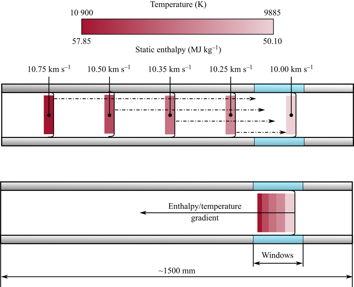
Figure 1. Diagram demonstrating the effect of shock deceleration on post-shock equilibrium in the EAST facility. The upper diagram shows the variation in shock speed and the downstream movement of the shocked gas. The lower diagram represents the test slug as imaged when the shock is at the observation window. Adapted from Brandis et al. (Reference Brandis, Cruden, Prabhu, Bose, McGilvray and Morgan2010a).
Partly in an effort to investigate the shock deceleration influence, several authors have attempted computational simulations of EAST. However, the large aspect ratio of shock tube facilities makes full, viscous simulations incorporating thermochemistry extremely expensive (Kotov et al. Reference Kotov, Yee, Panesi, Prabhu and Wray2014). In the two most recent attempts, one suffered from numerical issues (Bensassi & Brandis Reference Bensassi and Brandis2019); this reflects the challenging nature of these simulations. The second successfully simulated the test slug, but because the driver was not fully modelled the shock deceleration trajectory was not reproduced (Chandel et al. Reference Chandel, Nompelis, Candler and Brandis2019). One-dimensional simulation approaches have also been inconclusive (Sharma Priyadarshini et al. Reference Sharma Priyadarshini, Munafo, Brandis, Cruden and Panesi2018).
More recently, a new computational tool by Satchell, McGilvray & Di Mare (Reference Satchell, McGilvray and Di Mare2022b) – Lagrangian shock tube analysis (LASTA) – has been developed to investigate the problem of shock deceleration. This methodology uses the experimentally measured shock speed profile as an input, circumventing the challenge of reproducing the shock trajectory accurately via simulation. Through this analysis, it was demonstrated that the changing strength of the shock will generate an entropy gradient in the test slug; this persists despite pressure changes (notably, caused by relaxation waves associated with the decelerating shock) in the gas and, consequently, so does a temperature variation. This result has been validated against data from the T6 aluminium shock tube, where it was shown to accurately predict increases in stagnation-point heat flux due to temperature gradients in the slug caused by shock deceleration (Satchell et al. Reference Satchell, Glenn, Collen, Penty-Geraets, McGilvray and Di Mare2022a). This new modelling approach has not yet been applied in the case of radiating shock-layer experiments.
This work aims to conclusively confirm the importance of this shock deceleration effect for high-enthalpy shock tube tests. This is achieved through a combined experimental and numerical approach: first, different shock trajectories are generated experimentally. These end at the same shock speed, and are produced in identical initial shock tube fill densities and compositions. The generated post-shock conditions are thus nominally identical. For each of these cases, the post-shock trends in either radiation or electron densities are measured. Any differences between the observed variations of these properties in the test slug can thus be attributed to shock speed variations upstream of the measurement location. To further strengthen this link, the observed trends are then compared with the predictions of LASTA. This code explicitly accounts for the influence of the shock trajectory, thereby allowing the contribution of the variation in shock speed to be assessed.
This paper begins by first describing the ground test facility and the emission spectroscopy system used for these experiments in § 2. This is followed by a brief description of the numerical analysis methodology in § 3. The method by which differing shock trajectories may be produced in this type of shock tube, as well as the rationale for the selection of the test conditions, is given in § 4. Experimental results for the variation in atomic oxygen emission with distance behind the shock are then shown in § 5, with comparisons made to numerical predictions. These results are complimented by a numerical study in § 6 to explain the observed trends. The results of a similar analysis considering variations in electron density are then discussed in § 7. Finally, § 8 summarises the key conclusions of the paper and provides suggestions for how these findings may be used to improve experiments conducted in similar shock tube facilities in the future.
2. Experimental details
This section details the key attributes of the experimental portion of this work. A summary of the ground test facility and its operation are first provided. The particulars of the emission spectroscopy system – the key experimental measurement in this work – are then discussed.
2.1. Facility overview
The experiments described herein were conducted in the University of Oxford T6 stalker tunnel. This is a free-piston driven, multimode, transient, high-enthalpy ground test facility. It is described in detail by Collen et al. (Reference Collen2021). As such, only a brief overview of the design and operation of the tunnel is given here.
In this work, the facility was operated in its aluminium shock tube (AST) mode. A diagram of T6 in this configuration is given in figure 2. Before an experiment, a 36 kg piston is initially held at the upstream end of the compression tube. Here, it separates high-pressure reservoir air (at 2600 kPa) from the pure helium ‘driver’ gas (at 35 kPa) in the compression tube. A 2 mm thick, scored, 304 2B grade stainless steel diaphragm at the downstream end of this section isolates this driver gas from the shock tubes. At the beginning of the test, the piston is released; it rapidly accelerates to velocities in excess of 100 mm s $^{-1}$, causing a polytropic compression of the driver gas. At approximately 46 MPa, the primary diaphragm ruptures; this allows the compressed helium to expand through an orifice plate into the shock tube sections, driving a normal shock downstream. The continued forward motion of the piston sustains compression of the driver gas, preventing the generation of expansion waves which would otherwise attenuate the shock. Simultaneously, the piston is slowed by the high driver gas pressure which allows it to be safely caught by nylon buffers at the end of the compression tube.
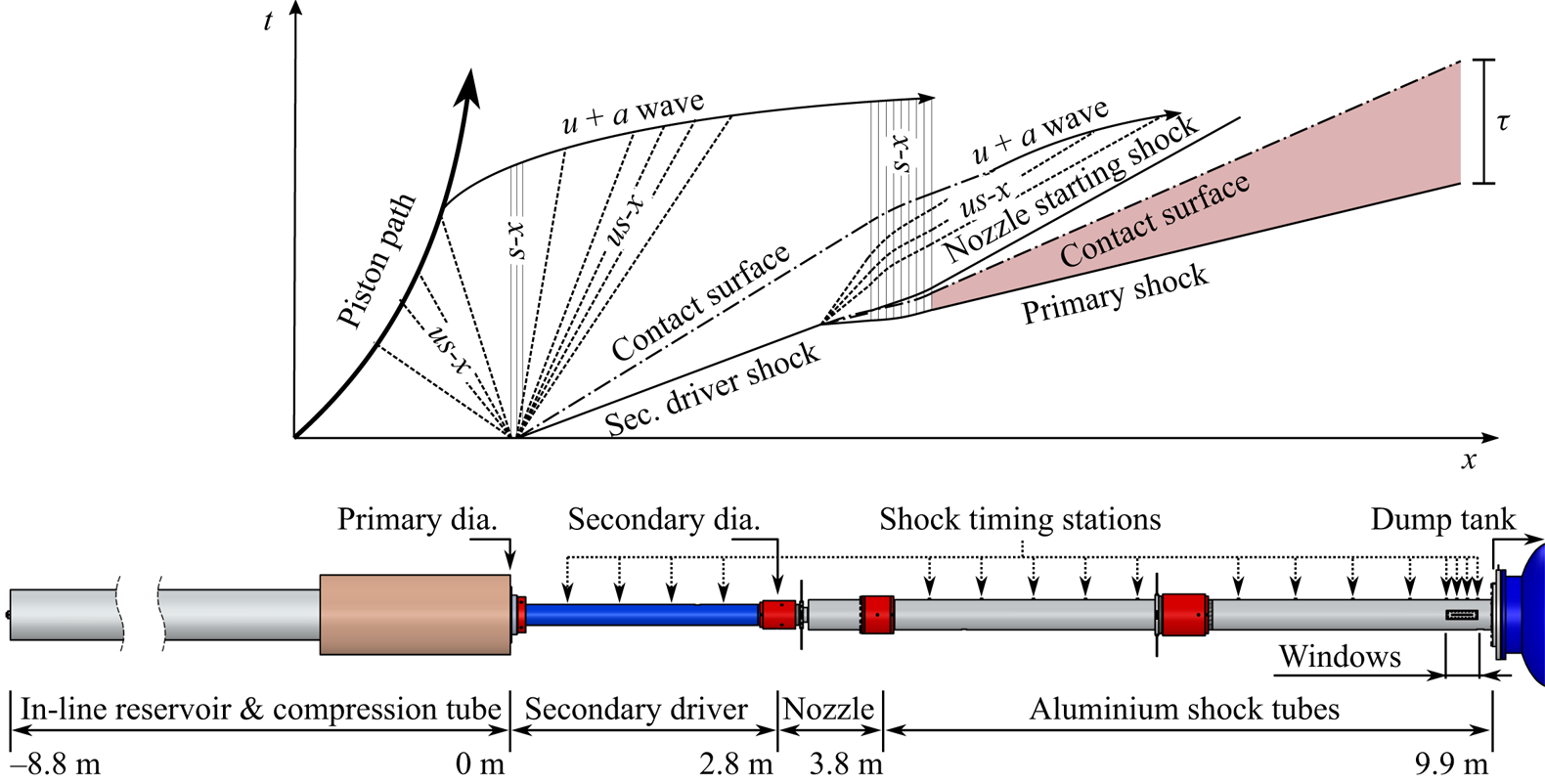
Figure 2. Diagram of T6 in AST mode, including a distance–time diagram of the main wave processes which occur during a test. Unsteady expansions are denoted ‘us-x’ and steady expansion regions by ‘s-x’. The valid test flow is marked in red and the nominal test time by ‘ $\tau$’.
Immediately following the primary diaphragm is the secondary driver, with a diameter of 96.3 mm. Depending on the desired shock speed properties, this can either form a single volume with the AST section or be filled with helium and separated from the nozzle with a Mylar secondary diaphragm. The specifics of this section are discussed in more detail in § 4.1. At the upstream end of the AST, a 12 $^{\circ }$ nozzle increases the tube diameter to 225 mm; this both extends the integration path length for optical techniques and reduces the influence of the wall boundary layer. The latter can both cause attenuation of the shock (as described in the analysis of Mirels Reference Mirels1963) and results in radial non-uniformities in the test gas. Test time is also increased by using a larger tube bore, being quadratic in diameter (Mirels Reference Mirels1964). However, the increase in diameter also causes a performance loss (i.e. a reduction in primary shock speed) due to the further expansion of the driver gas through the nozzle. This slower primary shock then processes the test gas as shown in figure 2; the resultant region of valid test flow is highlighted in red. Also shown is the passage of a nozzle starting shock (moving upstream in the primary shock reference frame). This forms due to the transient start-up processes in the nozzle, as described by Smith (Reference Smith1966); this does not directly affect the test gas.
Located at the downstream end of the AST (approximately 9.5 m from the primary diaphragm) are two diametrically opposed optical windows. These are either 190 mm or 200 mm long, oriented in the axial direction (i.e. perpendicular to the shock front) and permit optical access for a variety of measurement techniques. In this work, an optical emission spectroscopy system is located at this position. This is discussed further in § 2.2.
Shock speed variation (SSV) is measured in the facility using time-of-flight calculations between flush-mounted pressure transducers in the tube wall. In this work, the sensors used were PCB piezotronics 113B series piezoelectric transducers. These are distributed along the secondary driver and AST sections (as shown in figure 2) to allow rebuilding of the shock trajectory as it travels along the facility. The uncertainty in the shock speed measurement is determined using the approach of James et al. (Reference James, Gildfind, Lewis, Morgan and Zander2018), which includes the contribution of the spatial and temporal uncertainty to the measurement. In this work, the spatial uncertainty (which is made up of the manufacturing tolerance in sensor position and the uncertainty due to the physical extent of the transducer) is taken as 2 mm. The temporal uncertainty is comprised of a contribution from the sampling rate of the data acquisition system (2 MHz for these experiments) and the uncertainty in the shock arrival time. The latter is determined by manual identification of the start and end of the pressure step associated with shock arrival. This places a conservative maximum uncertainty bound on the mean shock speed between each measurement location.
2.2. The optical emission spectroscopy system
The primary measurement used in this work is performed using the optical emission spectroscopy arrangement shown in figure 3. The facility is typically operated using a dual-channel emission system, in which the ultraviolet and visible/near-infrared regions are measured simultaneously. For the experiments reported here, only data from the visible/near-infrared spectrometry system are presented; as such only this is described in detail. A diagram of this arrangement is shown in figure 3. The purpose of the emission system is to capture spatially and spectrally resolved emission from behind the normal shock. This is achieved by coupling an Andor iStar sCMOS intensified camera, with a Gen 2 W-AGT photocathode and P46 phosphor, to a Princeton Instruments Isoplane-320 diffraction grating spectrograph. The camera was gated at 500 ns to minimise spatial blurring of the shock during the exposure time. For the oxygen emission measurements discussed in § 5.2, a relatively coarse grating of 150 grooves mm $^{-1}$, blazed at 500 nm, was used. This was set to a central wavelength of 730 nm. For the electron density experiments in § 7, a fine grating of 1200 grooves mm
 $^{-1}$ was used to minimise instrument broadening. This was also blazed at a wavelength of 500 nm and was set to a central wavelength of 656.6 nm.
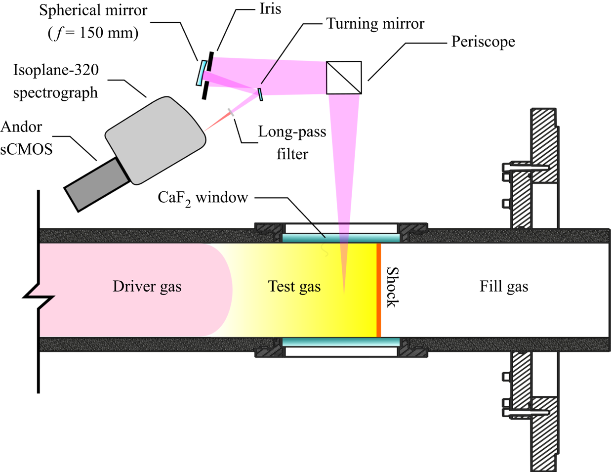
Figure 3. Diagram of emission spectroscopy arrangement at the AST windows. Not to scale.
Radiative emission from the post-shock gas is imaged onto the spectrograph using a 150 mm focal length spherical mirror. A periscope (consisting of two 50 mm diameter flat mirrors) accounts for the difference in height between the spectrograph slit and the tunnel, and provides rotation of the beam. An additional turning mirror minimises the incident light angle on the spherical mirror, reducing coma. All optical components were Thorlabs protected silver (-P01 series) with a guaranteed average reflectance greater than 97.5 % in the range 450 nm to 2000 nm. A 550 nm long-pass filter (Thorlabs FEL0550) was included in the optical path to prevent the imposition of higher-order spectral features on the measured spectra. Finally, an iris (set to 20 mm diameter) was used to tune the depth-of-field characteristics of the optical system. This is critical due to the substantial spatial gradients in properties behind the shock. The measured object and imaging distances were 1856 mm and 154.4 mm, respectively. This arrangement gave a maximum spot size (or ‘circle of confusion’) at the tube wall of 1.14 mm. The field-of-view was determined to be approximately 160 mm along the axis of the tube.
The spectroscopy system was calibrated using an absolute standard of spectral radiance. The approach used here closely follows the methodology of Cruden (Reference Cruden2014) and is described fully by Collen (Reference Collen2021). In summary, a Bentham Instruments SRS8 quartz-tungsten-halogen integrating sphere with spectral radiance calibration in the range 300 nm to 2500 nm is used. This has an outlet diameter of 50 mm and so several overlapping images must be taken as the source is translated along the field-of-view. This in situ calibration approach has the advantage of accounting for all losses in the optical system (for example, due to reflectance of the optical surfaces or vignetting) directly. Using the known emission of the lamp, this can be used to convert the measured raw signal on the camera (in units of signal counts) to a meaningful value of spectral radiance (in W cm $^{-2}$ sr
 $^{-1}\ \mathrm {\mu }$m
 $^{-1}$). This allows direct comparison to numerical tools. The calibration process is completed prior to every test. Immediately before the calibration, the windows are also cleaned with acetone to ensure they are free from any traces of the post-test residue which accumulates on the tube wall.
The spatial and wavelength dimensions of the detector also require calibration. The former was achieved by placing a back-illuminated plate with precision-machined holes on the tube centreline. This allows the pixel positions of the holes in the resulting image to be related to their physical spacing, giving a relation between pixels and spatial position (i.e. pixels per millimetre) as well as the location of the centre of the optical window on the camera sensor. The wavelength axis was calibrated using a Princeton Instruments IntelliCal helium-neon arc lamp. The atomic emission lines of these elements can be used to relate their pixel positions to a known wavelength. The calibration image also allows the instrumental broadening characteristics of the system to be assessed, enabling comparison to computationally generated spectra.
3. Numerical modelling approach
The numerical methodology applied in this work occurs in two stages: first, the expected variation in flow properties and equilibrium species mass fractions through the test slug is estimated. The tool used here (LASTA) explicitly accounts for the effect of the shock trajectory in this calculation. In the case of electron densities, this can be directly compared with experimental measurements. This step is described first in this section. To make comparisons with radiation data, a second tool is required which can predict the radiative emission for a given gas state. In this work, the solver used is the non-equilibrium air radiation (NEQAIR) code of Park (Reference Park1985); the version used (15.0) is currently maintained by Brandis & Cruden (Reference Brandis and Cruden2019). The particulars of these simulations as applied in this paper are also provided in the second half of this section.
3.1. Fluid simulations
To perform the computational analysis of shock deceleration, the LASTA code of Satchell et al. (Reference Satchell, McGilvray and Di Mare2022b) is used. A full description of the development of the code and its methodology is given in that work; as such, only a brief summary is provided here.
The LASTA code is a quasi-one-dimensional flow solver which uses the experimentally measured shock speed profile as an input. In essence, it assumes that information concerning all pressure waves which have influenced the test slug is encoded in the shock trajectory. As the shock progresses along the tube, slices of isentropic, shock-processed gas – placed at pre-determined intervals along the length of the facility – are activated and tracked. Each slice is given an initial total enthalpy, and the properties of the slice are updated at each time step to accommodate changes in this value due to wave and boundary layer effects. Slice velocity is determined by a mass balance of the core flow with the boundary layer, which is modelled analytically using the approach of Mirels (Reference Mirels1963). The code assumes equilibrium chemistry and has been validated for high-enthalpy shock tube flows against Pitot pressure and heat transfer measurements (Satchell et al. Reference Satchell, Glenn, Collen, Penty-Geraets, McGilvray and Di Mare2022a). The only inputs required, in addition to the measured shock speed profile, are the tube diameter and the initial fill pressure and composition of the test gas.
The output of the LASTA simulation is the final position of each Lagrangian slice when the shock reaches the optical windows. These are generally distributed non-uniformly through the test slug due to the influence of the wall boundary layer. For each Lagrangian slice, the flow properties (e.g. temperature, pressure) and the species mass fractions are known. The trends in these parameters can thus be determined for each case and compared with experimental data.
3.2. Radiation simulations
All computed spectral emission in this work was generated using the NASA NEQAIR programme. The NEQAIR programme is a line-by-line spectral code, capable of simulating one-dimensional radiative transport. The full functionality of the code is summarised by Cruden & Brandis (Reference Cruden and Brandis2014). These computations were performed using the recommended solver settings: specifically the non-Boltzmann, flux-limited method in combination with a local escape factor approximation with a characteristic distance of 1 cm. The solution is not expected to be particularly sensitive to these settings as the analysis was performed using an equilibrium composition. The calculated spectrum is convolved within the code with the measured instrument function to enable direct comparison with the experimental results.
To generate the radiance comparisons in the subsequent sections, LASTA is combined with NEQAIR using the following approach: the spatial distribution of temperature, density and species concentrations are used as inputs to NEQAIR. Here, NEQAIR is run in its ‘shock tube’ mode, wherein each spatial location behind the shock is assumed to radiate with an optical depth equal to the tube diameter. To compare with the experimental radiance, both the simulated and measured spectra were integrated between 760 nm and 785 nm. Previously, some disagreement has been found between the background continuum radiance in NEQAIR and experimental data from EAST (Brandis et al. Reference Brandis, Cruden, Prabhu, Bose, McGilvray and Morgan2010a). Here, we use the correction approach proposed by those authors, in which a linearly interpolated background is removed from both sets of data. This allows direct comparison of the predicted atomic line emission (which is known to be well predicted) whilst eliminating radiation contributions with higher modelling uncertainties. For all cases considered in this paper, the relative contribution of this background signal was less than 5 %.
4. Shock speed variation condition generation
Given the unknown effect of SSV on test slug properties, the degree to which this occurs is typically minimised in other T6 experimental campaigns. In this paper the opposite approach is taken and a large variability in the shock speed profile is intentionally introduced. This section discusses several means through which this may be achieved in this type of shock tube experiment. The rationale underpinning the choice of the test cases explored in the rest of this work is then laid out, with the achieved conditions summarised.
4.1. Mechanisms of SSV
The distance–time diagram of the T6 AST mode shown in figure 2 represents a significant simplification. In reality, the main flow processes in high-enthalpy pulse facilities are superimposed by highly complex patterns of acoustic waves which ultimately influence facility performance. These can either be relatively large – typically caused by variations in the core facility processes, such as the piston compression and diaphragm opening – or effectively be ‘acoustic noise’ generated by boundary layer growth and the three-dimensional interaction of the hypervelocity flow with the facility itself. The impact of these waves can range from negligible to severe disturbances of the test flow and, potentially, to premature departure from the nominal test condition. These effects have been studied by many authors, for example, by Bakos & Erdos (Reference Bakos and Erdos1995), Erdos, Calleja & Tamagno (Reference Erdos, Calleja and Tamagno1994), Paull & Stalker (Reference Paull and Stalker1992), Gildfind (Reference Gildfind2012).
In this work, the secondary driver was the primary means used to tune the shock speed profile in the AST. This was achieved through two main mechanisms: the secondary driver fill pressure and the thickness of the secondary diaphragm. Depending on the fill pressure, the addition of a secondary driver can either augment or reduce the shock speed in the shock tube (Gildfind et al. Reference Gildfind, James, Toniato and Morgan2015). In addition, Paull & Stalker (Reference Paull and Stalker1992) studied the use of a secondary driver as an ‘acoustic buffer’, which could prevent waves from the driver generating noise in the test flow. The upper plot of figure 4 shows the influence of varying the secondary driver fill pressure in the T6 AST from 5 kPa to 20 kPa. In all three cases, the primary driver condition was identical, the secondary driver composition was helium, the same 10  $\mathrm {\mu }$m Mylar diaphragm was used and the AST initial fill pressure (
 $P_1$) was 26.6 Pa of air. It can be seen that the final shock speed, and the rate of deceleration, are dependent on the secondary driver fill pressure used. Experience has shown that the lower fill pressure cases are more likely to show a sharp deceleration at the end of the shock tube. This is attributed to the faster shock speed in the secondary driver, which results in a shorter, hotter gas slug; this completes the expansion process – and transmits expansion waves from the driver – more rapidly, reducing performance.

Figure 4. Example of the mechanisms used to vary the experimental shock speed profile. The upper graph shows the impact of varying secondary driver fill pressure with all other parameters held constant. The lower graph demonstrates the impact of the secondary diaphragm thickness; this diaphragm is located between shock tube 1 and the nozzle.
The second means through which the shock speed was varied was through the thickness of the secondary diaphragm. Bakos & Morgan (Reference Bakos and Morgan1994) present a thorough analysis of the rupture mechanisms of secondary diaphragms, showing that a reflected shock initially forms; this is gradually weakened due to the expansion of the downstream gas. The thicker the diaphragm (or lower the upstream fill pressure), the larger the difference in density between the diaphragm material and the post-shock gas in the secondary driver. This consequently impacts the relative strength of the reflected shock. A study by Roberts, Morgan & Stalker (Reference Roberts, Morgan and Stalker1995) showed that a strong reflected shock at the secondary diaphragm results in an initial overshoot in shock speed, as the continuously weakening reflection produces a temperature gradient in the secondary driver gas. Through varying the secondary diaphragm thickness the initial part of the shock trajectory could thus be modified. In this work, thicknesses of 5  $\mathrm {\mu }$m to 80
  $\mathrm {\mu }$m were used, corresponding to approximate burst pressures of 15 kPa to 240 kPa. (The former value was measured experimentally by gradually evacuating the shock tube whilst keeping the secondary driver open to the atmosphere. The latter is calculated based on the thickness ratio.) The effect of changing this thickness on the shock speed profile is also shown in the bottom half of figure 4. Here, the secondary driver was 10 kPa helium and the AST fill was 13.3 Pa air. Note the apparently lower speed measured across the nozzle (at approximately 3.25 m) due to the longer rupture time of the thicker material.
4.2. Condition selection
To compare the effect of shock deceleration, the approach applied here is to generate different SSV profiles and then investigate spatial trends through the test slug. In selecting suitable test conditions, the following key points were taken into consideration.
(i) Based on the work of Mirels (Reference Mirels1963), the test slug will be most compressed for low shock tube fill pressures. As a result, the greatest sensitivity to any deceleration effect is likely under these conditions.
(ii) The magnitude and distribution of radiation through the shock layer is a strong function of shock speed, e.g. Brandis et al. (Reference Brandis, Johnston, Cruden and Prabhu2017). Furthermore, the spatial extent of non-equilibrium processes is influenced by the initial fill pressure. These should thus both be as similar as possible at the end of the tube (where the optical measurement is made).
(iii) Excess electron density has been measured at velocities of approximately 9.5 km s
 $^{-1}$ at EAST. This effect has been preliminarily attributed to shock deceleration. It would thus be desirable to overlap with these conditions to cross-validate these results.

Based on the above considerations, a nominal shock speed of 9 km s $^{-1}$ and fill pressure of 26.6 Pa was targeted. It was intended that this be the final shock speed at the AST window, with variations in deceleration upstream of this point. These cases are therefore all – based on the current convention in the literature – at the same nominal test condition.
Figure 5 adapts a plot from Brandis et al. (Reference Brandis, Cruden, Prabhu, Bose, McGilvray and Morgan2010a) which shows the variation in equilibrium electron density with shock speed at 13.3 Pa and 26.6 Pa, calculated using the chemical equilibrium with applications (CEA) program of Gordon & McBride (Reference Gordon and McBride1994). These fill pressures were chosen to align with the benchmark test cases presented by Brandis & Cruden (Reference Brandis and Cruden2017a). It can be seen that between approximately 8.5–10.0 km s $^{-1}$ there is a significantly steeper gradient in electron density. It was therefore intended that by varying the upstream shock speed through this region that differing distributions of electron density could be measured, which may help to explain discrepancies observed in other facilities. This is discussed further in § 7.

Figure 5. The variation in equilibrium electron density with shock speed, calculated using the CEA program. Adapted from Brandis et al. (Reference Brandis, Cruden, Prabhu, Bose, McGilvray and Morgan2010a).
5. Spatial radiance variation
In this section emission spectroscopy measurements are presented for a series of tests exhibiting varying degrees of shock deceleration. For this study, data from the imaging spectroscopy system described in § 2.2 are used, focusing on the spatial trends of radiance. Here, the oxygen 777 nm multiplet has been selected for comparison. The emission of this spectral feature has been very well characterised, and as such any errors in spectroscopic constants are low (Kramida et al. Reference Kramida, Ralchenko and Reader2021).
5.1. Radiance conditions
The SSV for the conditions considered in this section are shown in figure 6. The measured final shock speeds at the AST windows are all nominally within the range of 9.0 km s $^{-1}$ to 9.5 km s
 $^{-1}$. The spread of shock speeds varies from approximately 9.0 km s
 $^{-1}$ to 10.5 km s
 $^{-1}$ along the length of the AST. The final shock speed, average value calculated on the final three transducers and the maximum percentage deviation from the final value are also tabulated in table 1 to aid identification. From the measurements, it can be seen that the final values all vary by less than 0.4 km s
 $^{-1}$ (or 4 %
 $\sim$) and agree within the measurement uncertainty. The mean velocity at the end of the tube is even more consistent, differing by at most 0.15 km s
 $^{-1}$ and again agreeing within the stated error bounds. The exception to this trend is shot T6s188, which ends at a slightly higher velocity.

Figure 6. Measured SSV for the SSV radiance test cases explored in this work. In all cases, the AST fill composition was 26.6 Pa of synthetic air. Lines are included here for ease of identification of each trajectory.
Table 1. Measured shock speed characteristics for the SSV radiance test cases, all at an initial fill pressure of 26.6 Pa. Here,  $U_{s,f}$ is the final shock speed,
  $U_{s,m}$ the mean of the last three measurements and
  $\Delta U_{s,max}$ the maximum percentage variation of the profile from the final measurement.The absolute NEM (
 $K_{a}$) is calculated from 700–850 nm. The units for velocity and absolute NEM are km s
 $^{-1}$ and W cm
 $^{-2}$ sr
 $^{-1}$, respectively.

Also shown in table 1 are the overall absolute non-equilibrium metric (NEM) values, as defined by Brandis et al. (Reference Brandis, Johnston, Panesi, Cruden, Prabhu and Bose2013) and given in (5.1). Here,  $R$ is the spectrally and spatially varying spectral radiance behind the shock,
  $x_{shk}$ is the position of the shock front and
  $D$ is the tube diameter. This quantity measures the total volumetric radiance in the non-equilibrium region, correcting for differing amounts of spatial blurring of the shock front due to velocity differences, camera exposure settings or the depth-of-field of the optical system. In the case of optically thin radiation, the tube diameter normalisation also removes the effect of optical depth. It would be expected that shocks at comparable velocities would show correspondingly good agreement in their NEM values. As shown in table 1, the experimentally measured values are generally very similar. This again suggests that the shock speeds are approximately the same at the measurement location. The exceptions to this trend are shots T6s174 and T6s188, which show notably higher values. The reasons for this are discussed further in the following section.
 \begin{equation} K_a = \frac{1}{D}\int_{760\ {\rm nm}}^{785\ {\rm nm}} \int_{x_{shk}-2\ {\rm cm}}^{x_{shk}+2\ {\rm cm}} R(x, \lambda) \,{{\rm d} x}\,{\rm d}\lambda. \end{equation}
5.2. Experimental results
The measured emission for the SSV radiation test cases is shown in figure 7. Presented is the spatial variation in integrated emission from 760 nm to 785 nm, corresponding to the oxygen 777 nm multiplet. Here, the non-equilibrium peaks have been aligned to aid comparison of the post-shock trends. From the presented data, it can be seen that the trends in radiance through the shock layer show distinct differences. Comparison between the SSV profiles in figure 6 and the radiance results qualitatively suggests a strong link between the observed emission and the shock trajectory. It can also be seen that the magnitude of the non-equilibrium peak is more similar than the absolute NEM values shown in table 1 suggest; the integration between  $\pm$20 mm of the peak results in a significant amount of the rising spatial trend being included in this value, which offsets the result.

Figure 7. Experimental results of oxygen 777 nm multiplet emission for the radiance test cases.
These results show that differing shock speed trajectories can influence the distribution of radiance through the shock layer. The following analysis in § 5.3 strengthens this conclusion substantially. It should be noted that, whilst shock-layer radiation is a strong function of velocity, it is not expected that the small (4 % $\sim$) differences in measured shock speed at the AST windows could account for the differences observed. It is also reiterated here that prior to each test the windows are thoroughly cleaned with acetone, after which the full spatial field-of-view is calibrated in situ. The possibility that observed differences in spatial trends are due to calibration artefacts or changes in window transmissivity are thus considered highly unlikely. These results therefore clearly highlight the intrinsic link between the facility performance (i.e. how the test condition is generated) and the measured characteristics of the resulting shock layer.
5.3. The LASTA radiance results
The comparisons between the experimentally measured spectra of figure 7 and LASTA-NEQAIR are shown in figure 8. Currently, LASTA is only capable of simulating equilibrium chemistry; as a result, the initial non-equilibrium peak is not expected to be matched. This difference aside, there is in general excellent agreement between the simulated radiance and the experimental measurement. The absolute magnitude of the emission is generally well captured, suggesting that the population density of the radiating transition is close to equilibrium through the majority of the shock layer. In these plots, the traces have been referenced from the shock location; a premature termination of the experimental trace (e.g. for T6s132) thus indicates the edge of the field-of-view. Conversely, a shorter LASTA trace (e.g. T6s130) indicates that part of the test slug has been consumed by the boundary layer. In such cases, the furthest Lagrangian point from the shock thus indicates the predicted end of the valid test gas.

Figure 8. Comparison of the experimentally measured spatial variation in atomic oxygen radiance with the predictions of the coupled NEQAIR/LASTA simulations. All data have been referenced to the same shock location. A premature termination of the experimental trace indicates the upstream edge of the field of view; the LASTA data ends at the rear of the simulated test slug. In all cases the LASTA points were initially distributed at 200 mm intervals along the shock tube.
The key result shown in the results of figure 8 is that the spatial trend in radiance is very well captured. This confirms that the observed differences in the measured radiance are a direct consequence of the SSV. If these are compared with the shock trajectories of figure 6, direct correspondence can be made between variations in the shock profile and those later seen in the test slug. This is true not only in cases of continuous deceleration (e.g. T6s132) but also in more oscillatory cases, as exemplified by the trends of T6s129. These results also establish the importance of accurate, high-resolution shock speed measurements for shock-layer radiation experiments. Errors in the shock speed can cause deviations of the LASTA-NEQAIR prediction from the experiment; the differences at 25 mm for T6s138 and 174 mm are attributed to this source.
Finally, it can be seen that the more sharply decelerating cases (i.e. T6s130, T6s138 and T6s188) exhibit foreshortened test slugs. This is evidenced by the premature termination of the LASTA result. The mechanisms for this are discussed in § 6.2. In general, it can be seen that LASTA predicts the location of the rear of the slug reasonably well, to within approximately 15 mm. The largest discrepancy in the presented data is present in the comparison with T6s188, which shows approximately 33 % difference at the rear of the slug. This is also the case with the greatest deceleration. The deviation of the experimental data from the LASTA prediction is thought to be caused by formation of a vortical mixing region at the contact surface between the driver and test gas. Axisymmetric simulations by Satchell et al. (Reference Satchell, Collen, McGilvray and Di Mare2021) has shown that greater rates of SSV lead to increased deformation of this interface region. This results in vortices which can be on the order of the tube diameter. Because the driver gas in the AST must expand through the nozzle, it is generally much colder than the test gas. This would result in a mixing region at a lower bulk temperature – and with a reduced concentration of oxygen atoms – resulting in a reduction in the radiance. This effect is not captured in LASTA due to the one-dimensional nature of the code. Work to confirm this conjecture for the specific cases shown here – using higher-fidelity simulations – is currently on-going.
In summary, the close agreement between the experimental radiance results from T6 and the combined LASTA-NEQAIR simulations conclusively demonstrate the impact of SSV on the shock layer. The good comparison is also suggestive that the shock-layer trends can be largely modelled using an equilibrium thermochemistry assumption, after the non-equilibrium peak. As commented by Satchell et al. (Reference Satchell, Glenn, Collen, Penty-Geraets, McGilvray and Di Mare2022a), the extension of LASTA to include a non-equilibrium model would allow more accurate determination of thermochemical rates through the shock layer. These results also show the importance of adequate shock speed measurements if the radiance variations in the test slug are to be properly rebuilt.
6. Shock deceleration effects on test slug morphology
In this section the preceding analysis is extended to examine the effect of shock deceleration on the ultimate shape of the measured shock layer. First, one-dimensional non-equilibrium simulations are performed to give a baseline case for what variation should be seen in the shock layer in the absence of SSV effects. These are then contrasted with the measured trends in post-shock radiance. This comparison is used to propose guidelines on the appropriate choice of nominal shock speed for comparison to computational tools. A numerical study is then undertaken to investigate what impact the shock deceleration rate has on the length of the final test slug.
6.1. Approach to equilibrium
Here, the measured trends in post-shock radiance are compared with the prediction of a one-dimensional, finite-rate thermochemistry solver. The purpose of this analysis is to demonstrate the form of the ‘ideal’ shock layer, i.e. one without shock deceleration effects. This is then contrasted with experimental data and with LASTA.
In this analysis three sources of data are presented. The first two are identical to those shown in figure 8: experimental measurements of the oxygen 777 nm radiance and corresponding values from coupled LASTA-NEQAIR simulations. The third set of data is generated using the finite-rate one-dimensional shock solver Poshax3 of Potter (Reference Potter2011). These latter simulations provide a representation of a typical analysis approach, in which SSV is not considered. The establishment of post-shock equilibrium under these conditions is then compared.
6.1.1. Poshax3 simulation methodology
Given an incident velocity, temperature and pressure Poshax3 calculates the one-dimensional thermal and/or chemical relaxation behind a normal shock using a chosen set of reaction rates. The field of non-equilibrium thermochemistry is vast and a proper treatment and assessment of thermochemical modelling is not attempted here. Instead, a common model in the literature is compared with the experimental trends. For this analysis, the 11-species, two temperature air model of Park (Reference Park1993) was chosen. The translational-electronic exchange rates are from the same source, with the translational-vibrational reactions taken from Gnoffo (Reference Gnoffo1989).
The outputs of the Poshax3 simulations (i.e. number densities, translational-rotational temperature and vibrational-electronic temperature – all as a function of distance behind the shock) were then used as an input to NEQAIR. Following the method of Brandis & Cruden (Reference Brandis and Cruden2017a), the result is convolved with a 5 mm rectangular and 5 mm triangular blurring function to account for the motion of the shock during the camera gating and for the off-axis position of the non-equilibrium peak. The triangular blurring value was calculated based on the characteristics of the red optical emission spectroscopy system optical path, as detailed in § 2.2. This correction is only relevant in the non-equilibrium region, which exhibits nonlinear changes over a length comparable to the convolution width. The simulations predict steady radiance levels in the equilibrium portion of the shock layer (as would be expected, given the assumption of a constant shock speed) and so the convolution has no effect there. Given that the focus of this work is to investigate deviations in this region, the exact choice of convolution parameters is not particularly significant to the conclusions of the following analysis.
Table 1 showed two potential conventions for reporting the nominal shock speed values of a particular test: the average of the last three shock speed measurements closest to the window (the ‘mean’ value), and the ‘final’ shock speed at the window. The latter is used at EAST, whilst the former has been adopted for experiments in T6 (see, for example, Collen Reference Collen2021). To investigate the impact of these conventions, differences between final and ‘mean’ shock speed values were assessed for two conditions. The first condition, T6s186, is at a comparatively lower speed (7.7 km s $^{-1}$) and higher fill pressure (66.6 Pa) – this is thus expected to exhibit fewer finite-rate effects and to be less sensitive to SSV. The second condition, T6s164, is representative of other tests shown in this work.
Shock profiles for these conditions are shown in figure 9. It can be seen from these data that T6s186 exhibits a comparably lower deceleration rate over the final three measurements. In addition, T6s186 is reasonably well described by the mean shock speed value, whereas the final shock speed measurement for T6s164 was found to deviate from the mean. In both cases, the mean value describes the shock velocity along the majority of the tube well. For these conditions, both the mean and final values were simulated using Poshax3 to enable comparison with the experimental measurement.

Figure 9. Shock speed variation for Poshax3 comparison cases. The dashed line shows the mean value of the final three (filled) measurements.
6.1.2. Shock-layer comparison results
Figure 10 shows the results of the comparison between the T6 experiments and NEQAIR, using both LASTA and Poshax3 solutions as inputs. Considering T6s186, the Poshax3 simulations predict a shock layer which is qualitatively identical to that observed experimentally: a non-equilibrium peak, followed by a decay to stable equilibrium. The simulations using the final and mean shock speeds show close similarity; this is to be expected, given the relatively flat shock speed profile and low sensitivity of the post-shock equilibrium radiance to shock velocity at this condition. The LASTA result reflects this, predicting an essentially constant radiance. Again, the non-equilibrium peak is not modelled due to the equilibrium nature of the code. However, this analysis does show that based on the shock speed profile the thermodynamic properties should be constant through the initial non-equilibrium region; extraction of reaction rates could thus be performed accurately without consideration of SSV.

Figure 10. Comparison of experimental oxygen 777 nm radiance with NEQAIR predictions. Simulations are performed with LASTA and with Poshax3 at the final and mean shock speeds. The initial Lagrange point spacing is 200 mm.
The non-equilibrium peak is over-predicted by the Park 93 model in combination with the default NEQAIR non-Boltzmann (quasi-steady-state) excitation rates. It should be noted that the Poshax3 simulation does not account for hydrodynamic influences, notably the axial compression of the test gas through Mirels effects, which would also affect the peak shape.
For the results of T6s164, the form of the shock layer predicted by Poshax3 is qualitatively identical to that for T6s186: after an initial non-equilibrium region, a monotonic decay occurs to a steady equilibrium. At velocities around 10 km s $^{-1}$ in air, the equilibrium radiance first exceeds that from the non-equilibrium peak as atomic line emission becomes dominant. The ratio of the non-equilibrium and equilibrium regions shows thus greater sensitivity to shock speed at this condition. The presented test (T6s164) exhibited a deceleration at the last transducer; this is reflected in the Poshax3 results, which predict very different equilibrium radiance. Overall, there is better agreement with the mean-velocity prediction at equilibrium. However, the experimental result shows a local minimum at approximately
  $-$20 mm between the non-equilibrium peak and the equilibrium region. This is not captured by the chosen thermochemical model. This is also a feature of EAST experiments (Brandis & Cruden Reference Brandis and Cruden2017a). Typically, this feature becomes less distinct at higher velocities, as the magnitude of the equilibrium radiance further exceeds that from the non-equilibrium peak.
As would be expected, LASTA agrees with the equilibrium level of the final-velocity Poshax3 simulation at the shock. The LASTA result then trends towards the mean-velocity value with increasing distance through the shock layer. There is good agreement in the mean-velocity simulation and LASTA after approximately 55 mm; this suggests that the mean value may be more appropriate for comparisons in this region, whereas the final value better represents the non-equilibrium conditions.
Comparison of the LASTA result to the experimental measurement again shows good agreement in the observed trends. Interestingly, the LASTA analysis predicts that the non-equilibrium region should decay to an equilibrium radiance close to the value at the local minimum, before again trending upwards. This is of interest, as work by Lemal et al. (Reference Lemal, Jacobs, Perrin, Laux, Tran and Raynaud2016) reproduced this ‘dip’ feature (where other models did not) for vacuum ultraviolet atomic radiance at similar test conditions to those that are presented here. That analysis did not include deceleration effects, and only considered thermochemical modelling – specifically, various heavy-particle impact excitation models were applied. This warrants further investigation, ideally using a set of state-of-the-art thermochemistry rates within a future version of LASTA.
In summary, the cases presented here have demonstrated the nominal trends which would be expected for one-dimensional, thermochemically reacting shock layers. In the case of T6s186, which had a flat trajectory, the morphology of the predicted and measured post-shock radiance profiles is similar. Good agreement is also found between all predictions and experiment at equilibrium. In contrast, the case presented for T6s164 – which does show evidence of deceleration – exhibits shock-layer trends which are matched less well by the Poshax3 simulation. In addition, the choice of nominal shock speed has a greater impact on the final numerical prediction. Lagrangian shock tube analysis was found to again reproduce the observed trends well.
When combined with the experimental findings of § 5.3, these results suggest some broad guidelines which may be established when considering the appropriate nominal shock speed for shock-layer radiation experiments. From figures 8 and 10 it can be seen that the initial non-equilibrium region consists of approximately two Lagrangian slices upstream of the measurement location. In these simulations, the original (i.e. before shock arrival) Lagrange spacing was 200 mm; these two points thus correspond to 400 mm of shock travel. Therefore, if only the non-equilibrium region is of interest, a large deceleration somewhere upstream of this point may not greatly impact the results. In this case, the sensible ‘nominal’ shock speed for the condition is the value as close to the measurement location as can be determined. For equilibrium measurements, an average is more appropriate.
Finally, it should be noted that the above guideline is highly condition dependent. In addition, these conclusions will not necessarily be applicable for other atmospheres, where in some cases equilibration can require significantly longer distances. For example, the Mars experiments of Brandis et al. (Reference Brandis, Johnston, Panesi, Cruden, Prabhu and Bose2013) required more than 60 mm of post-shock distance to approach a steady equilibrium. This suggests that shock deceleration may influence the observed chemical-kinetic rates for these conditions; the impact of this should be investigated in more detail using a code which combines shock deceleration modelling with finite-rate thermochemistry.
6.2. Effect of shock deceleration rate
The preceding discussion investigated the influence of SSV on the initial approach to post-shock equilibrium. This section demonstrates the effect of shock deceleration rate on the overall slug length. This is done through a numerical investigation with LASTA. A set of simulated shock trajectories was developed, all beginning at a velocity of 10 km s $^{-1}$ and ending at a nominal speed of 9 km s
 $^{-1}$ at the measurement location. Each trajectory decelerated linearly between these two values, beginning at a different position along the shock tube. A flat trajectory for each velocity was also considered. These trajectories are shown in the top half of figure 11.

Figure 11. Numerical investigation of the influence of deceleration rate on the test slug length. The top half of the figure shows simulated shock speed profiles along the shock tube. The bottom half shows the resulting temperature trends through the shock layer. In all simulations the initial Lagrange point spacing is 200 mm.
The resulting temperature distributions predicted by the LASTA code are also shown in figure 11. Again, the effect of shock deceleration on the post-shock properties is clear. It can also be observed that greater rates of deceleration exacerbate the shortening of the test slug. This is because expansion waves must reduce the pressure at the rear of the slug to cause the shock to decelerate, forcing the gas slices to expand axially along the tube. This expansion causes a corresponding increase in mass consumption by the boundary layer. In the majority of the deceleration cases, the slug is much shorter than the bounding steady-velocity cases – this demonstrates that the observed behaviour is not simply due to differences in nominal post-shock conditions. It should also be highlighted that this analysis has only been performed for one tube diameter (225 mm) and fill pressure (26.6 Pa). It is anticipated that these effects will be more pronounced for smaller shock tubes, or for lower initial pressures.
The analysis of figure 11 shows that a moderate deceleration rate preserves the shock history in the test slug. However, in terms of selecting a valid ‘equilibrium’ region there will be a fixed amount of the test slug visible through the observation window. In the cases of figure 8, at most 12 points were visible – equivalent to 2.4 m of shock travel. As a result, if the trajectory is reasonably flat for that distance along the shock tube then the condition is likely unaffected by SSV effects. This suggests that initial velocity variations during shock establishment (for example, due to a reflected shock at the secondary diaphragm) are less important if they occur upstream of the measured region.
Finally, this analysis shows that – depending on the shock deceleration rate – the presence of a flat region in post-shock radiance may not correspond to equilibrium. If the deceleration rate is moderate, an effectively monotonic rise in radiance can be observed and a steady state is never achieved. However, if there are more rapid decelerations then the majority of the test slug is consumed and a local maximum will appear at the interface between the driver and driven gas. An example of this is seen for T6s188 in figure 8, where the radiance reaches a pseudo-plateau (which does not correspond to any physically meaningful value) at approximately 55 mm. This could be misinterpreted as the equilibrium region using some metrics (e.g. (Brandis et al. Reference Brandis, Cruden, Prabhu, Bose, McGilvray and Morgan2010a). This may also suggest why certain past experiments have appeared to achieve radiance levels closer to equilibrium than might be expected: less of the shock history is visible, and so the maximum level of radiance observed is far below that which would be expected given the shock speed even a metre further upstream. Depending on the magnitude of the deceleration, this could also be affected by vortices at the interface (Satchell et al. Reference Satchell, Collen, McGilvray and Di Mare2021) that cause a departure from both the nominal test condition and the prediction of the LASTA code.
Overall, this assessment adds further motivation to the goal of achieving a steady shock speed profile: as well as causing undesirable gradients through the test slug; SSV also truncates it significantly. Given the challenges in achieving a perfectly uniform shock speed, it is likely that, for many applications, the shock layer must be rebuilt with the LASTA code (or an equivalent formulation) to properly extract chemical-kinetic rates and the magnitude of shock-layer radiation. This in turn will require improved facility diagnostics and performance development, especially in the areas of reduced SSV and in the accurate, high-resolution measurement of shock speed.
7. Electron density measurements
In § 1 it was highlighted that previous studies in shock tubes had shown excesses in electron density. The deceleration of the shock was posited as a potential cause of this discrepancy. Here, this link is investigated using the same fundamental approach as undertaken in the preceding radiance measurements: different shock speed profiles are generated, and the spatial trends in electron density determined.
In this section the electron density in the shock layer is determined using Stark broadening. An overview of this technique as applied in this work is provided in § A. Here, the SSV test cases for these electron density experiments are first summarised, after which the experimental results are presented and compared with the prediction of the LASTA code.
7.1. Electron density experiments
Here, electron density measurements are undertaken at two free-stream pressures. The first, at 13.3 Pa, exhibits relatively low levels of shock deceleration, as shown in the upper half of figure 12. At EAST, tests at 10.0 km s $^{-1}$ and 10.5 km s
 $^{-1}$ were shown to match well with predictions at this pressure (Cruden Reference Cruden2012). These two conditions therefore act as benchmarking test cases to validate the Stark broadening measurements and the electron density predictions of LASTA. The details of these cases are provided in table 2.

Figure 12. Measured SSV for the T6 electron density measurements.
Table 2. Measured shock speed characteristics for the SSV electron density test cases. Here,  $P$ is the shock tube initial fill pressure,
  $U_{s,f}$ is the final shock speed,
  $U_{s,m}$ the mean of the last three measurements and
  $\Delta U_{s,max}$ the maximum percentage variation of the profile from the final measurement.The absolute NEM (
 $K_{a}$) is calculated from 700–850 nm. The units for pressure and velocity are Pa and km s
 $^{-1}$, respectively.

The second pressure considered is 26.6 Pa, in line with the radiance measurements presented in § 5. The motivation for the selection of these conditions is identical to that previously discussed for those measurements. At this pressure, the degree of shock deceleration was again varied to produce differing gradients in the test slug. The shots considered in this work are shown in the lower portion of figure 12, with the key parameters again summarised in table 2. Comparing these tests with the radiance test cases of figure 6 and table 1, it can be seen that these are broadly similar in final shock velocity and deceleration rate.
7.1.1. Electron density measurements at 13.3 Pa
The electron density measurements at an initial pressure of 0.1 Torr are presented in figure 13. As described in § A.1, the fit uncertainty is assessed at 5 mm intervals; these locations are depicted by markers. It can be assumed that the error at these points is representative of the uncertainty at intermediate positions. Included in these plots is the radiance between 648–649 nm, corresponding to a feature of atomic nitrogen. This allows comparison of the shock-layer radiation to the electron density profile and, unlike the hydrogen, should not vary in initial concentration from test-to-test. Also shown is the nominal CEA equilibrium value for electron density based on the mean of the final three shock speeds. The LASTA prediction of the spatial variation in electron number density is also shown.

Figure 13. Experimental electron density results at the 0.1 Torr condition. The stated shock velocities refer to the mean of the last three shock speed measurements. These are compared with the nominal equilibrium value (based on the averaged shock speed) and the predictions of LASTA. In both cases the LASTA results have been referenced to coincide with the shock location as determined from the rise in radiance. In both cases the initial Lagrange spacing was 200 mm.
The results presented for T6s192 in figure 13 show excellent agreement between the experimental measurement, the nominal CEA equilibrium electron density and the prediction of LASTA. Comparison of the mean shock speed with the profile shown in figure 12 and values provided in table 2 show that at approximately 3.5 m and at the end of the tube there is a departure of the velocity profile from the nominal average value. This is very well captured by LASTA, which consequently allows the measured fluctuations in electron density throughout the shock layer to be directly linked to the shock velocity along the length of the tube.
Figure 13 also shows equivalent results for T6s151 at 10.5 km s $^{-1}$. Again, there is excellent agreement between the experimental measurement, CEA equilibrium value and the LASTA prediction during the test flow. Based on the radiation trace and the electron density variation, it can be seen that the slug is truncated at approximately 70 mm behind the shock front. This is not captured by LASTA given the final shock speed measurement still suggests a comparatively flat trajectory. However, forward-travelling waves which will decelerate the shock at a location further downstream will be traversing the test slug at the measurement location. The addition of more shock speed measurements after the windows would improve this for future studies. However, given the aim of this analysis was to validate the Stark measurement of electron density this comparison is still considered good.
Overall, a close agreement between the predicted, computational and measured electron density trends at the 0.1 Torr condition is found. This suggests that the current methodology is reliable and can be used to investigate the effects of SSV on the test slug electron density distribution.
7.1.2. Electron density measurements at 26.6 Pa
Figure 14 shows comparison of experimental measurements for the different SSV profiles of figure 12. Again, the measured radiance of the atomic nitrogen line is shown for the three cases. It can be seen that there is reasonable agreement in the magnitudes of the non-equilibrium peaks, suggesting similar shock speeds at the measurement location. The trends are also qualitatively similar to the radiance results previously discussed in § 5.

Figure 14. Experimental electron density results at the 0.2 Torr condition. The stated shock velocities refer to the mean of the last three shock speed measurements. In all cases the LASTA results have been referenced to coincide with the start of the non-equilibrium peak and the initial Lagrange spacing was 200 mm.
The trends in post-shock electron density are shown in figure 14 for all three conditions. It can be seen that after an initial non-equilibrium region there is strong agreement between the observed trends in electron density and the predictions of LASTA based on the measured shock speed profile. On the whole, the data for each test agrees with LASTA within the uncertainty and, crucially, the trends disagree with one another. It should be highlighted that if the final measured shock speeds were taken as the nominal condition, the ‘equilibrium’ value would be equal to the LASTA prediction at 0 mm. The departure from this value can thus be seen to be directly correlated with the shock trajectory.
There is a slight deviation of the LASTA result from the measurement near the start of the slug for tests T6s154 and T6s155. This is attributed to processes in the non-equilibrium region, both in the form of an increased electron density and in translational temperature which would introduce additional Doppler broadening. This requires an extension of LASTA to non-equilibrium thermochemistry to investigate fully. In addition, there is noise in the measurement of T6s155 between approximately  $-$50 mm to
  $-$80 mm that appears to be greater than the uncertainty. The reason for this is not clear. At this condition the electron density is very sensitive to temperature, and so it is possible that either unresolved velocity fluctuations in the shock profile or transient pressure waves in the test slug could be the root cause.
Overall, the trends in electron density from both the numerical prediction and experimental measurement exhibit close similarity. Notably, the trends in electron density are matched well in all cases, and deviate significantly on a case-to-case basis. These results thus show that a decelerating shock profile can cause electron densities in excess of equilibrium, further confirming that SSV has a lasting influence on the test slug.
8. Conclusions and recommendations
This paper has shown that the spatial variation in post-shock species concentrations and radiative emission is intrinsically linked to the shock trajectory. This was demonstrated by developing differing SSV test cases in the T6 AST and analysing both the emission of an atomic oxygen feature and the trends in electron density within the shock layer. Using the LASTA and NEQAIR codes, the resulting variations were conclusively connected to the measured shock speed profile. These results thus confirm the hypothesis of several previous authors, including Light (Reference Light1973), Brandis et al. (Reference Brandis, Cruden, Prabhu, Bose, McGilvray and Morgan2010a) and Satchell (Reference Satchell2021). A proper characterisation of SSV effects has thus been shown to be essential in modelling shock tube experiments, which are a primary source of aerothermodynamic data for current and future atmospheric entry missions.
The analysis in § 6 further found that the characteristics of the test slug are closely linked to the deceleration rate, and that large decelerations can both significantly reduce the test time and introduce local maxima in the radiation profile which may be wrongly interpreted as equilibrium. Recommendations regarding allowable degrees of SSV (depending on the experimental goals) were made and guidelines to assist choosing a representative shock speed value for computational comparisons proposed.
Based on the results presented here, some of the following key recommendations are made for future shock tube experiments.
(i) There is an intrinsic coupling between the desired experimental shock layer and the performance of the facility. Thus, flat shock trajectories must be generated and/or a sufficiently validated computational analysis technique (such as LASTA) used to interpret the results. Definition of a test condition based on a single velocity at the measurement windows is likely insufficient for any analysis extending past the immediate post-shock region.
(ii) Future publications of shock-layer radiation experiments should also present facility diagnostics: ideally, static pressures and Pitot pressures would be included, but shock-speed variation should be a minimum requirement. In general, facility performance can show large deviation from numerical predictions and so this should take the form of experimental measurements. This means that additional instrumentation may need to be added to existing facilities. Notably, inclusion of shock speed measurements downstream of optical windows allows for the effect of forward-travelling waves (which will change the trajectory at a later time) currently traversing the test slug to be better quantified.
When presenting SSV data, the authors have found that the magnitude of the shock speed can be difficult to interpret by eye from distance–time plots. The presentation of said data using the shock velocity as a function of distance (as done in this work) is hence recommended as the conventional means of showing this parameter.
(iii) Although for the air tests shown here the area of non-equilibrium was found to be relatively small, other atmospheres – e.g. Titan (Brandis & Cruden Reference Brandis and Cruden2017b) – can require more than 100 mm to reach equilibrium. The shock history will thus have a greater impact on finite-rate thermochemistry comparisons for these atmospheres; the magnitude of this impact should be quantified. This could be achieved by extending the LASTA code to model non-equilibrium thermochemistry, allowing full comparison of differing rate models to shock tube data.
(iv) Pre-existing datasets from other facilities should be reinterpreted in the context of these findings, to determine to what extent SSV could influence the experimental results and subsequent modelling efforts.
In summary, this work confirms the importance of SSV for high-enthalpy shock tube experiments. These results can now be used to justify enhanced modelling and characterisation efforts to better quantify this effect for previously conducted and planned test campaigns. Such analysis will facilitate explanation of previously observed discrepancies in other datasets, as well as aid the development of thermochemical and radiative models for a range of atmospheric entry applications.
Acknowledgements
The authors would like to gratefully acknowledge the assistance of Alex ‘Chai’ Glenn for the running of these experiments, and for keeping up morale during a very long series of test campaigns.
Funding
P.L.C.'s post-doctoral research is sponsored by the EPSRC Doctoral Prize scheme under grant EP/T517811/1. M.S.'s contributions to this work was made whilst a D.Phil. candidate at the University of Oxford, during which time he was supported by the United States Air Force.
Declaration of interests
The authors report no conflict of interest.
Appendix A. Electron density measurement methodology
The presence of free electrons in the flow causes widening of spectral lines through a mechanism known as Stark broadening. The locally inhomogeneous distribution of electrons and ions in the plasma produces gradients in the electrostatic potential of the atomic and molecular nuclei. This effect perturbs the energy (and, hence, observed wavelength) of electronic transitions. The measured line width is thus a function of electron density. A common diagnostic approach used for high temperature plasmas is to measure the degree of broadening of a spectral line due to the Stark effect, and to then infer the electron population from this measurement. In the experiments presented here, the Balmer- $\alpha$ line of atomic hydrogen at 656.6 nm is measured in high resolution using the spectrometry system described in § 2.2 with a 1200 grooves mm
 $^{-1}$ grating and slit width of 20
  $\mathrm {\mu }$m. Hydrogen was introduced by testing in ambient air from the laboratory, which naturally contains trace levels of water vapour.
For hydrogen, the broadening due to the Stark effect is symmetric and Lorenztian in shape. Thus, to determine the Stark width of the measured H- $\alpha$ line, the measured spectral data was fit using a convolution of the instrument line shape and a Lorentzian function. This approach avoids the excessive noise generated by deconvolving the spectrum using the instrument function. Given that the instrument line shape (ILS) is invariant and the parameters known from the measurement of the line shape, (discussed in § 2) the only free variable in this fit is the Lorentzian width; this is assumed to be entirely due to the Stark effect. The determined full width at half maximum is then used to calculate the electron number density using (A1), taken from the work of Cruden (Reference Cruden2012). Here,
  $n_{e}$ is the electron number density (in cm
 $^{-1}$) and
  $w_{L, \alpha }$ the Lorenztian width (in nanometres),
 \begin{equation} n_{e} = 9.87x10^{16} \ w_{L,\alpha}^{1.65}. \end{equation}
To extract the variation in electron density through the shock layer, the data are first smoothed spatially to reduce noise. For the validation tests of figure 13, a 37 pixel averaging window was used corresponding to approximately 5 mm intervals. For the lower speed tests, it was found that more averaging was needed to produce a smooth signal; in figure 14 all traces have been smoothed by the same amount for consistency: 67 pixels, or 10 mm. The electron density and uncertainties are calculated and presented at 5 mm intervals; the values are found to be consistent between spatial locations and, thus, can be said to also represent the uncertainty in the intermediate positions.
A.1. Stark broadening uncertainty quantification
There are three main sources of error in the Stark measurement: the contribution of other broadening mechanisms to the measured Lorentzian width, the error in the fit of the line shape and the uncertainty in the data reduction equation used to calculate the electron density. Cruden (Reference Cruden2012) investigated the contribution of the natural, Doppler and pressure broadening mechanisms to the observed line shape for directly comparable conditions, and found their effect to be negligible. In addition, the main effect of these mechanisms would be to introduce a bias error in the measurement, which would not greatly change the conclusions drawn regarding differing spatial trends in the shock layer due to deceleration.
The fitting error is estimated using a resampling residuals ‘bootstrapping’ approach. In summary, the line shape is first fit using the method previously outlined. The residual errors between this fit and the original data are then calculated; these are treated as an estimator of the noise. Each data point of the determined line shape is then perturbed by a randomly sampled residual value, creating a synthetic response variable which is distorted by noise of a magnitude representative of the real data. This artificial curve is then fit using the original method. This process is repeated for 500 iterations, resulting in a statistically significant distribution of fit Lorentzian widths. This allows the sample mean and standard error to be calculated. Here, the fitting error used corresponds to a 95 % confidence interval of this distribution.
Finally, the components of the error in (A1) are stated by Cruden (Reference Cruden2012) to be 6 % due to the fitting of tabulated data, 4 % due to the assumption of a reduced ion mass of 1.0 and 3 % from the simulations used to generate the original data by Gigosos & Cardeñoso (Reference Gigosos and Cardeñoso1996). It is assumed that these are independent; the root-sum-square error in the Stark broadening equation is thus estimated to be 8 %. This is applied to the limits of the confidence interval determined from the line shape fit to give a final maximum and minimum bound on the calculated electron density.


