2.1. Base flow description

We briefly recall the main features of the base flow as described by Iwatsu (Reference Iwatsu2004) and Yang et al. (Reference Yang, Delbende, Fraigneau and Martin Witkowski2019). It is axisymmetric with three non-zero velocity components. Its structure for small aspect ratio $G$ is sketched in figure 1. We use a classical direct cylindrical coordinate system $(r,\theta ,z)$, where $r$ is the radial distance, $\theta$ the azimuthal angle and $z$ the distance from the rotating bottom. In the vicinity of the instability threshold, the azimuthal velocity profile possesses a simple radial structure almost independent of $z$ except in the boundary layers. In the regimes we focus on, the azimuthal velocity increases with the radial distance from $r=0$ to $r\approx 0.67-0.68R$, where $R$ is the radius of the set-up, and decreases to zero as the wall is approached. The latter zone is labelled ‘outer region’. This azimuthal velocity is driven by the steady rotation of the disc at angular velocity $\Omega$ at the bottom of the cavity. Just above this rotating disc, the fluid is pushed radially outwards towards the fixed cylindrical end wall in a boundary layer similar to a von Kármán boundary layer. This generates a recirculation in the meridional plane, confined approximately to the outer region. For $r \leq 0.5R$ the flow is in perfect solid body rotation.

Above a given rotation rate, this base flow is known to support an instability breaking its axisymmetry. Ignoring in a first stage the geometrical and rheological parameters, a simplistic explanation for this symmetry breaking is as follows: a shear instability, akin to a Kelvin–Helmholtz instability along a curved streamline, develops where the azimuthal velocity profile displays the strongest curvature. Given the cylindrical geometry, a direct analogy with the instability of Stewartson layers in the split disc configuration (Stewartson Reference Stewartson1957) has been suggested in order to justify the relative size of the instability region (Poncet & Chauve Reference Poncet and Chauve2007). Beyond this simple picture, the bifurcation scenarios leading to the presence of different non-axisymmetric patterns with a dominating wavenumber $m\neq 0$ as in figure 2, are not entirely clear from the literature. Lopez et al. (Reference Lopez, Marques, Hirsa and Miraghaie2004) describe the bifurcation as a standard Hopf bifurcation. Experiments in Poncet & Chauve (Reference Poncet and Chauve2007) reveal the existence of hysteresis, suggesting a possibility for subcritical bifurcation. In the present work, we focus on the emergence of a $m=5$ mode, the most unstable one predicted by linear instability theory for the aspect ratio $G$ considered. A competing unstable mode with $m=4$, though theoretically expected to appear for parameters where the mode $m=5$ is already unstable, has also been investigated.

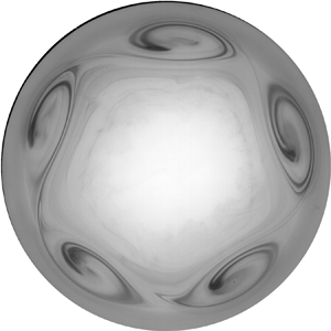
Figure 2. Instability patterns breaking the axisymmetry of the flow. Photograph taken from above (ink visualisation) in our experimental set-up. Modes $m = 3$, 4 and 5 obtained for different aspect ratios and different values of ${{\textit {Re}}}$ above the effective ${{\textit {Re}}}{}_c$; (a) $m=3$, $G=3.5/14$, ${{\textit {Re}}}=2160$, (b) $m=4$, $G=1.5/14$, ${{\textit {Re}}}=5623$, (c) $m=5$, $G=1/14$, ${{\textit {Re}}}=4714$.

2.2. Experimental technique

The main element of the experimental set-up is a cylindrical shaped Plexiglas cavity. Its internal radius is $R = 140.3 \pm 0.05$ mm, and the thickness of the Plexiglas is 6.8 mm. The value of $R$ is used to define the Reynolds number ${{\textit {Re}}}=\Omega R^{2}/\nu$. The cavity was engineered from a single block, so that the cylinder and the bottom are monolithic, preventing any risk of leak. Its bottom is drilled along its axis in order to mount a brass foot that hosts the shaft of the rotating disc, itself also made of brass. The radius of the disc is $R_d=139.6$ mm, its thickness 8.5 mm and its mass 5 kg. The shaft is held in place with two ball bearings, and the sealing is insured by a spring-loaded double-lip seal. An aluminium rigid sleeve coupling, relying on a thrust ball bearing, is used to connect the disc shaft and the motor reducer unit. The motor used is a direct current motor (Parvex RX320E-R1100) with a 1 : 12 reducer. The rotation speed is controlled using a closed-loop tachometer. Special attention was paid to minimising the gap between the disc edge and the vertical wall of the cavity. The liquids used in this experimental investigation are tap water, de-ionised water and a water–glycerol mixture. As the cavity is not thermo-regulated, the fluid temperature is monitored continuously, with a digital thermometer that allows it to be known with an accuracy of 0.1 K. The corresponding kinematic viscosity is then evaluated using an empirical formula (Cheng Reference Cheng2008). The experimental Reynolds number, based on the angular velocity $\Omega$, the radius and the kinematic viscosity are hence known within a given accuracy of the order of a per cent for the range of parameters investigated. The relative error is expected to increase as the rotation rate decreases.

Flow measurements are made using a laser Doppler velocimetry (LDV) device, composed of a Dantec Laser linked to a BSAFlow processor. The liquid is seeded with Dantec 10 micrometre diameter silver coated hollow glass spheres (S-HGS-10). These are not provided as suspension and thus prevent the introduction of additional surfactant. We also avoided to premix the particles without any additional solutant. Because of the cylindrical geometry, as the laser beams are placed for the acquisition of $u_{\theta }$ they undergo a deviation that both shifts the location of the focus and impacts the quantitative measurements. This is fixed at the post-processing stage using the technical corrections suggested in Huisman, van Gils & Sun (Reference Huisman, van Gils and Sun2012). For visualisations such as in figure 2, the flow patterns were highlighted by injecting either Kalliroscope or ink into the fluid. The protocol to find experimentally the critical Reynolds number is to progressively increase the azimuthal velocity with steps of 0.5 r.p.m. for the water and for the 20 % water–glycerol mixture, and steps of 1 r.p.m. for the 55 % water–glycerol mixture. After each increase of the rotation speed, a waiting time of 5–10 min is followed by LDV acquisition performed over another five minutes duration. This procedure allows the base flow to be almost established before the instability grows.

2.3. Experimental evidence for $m=5$ instability

We describe the experimental instability leading to a steadily rotating $m=5$ mode, using Kalliroscope visualisations or pointwise LDV measurements. The flow is initially at rest. The angular velocity is directly set to a finite value defining the target Reynolds number ${{\textit {Re}}}$, the value used in figure 3 being ${{\textit {Re}}}=16\,650$. For low enough Reynolds numbers, the flow remains axisymmetric as in figure 3(a). Above threshold, an annulus characterised by stronger shear appears around $r=0.7 R$ (figure 3b). An $m=5$ mode emerges (figure3c) and evolves towards a steadily rotating configuration with 5 co-rotating vortices (figure3d). In the time sequence presented, the Reynolds number is well above the threshold as will be seen later. In such a case, the emergence of the instability is almost concomitant with that of the base flow, which is here approximately 80 s. A similar scenario occurs for other values of $m$, in particular for $m=4$ which has been observed for other nearby values of ${{\textit {Re}}}$. The vortex pattern rotates with a constant angular velocity smaller than $\Omega$. The angular frequency $f$ of the pattern can be deduced using $f=2{\rm \pi} f_d /(m\Omega )$, where $f_d$ is the dimensional frequency obtained experimentally using pointwise LDV measurements at a location fixed in the laboratory frame. The main frequency $f$ varies moderately over the range ${{\textit {Re}}}=[4230,16\,300]$. A Fourier transform of the time series is shown in figure 4 in the case $m=5$ for ${{\textit {Re}}}=4230$ and ${{\textit {Re}}}=16\,300$. The main frequency and the related harmonics dominate the spectrum.

Figure 3. Instability growth for a $m=5$ mode for a water $+$ Kalliroscope mixture initially at rest: $G=1/14$, Reynolds number ${{\textit {Re}}}=16\,550$; (a) $t=52$ s, (b) $t=60$ s, (c) $t=71\,{\rm s}$, (d)$t=99\,{\rm s}$.

Figure 4. Experimental frequency amplitude spectrum of azimuthal velocity component measured at radius $0.76R$ and height $0.9H$ for the saturated $m=5$ regime at ${{\textit {Re}}}=4230$ and ${{\textit {Re}}}=16\,300$. The maximum amplitudes correspond to the non-dimensional frequencies $f=0.76$ and $f=0.73$, respectively.

2.4. Numerical methodology for free-slip interfaces

As a complementary part of this investigation, we have used numerical tools based on the incompressible Navier–Stokes equations in order to investigate both the linear and nonlinear aspects of the symmetry-breaking instability. The present section first introduces the numerical methods used. It also features a comparison with the experimental results of § 2.3.

2.4.1. Mathematical model

We adopt the point of view of a single-phase flow. The velocity field $\boldsymbol {u}(r,\theta ,z,t)$ inside the liquid is governed by the incompressible Navier–Stokes equations in the (non-rotating) laboratory frame

(2.1)\begin{gather} \boldsymbol{\nabla} \boldsymbol{\cdot} \boldsymbol{u} = 0, \end{gather}

(2.2)\begin{gather}\frac{\partial \boldsymbol{u}}{\partial t} + (\boldsymbol{u} \boldsymbol{\cdot} \boldsymbol{\nabla})\boldsymbol{u} = - \boldsymbol{\nabla}p + \frac{1}{{{\textit{Re}}}} {\boldsymbol\nabla}^{2}{\boldsymbol{u}}. \end{gather}

Equations (2.1)–(2.2) have been non-dimensionalised using the length scale $R$ and the time scale $\Omega ^{-1}$, and the dimensionless fluid density is taken as unity. From here on all the variables are non-dimensional except when explicitly noted.

The flow obeys no slip at all solid boundaries. This implies

(2.3)\begin{equation} u_r= u_{\theta} = u_z = 0 \end{equation}

at the fixed vertical boundary at $r=1$, whereas

(2.4a,b)\begin{equation} u_r = u_z = 0,\quad u_{\theta} = r \end{equation}

on the rotating disc at $z=0$.

The boundary condition at the liquid–gas interface at $z=G$ is classically derived from the stress balance at the interface. As the viscosity of the air is much smaller than the water one, we can neglect the gas phase altogether. We first consider the generic free-slip boundary conditions

(2.5a–c)\begin{equation} \frac{\partial u_r }{\partial z}=0,\quad \frac{\partial u_{\theta}}{\partial z}=0, \quad u_z=0 \quad \mbox{at}\ z=G. \end{equation}

A few precautions are necessary to justify the plane interface hypothesis. A numerical estimation of the height $h(r)$ as a function of the rotation speed is possible for the steady base flow. This is achieved using the variation of the numerical code ROSE with coordinate transformations used in Yang et al. (Reference Yang, Delbende, Fraigneau and Martin Witkowski2020). Two sets of parameters typical of the present range of interest have been considered. The first set is a least favourable parameter case ($G=1/14$, $\Omega = 0.95\,\textrm {rad}~\textrm {s}^{-1}$), i.e. ${{\textit {Re}}} = 18\,620$ and $Fr=(\Omega ^{2} R)/g=0.013$ where $g$ is the gravity. In this case, the total height variation from the centre to the periphery is ${\rm \Delta} h=h(r=1)-h(r=0)=6.8\,\%$ of the undisturbed fluid height. The second set is for the rotation rate at which the instability is first detected (${{\textit {Re}}} \sim 3000$), $\Omega =0.15$ rad s$^{-1}$ and $Fr=3.34\times 10^{-4}$, ${\rm \Delta} h$ is less than 0.2 %. Such small values, respectively 0.68 and 0.017 mm (too small to be measured experimentally for the latter), justify the flat interface hypothesis considered in the numerical part.

As in all mesh-based numerical methods, the singularities of the velocity field occurring at both corners $(r=1,z=0)$ and $(r=1,z=G)$ are smoothed out in practice by the finite mesh without the need, as for spectral methods, for regularising functions (Serre & Bontoux Reference Serre and Bontoux2007) or singular splitting (Duguet, Scott & Le Penven Reference Duguet, Scott and Le Penven2005). This is consistent with the ‘natural’ regularisation occurring in the experiment in the presence of a very thin gap.

2.4.2. Linear stability analysis

In order to determine the critical Reynolds number ${{\textit {Re}}}{}_c$ for the onset of instability, we use an in-house linear stability solver named ROSE, based on a finite difference method in $r$ and $z$. The technique as well as the equations written in cylindrical coordinates are found in Kahouadji, Houchens & Martin Witkowski (Reference Kahouadji, Houchens and Martin Witkowski2011). The steady axisymmetric base flow is first determined by solving (2.1) and (2.2) together with the associated boundary conditions using a Newton–Raphson solver. The steady solution is solved for in an $(\omega , \psi , u_\theta , c)$ formulation, where

(2.6a–c)\begin{equation} \omega = \frac{\partial u_r}{\partial z} - \frac{\partial u_z}{\partial r},\quad u_r = \frac{1}{r} \frac{\partial \psi}{\partial z}, \quad u_z = -\frac{1}{r} \frac{\partial \psi}{\partial r}. \end{equation}

The Newton–Raphson solver allows for additional scalar fields $c(r,z)$ such as temperature or concentration, as further discussed in § 4.

Let $(\boldsymbol {U},P)$ represent the velocity-pressure field for such a steady axisymmetric solution of (2.2), and let $(\boldsymbol {u}^{*},p^{*})$ be a small-amplitude perturbation to $(\boldsymbol {U},P)$. The dynamics of the perturbation is governed by the linearised stability equations

(2.7)\begin{gather} \boldsymbol{\nabla} \boldsymbol{\cdot} \boldsymbol{u}^{*} = 0, \end{gather}

(2.8)\begin{gather}\frac{\partial \boldsymbol{u}^{*} }{\partial t} + (\boldsymbol{U} \boldsymbol{\cdot} \boldsymbol{\nabla})\boldsymbol{u}^{*} + (\boldsymbol{u}^{*} \boldsymbol{\cdot} \boldsymbol{\nabla})\boldsymbol{U} = - \boldsymbol{\nabla}p^{*} + \frac{1}{{{\textit{Re}}}} {\boldsymbol\nabla}^{2}{\boldsymbol{u}^{*}}. \end{gather}

It is associated with Dirichlet boundary conditions $\boldsymbol {u}^{*}=0$ on all solid boundaries together with a boundary condition on $\boldsymbol {u}^{*}$ at the interface similar to that for $\boldsymbol {u}$ in (2.5). The velocity field and the pressure field are decomposed using a complex ansatz of the form $\textrm {e}^{\lambda t+\textrm {i}\,m\theta }$, as will be detailed in § 4.2. The neutral curve corresponds to parameter values where the real part ${\textrm {Re}}(\lambda )=0$, and it is identified in practice using a one-dimensional secant method. All meshes used are Cartesian in the meridional plane $(O,\boldsymbol {r},\boldsymbol {z})$. For $G=1/14$ the mesh consists of $701\times 101$ grid points.

2.4.3. Direct numerical simulation

For the nonlinear validation of the stability thresholds we have used the direct numerical simulation (DNS) code Sunfluidh developed at LIMSI for incompressible flows. It is based on a projection method to ensure a divergence-free velocity field. The equations are discretised on a staggered structured non-uniform grid using a finite volume approach with a second-order centred scheme in space. A second-order backward Euler differentiation is used for time discretisation. Details can be found in Yang et al. (Reference Yang, Delbende, Fraigneau and Martin Witkowski2020). The interface condition is as in (2.3) and (2.4). The code offers the possibility to enforce a given rotational symmetry $\mathcal {R}_m$ characterised by a fundamental azimuthal wavenumber $m\ge 0$, such that every velocity field verifies

(2.9)\begin{equation} (\mathcal{R}_m{\boldsymbol{u}})(r,\theta,z)={\boldsymbol{u}}\left(r,\theta+\frac{2{\rm \pi}}{m},z\right)={\boldsymbol{u}}(r,\theta,z)\quad (m \neq 0), \end{equation}

or axisymmetry for $m=0$. If $m \neq 0$ the simulation only needs to be carried out over an angular sector $0\le \theta \le 2{\rm \pi} /m$ with azimuthal periodicity. For the simulations without symmetry imposed, we have used a mesh consisting of $180\times 180\times 64$ cells in $r$, $\theta$ and $z$, respectively.

3.1. Comparison between the numerical methods

For identical parameters, we report excellent agreement between the base flows computed by the two methods for all ${{\textit {Re}}}$. Whereas the base flow can be converged for all ${{\textit {Re}}}$ using the Newton method, it is only accessible for ${{\textit {Re}}}<{{\textit {Re}}}{}_c$ using time stepping. However, since the base flow is apparently the only axisymmetric solution of the system, it is also found using DNS for all ${{\textit {Re}}}$ by simply imposing $m=0$ (two-dimensional axisymmetric case) and stepping forward in time. The value of ${{\textit {Re}}}{}_c$ for $m=5$ is first identified by LSA using a secant method. In the DNS code, the procedure used to identify ${{\textit {Re}}}{}_c$ is different; above and below ${{\textit {Re}}}{}_c$, an arbitrary perturbation of finite but small amplitude is applied to the system after an initial transient, with the $\mathcal {R}_5$ symmetry imposed or not. This impulse response leads to either exponential decay towards the base flow, or exponential growth towards a nonlinear regime at large times. A linear interpolation of these rates leads to an evaluation of the critical threshold ${{\textit {Re}}}{}_c$. Both approaches agree quantitatively very well regarding the prediction of ${{\textit {Re}}}{}_c$ for $m=5$ since the relative error is close to 0.3 % (see table 1). Interestingly, this comparison, as well as the lack of unstable impulse response for ${{\textit {Re}}}<{{\textit {Re}}}{}_c$ (even for larger-amplitude impulses), both suggest that the instability is supercritical and not subcritical, at least for a clean interface obeying the boundary condition (2.5). Note that the ROSE computation in table 1 was performed using a $701 \times 101$ grid. Numerical comparison with Kahouadji et al. (Reference Kahouadji, Martin Witkowski and Le Quéré2010) confirms that this resolution is sufficient for an estimation of ${{\textit {Re}}}{}_c$ with an accuracy of less than one per cent. Two additional computations were performed using different meshes. The ${{\textit {Re}}}{}_c$ was estimated to 17 032 with a $351 \times 51$ grid, and to 16 992 with a $1401 \times 201$ grid. The maximum variation of ${{\textit {Re}}}{}_c$ is less than 0.16 % compared to the value in table 1.

3.2. Mean flow structure

Since both numerical approaches yield a truly similar base flow solution, a comparison with the experimental base flow measured using LDV would be relevant at this point. As we shall see, measurements below ${{\textit {Re}}}{}_c$ turn out to be experimentally difficult. Another comparison, which is easier to perform, concerns the mean velocity profiles obtained for ${{\textit {Re}}}>~{{\textit {Re}}}{}_c$ by either temporal or spatial average. Such a comparison is displayed in figure 5. For the eigenmodes computed using ROSE, their average is by construction zero. Hence, only the base flow obtained by LSA is included in figure 5, whereas the spatial average is taken for the DNS data and the time average for experimental LDV data. A common value of ${{\textit {Re}}}=18\,620$ is chosen for the comparison. Although the agreement is satisfactory, a noticeable overshoot appears around $r \approx 0.67$ in all numerical azimuthal velocity profiles, with no equivalent in LDV measurements despite sufficient measurement accuracy. The same mismatch, presence of the overshoot area in numerics, but not in experiments, was also reported for comparable parameters in Yang et al. (Reference Yang, Delbende, Fraigneau and Martin Witkowski2019). The computations performed on different meshes all display this overshoot, which rules out a numerical artefact.

Figure 5. Velocity profiles of $u_{\theta }(r)$ below the free surface ($z=0.8G$) for $G=1/14$ and ${{\textit {Re}}}=18\,620$. Comparison between the base flow, spatially averaged DNS and the temporal average for LDV (experiment). LDV acquisition timespan is much larger than the instability period.

3.3. Threshold detection

The most dramatic mismatch between numerics and experiments concerns the critical Reynolds number. While both numerical simulations agree on a critical Reynolds number of approximately $17\,000$ (see table 1), LDV measurements display persistent oscillations in the azimuthal velocity field for ${{\textit {Re}}}$ as low as $4200$, with a normalised frequency $f_5=0.76$, indicative of the presence of the $m=5$ mode. This upper bound on the value of ${{\textit {Re}}}{}_c$ is smaller by a factor of 4 than the previous experimental estimates by Poncet & Chauve (Reference Poncet and Chauve2007). These values can be found in table 1. The discrepancies are robust; although the exact same spin-up protocol as Poncet & Chauve (Reference Poncet and Chauve2007) was observed, the respective ranges of ${{\textit {Re}}}{}_c$ differ. We note that the threshold detection by Poncet & Chauve (Reference Poncet and Chauve2007) is based on Kalliroscope visualisations. Kalliroscope appears in our set-up as a poor diagnostic for ${{\textit {Re}}}{}_c$ for this flow case; the threshold detection is erratic and protocol dependent. Indeed the estimation of ${{\textit {Re}}}{}_c$ fluctuates between 6200 to 9300. At times, Kalliroscope is even unable to detect the instability, even well above the value of ${{\textit {Re}}}{}_c$ predicted numerically. The use of ink for visualisation, and LDV for quantitative measurements, both confirm that the thresholds detected with Kalliroscope are over-evaluated. The saturated mode is displayed in figure 2 at a value of ${{\textit {Re}}}$ approximately 4 times lower than the theoretical threshold ${{\textit {Re}}}{}_c^{(LSA)}$. Its spatial structure is directly comparable to that of the saturated flow above ${{\textit {Re}}}{}_c^{(LSA)}$ displayed in figure 3(d).

On the one hand, there is perfect numerical agreement between LSA and DNS about the estimation of ${{\textit {Re}}}{}_c$, on the other hand, there is a troubling match with Poncet & Chauve (Reference Poncet and Chauve2007) at odds with the experimental/numerical discrepancy we report. We have hence carried out an exhaustive investigation of the possible reasons for such a discrepancy by focusing on experimental imperfections. A classical reason for discrepancies in rotating machines is the presence of mechanical noise that could force an instability by direct or parametric resonance. The experimental displacement of the disc surface was measured using a pair of LK-G10 sensors, and their associated LK-GD500 controller. Displacements were evaluated to approximately $10^{-4}$ m, with a mean frequency corresponding to the disc rotation, yet no link with the pattern frequency was found. This does not suggest any obvious experimental flaw in our experimental methodology.

Eventually, in order to confirm our experimental approach, we switch temporarily to a different geometry with $G=1/4$ where a direct and favourable comparison with the experimental results of Lopez et al. (Reference Lopez, Marques, Hirsa and Miraghaie2004) can be made. For these parameters there is also a robust mismatch between experiments and numerics; LSA predicts the most unstable mode $m=2$ with ${{\textit {Re}}}{}_c=3500$, whereas Lopez's experiments at ${{\textit {Re}}}=2000$ show a mode $m=3$, predicted using LSA to be unstable only for ${{\textit {Re}}} \geq 4600$. We have then conducted our own experiments with two different mixtures of water with $20\,\%$ and $55\,\%$ glycerol. The motivation for these two different mixtures is to allow for a wider span of rotation speeds; using water the instability would have occurred for rotation speed below 1 r.p.m. where the signal-to-noise ratio in the LDV degrades. In both cases the mode $m=3$ is detected, either using ink or LDV, for ${{\textit {Re}}}=2160$ in the $55\,\%$ glycerol fluid (see figure 2a) and ${{\textit {Re}}}=2520$ in the $20\,\%$ glycerol fluid. All the results are gathered in table 2. This side study confirms, in good agreement with Lopez et al. (Reference Lopez, Marques, Hirsa and Miraghaie2004) that numerics overestimate the experimental thresholds in ${{\textit {Re}}}$. The discrepancy reported here for $G=1/14$ has hence a robust physical origin, which the rest of this paper is devoted to.

Table 2. Critical Reynolds number for $G=1/4$. Comparison between experiments by Lopez et al. (Reference Lopez, Marques, Hirsa and Miraghaie2004), present experiments and LSA. The percentage of glycerol indicated is a weight percentage.

3.4. Nonlinear dynamics

The mismatch between numerics and experiments for $G=1/14$ is even more dramatic further above ${{\textit {Re}}}{}_c$. Although DNS initially displays an azimuthal wavenumber $m=5$ close to ${{\textit {Re}}}{}_c$ (see figure 6a at ${{\textit {Re}}}=17\,100$), the instability pattern evolves towards $m=7$ as ${{\textit {Re}}}$ is pushed to 18 620, less than 9 % above ${{\textit {Re}}}{}_c$. Poncet & Chauve (Reference Poncet and Chauve2007) have also reported an evolution of the modal content of the flow with ${{\textit {Re}}}$, yet with $m$ decreasing as ${{\textit {Re}}}$ is increased. A similar decrease of $m$ with ${{\textit {Re}}}$ was also observed qualitatively in our experiment for ${{\textit {Re}}}$ sufficiently higher than ${{\textit {Re}}}{}_c$. However, the wavenumber $m=5$ remains experimentally stable from ${{\textit {Re}}}=4200$ to at least ${{\textit {Re}}}=18\,620$. The frequency spectrum is shown in figure 7(a) for ${{\textit {Re}}}=18\,620$. Given such a mismatch, larger values of ${{\textit {Re}}}$ were not investigated, neither experimentally nor numerically. Differences in the nonlinear dynamics for ${{\textit {Re}}}=18\,620$ also emerge in velocity measurements; while experimental time series display a single frequency, the signals from DNS display a broader spectrum and richer dynamics, see figure 7. In addition to the mismatch in the modal behaviour between experiments and DNS, the vorticity patterns (figures 6a and 6b) do not match the experimental (figures 2 and 3d) very convincingly. This raises doubts about whether the mode predicted in the numerics does indeed correspond to the structure observed experimentally.

Figure 6. DNS axial vorticity fluctuation for the free-surface condition, ${{\textit {Re}}}=17\,100$ slightly above ${{\textit {Re}}}{}_c$ (a), and ${{\textit {Re}}}=18\,620$ (b). With the increase of ${{\textit {Re}}}$, the mode $m=5$ selected at ${{\textit {Re}}}{}_c$ evolves into a modulated $m=7$ pattern.

Figure 7. Comparison of frequency amplitude spectra for $u_{\theta }(t)$ measured at $r=0.76$, $z=0.8G$, for the saturated $m=5$ regime at ${{\textit {Re}}}=18\,620$. (a) Experimental data, maximum peak at $f=4.15$. (b) DNS with free-surface condition, same parameters. The frequencies are not normalised by the azimuthal wavenumber.

3.5. Limitations of the clean interface hypothesis

Lopez et al. (Reference Lopez, Marques, Hirsa and Miraghaie2004) have suggested that mismatches in critical Reynolds numbers between theoretical and experimental predictions arise due to the presence of pollutants at the interface. The main idea is that the pollutants change the boundary condition at the interface. One can draw a parallel with the evolution from free slip to no slip examined by Peaudecerf et al. (Reference Peaudecerf, Landel, Goldstein and Luzzatto-Fegiz2017) in a channel flow with superhydrophobic surfaces, in presence of carefully added surfactants. As it is nearly impossible, in standard laboratory conditions, to achieve an experiment with a perfectly clean interface at all times, it is necessary to take additional effects into account in order to properly model the behaviour of the fluid at a realistic liquid–gas interface. Previous publications with a similar experimental set-up, in which the adsorption of pollutants at the interface was carefully controlled, already demonstrated the crucial influence of pollution of the base flow (Hirsa et al. Reference Hirsa, Lopez and Miraghaie2001; Hirsa, Lopez & Miraghaie Reference Hirsa, Lopez and Miraghaie2002a). There, pollutants were assimilated to a monolayer of vitamin $K1$, considered as a surfactant, yet any insoluble (or weakly soluble) surfactant would have a similar effect.

In the next section, we model explicitly the presence of pollutants at the interface in the Navier–Stokes equations and investigate its qualitative as well as quantitative influence on the linear stability of the flow.

4.1. Modification of the effective surface tension

The present modelling of the pollution at the interface is directly inspired by the modelling in Hirsa et al. (Reference Hirsa, Lopez and Miraghaie2001) and Kwan, Park & Shen (Reference Kwan, Park and Shen2010). Let $c_d(r, \theta , t)$ be the dimensional instantaneous concentration of the pollutants at the interface, the closure equation between the surface tension $\sigma$ and $c_d$ reads

(4.1)\begin{equation} \sigma=\sigma_0\left(1-\frac{\alpha}{2 \sigma_0}c_d^{2}\right), \end{equation}

where $\sigma _0$ is the reference surface tension of the solvent (for water, $\sigma _0=72.8~\textrm {mN}~\textrm {m}^{-1}$); $\alpha$ is a dimensional constant coming from the Taylor expansion around $c_d=0$ of the model in Kwan et al. (Reference Kwan, Park and Shen2010), and depends from the chemical species of the pollutant. Equation (4.1) is non-dimensionalised as

(4.2)\begin{equation} \bar{\sigma}=1-\frac{\alpha C_0^{2}}{2 \sigma_0}{c}^{2}, \end{equation}

where $\bar {\sigma }=\sigma /\sigma _0$ and $c = c_d/C_0$. Here, $C_0$ represents the average mass concentration of pollutant at the interface, such as

(4.3)\begin{equation} C_0 = \frac{1}{{\rm \pi} R^{2}} \int_0^{2{\rm \pi}}\int_{0}^{R} {c_d}(r,\theta,t) r\,{\textrm{d}}r\,{\textrm{d}}\theta. \end{equation}

Since the ambient pollution is undetermined, the value of the $\alpha$ coefficient is unknown. Thus (4.2) is modified as follows

(4.4)\begin{equation} \bar{\sigma}=1-\frac{\beta {{\textit{Ca}}}}{2}{c}^{2}, \end{equation}

where ${{\textit {Ca}}} =\mu \Omega R/\sigma _0$ is a capillary number, $\mu$ is the dynamic viscosity and $\beta$ is a new non-dimensional control parameter defined by

(4.5)\begin{equation} \beta = \frac{\alpha C_0^{2}}{\mu \Omega R }. \end{equation}

Note that $\beta$ can be linked to a Marangoni number, based on $C_0$ and the diffusion $D^{s}$ such that ${{\textit {Ma}}} = (\alpha C_0^{2} R)/(D^{s} \mu )$, and to the Péclet number ${{\textit {Pe}}}^{s} =\Omega R^{2}/D^{s}$ so that $\beta = {{\textit {Ma}}}/{{\textit {Pe}}}^{s}$.

We assume that pollutants are advected by the velocity field of the fluid while diffusing with a simple non-dimensional diffusion coefficient $D^{s}$. Moreover, we assume that no transport occurs from the surface to the bulk of the flow, so that the bulk concentration can be neglected (Bandi et al. Reference Bandi, Akella, Singh, Singh and Mandre2017). In practice, $\beta$ is limited by chemistry considerations; high values of $\beta$ correspond to a highly polluted surface. Under these conditions, diffusion into the bulk becomes possible. Starting from the Boussinesq–Scriven surface fluid model for a Newtonian fluid–gas interface (Scriven Reference Scriven1960), and under the hypothesis of negligible surface dilatational viscosity and surface shear viscosity (Hirsa et al. Reference Hirsa, Lopez and Miraghaie2001), the boundary conditions can be written as

(4.6a–c)\begin{equation} \frac{\partial u_r}{\partial z} = \frac{1}{{{\textit{Ca}}}}\frac{\partial \bar{\sigma}}{\partial r},\quad \frac{\partial u_{\theta}}{\partial z} = \frac{1}{{{\textit{Ca}}}}\frac{1}{r}\frac{\partial \bar{\sigma}}{\partial \theta},\quad u_z=0. \end{equation}

Using (4.4) and the expression of $\beta$, (4.6) can hence be rewritten

(4.7a–c)\begin{equation} \frac{\partial u_r}{\partial z} = -\beta c \frac{\partial {c}}{\partial r}, \quad \frac{\partial u_{\theta}}{\partial z} = -\beta c \frac{1}{r}\frac{\partial {c}}{\partial \theta}, \quad u_z=0. \end{equation}

The introduction of $\beta$ allows for a simpler study since it is the only input parameter for the LSA.

4.2. Modelling of pollutant concentration

When all pollutants stay at the interface $z=G$, their concentration $c(r,\theta ,t)$ obeys a superficial advection–diffusion equation of the form

(4.8)\begin{equation} \frac{\partial c}{\partial t} + \boldsymbol{\nabla}^{s} \boldsymbol{\cdot} (c \boldsymbol{u^{s}})+c(\boldsymbol{\nabla}^{s} \boldsymbol{\cdot} \boldsymbol{n}) (\boldsymbol{u} \boldsymbol{\cdot} \boldsymbol{n}) = \frac{1}{{{\textit{Pe}}}^{s}} {{\rm \Delta}^{s}} c, \end{equation}

where $\boldsymbol {\nabla }^{s}$ represents the gradient operator in the directions tangent to the interface, $\boldsymbol {\nabla }^{s}$ represents the gradient operator in the directions tangent to the interface and ${\rm \Delta} ^{s}$ is the associated Laplacian (Stone Reference Stone1990). In (4.8), the original velocity field $\boldsymbol {u}$ is split into a normal component $(\boldsymbol {u} \boldsymbol {\cdot } \boldsymbol {n})\boldsymbol {n}$ and the resulting tangential component $\boldsymbol {u^{s}}=\boldsymbol {u}-(\boldsymbol {u} \boldsymbol {\cdot } \boldsymbol {n})\boldsymbol {n}$. In the simple case where $\boldsymbol {n}=\boldsymbol {e_z}$, (4.8) reduces to

(4.9)\begin{equation} \frac{\partial c}{\partial t} + \boldsymbol{\nabla}^{s} \boldsymbol{\cdot} (c \boldsymbol{u^{s}}) = \frac{1}{{{\textit{Pe}}}^{s}} {\rm \Delta}^{s} c. \end{equation}

We consider a decomposition into base flow and perturbation, where the perturbation is written using a complex ansatz of the form $\textrm {e}^{\lambda t + \textrm {i}\,m\theta }$, such that $u_r=U_r+u_r^{*} \,\textrm {e}^{\lambda t + \textrm {i}\,m \theta }$, $u_{\theta }=U_{\theta }+ \textrm {i}\, u_{\theta }^{*} \,\textrm {e}^{\lambda t + \textrm {i}\,m\theta }$ and $c=C+c^{*} \,\textrm {e}^{\lambda t + \textrm {i}\,m\theta }$. For the steady axisymmetric base flow characterised by the velocity field $\boldsymbol{ U}$ and the concentration field $C$, (4.9) becomes

(4.10)\begin{equation} \frac{1}{r}\frac{\partial{rCU^{s}_r}}{\partial r} - \frac{1}{{{\textit{Pe}}}^{s}} \left(\frac{\partial{{}^{2} C}}{\partial r^{2}}+\frac{1}{r}\frac{\partial{C}}{\partial r} \right)=0. \end{equation}

By subtracting (4.10) from (4.9), the equation for the disturbance concentration $({\boldsymbol {u}},c)$ reads

(4.11)\begin{align} -\lambda c^{*} = \frac{1}{r} \left(\frac{\partial{rC {u}_r^{*}}}{\partial r} + \frac{\partial{rU_r c^{*}}}{\partial r}\right)+\frac{\textrm{i}\,m U_{\theta} c^{*}}{r}-\frac{mC u_{\theta}^{*}}{r} -\frac{1}{{{\textit{Pe}}}^{s}}\left(\frac{\partial{{}^{2} c^{*}}}{\partial r^{2}}+\frac{1}{r}\frac{\partial{c^{*}}}{\partial r}-\frac{m^{2} c^{*}}{r^{2}}\right). \end{align}

The diffusion coefficient $D^{s}$ for the pollutants is usually one or two orders of magnitude smaller than the kinematic viscosity and thus, in the present case, superficial diffusion effects remain small with respect to advection effects.

The constraint (4.3) reads in non-dimensional form

(4.12)\begin{equation} \frac{1}{\rm \pi} \int_0^{2{\rm \pi}}\int_{0}^{1} {c}(r,\theta,t)r\,{\textrm{d}}r\,{\textrm{d}}\theta= 1, \end{equation}

and reduces for the steady axisymmetric base flow to

(4.13)\begin{equation} 2 \int_{0}^{1} {C}(r)r\,{\textrm{d}}r = 1. \end{equation}

For the base flow, axisymmetry implies ${\partial C}/{\partial r}=0$ at the axis. The constraint (4.13) also imposes a zero mass flux at $r=1$. For the perturbation field $c^{*}$, the boundary conditions depend on the value of the azimuthal wavenumber $m$ (Kahouadji et al. Reference Kahouadji, Houchens and Martin Witkowski2011). For $m \geq 1$ (the case of interest), $c^{*}=0$ is imposed at the axis and ${\partial c^{*}}/{\partial r}=0$ at the outer wall. All superscripts $^{*}$ are from here on dropped for simplicity.

4.3. Structure of the modified base flow

As demonstrated in Lopez & Chen (Reference Lopez and Chen1998), the presence of a surfactant layer at the interface modifies the structure of the base flow. However, the potential influence on its linear stability has not been investigated yet. In this subsection, we study the influence of the pollution concentration $\beta$, modelled using the surfactant law (4.1), on the base flow for $G=1/14$ and ${{\textit {Re}}}=18\,620$. Increasing $\beta$ causes a small but monotonic decrease of the length of the meridional recirculation, see figure 8. This is accompanied by the progressive disappearance of the overshoot in $U_{\theta }$, evident in figure 9. This observation is directly consistent with the experimental measurements, in which no overshoot has been found for $z=0.8G$.

Figure 8. Evolution of the streamfunction $\psi$ for the base flow with increasing concentration $\beta$, ${{\textit {Re}}}=18\,620$ and $G=1/14$. The same contour values are chosen for all cases. Negatives and positives contours use different scales to highlight the weak recirculation bubble. Negatives contour values (dashed): four equispaced levels in [$\psi _{min} - \psi _{min}/5$]. Positives contour values: (solid lines): nine values equispaced levels in [$\psi _{max}/10 - \psi _{max}$]. Zero contour level (solid black lines). $\psi _{min} = -8.1 \times 10^{-5}$ and $\psi _{max} = 2.3 \times 10^{-3}$; (a) $\beta =0$, (b) $\beta =0.1$, (c) $\beta =0.2$, (d) $\beta =0.5$.

Figure 9. Evolution of the azimuthal velocity $U_{\theta }$ for the base flow for increasing $\beta$, ${{\textit {Re}}}=18\,620$ and $G=1/14$. 21 equispaced levels in [0–1]. Translucent red patches represent overshoot areas, i.e. locations where $U_{\theta } \ge 1.01\,r$; (a) $\beta =0$, (b) $\beta =0.1$, (c) $\beta =0.2$, (d) $\beta =0.5$.

4.4. Linear instability thresholds for $G=1/14$

The present model is based on four independent non-dimensional parameters $G$, ${{\textit {Re}}}$, ${{\textit {Pe}}}^{s}$ and $\beta$. We have investigated quantitatively the influence of $\beta$ on the instability thresholds ${{\textit {Re}}}{}_c$ for $m=4$ and 5, with $G$ fixed to 1/14 except when noted. The numerical resolution is unchanged compared to the pollution-free case. The Péclet number, although in principle larger, is hence limited to ${{\textit {Pe}}}=10^{3}$ in order to prevent steeper gradients and numerical issues. The focus on $m=4$ and 5 mirrors the modal selection predicted for the reference case $\beta =0$, and is also consistent with experimental findings at onset.

The neutral curves ${{\textit {Re}}}{}_c(\beta )$ obtained as $\beta$ is varied are shown in figure 10, where neutral modes $m=4$ and 5 appear as squares and five-pointed stars, respectively. The neutral curves have been determined by identifying the parameters where ${\textrm {Re}}({\lambda })=0$ using a secant method. In some intervals of $\beta$ the curve ${{\textit {Re}}}{}_c(\beta )$ happens to be multi-valued, see e.g. $\beta =0.3$ for $m=4$; several thresholds can be found for this value of $\beta$, although no trivial physical interpretation has been found. In such cases, the code was modified to determine the critical value of $\beta$ for a given value of ${{\textit {Re}}}$. Note that the influence of the numerical resolution on ${{\textit {Re}}}{}_c$ for $\beta =5$ has been verified using the same numerical grids as for $\beta =0$ ($351 \times 51$ and $1401 \times 201$), with variations below 0.58 %.

Figure 10. Neutral curve ${{\textit {Re}}}_c(\beta )$ estimated from LSA for $G=1/14$ and for the modes $m=4$ (squares) and $m=5$ (stars). The blue stripe corresponds to the experimental value of ${{\textit {Re}}}{}_c$, independent of the model based on $\beta$. The thickness of the stripe is based on lower and upper bounds for ${{\textit {Re}}}{}_c$ from table 1. The inset figure represents in semi-log coordinates the continuation of the curves for $\beta \in$ [3:100].

The most striking result in figure 10 is the dramatic drop in ${{\textit {Re}}}_c$ occurring at $\beta \approx 0.48$ for $m=4$ and $\beta \approx 0.14$ for $m=5$. The asymptotic value of ${{\textit {Re}}}{}_c$ predicted for large $\beta$ and approached for $\beta$ as small as 0.2, is also below $3000$ in much closer agreement with experimental estimations (shown as the blue stripe in figure 10) than the numerical prediction with $\beta =0$. These results suggest that a minute amount of surfactants can dramatically impact the flow stability, while additional pollution does not worsen the phenomenon further. In other words the effect of pollution is almost binary; either the interface is perfectly clean and the stability of the flow obeys the classical prediction from § 3, or it is not and the stability characteristics of the flow are of a fully different kind. This scenario is consistent with the experimental reproducibility of ${{\textit {Re}}}{}_c$.

For the mode $m=5$, a sharp change of slope is evident for ${{\textit {Re}}}{}_c=17\,259$, $\beta =0.14$. This marks the presence of a codimension-two point, where two different marginal curves for two different modes $m=5$ intersect in a double Hopf bifurcation; on each side of the corresponding value of $\beta$, these are not the same family of eigenmodes that go unstable first, despite a common azimuthal wavenumber $m$. The crossing of eigenvalues is confirmed in figure 11 where the pair of eigenvalues is displayed on each side of the crossing. In each case, the branch taking over for larger $\beta$ does apparently not extend down to $\beta =0$; it corresponds to a new instability not found in the clean interface case. The computation of the branches beyond the codimension-two point was performed by a restriction of the number of eigenvalues computed around a shift. This shift was set equal to the angular frequency of the most unstable eigenvalue for the previous couple of parameters (${{\textit {Re}}}{}_c$, $\beta$). The evolution of the two leading eigenvalues as functions of both $\beta$ and ${{\textit {Re}}}$ is detailed in figure 12(a). The least stable eigenvalue for the ‘clean’ case $\beta =0$ is labelled ‘$C_m$’, where $m=5$, whereas the least stable eigenvalue for the ‘dirty’ case $\beta \gg 1$ is simply labelled ‘$D_m$’. From figure 12(a) it appears that the trajectories of the eigenvalues $C_5$ and $D_5$ in the complex plane, for variations of ${{\textit {Re}}}$ and $\beta$, follow different routes; $C_5$ becomes destabilised by increasing ${{\textit {Re}}}$ but stabilised by increasing $\beta$, whereas $D_5$ is destabilised by both increasing $\beta$ and increasing ${{\textit {Re}}}$.

Figure 11. Zoom on codimension-two points of figure 10 in the ($\beta$, ${{\textit {Re}}}{}_c$) plane, for $G=1/14$, $m=4$ and $m=5$.

Figure 12. Evolution of the eigenvalues associated with the most dangerous modes (‘clean’ mode C and ‘dirty’ mode D) as a function of ${{\textit {Re}}}$ and $\beta$ for $G=1/14$; (a) $m=5$ and (b) $m=4$. The two evolutions start at ${{\textit {Re}}}=15\,000$ and $\beta =0$. The C and D eigenvalues follow the lines indicated by the red arrows as ${{\textit {Re}}}$ is increased from $15\,000$ to $17\,200$ while $\beta =0$. The eigenvalues evolve with varying $\beta$ (at constant ${{\textit {Re}}}=15\,000$, blue arrows) with equally spaced steps from 0 to 0.18 for $m=5$, and from 0 to 0.5 for $m=4$.

In the case $m=4$, an equivalent codimension-two point can be identified in figures 10 and 11, at ${{\textit {Re}}}{}_c=18\,869$, $\beta =0.17$. For this mode, the drop in ${{\textit {Re}}}{}_c$ is more dramatic than for $m=5$, and does not occur immediately after the codimension-two point. Instead, the new branch (in green in figure 10) continues to increase until at ${{\textit {Re}}}{}_c=20\,951$, $\beta =0.48$ where it turns back. Again the trajectory of the corresponding eigenvalues $C_4$ and $D_4$ is documented in figure 12(b). The trajectories of $C_4$ in the complex plane are similar to those of $C_5$. However, the scenario for $D_4$ differs from that for $D_5$; an increase in ${{\textit {Re}}}$ stabilises the corresponding eigenmode whereas an increase in $\beta$ destabilises it.

Interestingly, the asymptotic value of ${{\textit {Re}}}{}_c$ for $m=4$ as well as the corresponding value of $\beta$ at which the lowest values of ${{\textit {Re}}}{}_c(\beta )$ are reached, seem to match that for $m=5$. This suggests that the value of ${{\textit {Re}}}{}_c$ does not, for large $\beta$, depend on the value of $m$, at least for this value of $G$. Preliminary computations for $G=1/4$ have not confirmed this observation. A parametric study of ${{\textit {Re}}}{}_c$ as a function of both $G$ and $m$ would shed light on this question, but this lies outside the present scope.

The evolution of the angular frequency of the pattern at ${{\textit {Re}}}={{\textit {Re}}}_c$ is displayed in figure13 for both $m=4$ and 5 as $\beta$ is varied. Direct comparison of this figure with figure 10 shows that each jump to a new branch corresponds to a discontinuity in angular frequency. Again, the quantitative match with the experimental angular frequency is much more satisfying at finite $\beta$ than around $\beta =0$. For large $\beta$, the data approach the blue stripe in figure 13 within 1 % or less.

Figure 13. Angular frequency of the pattern $-{\rm Im}(\lambda )/m$ at ${{\textit {Re}}}={{\textit {Re}}}{}_c(\beta )$ for $G=1/14$, obtained using LSA for the modes $m=4$ (squares) and $m=5$ (stars). The blue line corresponds to the experimental value obtained using LDV (cf. table 1). The inset figure represents in semi-log coordinates the continuation of the curves for $\beta \in [3:100]$.

Visualisations in physical space of the different modal families for a common wavenumber $m$ are displayed in figure 14. From figures 10 and 13 it is now clear that these two eigenmodes correspond to two different modal families. For the $\beta =0$ case the marginal eigenmode corresponds to the one found in Kahouadji et al. (Reference Kahouadji, Houchens and Martin Witkowski2011).

Figure 14. Vorticity $\omega _z(r,\theta )$ at the fluid interface (normalised by its maximum) for the least stable eigenmode $m=5$ at ${{\textit {Re}}}=18\,620$; (a) $\beta =0$, (b) $\beta =5$.

Closer to the codimension-two point, the representation of $\omega _z$ as in figure 14 does not highlight the discrepancies between the two modes. However, the differences between them stand out again when representing the perturbation kinetic energy in a meridional plane (cf. figure 15); for the dirty mode the kinetic energy is much more localised close to $r \approx 0.7$ than for the clean mode. As for the eigenfrequencies, the variations in angular frequency are less dramatic than those in ${{\textit {Re}}}{}_c$, nevertheless angular frequencies predicted for large $\beta$ are in much better agreement with experimental values than the ones predicted for $\beta =0$.

Figure 15. Meridional sections of local kinetic energy of the eigenmodes (normalised by its maximum) for the clean branch (a) and the dirty branch (b) at the codimension-two point (${{\textit {Re}}}=17\,259$, $\beta =0.14$). The ten isolines are equispaced between 0 (dark blue) and 1 (bright yellow).

In order to evaluate the amount of pollution needed to switch from one family of branches to another, owing to (4.4), it is possible to estimate the variation of the surface tension at some point on the neutral curve. For instance, at onset $\beta =1$, ${{\textit {Re}}}{}_c=2241$ (see figure 10), the non-dimensional concentration variation for $C$ is O(1), consistently with the finding in figure 16(c) (even if the value of ${{\textit {Re}}}$ is smaller, the concentration jump is the same. The main effect of decreasing ${{\textit {Re}}}$ is to soften the slope). Equation (4.4) reduces to $\bar {\sigma }=1 - {\textit {Ca}}$ so that the capillary number is now a direct measure of the variation of surface tension. For the regime of interest with water, ${\textit {Ca}}= 10^{-3}$, so that the surface tension varies by less than 1 %, which is indeed small and nevertheless leads to a large change in $\textit{Re}_c$.

Figure 16. Comparison of several fields of the base flow at the interface, for a few values of $\beta$, at ${{\textit {Re}}}=18\,620$. (a) Radial velocity $U_r$, (b) azimuthal velocity $U_{\theta }$, (c) pollutant concentration$C$, (d) azimuthal vorticity $\omega_{\theta}$. The results for the frozen surface condition are also included.

All the results above support the numerical prediction for finite $\beta$ (non-clean interface) being consistent, both regarding the base flow and its marginally unstable eigenmodes, with the experimental findings, whereas the clean interface ($\beta =0$) hypothesis is not.

5.1. Search for a simpler parameter-free interface condition

The results from the previous section have shown that a simple surface pollution model can capture qualitatively and quantitatively well the main features of the instability under investigation without any description of the physical processes related to the surface contamination. While it is possible to make the model quantitatively closer to the real case by adding more parameters, we search in this section for an even simpler model for the interfacial conditions. In particular, we would ideally like to have an analytically simple boundary condition for the velocity at the liquid–gas interface that is parameter free and does not request simulating additional concentration fields. This would make the implementation of such a model easy to achieve in practice in existing numerical codes, without depending on the precise (and usually unknown) details on the adsorption at the interface. The results of § 4 suggest the presence of a well-established asymptotic regime for large $\beta$, and the synthetic interfacial condition sought for is requested to match the large $\beta$ limit. Several authors have already reported that the presence of pollutants is not compatible with the traditional hypothesis of free slip at the interface (Magnaudet & Eames Reference Magnaudet and Eames2000; Hirsa et al. Reference Hirsa, Lopez and Miraghaie2002b; Martín & Vega Reference Martín and Vega2006; Peaudecerf et al. Reference Peaudecerf, Landel, Goldstein and Luzzatto-Fegiz2017; Rastello, Marié & Lance Reference Rastello, Marié and Lance2017). In particular, whereas in our flow case the larger azimuthal velocity remains weakly affected by pollutants, the radial component of the velocity is severely diminished, making the hypothesis of vanishing $u_r$ at the interface plausible (Spohn & Daube Reference Spohn, Daube, Sousa, Brebbia and Carlomagno1991; Lopez & Hirsa Reference Lopez and Hirsa2000). This is achieved in the numerical codes by changing the free-slip boundary conditions at the interface from (2.5) into

(5.1a–c)\begin{equation} u_r=0,\quad \frac{\partial u_{\theta}}{\partial z}=0,\quad u_z=0 \quad\mbox{at}\ z=G. \end{equation}

The prime advantage of such an interfacial condition is its simplicity; as requested it is parameter free, chemistry free, it does not request coupling with an equation for the concentration and it does not rely on any closure for the effective surface tension. In the following, we assess numerically whether imposing this interfacial condition $U_r=0$ for the base flow is a satisfying hypothesis.

5.2. Base flow

We estimate first how much the ‘frozen’ condition (5.1) is consistent with large values of $\beta$ by assessing the spatial structure of the base flow. Note that ‘frozen’ refers here to the no-slip condition at the interface in contrast to free slip, and not to the fact that the interface is not allowed to deform. Figure 16 shows various radial profiles at the interface for the base flow, as $\beta$ is increased beyond the values shown previously. Values of $\beta$ up to $10^{2}$ or $10^{4}$ have been considered in order to monitor the dependence of the base flow on $\beta$. Figure16(a,b) displays the radial and the azimuthal velocity components, respectively $U_r(r)$ and $U_{\theta }(r)$ evaluated at $z=G$. The length of the radial interval where the radial velocity $U_r$ is non-zero decreases with increasing $\beta$, and the minimum value of $U_r$ also approaches zero, suggesting absolute convergence to a homogeneous $U_r=0$ profile. This justifies, for $\beta$ large enough, $U_r=0$ as an interfacial boundary condition, in agreement with previous experimental observations.

The major difference in the concentration curves (16c) is the non-zero concentration of pollutants, observed for every radial position when $\beta \gtrsim 5$. For smaller values of $\beta$, the concentration is advected towards the axis by the meridional recirculation, allowing for a small clean area to remain close to the outer wall. This leads to completely different vorticity profiles at the interface; for smaller values of $\beta$ the vorticity is gathered around the radial position where the drop of concentration occurs. However, for $\beta \approx 5$ and above, the vorticity is stretched over a larger radial range, and converges to the frozen interface case. Interestingly, despite the fact that $U_r$ is not exactly zero at the interface, all base flow profiles between $\beta =5$ and the frozen surface condition appear identical, as is visually clear from figures 17 and 18.

Figure 17. Comparison of $\psi$ between $\beta =5$ and the frozen surface condition at ${{\textit {Re}}}=18\,620$ (computed with ROSE). Iso-contour levels as in figure 8; (a) $\beta = 5$, (b) frozen surface.

Figure 18. Meridional $(r,z)$ cut for $\beta =5$ and the frozen surface condition for ${{\textit {Re}}}=18\,620$ (computed with ROSE). Iso-contour levels as in figure 9; (a) $\beta = 5$, (b) frozen surface.

5.3. Nonlinear dynamics

The condition (5.1) is here explicitly imposed in the nonlinear DNS calculations too. The simulation has been conducted with the same spatial resolution as in § 2. The newly computed instability pattern is shown in figure 19 past the initial transient. Without imposing any rotational symmetry, we see that, above ${{\textit {Re}}}{}_c$, the most unstable mode emerges with an azimuthal wavenumber $m=5$. Compared with simulations based on free slip (see figure 7b), the present nonlinear regime is much more predictable; this $m=5$ mode persists for the whole observation time of up to $t=1400$ time units) and the frequency spectrum remains limited to multiples of the fundamental frequency. The comparison between the numerical and experimental pointwise spectra is displayed in figure 20 for the same value of ${{\textit {Re}}}$, and deserves to be compared with figure 7. From such a cross-comparison, it is a non-ambiguous fact that the frozen condition leads to a much better spectral reproduction of the experimental flow. In addition, although such comments are subjective, we report that the aspect of the pattern in figure 19 is visually closer to the experimental one than those of figure 6(b) for the free-surface condition. More quantitatively, the approximate radius range where the axial vorticity fluctuations are concentrated in figure 19 is [0.59–0.91], while in figure 6(a) they are limited to [0.64–0.72]. From figure 3(d) we can estimate the width of this annular stripe in the experiment as [0.62–0.92]. Interestingly, the spatial structure of the linear eigenmodes (seee.g. figure 14) differs strongly from the structure of the nonlinearly saturated flow, which indicates that the role of the nonlinear terms goes beyond the sole saturation effects. This subsection confirms that the instability pattern with a frozen surface is much closer to the experimental pattern than the pattern from the free-surface simulation.

Figure 19. Axial vorticity of the fluctuations at the interface, DNS with frozen condition $u_r=0$ at the interface for ${{\textit {Re}}}=18\,620$.

Figure 20. Comparison of amplitude spectra of $u_{\theta }$ measured at ($r=0.76$, $z=0.8G$): experimental data (blue) versus DNS for the frozen surface condition (orange), ${{\textit {Re}}}=18\,620$.

5.4. Critical Reynolds number and least stable mode

We observe in figure 10 that ${{\textit {Re}}}{}_c(\beta )$ hardly evolves once $\beta$ is large enough (larger than e.g.5). This behaviour is confirmed for larger $\beta$, where the increase in ${{\textit {Re}}}{}_c$ remains limited.

The instability pattern appears similar to those shown in figure 14, which suggests that the most unstable mode of the frozen condition again belongs to an unstable branch different from the ‘clean’ unstable mode identified with the free-slip condition. Since the base flows for either large $\beta$ or for the frozen interface condition have a very similar structure, we expect, for the frozen surface condition, a critical Reynolds number quantitatively comparable to those reported in table 3. However, it appears that for this new condition, LSA predicts ${{\textit {Re}}}{}_c={{\textit {Re}}}_{c5}=10\,555$ for $m=5$, confirming DNS (${{\textit {Re}}}{}_c = 10\,584$). While this represents a drop of $39\,\%$ compared to the original critical Reynolds number for the free-surface condition (${{\textit {Re}}}{}_c=17\,006$), it is still well above the experimental value by a factor of approximately 3. Similarly, using the same frozen condition, the threshold for the mode $m=4$ at ${{\textit {Re}}}_{c4}=11\,152$ and remains very close to ${{\textit {Re}}}_{c5}$.

Table 3. Critical Reynolds number estimated by LSA for $G=1/14$.