


1. Introduction
Even at small concentrations, surfactants can immobilize fluidic interfaces such that seemingly free fluid–liquid interfaces become rigid against shear stress. Some classic examples are the observation that small gas bubbles rise at velocities compatible with a no-slip gas–liquid interface (Savic Reference Savic1953; Levich Reference Levich1962; Davis & Acrivos Reference Davis and Acrivos1966; Sadhal & Johnson Reference Sadhal and Johnson1983), the influence of surfactants on natural convection in a liquid bath heated from below (Berg & Acrivos Reference Berg and Acrivos1965), the stagnant surface film forming upstream of an obstacle in flowing water (Merson & Quinn Reference Merson and Quinn1965; Scott Reference Scott1982; Harper Reference Harper1992) or the partial suppression of thermocapillary flow in a cavity (Carpenter & Homsy Reference Carpenter and Homsy1985). Superhydrophobic surfaces bear a great potential in drag reduction, with potential implications for a large number of technological applications (Rothstein Reference Rothstein2010). However, the adsorption of surface-active species at the gas–liquid interface can seriously compromise the drag-reduction properties of superhydrophobic surfaces. Recently the impact of surfactants on flow over microstructured superhydrophobic surfaces in Cassie state was suggested by several experiments (Kim & Hidrovo Reference Kim and Hidrovo2012; Bolognesi, Cottin-Bizonne & Pirat Reference Bolognesi, Cottin-Bizonne and Pirat2014; Schäffel et al. Reference Schäffel, Koynov, Vollmer, Butt and Schönecker2016) and more directly observed by Peaudecerf et al. (Reference Peaudecerf, Landel, Goldstein and Luzzatto-Fegiz2017) and Song et al. (Reference Song, Song, Hu, Du, Du, Choi and Rothstein2018), indicating that surfactants can lead to a substantial increase in drag compared to expectations based on a clean interface. A subsequent theoretical investigation of the observed phenomena by Landel et al. (Reference Landel, Peaudecerf, Temprano-Coleto, Gibou, Goldstein and Luzzatto-Fegiz2020) mainly focuses on soluble surfactants, presenting a scaling theory for the effective slip length at the surface and comparing with numerical simulations for pressure-driven flow between superhydrophobic plates for a wide range of flow parameters. Here, we complement this study by deriving results for the case of insoluble surfactants driven by shear flow. This limit allows for an explicit analytical solution.
2. Mathematical model
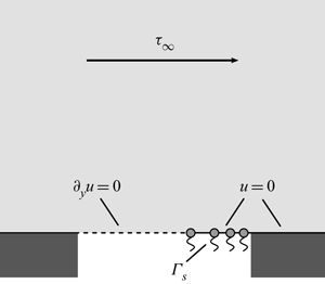
The geometry under investigation is sketched in figure 1(a), with a liquid in Cassie state above a surface composed of an array of solid ridges with periodicity  $2b$ separated by gas-filled cavities of width
  $2a_0$. The gas–liquid interfaces are assumed to remain flat and covered by an insoluble surfactant at mean surface concentration
  $\varGamma _0$. Application of a shear stress in the transverse direction to the cavities induces a flow driving the surfactants towards one side of the cavity, figure 1(b). Since the surfactants are trapped in each cavity and assuming an effectively two-dimensional situation with translational symmetry in a direction normal to the plane of the figure, the total surfactant flux,
  $N_s(x) = u(x,0)\varGamma _s(x) - D_s \partial _x \varGamma _s(x)$, on the gas–liquid interface vanishes at steady state, where
  $u(x,0)$ is the fluid velocity at the interface,
  $\varGamma _s(x)$ the surface concentration of surfactant molecules and
  $D_s$ their surface diffusion coefficient. We shall here focus on the limiting case when convective transport dominates over diffusive transport (large Péclet number,
  $Pe \sim u a / D_s$), such that
 \begin{equation} u(x,0)\varGamma_s(x) = 0, \end{equation}
indicating that either  $\varGamma _s(x)=0$ (uncontaminated interface) or the velocity
  $u(x,0)$ at the interface vanishes (stagnant interface).

Figure 1. (a) Sketch of a unit cell of the geometry with a liquid in Cassie state above a surface composed of a periodic array of solid surface sections (ridges) of width  $2(b-a_0)$ separated by gas-filled cavities (grooves) of width
  $2a_0$. The gas–liquid interface is assumed to be flat and laden with a dilute insoluble surfactant at average surface concentration
  $\varGamma _0$. (b) Application of a shear stress
  $\tau _\infty$ far from the surface drives a Couette flow perpendicular to the grooves, sweeping a section of width
  $2a$ of each gas–liquid interface clean of surfactants, while a section
  $\ell -a$ becomes immobilized by competing shear and Marangoni stress due to surfactant coverage. Then the surface has a pattern of no-stress regions
  ${\mathcal {S}}_0$ of width
  $2a$ alternating with no-slip regions
  $\bar {\mathcal {S}}_0$ of width
  $2(b-a)$. The far-field velocity resembles a plane Couette flow over a surface with effective slip length
  $a\beta$.
This immobilization of the gas–liquid interface results from a balance between viscous shear stress and Marangoni stress due to the spatial variation of the surface tension. For insoluble surfactants (Langmuir monolayers) the surface tension depends on the surfactant coverage via
 \begin{equation} \gamma = \gamma_0-k_B T \varGamma_\infty g(\varGamma_s/\varGamma_\infty), \end{equation}
where  $\gamma _0$ is the surface tension of the uncontaminated surface,
  $k_B$ the Boltzmann constant,
  $T$ the temperature and
  $\varGamma _\infty$ refers to the concentration of a densely packed monolayer;
  $g(\xi )$ is a positive function of the surface coverage
  $\xi =\varGamma _s/\varGamma _\infty$ with
  $g(0)=0$ for which a number of thermodynamic models (equations of state) have been proposed (Lyklema Reference Lyklema2000). For low enough surface concentration,
  $g(\xi )\simeq \xi$ such that
  $\gamma \simeq \gamma _0 -k_B T \varGamma _s$ depends linearly on the surface concentration
  $\varGamma _s$. The tangential stress balance at the gas–liquid interface becomes (Leal Reference Leal2007)
 \begin{equation} \mu \partial_y u|_{y=0} - k_B T\varGamma_\infty \partial_x g(\varGamma_s/\varGamma_\infty) = 0, \end{equation}
where  $\mu$ is the liquid viscosity and we have neglected the influence of the gas trapped in the grooves on the stress balance due to its low viscosity (Schönecker, Baier & Hardt Reference Schönecker, Baier and Hardt2014).
From (2.1) and (2.3) it follows that on the uncontaminated part of the surface the free-slip condition prevails, while the viscous stress is balanced by Marangoni stress on the stagnant contaminated part of the surface. Knowing the velocity field above a surface with alternating segments of no-slip and no-shear boundary conditions allows integration of (2.3) starting from the edge of the surfactant-laden part of the surface, which yields the concentration field  $\varGamma _s(x)$. The width of the stagnant region is then determined by the conservation of surfactant on each groove, such that
 \begin{equation} 2 a_0 \varGamma_0 = \int_a^\ell \varGamma_s(x) \,{\textrm{d}x},\quad\text{with}\ \ell = 2a_0-a. \end{equation}
where  $a$ and
  $\ell$ are unknown but related by
  $2a_0=a+\ell$, since the upper bound
  $\ell$ of the integration coincides with the edge of the groove of width
  $2a_0$, as sketched in figure 1.
Shear-driven incompressible Stokes flow over a planar surface with alternating no-shear and no-slip sections, as required for the present analysis, was investigated by Philip (Reference Philip1972). Before turning to a description of these results and their application in the next sections, a brief look at the critical assumption of convection-dominated surfactant transport is in order.
Langmuir monolayers become fairly rigid for dense surface coverage  $\varGamma _\infty \sim (1 \ldots 10)\ \textrm {nm}^{-2}$ (Lyklema Reference Lyklema2000), corresponding to a size
  $d \sim \varGamma _\infty ^{-1/2} \sim (0.3 \ldots 1)$ nm of the surfactant molecules at the interface. For sufficiently dilute surface coverage,
  $\xi =\varGamma _0/\varGamma _\infty \lesssim 10^{-1}$, values of the surface diffusion coefficient lie in the range
  $D_s \sim (10^{-9} \ldots 10^{-10})\ \textrm {m}^2\ \textrm {s}^{-1}$ (Lyklema Reference Lyklema2000), compatible with a scaling
  $D_s \sim k_B T/(3{\rm \pi} \mu d)$. We are interested in phenomena where viscous stresses are balanced by Marangoni stresses, signified by a Marangoni number
  $Ma \sim k_B T \varGamma _0/(a \tau _\infty )$ of order unity. With a velocity scale
  $u\sim a \tau _\infty /\mu$ on the uncontaminated part of the gas–liquid interface, the product of the Péclet number,
  $Pe \sim u a/D_s$, and Marangoni number thus scales as
  $Pe\,Ma \sim a k_B T\varGamma _0/(\mu D_s) \sim 3{\rm \pi} \xi (a/d)$. Thus, for
  $a \sim 10\ \mathrm {\mu }$m and a surface coverage of
  $\xi \sim 10^{-3}$ we get, as required,
  $Pe\sim 10^2\gg 1$, indicating convection-dominated surfactant transport. At the same time, for aqueous systems with kinematic viscosity
  $\nu \simeq 10^{-6}\ \textrm {m}^2\ \textrm {s}^{-1}$, the Reynolds number
  $Re=(D_s/\nu )Pe$ remains sufficiently small in the range of surface diffusivities given above. Therefore, Stokes flow remains a suitable approximation. Furthermore, with
  $\gamma _0 \sim 10^{-1}\ \textrm {J}\ \textrm {m}^{-2}$ the capillary number
  $Ca=a\tau _\infty /\gamma _0 \sim k_B T \varGamma _0 /( \gamma _0Ma) \sim 10^{-1}\xi /Ma$ remains sufficiently small for the surface deformation to be negligible.
2.1. Shear-driven Stokes flow over a flat surface
With Philip (Reference Philip1972), let us assume two-dimensional Stokes flow over a wall with a single no-shear region of width  $2a$ or with a periodic array of such regions with periodicity
  $2b$, as sketched in figure 1(b). Using the length scale
  $a$ and the velocity scale
  $u_0=a\tau _\infty /\mu$ allows us to introduce dimensionless coordinates
  $(X,Y)=(x/a,y/a)$ and velocities
  $(U,V)=(u/u_0, v/u_0)$ in the upper half-plane,
  $Y>0$. Incompressibility permits us to describe the velocity field
  $(U,V)=(\partial _Y \varPsi , -\partial _X \varPsi )$ in terms of a streamfunction
  $\varPsi (X,Y)$. In the limit of Stokes flow, when inertia can be neglected, the governing equation for the streamfunction becomes the biharmonic equation
  $\varDelta ^2 \varPsi = 0$, where
  $\varDelta =\partial _X^2 + \partial _Y^2$ is the Laplace operator.
Introducing the complex coordinate  $Z=X+\textrm {i}Y$, the no-slip and no-shear boundary regions coincide with the real axis. Philip (Reference Philip1972) showed that shear-driven Stokes flow over a flat surface with alternating sections of no-shear regions,
  ${\mathcal {S}}_0$, and no-slip regions,
  $\bar {{\mathcal {S}}}_0=\mathbb {R}/{\mathcal {S}}_0$, on the real axis is governed by the streamfunction
 \begin{equation} \varPsi(X,Y)=\tfrac{1}{2} Y \,\textrm{Im}[f(Z)],\quad Z=X+\textrm{i}Y, \end{equation}
where  $f$ is an analytic function in the upper half-plane,
  $Y>0$, obeying the boundary conditions
 \begin{align} \textrm{Im}[f(X)] = 0,\ X \in \bar{\mathcal{S}}_0; \quad \textrm{Re}[f'(X)] = 0,\ X \in {\mathcal{S}}_0; \quad \textrm{Re}[f'(Z)] \to 1,\ Y \to \infty. \end{align}
Here,  $f'$ denotes the complex derivative of
  $f$, while
  $\textrm {Re}[\cdot ]$ and
  $\textrm {Im}[\cdot ]$ designate real and imaginary parts, respectively. The Cauchy–Riemann conditions,
  $\textrm {Re}[f']=\partial _X \,\textrm {Re}[f]= \partial _Y \,\textrm {Im}[f]$ and
  $\textrm {Im}[f'] = \partial _X \,\textrm {Im}[f]=-\partial _Y \,\textrm {Re}[f]$, allow us to rewrite the boundary conditions (2.6a–c) as conditions for
  $\textrm {Im}[f]$ and its derivatives only. They furthermore establish that both the real and imaginary parts of an analytic function are harmonic functions,
  $\varDelta \textrm {Im}[f] = \varDelta \textrm {Re}[f]= 0$, such that (2.6a–c) can also be viewed as boundary conditions for the Laplace equation for
  $\textrm {Im}[f]$.
A direct calculation shows that  $\varDelta \varPsi = \textrm {Re}[f']$. Since the right-hand side is a harmonic function, the streamfunction (2.5) indeed solves the biharmonic equation
  $\varDelta ^2\varPsi =0$ for incompressible Stokes flow. The corresponding velocity field
 \begin{equation} (U,V)=(\partial_Y \varPsi, -\partial_X \varPsi)=\tfrac{1}{2}(\textrm{Im}[f]+Y\,\textrm{Re}[f'],-Y\,\textrm{Im}[f']) \end{equation}
thus solves the incompressible Stokes equation with the inherited boundary conditions
 \begin{equation} \left.\begin{gathered} V(X,0) = 0,\quad \text{for}\ X \in \mathbb{R} \\ U(X,0) = 0,\quad \text{for}\ X \in \bar{\mathcal{S}}_0 \\ \partial_Y U|_{Y=0} = 0,\quad \text{for}\ X \in {\mathcal{S}}_0 \\ \partial_Y U \to 1,\quad \text{for}\ Y \to \infty \end{gathered}\right\} \end{equation}
on the real axis and in the far field. Specifying a suitable analytic function  $f$ obeying (2.6a–c) thus determines the flow over the surface. In order to ensure a pure Couette flow far from the surface,
  $\textrm {Im}[f']$ must vanish sufficiently fast such that
 \begin{equation} V \to 0, \quad \text{for}\ Y \to \infty. \end{equation}
 For a single groove of width  $2a$,
$2a$,  ${\mathcal {S}}_0 = \{X\in \mathbb {R}\,|\, X^2<1\}$, Philip (Reference Philip1972) showed that
 \begin{equation} f_{s}(Z) = \sqrt{Z^2-1} \end{equation}
is the appropriate analytic function obeying the boundary conditions (2.6a–c) and (2.9).
For an evenly spaced array of grooves of width  $2a$ and periodicity
  $2b=2aB$,
  ${\mathcal {S}}_0 = \{X\in \mathbb {R}\,|\,(X+2nB)^2<1,\ \text {for all}\ n\in \mathbb {Z}\}$, the corresponding function is (Philip Reference Philip1972)
 \begin{equation} f_{a}(Z)=\frac{1}{\alpha}\arccos\left(\frac{\cos(\alpha Z)}{\cos(\alpha)}\right),\quad \alpha=\frac{\rm \pi}{2}\frac{a}{b}. \end{equation}
In the limit of large spacing between the grooves,  $b \gg a$,
 \begin{equation} \lim_{\alpha\to 0^+}f_a(Z) = f_{s}(Z), \end{equation}
indicating that at sufficient spacing the flow in the vicinity of each groove in the array resembles the flow over a single groove.
Streamlines for the flow over a single groove and an array of grooves with  $a/b=0.5$ and 0.9 are shown in figure 2. As can be seen, for both (2.10) and (2.11) the flow becomes parallel to the wall at distances of a few times the feature size of structures on the wall. The flow thus resembles a pure Couette flow with a constant shear stress far away from the wall, which becomes modified by the presence of the grooves in a relatively narrow zone close to the wall. For arrays of grooves, this modification results in a scaling of the tangential velocity
  $U\simeq Y+\beta$ far from the wall, with an effective slip length
  $\beta =- (2\alpha )^{-1} \ln (\cos (\alpha ))$ (Philip Reference Philip1972).


We note in passing that despite the divergence of the pressure  $p-p_0=-\tau _\infty \textrm {Im}[f']$ (where
  $p_0$ is a constant reference pressure) in the vicinity of points of transition between the no-slip and no-shear interfaces, the normal stress
  $p-2\mu \partial _y v=p_0+\tau _\infty Y\,\textrm {Re}[f'']$ reduces to the constant
  $p_0$ on the interface (Michael Reference Michael1958; Richardson Reference Richardson1970; Harper Reference Harper1992), as further discussed in appendix A.
3. Results and discussion
From the previous section it is now straightforward to obtain the surface concentration  $\varGamma _s$ from the stress balance (2.3) and to evaluate its conservation (2.4) to obtain a relation between the applied stress
  $\tau _\infty$ and the fraction
  $(a/a_0)$ of uncontaminated gas–liquid interface on each groove.
With the streamfunction (2.5) the shear stress at the wall at  $Y=0$ becomes
 \begin{equation} \left.\mu \partial_y u \right|_{y=0} = \tau_\infty \partial_Y^2 \varPsi(X,0) = \tau_\infty \left.\partial_Y \,\textrm{Im}[f(Z)]\right|_{Z=x/a} = \tau_\infty \left.\partial_X \,\textrm{Re}[f(Z)]\right|_{Z=x/a}, \end{equation}
where again the Cauchy–Riemann conditions were used. Integrating the stress balance (2.3), starting at  $x=a$ with
  $\varGamma _s(a)=0$ yields
 \begin{equation} g(\varGamma_s(x)/\varGamma_\infty)=\frac{a \tau_\infty}{k_B T \varGamma_\infty} \left.f(X)\right|_{X=x/a} \quad \text{on}\ \bar{\mathcal{S}}_0, \end{equation}
where we have used (2.6a–c) to see that  $f(X)$ is a real function on the no-slip sections
  $\bar {\mathcal {S}}_0$. Equation (3.2) determines the surfactant concentration profile
  $\varGamma _s(x)$ at the gas–liquid interface.
Defining the Marangoni number as a characteristic ratio between Marangoni stress and shear stress with  $a_0$ as the length scale,
 \begin{equation} Ma = \frac{k_B T\varGamma_0}{a_0\tau_\infty}, \end{equation}
the conservation of surfactant on each groove, (2.4), yields the relation
 \begin{equation} Ma = \frac{1}{2}\left(\frac{a}{a_0}\right)^2 \int_1^{(2({a_0}/{a})-1)} g^{-1}[f(X)]\,\textrm{d} X. \end{equation}
between  $Ma$ and
  $(a/a_0)$, where we have tacitly assumed that the inverse
  $g^{-1}$ exists.
From now on, we will focus on the simplest thermodynamic model of an ideal Langmuir monolayer generally applicable at sufficiently low surface concentrations, i.e. we assume the surface tension to depend linearly on the surfactant load with  $g(\xi )=\xi =\varGamma _s/\varGamma _\infty$ (Lyklema Reference Lyklema2000). However, we emphasize that this is not a fundamental limitation of the presented method which can be adapted to more general equations of state for the surfactant molecules.
3.1. Single groove
For the single groove with  $f_{s}(Z)$ from (2.10), the integral in (3.4) is easily evaluated and we obtain the relation
 \begin{equation} Ma = Ma_{s}\left[\frac{a}{a_0}\right] := \frac{1}{4}\left(\frac{a}{a_0}\right)^2 \left[X\sqrt{X^2-1}-\text{arcosh}\left(X\right)\right]_{X=2({a_0}/{a})-1}, \end{equation}
shown as a solid line in figure 3(a). For a given Marangoni number this relation thus allows us to establish the width  $2a$ of the section of the groove that is cleared of surfactants due to the flow. The corresponding velocity field is then given by (2.7) together with (2.10). For
  $Ma \geq 1$ (small
  $\tau _\infty$) the interface remains fully covered by surfactant, and the flow becomes a pure Couette flow over a no-slip surface, where Marangoni stresses balance the shear stress
  $\tau _\infty$ everywhere on the gas–liquid interface. For small
  $Ma$ (large
  $\tau _\infty$) almost the entire interface gets swept clean of surfactant. However, in this limit care must be exercised, since surfactant concentrations may become large, while (3.5) is only valid in the dilute limit where the linear equation of state applies.

Figure 3. (a) Relation between  $Ma=k_B T\varGamma _0/(a_0\tau _\infty )$ and
  $a/a_0$ according to (3.5) for a single groove (solid line) and according to (3.6) for an array of grooves with gas–liquid interface fractions
  $a_0/b=\{0,0.6,0.8,0.9,0.96,1\}$. (b) Dimensionless effective slip length
  $\beta$ according to (3.9a,b) as a function of
  $Ma$, (3.6), for flow over a periodic array of grooves with
  $a_0/b=\{0.6,0.8,0.9,0.96,1\}$.
3.2. Array of grooves
For a periodic array of grooves of width  $2a$ and period
  $2b$ we obtain the relation
 \begin{align} Ma = Ma_{a}\left[\frac{a}{a_0},\frac{a_0}{b}\right] := \frac{1}{2}\left(\frac{a}{a_0}\right)^2 \int_1^{(2({a_0}/{a})-1)} \frac{1}{\alpha}\arccos\left( \frac{\cos(\alpha X)}{\cos(\alpha)} \right) \textrm{d} X,\quad \alpha=\frac{\rm \pi}{2}\frac{a}{a_0}\frac{a_0}{b}. \end{align}
Apart from the ratio  $(a/a_0)$ between uncontaminated and total interface area, in this case the right-hand side also depends on the ratio
  $(a_0/b)$ of the area occupied by grooves and the total wall area.
Two limiting cases allow us to evaluate the right-hand side of (3.6). As already noted after (2.12), for  $b \gg a_0 \geq a$ each groove can be treated independently such that the flow field and hence (3.6) reverts to the result for a single groove (3.5),
 \begin{equation} \lim_{(a_0/b) \to 0^+} Ma_{a} \left[\frac{a}{a_0},\frac{a_0}{b}\right] = Ma_{s}\left[\frac{a}{a_0}\right]. \end{equation}
On the other hand, when the original surface has a large free surface fraction,  $a_0/b\approx 1$, the no-slip surface
  $\bar {\mathcal {S}}_0$ consists almost entirely of immobilized surfactants such that the integral in (3.4) extends over the whole width to
  $\ell /a = 2a_0/a-1 \approx 2b/a-1$. In other words, the width of the solid surface sections is negligible. In this limit the integral is easily evaluated by inspecting the symmetry of the integrand, resulting in
 \begin{equation} \lim_{(a_0/b)\to 1^-} Ma_{a} \left[\frac{a}{a_0},\frac{a_0}{b}\right] = 1-\frac{a}{a_0}. \end{equation}
 The relation (3.6) between  $Ma$ and
  $a/a_0$ can be evaluated numerically and is shown in figure 3(a) for several values of
  $a_0/b$, including the two limiting cases discussed. As can be observed, for a given value of
  $Ma$, all values of
  $a/a_0$ fall within a narrow band for all values of
  $a_0/b$. The corresponding flow field across an interface that is partially covered with surfactants then again follows from (2.7) with (2.11). As for a single groove, for
  $Ma \ge 1$ the gas–liquid interfaces remain entirely covered by surfactant, with Marangoni stress balancing the shear stress, such that the flow becomes a Couette flow over a no-slip surface with
  $\beta =0$.
As mentioned, far from the microstructured surface the velocity field has the form of a Couette flow over a surface with effective slip,
 \begin{equation} \frac{y}{a}\gg 1: \quad u \simeq \frac{\tau_\infty}{\mu} \left(y+a\beta\right),\quad \beta = - \frac{1}{2\alpha} \ln\left(\cos\left(\alpha\right)\right),\quad \alpha=\frac{\rm \pi}{2}\frac{a}{b}, \end{equation}
where  $\beta$ is the non-dimensional effective slip length (Philip Reference Philip1972). This relation between far-field velocity and shear stress is accessible experimentally in a suitable viscosimeter set-up, as long as the plane of applied shear remains outside of the narrow zone in the vicinity of the wall where the velocity field is modified appreciably due to the presence of the grooves. For several values of
  $a_0/b$, the effective slip length
  $\beta$ is shown in figure 3(b) as a function of
  $Ma$ according to (3.6). For
  $a_0/b = 1$ the effective slip length diverges when
  $Ma \to 0$. For surfaces with a large free surface fraction
  $a_0/b$ the effective slip length can thus become strongly dependent on the applied shear stress
  $\tau _\infty$ even at small surfactant concentrations
  $\varGamma _0$. Likewise, considering a fixed applied shear stress, such surfaces are very sensitive to small amounts of contaminants. Both facts are reflected in the large absolute values of
  $\textrm {d} \beta / \textrm {d} Ma$ when
  $Ma \rightarrow 0$.
Throughout this work, a Langmuir monolayer is assumed. When using a linear equation of state, (3.2) always has a solution  $\varGamma _s(x)$, no matter how large the shear stress exerted on the gas–liquid interface is. In other words, the Marangoni stress in the monolayer can always balance the shear stress. This is of course an artifact of the linearization. In realistic Langmuir monolayers a specific type of transformation or collapse occurs when the stress exceeds a critical value (Lee Reference Lee2008). Either the surfactant-covered surface starts to buckle, or the monolayer collapses and forms multilayer domains. The buckling scenario can be modelled by regarding the monolayer as an elastic sheet (Lee Reference Lee2008), which, however, has its limitations when more complex morphology transitions such as the formation of multilayer domains become relevant. Using realistic equations of state, the onset of such processes should become apparent by a critical shear stress above which (3.2) no longer has a solution.
We note that a no-slip boundary condition was assumed on both the solid sections and the parts of the gas–liquid interface rendered immobile due to presence of surfactants. Since the intrinsic slip length for flow of a liquid over solid surfaces and over surfactant-covered surfaces is reported to lie in the nanometre range or below (Cottin-Bizonne et al. Reference Cottin-Bizonne, Barentin, Charlaix, Bocquet and Barrat2004; Joly, Detcheverry & Biance Reference Joly, Detcheverry and Biance2014) this does not affect the results presented in this paper as long as the feature size on the wall is in the micrometre range.
It should also be noted that the far-field velocity (3.9a,b) relies on a periodic array of grooves of the same width. For corresponding experiments it is thus important to ensure that the surface coverage  $\varGamma _0$ is identical on each groove, as this affects the width of the individual sections swept clean of surfactants.
4. Conclusions and outlook
The influence of insoluble surfactants on the shear-driven flow over a microstructured surface with transverse grooves in Cassie state was quantified in the regime of large Péclet numbers based on an analytical model. This influence pertains both to the local flow and surfactant distribution at the gas–liquid interface as well as the effective slip velocity observable far from the surface. Among others, the results will help quantifying the deteriorating effects of surface-active species when utilizing superhydrophobic surfaces for drag reduction.
In the case of a periodic array of grooves, the far-field velocity (3.9a,b) already becomes an excellent approximation for the velocity at distances of only a few times the structure periodicity  $2b$ away from the wall. Consequently, the results presented above are also applicable to pressure-driven Poiseuille flow between parallel plates as long as the plate separation is a few times the periodicity of the underlying surface. The same is true for Couette flow at sufficiently large distances between two surfaces. In both cases, one obtains the flow enhancement (or corresponding drag reduction) compared to flow in a channel bounded by flat solid walls by replacing the no-slip boundary condition on the wall by a Navier-slip boundary condition that contains the effective slip length corresponding to the Marangoni number derived from the applied far-field shear stress.
It has been suggested that superhydrophobic surfaces can be employed as a means for pumping liquid in conjunction with thermocapillary flow due to a temperature gradient along the gas–liquid interface (Baier, Steffes & Hardt Reference Baier, Steffes and Hardt2010), diffusioosmotic flow (Huang et al. Reference Huang, Cottin-Bizonne, Ybert and Bocquet2008) or electroosmotic flow (Squires Reference Squires2008; Belyaev & Vinogradova Reference Belyaev and Vinogradova2011; Steffes, Baier & Hardt Reference Steffes, Baier and Hardt2011; Schönecker & Hardt Reference Schönecker and Hardt2014). It should be interesting to extend the results of the present paper to such situations in order to study the impact of surfactants in these cases.
For a thorough discussion of the influence of soluble surfactants (Gibbs monolayers) under a wide range of flow configurations we refer to the article by Landel et al. (Reference Landel, Peaudecerf, Temprano-Coleto, Gibou, Goldstein and Luzzatto-Fegiz2020), which our model complements by an analytically solvable case.
Acknowledgements
We are indebted to S. Dehe and M. Eigenbrod for stimulating discussions.
Declaration of interests
The authors report no conflict of interest.
Appendix A. Surface stress at the gas–liquid interface
In this appendix we briefly study the stress singularities at the gas–liquid interface and the impact on surface deformation for the flows considered in this work. For a flow given by the streamfunction (2.5), the components of the viscous stress tensor (Bird, Stewart & Lightfoot Reference Bird, Stewart and Lightfoot2007),  $\tau _{ij}=-\mu (\partial _i u_j + \partial _j u_i)$, are
 \begin{equation} \tau_{xx} = -\tau_{yy} = -\tau_\infty ( \textrm{Im}[f'] + Y \,\textrm{Re}[f''] ), \end{equation}
 \begin{equation}\tau_{xy} =\tau_{yx}=\tau_\infty (-\textrm{Re} [f'] + Y \,\textrm{Im} [f'']). \end{equation}
The corresponding pressure field is obtained by integrating the Stokes equation,  $\partial _i p = -\partial _j\tau _{ji}$, as
 \begin{equation} p=p_0 - \tau_\infty \textrm{Im}[f'], \end{equation}
where  $p_0$ is a constant reference pressure.
For Couette flow over a single slot described by (2.10),  $f_s'(Z)=Z/\sqrt {Z^2-1}$ and
  $f_s''(Z)=-(Z^2-1)^{-3/2}$, such that in the vicinity of the point of transition between the no-shear and no-slip regions at the gas–liquid interface,
  $Z=1+R \,\textrm {e}^{\textrm {i}\varphi }$, both the pressure and the components of the viscous stress tensor exhibit a square-root singularity,
  $|p|\sim 1/\sqrt {R}$ and
  $|\tau _{ij}|\sim 1/\sqrt {R}$. Nevertheless, the total normal stress
 \begin{equation} {\rm pi}_{yy} = p+\tau_{yy} = p_0+\tau_\infty Y\,\textrm{Re}[f''] \end{equation}
reduces to the constant  $p_0$ on the interface at
  $Y=0$, not only away from these singular points where
  $\textrm {Re}[f'']$ remains finite, but even in the vicinity of these points (Michael Reference Michael1958; Richardson Reference Richardson1970; Harper Reference Harper1992). In particular, at
  $Z=1+R \,\textrm {e}^{\textrm {i}\varphi }$ the normal stress has the form
  $({\rm \pi} _{yy}-p_0)/\tau _\infty \approx -\sin (\varphi )\{\cos (3\varphi /2)/\sqrt {8 R} + O(\sqrt {R})\}$, which vanishes on the interface at
  $\varphi =0,{\rm \pi}$ for any
  $R>0$. However, the limit
  $\lim _{Z\to 1} {\rm \pi}_{yy}$ remains undefined as it depends on the path taken, with a square-root divergence when approaching this point from the bulk of the liquid, while vanishing on approach along the gas–liquid interface itself.
In order to ensure that the point  $Z=1$ does not give a finite contribution to the force on the interface, we calculate the
  $y$-component of the momentum flux through a small semi-circular arc,
  $\gamma =\{aZ \,|\, Z=1+R\,\textrm {e}^{\textrm {i}\varphi },\ 0\le \varphi \le {\rm \pi}\}$, of radius
  $r=aR$ around this point,
 \begin{equation} f_y(R) = \boldsymbol{e}_y \boldsymbol{\cdot} \int_0^{\rm \pi} \left( \rho \boldsymbol{u}\boldsymbol{u}+\boldsymbol{\rm \pi} \right) \boldsymbol{\cdot}\boldsymbol{n}(\varphi)aR \,\textrm{d}\varphi, \end{equation}
where  $\boldsymbol {e}_i$ are unit vectors in the
  $i$-direction,
  $\boldsymbol {n}(\varphi )=\cos (\varphi )\boldsymbol {e}_x+\sin (\varphi )\boldsymbol {e}_y$ is the unit normal on the semi-circular arc,
  $\boldsymbol {u}=u_i\boldsymbol {e}_i$ is the velocity and
  $\boldsymbol {{\rm \pi} }$ is the total stress tensor with components
  ${\rm \pi} _{ij}=p \delta _{ij}+\tau _{ij}$. Since at
  $Z=1+R \,\textrm {e}^{\textrm {i}\varphi }$,
  $|\boldsymbol {u}|\sim \sqrt {R}$, while
  $|\boldsymbol {{\rm \pi} }|\sim 1/\sqrt {R}$ to lowest order in
  $R$,
$R$,  $|\,f_y(R)| \sim \sqrt {R}$ vanishes in the limit
  $R\to 0$, establishing that the singular point does not contribute to the deformation of the interface. Assuming the pressure in the gas phase below the gas–liquid interface to agree with the reference pressure
  $p_0$, the interface thus remains flat.
The same holds for Couette flow over an evenly spaced array of grooves according to (2.11). Indeed, the streamfunction (2.5) at  $Z=1+R \,\textrm {e}^{\textrm {i}\varphi }$ has the form
  $\varPsi \sim R^{3/2} \sin (\varphi /2) \sin (\varphi )$ for small
  $R$ for both a single groove and an array of grooves.
The assumption of a flat interface for shear flow over the surfaces considered in this work is thus self-consistent. Nevertheless, since the perfectly flat interface remains an idealization and the pure Couette flow considered here may be an approximation to some other far-field boundary condition, we note that our parameter estimate right before § 2.1 indicates that the capillary number remains small within the parameter region of interest for this work, such that deformations of the interface remain sufficiently small.


