


1. Introduction
Our study is motivated by the understanding of large scale nearly axisymmetric vortices in the atmosphere, such as tropical cyclones, also referred to as hurricanes or typhoons. Oscillations have been observed near the eye of actual tropical cyclones (e.g. Harlow & Stein Reference Harlow and Stein1974; Chen et al. Reference Chen, Lu, Li and Wen2015). These are reminiscent of inertial waves and exhibit similar periods (Atkinson, Davidson & Perry Reference Atkinson, Davidson and Perry2019). A clean cut mathematical model is needed in order to investigate these waves. We therefore investigate inertial wave activity in a penny shaped cylinder in solid body rotation for which the angular velocity of the container is abruptly changed.
In Oruba, Soward & Dormy (Reference Oruba, Soward and Dormy2020), we investigated the inertial wave response during spin-down in a shallow cylinder height  $H$, of large radius
  $L\,(\gg H)$, equivalently
 \begin{equation} \ell\equiv L/H \gg 1, \end{equation}
by consideration of a ‘reduced model’. Here, we consider the complete problem. On the one hand, we refrain from repeating some of the references cited in Oruba et al. (Reference Oruba, Soward and Dormy2020), which apply equally here. On the other, as we need to refer extensively to equations (say ( $x.y$)), sections (say §
 $x$) and figures (say figure
  $x$) from Oruba et al. (Reference Oruba, Soward and Dormy2020) (say
  ${O}$), we use the notation ‘(
 ${O}$:
  $x.y$)’, ‘§
 ${O}$:
 $x$’ and ‘figure
  ${O}$:
 $x$’ respectively to identify them.
Our cylindrical container is filled with constant density fluid of viscosity  $\nu$ and rotates rigidly with angular velocity
  $\varOmega$ about its axis of symmetry, the frame, relative to which our analysis is undertaken; the Ekman number is small
 \begin{equation} E=\nu/(H^2\varOmega)\ll 1. \end{equation}
Initially, at time  $t^{\dagger} =0$, the fluid itself rotates rigidly at the slightly larger angular velocity
  ${\textit {Ro}}\,\varOmega$, in which the Rossby number
  ${\textit {Ro}}$ is sufficiently small (
 ${\textit {Ro}}\ll E^{1/4}$) for linear theory to apply. Relative to cylindrical polar coordinates,
  $(r^{\dagger} ,\theta ^{\dagger} ,z^{\dagger} )$, the top boundary (
 $r^{\dagger} < L$,
  $z^{\dagger} =H$) and the sidewall (
 $r^{\dagger} =L, 0 < z^{\dagger} < H$) are impermeable and stress free. The bottom boundary (
 $r^{\dagger} < L, z^{\dagger} =0$) is rigid. For that reason alone the initial state of relative rigid rotation
  ${\textit {Ro}}\,\varOmega$ of the fluid cannot persist and the fluid spins down to the final state of no rotation relative to the container, as
  $t^{\dagger} \to \infty$. We describe the transient relative motion, velocity
  ${\boldsymbol{v}} ^{\dagger}$, by its cylindrical components oriented by the rotation axis, which we partition into its horizontal
  ${\boldsymbol{v}} ^{\dagger} _{\perp }=[u^{\dagger} ,v^{\dagger} ]$ and vertical
  $w^{\dagger}$ components.
Whereas an actual tropical cyclone is in essence living in an unbounded flow (at the surface of a sphere), models of axisymmetric geophysical vortices in general (e.g. Williams Reference Williams1968; Rotunno Reference Rotunno1979; Read Reference Read1986a,Reference Readb; Rotunno Reference Rotunno2014) and of tropical cyclones in particular (e.g. Rotunno & Emanuel Reference Rotunno and Emanuel1987; Montgomery, Snell & Yang Reference Montgomery, Snell and Yang2001) are in essence bounded. The same would be true of any experimental set-up. In the particular set-up investigated here, inertial wave activity is triggered by the outer bounding wall. In a true cyclone, they will be triggered by other disturbances (such as non-axisymmetric heterogeneities) but will be equally important. In practice, they may also interact nonlinearly (e.g. Yarom & Sharon Reference Yarom and Sharon2014). Here, we restrict our attention to the exact linear ( ${\textit {Ro}}\ll 1$) solution for a bounded flow, relevant to either a numerical model or laboratory experiment, both bounded. We describe mathematically how the waves triggered at the outer boundary propagate toward the axis and reasonably expect that some of the qualitative wave behaviour predicted will not simply depend on our chosen forcing but apply equally to real tropical cyclones. Indeed, we believe that our waves can shed light on understanding the inertial wave activity observed near the axis of cyclones (e.g. Chen et al. Reference Chen, Lu, Li and Wen2015).
Inertial waves in confined flows, driven by the relative motion of boundaries, is of continued topical interest, from both experimental and theoretical points of view (see Klein et al. (Reference Klein, Seelig, Kurgansky, Ghasemi V., Borcia, Will, Schaller, Egbers and Harlander2014), Kurgansky et al. (Reference Kurgansky, Seelig, Klein, Will and Harlander2020) and references therein). The special case of linear spin-down, manifest primarily by a quasi-geostrophic (QG) flow (largely time-dependent rigid rotation) caused by axial vortex line shortening due to blowing from the Ekman layers, is well understood (see e.g. Benton & Clark Reference Benton and Clark1974; Duck & Foster Reference Duck and Foster2001). However, the secondary generation of inertial waves during spin-down has received less attention. Though, in the case of a cylinder, their wave spectrum and viscous decay rates are well understood (see e.g. Kerswell & Barenghi (Reference Kerswell and Barenghi1995), Zhang & Liao (Reference Zhang and Liao2008) and references therein) we are only aware of one study (Cederlöf Reference Cederlöf1988) that addresses the issue of wave amplitude analytically.
Our development builds on a laterally unbounded model ( $L\to \infty$) studied in considerable detail by Greenspan & Howard (Reference Greenspan and Howard1963), for which a useful summary and clarifying description are given in §§ 2.3 and 2.4 of Greenspan (Reference Greenspan1968). We emphasise, at the outset, that mathematically our use of a stress-free boundary at
  $z^{\dagger} =H$ is equivalent to theirs on doubling our gap height and applying no-slip boundary conditions at
  $z^{\dagger} =2H$ instead. The equivalence follows from symmetries,
  $z^{\dagger} \mapsto 2H-z^{\dagger}$, about the mid-plane
  $z^{\dagger} =H$. Greenspan & Howard (Reference Greenspan and Howard1963) also considered the role of the outer rigid boundary at
  $r^{\dagger} =L$ and particularly the boundary layer structure there.
The spin-down process operates on three time scales identified by
 \begin{equation} \varOmega t^{\dagger}=\left\{\begin{array}{@{}ll} O(1), & \mbox{rotation or inertial wave time,}\\ O(E^{{-}1/2}), & \mbox{spin-down time,}\\ O(E^{{-}1}), & \mbox{transverse diffusion time.} \end{array}\right. \end{equation}
We will refer to these regimes repeatedly.
Oruba, Soward & Dormy (Reference Oruba, Soward and Dormy2017) pointed out that a QG-layer, close to the outer  $r^{\dagger} =L$ boundary, spreads inwards towards the
  $r^{\dagger} =0$ axis broadening indefinitely. Curiously, when that outer boundary is stress free, the returning meridional flow is not impeded by boundary friction. So, to a small extent, rather than promoting spin-down by compressing axial vortex lines, the opposite tends to happen. The consequence of this weak tendency is to slightly slow spin-down on the long transverse diffusion time scale
  $\varOmega t^{\dagger} =O(E^{-1})$. Here, and in our previous work (Oruba et al. Reference Oruba, Soward and Dormy2020), we are not concerned with that QG-development, but rather focus attention on the evolution of inertial waves triggered simply by the impermeable boundary condition
  $u^{\dagger} =0$ at
  $r^{\dagger} =L$ on the shorter time scales
  $\varOmega t^{\dagger} \ll E^{-1}$. For that, whether the lateral boundary
  $r^{\dagger} =L$ is no slip or stress free is irrelevant and has no influence on the inertial wave activity ‘triggered’ by the blocking of the radial flow found in the unbounded domain
  $L\to \infty$. Fortunately, to compare our inertial wave predictions with the results of direct numerical simulation (DNS) based on the entire governing equations, we are able to filter out the mainstream QG-contribution (as well as the inertial wave contribution, with frequency close to 2, in the trigger flow identified by Greenspan Reference Greenspan1968) to expose only the triggered inertial waves. The filtered waves are the same whether the outer boundary
  $r^{\dagger} =L$ is no slip or stress free.
In short, our approach builds on the idea that the radial outflow for the unbounded case is simply blocked,  $u^{\dagger} =0$ at
  $r^{\dagger} =L$ with, at leading order, the stress boundary condition only affecting the QG-flow contribution studied by Oruba et al. (Reference Oruba, Soward and Dormy2017). Our asymptotic analysis only applies when
  $\varOmega t^{\dagger} \ll E^{-1}$. Oruba et al. (Reference Oruba, Soward and Dormy2020) ignored the early time
  $\varOmega t^{\dagger} =O(1)$ behaviour. Although this is adequate to capture the main features of the triggered wave solution, it is not asymptotically correct. For surprisingly the
  $\varOmega t^{\dagger} =O(1)$ behaviour of the unbounded flow has a persistent influence on the solution. Its most evident consequences are a phase lag and smaller amplitude of the Oruba et al. (Reference Oruba, Soward and Dormy2020) triggered waves relative to the asymptotically correct wave solution derived here.
In order to make our notation relatively compact at an early stage, we use  $H$ and
  $\varOmega ^{-1}$ as our unit of length and time respectively, and introduce
 \begin{equation} r^{\dagger}=Hr,\quad z^{\dagger}=Hz,\quad \varOmega t^{\dagger}=t,\quad {\boldsymbol{v}}^{\dagger}={\textit{Ro}}\,L\varOmega {\boldsymbol{v}}, \end{equation}
in which, for our unit of relative velocity  ${\boldsymbol{v}} ^{\dagger}$, we have adopted the velocity increment
  ${\textit {Ro}}\,L \varOmega$ of the initial flow at the outer boundary
  $r^{\dagger} =L$. The cylindrical component axisymmetric velocity decomposition becomes
 \begin{equation} {\boldsymbol{v}}(r,z,t)=[{\boldsymbol{v}}_{{\perp}},w]\quad \mbox{with}\ {\boldsymbol{v}}_{{\perp}}=[u,v] \end{equation}
and, on introduction of the meridional flow streamfunction  $r\chi$, we have
 \begin{equation} u={-}\displaystyle\frac{\partial{\chi}}{\partial{z}},\quad w=\displaystyle\frac{1}{r}\displaystyle\frac{\partial{(r\chi)}}{\partial{r}}. \end{equation}
 In this Introduction, we summarise and expand on the results of Greenspan & Howard (Reference Greenspan and Howard1963), as needed to properly understand the nature of the unbounded,  $\ell =L/H\to \infty$, spin-down flow which provides the inertial wave trigger in the bounded case at
  $r=\ell$. Like Greenspan & Howard (Reference Greenspan and Howard1963), our development relies heavily on the Laplace transform (LT), an operation
  ${\mathcal {L}}$ leading to values denoted by the
  $\hat {\,}$ accent, e.g.
 \begin{equation} {\hat {\boldsymbol{v}}}(r,z,p)={\mathcal{L}}\{{\boldsymbol{v}}\}\equiv \int_0^\infty {\boldsymbol{v}}(r,z,t)\exp({-}pt)\,{\mathrm d} t \end{equation}
with inverse-LT
 \begin{equation} {\boldsymbol{v}}(r,z,t)={\mathcal{L}}^{{-}1}\{{\hat {\boldsymbol{v}}}\} \equiv \displaystyle\frac{1}{2{\rm \pi} {\mathrm i}}\int_{-{\mathrm i}\infty}^{{\mathrm i}\infty}{\hat {\boldsymbol{v}}}(r,z,p)\exp(pt)\,{\mathrm d} p. \end{equation}
The complete LT-solution of the  $\ell \to \infty$ problem is given by (3.4), (3.5) of Greenspan & Howard (Reference Greenspan and Howard1963). Crucially, the LTs involve cut points at
  $p=\pm 2{\mathrm i}$, exemplified by the factors
  $(p \mp 2 {\mathrm i})^{1/2}$ which appear in their equations (3.6). The cut points are illusory and not part of the solution, which only possesses poles. In the small Ekman number limit
  $E\ll 1$, a pole near
  $p=0$ identifies the QG-spin-down mode, while an infinite sequence of densely packed poles to the left of the ‘illusory’ cuts at
  $p=\pm 2{\mathrm i}$ identifies modes with distinct viscous decay rates with frequencies close to
  $2$ (see Greenspan & Howard Reference Greenspan and Howard1963, (3.7), (3.8)). The latter pole family is needed to properly resolve late time behaviour,
  $t=O(E^{-1})$. At shorter times
  $t < O(E^{-1})$ a different tactic for the LT-inversion (see Greenspan & Howard Reference Greenspan and Howard1963, p. 389, 390) which essentially reinstates the ‘illusory’ cuts, is more useful. That strategy can only be undertaken with considerable caution, as the asymptotic approach has limitations that must be clearly understood. To that end, we build the picture slowly through the survey §§ 1.1, 1.2 (essentially a considerable expansion of Greenspan (Reference Greenspan1968), §§ 2.3 and 2.4, respectively, with an alternative perspective) of a hierarchy of problems that highlight the main ideas. Then, in § 1.3, we identify (1.30) as an approximation to the inertial wave trigger, sufficiently accurate for our purposes over the entire time
  $0 < t\ll E^{-1}$. We outline the organisation of our paper in § 1.4.
1.1. The transient Ekman layer
The transient Ekman layer, in the half-space  $z>0$ above a rigid boundary
  $z=0$, is well known (see e.g. Greenspan Reference Greenspan1968, § 2.3). Still, we provide here a summary in order to develop our notation and highlight features upon which we will build. Significantly, as the LT-solution ((1.12) below) involves both a pole at
  $p=0$ and cuts at
  $p=\pm 2{\mathrm i}$, we may immediately identify the seeds of spin-down and inertial wave generation between parallel planes. For that, the cuts are strictly removed by the inclusion of an upper boundary, as previously mentioned.
We consider the axisymmetric flow in the self-similar form
 \begin{equation} {\boldsymbol{v}}_\perp=(r/\ell)[{\mathfrak{u}}(z,t),{\mathfrak{v}}(z,t)], \quad w=(1/\ell)\,{\mathfrak{w}}(z,t), \end{equation}
that solves
 \begin{equation} \partial_t{\mathfrak{u}}-2({\mathfrak{v}}-1)=E\partial^2_z{\mathfrak{u}}, \quad \partial_t{\mathfrak{v}}+2\,{\mathfrak{u}}=E\partial^2_z{\mathfrak{v}} \end{equation}
subject to  $[{\mathfrak {u}},{\mathfrak {v}}] =[0,1]$ at
  $t=0$, while subsequently
  $[{\mathfrak {u}},{\mathfrak {v}}] =[0,0]$ at
  $z=0$ and
  $[{\mathfrak {u}},{\mathfrak {v}}] \to [0,1]$ as
  $z\uparrow \infty$ for
  $t>0$. Of interest to us is the horizontal boundary layer volume flux deficit
 \begin{equation} -E^{1/2}\displaystyle\frac{r}{\ell}\left[{\mathfrak{U}}(t),{\mathfrak{V}}(t)\right]=\displaystyle\frac{r}{\ell}\int_0^\infty[{\mathfrak{u}},{\mathfrak{v}}-1]\,{\mathrm d} z. \end{equation}
By mass continuity, the outflow velocity  $E^{1/2}{\mathfrak {W}}/\ell$ from it is determined from
 \begin{equation} {\mathfrak{W}}(t)\equiv E^{{-}1/2}{\mathfrak{w}}_{z\uparrow\infty}=2{\mathfrak{U}}(t). \end{equation}
The minus sign in (1.9) is motivated by our application to spin-down between two unbounded parallel plates,  $0 < z < 1$, in the next § 1.2.
In terms of the complex combinations
 \begin{equation} {\mathfrak{z}}^\pm(z,t)={{\mathfrak{u}}}\pm{\mathrm i}\left({\mathfrak{v}}-1\right), \quad {\mathfrak{W}}^\pm(t)={{\mathfrak{U}}}\pm{\mathrm i}{\mathfrak{V}}, \end{equation}
the LT-solutions are
 \begin{gather} {\hat {\mathfrak{z}}}^\pm(z,p)={\mp}{\mathrm i} p^{{-}1}\exp\left[{-}E^{{-}1/2}(p\pm 2{\mathrm i})^{1/2} z\right], \end{gather}
 \begin{gather}{\hat {\mathfrak{W}}}^\pm(p)={\pm}{\mathrm i} p^{{-}1}(p\pm 2{\mathrm i})^{{-}1/2}. \end{gather}
The inverse-LT of the former is discussed in Appendix A, while the latter is
 \begin{equation} {\mathfrak{W}}^\pm(t)=\tfrac12(1\pm{\mathrm i})\,{\mbox{erf}}\,\left[(1\pm{\mathrm i})t^{1/2}\right], \end{equation}
which, by (http://dlmf.nist.gov/7.5.E8) of Abramowitz & Stegun (Reference Abramowitz and Stegun2010) has the alternative representation
 \begin{equation} =\textrm{S}(T)\pm{\mathrm i} \textrm{C}(T),\quad T(t)=\sqrt{4t/{\rm \pi}}, \end{equation}
in terms of the Fresnel integrals  ${\mathrm C}$ and
  ${\mathrm {S}}$ (http://dlmf.nist.gov/7.2.E7,8). Hence (1.10) and (1.11b) determine
 \begin{gather} {\mathfrak{W}}(t)=2{\mathfrak{U}}(t) ={\mathfrak{W}}^+(t)+{\mathfrak{W}}^-(t), \end{gather}
 \begin{gather}\left[\begin{array}{@{}c@{}} {\mathfrak{U}}(t) \\ {\mathfrak{V}}(t) \end{array}\right]=\left[\begin{array}{@{}c@{}} {\mathrm{S}}(T) \\ {\mathrm C}(T) \end{array}\right]= \int_0^{t} \left[\begin{array}{@{}c@{}} \sin (2\tau) \\ \cos(2\tau) \end{array}\right]\displaystyle\frac{{\mathrm d} \tau}{\sqrt{{\rm \pi} \tau}}. \end{gather}
As  ${\mathfrak {W}}^-(t)$ is the complex conjugate of
  ${\mathfrak {W}}^+(t)$, the
  $\pm$-notation is unnecessary at this stage. In the spirit of our notation development, however, we introduce it here anticipating the later generalisation in § 2.2 to
  ${\mathfrak {W}}_{mn}^{\,{\mathsf{d}}\pm }(t)$ with LT (2.19
 $d$), which is needed to describe the wave response in our closed cylinder to excitation at a frequency
  $\omega _{mn}$.
For  $t=O(1)$, the inverse-LT of (1.12a) describes a complicated boundary layer structure of width
 \begin{equation} \varDelta(t)=\sqrt{Et}, \end{equation}
just as for all evolving viscous layers.
For  $t\gg 1$, the boundary layer splits into two parts:
(i) Steady. The final steady Ekman layer, width
 $\varDelta _{{{E}}}=\varDelta (1)=\sqrt {E}$, generated by the pole $p=0$ of (1.12) has
(1.15a)\begin{gather} {\mathfrak{z}}^\pm_{{{E}}}(z)=\lim_{t\to\infty}{\mathfrak{z}}^\pm(z,t)={\mp}{\mathrm i}\exp[-(1\pm{\mathrm i})z/E^{1/2}], \end{gather}(1.15b)leading to the corresponding\begin{gather}{\mathfrak{W}}_{{{E}}}^\pm=\lim_{t\to\infty}{\mathfrak{W}}^\pm(t)=\frac12 (1\pm{\mathrm i}), \end{gather}${\mathfrak {u}}$, ${\mathfrak {v}}$, ${\mathfrak {U}}$, ${\mathfrak {V}}$, ${\mathfrak {W}}$ values
(1.16a)\begin{gather} [{\mathfrak{u}}_{{{E}}}(z),{\mathfrak{v}}_{{{E}}}(z)-1]={-}\exp({-}z/E^{1/2})\left[\sin(z/E^{1/2}),\cos(z/E^{1/2})\right], \end{gather}(1.16b)\begin{gather}{\mathfrak{U}}_{{{E}}}={\mathfrak{V}}_{{{E}}}=\tfrac12, \quad {\mathfrak{W}}_{{{E}}}=2{\mathfrak{U}}_{{{E}}}=1. \end{gather}
$\varDelta _{{{E}}}=\varDelta (1)=\sqrt {E}$, generated by the pole $p=0$ of (1.12) has
(1.15a)\begin{gather} {\mathfrak{z}}^\pm_{{{E}}}(z)=\lim_{t\to\infty}{\mathfrak{z}}^\pm(z,t)={\mp}{\mathrm i}\exp[-(1\pm{\mathrm i})z/E^{1/2}], \end{gather}(1.15b)leading to the corresponding\begin{gather}{\mathfrak{W}}_{{{E}}}^\pm=\lim_{t\to\infty}{\mathfrak{W}}^\pm(t)=\frac12 (1\pm{\mathrm i}), \end{gather}${\mathfrak {u}}$, ${\mathfrak {v}}$, ${\mathfrak {U}}$, ${\mathfrak {V}}$, ${\mathfrak {W}}$ values
(1.16a)\begin{gather} [{\mathfrak{u}}_{{{E}}}(z),{\mathfrak{v}}_{{{E}}}(z)-1]={-}\exp({-}z/E^{1/2})\left[\sin(z/E^{1/2}),\cos(z/E^{1/2})\right], \end{gather}(1.16b)\begin{gather}{\mathfrak{U}}_{{{E}}}={\mathfrak{V}}_{{{E}}}=\tfrac12, \quad {\mathfrak{W}}_{{{E}}}=2{\mathfrak{U}}_{{{E}}}=1. \end{gather}(ii a) Transient,
$\forall t$. The remaining transient layer may be described by the forms
(1.17a)\begin{align} {\mathfrak{z}}^\pm_{{\textit{MF}}}(z,t)={\mathfrak{z}}^\pm(z,t)-{\mathfrak{z}}_{{{E}}}^\pm(z)&={\mathfrak{h}}^\pm_{{\textit{MF}}}(z,t)\exp\left[-\displaystyle\frac{z^2}{4Et}\mp 2{\mathrm i} t\right], \end{align}(1.17b)\begin{align} {\mathfrak{W}}_{{\textit{MF}}}^\pm(t)={\mathfrak{W}}^\pm(t)-{\mathfrak{W}}_{{{E}}}^\pm(t)&={-}\tfrac12(1\pm{\mathrm i})\,{\mbox{erfc}}\,\left[(1\pm{\mathrm i})t^{1/2}\right] \end{align}(1.17c)the details of which we now explain. The relationship between (1.17b,c) follows from (http://dlmf.nist.gov/7.5.E10), where the auxiliary functions\begin{align} &={-}[f(T)\pm{\mathrm i} g(T)]\exp(\mp2{\mathrm i} t), \end{align}$f$, $g$ are defined in §http://dlmf.nist.gov/7.2.iv. Equations (1.13) and (1.17b,c) determine
(1.18a)\begin{gather} \left[\begin{array}{@{}c@{}} {\mathfrak{U}}_{{\textit{MF}}}(t) \\ {\mathfrak{V}}_{{\textit{MF}}}(t) \end{array}\right]\,={-}\int_t^{\infty} \left[\begin{array}{@{}c@{}} \sin (2\tau) \\ \cos(2\tau) \end{array}\right]\displaystyle\frac{{\mathrm d} \tau}{\sqrt{{\rm \pi} \tau}}={-} \left[\begin{array}{@{}c@{}} f(T)\cos(2t)+g(T)\sin(2t) \\ -f(T)\sin(2t)+g(T)\cos(2t) \end{array}\right], \end{gather}(1.18b)The function\begin{gather}{\mathfrak{W}}_{{\textit{MF}}}(t)=2{\mathfrak{U}}_{{\textit{MF}}}(t). \end{gather}${\mathfrak {h}}^\pm _{{\textit {MF}}}$ in (1.17a) is defined by (A3) in Appendix A, also in terms of $f$ and $g$.(ii b) Transient,
$t\gg 1$. We emphasise that, for $t\leqslant O(1)$, the E/MF-partition, as defined by (1.15)–(1.18), is unhelpful and, although correct, the features suggested by (1.17a,c) are misleading at that early time. However, when $t\gg 1$, their defining functions $f\!$, $g$ have algebraic asymptotic expansions (http://dlmf.nist.gov/7.12.E2, E3). Then, the exponent $\exp (-{z^2}/{4Et})$ in (1.17a) clearly identifies the boundary layer width $\varDelta (t)$, as it does in the asymptotic form (A7) for the boundary layer flow $[{\mathfrak {u}}_{{\textit {MF}}}(z,t), {\mathfrak {v}}_{{\textit {MF}}}(z,t)]$ derived in Appendix A. Likewise, the exponent $\exp (\mp 2{\mathrm i} t)$ in (1.17a,c) identifies inertial waves of maximum frequency $2$. In reality, they are modulated and so we refer to such quasi-waves as MF-waves; whence our use of the subscript ‘$MF$’.


1.2. Spin-down between two unbounded parallel plates
In our small  $E$-limit, the spin-down between two unbounded parallel plates
  $z=0,1$ may be decomposed into its mainstream
  ${\bar {\boldsymbol{v}} }$ and boundary layer
  ${\boldsymbol{v}} ^{{{\varDelta }}}$ parts. The horizontal contribution
  ${\bar {\boldsymbol{v}} }_\perp$ is
  $z$-independent, while
  ${\boldsymbol{v}} ^{{{\varDelta }}}_\perp$ is of the E/MF-layer type described in § 1.1. However, whereas the vertically unbounded mainstream flow
  ${\bar {\boldsymbol{v}} }$ described there was simply
  $[0,r,E^{1/2}{\mathfrak {W}}(t)]/\ell$, when the upper boundary
  $z=1$ is included, the uniform axial outflow
  $(E^{1/2}/\ell ){\mathfrak {W}}(t)$ from the boundary layer is blocked and obliged to escape radially instead, causing QG spin-down. As in § 1.1 (i,ii), we find it convenient to partition the flows into their (i) E- (or rather QG-) and (ii) MF-constituents
  ${\boldsymbol{v}} _{{\textit {{QG}}}}$ and
  ${\boldsymbol{v}} _{{\textit {MF}}}$ respectively. To understand the nature of the motion, in the following § 1.2.1, we consider
  ${\bar {\boldsymbol{v}} }_{{{\textit {MF}}}\perp }$ on the transient Ekman layer time scale
  $t=O(1)$, during which
  ${\bar {\boldsymbol{v}} }_{{{\textit {{QG}}}}\perp }\approx [0,\,r/\ell ]$ as in § 1.1. Then in § 1.2.2, we explain the modifications appropriate on the longer spin-down time
  $t=O(E^{-1/2})$ over which the QG-flow
  ${\bar {\boldsymbol{v}} }_{{{\textit {{QG}}}}\perp }$ evolves. That analysis is restricted to
  $t\ll E^{-1}$ by the requirement that the MF boundary layer width
  $\varDelta (t)=\sqrt {Et}$ be small compared to the plate separation unity.
Throughout this section we continue to employ the similarity representation (1.7a) with Fraktur variables,  ${\bar {\boldsymbol{v}} }_{\perp }=(r/\ell )[{\bar {\mathfrak {u}}}(t),{\bar {\mathfrak {v}}}(t)]$, and use the aforesaid notations
  $\bar {\bullet }$ and
  $\bullet ^{{{{\varDelta }}}}$ to identify respectively mainstream and boundary layer parts.
1.2.1. The transient Ekman layer time $t=O(1)$

For  $t\ll E^{-1/2}$, short compared to the spin-down time, we regard any modification to the initial value
  $[{\bar {\mathfrak {u}}},{\bar {\mathfrak {v}}}]=[0,1]$ as a perturbation. On that basis we may employ but suitably modify the results of § 1.1.
To begin, the ejected volume flux,  $E^{1/2}{\mathfrak {W}}/\ell =2E^{1/2}{\mathfrak {U}}/\ell$ (see (1.10)) from the Ekman layer, drives the mainstream radial flow
  ${\bar u}=(r/\ell ){\bar {\mathfrak {u}}}$, which by continuity of total radial mass flux is determined by
 \begin{equation} {\bar {\mathfrak{u}}}(t)={-}\int_0^\infty{\mathfrak{u}}^{{{\varDelta}}} \,{\mathrm d} z =E^{1/2}{\mathfrak{U}}=E^{1/2}\left(\tfrac12+{\mathfrak{U}}_{{\textit{MF}}}\right). \end{equation}
From (1.5c,d) the corresponding streamfunction  $r{\bar \chi }$ and vertical velocity
  ${\bar w}$ for the resulting meridional mainstream flow are
 \begin{equation} {\bar\chi}=(r/\ell)(1-z){\bar {\mathfrak{u}}}(t), \quad {\bar w}=(2/\ell)(1-z){\bar {\mathfrak{u}}}(t). \end{equation}
On introduction of  $z$-average,
 \begin{equation} \langle \bullet \rangle=\int_0^1 \bullet \,{\mathrm d} z, \end{equation}
an alternative interpretation of (1.19a) is that of vanishing total radial MF mass flux
 \begin{equation} (\ell/r)\langle u_{{\textit{MF}}}\rangle\approx {\bar {\mathfrak{u}}}_{{\textit{MF}}}-E^{1/2}{\mathfrak{U}}_{{\textit{MF}}}=0. \end{equation}
 On omitting the viscous term in the azimuthal equation of motion (1.8b) to obtain  $\partial {\bar {\mathfrak {v}}}/\partial t = -2{\bar {\mathfrak {u}}}$, integration subject to
  ${\bar {\mathfrak {v}}}(0)=1$ determines
 \begin{align} {\bar {\mathfrak{v}}}(t)-1&={-}2\int_0^t{\bar {\mathfrak{u}}}(\tau)\,{\mathrm d}\tau\approx{-}2E^{1/2}\int_0^t{\mathfrak{U}}(\tau)\,{\mathrm d}\tau \end{align}
 \begin{align} &={-}E^{1/2} t-2E^{1/2}\int_0^t{\mathfrak{U}}_{{\textit{MF}}}(\tau)\,{\mathrm d}\tau, \end{align}
on use of (1.19a). The natural partition  ${\bar {\mathfrak {v}}}={\bar {\mathfrak {v}}}_{{\textit {{QG}}}}+{\bar {\mathfrak {v}}}_{{\textit {MF}}}$ is
 \begin{equation} {\bar {\mathfrak{v}}}_{{\textit{{QG}}}}(t)\approx\kappa- E^{1/2} t, \quad {\bar {\mathfrak{v}}}_{{\textit{MF}}}(t)\approx 2E^{1/2}\int_t^\infty{\mathfrak{U}}_{{\textit{MF}}}(\tau)\,{\mathrm d}\tau, \end{equation}
where  $\kappa$ is a constant of integration and the upper integration limit is chosen such that
  ${\bar {\mathfrak {v}}}_{{\textit {MF}}}\to 0$ as
  $t\to \infty$. Evaluation of the integral is relegated to Appendix B, in which (B1) determines
  ${\bar {\mathfrak {v}}}_{{\textit {MF}}}(0)=\tfrac 12 E^{1/2}{\mathfrak {V}}_{{\textit {MF}}}(0)=-\tfrac 14 E^{1/2}$, in turn, fixing
 \begin{equation} \kappa=1-{\bar {\mathfrak{v}}}_{{\textit{MF}}}(0)=1+\tfrac14 E^{1/2}+O(E). \end{equation}
 The  $z$-average of the pole-residue formula (Greenspan & Howard Reference Greenspan and Howard1963, second line of (3.10)) suggests that a result
  $(\ell /r)\langle v_{{\textit {MF}}}\rangle (\approx {\bar {\mathfrak {v}}}_{{\textit {MF}}}-E^{1/2}{\mathfrak {V}}_{{\textit {MF}}})\approx 0$, similar to (1.21), holds for the azimuthal flow. Although true asymptotically for
  $t\gg 1$ (see (1.25) below), (B2a) shows that
 \begin{equation} (\ell/r)\langle v_{{\textit{MF}}}\rangle\approx{\bar {\mathfrak{v}}}_{{\textit{MF}}}-E^{1/2}{\mathfrak{V}}_{{\textit{MF}}}=E^{1/2}{\mathfrak{R}}_{{\textit{MF}}}\not=0. \end{equation}
Asymptotic evaluation of the ‘remainder’  ${\mathfrak {R}}_{{\textit {MF}}}$ (see (B1b) and (B2b)) provides the estimates
 \begin{equation} \langle v_{{{\textit{MF}}}}\rangle=\left\{\begin{array}{@{}ll} O({\bar v}_{{\textit{MF}}}) & \mbox{for} \ t=O(1),\\ O(t^{{-}1}{\bar v}_{{\textit{MF}}}) & \mbox{for}\ t\gg 1. \end{array} \right. \end{equation}
For us, this has the important implication that, whenever  $t\gg 1$, the
  $z$-average
  $\langle v_{{{\textit {MF}}}}\rangle$ is indeed small. This property, together with
  $\langle u_{{\textit {MF}}}\rangle =0$ (1.21), is needed to justify the DNS filter described in § 5.1 and employed in § 5.2, i.e., the filter is only valid for
  $t\gg 1$.
1.2.2. The spin-down time $t=O(E^{-1/2})$

The QG-approximations of the above § 1.2.1 are based on the initial assumption that  $[{\bar {\mathfrak {u}}}_{{\textit {{QG}}}},{\bar {\mathfrak {v}}}_{{\textit {{QG}}}}]$ remains close to
  $[0,1]$. The secular behaviour
  $E^{1/2}t$ of
  ${\bar {\mathfrak {v}}}_{{\textit {{QG}}}}$ in (1.23a) explicitly shows that the assumption fails when
  $E^{1/2}t=O(1)$. As previously mentioned below (1.6), the complete LT-solution is given by (3.4), (3.5) of Greenspan & Howard (Reference Greenspan and Howard1963). That provides the conventional normal mode response (identified by the LT-poles) in a confined geometry, albeit here only by the two boundaries
  $z=0$ and
  $1$. The normal modes lead to infinite sums (approximated by Greenspan & Howard Reference Greenspan and Howard1963, (3.9), (3.10)). When those sums are dominated by large harmonics, it is often possible (as shown by Oruba et al. (Reference Oruba, Soward and Dormy2020), in the MF boundary layer context) to approximate such sums (
 ${O}$: 1.13) by integrals (
 ${O}$: 1.15). This example illustrates the fact that the asymptotic continuum approximation
  $\sum \mapsto \int$ possesses an inherent error, here
  $O(E^{1/2})$. For
  $t \geqslant O(1)$ (following Greenspan & Howard Reference Greenspan and Howard1963), we adopt that continuum strategy, bearing in mind that we can never improve on the error estimate
  $O(E^{1/2})$.
To identify modifications to the § 1.2.1 results needed on the spin-down time scale  $t=O(E^{-1/2})$, we investigate the complete LT of the mainstream radial flow
  ${\bar u}=(r/\ell ){\bar {\mathfrak {u}}}$ in the appropriate integral approximation style
 \begin{equation} {\hat {\bar {\mathfrak{u}}}}(p)=\displaystyle\frac{{\mathrm i} E^{1/2}\left[(p - 2{\mathrm i})^{1/2}-(p + 2{\mathrm i})^{1/2}\right]}{2p(p - 2{\mathrm i})^{1/2}(p + 2{\mathrm i})^{1/2}-E^{1/2}\left[(p - 2{\mathrm i})^{3/2}+(p + 2{\mathrm i})^{3/2}\right]} \end{equation}
(see Oruba et al. (Reference Oruba, Soward and Dormy2017) equation (A3a) with (A2c–e), and cf. Greenspan & Howard (Reference Greenspan and Howard1963, (3.14)) albeit in the context of  ${\hat {\bar {\mathfrak {v}}}}$). As well as the
  $O(E^{1/2})$ errors already stressed, there are other related limitations on the approach imposed by dependence on time
  $t$. The approximation is good at early time
  $t=O(1)$, consistent with our integral style in § 1.2.1 (directed to by the assumption that the
  $z=1$ boundary is ‘far away’), but becomes weaker as time increases. By implication, the formulation (1.26) is valid, provided that the MF boundary layer width
  $\varDelta (t)=\sqrt {Et}$ is small, which limits applicability to
 \begin{equation} t\ll E^{{-}1}. \end{equation}
 To determine the spin-down QG-part  ${\bar {\mathfrak {u}}}_{{{\textit {{QG}}}}}$ proportional to
 \begin{equation} {\mathfrak{E}}(t)=\exp(- E^{1/2}\sigma t), \end{equation}
we need the real pole-location, i.e. the zero of the denominator of (1.26),
 \begin{equation} p={-}E^{1/2}\sigma={-}2\tan(2\beta_{{\textit{{QG}}}}), \end{equation}
close to  $p=0$. Here,
  $\beta _{{\textit {{QG}}}}=O(E^{1/2})$ solves
 \begin{equation} \sin(2\beta_{{\textit{{QG}}}})=\tfrac12 E^{1/2}[\cos(3\beta_{{\textit{{QG}}}})+\sin(3\beta_{{\textit{{QG}}}})][\cos(2\beta_{{\textit{{QG}}}})]^{1/2} \end{equation}
with the approximate solution
 \begin{equation} \beta_{{\textit{{QG}}}}=\tfrac14 E^{1/2}\left(1+\tfrac34E^{1/2}\right)+O(E) \ \Longrightarrow \ \sigma=1+\tfrac34E^{1/2}+O(E). \end{equation}
Bearing in mind that  $\partial {\bar v}_{{\textit {{QG}}}}/\partial t=-2{\bar u}_{{\textit {{QG}}}}$ implies
  ${\bar u}_{{\textit {{QG}}}}=\tfrac 12 E^{1/2}\sigma {\bar v}_{{\textit {{QG}}}}$ (use (1.28a)) and noting the initial value
  ${\bar v}_{{\textit {{QG}}}}(0)=\kappa$ (see (1.23a)), we see that
 \begin{equation} {\bar {\mathfrak{u}}}_{{{{{\mathfrak{E}}}}}}(t)=\tfrac12\sigma\kappa E^{1/2}\,{\mathfrak{E}}(t) \quad ({\mathfrak{E}}\text{-trigger}) \end{equation}
correctly describes the early time behaviour of  ${\bar {\mathfrak {u}}}_{{{\textit {{QG}}}}}(t)$, found in § 1.2.1, in agreement with (
 ${O}$: 1.20
 $a$). Our identification of the factor
  $\kappa$ (1.23c), as the initial value
  ${\bar {\mathfrak {v}}}_{{\textit {{QG}}}}(0)$ (1.23a) following the removal of the MF-part
  ${\bar {\mathfrak {v}}}_{{\textit {MF}}}(0)$ from
  ${\bar {\mathfrak {v}}}(0)$ is significant. Previously, Oruba et al. (Reference Oruba, Soward and Dormy2017) derived
  $\kappa$ formally as the residue (their (A5b)) at the (QG-)pole (1.28b) of the LT (1.26), without any physical interpretation.
Curiously, there are two further poles of (1.26) that occur with  $p \pm 2{\mathrm i}=O(E)$, very close to the cut points
  $p=\mp 2{\mathrm i}$, and so outside the domain
  $|p \pm 2{\mathrm i}|\gg E$ of validity of (1.26). This condition stems from the requirement that LT boundary layer width of order
  $E^{1/2}|p \pm 2{\mathrm i}|^{-1/2}$, as determined by (1.12a), is less than the gap width unity. The poles are spurious and not a feature of the complete LT-solution. So, with only
  $|p \pm 2{\mathrm i}|\gg E$ relevant, a plausible approximation of (1.26), for
  $t\ll E^{-1}$ (1.27) of interest, is obtained upon setting
  $E=0$ in the denominator of its right-hand side
 \begin{equation} {\bar {\mathfrak{u}}}_{{{{\mathfrak{W}}}}}(t)=\tfrac12 E^{1/2}\,{\mathfrak{W}}(t)=E^{1/2}\,{\mathfrak{U}}(t) \quad ({\mathfrak{W}}\text{-trigger}). \end{equation}
Since  ${\mathfrak {U}}(t)={\mathfrak {U}}_{{{E}}}+{\mathfrak {U}}_{{\textit {MF}}}(t)$ (see (1.15)–(1.18)), we may partition the
  ${\mathfrak {W}}$-trigger flow into
 \begin{gather} {\bar {\mathfrak{u}}}_{{{E}}}=\tfrac12 E^{1/2}\,{\mathfrak{W}}_{{{E}}}=E^{1/2}\,{\mathfrak{U}}_{{{E}}}=\tfrac12 E^{1/2}\quad (\text{E-trigger}), \end{gather}
 \begin{gather}{\bar {\mathfrak{u}}}_{{\textit{MF}}}(t)=\tfrac12 E^{1/2}\,{\mathfrak{W}}_{{\textit{MF}}}(t)=E^{1/2}\,{\mathfrak{U}}_{{\textit{MF}}}(t)\quad \mbox{(MF-trigger).} \end{gather}
 Undoubtedly, the  ${\mathfrak {W}}$-trigger flow
  ${\bar {\mathfrak {u}}}_{{{{\mathfrak {W}}}}}(t)$ is far better than the
  ${\mathfrak {E}}$-trigger flow
  ${\bar {\mathfrak {u}}}_{{{{\mathfrak {E}}}}}(t)$, as by construction, it contains the MF-trigger flow
  ${\bar {\mathfrak {u}}}_{{\textit {MF}}}(t)$ appearing in (1.19a). However, the remaining E-trigger constituent, namely,
  ${\bar {\mathfrak {u}}}_{{{E}}}={\bar {\mathfrak {u}}}_{{{{\mathfrak {W}}}}}(t)-{\bar {\mathfrak {u}}}_{{\textit {MF}}}(t)$, fails to faithfully capture the spin-down of
  ${\bar {\mathfrak {v}}}_{{\textit {{QG}}}}$ suggested by the term
  $-E^{1/2}t$ in (1.23a), but made explicit by the exponential decay of
  ${\bar {\mathfrak {u}}}_{{{{\mathfrak {E}}}}}(t)$. To remedy the absence only of the spin-down decay
  ${\mathfrak {E}}(t)$ in (1.30a), Greenspan & Howard (Reference Greenspan and Howard1963) proposed the approximation
 \begin{equation} {\hat {\bar {\mathfrak{u}}}}_{{\textit{GH}}}(p)\approx p{\hat {\mathfrak{E}}}\,{\hat {\bar {\mathfrak{u}}}}_{{{{\mathfrak{W}}}}}(p)=\tfrac12{\mathrm i} E^{1/2} (p+E^{1/2}\sigma)^{{-}1}\left[(p+ 2{\mathrm i})^{{-}1/2}-(p-2{\mathrm i})^{{-}1/2}\right] \end{equation}
(cf. their (3.17)), which may be expressed in terms of  ${\hat {\mathfrak {W}}}^\pm$ (1.12b). Whence the inverse-LT is
 \begin{equation} {\bar {\mathfrak{u}}}_{{\textit{GH}}}(t)=\tfrac12 E^{1/2}\left[(1/\aleph^+)^{1/2}{\mathfrak{W}}^+\left(\aleph^+t\right)+ (1/\aleph^-)^{1/2}{\mathfrak{W}}^-\left(\aleph^-t\right)\right]{\mathfrak{E}}(t) \end{equation}
(cf. their (3.19)), in which the argument  $\aleph ^\pm t$ of
  ${\mathfrak {W}}^\pm$ (1.13a) depends on
 \begin{equation} \aleph^\pm= 1\pm\tfrac12 {\mathrm i} E^{1/2}\sigma. \end{equation}
 Our description of (1.31a), as an ‘approximation’, is a generous interpretation. Rather it is a ‘composite’ that captures the behaviour of the LT (1.26) close to the pole (1.28b) and in the neighbourhood of (but not too close to) the cut points  $p=\pm 2{\mathrm i}$. It is not uniformly good elsewhere. Indeed, even the
  $O(E^{1/2})$ corrections stemming from the factor
  $\sigma \kappa$ in the
  ${\mathfrak {E}}$-trigger are not captured. Such errors do not bother us. However, we do take seriously the
  $O(E^{1/2})$ contributions to the decay rates, such as
  $E^{1/2}\sigma$, and later similar frequency corrections, because both describe secular features that accumulate over long time scales. So, where appropriate, we are at pains to keep track of them. In this connection, we stress that, whereas the QG-contribution to
  ${\bar {\mathfrak {u}}}_{{\textit {GH}}}$ (1.31b) is Ekman damped, the MF-contribution is not, because
  ${\mathfrak {W}}_{{\textit {MF}}}^\pm (\aleph ^\pm t){\mathfrak {E}}(t) =-[f(\aleph ^\pm T)\pm {\mathrm i} g(\aleph ^\pm T)] \exp (\mp 2{\mathrm i} t)$ (see (1.17c)). Although Greenspan & Howard (Reference Greenspan and Howard1963) are clear in their text on this matter, their asymptotic formula (3.20) (repeated in (2.4.1), (2.4.2) of Greenspan Reference Greenspan1968) suggests otherwise.
1.3. Spin-down between two parallel plates bounded at $r^{\dagger} =L$ for $t\ll E^{-1}$


In this paper we consider the triggered response to blocking of the mainstream radial outflow  ${\bar u}$ by an outer boundary at
  $r=\ell$. In Oruba et al. (Reference Oruba, Soward and Dormy2020), we ignored the MF-contribution
  $-{\bar {\mathfrak {u}}}_{{{\textit {MF}}}}(t)$ to the trigger and simply considered the
  ${\mathfrak {E}}$-trigger
  ${\bar u}=-{\bar {\mathfrak {u}}}_{{{{{\mathfrak {E}}}}}}(t)$ caused by blocking the QG flow
  $(r/\ell ){\bar {\mathfrak {u}}}_{{{{{\mathfrak {E}}}}}}(t)$ (see (1.29)) at
  $r=\ell$. Here, instead, our objective is to identify the response to the complete trigger
  $-{\bar {\mathfrak {u}}}(t)$ caused by blocking the entire unbounded
  $(0\leqslant r<\infty )$ flow
  $(r/\ell ){\bar {\mathfrak {u}}}(t)$.
Since the complete trigger  $-{\bar {\mathfrak {u}}}(t)$ is extremely complicated possessing the LT (1.26), which is not even valid for all
  $p$ (see § 1.2.2), it makes more sense to employ the approximate form
  $-{\bar {\mathfrak {u}}}_{{\textit {GH}}}(t)$. Although its slow exponential decay identified by
  ${\mathfrak {E}}(t)$ in (1.31b) is a fundamental feature of the QG-spin-down, it only influences the triggered waves of frequency
  $\omega$ by an amplitude factor
  $[1+O(E^{1/2})]$, i.e. the
  $O(E^{1/2})$ errors that occur on replacing the factors
  $({\mathrm i} \omega +E^{1/2}\sigma )^{-1}$, associated with the residues at the poles
  $p={\mathrm i} \omega$ in (1.31a), by
  $({\mathrm i} \omega )^{-1}$. For our trigger purpose alone, it is therefore consistent to make the approximation
  $\aleph ^{\pm }=1$ in (1.31b,c) and so obtain
 \begin{equation} {\bar {\mathfrak{u}}}(t)=[1+O(E^{1/2})]\,{\bar {\mathfrak{u}}}_{{{{{\mathfrak{W}}}}}}(t) \quad \mbox{for}\ 0 < t\ll E^{{-}1}. \end{equation}
On neglecting the  $O(E^{1/2})$ error we are left with the so-called
  ${\mathfrak {W}}$-trigger
  $-{\bar {\mathfrak {u}}}_{{{{\mathfrak {W}}}}}(t)$ (1.30a), used throughout this paper.
The irrelevance of the continual QG exponential decay for the triggered waves has a further implication. It suggests that the early time  $t=O(1)$, rather than the spin-down time
  $t=O(E^{-1/2})$, behaviour of
  ${\bar {\mathfrak {u}}}_{{\textit {GH}}}(t)$ (1.31b) has the greatest influence. The upshot is that, on the one hand,
  ${\bar {\mathfrak {u}}}_{{\textit {GH}}}(t)$ (1.31b) provides a good composite approximation of the unbounded flow
  ${\bar {\mathfrak {u}}}(t)$, with LT (1.26), needed in the construction of the complete solution. On the other,
  ${\bar {\mathfrak {u}}}_{{{{\mathfrak {W}}}}}(t)$ (1.30a) is adequate to describe the
  ${\mathfrak {W}}$-trigger with the
  $O(E^{1/2})$ error identified in (1.32).
Our appraisal of the subtle issues, which guide us to the choice of (1.30a) for our  ${\mathfrak {W}}$-trigger, substantiate our careful description of the transient Ekman layer (unbounded) in § 1.1 and its early time implications for the later spin-down between parallel boundaries in § 1.2.1. Although our concern is with events that occur for
  $t\gg 1$, when the
  ${\mathfrak {E}}$-trigger applies, our discussions make clear that wave generation depends on the early time,
  $t=O(1)$ behaviour. That is only captured correctly on use of the
  ${\mathfrak {W}}$-trigger.
A final consideration pertains to our trigger  $-{\bar {\mathfrak {u}}}_{{{{\mathfrak {W}}}}}(t)=-{\bar {\mathfrak {u}}}_{{{E}}}-{\bar {\mathfrak {u}}}_{{\textit {MF}}}(t)$ (1.30) at
  $r=\ell$, which is assumed to apply over the entire range
  $0 < z\leqslant 1$ with an equal and opposite point sink at
  $z=0$. Errors ensue because, in reality, the
  $z=0$ point sink at
  $t=0$ expands, in concert, with the boundary layer width
  $\varDelta (t)=\sqrt {E t}$. Thus the ensuing errors from
  ${\bar {\mathfrak {u}}}_{{{E}}}$ and
  ${\bar {\mathfrak {u}}}_{{\textit {MF}}}(t)$ are
  $O(E^{1/2}{\bar {\mathfrak {u}}}_{{{E}}})$ and
  $O(\varDelta (t){\bar {\mathfrak {u}}}_{{\textit {MF}}}(t))$, respectively. Since
  ${\bar {\mathfrak {u}}}_{{\textit {MF}}}(t)=O(t^{-1/2}{\bar {\mathfrak {u}}}_{{{E}}})$ in which the factor
  $t^{-1/2}$ follows from (A5), the error from both QG and MF parts is the same
  $O(E^{1/2}{\bar {\mathfrak {u}}}(t))$. Fortunately, the size of the error coincides with that accepted in (1.32) to justify our use of the
  ${\mathfrak {W}}$-trigger.
1.4. Outline
The paper is organised as follows:
In § 2, we formulate the mathematical problem for the inertial waves, including their internal viscous dissipation when  $E\not =0$, generated by the
  ${\mathfrak {W}}$-trigger. We separate the variables by introducing a
  $z$-Fourier series (terms labelled
  $m$) in § 2.1 and an
  $r$-Fourier–Bessel series (terms labelled
  $n$) in § 2.2, where we provide the LT-solution, namely a double sum generated by individual
  $mn$-modes (2.19d).
Since the  ${\mathfrak {W}}$-trigger (1.30a) scales as
  $E^{1/2}$, so does the wave solution
  $E^{1/2}{\boldsymbol{v}} ^\sim$ in (2.1a) via the trigger boundary condition (2.2) at
  $r=\ell$. Without viscosity (
 $E=0$), there is no spin-down and no inertial wave generation. Nevertheless, in the limit
  $E \downarrow 0$, following the removal of the amplitude factor
  $E^{1/2}$, the scaled velocity
  ${\boldsymbol{v}} ^\sim$, derived from the LT-inversion in § 3, continues to solve the governing equations (2.3). In § 3.1, we identify persistent waves linked to the poles of the LT. Moreover in § 3.2, extra MF-waves, linked to the cuts of
  ${\hat {\mathfrak {W}}}$ at
  $p=\pm 2{\mathrm i}$, are revealed. Though the pole/cut combination identifies the characteristics of individual
  ${\boldsymbol{v}} ^\sim _{mn}$-modes, the accumulated consequence of their double summation is not revealed. So, to shed further light on the matter, we consider, in Appendix C, the large aspect ratio case
  $\ell = L/H\gg 1$, for which a Cartesian approximation of the geometry applies when
  $\ell -r = O(1)$. We employ the
  $\ell \gg 1$ asymptotic methods of §
 ${O}$:4.2, which approximates the discrete Fourier–Bessel spectrum
  $j_n/\ell$ (see (2.16a)) by a continuous wavenumber
  $k$. In this way the
  $r$-Fourier–Bessel sum over
  $n$ is approximated by a more amenable Fourier integral over
  $k$.
$k$.
In Appendix C.1 (adaption of § ${O}$:5) the
  $z$-Fourier series is recast as the sum of image systems, generated by
  $z$-shifts of a primary solution defined on an unbounded domain
  $-\infty < z < \infty$. This solution is particularly revealing for moderate
  $\ell -r$ and
  $t$, when the images constitute perturbations of the primary solution. In Appendix C.2 (adaption of §
 ${O}$:6), we apply the method of steepest descent (stationary phase) to determine the
  $t\gg 1$ behaviour of individual
  $z$-Fourier
  $m$-harmonics, which is useful once the
  $m=1$ mode in (2.6) dominates the solution. As the derivations are lengthy and parallel much of Oruba et al. (Reference Oruba, Soward and Dormy2020), their details have been relegated to Appendix C. Nevertheless, the results are important because they explain features of the analytic solution generated by the numerical evaluation of the § 3
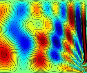
  $mn$-sums portrayed in panels (
 $c$) of figures 1–4. Appendix C.1 accounts for the fan-like structures on the right near
  $r=\ell$, while Appendix C.2 identifies the front location on the left, where the waves are attenuated.

Figure 1. The case  $E=10^{-4}$, blocks of
  $E^{-1/2}\chi$-contours at three distinct instants
  $t=N{\rm \pi} /2$ (
 $N=3,7,11$), namely
  $4.72$,
  $11.00$,
  $17.28$, when
  ${\bar \chi }_{{{\textit {MF}}}}$ is maximised (
 ${\bar v}_{{{\textit {MF}}}}\approx 0$). In order, the four panels (
 $a$–
$a$– $d$) within each block (only the first block is labelled) show (
 $a$) the filtered-DNS
  $\chi _{{{\textit {FNS}}}}$; (
 $b$) the analytic solution
  $\chi ^\sim _{{{{\mathfrak {W}}}}}$ from the new
  ${\mathfrak {W}}$-trigger; (
 $c$) again
  $\chi ^\sim _{{{{\mathfrak {W}}}}}$ but, for comparison, at
  $E=0$; (
 $d$) the analytic solution
  $\chi ^\sim _{{{{\mathfrak {E}}}}}$ from the previous
  ${\mathfrak {E}}$-trigger (the
  $z$-range is
  $0\leqslant z\leqslant 1$; colour scale from
  $-0.1$ (blue) to
  $0.1$ (red)).

Figure 2. As in figure 1 but now at  $t=(N+\tfrac 12){\rm \pi} /2$ (
 $N=3,7,11$), namely
  $5.50$,
  $11.79$,
  $18.07$, when (
 ${\bar v}_{{{\textit {MF}}}}$ is maximised)
  ${\bar \chi }_{{{\textit {MF}}}}\approx 0$.

Figure 3. As in figure 1, but now  $E^{-1/2}v$-contours for the same instants, when (
 ${\bar \chi }_{{{\textit {MF}}}}$ is maximised)
  ${\bar v}_{{\textit {MF}}}\approx 0$. Each block shows (
 $a$) the filtered-DNS
  $v_{{\textit {FNS}}}$; (
 $b$) the analytic solution
  $v^\sim _{{{{\mathfrak {W}}}}}$ from the new
  ${\mathfrak {W}}$-trigger; (
 $c$) again
  $v^\sim _{{{{\mathfrak {W}}}}}$ but, for comparison, at
  $E=0$; (
 $d$) the analytic solution
  $v^\sim _{{{{\mathfrak {E}}}}}$ from the previous
  ${\mathfrak {E}}$-trigger (the
  $z$-range is
  $0\leqslant z\leqslant 1$; colour scale from
  $-0.5$ (blue) to
  $0.5$ (red)).


The results of § 3 and Appendix C must, of course, be interpreted within the framework of the limit  $E\downarrow 0$ and as such only describe waves in the mainstream, exterior to all boundary layers. Once the MF boundary layer (A7) has expanded to fill the entire region on the time scale
  $t=O(E^{-1})$, the solution is no longer applicable, so placing an absolute limit on the usefulness of the solution to the range
  $0 < t \ll E^{-1}$. Viscous effects are, however, manifest on the spin-down time
  $t=O(E^{-1/2})$ and even earlier for waves with sufficiently short length scales (internal friction). So, in § 4, we address the small but finite-
 $E$ corrections to the mainstream individual wave amplitudes
  ${\boldsymbol{v}} ^\sim _{mn}$ found previously in § 3 by solving the governing equations with
  $E=0$. Our remit is restricted to finding
  $O(E^{1/2})$ decay rates and frequency perturbations due to internal friction in § 4.1 and accounting for similar corrections due to Ekman layer damping in § 4.3. The transitory nature of the Ekman layers for modes with frequencies close to 2 introduces complications that we accommodate by a composite solution in § 4.2, which we argue gives the required low order accuracy for all
  $t\ll E^{-1}$.
We performed DNS of the spin-down governing equations subject to the complete boundary conditions for various small values of  $E$, which we discuss in § 5. Oruba et al. (Reference Oruba, Soward and Dormy2020) proposed a filtered DNS (referred to as FNS), for which the QG-part
  ${\bar {\boldsymbol{v}} }_{{\textit {{QG}}}}$ of the complete
  ${\boldsymbol{v}} _{{\textit {DNS}}}$ was removed. In § 5.1 we define a new FNS, whereby the mainstream
  $z$-independent MF-part
  ${\bar {\boldsymbol{v}} }_{{\textit {MF}}}$ is also removed (see (5.4)). This has the advantage, over the previous Oruba et al. (Reference Oruba, Soward and Dormy2020) definition, that the resulting FNS in the mainstream, exterior to all boundary layers, may be compared directly, in § 5.2, with the inertial wave solutions of the triggered wave problem formulated in § 2. Comparisons, at
  $E=10^{-4}$,
  $\ell =10$, are presented in figures 1–4. Within the various panels of those figures, we compare the FNS (
 $a$) to the analytic results from our new
  ${\mathfrak {W}}$-trigger (1.30a) for finite
  $E$ (
$E$ ( $b$) and in the
  $E\downarrow 0$ limit (
 $c$), and our previous
  ${\mathfrak {E}}$-trigger (1.29), employed with
  ${\mathfrak {E}}=1$, (
 $d$). In making comparisons with the results of Oruba et al. (Reference Oruba, Soward and Dormy2020), it is important to note that, up to the same order of accuracy achievable by the
  ${\mathfrak {W}}$-trigger, the
  ${\mathfrak {E}}$-trigger is adequately described by the E-trigger (1.30b). Our new
  ${\mathfrak {W}}$-trigger solutions are almost identical to the FNS, whereas our previous
  ${\mathfrak {E}}$-trigger (essentially the E-trigger) exhibits small amplitude and phase defects. The origin of these defects is explained by various analytic comparisons made in § 3.1 and Appendix C. A more quantitative assessment of the relative accuracy of the analytic and FNS results for our
  ${\mathfrak {W}}$-trigger is described in § 5.3.
We conclude with an overview in § 6.
2. The mathematical problem
Our strategy parallels Oruba et al. (Reference Oruba, Soward and Dormy2020). So here we draw on their results by referencing the relevant equations but only sketch the methodology; for a more careful appraisal, the reader is referred to that work and references therein (for a general reference to inertial waves in a container, see Zhang & Liao Reference Zhang and Liao2017).
The essential idea is that the flow  ${\boldsymbol{v}} _{{{\textit {GH}}}}$ (say) between unbounded parallel planes (
 $\ell \to \infty$), whose LT-solution is given by (3.4)–(3.6) of Greenspan & Howard (Reference Greenspan and Howard1963), provides the lowest-order solution to the bounded (
 $\ell$ large but finite) problem. The main point, emphasised in § 1.3, is that outside boundary layers the horizontal components
  ${\bar {\boldsymbol{v}} }_{{{\textit {{QG}}}}\perp }$ and
  ${\bar {\boldsymbol{v}} }_{{{\textit {MF}}}\perp }$ of both the QG and MF-flow contributions (for
  $\ell \to \infty$), that together comprise
  ${\boldsymbol{v}} _{{{\textit {GH}}}\perp }$ (see (2.1b)), are
  $z$-independent; the small axial components
  ${\bar w}_{{\textit {{QG}}}}$,
  ${\bar w}_{{\textit {MF}}}$ and their sum
  ${\bar w}_{{{\textit {GH}}}}$ are, of course, all linear in
  $z$. However, the failure of the radial velocities
  ${\bar u}_{{\textit {{QG}}}}=(r/\ell ){\bar {\mathfrak {u}}}_{{\textit {{QG}}}}$ and
  ${\bar u}_{{\textit {MF}}}=(r/\ell ){\bar {\mathfrak {u}}}_{{\textit {MF}}}$, both of
  $O(E^{1/2})$, to meet the requirement
  ${\bar u}(\ell ,t)=0$ triggers a further inertial wave response
  $E^{1/2}{\boldsymbol{v}} ^\sim$ (previously written
  $E^{1/2}{\boldsymbol{v}} ^{wave}$ by Oruba et al. Reference Oruba, Soward and Dormy2020). As we are only interested in
  ${\boldsymbol{v}} ^\sim$ outside the Ekman layer (both steady and transient) and sidewall boundary layers, we ignore those boundary layers and write
 \begin{equation} {\boldsymbol{v}}\approx{\bar {\boldsymbol{v}}}_{{{\textit{GH}}}}+E^{1/2}{\boldsymbol{v}}^\sim, \quad {\bar {\boldsymbol{v}}}_{{{\textit{GH}}}}={\bar {\boldsymbol{v}}}_{{{\textit{{QG}}}}}+{\bar {\boldsymbol{v}}}_{{{\textit{MF}}}}. \end{equation}
Our objective is to determine  ${\boldsymbol{v}} ^\sim$ obtained subject to the
  ${\mathfrak {W}}$-trigger boundary condition
 \begin{equation} u^\sim={-}{\mathfrak{U}}(t)={-}\tfrac12{\mathfrak{W}}(t) \quad \mbox{at} \ r=\ell \ (0 < z\leqslant 1) \end{equation}
(see (1.30a)), with a sink of opposite strength at  $z=0$ to ensure that
  $\int _0^1u^\sim \,{\mathrm d} z=0$. It is important to note that the radial flow
  ${\bar u}_{{{\textit {GH}}}}$ differs from the trigger flow
  $(r/\ell ){\bar {\mathfrak {u}}}_{{{{\mathfrak {W}}}}}$, for reasons explained in § 1.3.
Throughout this section we drop the superscript ‘ $\sim$’ and write
  ${\boldsymbol{v}} =[u,v,w]$ (
![]() ). With
). With  $w=r^{-1}\partial (r\chi )/\partial r$ (1.5d), the inertial wave problem is: solve
 \begin{gather} \displaystyle\frac{\partial{v}}{\partial{t}}+2u=E\left(\nabla^2-r^{{-}2}\right)v,\quad u={-}\displaystyle\frac{\partial{\chi}}{\partial{z}}, \end{gather}
 \begin{gather} \displaystyle\frac{\partial{\gamma}}{\partial{t}} -2\dfrac{\partial{v}}{\partial{z}} = E\left(\nabla^2-r^{{-}2}\right)\gamma,\quad \gamma={-}\left(\nabla^2-r^{{-}2}\right)\chi \end{gather}
((2.3a,c) are the azimuthal equations of momentum, vorticity respectively) subject to the initial ( $t=0$) conditions
 \begin{equation} v = 0,\quad \gamma=0, \end{equation}
and for  $t\geqslant 0$ the reduced boundary conditions
 \begin{gather} r\chi=0\quad \mbox{at}\ r=0\ (0 < z\leqslant 1), \end{gather}
 \begin{gather}r\chi=\tfrac12\ell (z-1)\,{\mathfrak{W}}(t)\quad \mbox{at}\ r=\ell\ (0 < z\leqslant 1), \end{gather}
 \begin{gather}\chi=0\quad \mbox{at}\ z=0,1 \ (0 < r < \ell), \end{gather}
in which the stress boundary conditions, appearing in (5.2) below, have been ignored.
2.1. The $z$-Fourier series

We seek  $z$-Fourier series solutions of the form
 \begin{equation} \left[\begin{array}{@{}c@{}} \chi \\ v \end{array}\right]={-}\sum_{m=1}^\infty\displaystyle\frac{({-}1)^m}{m {\rm \pi}} \left[\begin{array}{@{}c@{}} {\tilde \chi}_m(r,t)\sin\left(m{\rm \pi} (z-1)\right) \\ {\tilde{v}}_m(r,t)\cos\left(m{\rm \pi} (z-1)\right) \end{array}\right] \end{equation}
for which (2.5b), noting
 \begin{equation} \frac12 (z-1) ={-}\sum_{m=1}^\infty\displaystyle\frac{({-}1)^m}{m{\rm \pi}}\sin(m{\rm \pi} (z-1)) \quad (0 < z\leqslant 1), \end{equation}
leads to the boundary condition
 \begin{equation} r{\tilde \chi}_m=\ell {\mathfrak{W}}(t) \quad \mbox{at} \ r=\ell. \end{equation}
The LT-solution obtained from ( ${O}$: 2.16
 $a$), following the change
  ${\hat {\mathfrak {E}}}(p)\mapsto {\hat {\mathfrak {W}}}(p)$, is
 \begin{equation} \left[\begin{array}{@{}c@{}} {\hat {\tilde \chi}}_m \\ {\hat {\tilde{v}}}_m \end{array}\right]= \left[\begin{array}{@{}c@{}} 1 \\ 2m{\rm \pi}/{\mathfrak{p}} \end{array}\right]{\hat {\mathfrak{W}}}(p) \displaystyle\frac{{\mathrm J}_1\left(m{\rm \pi} qr\right)}{{\mathrm J}_1\left(m{\rm \pi} q\ell\right)}. \end{equation}
 Here,  ${\mathrm J}_1$ is the Bessel function, while the functions
  ${\mathfrak {p}}={\mathfrak {p}}(p)$ and
  $q=q({\mathfrak {p}})= q({\mathfrak {p}}(p))$ are determined by the dispersion relation (
 ${O}$: 2.17
 $a$–
$a$– $d$), which gives them as the solutions of
 \begin{equation} \left.\begin{array}{r@{}} {\mathfrak{p}}^2={-}4\left/\left(q^2+1\right)\!,\right.\\ {\mathfrak{p}}=p+(q^2+1){\mathsf{d}}_m \end{array} \right\} \ \Longleftrightarrow\ \left\{\begin{array}{@{}l} q^2+1={-}4/{\mathfrak{p}}^2,\\ p={\mathfrak{p}}+4{\mathsf{d}}_m/{\mathfrak{p}}^2, \end{array}\right. \end{equation}
where
 \begin{equation} {\mathsf{d}}_m=E(m{\rm \pi})^2. \end{equation}
 In terms of the Bessel function of imaginary argument  ${\mathrm I}_1$, the initial behaviour
 \begin{equation} {\tilde \chi}_m\approx\displaystyle\frac{8t^{3/2}}{3\sqrt{\rm \pi}}\,\displaystyle\frac{{\mathrm I}_1\left(m{\rm \pi} r\right)}{{\mathrm I}_1\left(m{\rm \pi} \ell\right)}\quad (t\ll 1) \end{equation}
is recovered on expanding the integrand of the inverse-LT  ${\mathcal {L}}^{-1}\{{\hat {\tilde \chi }}_m\}$ of
  ${\hat {\tilde \chi }}_m$ defined by (2.9a) under the limit
  $p\to \infty$, for which
  $q\to {\mathrm i}$ (see (2.9c)) and noting that
  ${\mathfrak {W}}(t)\approx 8t^{3/2}/(3\sqrt {\rm \pi})$ for
  $t\ll 1$ (see (1.13a,c)). The initial response (2.10),
  $\propto t^{3/2}$, is ‘softer’ than the impulsive response (
 ${O}$: 2.9
 $c$) to the
  ${\mathfrak {E}}$-trigger.
For  $t>0$ the LT-inversion of (2.9a) involves consideration of the contributions from various poles, which include the zeros of
  ${\mathrm J}_1(m{\rm \pi} q\ell )$, as well as the cuts at
  $p=\pm 2{\mathrm i}$ exhibited by
  ${\hat {\mathfrak {W}}}(p)$. Since we have omitted the stress boundary conditions at
  $r=\ell$, following Oruba et al. (Reference Oruba, Soward and Dormy2020), we disregard the shear layer responses, both QG and ageostrophic, abutting the outer boundary
  $r=\ell$ linked to the poles
  $p=0$ (in
  ${\hat {\mathfrak {W}}}(p)$) and
  ${\mathfrak {p}}=0$ (in the factor
  ${\mathfrak {p}}^{-1}$ of the expression for
  ${\hat {\tilde {v}}}_m$). Their proper treatment using the full boundary conditions (5.2) was undertaken by Oruba et al. (Reference Oruba, Soward and Dormy2017).
To understand the nature of the triggered waves, we begin by focusing attention on the remaining set  $\daleth$ of poles
  $p=p_{mn}$,
  $p^*_{mn}$ (the superscript ‘
 $*$’ denotes the complex conjugate) identified by
 \begin{equation} q=q_{mn}={j_n}/({m{\rm \pi}\ell})\ (>0), \end{equation}
determined by the real zeros  $j_n$ of
  ${\mathrm J}_1(m{\rm \pi} q \ell )$ (i.e.
  ${\mathrm J}_1(\kern1.5pt j_n)=0$). In turn, they define
 \begin{gather} {\mathfrak{p}}_{mn}={\mathrm i}\omega_{mn},\quad \omega_{mn}={2}/\sqrt{q_{mn}^2+1}, \end{gather}
 \begin{gather} p_{mn}={\mathrm i}\omega_{mn}-d_{mn},\quad d_{mn}=4{\mathsf{d}}_m/\omega_{mn}^2, \end{gather}
and, following the differentiation of  $p={\mathfrak {p}}+4{\mathsf{d}}_m/{\mathfrak {p}}^2$ (2.9c), they determine the value
 \begin{equation} \left[\displaystyle\frac{{\mathfrak{p}}}{p}\displaystyle\frac{{\mathrm d}{p}}{{\mathrm d}{{\mathfrak{p}}}}\right]_{{\mathfrak{p}}={\mathfrak{p}}_{mn}}= \displaystyle\frac{{\mathrm i}\omega_{mn}+2d_{mn}}{{\mathrm i}\omega_{mn}-d_{mn}} \quad \mbox{at} \ p=p_{mn}, \end{equation}
needed to evaluate pole residues in § 4.1 below. From (2.12b), we may generate
 \begin{gather} \varphi_{mn}=\sqrt{1-(\omega_{mn}/2)^2}=\cos (2\alpha_{mn}), \end{gather}
 \begin{gather}\tfrac12\omega_{mn}=\sqrt{1-\varphi_{mn}^2}=\sin(2\alpha_{mn}), \end{gather}
 \begin{gather}q_{mn}=2\varphi_{mn}/\omega_{mn}=\cot(2\alpha_{mn}), \end{gather}
cf.  $\varphi _{mn}$ with
  $\varphi _\pm$ in (C8b) in Appendix C.1 below. The role of the aforementioned cuts re-emerges in (2.19) below.
Our disregard of the QG-response linked to the poles  $p=0$ and
  ${\mathfrak {p}}=0$ has consequences on the boundary values (2.8) of individual triggered waves, which actually satisfy
 \begin{equation} r{\tilde \chi}_m=\ell {\mathfrak{W}}_{{{\textit{MF}}}}(t) \quad \mbox{at} \ r=\ell, \end{equation}
i.e. the oscillatory waves cannot exhibit the steady features of the E-trigger  $\ell \,{\mathfrak {W}}_{{{{E}}}}$ constituent (1.30b) (a curiosity noted and explained in the last paragraph of § 2.3 of Oruba et al. (Reference Oruba, Soward and Dormy2020), in connection with the
  ${\mathfrak {E}}$-trigger).
2.2. The $r$-Fourier–Bessel series

As in Oruba et al. (Reference Oruba, Soward and Dormy2020), we take advantage of the Fourier–Bessel series expansion
 \begin{equation} \displaystyle\frac{{\mathrm J}_1(m{\rm \pi} q r)}{{\mathrm J}_1(m{\rm \pi} q l)}={-} \dfrac12\sum_{n=1}^\infty\dfrac{q_{mn}^2}{\omega_{mn}^{{-}2}+{\mathfrak{p}}^{{-}2}} \, \displaystyle\frac{{\mathrm J}_1(\kern1.5pt j_nr/\ell)}{j_n{\mathrm J}_0(\kern1.5pt j_n)} \quad \mbox{on} \ 0\leqslant r < \ell, \end{equation}
which follows from ( ${O}$: A3) on noting that (2.9c), (2.12b) together imply
  $q_{mn}^2-q^2=4(\omega _{mn}^{-2}+{\mathfrak {p}}^{-2})$. So we write
 \begin{equation} \left[\begin{array}{@{}c@{}} {\tilde \chi}_m \\ {\tilde{v}}_m \end{array}\right] =\sum_{n=1}^\infty \left[\begin{array}{@{}c@{}} {\mathring\chi}^{\mathsf{d}}_{mn} \\ {\mathring v}^{\mathsf{d}}_{mn} \end{array}\right]\displaystyle\frac{{\mathrm J}_1(\kern1.5pt j_nr/\ell)}{j_n{\mathrm J}_0(\kern1.5pt j_n)} \quad \mbox{on} \ 0\leqslant r < \ell. \end{equation}
Here, the superscript ‘ ${\mathsf{d}}$’ distinguishes our general
  ${\mathsf{d}}_m(=E(m{\rm \pi} )^2)\not =0$ (2.9d) usage from the
  ${\mathsf{d}}_m\downarrow 0$ limit considered in the following § 3, where the superscript ‘
 ${\mathsf{d}}$’ will be omitted. It follows that the LT of (2.16a) is determined via
 \begin{equation} \left[\begin{array}{@{}c@{}} \widehat{{\mathring\chi}_{mn}^{\mathsf{d}}} \\ \widehat{{\mathring v}_{mn}^{\mathsf{d}}} \end{array}\right]={-}2\varphi^2_{mn} \left[\begin{array}{@{}c@{}} {\mathfrak{p}} \\ 2m{\rm \pi} \end{array}\right] \displaystyle\frac{{\mathfrak{p}}\,{\hat {\mathfrak{W}}}(p)}{{\mathfrak{p}}^2+\omega_{mn}^2} \end{equation}
on substitution of  $q_{mn}=2\varphi _{mn}/\omega _{mn}$ (2.13c) into (2.15). An unfortunate feature of the Fourier–Bessel series expansion (2.15) is that it necessarily fails at
  $r=\ell$, where each eigenfunction
  ${\mathrm J}_1(\kern1.5pt j_nr/\ell )$ vanishes. So it is not possible for (2.16a) to satisfy the reduced boundary condition
  ${\tilde \chi }_m(\ell ,t)={\mathfrak {W}}_{{\textit {MF}}}(t)$ (2.14) except in the limiting sense
  $r\uparrow \ell$. That such a limit is achievable is exemplified by the early time inverse-LT (2.10) of (2.9a).
We express the inverse-LT of (2.16b) as
 \begin{equation} \left[\begin{array}{@{}c@{}} {\mathring\chi}^{{\mathsf{d}}}_{mn} \\ {\mathring v}^{{\mathsf{d}}}_{mn} \end{array}\right]={-}{\mathcal{L}}^{{-}1}\left\{\varphi^2_{mn} \left[\begin{array}{@{}c@{}} {\mathfrak{p}} \\ 2m{\rm \pi} \end{array}\right]\displaystyle\frac{{\hat {\mathfrak{W}}}(p)}{{\mathfrak{p}}-{\mathrm i}\omega_{mn}} \right\}+\mbox{c.c.}, \end{equation}
where ‘c.c.’ denotes complex conjugate. A further reduction of the LT  $\widehat {\,{\mathring v}_{mn}^{\mathsf{d}}}$, exhibited by the right-hand side of (2.17), is possible upon using the partial fraction decomposition
 \begin{equation} \displaystyle\frac{1}{{\mathfrak{p}}-{\mathrm i}\omega_{mn}}=\displaystyle\frac{1}{{\mathrm i}\omega_{mn}}\left[\displaystyle\frac{{\mathfrak{p}}}{{\mathfrak{p}}-{\mathrm i}\omega_{mn}}-1\right]. \end{equation}
The contribution to the inverse-LT  ${\mathcal {L}}^{-1}\{\widehat {\,{\mathring v}_{mn}^{\mathsf{d}}}\}$ from the second term
  $-1/({\mathrm i}\omega _{mn})$ is pure imaginary and so when added to its complex conjugate vanishes leaving
 \begin{equation} \left[\begin{array}{@{}c@{}} {\mathring\chi}^{\mathsf{d}}_{mn} \\ {\mathring v}^{\mathsf{d}}_{mn} \end{array}\right] =\varphi^2_{mn}\left[\begin{array}{@{}c@{}} -1\\ 2 {\mathrm i} m{\rm \pi}/\omega_{mn} \end{array}\right]{\mathfrak{W}}^{{\mathsf{d}}}_{mn}(t)+\mbox{c.c.}, \end{equation}
where  ${\mathfrak {W}}^{{\mathsf{d}}}_{mn}(t)$ has LT
 \begin{equation} {\hat {\mathfrak{W}}}^{{\mathsf{d}}}_{mn}(p)=\displaystyle\frac{{\mathfrak{p}}{\hat {\mathfrak{W}}}(p)}{{\mathfrak{p}}-{\mathrm i}\omega_{mn}}. \end{equation}
The  ${\mathfrak {W}}^{{\mathsf{d}}}_{mn}$-notation is motivated by the property
  ${\mathfrak {W}}^{{\mathsf{d}}}_{mn}(t)={\mathfrak {W}}(t)$, when
  $\omega _{mn}=0$. So employing
 ![]() (1.13c), we write
(1.13c), we write
 \begin{equation} {\mathfrak{W}}^{{\mathsf{d}}}_{mn}(t)=\sum_{{\pm}}\left\{{\mathfrak{W}}_{mn}^{{{\mathsf{d}}}\pm}(t)\right\}, \end{equation}
where  ${\mathfrak {W}}^{{{\mathsf{d}}}\pm }(t)$ has LT
 \begin{equation} {\hat {\mathfrak{W}}}^{{{\mathsf{d}}}\pm}_{mn}(p)=\displaystyle\frac{{\mathfrak{p}}{\hat {\mathfrak{W}}}^\pm(p)}{{\mathfrak{p}}-{\mathrm i}\omega_{mn}}=\displaystyle\frac{\pm{\mathrm i}\,{\mathfrak{p}}}{p(p\pm 2{\mathrm i})^{1/2}({\mathfrak{p}}-{\mathrm i}\omega_{mn})} \end{equation}
on use of (1.12b).
We must stress that our use of the  ${\mathring \chi }_{mn}$,
  ${\mathring v}_{mn}$ notation, although similar in spirit to Oruba et al. (Reference Oruba, Soward and Dormy2020), differs in detail. For, whereas the factor
  ${\mathfrak {F}}_{mn}=q_{mn}^2\omega _{mn}^2/2=2\varphi ^2_{mn}$ appears multiplying
  $[{\mathring \chi }_{mn}, {\mathring v}_{mn}]$ in (
 ${O}$: 2.23
 $a$), we have removed it from (2.16a), including it instead in (2.16b) (cf. (
 ${O}$: 2.23
 $b$)).
3. The inviscid limit, $E\downarrow 0$, $d_{mn}=0$


We investigate the response (2.19a) in the  $E\downarrow 0$ limit, for which
  ${\mathfrak {p}}=p$ and
  ${\hat {\mathfrak {W}}}^{{\mathsf{d}}\pm }_{mn}(p)$, defined by (2.19d), reduces to
 \begin{equation} {\hat {\mathfrak{W}}}^{{\pm}}_{mn}(p)=\displaystyle\frac{\pm{\mathrm i}}{(p\pm 2{\mathrm i})^{1/2}(p-{\mathrm i}\omega_{mn})}=\left(\displaystyle\frac{2}{{ \boldsymbol{\varpi}}_{mn}^\pm}\right)^{3/2}\,{\hat {\mathfrak{W}}}^{{\pm}}\left(\displaystyle\frac{2}{{ \boldsymbol{\varpi}}_{mn}^\pm}(p-{\mathrm i}\omega_{mn})\right), \end{equation}
with inverse
 \begin{align} &={\mathfrak{P}}^\pm_{mn}\left[{\mathrm{S}}(T^{{\pm}}_{mn})\pm{\mathrm i}{\mathrm C}(T^{{\pm}}_{mn})\right]\exp\left({\mathrm i}\omega_{mn}t\right), \end{align}
in which we have used (1.12b), (1.13) and introduced
We note that the above is a simple adaption of the § 1.2.2 result (1.31), following the change of variables  ${\mathrm i} E^{1/2}\sigma \mapsto \omega _{m,n}$ and
  $2\aleph ^{\pm }\mapsto {\boldsymbol {\varpi }}_{mn}^\pm$.
For  $[{\mathring \chi }^{\mathsf{d}}_{mn}, {\mathring v}^{{\mathsf{d}}}_{mn}]$, substitution of (3.1c) into (2.19a,c) yields the value
 \begin{equation} \left[\begin{array}{@{}c@{}} {\mathring\chi}_{mn} \\ {\mathring v}_{mn} \end{array}\right]={-}2\varphi_{mn}^2\left[\begin{array}{@{}c@{}} \left({\mathcal{C}}_{mn}(t)\cos(\omega_{mn}t) +{\mathcal{S}}_{mn}(t)\sin(\omega_{mn}t)\right)\\ (2m{\rm \pi}/\omega_{mn}) \left({\mathcal{C}}_{mn}(t)\sin(\omega_{mn}t) -{\mathcal{S}}_{mn}(t)\cos(\omega_{mn}t)\right)\end{array}\right], \end{equation}
where
 \begin{equation} \left[{\mathcal{C}}_{mn}(t), {\mathcal{S}}_{mn}(t)\right]=\sum_{{\pm}}\left\{{\mathfrak{P}}^\pm_{mn}\left[{\mathrm{S}}(T^{{\pm}}_{mn}), \mp {\mathrm C}(T^{{\pm}}_{mn})\right]\right\}. \end{equation}
Hence, the complete  $E\downarrow 0$ version of the solution (2.6) is determined by (2.16a) with
  $[{\mathring \chi }^{\mathsf{d}}_{mn}, {\mathring v}^{\mathsf{d}}_{mn}]$ given by (3.2a).
This analytic  ${\mathfrak {W}}$-trigger solution has been estimated numerically (by truncating the sums involved). The result is shown on the twelve panels (
 $c$) of figures 1–4, at instants when the solution is well developed. It differs significantly from the approximate (or reduced)
  ${\mathfrak {E}}({\approx }\textrm {E}$)-trigger solution of Oruba et al. (Reference Oruba, Soward and Dormy2020) illustrated in (
 $d$). For, as a comparison of panels (c,d) shows, the addition of the MF-trigger to form the complete
  ${\mathfrak {W}}(=\textrm {E}+{\textrm {MF}})$-trigger corrects the phase issue apparent when only the
  ${\mathfrak {E}}$-trigger is used. To understand how the correction is achieved, we need to consider the large time asymptotic behaviour of the solution, at which stage the wave mechanisms are identifiable. To that end, the
  $E\downarrow 0$ value
 ![]() of
of  ${\mathfrak {W}}^{{\mathsf{d}}}_{mn}(t)$, given by (3.1b,c), is usefully partitioned into the pole- and cut-contributions of (3.1a).
3.1. The pole part, $\daleth$

On consideration of the explicit form for  ${\hat {\mathfrak {W}}}^{\pm }_{mn}(p)$, given (3.1a) the residue at the pole
  $p={\mathrm i}\omega _{mn}$ is determined from (3.1b), noting that
  ${\mathfrak {W}}^\pm _{{{E}}}=(\pm {\mathrm i}/2)^{1/2}$ (1.15b), as
 \begin{align} {\mathfrak{W}}^\daleth_{mn}(t)&=\left[({\mathrm i}/{\boldsymbol{\varpi}}_{mn}^+)^{1/2}+(-{\mathrm i}/{\boldsymbol{\varpi}}_{mn}^-)^{1/2}\right] \exp\left({\mathrm i}\omega_{mn}t\right) \end{align}
 \begin{align} &=\varphi_{mn}^{{-}1}\exp\left({\mathrm i}\omega_{mn}t-\alpha_{mn}\right), \end{align}
in which we have introduced  $\alpha _{mn}$ via the relation
 \begin{equation} 2\varphi_{mn}=\sqrt{{\boldsymbol{\varpi}}^+_{mn}{\boldsymbol{\varpi}}^-_{mn}}=2\cos (2\alpha_{mn}) \end{equation}
(recall (2.13a) and (3.1d)). The result (3.3b) may be checked by squaring both right-hand sides of (3.3a,b) and noting (2.13b), (3.3c). Substitution of (3.3b) into (2.19a) determines
 \begin{equation} \left[\begin{array}{@{}c@{}} {\mathring\chi}^\daleth_{mn} \\ {\mathring v}^\daleth_{mn} \end{array}\right]={-}2\varphi_{mn} \left[\begin{array}{@{}c@{}} \cos (\omega_{mn}t-\alpha_{mn})\\ (2m{\rm \pi}/\omega_{mn}) \sin(\omega_{mn}t-\alpha_{mn}) \end{array}\right], \quad \left\{\begin{array}{@{}l} 1>\varphi_{mn}>0,\\ 0<\alpha_{mn}<{\rm \pi}/4. \end{array}\right. \end{equation}
Cederlöf (Reference Cederlöf1988) solved this normal mode problem but from a different perspective. At first sight his method appears different to ours, because driving stems directly from the transient Ekman pumping  ${\mathfrak {W}}(t)$ (1.10) (see his (5.21) in which the LT-form
  ${\tilde {F}}(s)$ is essentially our
  ${\hat {\mathfrak {W}}}(p)$) and not from the boundary condition at
  $r=\ell$. Nevertheless, after appropriate variable changes, his solution (5.25) follows directly from (3.3a) via (2.19a), (2.16a). He does not, however, introduce the instructive phase angles
  $\alpha _{mn}$.
It is interesting to compare the above pole response  ${\mathring \chi }_{mn}^{\daleth }=-2\varphi _{mn}\cos (\omega _{mn}t-\alpha _{mn})$ to our
  ${\mathfrak {W}}$-trigger (1.30a), with the corresponding
  ${\mathfrak {E}}$-trigger (1.29) response, which from (
 ${O}$: 4.2
 $a$) is
  ${\mathring \chi }_{mn}^{\daleth {\mathfrak {E}}}=-\tfrac 12 q_{mn}^2\omega _{mn}^2\cos (\omega _{mn}t)=-2\varphi ^2_{mn}\cos (\omega _{mn}t)$. The responses differ by a factor
  $\varphi _{mn}$ but coincide when
  $\varphi _{mn}=1 \ (\alpha _{mn}=0)$. That is the QG-limit
  $\omega _{mn}\downarrow 0$, which occurs as
  $q_{mn}=j_n/(m{\rm \pi} \ell )\to \infty$, namely the short radial-
 $r$ length scale limit (
 $\kern1.5pt j_n\gg 1$). As the frequency
  $\omega _{mn}$ increases,
  $\varphi _{mn}$ decreases (
 $\alpha _{mn}$ increases) in concert. Accordingly, relative to the
  ${\mathfrak {E}}$-trigger response
  ${\mathring \chi }_{mn}^{\daleth {\mathfrak {E}}}$, the phase shifted (
 $\alpha _{mn}\not =0$)
  ${\mathfrak {W}}$-trigger response
  ${\mathring \chi }_{mn}^{\daleth }$ increases in amplitude by a factor
  $1/\varphi _{mn}$. The increasing trend of the phase shift and mode amplitude terminates as
  $\varphi _{mn}\downarrow 0$ (
 $\alpha _{mn}\uparrow {\rm \pi}/4$). That is the MF-limit
  $\omega _{mn}\uparrow 2$, which occurs as
  $q_{mn}\downarrow 0$, namely, the short axial-
 $z$ length scale limit, which is of ever decreasing magnitude
 \begin{equation} \left[\begin{array}{@{}c@{}} {\mathring\chi}^\daleth_{mn} \\ {\mathring v}^\daleth_{mn} \end{array}\right]\approx{-} 2\sqrt{{\boldsymbol{\varpi}}^-_{mn}}\left[\begin{array}{r} \cos (2t-{\rm \pi}/4)\\ m{\rm \pi} \sin(2t-{\rm \pi}/4) \end{array}\right], \quad \mbox{as}\ {\boldsymbol{\varpi}}^-_{mn} \downarrow 0, \end{equation}
with  ${\mathring \chi }^{\daleth }_{mn}$ yet large compared to
  ${\mathring \chi }_{mn}^{\daleth {\mathfrak {E}}}$ by the factor
  $\varphi _{mn}^{-1}\approx 1/\sqrt {{\boldsymbol {\varpi }}^-_{mn}}$. Both the phase shift and increased amplitude of the
  $m=1$ mode are evident in the well-developed solution sufficiently far from the outer boundary
  $r=\ell$ in
  ${\mathfrak {W}}$-panels (
 $c$) of figures 1–4, when compared to the
  ${\mathfrak {E}}$-panels (
 $d$), albeit at
  $E=10^{-4}$.
3.2. The cut part, $\leftrightarrows$

The remaining cut contribution  ${\mathfrak {W}}_{mn}(t)-{\mathfrak {W}}^\daleth _{mn}(t)$ is
 \begin{equation} {\mathfrak{W}}^\leftrightarrows_{mn}(t)=\sum_{{\pm}}\left\{{\mathfrak{W}}^{\leftrightarrows\pm}_{mn}(t)\right\}, \end{equation}
where the results (3.1b) give
 \begin{align} &={-}{\mathfrak{P}}^\pm_{mn}[f(T^{{\pm}}_{mn})\pm{\mathrm i} g(T^{{\pm}}_{mn})]\exp(\mp2{\mathrm i} t) \end{align}
on application of (1.17b,c), noting  $T^{\pm }_{mn}=({\boldsymbol {\varpi }}^{\pm }_{mn}T/2)^{1/2}$ (3.1f) (but cf. (3.1c)). The large
  $T^{\pm }_{mn}$ asymptotic behaviour
  $f(T^{\pm }_{mn})\approx ({\rm \pi} T^{\pm }_{mn})^{-1/2}$,
  $g(T^{\pm }_{mn})\approx 0$ (see (A4a)) determines
 \begin{equation} {\mathfrak{W}}^{\leftrightarrows}_{mn}(t)\approx{-}\varphi^{{-}2}_{mn}({\rm \pi} t)^{{-}1/2}\left[\cos (2t)-\tfrac12 {\mathrm i}\omega_{mn}\sin(2t)\right] \quad \mbox{for} \ T^{{\pm}}_{mn}\gg 1. \end{equation}
Substitution into (2.19a) yields
 \begin{equation} \left[\begin{array}{@{}c@{}} {\mathring\chi}^\leftrightarrows_{mn} \\ {\mathring v}^\leftrightarrows_{mn} \end{array}\right] \approx\displaystyle\frac{2}{\sqrt{{\rm \pi} t}} \left[\begin{array}{r} \cos (2t)\\ m{\rm \pi} \sin(2t) \end{array}\right], \end{equation}
similar to (3.5) except for the phase shift  ${\rm \pi} /4$ but notably smaller by a factor
  $({\rm \pi} {\boldsymbol {\varpi }}^-_{mn}t)^{-1/2}\approx \sqrt {2}/({\rm \pi} T^-_{mn})$ whenever
  $T^-_{mn}\gg 1$.
The simplicity of (3.8) suggests the possibility of constructing from it the large  $t$ asymptotic form of the cut solution. On use of the identity
 \begin{equation} \displaystyle\frac{r}{2\ell}={-}\sum_{n=1}^\infty\,\displaystyle\frac{{\mathrm J}_1(\kern1.5pt j_nr/\ell)}{j_n{\mathrm J}_0(\kern1.5pt j_n)}, \end{equation}
determined from the  $q\to 0$ limit of (
 ${O}$: A3), substitution of (3.8) into the
  $r$-Fourier–Bessel series (2.16a) yields
 \begin{equation} \left[\begin{array}{@{}c@{}} {\tilde \chi}_m^{\leftrightarrows} \\ {\tilde{v}}_m^{\leftrightarrows} \end{array}\right] \approx{-}\displaystyle\frac{r}{\ell}\displaystyle\frac{1}{\sqrt{{\rm \pi} t}} \left[\begin{array}{@{}c@{}} \cos(2t) \\ m{\rm \pi}\sin (2t) \end{array}\right]\quad \mbox{as}\ t\to\infty. \end{equation}
Substitution into the  $z$-Fourier series (2.6), noting (1.19b), determines
 \begin{equation} \left[\begin{array}{@{}c@{}} \chi^{\leftrightarrows} \\ v^{\leftrightarrows} \end{array}\right]\approx{-} \displaystyle\frac{1}{\sqrt{4{\rm \pi} t}}\,\displaystyle\frac{r}{\ell}\left[\begin{array}{@{}c@{}} (z-1) \cos(2t) \\ \sin (2t) \end{array}\right]\approx{-}E^{{-}1/2} \left[\begin{array}{@{}c@{}} {\bar\chi}_{{{\textit{MF}}}} \\ {\bar v}_{{{\textit{MF}}}} \end{array}\right]\quad (z>0) \end{equation}
 The result (3.10) raises disturbing issues. It suggests that the dominant cut contribution determines a flow contribution of the same size (but opposite in sign) as the original Greenspan and Howard MF-flow responsible for the MF-trigger. However, because of the discontinuous nature of the Fourier series for  $(z-1)$ and
  $1$ at
  $z=0$ and the Fourier–Bessel series for
  $r$ at
  $r=\ell$, the series have to reach extremely large values of
  $m$ and
  $n$ to achieve convergence. This is an issue because of the large
  $T^{-}_{mn}$ requirement
  $t\gg 1/{\boldsymbol {\varpi }}^-_{mn}=1/(2-\omega _{mn})$ (see (3.1d) and (3.7)). So at any finite
  $t$ (however large), it is unclear how good the approximation is. Certainly at the values of
  $t$, for which results are reported here, some evidence of an MF-contribution from the cut was evident in tests (not illustrated). However, surprisingly a similar MF-contribution from the poles was also found (again not illustrated), which when combined with the cut-contribution led to their cancellation, i.e. there is no evidence of an MF-contribution in panels (
 $c$) of figures 1–4, or for that matter in panels (
 $a$), (
 $b$) of those figures at small but finite
  $E$. The large time MF-issues raised provide a focal point for our discussion of the
  $\ell \gg 1$ limit in Appendix C, which explains the curious cancellation evident in the aforementioned numerical results (not illustrated).
Remarkably, the ‘method of images’ approach of Appendix C.1, identifies immediately the main cut contribution (3.10) that prompted our concerns, via the MF-part  $-{\mathfrak {U}}_{{\textit {MF}}}(t)$ of the very first term
  $-{\mathfrak {U}}(t)$ on the right-hand side of (C1a). The role of the poles is subtler, because the estimate
  $|{\mathring \chi }^\daleth _{mn}| \sim T_{mn} |{\mathring \chi }^\leftrightarrows _{mn}|$ below (3.8) suggests that the pole contribution will be even bigger. However, the second term on the right-hand side of final result (C6b) demonstrates that wave interference must occur reducing the accumulated pole effect to exactly that from the cuts. The fact, that
  $-{\mathfrak {U}}_{{\textit {MF}}}(t)=O(t^{-1/2})$ is indeed the dominant cut contribution, is established by (C6c), which shows the remainder to be even smaller
  $O(t^{-1})$ for
  $t\gg 1$.
An alternative perspective is gleaned from the steepest descent results of Appendix C.2, which for  $t\gg 1$ identify two wave families
  ${\tilde \chi }_\pm$ (C7). The triggered MF-wave
  ${\tilde \chi }_-$, characterised by (C10c,d,f), is only pertinent close to the outer boundary
  $r=\ell$. There, it remains small compared to the low frequency mode
  ${\tilde \chi }_+$, characterised by (C10a,b,e). Of even greater importance is the identification, in the last paragraph of Appendix C.2, of a wave front at which the
  ${\tilde \chi }_\pm$-waves merge and beyond which the waves are evanescent, a feature clearly visible in figures 1–4.
4. Small but finite $0 < E \ll 1$

The amplitude of the  $E\downarrow 0$ wave-solution, derived in the previous § 3, takes no account of its viscous damping. Such consideration is needed to achieve comparison with the direct numerical simulations, which are necessarily undertaken at finite
  $E$. In this section, we rectify that omission.
The complete inversion of the LT (2.19d) to obtain  ${\mathfrak {W}}^{{\mathsf{d}}\pm }_{mn}(t)$ in the small
  $E$ limit is formidable. So in this section we simply outline an approximate method that suffices for our purpose. To that end we note that the solution may be partitioned as
 \begin{equation} {\mathfrak{W}}^{{\mathsf{d}}\pm}_{mn}(t)={\mathfrak{W}}^{{\mathsf{d}}\pm\daleth}_{mn}(t)+{\mathfrak{W}}^{{\mathsf{d}}\pm\leftrightarrows}_{mn}(t), \end{equation}
where  ${\mathfrak {W}}^{{\mathsf{d}}\pm \daleth }_{mn}$ and
  ${\mathfrak {W}}^{{\mathsf{d}}\pm \leftrightarrows }_{mn}$ are the pole and cut contributions to the inverse-LT of (2.19d).
4.1. Pole solution
The pole contribution is determined from (2.19d) by the residue
 \begin{equation} {\mathfrak{W}}^{{\mathsf{d}}\daleth\pm}_{mn}(t)=\left[\displaystyle\frac{\pm{\mathrm i}}{(p\pm 2{\mathrm i})^{1/2}}\,\displaystyle\frac{{\mathfrak{p}}}{p}\displaystyle\frac{{\mathrm d}{p}}{{\mathrm d}{{\mathfrak{p}}}}\exp(pt)\right]_{{\mathfrak{p}}={\mathrm i}\omega_{mn}} \end{equation}
of the inverse-LT at  $p=p_{mn}={\mathrm i}\omega _{mn}-d_{mn}$ (2.12c,d), corresponding to
  ${\mathfrak {p}}={\mathrm i}\omega _{mn}$ (2.12a). On use of the expression (2.12e) for
  $[({\mathfrak {p}}/p)({\mathrm d} p/{\mathrm d}{\mathfrak {p}})]_{{\mathfrak {p}}={\mathrm i}\omega _{mn}}$ and noting from (3.1d) that
  $p_{mn}\pm 2{\mathrm i}=\pm {\mathrm i}{\boldsymbol {\varpi }}^{\pm }_{mn}-d_{mn}$, the residue (4.2) becomes
 \begin{equation} {\mathfrak{W}}^{{\mathsf{d}}\daleth\pm}_{mn}(t)=\tfrac12 (1 \pm{\mathrm i})\, {\mathfrak{P}}^{{\mathsf{d}}\pm}_{mn}\exp\left({\mathrm i}\omega_{mn}t-d_{mn}t\right)\!, \end{equation}
where
 \begin{equation} {\mathfrak{P}}^{{\mathsf{d}}\pm}_{mn}=\left(\displaystyle\frac{2}{{\boldsymbol{\varpi}}^{{\pm}}_{mn}\pm {\mathrm i} d_{mn}}\right)^{1/2}\displaystyle\frac{\omega_{mn}-2{\mathrm i} d_{mn}}{\omega_{mn}+{\mathrm i} d_{mn}}, \end{equation}
in which  $\mbox {Re}\{({\boldsymbol {\varpi }}^{\pm }_{mn}\pm {\mathrm i} d_{mn})^{1/2}\}>0$ as required by analytic continuation on increasing
  $d_{mn}$ from zero. The decay rate
  $d_{mn}=4E(m{\rm \pi} )^2/\omega _{mn}^2$ (see (2.9d), (2.12d)) is a consequence of internal friction (identified by the first term in (4.5) of Zhang & Liao Reference Zhang and Liao2008).
4.2. Composite solution
To obtain an approximate solution of the full problem, we make the ansatz
 \begin{equation} {\mathfrak{W}}^{{\mathsf{d}}\pm}_{mn}(t)={\mathfrak{P}}^{{\mathsf{d}}\pm}_{mn}\,{\mathfrak{W}}^{{\pm}}\left({\boldsymbol{\varpi}}^{{\pm}}_{mn}t\big/2\right) \exp\left({\mathrm i}\omega_{mn}t-d_{mn}t\right)\!, \end{equation}
which has the properties
 \begin{equation} {\mathfrak{W}}^{{\mathsf{d}}\pm}_{mn}(t)\to \left\{\begin{array}{@{}ll} {\mathfrak{W}}^{{\pm}}_{mn}(t) \quad & \mbox{as} \ d_{mn}\to 0,\\ {\mathfrak{W}}^{{\mathsf{d}}\daleth\pm}_{mn}(t) & \mbox{as}\ T^{{\pm}}_{mn}\to \infty. \end{array}\right. \end{equation}
The former limit (4.4b) is a simple consequence of the fact that ![]() , as
, as  $d_{mn}\downarrow 0$, so recovering the
  $E\downarrow 0$ result (3.1b). The latter limit (4.4c) applies because
  ${\mathfrak {W}}^{\pm }({\boldsymbol {\varpi }}^{\pm }_{mn}t\big /2)\to {\mathfrak {W}}_{{{E}}}^\pm =\tfrac 12 (1 \pm {\mathrm i})$ (1.15b), as
  $T^{\pm }_{mn}\to \infty$, leaving the pole contribution (4.3), i.e. the remaining cut contribution
  ${\mathfrak {W}}^{{\mathsf{d}}\pm \leftrightarrows }_{mn}(t)$ is assumed negligible in this limit.
Our construction of the composite (4.4a) is in much the same spirit as Greenspan and Howards’ unbounded flow composite  ${\bar {\mathfrak {u}}}_{{\textit {GH}}}(t)$ (1.31b), i.e. neither is a true asymptotic formula, but instead both capture the dominant flow characteristics.
4.3. Ekman layer damping
Consistent with our construction of the composite (4.4a), we implement Ekman damping by replacing the exponential  $\exp ({\mathrm i}\omega _{mn}t-d_{mn}t)$ with
 \begin{equation} \exp\left[{\mathrm i}\left(\omega_{mn}+\omega^E_{mn}\right)t-\left(d_{mn}+d^E_{mn}\right)t\right], \end{equation}
where the frequency and damping increments  $\omega ^E_{mn}$ and
  $d^E_{mn}$ adopted are those for pure inertial waves, given by (
 ${O}$: 2.25) (also Kerswell & Barenghi Reference Kerswell and Barenghi1995; Zhang & Liao Reference Zhang and Liao2008). The increments have the form
 \begin{equation} \left[\begin{array}{@{}c@{}} d^E_{mn}\\ \omega^E_{mn} \end{array}\right]=\sqrt{\displaystyle\frac{E}{2}}\,\varphi_{mn} \left[\begin{array}{@{}c@{}} (2-\varphi_{mn})\sqrt{1+\varphi_{mn}} \\ (2+\varphi_{mn})\sqrt{1-\varphi_{mn}} \end{array}\right], \end{equation}
where  $\varphi _{mn}=\tfrac 12\sqrt {{\boldsymbol {\varpi }}^+_{mn}{\boldsymbol {\varpi }}^-_{mn}}=\sqrt {1-(\omega _{mn}/2)^2}$ (see (3.3c)), as can be verified by squaring both sets of expressions for
  $d^E_{mn}$ and
  $\omega ^E_{mn}$, given by (4.5b) and (
 ${O}$: 2.25
 $b$).
$b$).
The oscillatory Ekman layer adjacent to  $z=0$, frequency
  $\omega _{mn}$, has a double layer structure of respective widths
 \begin{equation} \varDelta_{mn}^\pm={\mathfrak{P}}_{mn}^\pm\sqrt{E}, \end{equation}
where  ${\mathfrak {P}}_{mn}^\pm =\sqrt {2/{\boldsymbol {\varpi }}_{mn}^\pm }$ (3.1e) (cf., e.g. Kerswell & Barenghi Reference Kerswell and Barenghi1995, (2.8)). The two widths are readily identifiable on setting
  $p=2{\mathrm i} \omega _{mn}$ in the exponential
 ![]() of the LT-solution (1.12a) for
of the LT-solution (1.12a) for  ${\mathfrak {z}}^\pm (z,t)$. In the geostrophic limit
  $\omega _{mn}=0$ (
 ${\mathfrak {P}}_{mn}^\pm =1$), the steady Ekman layer width
  $\varDelta _{{{E}}}=\sqrt {E}$ is recovered. The width
 \begin{equation} \varDelta^-_{mn}=\sqrt{Et_{mn}} \quad \mbox{with} \ t_{mn}=({\mathfrak{P}}^-_{mn})^2=2/{\boldsymbol{\varpi}}_{mn}^->0, \end{equation}
of the broader layer increases indefinitely as  ${\boldsymbol {\varpi }}_{mn}^-\downarrow 0$ (
 ${\mathfrak {P}}^-_{mn}\to \infty$), i.e.
  $\omega _{mn}\uparrow 2$. So the boundary layers of inertial modes, possessing frequencies close to
  $2$, fill the entire gap
  $0\leqslant z\leqslant 1$ of the layer.
In addition to the MF matters associated particularly with the final steady state just discussed, there are also delicate issues concerning how those states are reached. The key feature of the transient evolution of inertial modes is their expanding viscous boundary layer width  $\varDelta (t)=\sqrt {Et}$ (1.14). It eventually splits into two parts, each of which ceases to grow at time
  $t=t^\pm _{mn}$ that solves
  $\varDelta (t)=\varDelta ^\pm _{mn}$. Since
  $\varDelta ^-_{mn}>\varDelta ^+_{mn}$ with
  $t^-_{mn}>t^+_{mn}$, the splitting occurs at
  $t=t_{mn}^+$, at which the thinner reaches its final width
  $\varDelta ^+_{mn}$. For
  $t>t^+_{mn}$, the thicker broadens until terminating with width
  $\varDelta ^-_{mn}$ at
  $t=t^-_{mn}$. Furthermore, whenever
  $t^-_{mn}\gg 1$, this time may be longer than the times reached in our numerical investigations. In any event, when either
  $\varDelta ^-_{mn}=O(1)$ or
  $1\ll t \leqslant O(t^-_{mn})$, formula (4.5b) for
  $d^E_{mn}$ and
  $\omega ^E_{mn}$ ceases to apply. Nevertheless, since (4.5b) predicts
  $d^E_{mn}\to 0$ and
  $\omega ^E_{mn}\to 0$ as
  $|\omega _{mn}|\uparrow 2$ (
 $\varphi _{mn}\downarrow 0$), their use in that limit, although inappropriate, ought to be harmless.
The defects, just described are of exactly the same nature as the failure of the Greenspan & Howard (Reference Greenspan and Howard1963) LT-solution (1.26) near the cut points  $p=\pm 2{\mathrm i}$, elucidated in the antepenultimate paragraph of § 1.2.2 which ends with the definition (1.30) of the
  ${\mathfrak {W}}$-trigger. In short, the failure of both the trigger and the waves pertain to boundary layers that expand to fill the entire domain, and as such are two sides of the same coin.
Our appraisal of the situation indicates that it is impossible to produce asymptotic ( $0 < E \ll 1$) results that are justifiable in all space or for all time. As explained, our proposed solution (4.4a) modified by (4.5a), namely
 \begin{equation} {\mathfrak{W}}^{E{\mathsf{d}}\pm}_{mn}(t)={\mathfrak{P}}^{{\mathsf{d}}\pm}_{mn}\,{\mathfrak{W}}^{{\pm}}\left(\left.{\boldsymbol{\varpi}}^{{\pm}}_{mn}t\right/2\right) \exp\left[{\mathrm i}\left(\omega_{mn}+\omega^E_{mn}\right)t-\left(d_{mn}+d^E_{mn}\right)t\right], \end{equation}
is weakest for disturbances with  $\omega _{mn}\approx 2$. Furthermore, in view of the approximate nature of the
  ${\mathfrak {W}}$-trigger (1.30), nothing is gained by using the primitive form
  ${\mathfrak {W}}^{{\mathsf{d}}\pm }_{mn}(t)$ of the damped (internal friction only) wave solution defined by its LT (2.19). We, therefore, simply adopt (4.8). Indeed, despite many approximations, our guiding consideration is to maintain accuracy compatible with our
  ${\mathfrak {W}}$-trigger assumption. The very tight comparisons with DNS reported in the following § 5 fully endorse this strategy.
5. The filtered DNS (FNS) velocity
In § ${O}$:
 $3$ we presented results from the spin-down obtained by performing DNS of the full, yet linearised, governing equations (2.3) subject to the initial conditions
 \begin{equation} {v/r}=1,\quad {r\chi}=0\quad\mbox{everywhere at}\ t=0, \end{equation}
and boundary conditions
 \begin{gather} {r \chi}=\displaystyle\frac{\partial{{(v/r)}}}{\partial{r}}=\displaystyle\frac{\partial{{w}}}{\partial{r}}=0\quad \mbox{at}\ r=0\ \mbox{and}\ \ell\quad (0 < z < 1), \end{gather}
 \begin{gather}{r \chi}=\displaystyle\frac{\partial{{(r \chi)}}}{\partial{z}}={v/r}=0\quad \mbox{at}\ z=0\quad (0 < r < \ell), \end{gather}
 \begin{gather}{r \chi}=\displaystyle\frac{\partial{^2{(r \chi)}}}{\partial{z^2}}=\displaystyle\frac{\partial{{(v/r)}}}{\partial{z}}=0\quad \mbox{at} \ z=1\quad (0 < r < \ell), \end{gather}
i.e. the bottom plate is rigid (5.2b), whereas the top and side boundaries are stress free (5.2a,c). From those results, Oruba et al. (Reference Oruba, Soward and Dormy2020) described how asymptotics valid for  $E\ll 1$, could be used to remove the QG-part
  ${\bar {\boldsymbol{v}} }_{{\textit {{QG}}}}$ of the flow external to all boundary layers, leaving what they referred to as the filtered DNS (FNS, §O:3.1). From an analytic point of view, that remaining FNS is the sum of the underlying MF-flow
  ${\bar {\boldsymbol{v}} }_{{\textit {MF}}}$, described in §§ 1.2.1, 1.2.2, together with the wave part
  $E^{1/2}{\boldsymbol{v}} ^\sim$ triggered at the outer boundary. To simplify matters, only the
  ${\mathfrak {E}}$-triggered wave
  $E^{1/2}{\boldsymbol{v}} ^\sim _{{{{\mathfrak {E}}}}} (=E^{1/2}{\boldsymbol{v}} ^{\mathrm {wave}}$ in (
 ${O}$: 2.1)) was considered by Oruba et al. (Reference Oruba, Soward and Dormy2020). Here, we improve on that simplification by considering the flow more faithfully described by
  $E^{1/2}{\boldsymbol{v}} ^\sim _{{{{\mathfrak {W}}}}}\ (\mbox {i.e.}\ E^{1/2}{\boldsymbol{v}} ^\sim$ in (2.1a)).
5.1. Our new FNS
We consider the decompositions
 \begin{gather} {\boldsymbol{v}}={\boldsymbol{v}}_{{\textit{{QG}}}}+{\boldsymbol{v}}_{{{\textit{MF}}}}+E^{1/2}{\boldsymbol{v}}^\sim, \end{gather}
 \begin{gather}{\boldsymbol{v}}_{{\perp}}={\bar {\boldsymbol{v}}}_{{{\textit{{QG}}}}\perp}+{\boldsymbol{v}}^{{{\varDelta}}}_{{{\textit{{QG}}}}\perp}+{\bar {\boldsymbol{v}}}_{{{\textit{MF}}}\perp}+ {\boldsymbol{v}}^{{{\varDelta}}}_{{{\textit{MF}}}\perp}+E^{1/2}{\boldsymbol{v}}^\sim_{{\perp}} \end{gather}
of the entire velocity  ${\boldsymbol{v}}$ and the horizontal velocity
  ${\boldsymbol{v}} _{\perp }$. Note that there are also ageostrophic sidewall boundary layer contributions adjacent to
  $r=\ell$, ignored in (5.3a,b). The
  $z$-average of (5.3b) yields
 \begin{equation} \langle{\boldsymbol{v}}_{{\perp}}\rangle=\langle{\boldsymbol{v}}_{{{\textit{{QG}}}}\perp}\rangle+\langle{\boldsymbol{v}}_{{{\textit{MF}}}\perp}\rangle+O(E), \end{equation}
where the wave Ekman layer contribution  $\langle {\boldsymbol{v}} ^\sim _{\perp } \rangle =O(E^{1/2})$ is included in the
  $O(E)$ error. As the filter only pertains to the flow outside all boundary layers, we are only interested in the contribution
  ${\bar {\boldsymbol{v}} }_{{{\textit {{QG}}}}\perp }+{\bar {\boldsymbol{v}} }_{{{\textit {MF}}}\perp }+E^{1/2}{\boldsymbol{v}} ^\sim _{\perp }$ to (5.3b). Oruba et al. (Reference Oruba, Soward and Dormy2020) filtered the DNS by simply removing the
  $z$-independent QG-contribution
  ${\bar {\boldsymbol{v}} }_{{{\textit {{QG}}}}\perp }$. However, a more useful filter is obtained by removing, in addition, the MF-contribution
  ${\bar {\boldsymbol{v}} }_{{{\textit {MF}}}\perp }$, which like
  ${\bar {\boldsymbol{v}} }_{{{\textit {{QG}}}}\perp }$ is
  $z$-independent. By this devise we are left with our new filtered horizontal velocity
 \begin{equation} {\boldsymbol{v}}_{{{\textit{FNS}}}\perp}=E^{{-}1/2}\left({\boldsymbol{v}}_{{{\textit{DNS}}}\perp}-{\bar {\boldsymbol{v}}}_{{{\textit{{QG}}}}\perp}-{\bar {\boldsymbol{v}}}_{{{\textit{MF}}}\perp}\right). \end{equation}
To evaluate our new filter (5.4), we assume that the needed features of the MF-part of the DNS are
 \begin{gather} E^{{-}1/2}{\bar {\boldsymbol{v}}}_{{{\textit{MF}}}\perp}\approx(r/\ell)[{\mathfrak{U}}_{{{\textit{MF}}}}, {\mathfrak{V}}_{{{\textit{MF}}}}+{\mathfrak{R}}_{{{\textit{MF}}}}], \end{gather}
 \begin{gather}E^{{-}1/2}\langle{\boldsymbol{v}}_{{{\textit{MF}}}\perp}\rangle\approx(r/\ell)[0,{\mathfrak{R}}_{{{\textit{MF}}}}], \end{gather}
as given by the analytic results (1.21) and (1.24). Thus, with  ${\boldsymbol{v}} _{{{\textit {MF}}}}$ assumed known, we remove it from both sides of (5.3a) and so obtain
  ${\boldsymbol{v}} _{{{\textit {DNS}}}\perp }-{\boldsymbol{v}} _{{{\textit {MF}}}\perp }={\boldsymbol{v}} _{{{\textit {{QG}}}}\perp }+ E^{1/2}{\boldsymbol{v}} ^\sim _{\perp }$ instead of (5.3b). Then, as in Oruba et al. (Reference Oruba, Soward and Dormy2020), we use the recipe implicit in (
 ${O}$: 3.4) and (
 ${O}$: 3.7
 $a$) to relate
  ${\bar v}_{{\textit {{QG}}}}$ and
  ${\bar u}_{{\textit {{QG}}}}$ to
  $\langle v_{{\textit {{QG}}}} \rangle$
 \begin{equation} E^{{-}1/2}{\bar {\boldsymbol{v}}}_{{{\textit{{QG}}}}\perp}\approx\mu^{{-}1}\left[\tfrac12\sigma,E^{{-}1/2}\right]\langle v_{{\textit{{QG}}}} \rangle, \end{equation}
where  $\sigma \approx 1+\tfrac 34 E^{1/2}$ (1.28e),
  $\mu \approx 1-\tfrac 12 E^{1/2}$. Next, (5.3c) determines
 \begin{equation} \langle v_{{{\textit{{QG}}}}}\rangle\,\approx\,\langle v_{{{\textit{DNS}}}}\rangle-\langle v_{{{\textit{MF}}}}\rangle\approx\langle v_{{{\textit{DNS}}}}\rangle-E^{1/2}(r/\ell){\mathfrak{R}}_{{{\textit{MF}}}}, \end{equation}
on use of (5.5b). Substitution of  $E^{-1/2}{\bar {\boldsymbol{v}} }_{{{\textit {MF}}}\perp }$ (5.5a) and
  $E^{-1/2}{\bar {\boldsymbol{v}} }_{{{\textit {{QG}}}}\perp }$ (5.6a,b) into (5.4) then provides an explicit representation of
  ${\boldsymbol{v}} _{{{\textit {FNS}}}\perp }$ in terms of
  ${\boldsymbol{v}} _{{{\textit {DNS}}}\perp }$ and known analytic results. Finally we note that
 \begin{equation} \chi_{{{\textit{FNS}}}}= E^{{-}1/2} \chi_{{{\textit{DNS}}}}-E^{{-}1/2}({\bar u}_{{\textit{{QG}}}}+{\bar u}_{{\textit{MF}}})(1-z), \end{equation}
in which  $E^{-1/2}{\bar u}_{{\textit {{QG}}}}\approx \tfrac 12(\sigma /\mu )\langle v_{{\textit {{QG}}}} \rangle$ (see (5.6a)) and
  $E^{-1/2}{\bar u}_{{\textit {MF}}}\approx (r/\ell ){\mathfrak {U}}_{{{\textit {MF}}}}$ (see (5.5a)).
Following the neglect of  $\langle v^\sim \rangle =O(E^{1/2})$ and other similar approximations such as the reliability of the trigger itself (see e.g. (1.32)), we expect the filter values
  $\chi _{{{\textit {FNS}}}}$ (5.7) and
  $v_{{{\textit {FNS}}}}$ (the azimuthal component of (5.4)) to agree with the analytic predictions for
  $\chi _{{{{\mathfrak {W}}}}}^\sim$ and
  $v_{{{{\mathfrak {W}}}}}^\sim$, with
  $O(E^{1/2})$ error.
5.2. FNS results
For  $E=10^{-4}$, FNS solutions (using the new filter described above in § 5.1) are compared to those obtained using the analytic results of §§ 3, 4 in figures 1–4. All figures are arranged in three blocks (each consisting of four panels (a–d)) corresponding to different time instants. We adopt the times employed in figures
  ${O}$:
 $1$–
$1$– ${O}$:
 $4$, close to which either
  $\chi _{{\textit {MF}}}$ or
  $v_{{\textit {MF}}}$ take their stationary values (i.e. the zeros of the time derivative of
  ${\mathfrak {U}}_{{\textit {MF}}}$ or
  ${\mathfrak {V}}_{{\textit {MF}}}$ given by (1.18a)). As
  $t\to \infty$, they coincide with the vanishing of the corresponding asymptotic forms (A5). Although, having filtered out the MF-contribution, those instants are no longer special, we limit our attention to them in order to facilitate comparison of our current
  ${\mathfrak {W}}$-trigger results with the earlier
  ${\mathfrak {E}}$-trigger results displayed in figures
  ${O}$:
 $1$–
$1$– ${O}$:
 $4$, albeit for the larger
  $E=10^{-3}$. On the one hand, the effects of dissipation are less evident in our
  $E=10^{-4}$ figures 1–4. On the other hand and related, our new displays pertain to a very early stage of the spin-down process, i.e. short compared to the QG spin-down time
  $O(E^{-1/2})=O(100)$ for
  $E=10^{-4}$. As our filter removes the QG flow, the time stage is largely irrelevant to the filter output.
The FNS values for the  ${\mathfrak {W}}$-trigger are portrayed in panel (
 $a$) of every block. The dark region at the bottom of those panels reflects the Ekman layer (thin and very dark) and the expanding MF shear layer, when present in figures 1, 4 (thicker with some contours visible), that the filter does not remove. There is also an ageostrophic
  $E^{1/3}$-sidewall Stewartson layer adjacent to the outer
  $r=\ell$ boundary that the filter does not remove either. Further, it is important to realise that, when the MF-contributions are negligible as in figures 2, 3, the new filter (5.4) is essentially the same as the previous filter. Our
  ${\mathfrak {W}}$-triggered wave solution portrayed in panel (
 $b$) of every block is based on the Ekman layer damped composite solution (4.8). Outside the aforesaid boundary layers, the agreement with panels (
 $a$) is remarkable. For comparison, we show
  ${\mathfrak {E}}$-triggered wave solution, based on the results of Oruba et al. (Reference Oruba, Soward and Dormy2020) (previously portrayed for
  $E=10^{-3}$, but see the following paragraph) in panel (
 $d$). Although the
  ${\mathfrak {E}}$-results identify all the major wave processes involved, the
  ${\mathfrak {E}}$-results are clearly found wanting, and, unlike the robust
  ${\mathfrak {W}}$-results, do not capture the FNS solution in detail.
The comparisons just described are all for  $E=10^{-4}$. We can see the effect of changing
  $E$ from
  $10^{-3}$ to
  $10^{-4}$ by comparing the FNS, IW (
 $\textrm {MF}+$‘wave’) panels (b), (c) (etc.) of figures
  ${O}$:
 $2$,
$2$,  ${O}$:
 $3$ with our FNS, waves(
 $^\sim$) panels (a), (b) (all blocks) of figures 2, 3, because at the instants (with no MF-contribution) chosen the two filters coincide, as do the IW and waves.
In panels ( $c$) of figures 1–4, we portray
  $E=0$ results obtained by use of (3.1b) (equivalently (3.1c)), namely the
  $E=0$ version of (4.8). Their comparison with panels (
 $b$) shows how the small dissipation damps the waves. The large scale features are weakly damped, whereas the small scale structures near
  $r=\ell$ are strongly damped. Their further comparison of panels (
 $b$) with (
 $a$) shows how well our damping ansatz (4.5) works outside the ageostrophic
  $E^{1/3}$-sidewall layer, and particularly close to it, where the
  $E=0$ panels (
 $c$) show considerable fan structure, the smoothing of which by dissipation is captured accurately. We mention also that figures
  ${O}$:
 $6$,
$6$,  ${O}$:
 $7$ show the
  $E=0$
$E=0$  ${\mathfrak {E}}$-response that correspond to the
  ${\mathfrak {W}}$-results portrayed in panels (
 $c$) of figures 2, 3. Direct correspondence is not easy. Still, as the
  $E=10^{-4}$ results are very similar to the
  $E=0$ results except near
  $r=\ell$, the major differences are simply illustrated in figures 1–4 by comparing the
  ${\mathfrak {W}}$-wave results panels (
 $b$) with the
  ${\mathfrak {E}}$-wave results panels (
 $d$).
$d$).
Other than the effects of damping, all other features are explained by the  $E=0$ analysis of § 3. There we identify the main modification of the
  ${\mathfrak {E}}$-wave results of Oruba et al. (Reference Oruba, Soward and Dormy2020) that lead to our present
  ${\mathfrak {W}}$-wave results and so do not repeat them here.
5.3. Quantitative tests
In this subsection, our objective is to assess quantitatively how well the FNS is approximated by the analytic  ${\mathfrak {W}}$-triggered wave results on decreasing
  $E$. To achieve that goal, we analyse the results for
  $v_{{\textit {FNS}}}(E)$ and
  $v_{{{{\mathfrak {W}}}}}^\sim (E)$ portrayed in the final
  $t=18.07$ block of panels (
 $a$)–(
 $c$) in figure 4, extending the values of
  $E$ considered to include
  $E=10^{-n}$,
  $n=3$, 4, 5, 6. In figures 5 and 6, various quantitative tests are made over the range
  $5 \leqslant r\leqslant 9$ of significant wave activity, yet outside the
  $E^{1/3}$-sidewall layer abutting the outer boundary
  $r=10$. The height
  $z=0.8$ chosen for the horizontal cross-sections is
(i) sufficiently far above the lower boundary
$z=0$ to avoid possible corruption of the results by the tail of the lower $\sqrt {Et}$-MF boundary layer; and(ii) well inside the upper cells, illustrated in figure 4, in order to capture substantial azimuthal
$v$-wave motion.


Figure 5. Horizontal cross-sections of  $v$-field measures over the range
  $5\leqslant r\leqslant 9$ at
  $z=0.8$, at
  $t=18.07$. (
 $a$) Shows the linearly interpolated values
  $v^{{lerp}}_{{{\textit {FNS}}}}(E_1,E_2)$ (5.10) that estimate
  $v_{{{\textit {FNS}}}}(0)$;
  $(E_1,E_2)=(10^{-3},10^{-4})$ (red),
  $(10^{-4},10^{-5})$ (green),
  $(10^{-5},10^{-6})$ (blue). (
 $b$) Shows the discrepancy
  $[\![ v ]\!](E)$ (5.11) between the FNS and
  ${\mathfrak {W}}$-trigger solution;
  $E= 10^{-3}$ (red),
  $10^{-4}$ (green),
  $10^{-5}$ (blue),
  $10^{-6}$ (light blue).

Figure 6. Horizontal cross-sections at  $t=18.07$, as in figure 5, showing the
  $E^{-1/2}$-scaled (
 $a$) increment of
  $v_{{{{\mathfrak {W}}}}}^\sim (E)$, namely
  $\delta v_{{{{\mathfrak {W}}}}}^\sim (E)/E^{1/2}$ (5.12a); (
 $b$) increment of
  $v_{{{\textit {FNS}}}}(E)$, namely
  $\delta v_{{{\textit {FNS}}}}(E)/E^{1/2}$ (5.12b); (
 $c$) difference
  $[\![ v ]\!](E)$, namely
  $[\delta v_{{{\textit {FNS}}}}(E)-\delta v_{{{{\mathfrak {W}}}}}^\sim (E)]/E^{1/2}$ (5.12c) (illustrated previously in figure 5(
 $b$), albeit without the
  $E^{-1/2}$-scaling).
The reason for avoiding both the  $E^{1/3}$-sidewall and
  $\sqrt {Et}$-MF boundary layers is that our filter cannot resolve them.
Of particular interest is the  $E\downarrow 0$ value of the horizontal FNS-velocity
  ${\boldsymbol{v}} _{{{\textit {FNS}}}\perp }(E)$, which being a measure of
  $E^{1/2}{\boldsymbol{v}} _{{{\textit {FNS}}}\perp }(E)$, is only defined for
  $E>0$. All our estimates suggest that its value is determined analytically by the
  $E=0$ value of
  ${\boldsymbol{v}} ^\sim _{{\mathfrak {W}}\perp }(E)$ determined by the results (3.2a,b) of § 3. So our expectation is that
 \begin{equation} {\boldsymbol{v}}_{{{\textit{FNS}}}\perp}(0)\equiv\lim_{E\downarrow 0}{\boldsymbol{v}}_{{{\textit{FNS}}}\perp}={\boldsymbol{v}}^\sim_{{\mathfrak{W}}\perp}(0). \end{equation}
For  $0 < E \ll 1$, various analytic estimates suggest that exterior to all boundary layers
  ${\boldsymbol{v}} _{{{\textit {FNS}}}\perp }(E)$ and
  ${\boldsymbol{v}} ^\sim _{{\mathfrak {W}}\perp }(E)$ have, at fixed
  $t$, expansions of the form
 \begin{gather} {\boldsymbol{v}}_{{{\textit{FNS}}}\perp}(E)={\boldsymbol{v}}_{{{\textit{FNS}}}\perp}(0)+E^{1/2} {\boldsymbol{v}}_{{{\textit{FNS}}}\perp}^{\prime}+O(E), \end{gather}
 \begin{gather}{\boldsymbol{v}}^\sim_{{\mathfrak{W}}\perp}(E)={\boldsymbol{v}}^\sim_{{\mathfrak{W}}\perp}(0)+E^{1/2} {\boldsymbol{v}}^{{\sim}\prime}_{{\mathfrak{W}}\perp}+O(E), \end{gather}
where the notation  $\bullet ^{\prime }$ is intended to suggest
  ${\mathrm d} \bullet /{\mathrm d} E^{1/2}|_{E\downarrow 0}$. As our filter has
  $O(E^{1/2})$ errors, there is no asymptotic reason for
  ${\boldsymbol{v}} _{{{\textit {FNS}}}\perp }^{\prime }$ and
  ${\boldsymbol{v}} ^{\sim \prime }_{{\mathfrak {W}}\perp }$ to agree. The main purpose of our tests in figures 5 and 6 is to assess the worth of our ansatz (5.9).
As we cannot determine  $v_{{\textit {DNS}}}(0)$ (and hence
  $v_{{\textit {FNS}}}(0)$) other than via the limit
  $E\downarrow 0$, we consider instead its linearly interpolated value
 \begin{equation} v^{{lerp}}_{{{\textit{FNS}}}}(E_1,E_2)\equiv\displaystyle\frac{E_2^{1/2}v_{{\textit{FNS}}}(E_1)-E_1^{1/2}v_{{\textit{FNS}}}(E_2)}{E_2^{1/2}-E_1^{1/2}}, \end{equation}
which we plot in figure 5( $a$) for various pairs
  $(E_1,\,E_2)$. In (5.9), we have been cautious to offer only a two term Maclaurin series. In the unlikely event of the series remaining valid up to the next term
  $O(E)$, it would follow that
  $v^{{lerp}}_{{{\textit {FNS}}}}(E_1,E_2)= v_{{\textit {FNS}}}(0)+ O((E_1E_2)^{1/2})$, and then only for sufficiently small
  $E_1$ and
  $E_2$. Be that as it may, the
  $v^{{lerp}}_{{{\textit {FNS}}}}(E_1,E_2)$ cross-section in figure 5(
 $a$) converges well. The limiting curve
  ${\boldsymbol{v}} ^\sim _{{\mathfrak {W}}\perp }(0)$ is not plotted being indistinguishable to graph plotting accuracy, consistent with our expectation (5.8).
To obtain a measure of the relative sizes of  $v_{{\textit {FNS}}}^{\prime }$ and
  $v^{\sim \prime }_{{{{\mathfrak {W}}}}}$, we plot in figure 5(
 $b$) the difference
 \begin{equation} [\![ v ]\!](E)\equiv v_{{\textit{FNS}}}(E)-v^\sim_{{{{\mathfrak{W}}}}}(E)= E^{1/2}[v_{{\textit{FNS}}}^{\prime}-v^{{\sim}\prime}_{{{{\mathfrak{W}}}}}]+O(E) \end{equation}
with  $O(E)$ error, as estimated by (5.9). Reassuringly,
  $[\![ v ]\!](E)$ decreases with decreasing
  $E$ consistent with the implications of convergence in figure 5(
 $a$), but not very fast. So in figure 6(
 $c$), we plot the scaled value
  $[\![ v ]\!]/E^{1/2}$, which by (5.11) ought to tend to an
  $O(1)$ limit. Instead it shows sign of increasing with decreasing
  $E$. It should be emphasised, however, that we are attempting to identify very small effects. For with
  $v_{{\textit {FNS}}}=O(E^{1/2}v_{{\textit {DNS}}})$,
  $v_{{\textit {FNS}}}^{\prime }=O(E^{1/2}v_{{\textit {DNS}}})$,
  $v^{\sim \prime }_{{{{\mathfrak {W}}}}}=O(E^{1/2}v_{{\textit {DNS}}})$, the relation (5.11) implies that
  $[\![ v ]\!]=O(E v_{{\textit {DNS}}})$, an accuracy which is perhaps hard to achieve from the numerics.
As a further test of the ansatz (5.9) we plot respectively
 \begin{gather} \delta v^\sim_{{\mathfrak{W}}}(E)\equiv v^\sim_{{\mathfrak{W}}}(E)-v^\sim_{{\mathfrak{W}}}(0)=E^{1/2} v_{{\mathfrak{W}}}^{\prime}+O(E), \end{gather}
 \begin{gather}\delta v_{{{\textit{FNS}}}}(E)\equiv v_{{\textit{FNS}}}(E)-v^\sim_{{\mathfrak{W}}}(0)=E^{1/2} v^{\prime}_{{{\textit{FNS}}}} +O(E), \end{gather}
scaled by  $E^{-1/2}$ in figure 6(a,b). There is some evidence that both
  $\delta v^\sim _{{\mathfrak {W}}}(E)/E^{1/2}$ and
  $\delta v_{{{\textit {FNS}}}}(E)/E^{1/2}$ are approaching the proposed respective limiting values
  $v_{{\mathfrak {W}}}^{\prime }$ and
  $v^{\prime }_{{{\textit {FNS}}}}$. To assess this tendency from a slightly different perspective, we plot
  $[\![ v ]\!](E)/E^{1/2}$ (5.11) in figure 6(
 $c$). Being related to (5.12a,b) via
 \begin{equation} [\![ v ]\!](E)=\delta v_{{{\textit{FNS}}}}(E)-\delta v^\sim_{{\mathfrak{W}}}(E), \end{equation}
its small size relative to both  $\delta v^\sim _{{\mathfrak {W}}}(E)$ and
  $\delta v_{{{\textit {FNS}}}}(E)$ is very reassuring, despite lacking evidence of convergence. The lack of convergence may be attributable to the aforementioned numerical error. More seriously, however, the implied presumption that the
  $O(E^{1/2})$ value of
  $[\![ v ]\!](E)=O(E^{1/2})$ defined by (5.11) is meaningful at that order is flawed, because our
  ${\mathfrak {W}}$-trigger (1.30), used to obtain
  $v^\sim _{{{{\mathfrak {W}}}}}(E)$, itself possesses
  $O(E^{1/2})$ errors, as explained in § 1.3. Essentially, the accuracy of our
  ${\mathfrak {W}}$-trigger is strictly limited and what figure 6(
 $c$) attempts to illustrate is beyond the accuracy claimed by our asymptotics. Despite the caveat about figure 6(
 $c$), the quantitative measures in figures 5 and 6, strongly support the convergence of the FNS results as
  $E\downarrow 0$ to the
  $E=0$ analytic results.
6. Concluding remarks
Our present work, when combined with the QG-study of Oruba et al. (Reference Oruba, Soward and Dormy2017), provides a full analytical solution to the problem of the linear time-dependent motion of a rotating fluid in a plane layer including lateral boundaries, pioneered in the seminal article of Greenspan & Howard (Reference Greenspan and Howard1963). A central feature of our study is the elongated aspect ratio of the domain. In a container with  $O(1)$ aspect ratio, inertial wave activity shows little structure and decays rapidly, because waves are quickly reflected at the axis with no time available to create the coherent travelling structures.
The strong inertial wave activity in an elongated domain is likely to have important consequences for the dynamics of large vortices in the atmosphere, such as tropical cyclones. It is indeed quite possible that these waves are associated with the eye-wall replacement (Houze et al. Reference Houze, Chen, Smull, Lee and Bell2007; Fischer, Rogers & Reasor Reference Fischer, Rogers and Reasor2020), a feature that is often observed prior to rapid intensifications. In actual tropical cyclones one can estimate the Ekman number in the range  $10^{-4} < E < 0.2$ (Oruba, Davidson & Dormy Reference Oruba, Davidson and Dormy2018), which is small enough to motivate the asymptotic study presented here. It should be stressed, however, that in actual tropical cyclones, nonlinear effects cannot be a priori neglected and will thus modify the wave dynamics.
To investigate these waves, the simplified  ${\mathfrak {E}}$-trigger (1.29), essentially equivalent to the E-trigger (1.30b), was adopted by Oruba et al. (Reference Oruba, Soward and Dormy2020). The triggered waves
  ${\boldsymbol{v}} ^\sim _{{{{\mathfrak {E}}}}}$ obtained within that framework were adequate to explain the main features of the DNS results. Here, we extend that preliminary study to include the MF-trigger (1.30c), so constructing the
  ${\mathfrak {W}}$-trigger (1.30a). For
  $E=10^{-4}$, we find that the comparisons in figures 1–4 of our
  ${\boldsymbol{v}} ^\sim _{{{{\mathfrak {W}}}}}$ predictions based on the faithful
  ${\mathfrak {W}}$-trigger (
 $b$) with the FNS waves
  ${\boldsymbol{v}} ^\sim _{{\textit {FNS}}}$ (
 $a$) are almost perfect in the mainstream above the Ekman layer adjacent to the lower boundary
  $z=0$ and away from the ageostrophic
  $E^{1/3}$-layer abutting outer boundary
  $r=\ell$. We stress that the comparable
  ${\mathfrak {E}}$-trigger results figures
  ${O}$:
 $1$–
$1$– ${O}$:
 $4$ pertain to the larger value
  $E=10^{-3}$ at which diffusive effects are more evident. Only for
  $E=10^{-4}$ and smaller is viscosity unambiguously suppressed.
Essentially, relative to Oruba et al. (Reference Oruba, Soward and Dormy2020), our  ${\mathfrak {W}}$-trigger not only incorporates the E-trigger but the additional MF-trigger as well. Respectively, they take account of the blocking of
  ${\bar {\mathfrak {u}}}_{{{E}}}=\tfrac 12 E^{1/2}$ (1.30b) and
  ${\bar {\mathfrak {u}}}_{{\textit {MF}}}(t)=\tfrac 12 E^{1/2} {\mathfrak {U}}_{{\textit {MF}}}(t)$ (1.30c). The latter MF-waves are identifiable as such when
  $t\gg 1$ (Greenspan & Howard Reference Greenspan and Howard1963). However, for
  $t\leqslant O(1)$, both
  ${\bar {\mathfrak {u}}}_{{{E}}}$ and
  ${\bar {\mathfrak {u}}}_{{\textit {MF}}}(t)$ are the same size. More strikingly at that early time, the transient Ekman boundary layer flow
  ${\mathfrak {u}}(z,t)$ (see (1.7a)) exhibits a thin but expanding boundary layer width
  $\varDelta (t)=(Et)^{1/2}$. As the steady Ekman layer part
  ${\mathfrak {u}}_{{{E}}}(z)$ (1.16) has width
  $\varDelta _{{{E}}}=E^{1/2}$, the width of the remaining MF boundary layer part
  ${\mathfrak {u}}_{{\textit {MF}}}(z,t)$ is necessarily the same, in order that the boundary layer width of the sum (
 ${\mathfrak {u}}={\mathfrak {u}}_{{{E}}}+{\mathfrak {u}}_{{\textit {MF}}}$) is
  $\varDelta (t)$. That is why we remarked in item (ii
 $b$) (below (1.18)) that ‘for
  $t\leqslant O(1)$, the E(or QG)/MF-partition (1.15)–(1.18) is unhelpful’. Only for
  $t\gg 1$ is the representation (A7) of
  ${\mathfrak {u}}_{{\textit {MF}}}(z,t)$ truly illuminating.
The above considerations imply that  ${\bar {\mathfrak {u}}}_{{{{\mathfrak {E}}}}}(t)$ and
  ${\bar {\mathfrak {u}}}_{{{{\mathfrak {W}}}}}(t)$, which define the
  ${\mathfrak {E}}$- and
  ${\mathfrak {W}}$-triggers, (1.29b) and (1.30a) respectively, are distinctly different for
  $t\leqslant O(1)$, at which stage it is to be expected that the responses to each will also differ. What is surprising is that the difference is not apparent simply at small times but persists, as a comparison of the
  $E\downarrow 0$ analytic
  ${\boldsymbol{v}} _{{{{\mathfrak {W}}}}}^\sim$ and
  ${\boldsymbol{v}} _{{{{\mathfrak {E}}}}}^\sim$ triggered waves, in (c,d) respectively of figures 1–4, shows. On the one hand, that comparison shows that the
  ${\mathfrak {E}}$-trigger results (
 $d$) give a good qualitative description of the wave structure visible in
  ${\boldsymbol{v}} _{{\textit {FNS}}}$ ((
 $a$) for
  $1\gg E>0$). On the other hand,
  ${\boldsymbol{v}} _{{{{\mathfrak {E}}}}}^\sim$ (
 $d$) suffers a systematic phase shift and decreased amplitude relative to the true
  ${\boldsymbol{v}} _{{{{\mathfrak {W}}}}}^\sim$ (
 $c$), i.e. the essential differences between the
  ${\mathfrak {E}}$- and
  ${\mathfrak {W}}$-triggered responses, for
  $t\gg 1$, are manifest by each wave of given frequency
  $\omega _{mn}$ being ‘rung’ with different strength and phase by the respective triggers. In the limiting case
  $E\downarrow 0$, these wave characteristics are identified by the residues of
  ${\hat {\mathfrak {E}}}(p)$ and
  ${\hat {\mathfrak {W}}}(p)$ at the poles
  $p={\mathrm i} \omega _{mn}$, as explained in § 3.1 with the ideas reinforced by the large
  $\ell$ analysis of Appendix C (but see particularly (C7)–(C9) of Appendix C.2). For those reasons alone, our proper consideration of the
  ${\mathfrak {W}}$-trigger has yielded a significant improvement over the simpler analysis of the
  ${\mathfrak {E}}$-trigger presented in Oruba et al. (Reference Oruba, Soward and Dormy2020).
Significantly, although  ${\hat {\mathfrak {E}}}(p)$ only possesses poles,
  ${\hat {\mathfrak {W}}}(p)$ has cut points as well at
  $p=\pm 2{\mathrm i}$. In § 3.2, we showed that the latter are responsible for wave activity primarily of the MF-type, which appears to cancel Greenspan and Howards’ MF-trigger flow. This is an issue, because despite the algebraic decay with time, the MF-trigger flow exists at the times
  $t\,({\gg }1)$ illustrated in figures 1 and 4. They are not visible because our new filter has hidden them. However, if we examine the FNS (old filter) and IW panels of the corresponding figures
  ${O}$:
 $1$ and
  ${O}$:
 $4$, they dominate the wave pattern beyond the triggered wave extent apparent on our new figures 1–4 right up to the axis
  $r=0$. In Appendix C, we resolved this matter by adopting a Cartesian approximation of the geometry based on
  $\ell \gg 1$, which applies for
  $r \gg 1$ up to the outer boundary
  $r=\ell$. The
  $t\gg 1$ analysis of Appendix C.1 gives the surprising result that the poles provide an accumulated MF-contribution that exactly offsets that due to the cuts. The afore mentioned wave extent is explained and quantified using the method of coalescing saddles (see e.g. Kelvin's ship-wave pattern https://dlmf.nist.gov/36.13 application of the method) in Appendix C.2.
The above remarks about figures 1–4 allude to another matter, namely that they pertain to times  $t$ less than the time
  $t_{{axis}}=O(\ell )$ taken for the triggered waves to reach the
  $r=0$ axis. After that time, wave reflection occurs leading to a confused wave pattern. The ratio of
  $t_{{axis}}$ to the spin-down time is thus
  $E^{1/2}\ell$. As we have taken
  $E=10^{-4}$,
  $\ell =10$ in figures 1–4, for which
  $E^{1/2}\ell =10^{-1}$, all those plots correspond to the early spin-down time range
  $1\ll t \ll E^{-1/2}$. Upon restricting our times for plots to less than
  $E^{1/2}\ell$, we need to increase the size of
  $E$ to obtain a
  $t=O(E^{-1/2})$ plot time. Indeed the
  $E=10^{-3}$ value taken in figures
  ${O}$:
 $1$–
$1$– ${O}$:
 $4$ is just adequate for that purpose but seriously reduces the accuracy of the asymptotics. As our objective here has been to identify the waves generated with high precision accuracy, we have refrained from following that tack.
Nevertheless, the comparison in figures 1–4 of triggered wave  ${\boldsymbol{v}} ^\sim _{{{{\mathfrak {W}}}}}$ amplitudes (b) with the FNS
  ${\boldsymbol{v}} _{{\textit {FNS}}}$ amplitudes (a), at the same value of
  $E$, show subtle improvements over the comparison of
  ${\boldsymbol{v}} ^\sim _{{{{\mathfrak {W}}}}}$ as
  $E\downarrow 0$ (c) with
  ${\boldsymbol{v}} _{{\textit {FNS}}}$. That improvement is particularly striking for the
  $\chi$-contours of figures 1 and 2 just outside the ageostrophic
  $E^{1/3}$ Stewartson shear layer where the fan structure (see Appendix C.1), very evident on (c), is smoothed out (perhaps for
  $r\gtrsim 0.95$) on (b) to provide excellent agreement with (
 $a$). In § 5.3 we performed tighter numerical tests on the dependence on
  $E$ in the range
  $0.5\leqslant r\leqslant 0.9$ beyond
  $r\sim 0.95$, where variation with
  $E$ is less dramatic. The results portrayed in figures 5 and 6 provide evidence indicating that our analytic treatment of dissipation effects encapsulated by (4.8), which captures the secular viscous wave decay predicted by (4.5), works extremely well for
  $t\gg 1$.
Of course, a comparison with experimental data would be very rewarding. However, that needs a spin-down experiment (as yet not performed), with a weak forcing to provide a near linear flow, and an elongated aspect ratio, essential to prevent early reflections. It should be stressed again that our work only addresses the linear limit of vanishing Rossby number. Finite Rossby number effects, although interesting, cannot be quantified in this framework, and deserve further study.
Finally, it is worth reflecting on how our asymptotic approach would compare to an analytic solution  ${\boldsymbol{v}} (r,z,t)$ of the governing equations (2.3) subject to the initial (5.1) and boundary (5.2) conditions, as used by the DNS described in § 5. Consider such an LT-solution
  ${\hat {\boldsymbol{v}} }(r,z,p)$. Presumably its LT-inversion simply involves the residues at poles just like those for the unbounded
  $\ell \to \infty$ case given by (3.4), (3.5) of Greenspan & Howard (Reference Greenspan and Howard1963). The poles near
  $p=0$ would define the slow spin-down, while the others would define damped waves, each with distinct spatial structure and decay rate. However, as our objective is to determine the overall structure, that emerges, when
  $t\ll E^{-1}$, on superposing all modes, such an approach is unenlightening for the same reasons that it was abandoned by Greenspan & Howard (Reference Greenspan and Howard1963). The price paid by their asymptotics is the introduction of cuts that do not exist in the original problem. Our approach inherits the consequences of those cuts which are reflected by the character of our
  ${\mathfrak {W}}$-trigger. However, for
  $t\gg 1$, the cut influence decays algebraically with time and a modal structure emerges. What remains are the pole modes with frequencies
  $\omega _{mn}$ (3.4) in § 3.1, which are modified to
  $\omega _{mn}+\omega ^E_{mn}$ and damped by the rates
  $d_{mn}+d^E_{mn}$ given by (4.5) in § 4.3. All the disturbing cut issues evaporate as time proceeds. In short, our asymptotics has correctly identified the persistent (i.e. dominant) inertial waves generated, together with their amplitudes over the spin-down time
  $t=O(E^{-1/2})$.
Declaration of interests
The authors report no conflict of interest.
Appendix A. The transient Ekman MF-layer of § 1.1
The transient Ekman layer problem is outlined in § 2.3 of Greenspan (Reference Greenspan1968). There he provides the solution, (2.3.4), (2.3.5), of the governing equations (2.3.1)–(2.3.3). His function  $F(z,t)$ (2.3.6) is simply our MF-function
  ${\mathrm i}{\mathfrak {z}}^-_{{\textit {MF}}}(z,t)$ (see (1.17a)), more specifically
 \begin{align} {\mathfrak{z}}^\pm_{{\textit{MF}}}&=\displaystyle\frac{\mp{\mathrm i}}{2}\left[\exp[(1\pm{\mathrm i})E^{{-}1/2}z]\,{\mbox{erfc}}\,\left(\displaystyle\frac{z}{\sqrt{4Et}} +(1\pm{\mathrm i})t^{1/2}\right)\right.\nonumber\\ &\quad \left.-\exp[-(1\pm{\mathrm i})E^{{-}1/2}z]\,{\mbox{erfc}}\,\left(-\displaystyle\frac{z}{\sqrt{4Et}}+ (1\pm{\mathrm i})t^{1/2}\right)\right]. \end{align}
Put another way, in the LT-inversion of  ${\hat {\mathfrak {z}}}^\pm$ to obtain
  ${\mathfrak {z}}^\pm ={\mathfrak {z}}^\pm _{{{E}}}+{\mathfrak {z}}^\pm _{{\textit {MF}}}$, the steady E-part
  ${\mathfrak {z}}^\pm _{{{E}}}$ (1.15a) stems from the pole at
  $p=0$, whereas the MF-contributions
  ${\mathfrak {z}}^\pm _{{\textit {MF}}}$ (1.17a) originate from the cut contributions about
  $p=\mp 2{\mathrm i}$.
The formula (A1) is at first sight unenlightening. However, in the  $t\gg 1$ limit for which the E/MF-partition is useful, the result may be interpreted on use of the formula
 \begin{equation} \,{\mbox{erfc}}\,(\zeta)={\mp}{\mathrm i}(1\pm{\mathrm i})\left[f\left(\displaystyle\frac{2\zeta}{(1\pm{\mathrm i})\sqrt{\rm \pi}}\right)\pm{\mathrm i} g\left(\displaystyle\frac{2\zeta}{(1\pm{\mathrm i})\sqrt{\rm \pi}}\right)\right]\exp\left(-\zeta^2\right) \end{equation}
obtained by reorganising (http://dlmf.nist.gov/7.5.E10). Here, the auxiliary functions  $f$,
$f$,  $g$ were introduced in (1.17c) and defined below it. Application of (A2) to (A1), with
  $\zeta$ taking its respective values in the first and second lines, leads to the representation (1.17a) with
 \begin{equation} {\mathfrak{h}}^\pm_{{\textit{MF}}}={-}\tfrac12(1\pm{\mathrm i})\left[\left[f(T+Z^\pm)-f(T-Z^\pm)\right]\pm{\mathrm i}\left[g(T+Z^\pm)-g(T-Z^\pm)\right]\right], \end{equation}
where  $T(t)=\sqrt {4t/{\rm \pi} }$ (1.13b) and
 \begin{equation} Z^\pm=\displaystyle\frac{z}{(1\pm{\mathrm i})\sqrt{{\rm \pi} E t}}. \end{equation}
 Henceforth in this appendix, we restrict attention to the large- $t$ limit, equivalently
 \begin{equation} T\gg 1, \end{equation}
for which (7.12.2/3) of §http://dlmf.nist.gov/7.12.ii give the asymptotic expansions
 \begin{equation} \left[\begin{array}{@{}c@{}} f(T) \\ g(T) \end{array}\right]=\displaystyle\frac{1}{{\rm \pi} T}\left[\begin{array}{@{}c@{}} 1 \\ ({\rm \pi} T^2)^{{-}1} \end{array}\right] [1+O(T^{{-}4})]\approx\displaystyle\frac{1}{\sqrt{4{\rm \pi} t}} \left[\begin{array}{@{}c@{}} 1 \\ (4t)^{{-}1} \end{array}\right]. \end{equation}
Their use in (1.18a) determines
 \begin{equation} \left[\begin{array}{@{}c@{}} {\mathfrak{U}}_{{\textit{MF}}}(t) \\ {\mathfrak{V}}_{{\textit{MF}}}(t) \end{array}\right] \approx\displaystyle\frac{1}{\sqrt{4{\rm \pi} t}} \left[\begin{array}{@{}c@{}} -\cos (2t) \\ \sin(2t) \end{array}\right] \end{equation}
in which we have made the approximations  $f(T)\approx ({\rm \pi} T)^{-1}$ and
  $g(T)\approx 0$.
To identify the MF boundary layer structure defined by  ${\mathfrak {z}}^\pm _{{\textit {MF}}}(z,t)$, we assume that
  $Z^\pm =O(1)$ with the implication that
 \begin{equation} |Z^\pm|\ll T. \end{equation}
Accordingly, a Taylor series expansion of (A3a) determines
 \begin{equation} {\mathfrak{h}}^\pm_{{\textit{MF}}}\approx{-}(1\pm{\mathrm i})Z^\pm f^\prime(T)\approx\displaystyle\frac{z}{4t \sqrt{{\rm \pi} E t}}, \end{equation}
where the prime denotes derivative and  $Z^\pm$ is given by (A3b). Substitution of (A6b) into (1.17a) and use of (1.11a) determines
 \begin{equation} \left[\begin{array}{@{}c@{}} {\mathfrak{u}}_{{\textit{MF}}} \\ {\mathfrak{v}}_{{\textit{MF}}} \end{array}\right]= \frac12\left[\begin{array}{@{}c@{}} {\mathfrak{z}}^+_{{\textit{MF}}}+{\mathfrak{z}}^-_{{\textit{MF}}} \\ ({\mathfrak{z}}^+_{{\textit{MF}}}-{\mathfrak{z}}^-_{{\textit{MF}}})/{\mathrm i} \end{array}\right]\approx\displaystyle\frac{z}{4t \sqrt{{\rm \pi} E t}} \left[\begin{array}{@{}c@{}} \cos(2t) \\ - \sin(2t) \end{array}\right]\exp\left[-\displaystyle\frac{z^2}{4Et}\right]. \end{equation}
Appendix B. The mean azimuthal MF-flow ${\bar {\mathfrak {v}}}_{{\textit {MF}}}(t)$ for $t=O(1)$


After various integrations of (1.23b) by parts, using the integral representation of  ${\mathfrak {U}}_{{{\textit {MF}}}}$ in the first equality of (1.18a), we may write
 \begin{equation} E^{{-}1/2}{\bar {\mathfrak{v}}}_{{{\textit{MF}}}}\approx 2\int_t^\infty{\mathfrak{U}}_{{{\textit{MF}}}}\,{\mathrm d} t={\mathfrak{V}}_{{\textit{MF}}}+{\mathfrak{R}}_{{\textit{MF}}} , \end{equation}
where
 \begin{equation} {\mathfrak{R}}_{{\textit{MF}}}={-}t\left(\displaystyle\frac{{\mathrm d}{{\mathfrak{V}}_{{\textit{MF}}}}}{{\mathrm d}{t}}+2{\mathfrak{U}}_{{\textit{MF}}}\right)-\frac12{\mathfrak{V}}_{{\textit{MF}}}, \end{equation}
in which  ${\mathrm d}{\mathfrak {V}}_{{\textit {MF}}}/{\mathrm d} t=({\rm \pi} t)^{-1/2}\cos (2t)$. Together, they may be employed to establish that the
  $z$-average
  $\langle v_{{\textit {MF}}}\rangle =\langle {\bar v}_{{\textit {MF}}}\rangle +\langle {\mathfrak {v}}_{{\textit {MF}}}^{{{\varDelta }}}\rangle$ of the azimuthal MF-flow is given by
 \begin{equation} (\ell/r)\langle v_{{\textit{MF}}}\rangle\approx{\bar {\mathfrak{v}}}_{{\textit{MF}}} + \int_0^\infty{\mathfrak{v}}_{{\textit{MF}}}^{{{\varDelta}}}\,{\mathrm d} z={\bar {\mathfrak{v}}}_{{\textit{MF}}}-E^{1/2}{\mathfrak{V}}_{{\textit{MF}}}=E^{1/2}{\mathfrak{R}}_{{\textit{MF}}}. \end{equation}
It decays rapidly
 \begin{equation} {\mathfrak{R}}_{{\textit{MF}}}\approx{-}\displaystyle\frac{\cos(2 t)}{8\sqrt{\rm \pi}\, t^{3/2}}=O\left({\mathfrak{V}}_{{{\textit{MF}}}}/t\right), \quad \mbox{for} \ t\gg 1, \end{equation}
showing that  $E^{-1/2}{\bar {\mathfrak {v}}}_{{{\textit {MF}}}}/{\mathfrak {V}}_{{{\textit {MF}}}}\to 1$ as
  $t\to \infty$, which establishes the estimates (1.25).
Appendix C. The Cartesian limit, $\ell = L/H\gg 1$, $\ell -r = O(1)$, for $E\downarrow 0$


In this appendix, to obtain a better understanding of the § 3 results, we implement the  $\ell \gg 1$ asymptotics of §
 ${O}$:4 that approximates the outer cylindrical geometry as Cartesian and approximates the discrete values
  $j_n/\ell$ (see (2.11)) by a continuous wavenumber
  $k$. Thus, Fourier–Bessel sums become Fourier integrals, i.e.
  $\sum _n\mapsto \int {\mathrm d} n$.
C.1. The ‘method of images’
As in § ${O}$:5, we focus attention on the radial velocity
  $u$ expressed in the form
 \begin{equation} u\approx{-}{\mathfrak{U}}(t)+\sum_{-\infty}^\infty{\breve u}_l,\quad {\breve u}_l(x,z,t)={\breve u}(x,z-2l,t),\quad x=\ell-r\,({\ll} \ell), \end{equation}
similar to ( ${O}$: 5.1
 $a$,
$a$, $b$), and, as in (
 ${O}$: 5.2
 $a$,
$a$, $b$), introduce the unit vector
 \begin{equation} [x,z]/\varpi=[{\mathsf{x}}, {\mathsf{z}}]=[\sin (2\alpha),\cos(2\alpha)], \quad \varpi=\sqrt{x^2+z^2}. \end{equation}
We multiply the right-hand side of the expression for the LT  ${\hat {\breve u}}$ in (
 ${O}$: 5.2
 $e$) by
  $p{\hat {\mathfrak {W}}}(p)$ to obtain, following algebra that utilises the curious but simple identity
 \begin{equation} \displaystyle\frac{{\mathsf{x}}_\pm}{p-2{\mathrm i}{\mathsf{x}}}-\displaystyle\frac{{\mathsf{x}}_\mp}{p+2{\mathrm i}{\mathsf{x}}}={\pm} 2{\mathsf{x}}\,\displaystyle\frac{p\pm 2{\mathrm i}}{p^2+4{\mathsf{x}}^2},\quad {\mathsf{x}}_\pm=1\pm {\mathsf{x}}, \end{equation}
the LT
 \begin{equation} ({\rm \pi}\varpi){\hat {\breve u}}=\frac12 \sum_{{\pm}}\left\{{\mp}{\mathsf{x}}_\pm^{{-}1/2}{\hat {\mathfrak{W}}}^\pm\left((p-2{\mathrm i}{\mathsf{x}})/{\mathsf{x}}_\pm \right)\right\}+\mbox{c.c.(p real).} \end{equation}
Its LT-inverse, namely the primary  $l=0$ mode (see (C1b)) to our
  ${\mathfrak {W}}$-trigger, is
 \begin{equation} ({\rm \pi}\varpi){\breve u}=\frac12 \sum_{{\pm}}\left\{{\mp} {\mathsf{x}}_\pm^{1/2}{\mathfrak{W}}^\pm({\mathsf{x}}_\pm t)\right\}\exp(2{\mathrm i}{\mathsf{x}} t) +\mbox{c.c.}, \end{equation}
where (C3c,d) bear a striking structural similarity to (3.1a,b) after linking  $\omega _{mn}$ to
  $2{\mathsf{x}}$. On partitioning
  ${\mathfrak {W}}^\pm$ into its pole
  $\daleth$:
  ${\mathfrak {W}}_{{{E}}}^\pm =\tfrac 12 (1\pm {\mathrm i})$ (1.15b) and cut
  $\leftrightarrows$:
  ${\mathfrak {W}}_{{\textit {MF}}}^\pm$ (1.17b,c) parts, we may extract the associated
  ${\breve u}^\daleth$ and
  ${\breve u}^\leftrightarrows$ of
  ${\breve u}$ from (C3d), namely
 \begin{gather} ({\rm \pi}\varpi){\breve u}^\daleth=\frac12 \sum_{{\pm}}\left\{{\mathsf{x}}_\pm^{1/2}\right\}\sin(2{\mathsf{x}} t) -\frac12 \sum_{{\pm}}\left\{{\pm} {\mathsf{x}}_\pm^{1/2}\right\}\cos(2{\mathsf{x}} t)=\sin(2{\mathsf{x}} t-\alpha), \end{gather}
 \begin{gather}({\rm \pi}\varpi){\breve u}^\leftrightarrows=O(t^{{-}3/2}) \quad \mbox{for} \ t\gg 1, \end{gather}
following the surprising cancellation of the  $O(t^{-1/2})$ terms. For
  $t=O(1)$, the contribution
  ${\breve u}^\leftrightarrows$ is complicated but, as (C4b) shows, decays rapidly for
  $t\gg 1$.
The previous  ${\mathfrak {E}}$-triggered radial velocity
  ${\breve u}^{\daleth {\mathfrak {E}}}$, namely the so-called mainstream part denoted by
  ${\breve u}_{ms}$ in (
 ${O}$: 5.6
 $a$), is determined using (
 ${O}$: 5.6
 $b$) as
 \begin{equation} ({\rm \pi}\varpi ){\breve u}^{\daleth{\mathfrak{E}}}=|{\mathsf{z}}|\sin(2{\mathsf{x}} t)= |\varphi|\sin(2{\mathsf{x}} t),\quad \varphi\equiv{\mathsf{z}}=\cos(2\alpha). \end{equation}
Hence, our new  ${\mathfrak {W}}$-triggered
  ${\breve u}^{\daleth }$ given by (C4a), exhibits the same fan structure near the outer corner
  $(r,z)=(\ell ,0)$, visible in our figures 1–4, as previously identified for
  ${\breve u}^{\daleth {\mathfrak {E}}}$ (C5) by Oruba et al. (Reference Oruba, Soward and Dormy2020). Moreover, relative to
  ${\breve u}^{\daleth {\mathfrak {E}}}$, our new
  ${\breve u}^{\daleth }$ is characterised by both the amplitude increase
  $\varphi ^{-1}$ and phase shift
  $\alpha$, similar to that described above (3.5) for individual
  $mn$-modes.
For  $t\gg 1$, the small size of the remaining cut contribution
  ${\breve u}^\leftrightarrows =O(t^{-3/2})$ (C4b) is significant, because it is smaller than the MF-contribution
  $-{\mathfrak {U}}(t)=O(t^{-1/2})$ to the entire radial velocity
  $u$ (C1a) by a factor
  $O(t^{-1})$. However,
  ${\breve u}^\leftrightarrows$ contributes to every term
  ${\breve u}_l$ in
  $\sum _{-\infty }^\infty {\breve u}_l$, and so its accumulated effect in the infinite sum might be far larger than that of
  ${\breve u}^\leftrightarrows _0={\breve u}^\leftrightarrows$ alone. To assess this possibility, we take the
  $z$-average of
  $u$ across the layer, noting the zero volume flux condition
  $0=\langle u\rangle =-{\mathfrak {U}}(t)+\sum _{-\infty }^\infty \langle {\breve u}_l \rangle$. Then aided by the translational symmetry (C1b) the integral of the sum may be expressed as a single integral and the result reorganised as
 \begin{equation} - \sum_{-\infty}^\infty\langle {\breve u}^{\leftrightarrows}_l \rangle={-}{\mathfrak{U}}(t)+\sum_{-\infty}^\infty\langle {\breve u}^{\daleth}_l \rangle={-}{\mathfrak{U}}(t)+\frac12 \int_{-\infty}^\infty{\breve u}^{\daleth}\,{\mathrm d} z. \end{equation}
Here, the infinite integral of  ${\breve u}^{\daleth }$ may be recast using
  $x^{-1}\,{\mathrm d} z= -{\mathsf{x}}^{-2}|{\mathsf{z}}|^{-1}\,{\mathrm d} {\mathsf{x}}$ in the form of the principal value integral
 \begin{align} \frac12 \int_{-\infty}^\infty {\breve u}^\daleth\,{\mathrm d} z&=\displaystyle\frac{1}{4{\rm \pi}}\int\kern-10pt_{{-}1}^{1} \left[\sum_{{\pm}}\left\{{\mathsf{x}}_\pm^{{-}1/2}\right\}\sin(2{\mathsf{x}} t) + \sum_{{\pm}}\left\{{\pm} {\mathsf{x}}_\pm^{{-}1/2}\right\}\cos(2{\mathsf{x}} t) \right]\displaystyle\frac{{\mathrm d}{\mathsf{x}}}{{\mathsf{x}}}\nonumber\\ &=\displaystyle\frac{1}{2{\rm \pi}}\int\kern-10pt_{{-}1}^{1}\left[\displaystyle\frac{1}{{\mathsf{x}}}+\displaystyle\frac{1}{\sqrt{{\mathsf{x}}_-}}-\displaystyle\frac{1}{1+\sqrt{{\mathsf{x}}_-}}\right] \left[\sin(2{\mathsf{x}} t)-\cos(2{\mathsf{x}} t)\right]{\mathrm d}{\mathsf{x}}\nonumber \\ &=\displaystyle\frac{1}{\rm \pi}\int_0^{2t}\displaystyle\frac{\sin\phi}{\phi}\,{\mathrm d}\phi\nonumber\\ &\quad -\displaystyle\frac{\cos(2t)}{2{{\rm \pi} t}}\int_{0}^{2t}\left[\displaystyle\frac{1}{\sqrt{\tau/t}}-\displaystyle\frac{1}{\left(1+ \sqrt{\tau/t}\right)}\right]\,\left[\sin(2\tau)+\cos(2\tau)\right]{\mathrm d}\tau\nonumber\\ &\quad +\displaystyle\frac{\sin(2t)}{2{{\rm \pi} t}}\int_{0}^{2t}\left[\displaystyle\frac{1}{\sqrt{\tau/t}}-\displaystyle\frac{1}{ \left(1+\sqrt{\tau/t}\right)}\right]\left[\cos(2\tau)-\sin(2\tau)\right]{\mathrm d}\tau\nonumber\\ &=\displaystyle\frac{1}{2}-\displaystyle\frac{\cos(2t)}{\sqrt{4{\rm \pi} t}}+ \displaystyle\frac{1}{4{\rm \pi} t}\sin(2t-{\rm \pi}/4)+\cdots\cdots \quad \mbox{for} \ t\gg 1. \end{align}
Recalling that  ${\mathfrak {U}}(t)=\tfrac 12-(4{\rm \pi} t)^{-1/2}\cos (2t)+O(t^{-3/2})$ (see (1.16b) and (A5)), the asymptotic result,
 \begin{equation} - \sum_{-\infty}^\infty\langle {\breve u}^{\leftrightarrows}_l \rangle=(4{\rm \pi} t)^{{-}1}\sin(2t-{\rm \pi}/4)+O(t^{{-}3/2}) \quad \mbox{for} \ t\gg 1, \end{equation}
follows. Except for an amplitude change and phase shift, this has the same power law  $t^{-1}$ dependence on time as the leading-order
  ${\mathfrak {E}}$-trigger result
  $\langle u_{ms} \rangle =-\langle u_{bl} \rangle =-(2{\rm \pi} t)^{-1}\cos (2t)$ given by the formulae (
 ${O}$: 5.10), (
 ${O}$: 5.11), where
  $\langle u_{bl}\rangle$ corresponds to our cut contribution
  $\sum _{-\infty }^\infty \langle {\breve u}^{\leftrightarrows }_l \rangle$ (C6c). The small size,
  $O(t^{-1})$, of (C6
 $c$) is important because it shows that at
  $O(t^{-1/2})$ the dominant cut contribution
  $-{\mathfrak {U}}_{{\textit {MF}}}(t)\approx (4{\rm \pi} t)^{-1/2}\cos (2t)$ is compensated by the accumulation of the inertial waves
  $\tfrac 12 \int _{-\infty }^\infty {\breve u}^{\daleth }\,{\mathrm d} z$ (C6b). This largely explains the cancellation discussed in the penultimate paragraph of § 3.2, where the result (C6c) is alluded to.
C.2. Individual $z$-Fourier $m$-modes


Here, we adapt the ‘individual  $z$-Fourier
  $m$-modes’ analysis of §
 ${O}$:6 to our problem. Quite simply, for
  $t\gg 1$ the dominant contributions
  ${\tilde \chi }_m$ (see (2.6)) for given
  $m$, extracted from their LT by the method of steepest descent (equivalently, stationary phase) are two modulated waves
 \begin{equation} {\tilde \chi}_\pm(x,t;\alpha_\pm)\propto \sin(\varPhi_\pm(x,t)\pm{\rm \pi}/4-\alpha_\pm), \end{equation}
(cf. ( ${O}$: 6.16)) with phase
 \begin{equation} \varPhi_\pm=k_\pm x+\omega_\pm t, \quad \mbox{where}\ k_\pm=2m{\rm \pi} \varphi_\pm{/}\omega_\pm. \end{equation}
The two waves  ${\tilde \chi }_\pm$ stem from the saddle point crossings of the inverse-LT contour of integration at
 \begin{equation} p={\mathrm i}\omega_\pm, \quad 0< \omega_+<\omega_-<2, \end{equation}
where
 \begin{equation} \omega_\pm=2\sqrt{1-\varphi_\pm^2},\quad 1>\varphi_+>\varphi_->0 \end{equation}
(see ( ${O}$: 6.6
 $e$,
$e$, $f$)). Here, the frequency
  $\omega _\pm$ and wavenumber
  $k_\pm$ (C7c) are generated by
  $\varphi _\pm$, which are the two real positive roots of
 \begin{equation} \varphi^3-\varphi+\vartheta^2=0 \quad \mbox{with}\ \vartheta=\sqrt{m{\rm \pi} x/(2t)} \end{equation}
( ${O}$: 6.6
 $d$), (
 ${O}$: 6.3
 $a$), which only exist when
  $\vartheta <\vartheta _c=2^{1/2}\cdot 3^{-3/4}$ (C11b).
To connect to the corresponding  ${\mathfrak {E}}$-responses, we begin by expressing them (
 ${O}$: 6.16) in the style of (C7a) with the additional phase shift
  $-\alpha _\pm$. Thus, in terms of the extended function
  ${\tilde \chi }^{{\mathfrak {E}}}_\pm (x,t;\alpha _\pm )$, the actual value of (
 ${O}$: 6.16) is
  ${\tilde \chi }^{{\mathfrak {E}}}_\pm (x,t;0)$. By this device, our new
  ${\mathfrak {W}}$-responses, which generate
  ${\tilde \chi }_m={\tilde \chi }_++{\tilde \chi }_-$, may be written simply as
 \begin{equation} {\tilde \chi}_\pm(x,t;\alpha_\pm)=\varphi_\pm^{{-}1}\,{\tilde \chi}^{{\mathfrak{E}}}_\pm(x,t;\alpha_\pm), \end{equation}
i.e. with an amplitude increase by  $\varphi _\pm ^{-1}$ and phase shifts
  $\alpha _\pm$ related, as in (2.13a), by
 \begin{equation} \alpha_\pm=\tfrac12 \cos^{{-}1}\varphi_\pm,\quad 0<\alpha_+< \alpha_-<{\rm \pi}/4. \end{equation}
 For  $\vartheta \ll 1$, the two relevant positive roots of (C8c) are approximately
  $\varphi _+\approx 1-\tfrac 12\vartheta ^2$ and
  $\varphi _-\approx \vartheta ^2$, which with (C7) and (C8) determine the phases
 \begin{gather} \varPhi_+\approx \vartheta^{{-}1} m{\rm \pi} x+ 2\vartheta t=4\vartheta t, \quad \alpha_+\approx\tfrac12\vartheta , \end{gather}
 \begin{gather}\varPhi_-\approx\vartheta^{2} m{\rm \pi} x+(2-\vartheta^4)t=(2+\vartheta^4)t, \quad \alpha_-\approx {\rm \pi}/4-\vartheta^2/2 \end{gather}
(use  $m{\rm \pi} x=2\vartheta ^2 t$ (C8d)). For our purpose, it is sufficient to note the lowest-order consequence
 \begin{equation} {\tilde \chi}_+\approx\displaystyle\frac{\sin(4\vartheta t+{\rm \pi}/4)}{\sqrt{2{\rm \pi} \vartheta t}},\quad {\tilde \chi}_-\approx{-}\displaystyle\frac{\cos(2t)}{\sqrt{{\rm \pi} t}}. \end{equation}
The first low frequency  $(\omega _+\approx 2\vartheta )$ term
  ${\tilde \chi }_+$ is identical to the
  ${\mathfrak {E}}$-triggered mode
  ${\tilde \chi }^{{\mathfrak {E}}}_+$ in (
 ${O}$: 6.19), in which
  $X=2\vartheta t$. However, relative to
  ${\tilde \chi }^{{\mathfrak {E}}}_-$, the second MF-mode
  ${\tilde \chi }_-$ is phase shifted by
  ${\rm \pi} /4$ but more significantly magnified by the large factor
  $\varphi _-^{-1}\approx \vartheta ^{-2}$. This increased size is interesting because
  ${\tilde \chi }_-$ (C10f) is simply the cut contribution
  ${\tilde \chi }_m^{\leftrightarrows }$ (see (3.9b) with
  $r/\ell \approx 1$). Nevertheless, despite its increased size,
  ${\tilde \chi }_-$ remains smaller than
  ${\tilde \chi }_+$, albeit by a less significant factor
  $O(\vartheta ^{1/2})$, and is therefore formally negligible. As
  $\vartheta$ increases, the influence of the cuts on the ‘stationary phase’ solution
  ${\tilde \chi }_-$ decreases too. We conclude that the cut contribution (3.9b) that has caused concern is always negligible for
  $t\gg 1$.
On the one hand, the  $m$-summation of
  ${\tilde \chi }_+$, like
  ${\tilde \chi }^{{\mathfrak {E}}}_+$ before, is justifiable in certain parameter ranges, and recovers the fan like behaviour mentioned in Appendix C.1. On the other hand, the summation applied to
  ${\tilde \chi }_-$, like
  ${\tilde \chi }^{{\mathfrak {E}}}_-$ before, is invalid and meaningless, because as
  $m$ increases the assumption that
  $\vartheta \ll 1$ is eventually violated. Thus there is no conflict with the conclusion of Appendix C.1 that there are two MF-contributions to the entire triggered waves, one from the cuts and one from the poles, which when combined cancel. Rather our present restriction to a single
  $m$ sheds no light on that matter.
On increasing  $\vartheta$, the
  $\omega _\pm$-saddle points approach each other. The corresponding roots
  $\varphi _\pm$ coalesce at
  $\varphi =\varphi _c$, where
 \begin{equation} \varphi_c=3^{{-}1/2}, \quad \vartheta_c=2^{1/2}\cdot3^{{-}3/4} \end{equation}
( ${O}$: 6.20
 $a$,
$a$, $b$) to produce a wave
  $\propto \sin (k_cx+\omega _ct-\alpha _c)$, for which (
 ${O}$: 6.21) gives
 \begin{equation} (m{\rm \pi})^{{-}1}k_c=2^{{-}1/2}, \quad \omega_c=2^{3/2}\cdot3^{{-}1/2},\quad \alpha_c=\tfrac12 \cos^{{-}1}\varphi_c. \end{equation}
Of course, this wave is modulated such that for  $x>x_c=(m{\rm \pi} )^{-1}2\vartheta _c^2t$ (see (
 ${O}$: 6.21
 $c$), (
 ${O}$: 6.22)) it is evanescent:
  $x=x_c$ is a fuzzy wave front. The spatial phase shift
 \begin{equation} \alpha_c/k_c\approx m^{{-}1}\times 0.215 ,\end{equation}
determined from (C11c,e), is consistent with the node shifts visible towards the left of ( $b,d$) of figures 1, 2, albeit for
  $E=10^{-4}$. Again, near
  $x=x_c$, (C11a) predicts a mode amplification of
  $\chi ^\sim _{{{{\mathfrak {W}}}}}$ (b) by a factor
  $\varphi _c^{-1}=\sqrt {3}$ relative to
  $\chi ^\sim _{{{{\mathfrak {E}}}}}$ (d), also evident. As noted by Oruba et al. (Reference Oruba, Soward and Dormy2020), such comparisons near the front lie well outside the domain of validity for our large
  $\ell$ asymptotics, which requires
  $\ell -r=x_c\ll \ell$. So any comparison with the figures is illustrative rather than quantitative.


