2.1 Governing equations

Absent species sources and sinks, the mass, momentum and species mass-fraction conservation equations for flow subject to an externally imposed acceleration field, such as gravity, are

In these equations, $\unicode[STIX]{x1D70C}$ is the density of the mixture, $\boldsymbol{u}$ is the velocity vector, $p$ is the pressure, $\unicode[STIX]{x1D71E}(t)$ is the spatially uniform component of the pressure gradient, $g$ is the magnitude of the acceleration in the $-\widehat{\boldsymbol{z}}$ direction, $Y_{\unicode[STIX]{x1D6FC}}$ is the $\unicode[STIX]{x1D6FC}$ -species mass fraction and $\boldsymbol{v}_{\unicode[STIX]{x1D6FC}}$ is the $\unicode[STIX]{x1D6FC}$ -species diffusion velocity (e.g. Dimotakis Reference Dimotakis2005). A Newtonian viscous stress tensor and monatomic gases, i.e. zero bulk viscosity (Hirschfelder, Curtiss & Bird Reference Hirschfelder, Curtiss and Bird1964) are assumed,

where $\unicode[STIX]{x1D644}$ is the identity matrix.

The equation of state assumed for the binary mixture of fluids with density $\unicode[STIX]{x1D70C}_{1}$ and $\unicode[STIX]{x1D70C}_{2}$ , with $\unicode[STIX]{x1D70C}_{1}>\unicode[STIX]{x1D70C}_{2}$ (Sandoval Reference Sandoval1995), is

with the mass fraction, $Y(\boldsymbol{x},t)\equiv Y_{1}(\boldsymbol{x},t)=1-Y_{2}(\boldsymbol{x},t)$ . In the zero-Mach-number limit (incompressible flow) studied here, temperature is uniform (and infinite), decoupling the energy equation.

The species diffusion velocity (2.1c ) is dominated by Fickian transport i.e.

where $\boldsymbol{v}\equiv \boldsymbol{v}_{1}$ and $Y\boldsymbol{v}=Y_{1}\boldsymbol{v}_{1}=-Y_{2}\boldsymbol{v}_{2}$ for a binary mixture. Combining the conservation equations for mass and species mass fraction yields the density evolution equation,

i.e. variable-density flow is not divergence free in the presence of diffusion, even in the zero-Mach-number limit (e.g. Sandoval Reference Sandoval1995; Cook & Dimotakis Reference Cook and Dimotakis2001; Livescu Reference Livescu2013).

The simulations assume gas-phase molecular diffusion, i.e. a unity Schmidt number, $\mathit{Sc}\approx 1$ , where $\mathit{Sc}\equiv (\unicode[STIX]{x1D707}/\unicode[STIX]{x1D70C})/{\mathcal{D}}$ is the ratio of the viscous to the species diffusivity. In considering a mixture of two gases, treated here as ideal, each would be characterized by its own density, e.g. $\unicode[STIX]{x1D70C}_{1}$ and $\unicode[STIX]{x1D70C}_{2}$ , with the mixed-fluid density, $\unicode[STIX]{x1D70C}(X)$ , a function of the mixture mole fraction, $X=[\unicode[STIX]{x1D70C}(X)-\unicode[STIX]{x1D70C}_{2}]/[\unicode[STIX]{x1D70C}_{1}-\unicode[STIX]{x1D70C}_{2}]$ . Similarly, while dynamic viscosity would be a function of temperature in each of the two pure fluids, there would be a temperature-dependent dynamic viscosity that would be a function of mixture composition and temperature, i.e. $\unicode[STIX]{x1D707}(X,T)$ . The model for the simulations performed adopts the simplifying assumption that $\unicode[STIX]{x1D707}(X,T)=\unicode[STIX]{x1D707}$ is uniform and constant in the flow. A unity Schmidt number then yields a variable diffusion coefficient, i.e. ${\mathcal{D}}(\boldsymbol{x},t)=\unicode[STIX]{x1D707}/\unicode[STIX]{x1D70C}(\boldsymbol{x},t)$ .

2.2 Flow reference frame

The simulated flow is in a triply periodic cube of volume $L^{3}$ with an imposed vertical acceleration field. In this set-up, the pressure gradient can be solved up to a constant (in space), $\unicode[STIX]{x1D71E}(t)$ in (2.1b ) (Livescu & Ristorcelli Reference Livescu and Ristorcelli2007). The simulations exploit this degree of freedom to select the frame of reference. Some authors chose $\unicode[STIX]{x1D71E}(t)$ to render the flow maximally unstable (Livescu & Ristorcelli Reference Livescu and Ristorcelli2007), or to ensure a constant mean velocity (Chung & Pullin Reference Chung and Pullin2010). In the simulations presented here, a different approach is chosen.

To help track forces acting on the flow, $\unicode[STIX]{x1D71E}(t)$ is selected such that $\text{d}\!\left\langle \unicode[STIX]{x1D70C}\boldsymbol{u}\right\rangle \!/\text{d}t=0$ in the chosen frame, i.e. a constant volume-averaged momentum. Here, $\langle \,\rangle$ denotes the domain volume average,

The simulated flow is set to be initially quiescent, with zero initial volume-averaged momentum, yielding zero mean momentum for all time. Ensuring $\text{d}\!\left\langle \unicode[STIX]{x1D70C}\boldsymbol{u}\right\rangle \!/\text{d}t=0$ then requires

where

with $\unicode[STIX]{x1D6FD}$ denoting the high-density fluid volume fraction in the domain. For the majority of the simulations shown, $\unicode[STIX]{x1D70C}_{0}=(\unicode[STIX]{x1D70C}_{1}+\unicode[STIX]{x1D70C}_{2})/2$ , i.e. $\unicode[STIX]{x1D6FD}=1/2$ , with equal volumes of high- and low-density fluid in the domain.

In the simulated frame of reference corresponding to (2.6), $\unicode[STIX]{x1D71E}$ is approximately constant, since the mean density, $\unicode[STIX]{x1D70C}_{0}$ , remains constant as the flow evolves. However, local fluctuations can cause small unsteady displacements of the centre of mass, requiring the imposition of small variations in $\unicode[STIX]{x1D71E}$ to maintain a constant mean momentum.

2.3 Flow initialization

The flow is initialized with a region of high-density fluid between regions of low-density fluid, as shown in figure 1. With this initialization, the flow is statistically anisotropic with respect to all three axes but statistically homogeneous in the $(y,z)$ -plane. In the chosen frame, low-density fluid moves opposite to the external uniform acceleration field and high-density fluid moves in the direction of the external uniform acceleration field. In a stationary frame, both fluids would move in the direction of the external uniform acceleration field (i.e. downwards in figure 1).

Figure 1. Initial density field. High-density fluid (dark blue) moves in the same direction as the acceleration field between regions of low-density fluid (light blue) moving in the opposite direction to the acceleration field. The interface between high- and low-density fluid is initially perturbed in the $(y,z)$ -plane.

Transitions at fluid interfaces are initially represented by error functions,

where $\boldsymbol{x}=(x,y,z)$ ,

$\unicode[STIX]{x0394}x$ is the grid spacing, $L$ is the periodic cubic domain extent and $\unicode[STIX]{x1D709}(y,z)$ is the initial scaled perturbation field. Perturbation amplitudes are scaled by $20\unicode[STIX]{x0394}x$ (2.8b,c ), tying them to grid size to ensure their resolution, with the factor of 20 setting the perturbation amplitude. This yields $20\unicode[STIX]{x0394}x\unicode[STIX]{x1D709}_{RMS}<0.44\unicode[STIX]{x1D6FF}_{\text{i}}$ , with $\unicode[STIX]{x1D6FF}_{\text{i}}$ the initialized shear-layer width.

The flow is initialized with $\boldsymbol{u}(\boldsymbol{x},t=0)=0$ . The zero-velocity initialization and (2.8) are not solutions to (2.4). However, the imposition of pressure as a Lagrange multiplier generates the correct diffusion-induced velocity in the first time step(s). Transients from this initial condition decay as the flow evolves. Different initializations were tested with functions other than an error function, such as a hyperbolic tangent and the full initial solution to (2.4). All relaxed to statistically similar states. Details of the initial perturbation displacements, $\unicode[STIX]{x1D709}(y,z)$ , and initial function profile tests are discussed further in appendix B.

2.4 Numerical method

The method of direct numerical simulation is used to solve the flow equations. A Fourier pseudo-spectral spatial discretization method is employed (Chung & Pullin Reference Chung and Pullin2010) in the triply periodic cubic domain. A Helmholtz–Hodge decomposition of pressure is implemented following Chung & Pullin (Reference Chung and Pullin2010). The present simulations maintain a constant volume-averaged momentum in the entire domain, as discussed in § 2.2. The zero volume-averaged momentum constraint is imposed by removing any small mean-momentum fluctuations that ensue at every time step. The semi-implicit Runge–Kutta time stepping method of Spalart, Moser & Rogers (Reference Spalart, Moser and Rogers1991) is used.

The computational domain for the flow simulations is discretized using $1024^{3}$ cells for the majority of the simulations shown. If no resolution is indicated, the results are for $1024^{3}$ runs. Simulations performed with a $512^{3}$ resolution are labelled as such. All simulations are resolved to $k_{max}\unicode[STIX]{x1D702}_{min}>1.5$ , where $k_{max}$ is the maximum resolved wavenumber and $\unicode[STIX]{x1D702}_{min}$ is the minimum plane-averaged Kolmogorov length scale (see appendix A).

This code has been used previously, where it was tested and verified in Chung & Pullin (Reference Chung and Pullin2010), and further verified as part of the present work. Additional details on the numerical method are discussed in appendix A.

4.1 Shear-layer width growth

We adopt the mixed-fluid region width definition proposed by Koochesfahani & Dimotakis (Reference Koochesfahani and Dimotakis1986), wherein the ‘mixed-fluid’ transverse extent, i.e. the shear-layer width, $\unicode[STIX]{x1D6FF}(t)$ , is based on a 1 % criterion, or the transverse extent that spans all locations with fluid mass fractions in the range

Rewriting (2.4) with $\mathit{Sc}=1$ (uniformly), i.e. ${\mathcal{D}}(\boldsymbol{x},t)=\unicode[STIX]{x1D707}/\unicode[STIX]{x1D70C}(\boldsymbol{x},t)$ allows both sides the equation to be expressed as functions of $1/\unicode[STIX]{x1D70C}$ , which helps elucidate the shear-layer growth behaviour, i.e.

Diffusion induces a contribution to the initial velocity field, and for the unperturbed case, $\boldsymbol{u}=\widehat{\boldsymbol{x}}u(x,t)$ and $\unicode[STIX]{x1D70C}=\unicode[STIX]{x1D70C}(x,t)$ , as in Cook & Dimotakis (Reference Cook and Dimotakis2001),

The convective term initially satisfies the equation,

Defining $f(\unicode[STIX]{x1D701})=\unicode[STIX]{x1D70C}_{0}/\unicode[STIX]{x1D70C}(x,t)$ , with $\unicode[STIX]{x1D701}=(x-x_{0})/\sqrt{t\unicode[STIX]{x1D707}/\unicode[STIX]{x1D70C}_{0}}$ , equation (4.2) becomes

with boundary conditions of $f(\unicode[STIX]{x1D701}\rightarrow \infty )\rightarrow \unicode[STIX]{x1D70C}_{0}/\unicode[STIX]{x1D70C}_{1}$ and $f(\unicode[STIX]{x1D701}\rightarrow -\infty )\rightarrow \unicode[STIX]{x1D70C}_{0}/\unicode[STIX]{x1D70C}_{2}$ , which admits similarity solutions. Equation (4.5) indicates that the relevant length scale in the diffusive regime is $\sqrt{t\unicode[STIX]{x1D707}/\unicode[STIX]{x1D70C}_{0}}$ ; the shear layer would grow as ${\sim}\sqrt{t}$ in this regime. However, to avoid gradient singularities, flows are initialized with a small width, corresponding to an effective initial time, $t_{\text{i}}$ , in each case.

The solution to (4.5) is density ratio dependent, as dictated by the boundary conditions. Figure 3 displays solutions to (4.5) in terms of mass fractions, where

Figure 3(a) displays solutions of (4.5) in terms of the self-similar variable, $\unicode[STIX]{x1D701}$ . Figure 3(b) displays solutions at the initial times, $t_{\text{i}}$ , i.e. $Y(x,t=0)$ , where $x$ is offset by $x_{0}$ to match initial conditions. Profiles are asymmetric, with longer tails extending into the lower-density fluid.

Figure 3. Mass-fraction solutions to the self-similar mass conservation equation (4.5) for four density ratios. (a) Plot of $Y(\unicode[STIX]{x1D701})$ , with dashed line at $\unicode[STIX]{x1D701}=0$ shown for reference. (b) Plot of $Y(x,t=0)$ with dashed line at $(x-x_{0})/\ell =0$ .

In the present simulations, the initial velocity field is set to zero everywhere, i.e. $\boldsymbol{u}(\boldsymbol{x},t=0)=0$ . However, initially, a non-zero initial diffusion-induced velocity field is required (cf. (4.3)), with non-zero components in all directions induced by the perturbed density field. This initial non-zero diffusion-induced velocity field was shown to have little impact on the flow and omitted in the majority of the simulations. Appendix B discusses this and other initial condition choices.

The self-similar mass conservation equation predicts shear-layer widths that grow in the diffusive regime as

with $\unicode[STIX]{x1D6FF}_{\text{i}}=\unicode[STIX]{x1D6FF}(t=0)$ , as set by the initial conditions. This growth is independent of $\unicode[STIX]{x1D70F}$ in the local diffusive regime, the characteristic time in (3.1b ), as confirmed in figure 4 that displays the temporal shear-layer width growth for the density ratios studied, non-dimensionalized with $\unicode[STIX]{x1D6FF}_{\text{i}}$ .

Figure 4. Non-dimensionalized shear-layer width, $(\unicode[STIX]{x1D6FF}/\unicode[STIX]{x1D6FF}_{\text{i}})\sqrt{t_{\text{i}}/\unicode[STIX]{x1D70F}}$ , versus time, for seven density ratios (coloured lines) with the black line for slope reference.

Following transition to the second regime, shear-layer widths grow in time as

in which the two asymptotic (diffusive and unsteady) regimes cross at $t_{tr}$ (figure 5), with $t_{tr}$ an implicit function of $\unicode[STIX]{x1D70F}$ . Transitions to the second regime for each flow vary somewhat. However, no systematic dependence of the transition time on flow parameters or initial perturbations is observed, as discussed further in appendix B.

Figure 5 displays shear-layer widths plotted as $\unicode[STIX]{x1D6FF}/\ell$ (lines on top), and shear-layer widths further scaled with $\sqrt{t_{\text{i}}/\unicode[STIX]{x1D70F}}$ (lines on bottom). The shear-layer width is initialized as, $\unicode[STIX]{x1D6FF}_{\text{i}}$ , corresponding to a $t_{\text{i}}$ , which then scales shear-layer width growth in the diffusive regime. Shear-layer width growth in the unsteady flow regime scales with $\ell$ , rather than $\unicode[STIX]{x1D6FF}_{\text{i}}$ , and plotted accordingly in figure 5.

Figure 5. Shear-layer widths versus time, for seven density ratios (coloured lines). Black lines denote approximate reference slopes. Top lines are non-dimensionalized by domain width. Bottom lines scale non-dimensionalized shear-layer widths with $\sqrt{t_{\text{i}}/\unicode[STIX]{x1D70F}}$ .

In the present study, shear-layer widths in the turbulent regime are observed to grow approximately proportional to the cube of time. Modulo variations in the high-Lyapunov-exponent turbulent regime, this near-cubic time dependence of the shear-layer width emerges as a relatively robust result. This can be explained in terms of dimensional analysis and similarity. The time derivative of the shear-layer widths, i.e. $\text{d}\unicode[STIX]{x1D6FF}/\text{d}t$ , or in terms of the scaled time, $t/\unicode[STIX]{x1D70F}$ , is given by

where $\unicode[STIX]{x1D6EC}$ is a function with units of length. This then leads to

i.e. the relevant length scale based on the reduced acceleration, ${\mathcal{A}}g$ , with ${\mathcal{A}}={\mathcal{A}}(R)$ the Atwood number (3.1d ). Dividing both sides by $\ell$ then yields,

as observed, modulo virtual origins in time and $\unicode[STIX]{x1D6FF}$ . Rescaling $\ell$ , i.e. $\ell \rightarrow \unicode[STIX]{x1D706}\ell$ , only redefines the proportionality constant, i.e. $C_{\unicode[STIX]{x1D6FF}}\rightarrow \unicode[STIX]{x1D706}^{1/2}C_{\unicode[STIX]{x1D6FF}}$ , leaving the predicted quadratic growth rate time dependence unaltered.

A comparison of this behaviour with the growth of the time-dependent vertical extent of the mixed-fluid region in Rayleigh–Taylor (RT) flow, $h_{RT}(t)$ , is of interest. RT flow also evolves in response to an externally imposed acceleration field, $g$ , such as gravity, and possesses the same acceleration-induced length scale, ${\mathcal{A}}gt^{2}$ . RT flow, however, has no characteristic time scale akin to $\unicode[STIX]{x1D70F}$ that is imposed on its dynamics. In the present flow, $\unicode[STIX]{x1D70F}$ scales the time dependence, as seen in figure 5 and in other time-dependent statistics discussed below. Equivalently, RT flow does not possess a time-independent length scale akin to $\ell$ , in terms of which the characteristic time $\unicode[STIX]{x1D70F}$ is defined (3.1b ).

In RT flow, the vertical extent of the mixed-fluid region grows at a rate that is linear in time, i.e. $\text{d}h_{RT}/\text{d}t\propto {\mathcal{A}}gt$ . Vertical velocities also grow linearly in time in the present flow, as shown and discussed below. The difference is that the quadratic growth rate of the shear-layer width $\unicode[STIX]{x1D6FF}(t)$ is of a horizontal extent (perpendicular to the acceleration field), versus the vertical extent (parallel to the acceleration field), $h_{RT}$ , in RT flow.

As defined here and as demonstrated to scale time-dependent results in the present flow, the time scale, $\unicode[STIX]{x1D70F}$ , can be recognized as the period of a simple pendulum of length $\ell$ , in a reduced acceleration/gravity field, ${\mathcal{A}}g$ . The pendulum length, $\ell$ , in the definition of $\unicode[STIX]{x1D70F}$ is the distance to the two mid-span points in the two free streams, independently of $\unicode[STIX]{x1D6FD}$ , the horizontal span of the high-density fluid.

The high-density fluid responds here by initially accelerating in the direction of the uniform acceleration field (downwards in figure 1), while the low-density fluid accelerates opposite to it (upwards in figure 1), akin to the motion of an initially horizontal pendulum. Periodic boundary conditions on the top and bottom surfaces, however, prevent stable stratification at later times, corresponding to a vertical orientation of an equivalent pendulum, and yielding a homogeneous mixture for long times (Gat et al. Reference Gat, Matheou, Chung and Dimotakis2016). Nevertheless, the initial phase of what would be an overturning motion is unimpeded by the boundary conditions and the pendulum period emerges as a characteristic time scale.

Shear-layer growth rates in figure 5 suggest that $C_{\unicode[STIX]{x1D6FF}}$ increases with $R$ . Flows with $R=5$ and $R=10$ density ratio did not reach scaled times that were as large in their late-time asymptotic state as for lower density ratios; their free streams were encroached earlier, as discussed above towards the end of § 3. Wider free streams (higher grid resolution) for those density ratios may have allowed a similar asymptotic state to be attained, as suggested in $R<5$ flows.

The present flow is relevant to RT flow. Shear layers investigated here correspond to sheared regions formed between descending high-density fluid ‘spikes’ and ascending low-density fluid ‘bubbles’ in RT flow. The rapidly growing shear layers reported here would be expected to encroach across the supply of pure fluids in RT flow, leading to a later growth phase in the vertical extent of that flow that may, eventually, be slower.

4.2 Free-stream velocity difference across the shear layer

The externally imposed acceleration (gravity) field induces a hydrostatic pressure field, which initially is the sole pressure field component,

simplifying (2.1b ) for the free-stream velocity, i.e.

ignoring viscous terms that are small compared to the pressure and acceleration terms. This analysis applies to the free-stream velocity field, $\boldsymbol{U}$ , as opposed to the space–time-dependent velocity in the entire domain, $\boldsymbol{u}(\boldsymbol{x},t)$ .

The free-stream velocity field is dominated by its $\widehat{\boldsymbol{z}}$ component, even at late times, which is a function of $x$ – the coordinate across the shear-layer thickness. Thus,

with the free-stream velocity field, $\boldsymbol{U}=(0,0,W)$ . Integrating this equation yields

The difference between the free-stream velocities is then a linear function of time, i.e.

where, as before, $\unicode[STIX]{x1D6FD}$ is the volume fraction of high-density fluid in the periodic domain. Scaling the right-hand side by $\unicode[STIX]{x1D70F}/\ell$ yields

or,

For the common $\unicode[STIX]{x1D6FD}=1/2$ case, this becomes

Figure 6 displays the simulated values of $\unicode[STIX]{x0394}W$ , confirming the analytical solution in (4.13b ) and (4.13d ). Plots shown are for $\unicode[STIX]{x1D6FD}=1/2$ . The results were tested and also hold for $\unicode[STIX]{x1D6FD}=1/4$ , $1/3$ , $2/3$ and $3/4$ , but are not shown for brevity. Late-time deviations occur when shear layers bridge across a free-stream extent.

Figure 6. Scaled free-stream velocity difference, $\unicode[STIX]{x0394}W$ , for $\unicode[STIX]{x1D6FD}=1/2$ and various density ratios. Dashed black line plots the prediction of (4.13b ).

Returning to the discussion of RT flow, we note that vertical velocities here are also proportional to time, so the vertical separation between two free-stream points across a shear layer would increase as $t^{2}$ , as does the vertical extent in RT flow.

4.3 Mean shear-layer density

Equation (4.5) shows that, in the viscous diffusive regime, $\overline{\unicode[STIX]{x1D70C}}$ , the mean fluid density within the shear layer is a function of $\unicode[STIX]{x1D701}=(x-x_{0})/\sqrt{t\unicode[STIX]{x1D707}/\unicode[STIX]{x1D70C}_{0}}$ , i.e. the density field shape throughout the diffusive regime depends only on the self-similarity variable, $\unicode[STIX]{x1D701}$ . The density profile width will increase with time without changing the mean density within the shear layer. This allows the mean density to be predicted from (4.5), for one-dimensional unperturbed flow.

An empirical relation for the mean density within the shear layer can also be obtained through the entrainment ratio. The volumetric entrainment ratio, $E_{v}$ , is the ratio of entrained volume of high- to low-speed fluid in the mixing region. For a temporally growing shear layer, $E_{v}$ can be represented by the ratio of induction velocities, $v_{i1}$ and $v_{i2}$ (Dimotakis Reference Dimotakis1986),

where $X_{\unicode[STIX]{x1D6FC}}$ are the species mole fractions, or volume fractions, with $\unicode[STIX]{x1D70C}_{\unicode[STIX]{x1D6FC}}X_{\unicode[STIX]{x1D6FC}}=\unicode[STIX]{x1D70C}Y_{\unicode[STIX]{x1D6FC}}$ . Induction velocities $v_{i1}=\text{d}\left\langle x_{0.99}\right\rangle _{y,z,L/R}/\text{d}t$ and $v_{i2}=\text{d}\left\langle x_{0.01}\right\rangle _{y,z,L/R}/\text{d}t$ , with $\left\langle x_{0.99}\right\rangle _{y,z,L/R}$ and $\left\langle x_{0.01}\right\rangle _{y,z,L/R}$ marking the mean left, $L$ , and right, $R$ , shear-layer boundaries (figure 1) in terms of mass fraction (4.1), averaged over  $(y,z)$ .

The entrainment ratio can be related to the ratio of apparent velocities in the convective frame with the Dimotakis (Reference Dimotakis1986) ansatz, i.e.

where $W_{c}$ is the mean convective velocity of the large-scale shear-layer turbulent structures. With (4.15), $\overline{\unicode[STIX]{x1D70C}}$ , the mean density within the shear layer is predicted by

where $X=X_{1}$ .

In the present simulations, an empirical relation for the convection velocity, $W_{c}$ , is indicated by correlations of spatial eddy locations over time and the evolution of the $(y,z)$ -averaged vertical velocity. An expression for $W_{c}$ is obtained for $\unicode[STIX]{x1D6FD}=1/2$ using a relation for temporally growing shear-layer convection velocities (Dimotakis Reference Dimotakis1986),

where $r$ is the free-stream velocity ratio, i.e.

Figure 7 displays the mean density within the shear layers derived from the simulations (solid lines), compared to the empirical relation for $\overline{\unicode[STIX]{x1D70C}}$ (dashed lines) for $\unicode[STIX]{x1D6FD}=1/2$ . The empirical relation for $\overline{\unicode[STIX]{x1D70C}}$ is derived using the volumetric entrainment-ratio definition (4.15) with (4.16) noting the vertical velocities, $W_{1}$ , $W_{2}$ and $W_{c}$ from (4.12) and (4.18). Values of $\overline{\unicode[STIX]{x1D70C}}$ from simulations are calculated using the shear-layer 1 % criterion (4.1) at each $(y,z)$ -plane for both shear layers, and averaging. After an initial transient, as mentioned in § 2.3, the mean shear-layer density is seen to relax to approximately the same value independently of initial conditions. These values also match well with the predicted mean density from (4.5). At late times, mean shear-layer densities deviate from the constant $\overline{\unicode[STIX]{x1D70C}}$ after pure fluid is depleted. The flow exhibits a small deviation from the predicted $\overline{\unicode[STIX]{x1D70C}}$ at $t/\unicode[STIX]{x1D70F}$ values corresponding to the transition to the second flow regime (figure 5).

Figure 7. Mean density within the shear layer for seven density ratios. Solid lines show flow simulation results over time and dashed lines display the constant value of the empirical results using (4.15), (4.16) and (4.18).

$W_{c}$ depends on the reference frame and $\unicode[STIX]{x1D6FD}$ , the ratio of heavy to light fluid in the computational domain. The expression for $W_{c}$ above can be extended empirically to capture the dependence on $\unicode[STIX]{x1D6FD}$ :

which agrees with (4.18) for $\unicode[STIX]{x1D6FD}=1/2$ and was obtained similarly by comparing simulations of the same $R$ but different $\unicode[STIX]{x1D6FD}$ values. We offer no theoretical explanation for it, however.

Figure 8 displays the comparison of (4.19) (in conjunction with (4.15) and (4.16) to obtain $\overline{\unicode[STIX]{x1D70C}}$ ) with the simulation $\overline{\unicode[STIX]{x1D70C}}$ for $R=5$ for various $\unicode[STIX]{x1D6FD}$ values. These equations yield similar $\overline{\unicode[STIX]{x1D70C}}$ values to the simulations (and the analytical solution to (4.5)) and (4.19) approximately matches the mean velocity of the shear layer, as it should in this case.

Figure 8. Mean density within $R=5$ shear layers simulated for five $\unicode[STIX]{x1D6FD}$ values on $512^{3}$ grids. Solid lines show flow simulation results. Dashed lines display the empirical expression value. Small deviations from late-time predictions coincide with diffusive-to-unsteady flow transitions, as also seen in figure 7. Note different $y$ -axis here versus that in figure 7.

Equation (4.19) indicates that for $\unicode[STIX]{x1D6FD}\geqslant 1/2$ , $W_{c}>0$ for all $R$ . However, for $\unicode[STIX]{x1D6FD}<1/2$ , there are density ratios for which the convective velocity is negative (downward) in the zero-mean-momentum reference frame. For example, for $\unicode[STIX]{x1D6FD}=1/3$ , $W_{c}<0$ if $R<7$ , and for $\unicode[STIX]{x1D6FD}=1/4$ , $W_{c}<0$ if $R<26$ , which includes all $R$ values investigated. Flow animations also support this conclusion.

4.4 Reynolds number

Figure 9 shows the evolution of the Reynolds number, $Re_{\unicode[STIX]{x1D6FF}}=\overline{\unicode[STIX]{x1D70C}}\unicode[STIX]{x1D6FF}\unicode[STIX]{x0394}W/\unicode[STIX]{x1D707}$ , based on outer-scale variables. The two asymptotic flow regimes, diffusive and unsteady/turbulent, are evident. Some of the curves in figure 9 may suggest the beginning of a third regime at late times. However, this occurs when a free-stream fluid is depleted and shear layers no longer grow freely.

Figure 9. Reynolds-number evolution. Coloured lines display information from the numerical simulations and black lines (solid and dashed) denote reference slopes.

Profiles of the mean kinetic energy in the shear layer become nearly Reynolds-number independent for $Re_{\unicode[STIX]{x1D6FF}}\gtrsim 8000$ , characteristic of behaviour past the mixing transition (Dimotakis Reference Dimotakis2000). These results are also omitted for brevity.

5.1 Entrainment ratio

Shear-layer entrainment ratios are studied following the analysis of experiments by Koochesfahani & Dimotakis (Reference Koochesfahani and Dimotakis1986), who analyse mixture fraction probability density function (p.d.f.) behaviour in spatially developing shear layers. Koochesfahani & Dimotakis (Reference Koochesfahani and Dimotakis1986) find that mole fraction values in a liquid-phase flow at Reynolds numbers beyond the mixing transition exhibit a ‘non-marching’ or ‘slightly tilted’ hump in the shear-layer composition p.d.f. across the transverse extent of the mixing region. The results of a similar analysis are shown in figure 10.

This paper discusses temporally developing gas-phase ( $\mathit{Sc}=1$ ) shear layers subject to an imposed acceleration field, whereas Koochesfahani & Dimotakis (Reference Koochesfahani and Dimotakis1986) experimentally investigated spatially developing shear layers with constant and uniform free-stream velocities across liquid-phase shear layers ( $\mathit{Sc}\sim 10^{3}$ ). However, behaviour similar to that reported by Koochesfahani & Dimotakis (Reference Koochesfahani and Dimotakis1986) is found in the present flow.

Figure 10. Mole fraction p.d.f.s across the shear layer. (a) Data for $R=1.4$ in the diffusion-dominated regime at $t/\unicode[STIX]{x1D70F}=0.18$ . (b) Data for the same flow as (a), but at a later time, in the turbulence-dominated regime at $t/\unicode[STIX]{x1D70F}=0.35$ . (c) Data for $R=5$ flow in the unsteady/turbulent regime at $t/\unicode[STIX]{x1D70F}=0.34$ . (d) Data for $R=2$ flow at $t/\unicode[STIX]{x1D70F}=0.37$ , when $Re_{\unicode[STIX]{x1D6FF}}>10\,000$ . Solid black lines mark $X(\overline{\unicode[STIX]{x1D70C}})$ .

Figure 10(a) shows the p.d.f. of high-density fluid mole fraction, $X$ , across the shear layer for $R=1.4$ early in the simulation ( $t/\unicode[STIX]{x1D70F}=0.18$ ), in the diffusion-dominated regime. The expected ‘marching p.d.f.’ is observed in this regime. Figure 10(b) displays the shear-layer mole fraction p.d.f. later, for the same ( $R=1.4$ ) simulation, in the unsteady/turbulent regime. In this regime, a prevalent mole fraction (‘non-marching’) p.d.f. is observed. However, the most probable mole fraction is not exactly the mean mole fraction of mixed fluid within the shear layer, indicated by the black line, although they are close. Asymmetric composition excursions away from the most probable values yield most probable mole fraction values away from the mean, as the p.d.f.s indicate and is shown in figure 11.

Non-marching p.d.f.s are observed at all density ratios in the turbulent regime, with a hump location and degree of tilt a function of $R$ . Figure 10(c) shows this in terms of the shear-layer mole fraction p.d.f. for the $R=5$ simulations in the turbulent regime. Figure 10(d) displays the same behaviour for the $R=2$ simulations at even later times, for $Re_{\unicode[STIX]{x1D6FF}}>10\,000$ attained for this flow.

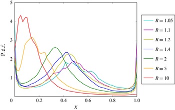
Figure 11. One-dimensional p.d.f.s half-way across the shear layer ( $x/\unicode[STIX]{x1D6FF}=0.5$ ) for various density ratios at times corresponding to $Re_{\unicode[STIX]{x1D6FF}}\approx 8500$ . The p.d.f. for the $R=10$ simulation is displayed at $Re_{\unicode[STIX]{x1D6FF}}\approx 7700$ .

The shear layers entrain more low-density high-speed fluid than high-density low-speed fluid, by volume, at amounts that increase with $R$ (Dimotakis Reference Dimotakis1986). This is consistent with the solution to the self-similar mass conservation equation, shown in figure 3, with asymmetric p.d.f.s (figure 11). This has also been observed in buoyancy-driven flows (Livescu & Ristorcelli Reference Livescu and Ristorcelli2008). Additionally, similarly to spatially developing liquid-phase shear layers, simulated temporally developing gas-phase shear layers also exhibit a constant (in time) and most probable mole fraction (‘non-marching’ hump). This is not commonly reported for gas-phase shear-layer experiments (Meyer, Dutton & Lucht Reference Meyer, Dutton and Lucht2006). Marching versus non-marching p.d.f.s have been reported to depend on initial conditions (Rogers & Moser Reference Rogers and Moser1994; Mattner Reference Mattner2011), in particular, the dimensionality of the initial disturbances, i.e. two- versus three-dimensional (Slessor, Bond & Dimotakis Reference Slessor, Bond and Dimotakis1998). Initial disturbances in this study more closely correspond to the three-dimensional initial perturbations of Slessor et al. (Reference Slessor, Bond and Dimotakis1998), for which they report marching p.d.f.s. For all initial conditions explored (appendix B), non-marching slightly tilted p.d.f. behaviour was ubiquitous in the non-diffusive unsteady growth regimes.

5.2 Spectra

For uniform-density flows at finite Reynolds numbers, spectra are found to scale as $k^{-5/3+q}$ , with $q\rightarrow 0$ with increasing Reynolds numbers (Kolmogorov Reference Kolmogorov1941, Reference Kolmogorov1962; Mydlarski & Warhaft Reference Mydlarski and Warhaft1996). Similar behaviour is observed for variable-density flows at low density ratios (e.g. Batchelor et al. Reference Batchelor, Canuto and Chasnov1992; Livescu & Ristorcelli Reference Livescu and Ristorcelli2008; Chung & Matheou Reference Chung and Matheou2012). However, for variable-density flow, the kinetic energy, as opposed to the specific kinetic energy, is important.

For notational purposes, the spectrum of a field is denoted as $S$ and the spectrum of the fluctuating specific kinetic energy by $S_{\boldsymbol{u}^{\prime }\boldsymbol{\cdot }\boldsymbol{u}^{\prime }}=S_{u^{\prime }u^{\prime }}+S_{v^{\prime }v^{\prime }}+S_{w^{\prime }w^{\prime }}$ , where $\boldsymbol{u}^{\prime }=(u^{\prime },v^{\prime },w^{\prime })$ , omitting the factor of $1/2$ . Spectra shown are spatial one-dimensional spectra along the $z$ direction, at particular $x$ locations, averaged over $y$ . We compare the fields at $x$ values corresponding to $\left\langle \unicode[STIX]{x1D70C}\right\rangle _{y,z}\approx 1$ , where $\left\langle \unicode[STIX]{x1D70C}\right\rangle _{y,z}$ denotes the mean density averaged over $(y,z)$ at $x$ locations where the spectra are calculated.

Spectra shown are also averaged at the corresponding values of $x$ in the two shear layers (cf. figure 1).

In the limit of $R\rightarrow 1$ , the kinetic energy spectrum must yield the specific kinetic energy spectrum, multiplied by the (near-)uniform density. The scaled spectrum, $S_{\boldsymbol{j}^{\prime }\boldsymbol{\cdot }\boldsymbol{j}^{\prime }}/\overline{\unicode[STIX]{x1D70C}}$ , is calculated based on the field $\boldsymbol{j}\equiv \unicode[STIX]{x1D70C}^{1/2}\boldsymbol{u}$ , as proposed by Kida & Orszag (Reference Kida and Orszag1992). The kinetic energy spectrum is then computed conventionally. After division by $\overline{\unicode[STIX]{x1D70C}}$ , results should converge to specific kinetic energy spectra in the limit of $R\rightarrow 1$ .

Figure 12. Spectra for seven density ratios at times corresponding to $Re_{\unicode[STIX]{x1D6FF}}\approx 8500$ . Spectra for $R=10$ are displayed at $Re_{\unicode[STIX]{x1D6FF}}\approx 7700$ . (a) Specific kinetic energy (solid lines) and kinetic energy (dashed lines) spectra, (b) vorticity (solid lines) and specific vorticity (dashed lines) spectra.

To facilitate comparisons and as suggested above, figure 12(a) plots specific kinetic energy spectra (solid lines), $S_{\boldsymbol{u}^{\prime }\boldsymbol{\cdot }\boldsymbol{u}^{\prime }}$ , and kinetic energy spectra divided by $\overline{\unicode[STIX]{x1D70C}}$ (dashed lines), $S_{\boldsymbol{j}^{\prime }\cdot \boldsymbol{j}^{\prime }}/\overline{\unicode[STIX]{x1D70C}}$ , non-dimensionalized by $\unicode[STIX]{x1D716}^{-1/4}\unicode[STIX]{x1D708}^{-5/4}$ . The specific kinetic energy dissipation rate is $\unicode[STIX]{x1D716}$ and $\unicode[STIX]{x1D708}=\unicode[STIX]{x1D707}/\left\langle \unicode[STIX]{x1D70C}\right\rangle _{y,z}$ is a kinematic viscosity, with both averaged over $(y,z)$ -planes at the same $x$ locations.

The panels in figure 12 display spectra at different times, corresponding to similar Reynolds numbers of $Re_{\unicode[STIX]{x1D6FF}}\approx 8500$ for six simulations, with $Re_{\unicode[STIX]{x1D6FF}}\approx 7700$ for the $R=10$ simulation, the largest Reynolds number attained at that density ratio. Spectra are plotted versus wavenumber, $k_{z}$ , scaled with $\unicode[STIX]{x1D702}$ , where $\unicode[STIX]{x1D702}=(\unicode[STIX]{x1D708}^{3}/\unicode[STIX]{x1D716})^{1/4}$ , the plane-averaged Kolmogorov length scale.

Figure 12(a) reveals approximately one decade of power-law scaling. Including density in the autocorrelation through the $\boldsymbol{j}$ dynamic variable has only a small effect on the spectra and does not alter their power-law scaling. The two sets of spectra are similar, as also reported by Kida & Orszag (Reference Kida and Orszag1992) in their investigation of smaller density variations, i.e. $\unicode[STIX]{x1D70C}^{\prime }/\overline{\unicode[STIX]{x1D70C}}\leqslant 0.18$ , in simulations of compressible turbulence. The close match between kinetic energy and specific kinetic energy spectra is not attributable to statistical independence between the density and velocity fields. As evident from the flow geometry, this is not expected.

Figure 12(b) displays non-dimensionalized vorticity spectra, $S_{\unicode[STIX]{x1D74E}^{\prime }\boldsymbol{\cdot }\unicode[STIX]{x1D74E}^{\prime }}$ (solid lines), and non-dimensionalized specific vorticity spectra, $S_{(\unicode[STIX]{x1D74E}/\unicode[STIX]{x1D70C})^{\prime }\cdot (\unicode[STIX]{x1D74E}/\unicode[STIX]{x1D70C})^{\prime }}$ (dashed lines). As with kinetic energy, including density in the vorticity spectra has a small effect, albeit a slightly larger effect than for kinetic energy.

The transport equation for specific vorticity, $\unicode[STIX]{x1D74E}/\unicode[STIX]{x1D70C}$ , in variable-density flow can be written as,

where $\unicode[STIX]{x1D668}=(\unicode[STIX]{x1D735}\boldsymbol{u}+\unicode[STIX]{x1D735}\boldsymbol{u}^{\text{T}})/2$ is the local strain rate tensor and $\unicode[STIX]{x1D749}$ is the viscous stress tensor. In this formulation, no dilatation term appears and density enters through its reciprocal, motivating the investigation of specific vorticity in figure 12(b).

Figure 13. One-dimensional compensated spectra in $z$ for flow with $R=1.4$ at various Reynolds numbers. Note the different $x$ axis, which is scaled by the (outer-scale) shear-layer width, $\unicode[STIX]{x1D6FF}(t)$ , as opposed to the inner-scale of $\unicode[STIX]{x1D702}$ in figure 12. Spectra are multiplied by $(k_{z}\ell )^{5/3-q}$ , where $\ell =L/2$ half the computational domain width, and $q=0.3$ . The black horizontal line is for reference.

To explore the spectral dependence on Reynolds number, figure 13 displays one-dimensional kinetic energy spectra for $R=1.4$ . These are compensated (multiplied by $(k_{z}\ell )^{5/3-q}$ , with $q=0.3$ ) and exhibit very small slopes over about a decade, with slopes slightly decreasing with increasing Reynolds number, terminating with the viscous attenuation at small scales, i.e. progressively higher wavenumbers. The value $q=0.3$ was determined by fitting slopes to achieve nearly horizontal lines for the larger Reynolds numbers and is consistent with findings by Mydlarski & Warhaft (Reference Mydlarski and Warhaft1996). Figure 13 demonstrates the larger-scale wavenumber separation with increasing Reynolds number, as expected.