


1. Introduction
Modal analysis is a well-known method to study systems of partial differential equations (PDEs). By studying characteristics of a dynamic system, one can compute a basis in the PDE solution space and, thus, identify the underlying coherent structures governing the system's evolution in time and space. For instance, it is a established technique to develop reduced-order models (ROMs) of complex flows (Rowley & Dawnson Reference Rowley and Dawnson2017; Taira et al. Reference Taira, Hemati, Brunton, Sun, Duraisamy, Bagheri, Dawson and Yeh2020).
In the context of dynamical systems, a popular method is proper orthogonal decomposition (POD), also called principal component analysis or Karhunen–Loève decomposition in other disciplines. Introduced to the fluid dynamics community by Lumley (Reference Lumley1967, Reference Lumley1970), the statistical method decomposes an ensemble of bounded signals into orthogonal deterministic modes (often called empirical eigenfunctions) which, within all possible linear decompositions, are optimal in containing the most energy in an average sense (Berkooz, Holmes & Lumley Reference Berkooz, Holmes and Lumley1993).
The POD method enables the decomposition of velocity correlations from statistically stationary flows into modes, in order to identify and analyse the most energetic structures evolving in space and time. Due to its generality and solid foundation in the statistics theory, POD has been applied to numerous fluid dynamics fields, with studies involving coherent structures in turbulence (Sirovich Reference Sirovich1987), derivations of ROMs (Ravindran Reference Ravindran2000; Noack et al. Reference Noack, Afanasiev, Morzyński, Tadmor and Thiele2003), among many other applications. The method gained special traction in the 1990s with the rapid development of numerical analysis and computational tools (Aubry Reference Aubry1991).
For statistically stationary flows, the application of POD over the Fourier transform in time of measured correlations generates modes that develop in a single frequency and display coherence in both space and time. This approach has been applied throughout the years to study jets (Glauser & George Reference Glauser and George1987; Delville et al. Reference Delville, Ukeiley, Cordier, Bonnet and Glauser1999; Picard & Delville Reference Picard and Delville2000; Jung, Gamard & George Reference Jung, Gamard and George2004; Iqbal & Thomas Reference Iqbal and Thomas2007; Tinney & Jordan Reference Tinney and Jordan2008; Gudmundsson & Colonius Reference Gudmundsson and Colonius2011; Schmidt et al. Reference Schmidt, Towne, Colonius, Cavalieri, Jordan and Brès2017), mixing layers (Arndt, Long & Glauser Reference Arndt, Long and Glauser1997; Bonnet et al. Reference Bonnet1998; Citriniti & George Reference Citriniti and George2000), turbulent pipes (Hellström & Smits Reference Hellström and Smits2014), boundary layers (Tutkun & George Reference Tutkun and George2017) and wakes (Araya, Colonius & Dabiri Reference Araya, Colonius and Dabiri2017).
This form of POD in the frequency domain has been labelled spectral POD, or SPOD (Towne, Schmidt & Colonius Reference Towne, Schmidt and Colonius2018; Schmidt & Colonius Reference Schmidt and Colonius2020). It should be noted that we do not refer here to the homonym work of Sieber, Paschereit & Oberleithner (Reference Sieber, Paschereit and Oberleithner2016), which deals with a different algorithm. Towne et al. (Reference Towne, Schmidt and Colonius2018) established an important link between statistics and dynamical systems in the frequency space, as a linear set of equations, forced with an uncorrelated (spatially white) noise in a given frequency must have SPOD modes identical to the modes obtained via resolvent analysis. This property is not always present in the form of POD, which yields purely spatial modes modulated by time-dependent coefficients, hereby called spatial POD.
Later works employing SPOD include: the development of data-driven ROMs for boundary layer transition control (Sasaki et al. Reference Sasaki, Morra, Cavalieri, Hanifi and Henningson2020), characterisation of noise generated over airfoils (Sano et al. Reference Sano, Abreu, Cavalieri and Wolf2019; Abreu et al. Reference Abreu, Tanarro, Cavalieri, Schlatter, Vinuesa, Hanifi and Henningson2021) and the identification of coherent structures in channels (Abreu et al. Reference Abreu, Cavalieri, Schlatter, Vinuesa and Henningson2020a), wakes (Nidhan et al. Reference Nidhan, Chongsiripinyo, Schmidt and Sarkar2020; Li et al. Reference Li, Chen, Liang, Liu and Xiong2021), separated high-speed flows (Lugrin et al. Reference Lugrin, Beneddine, Leclercq, Garnier and Bur2021) and complex geometries (Zhang, Ooka & Kikumoto Reference Zhang, Ooka and Kikumoto2021; He et al. Reference He, Fang, Rigas and Vahdati2021).
Despite its versatility, the proposed SPOD algorithm (Towne et al. Reference Towne, Schmidt and Colonius2018) leads to some inherent complexity related to spectral estimation. It relies on the Welch method (Welch Reference Welch1967) for the estimation of the cross-spectral density (CSD) tensor, and hence, computed gains and modes are sensitive to sampling parameters (number of field snapshots/realisations  $N_t$, time step
  $\delta t$) and estimation parameters (number of blocks,
  $N_b$, number of snapshots per block,
  $N_{FFT}$, windowing function,
  $w(t)$, and overlap between successive blocks,
  $O_{FFT}$). For a given dataset with
  $N_t$ snapshots separated by a constant time step
  $\delta t$, increasing
  $N_b$ implies decreasing
  $N_{FFT}$ and vice versa. A larger
  $N_b$ penalises frequency resolution, increases spectral leakage and may lead to results contaminated with statistical bias, whereas a larger
  $N_{FFT}$ penalises convergence by decreasing the number of averaging blocks. The appropriate compromise between these cases is problem dependent and literature concerning which choice yields the best convergence for a given dataset is lacking, even though statistical confidence bounds can be derived for computed SPOD gains (Schmidt & Colonius Reference Schmidt and Colonius2020). In general, estimation parameters are chosen subjectively based on the researcher's experience and convergence is checked a posteriori.
Moreover, mode convergence can be slow and difficult to verify as the method requires long time-resolved datasets. For Navier–Stokes simulations, this translates to high computational and storage costs that are often impracticable. A proposed alternative to reduce overall requirements of memory is the streaming SPOD algorithm proposed by Schmidt & Towne (Reference Schmidt and Towne2019). By accessing only one temporal snapshot at a time and incrementing the SPOD at each step, the algorithm allows for the use of arbitrarily long time series and real-time processing, avoiding storage costs, but maintaining long computations that may be expensive.
This work discusses the effects of estimation parameters on the convergence of the SPOD method. We first examine a model Ginzburg–Landau system which mimics the dynamics of turbulent jets. In sequence, the results from this convergence analysis are used to propose a new method based on a temporal shift to further reduce SPOD errors and enable a more accurate analysis of simulations with shorter integration times. In order to demonstrate its applicability to fluid flows, the shifting algorithm is applied to a boundary layer over a flat plate subject to bypass transition.
For flat-plate boundary layers, modal transition by Tollmien–Schlichting waves is bypassed for free-stream turbulence levels greater than around 1 % (Matsubara & Alfredsson Reference Matsubara and Alfredsson2001) as the transition occurs from the linear growth of streamwise elongated, low-frequency structures, with alternating high and low velocity, called streaks. The work of Ellingsen & Palm (Reference Ellingsen and Palm1975) shows that perturbations in flows with low variation along the streamwise direction can be algebraically amplified through the transient growth caused by the interaction of non-normal Orr–Sommerfeld modes, even in cases where modal stability predicts an exponential decay. This phenomenon is known in the literature as the lift-up effect (Brandt Reference Brandt2014). In bypass conditions, the streaks caused by the lift-up effect might be amplified enough to trigger nonlinear interactions and degenerate to turbulence in Reynolds numbers below the critical levels provided by the linear theory of exponential growth (Brandt, Schlatter & Henningson Reference Brandt, Schlatter and Henningson2004).
Streaks appear as SPOD modes with vanishing frequency (Sasaki et al. Reference Sasaki, Morra, Cavalieri, Hanifi and Henningson2020), and numerical convergence in such cases is challenging (Pickering et al. Reference Pickering, Rigas, Nogueira, Cavalieri, Schmidt and Colonius2020). Hence, detection of coherent structures in a database of bypass transition of a boundary layer is a relevant test of convergence of SPOD modes and of the potential improvements that may be obtained with the proposed temporal shift of the database.
The remainder of the manuscript is organised as follows. Sections 2 and 3 review methods used in SPOD and resolvent analysis. In § 4 the temporal shift is introduced and its effects are discussed, with guidance on how to choose shifting parameters. Finally, in § 5 the results of the application of these concepts in the Ginzburg–Landau system and the flat-plate case are evaluated.
2. Spectral POD
Spectral POD is a modal analysis method aimed at extracting the most energetic turbulent coherent structures which evolve in a single frequency from statistically stationary data. A brief explanation of the algorithm is developed in this section. The computation involves the snapshot method, and further information can be found in Towne et al. (Reference Towne, Schmidt and Colonius2018) and Schmidt & Colonius (Reference Schmidt and Colonius2020).
Considering a turbulent flow dataset with  $M$ degrees of freedom (number of variables times number of spatial points
  $N_x$) and
  $N_t$ snapshots taken at a fixed interval
  $\delta t$ (each one treated as an independent realisation based on the ergodicity argument), we define the state vector
  $\boldsymbol {q} \in \mathbb {C}^{M}$ with a chosen inner product as
 \begin{equation} \left\langle \boldsymbol{q}_{1}, \boldsymbol{q}_{2}\right\rangle_{\boldsymbol{W}}=\boldsymbol{q}_{1}^{H} \boldsymbol{\mathsf{W}} \boldsymbol{q}_{2}, \end{equation}
where  $\boldsymbol{\mathsf{W}}^{M \times M}$ is a square positive definite diagonal matrix, and
  $\{\,\cdot\,\}^H$ is the conjugate transpose. The ensemble of realisation vectors are then used to construct the data matrix
 \begin{equation} \boldsymbol{\mathsf{Q}}=\left[\begin{array}{cccccc} \mid & \mid & & \mid \\ \boldsymbol{q}_{1} & \boldsymbol{q}_{2} & \cdots & \boldsymbol{q}_{N_t} \\ \mid & \mid & & \mid \end{array}\right], \quad \boldsymbol{\mathsf{Q}} \in \mathbb{C}^{M \times N_t}. \end{equation}
 For the case of an incompressible flow, each component of the velocity field  $\boldsymbol {u}(\boldsymbol {x},t)=(u(\boldsymbol {x},t),v(\boldsymbol {x},t),w(\boldsymbol {x},t))$ is a variable. In that case, we can construct the vector
  $\boldsymbol {q} \in \mathbb {C}^{3 N_x}$ by computing the zero-mean velocity fluctuations for each snapshot, i.e.
 \begin{equation} \boldsymbol{\tilde{u}}(\boldsymbol{x},t) = \boldsymbol{u}(\boldsymbol{x},t) - \boldsymbol{\mathsf{U}}(\boldsymbol{x}) = (\tilde{u}(\boldsymbol{x},t),\tilde{v}(\boldsymbol{x},t),\tilde{w} (\boldsymbol{x},t)), \end{equation}
with  $\boldsymbol{\mathsf{U}}(\boldsymbol {x})$ being the mean field, and subsequently mapping all fluctuation components to a column vector in a convenient order, for example,
 \begin{equation} \boldsymbol{q}_i \!=\! \left[\begin{array}{ccccccccc} \tilde{u}(\boldsymbol{x_1},i) & \cdots & \tilde{u}(\boldsymbol{x}_{N_x},i) & \tilde{v}(\boldsymbol{x_1},i) & \cdots & \tilde{v}(\boldsymbol{x}_{N_x},i) & \tilde{w}(\boldsymbol{x_1},i) & \cdots & \tilde{w}(\boldsymbol{x}_{N_x},i) \end{array}\right]^{\rm T}. \end{equation}
2.1. Spectral estimation
For the estimation of the CSD matrix  $\boldsymbol{\mathsf{C}}$, the Welch method is employed. The data matrix
  $\boldsymbol{\mathsf{Q}}$ is decomposed into
  $N_b$ successive blocks containing
  $N_{FFT}$ realisations, with
  $O_{FFT}$ overlapped realisations between consecutive blocks. Then, the discrete Fourier transform (DFT) in time, weighted by a windowing function
  $w(t)$, is computed for each block.
Given  $\boldsymbol {\hat {q}}_k(\omega )$, the vector resulting from the DFT at a frequency
  $\omega$ for the
  $k$th block, we can assemble the vectors from all blocks corresponding to this frequency in a spectral data matrix
 \begin{equation} \hat{\boldsymbol{\mathsf{Q}}}_\omega=\left[\begin{array}{cccccc} \mid & \mid & & \mid \\ \boldsymbol{\hat{q}}_{1} & \boldsymbol{\hat{q}}_{2} & \cdots & \boldsymbol{\hat{q}}_{N_b} \\ \mid & \mid & & \mid \end{array}\right], \quad \hat{\boldsymbol{\mathsf{Q}}}_\omega \in \mathbb{C}^{M \times N_b}, \end{equation}
allowing the CSD matrix for each frequency to be computed as
 \begin{equation} \boldsymbol{\mathsf{C}}_\omega = \frac{1}{N_b} \hat{\boldsymbol{\mathsf{Q}}}_\omega \hat{\boldsymbol{\mathsf{Q}}}_\omega^{H} \boldsymbol{\mathsf{W}}, \quad \boldsymbol{\mathsf{C}}_\omega \in \mathbb{C}^{M \times M} \end{equation}
and finally SPOD gains  $\skew3\hat{\boldsymbol{\varLambda} }$ and modes
  $\skew4\hat{\boldsymbol{\varPsi} }$ are calculated by solving the following eigenproblem of size
  $M \times M$:
 \begin{equation} \boldsymbol{\mathsf{C}}_\omega \skew4\hat{\boldsymbol{\varPsi}}=\skew4\hat{\boldsymbol{\varPsi}} \skew3\hat{\boldsymbol{\varLambda}}. \end{equation}
2.2. Snapshot SPOD
In fluid dynamics applications datasets often have  $M \gg N_b$, as the problems are typically high dimensional and the cost of their simulation typically limits the amount of snapshots that can be obtained and handled. Therefore, it is computationally cheaper to obtain the same modes and gains by solving the much smaller eigenproblem of size
  $N_b \times N_b$ in the row space of the matrix
  $\hat{\boldsymbol{\mathsf{Q}}}_\omega$, as presented by Sirovich (Reference Sirovich1987) and revisited in Towne et al. (Reference Towne, Schmidt and Colonius2018),
 \begin{gather} \boldsymbol{\mathsf{M}}_\omega = \frac{1}{N_b} \hat{\boldsymbol{\mathsf{Q}}}_\omega^{H} \boldsymbol{\mathsf{W}} \hat{\boldsymbol{\mathsf{Q}}}_\omega, \quad \boldsymbol{\mathsf{M}}_\omega \in \mathbb{C}^{N_b \times N_b}, \end{gather}
 \begin{gather} \boldsymbol{\mathsf{M}}_\omega \skew3\hat{\boldsymbol{\varTheta}} = \skew3\hat{\boldsymbol{\varTheta}} \skew3\hat{\boldsymbol{\varLambda}}, \end{gather}
 \begin{gather} \skew4\hat{\boldsymbol{\varPsi}} = \frac{1}{\sqrt{N_b}} \hat{\boldsymbol{\mathsf{Q}}}_\omega \skew3\hat{\boldsymbol{\varTheta}} \skew3\hat{\boldsymbol{\varLambda}}^{{-}1/2}. \end{gather}
3. Resolvent analysis
When applying the Reynolds decomposition to the Navier–Stokes equation, linear and nonlinear terms can be isolated. Then, nonlinear terms may be treated as an input forcing signal to a linear system. In other words, we construct a state-space formulation with input/forcing terms  $\boldsymbol {f}$ related to response/fluctuations terms
  $\boldsymbol {q}$ by a linear operator
  $\boldsymbol{\mathsf{L}}$ that is only a function of time invariant parameters, considering a linearisation of the Navier–Stokes system around a laminar solution (Jovanović & Bamieh Reference Jovanović and Bamieh2005) or a mean flow (McKeon & Sharma Reference McKeon and Sharma2010). Operators
  $\boldsymbol{\mathsf{H}}$ and
  $\boldsymbol{\mathsf{B}}$ are used to restrict spatially the forcing and response, respectively, when necessary. We thus have
 \begin{equation} \left. \begin{aligned} \frac{\partial \boldsymbol{q}}{\partial t} & = \boldsymbol{\mathsf{L}} \boldsymbol{q} + \boldsymbol{\mathsf{B}}\boldsymbol{f}, \\ \boldsymbol{y} & = \boldsymbol{\mathsf{H}} \boldsymbol{q}, \end{aligned} \right\} \end{equation}
and by taking the Fourier transform in time we obtain
 \begin{gather} \left. \begin{aligned} \left({\rm i} \omega \boldsymbol{\mathsf{I}} - \boldsymbol{\mathsf{L}}\right) \boldsymbol{\hat{q}} & = \boldsymbol{\mathsf{B}}\boldsymbol{\hat{f}},\\ \boldsymbol{\hat{y}} & = \boldsymbol{\mathsf{H}} \boldsymbol{\hat{q}}, \end{aligned} \right\} \end{gather}
 \begin{gather} \boldsymbol{\hat{y}} = \boldsymbol{\mathsf{R}} \boldsymbol{\hat{f}} \implies \boldsymbol{\mathsf{R}} = \boldsymbol{\mathsf{H}}\left({\rm i} \omega \boldsymbol{\mathsf{I}} - \boldsymbol{\mathsf{L}}\right)^{{-}1}\boldsymbol{\mathsf{B}}, \end{gather}
where  $\boldsymbol{\mathsf{R}}$ is called the resolvent operator. Now, resolvent response modes
  $\boldsymbol{\mathsf{U}}$, forcing modes
  $\boldsymbol{\mathsf{V}}$ and gains
  $\boldsymbol{\varSigma}$ (ratio between the norms of
  $\boldsymbol {y}$ and
  $\boldsymbol {f}$) can be computed via the singular value decomposition (SVD)
 \begin{equation} \tilde{\boldsymbol{\mathsf{R}}} \tilde{\boldsymbol{\mathsf{V}}} = \tilde{\boldsymbol{\mathsf{U}}} \boldsymbol{\varSigma}. \end{equation}
 From the resolvent framework (3.3), the response CSD matrix  $\boldsymbol{\mathsf{C}}_\omega$ can be computed directly as a function of the forcing CSD matrix
  $\boldsymbol{\mathsf{F}}_\omega$. Assuming that
 \begin{equation} \boldsymbol{\mathsf{C}}_\omega = \mathcal{E}\left(\boldsymbol{\hat{y}} \boldsymbol{\hat{y}}^H\right), \quad \boldsymbol{\mathsf{F}}_\omega = \mathcal{E}\left(\boldsymbol{\hat{f}} \boldsymbol{\hat{f}}^H\right), \end{equation}
where  $\mathcal {E}(\,\cdot \,)$ stands for the average over all realisations, we have
 \begin{equation} \boldsymbol{\mathsf{C}}_\omega = \boldsymbol{\mathsf{R}} \boldsymbol{\mathsf{F}}_\omega \boldsymbol{\mathsf{R}}^H. \end{equation}
 If forcing terms are perfectly uncorrelated,  $\boldsymbol{\mathsf{F}}_\omega = \boldsymbol{\mathsf{I}}$, the expression can be reduced to
 \begin{equation} \boldsymbol{\mathsf{C}}_\omega = \boldsymbol{\mathsf{R}} \boldsymbol{\mathsf{R}}^H \end{equation}
and, from (3.4), we have
 \begin{equation} \boldsymbol{\mathsf{C}}_\omega = \boldsymbol{\mathsf{U}} \boldsymbol{\varSigma}^2 \boldsymbol{\mathsf{U}}^{{-}1} \implies \boldsymbol{\mathsf{C}}_\omega \boldsymbol{\mathsf{U}} = \boldsymbol{\mathsf{U}} \boldsymbol{\varSigma}^2 \end{equation}
leading to
 \begin{equation} \skew4\hat{\boldsymbol{\varPsi}} = \boldsymbol{\mathsf{U}}, \quad \skew3\hat{\boldsymbol{\varLambda}} = \boldsymbol{\varSigma}^2 \end{equation}
from (2.7).
This shows that resolvent response modes are equal to those obtained via the SPOD method for a system forced with spatially white forcing (Towne et al. Reference Towne, Schmidt and Colonius2018), a property also true for an arbitrary inner-product norm (see Appendix A).
In this study the mode equivalence property is exploited to study numerically the convergence of SPOD modes by employing a simple linear system analogous to the Navier–Stokes system, forced with spatially uncorrelated signals, and comparing resolvent and SPOD results.
4. Temporal shift
The idea of introducing a temporal shift to compensate for transport in signal processing and modal decomposition is not new. The work of Reiss et al. (Reference Reiss, Schulze, Sesterhenn and Mehrmann2018), for instance, discusses its application on the construction of ROMs and proposes a shifted method based on spatial POD to address the slow decay of energy observed from the modal decomposition of transport dominated phenomena. However, to the best of our knowledge, the application of a time delay in SPOD has not been attempted.
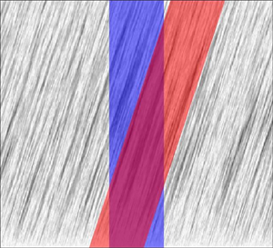
The Welch method employed in the SPOD method separates the dataset in blocks of a chosen time length. For transport dominated phenomena with elongated domains, one can usually choose signals corresponding to coordinates  $\boldsymbol {x_1}$ and
  $\boldsymbol {x_2}$ where the time lag for peak cross-correlation is greater than the block time length. The effect is shown in figure 1 with the blue rectangle, which illustrates the standard situation where the same initial and final times of Welch blocks are taken for all positions in the flow. This causes an apparent loss of coherence and encumbers the statistical convergence of the decomposition. This feature was observed, for instance, by Jaunet, Jordan & Cavalieri (Reference Jaunet, Jordan and Cavalieri2017).

Figure 1. Diagram illustrating the effect of the temporal shift on the model system presented in § 5.1. In standard conditions, the cross-correlation peak lies outside the chosen time window. The application of the expected time lag between signals in positions  $x_1$ and
  $x_2$ maintains the peak inside the same time window. The operator
  $\langle \,\cdot \,\rangle$ denotes the expected value.
4.1. Proposed algorithm
In order to address the limitations imposed by the Welch method, we propose an extension to the SPOD algorithm in two steps, exploiting the assumed stationarity: we first apply a shift in time and then correct the phase in Fourier space, in a procedure that preserves asymptotic convergence to the true CSD (see Appendix B). The temporal shift aims at improving convergence for a window of finite size by maximising cross-correlations within each Welch block, via the insertion of an expected time delay to each spatial location.
Concerning the SPOD implementation, first we treat the data matrix  $\boldsymbol{\mathsf{Q}}$ by means of a data shift and then correct the effects of this treatment after the application of the Welch method. Given a point of interest with streamwise coordinate
  $x_p$ and a matrix
  $\boldsymbol{\mathsf{Q}}$ with
  $N_x$ rows and
  $N_t$ columns, for each row
  $k$, the columns are shifted by
 \begin{equation} s_k = \frac{\Delta x}{U_k \delta t}, \quad \Delta x = x_p-x_k \end{equation}
positions. In this expression  $x_k$ is the point's streamwise coordinate,
  $\delta t$ is the time step between realisations and
  $U_k$ is a chosen velocity so that
  $\Delta x /U_k$ approximates the time lag for peak cross-correlation with respect to the point of interest. For instance, the dominant convection velocity could be used, if this information is readily available. Moreover, there is no requirement for
  $U_k$ to be constant throughout the domain.
Columns at the beginning or the end of the time series, for which the time shift  $s_k$ is not possible, are removed from the computation. This can be more easily implemented as a circular shift of the data removing the columns for which there is an artificial overlap between the end of the time series at one point and the beginning of the series at another point.
It is important to note that, if  $s_k$ is not an integer, the shift must be interpolated, as discussed in Reiss et al. (Reference Reiss, Schulze, Sesterhenn and Mehrmann2018). Given
  $\mathcal {Z}^s_k$, the operator that circularly shifts a line
  $k$ by
  $s$ positions, and
  $\tilde {\boldsymbol{\mathsf{Q}}}$ the resulting shifted matrix, the linearly interpolated shifting operation takes the form
 \begin{equation}
\tilde{\boldsymbol{\mathsf{Q}}} = \left\{ \begin{array}{@{}ll} \mathcal{Z}^{s_k}_k
\boldsymbol{\mathsf{Q}} & \text{if} \ s_k \in
\mathbb{Z}, \\ \left(\lceil s_k \rceil -
s_k\right) \cdot \mathcal{Z}^{\lfloor s_k \rfloor}_k
\boldsymbol{\mathsf{Q}} + \left(s_k - \lfloor s_k \rfloor\right)
\cdot \mathcal{Z}^{\lceil s_k \rceil}_k \boldsymbol{\mathsf{Q}}
& \text{otherwise}. \end{array}\right.
\end{equation}
\begin{equation}
\tilde{\boldsymbol{\mathsf{Q}}} = \left\{ \begin{array}{@{}ll} \mathcal{Z}^{s_k}_k
\boldsymbol{\mathsf{Q}} & \text{if} \ s_k \in
\mathbb{Z}, \\ \left(\lceil s_k \rceil -
s_k\right) \cdot \mathcal{Z}^{\lfloor s_k \rfloor}_k
\boldsymbol{\mathsf{Q}} + \left(s_k - \lfloor s_k \rfloor\right)
\cdot \mathcal{Z}^{\lceil s_k \rceil}_k \boldsymbol{\mathsf{Q}}
& \text{otherwise}. \end{array}\right.
\end{equation}
After application of the Welch method the  $k$th row of each resulting
  $\hat {\boldsymbol{\mathsf{Q}}}_\omega$ matrix, with
  $N_x$ rows and
  $N_b$ columns, is multiplied by
  $\exp (-\textrm {i} \omega s_k \delta t)$ to correct the phase created by the previous temporal shift operation, according to the properties of the Fourier transform.
This procedure will be referred to in this work as a shifted SPOD, for the sake of concision, and should not be considered a new variety of POD, but instead a new algorithm for the method we call SPOD.
Computationally, the shifting algorithm deals with row-wise rearrangements of matrix elements and also row-wise array multiplications, which are low complexity operations when compared with Fourier transforms and eigenproblems. Once the data matrices are loaded in memory, both these steps should be rapidly performed on a modern desktop computer without the addition of expressive cost to the SPOD method.
4.2. On the choice of point of interest, shifting velocity and window size
The choice of window size  $N_{FFT}$ and, consequently, the number of blocks
  $N_b$ is the most subjective step of the SPOD method. For a given database, it is not obvious how one should choose the most appropriate number of realisations per block that simultaneously ensures blocks are long enough in time to properly capture the evolution of the most energetic structures and numerous enough to reduce the decomposition's variance.
Here, we discuss this choice and propose a pre-processing analysis to objectively set a suitable  $N_{FFT}$ for a given dataset, considering a shifting velocity and point of interest. This procedure is also applicable to the standard SPOD, as it can be treated as a special case of the shifted SPOD with shifting velocity
  $U_k \to \infty$. The procedure follows four steps.
(i) Given a preferential flow direction
 $X$, we choose a point of interest $p$ of coordinate $x_p$ contained in the region from which we want to extract the most energetic structures. For simulations, it is important to avoid points under the influence of numerical boundaries, such as inlets, outlets and sponge/fringe zones, in order to guarantee that computed two-point correlations are physical.
(ii) Once
$p$ is chosen, we compute the space–time correlations at positions along the $X$ direction with respect to the signal at $x_p$, as later illustrated in figure 4(a). In the case of multi-dimensional data, cross-correlations can be computed at multiple slices, as will be later shown in figure 14(a,c,e), or for multiple vector components.(iii) The inclination of the peak correlations quantifies the dominant convection velocity, which might vary as a function of position and not necessarily match the local mean velocity (He, Jin & Yang Reference He, Jin and Yang2017). By applying a shifting velocity that approximates said dominant velocity, it is possible to align correlation peaks, as later discussed in figures 4(b) and 14(b,d, f), in order to generate a vertical band of high correlation in time. This narrower correlation allows a given window to capture more kinematic information about the system. However, if a dominant velocity cannot be identified, the shifting operation should yield no special benefit.
(iv) From the space–time plot we are finally able to determine the smallest window size capable of capturing the bulk of correlation, which simultaneously resolves the frequencies of interest in the study. By narrowing the correlation band in time, the shifting algorithm admits even smaller window sizes for the same amount of correlation captured and, thus, reduces overall variance by increasing the number of blocks
$N_b$. In this way, it becomes feasible to objectively set the $N_{FFT}$ parameter based on the individual characteristics of each database and frequency resolution requirements.


5. Convergence analysis of SPOD
5.1. A model problem: Ginzburg–Landau equation
The complex-valued Ginzburg–Landau equation (CGLE) has been one of the most studied equations in a wide variety of physics fields to provide insight over the dynamics of non-equilibrium phenomena in spatially extended systems (Aranson & Kramer Reference Aranson and Kramer2002). Particularly in the field of fluid dynamics and turbulence, the one-dimensional linearised complex Ginzburg–Landau equation is often employed to model instabilities in spatially evolving flows for its properties of advection and diffusion (Huerre & Monkewitz Reference Huerre and Monkewitz1990; Bagheri et al. Reference Bagheri, Henningson, Hœpffner and Schmid2009; Cavalieri, Jordan & Lesshafft Reference Cavalieri, Jordan and Lesshafft2019). The equation is written in the input–output framework as
 \begin{equation} \frac{\partial \boldsymbol{q}}{\partial t} + U \frac{\partial \boldsymbol{q}}{\partial x} - \mu(x)\boldsymbol{q} - \gamma \frac{\partial^2 \boldsymbol{q}}{\partial x^2} = \boldsymbol{f}, \end{equation}
with  $\boldsymbol {q}$ and
  $\boldsymbol {f}$ being output response and input forcing, respectively, and rewritten in Fourier space as
 \begin{equation} \left({\rm i} \omega \boldsymbol{\mathsf{I}} + U \frac{\partial}{\partial x} - \mu(x) - \gamma \frac{\partial^2}{\partial x^2}\right) \boldsymbol{\hat{q}} = \boldsymbol{\hat{f}} \end{equation}
from which the resolvent operator can be computed as
 \begin{equation} \boldsymbol{\mathsf{R}} = \left({\rm i} \omega \boldsymbol{\mathsf{I}} + U \frac{\partial}{\partial x} - \mu(x) - \gamma \frac{\partial^2}{\partial x^2}\right)^{{-}1} \end{equation}
with an inverse obtained after a discretisation of the derivatives to form the operators in matrix form.
When the system is forced with spatially white statistics on a given frequency  $\omega$, the SPOD modes
  $\boldsymbol {\hat {\psi }}(\omega )$ are identical to the resolvent response modes,
  $\boldsymbol {u}(\omega )$. Thus, such response modes, which are deterministic in nature, are used to quantify the SPOD convergence defined in terms of the error
 \begin{equation} \varepsilon(\omega) = 1 - \frac{| \langle \boldsymbol{\hat{\psi}}(\omega),\boldsymbol{u}(\omega) \rangle|}{\|\boldsymbol{\hat{\psi}}(\omega)\| \,\cdot\, \|\boldsymbol{u}(\omega)\|}, \end{equation}
where the operators  $\langle\,\cdot ,\cdot\,\rangle$ and
  $\|\,\cdot \,\|$ are respectively the Euclidean inner product and norm.
The model problem was devised according to Cavalieri et al. (Reference Cavalieri, Jordan and Lesshafft2019) and parameters
 \begin{gather} \mu (x) = A\left(1-\frac{x}{10}\right), \end{gather}
 \begin{gather} \gamma = \frac{1-{\rm i}}{10}, \end{gather}
were set to mimic the dynamics of turbulent jets. Three distinct cases were investigated: case 1 with  $U=10$ and
  $A=0.6$; case 2 with
  $U=12$ and
  $A=1$; case 3 with
  $U=14$ and
  $A=1.25$. These choices lead to a varying convection velocity between the three cases, which modifies the correlation peaks discussed in § 4. Numerical solutions were obtained using a Crank–Nicolson scheme for time marching. Spatial discretisation was set using a fixed grid spacing of
  $\Delta x = 0.1$, with a total of
  $N_x = 300$ points,
  $x \in [0,30]$ and
  $q(0)=q(30)=0$. A second-order upwind scheme was applied for the first spatial derivative and a second-order centred scheme for the second. Because of the uniform grid, the inner-product matrix
  $\boldsymbol{\mathsf{W}}$ is set as
  $I\Delta x$ to account for the spatial quadrature.
The forcing is applied by adding a random complex number with a uniformly distributed phase and amplitude to the value at each grid point for every time step. To ensure that fluctuations are adequately resolved in frequency, we apply to the forcing signal a finite impulse response low-pass filter of 30th order in time, with cutoff at 60 % of the Nyquist frequency. Numerical integration is done for a range of 500 time units using a time step of  $\delta t = 0.01$, generating a total of
  $N_t = 5\times 10^4$ snapshots per case.
5.1.1. Computation of SPOD modes
In order to understand how SPOD errors scale as a function of sampling and estimation parameters for each model case, the number of snapshots  $N_{FFT}$ within each block is varied from 100 to 5000 in steps of 100 and the number of blocks
  $N_b$ set accordingly to comprise all
  $N_t$ snapshots (fixed-data analysis). This configuration ensures that all computations reach exactly the frequency
  $\omega =2{\rm \pi}$, which has the same order of magnitude of the most energetic frequency in all three cases, in order to compare SPOD and resolvent modes.
To reduce spectral leakage effects and allow for the use of a relatively large consecutive block overlapping of  $O_{FFT} = \lfloor 0.75 \: N_{FFT} \rfloor$, we apply to each block an infinitely smooth windowing function of the form
 \begin{equation} w_{C^{\infty}_2}(t)= \left\{\begin{array}{ll} \mathrm{e}^{8} / \mathrm{e}^{{2 T^{2}}/(t(T-t))}, & 0< t< T, \\ 0 & \text{otherwise, } \end{array}\right. \end{equation}
with all derivatives equal to zero at  $0$ and
  $T$ (Martini et al. Reference Martini, Cavalieri, Jordan and Lesshafft2020).
The error between SPOD and resolvent modes, defined in (5.4), is shown in figure 2 for the leading four SPOD modes at frequency  $\omega =2 {\rm \pi}$. The results obtained indicate that better absolute convergence is related to window length, normalised by domain size, and convection velocity. Thus, we define a normalised window size
 \begin{equation} N_{norm} = \frac{N_{FFT} \delta t}{T_c} , \quad T_c = \frac{L}{U}, \end{equation}
where  $T_c$ is the time taken to cross the entire domain based on the parameter
  $U$ of the CGLE system and
  $L$ is the total length of the domain.

Figure 2. Spectral POD estimation error  $\varepsilon$ at frequency
  $\omega =2 {\rm \pi}$, plotted against the normalised window length
  $N_{norm}$. Legend: (
 $\circ$, blue) case 1; (
 $\times$, red) case 2; (
 $*$, orange) case 3. (a) Mode 1; (b) mode 2; (c) mode 3; (d) mode 4.
The graphs in figure 2 show that SPOD modes computed with very low values of  $N_{norm}$ yield the worst convergence. In that scenario, the Welch blocks are too short to correctly capture the evolution of coherent structures in time, which leads to statistically biased results. On the other side, for larger
  $N_{norm}$ values, errors tend to stabilise or even increase for higher modes (modes 3 and 4) due to the reduced number of averaging blocks and consequent increase in noise.
A trade-off between estimation bias, which is reduced with increasing window sizes, and estimation variance, i.e. statistical noise, which increases with window size (lower number of samples), is thus required. Effects of bias and noise are illustrated in figure 3.

Figure 3. Mode 1 at frequency  $\omega =2 {\rm \pi}$ for case 3. Other cases display similar features. (a) Resolvent operator response mode; (b) SPOD mode with
  $N_{FFT}=100$,
  $N_b=1997$ and
  $N_{norm} \approx 0.5$: higher precision, lower accuracy (bias); (b) SPOD mode with
  $N_{FFT}=600$,
  $N_b=330$ and
  $N_{norm} \approx 3$; (c) SPOD mode with
  $N_{FFT}=5000$,
  $N_b=37$ and
  $N_{norm} \approx 23$: lower precision, higher accuracy (noise). Legend: (orange) absolute value; (blue) real part; (red) imaginary part; (dotted lines) resolvent mode for comparison.

Figure 4. Space–time cross-correlation with respect to the point  $x_p=15$ for case 2 (
 $U=12$,
  $A=1$). Other cases display similar features. (a) No shift; (b) optimal shift.
Overall, a normalised window size between 2 and 4 is a good compromise to achieve the best convergence across the first four SPOD modes in these cases. This implies that a time series should be sufficiently long to comprise a large number of blocks of normalised window size between 2 and 4. This would translate to a database with several flow-through times, which may be quite expensive to compute and store if one deals with complex flows. In what follows we will explore how the temporal shift of § 4 may alleviate such requirements.
5.1.2. Application of the temporal shift
The analysis of § 5.1.1 was also performed using the shifted SPOD algorithm. Parameters  $N_{FFT}$,
  $N_b$ and
  $O_{FFT}$ were set in the same exact manner, as well as the windowing function. Each case was shifted with respect to the point of interest
  $x_p=15$, in the middle of the numerical domain, according to the algorithm of § 4. The parameter
  $U$ of the corresponding CGLE was applied as the optimal shifting velocity for all points, in a operation that approximates almost exactly the peak cross-correlation, as it is shown in figure 4. In this graph a Welch block window can be represented as a vertical band, consisting of all
  $\Delta x$ and a limited
  $\Delta t$. From this observation it is possible to conclude that a narrow window can contain more correlation in the shifted case.
The results obtained are shown in figure 5. Compared with figure 2, estimation errors  $\varepsilon$ are greatly reduced for the lowest values of
  $N_{norm}$, which means that the shifting operation is successful in reducing the bias observed with shorter Welch blocks, an effect illustrated in figure 6. Thus, the approach considerably alleviates the trade-off between bias and variance discussed in the previous section.

Figure 5. Shifted SPOD estimation error  $\varepsilon$ at frequency
  $\omega =2 {\rm \pi}$, plotted as a function as
  $N_{norm}$. Legend: (
 $\circ$, blue) case 1; (
 $\times$, red) case 2; (
 $*$, orange) case 3. (a) Mode 1; (b) mode 2; (c) mode 3; (d) mode 4.

Figure 6. Comparison between resolvent, SPOD and shifted SPOD modes, at frequency  $\omega =2 {\rm \pi}$, for case 3. All SPOD modes were computed with
  $N_{FFT}=100$ and
  $N_{norm} \approx 0.5$. Other cases display similar features. Legend: (orange) absolute value; (blue) real part; (red) imaginary part.
One should note that, in these cases, where the correlation between signals falls sharply for time lags which do not match the convection velocity (figure 4), the minimal time window able to resolve the studied frequency is successful in reducing the bias. However, it is expected that, in more general cases, containing a wide range of coherent structures and nonlinear dynamics, the narrowest time windows able to resolve a given frequency should still lead to errors, as they might not contain a relevant part of the correlation function.
5.1.3. Comparison with fixed variance
We compare standard and shifted SPOD algorithms when a fixed number of blocks  $N_b$ is considered and only the window size
  $N_{FFT}$ is changed. Contrary to the previous analysis, this set-up does not consider all of the snapshots available in the dataset, as the SPOD algorithm will require fewer snapshots for smaller window sizes and the same quantity of blocks. The variance of the estimates is kept approximately constant, allowing for a study of the effect of estimation bias. We choose
  $N_b = 100$ and sweep
  $N_{FFT}$ values from 100 to 1900 in steps of 100. The overlap value
  $O_{FFT}$ and windowing function
  $w(t)$ remain unchanged.
Figure 7 shows the results of this fixed-block analysis. Estimation errors for the shifted SPOD are always smaller than those of the standard SPOD, with effects more pronounced in the region of smaller window size  $N_{FFT}$, where a reduction of at least one order of magnitude is observed in some cases.

Figure 7. Estimation error  $\varepsilon$ of mode 1, at frequency
  $\omega =2 {\rm \pi}$ and number of blocks
  $N_b=100$, as a function of the window size
  ${N_{FFT}}$. Legend: (
 $\circ$, blue) standard SPOD; (
 $\square$, red) shifted SPOD. (a) Case 1; (b) case 2; (c) case 3.
An expressive reduction in estimation error for smaller  $N_{FFT}$ values induced by the shifted SPOD algorithm is relevant because, for a given number of Welch blocks, it allows for a more precise and accurate computation of the most energetic modes on datasets with short time lengths, as is typical for large simulations, and reduces the sensitivity of the method to the window size parameter.
5.1.4. Comparison with fixed window size
We also compare standard and shifted SPOD algorithms considering a fixed window size  $N_{FFT}$, where only the number of blocks
  $N_b$ is changed. As in the previous analysis, this set-up does not consider all of the snapshots available in the dataset. We choose
  $N_{FFT} = 100$, which corresponds to
  $N_{norm} < 1$ for all three cases, and sweep
  $N_{b}$ values from 20 to 800 in steps of 20. Again, the overlap value
  $O_{FFT}$ and windowing function
  $w(t)$ remain unchanged.
Figure 8 shows the results of the fixed window analysis. For the case of a small window size, not long enough in time to properly capture the system dynamics, the standard SPOD algorithm is not capable of reducing estimation errors with the increase of the time series length (and, consequently, the number of blocks) to the level of the shifted algorithm, which shows significantly lower errors.

Figure 8. Estimation error  $\varepsilon$ of mode 1, at frequency
  $\omega =2 {\rm \pi}$ and number of snapshots
  $N_{FFT}=100$, as a function of the number of blocks
  ${N_{b}}$. Legend: (
 $\circ$, blue) standard SPOD; (
 $\square$, red) shifted SPOD. (a) Case 1; (b) case 2; (c) case 3.
5.1.5. Effect of non-optimal shifting velocities
All previous analysis focused on the optimal shift, equal to the known single convection velocity in each case. However, in most fluid dynamics applications different scales propagate at different velocities. Moreover, as stated in § 4.2, the convection of coherent structures might vary as a function of position and not necessarily match the local mean velocity, making the exact correspondence between shifting and convection velocities impractical.
To study the effects of a non-optimal shift, we compare the errors  $\varepsilon$ of shifted SPOD modes computed with different shifting velocities
  $U_{shift}$. Figure 9 shows the results of this analysis, where it is clear that the lowest error is achieved when shifting and convection velocities are equal.

Figure 9. Estimation error  $\varepsilon$ of mode 1, at frequency
  $\omega =2 {\rm \pi}$, number of snapshots
  $N_{FFT}=100$ and entire time series, as a function of the shifting velocity
  $U_{shift}$. Legend: (
 $-$) standard SPOD; (
 $- -$, red) random
  $U_{shift}(x) \in [0.8 \: U, 1.2 \: U]$ shifted SPOD; (
 $\circ$, blue) constant
  $U_{shift}$ shifted SPOD. (a) Case 1; (b) case 2; (c) case 3.
According to (4.1), the shift is inversely proportional to shifting velocity. For smaller than optimal  $U_{shift}$, the algorithm overestimates the necessary shift and errors rise sharply, as
  $U_{shift} \to 0$ and
  $s_k \to \infty$, reaching levels higher than the standard SPOD. Due to this behaviour, very low shifting velocities should be applied with special care, even though the use of very low convection velocities is rare, as quantities are often normalised.
Inversely,  $U_{shift} \to \infty$ leads to
  $s_k \to 0$, implying shifted and standard SPODs are asymptotically identical, with errors following this same trend. In other words, assuming errors grow monotonically with the increase of
  $U_{shift}-U$, the shifted SPOD will always return better converged results than the standard algorithm for larger than optimal
  $U_{shift}$. This property can be exploited in the case of a flow with multiple known convection scales propagating to the same direction: by setting the shifting velocity to the largest convection velocity, error reduction should be obtained for all scales, albeit at different levels.
Finally, we consider a random shift where  $U_{shift}(x) \in [0.8 \: U, 1.2 \: U]$, whose space–time correlation map is displayed in figure 10. Even though the shift is not constant nor optimal, it still efficiently reduces errors by maintaining the bulk of correlation within the window size bounds. With this set-up we stress that the shifting velocity is not physical and not limited by conditions of continuity and smoothness, as phases in the Fourier space are corrected point by point, individually. Furthermore, we show that the exact match between shifting and local convection velocities is not a requirement, but rather a condition for optimal error reduction.

Figure 10. Space–time cross-correlation with respect to the point  $x_p=15$ for case 2 (
 $U=12$,
  $A=1$). Vertical lines represent the bounds of a window of size
  $N_{FFT}=100$. Other cases display similar features. (a) No shift; (b) random
  $U_{shift}(x) \in [0.8 \: U, 1.2 \: U]$.
5.1.6. Effect on different frequencies
In a last analysis, we divert the focus from the frequency  $\omega =2 {\rm \pi}$ used in previous results to discuss the effect of the shifted SPOD on the ensemble of frequencies.
Figure 11 illustrates SPOD power spectra computed from the sum of eigenvalues at each frequency for case 3. As we consider the CGLE, the full spectrum of positive and negative frequencies is considered. At  $N_{norm}=1$, the errors of modes at frequency
  $\omega =2 {\rm \pi}$ for shifted and non-shifted methods are at least an order of magnitude apart. However, for both
  $N_{norm}=1$ and
  $N_{norm}=15$, the methods yield almost identical spectra, with discrepancies arising only for higher, less energetic frequencies.

Figure 11. Spectral POD power spectra for case 3. Other cases display similar features. Legend: (blue) standard SPOD, (red) shifted SPOD, ( $- -$)
  $\omega =2 {\rm \pi}$.
The behaviour of mode convergence can be further analysed in figure 12, where estimation errors  $\varepsilon$ are plotted with respect to the frequency. For a larger window size (
 $N_{norm}=15$), both shifted and standard algorithms converge to the same behaviour in frequency, corroborating the properties deduced in Appendix B. On the other hand, at
  $N_{norm}=1$, the most significant impact of the shifted SPOD is perceived close to the lowest frequencies, a region where the energy separation is the greatest and where the standard SPOD achieves better convergence at
  $N_{norm}=15$. In a typical Navier–Stokes solution these low frequencies correspond to the largest and most energetic scales.

Figure 12. Estimation errors  $\varepsilon$ as a function of frequency for case 3. Other cases display similar features. Legend: (blue) standard SPOD, (red) shifted SPOD, (
 $- -$)
  $\omega =2 {\rm \pi}$.
5.2. Transitional boundary layer over a flat plate
In this section the SPOD and resolvent methods are applied to study the most energetic/amplified structures present in a stable boundary layer subject to transient growth prior to bypass transition. The case will serve as a numerical application of the concepts discussed in previous sections.
The database used for this analysis was generated using the SIMSON solver (Chevalier, Lundbladh & Henningson Reference Chevalier, Lundbladh and Henningson2007). A large-eddy simulation (LES) of the transitional region of a Blasius-type boundary layer is carried out for the flow over a flat plate without leading edge and subject to no pressure gradient. This same database has already been validated and produced results in previous works (Sasaki et al. Reference Sasaki, Morra, Cavalieri, Hanifi and Henningson2020).
The computational domain (figure 13) consists of a  $231 \times 121 \times 108$
  $(X \times Y \times Z)$ grid, composed by Chebyshev nodes in the direction perpendicular to the wall and homogeneously spaced points in the other two directions, which are discretised with Fourier modes. The
  $X$ axis points in the streamwise direction and
  $x \in [0,1000]$, while the
  $Y$ axis is perpendicular to the wall and
  $y \in [0,60]$. The
  $Z$ axis follows the right-hand rule and
  $z \in [-25,25]$.

Figure 13. Snapshot of the LES, where elongated structures can be observed inside the boundary layer. Colours represent the streamwise velocity component. (a) Slice at  $z=0$. (b) Slice at
  $y=0.8$. The fringe zone is visible after
  $x=900$.
The simulation is periodic in the spanwise direction, and periodicity along the streamwise direction is assured by the introduction of a fringe region comprising positions  $x_{fringe} \in [900,1000]$. All variables are non-dimensionalised by the free-stream velocity
  $U_\infty$ and displacement thickness
  $\delta ^*_0$ at the intake position where
  $Re^*= U_\infty \delta ^*_0/\nu = 300$, with
  $\nu$ being the kinematic viscosity of the fluid.
In order to produce isotropic turbulence at the free stream, a number of modes from the continuous branch of the Orr–Sommerfeld and Squire operators are forced in the fringe region, with a turbulence intensity of  $3.0\,\%$ measured at root mean square level, in the same way of Sasaki et al. (Reference Sasaki, Morra, Cavalieri, Hanifi and Henningson2020), following Brandt et al. (Reference Brandt, Schlatter and Henningson2004). The resulting database is composed of 2000 snapshots of fully developed, statistically stationary velocity fluctuation fields around the Blasius base flow, computed with a constant time step of
  $\delta t = 10$. The domain is long enough to display the growth of streaks in the laminar upstream region, but ends before the development of turbulent spots, as seen in figure 13.
5.2.1. Spectral POD and shifted SPOD
Since the domain is periodic in  $Z$, a Fourier decomposition can be performed in this direction and each wavenumber
  $\beta$ can be analysed separately, making the velocity field effectively two dimensional for each
  $\beta$. Following the definitions of § 2, the state vector
  $\boldsymbol {q}$ is defined according to (2.4) and the inner-product weight matrix
  $\boldsymbol{\mathsf{W}}$ is designed to account for the grid quadrature. Spectral POD modes are computed for
  $x \in [0,900]$, excluding the fringe zone. We employ the same windowing function from (5.7) which allows an overlap of 75 % between blocks.
In order to better study the effects of window sizing, we consider two cases with a time series division in  $N_{FFT_1}=48$ and
  $N_{FFT_2}=192$ snapshots per block, leading to, respectively,
  $N_{b_1}=330$ and
  $N_{b_2}=38$ blocks with the standard method and
  $N_{b_1}=310$ and
  $N_{b_2}=36$ with the shifted one. As the streaky structures involved in the bypass transition have very low characteristic frequency and slow dynamics (Nogueira et al. Reference Nogueira, Cavalieri, Jordan and Jaunet2019; Pickering et al. Reference Pickering, Rigas, Nogueira, Cavalieri, Schmidt and Colonius2020; Nidhan et al. Reference Nidhan, Chongsiripinyo, Schmidt and Sarkar2020), we focus the analysis on SPOD modes at the lowest non-zero frequency in case 1,
  $\omega =0.0131$.
Following the steps described in § 4.2, for the shifted SPOD algorithm, (i) we choose to compute time lags with respect to the streamwise position  $x_p=450$, the farthest possible from the influence of the fringe region. (ii) In figure 14(a,c,e) we plot the space–time correlations for the streamwise component
  $u$ at different distances from the wall. (iii) A constant shifting velocity
  $U_k=0.75$ (4.1) was fixed for all points. In this case, the shifting velocity does not match the free-stream velocity
  $U_\infty =1$. This was carefully set to align approximately the cross-correlations of points inside the boundary layer, as shown in figure 14(b,d, f). (iv) The alignment of peaks generated by the shift allows the bulk of correlation, that required a window of size
  $N_{FFT}=192$, to be captured in a much smaller window of
  $N_{FFT}=48$.

Figure 14. Space–time cross-correlation for  $\beta =0.377$ of the
  $u$ velocity component at different distances from the wall. Results are shown for (a,b)
  $y = 0.01$; (c,d)
  $y=1$; (e, f)
  $y=6$. (a,c,d) Non-shifted field. (b,d, f) Shifted field. Dashed line:
  $N_{FFT} = 192$; dotted line:
  $N_{FFT} = 48$.
Results for the most energetic spanwise wavenumber  $\beta = 0.377$ at frequency
  $\omega =0.0131$ are displayed in figure 15. Figure 15(a,d) displays eigenvalues as a fraction of total energy. With both methods, the first mode dominates the flow dynamics. At
  $N_{FFT}=48$, the first standard SPOD mode accounts for
  $47.3\,\%$ of the energy, while the corresponding shifted SPOD mode captures
  $77.4\,\%$. At
  $N_{FFT}=192$, these values correspond to
  $64.6\,\%$ and
  $82.9\,\%$, respectively. In both cases, the shifted SPOD is able to capture more energy in the first mode.

Figure 15. Results using a window of size  $N_{FFT}=48$ and
  $N_{FFT}=192$ at
  $\beta = 0.377$,
  $\omega =0.0131$. (a,d) Eigenvalues normalised by total energy. (a,d) Eigenvalues normalised by total energy. (b,c,e, f) Real part of the leading mode. (b,e) Standard SPOD. (c, f) Shifted SPOD.
We can quantify the similarity between modes computed with different windows sizes by calculating alignment coefficients
 \begin{equation} \mu_{i,j}(\omega) = \frac{| \langle \boldsymbol{\hat{\psi}}_i(\omega),\boldsymbol{\hat{\psi}}_j(\omega) \rangle|}{\|\boldsymbol{\hat{\psi}}_i(\omega)\| \,\cdot\, \|\boldsymbol{\hat{\psi}}_j(\omega)\|} \end{equation}
from which we get  $\mu _{48,192} = 0.23$ for standard SPOD and
  $\mu _{48,192} = 0.88$ for shifted SPOD. The higher alignment between modes computed with the shifted algorithm puts in evidence its lower sensitivity with respect to the window size parameter.
5.2.2. Comparison with resolvent analysis
With the purpose of providing a deeper insight of the intrinsic dynamics of the boundary layer system, global resolvent modes, computed according to the method presented in Kaplan et al. (Reference Kaplan, Jordan, Cavalieri and Brès2021) and Abreu et al. (Reference Abreu, Tanarro, Cavalieri, Schlatter, Vinuesa, Hanifi and Henningson2021), are compared with the available SPOD modes. The governing Navier–Stokes equations are linearised around a Blasius profile base flow and cast in an input–output form, as described in § 3. Even though this is a nonlinear system, it is presumed that, when the resolvent gains display an expressive separation in magnitude, the first SPOD and resolvent response modes are similar regardless of the nonlinear forcing statistics (Beneddine et al. Reference Beneddine, Sipp, Arnault, Dandois and Lesshafft2016). This effect has already been observed in turbulent flows (Schmidt et al. Reference Schmidt, Towne, Rigas, Colonius and Bres2018; Cavalieri et al. Reference Cavalieri, Jordan and Lesshafft2019; Lesshaft et al. Reference Lesshaft, Semeraro, Jaunet, Cavalieri and Jordan2019; Abreu et al. Reference Abreu, Cavalieri, Schlatter, Vinuesa and Henningson2020b).
The global resolvent computational domain was defined similarly to the LES, with the same domain size discretised with a  $512 \times 121$
  $(X \times Y)$ grid. We introduce a fringe zone in
  $x_{fringe} \in [900,1000]$ where fluctuations are damped and the base flow field is artificially treated to enforce the periodicity in X (figure 16). Homogeneous boundary conditions for fluctuations are set at the lower and upper domain limits. Derivatives are approximated by a fourth-order finite differences scheme in
  $X$ and Chebyshev polynomials in
  $Y$.
$Y$.

Figure 16. (a) Blasius mean velocity field ( $U$ component). The dashed line indicates the beginning of the fringe region. (b) Damping factor. The maximum of
  $\sigma$ matches the value used in the LES.
As in LES, all variables are non-dimensionalised by the displacement thickness  $\delta ^*$ and free-stream velocity
  $U_\infty = 1$ at the intake, where
  $Re^*= 300$. Periodicity in the spanwise direction and stationarity imply the normal mode ansatz
 \begin{equation} \boldsymbol{\tilde{q}}(x, y, z, t) = \boldsymbol{\hat{q}}(x,y) \exp[{\rm i}(\beta z-\omega t)], \end{equation}
where the state vector  $\boldsymbol {q} = [u,v,w,p]^\textrm {T}$ contains the velocity components and the pressure stacked. The weight matrices
  $\boldsymbol{\mathsf{W}}_y$ and
  $\boldsymbol{\mathsf{W}}_f$ were set to account for the domain quadrature and the operator
  $\boldsymbol{\mathsf{B}}$ restricts the forcing application to the space outside the fringe zone. The observation operator
  $\boldsymbol{\mathsf{H}}$ removes the pressure component from the output, as the flow is incompressible and only the velocity field is analysed. Even though the state
  $\boldsymbol {q}$ contains points in the fringe, the resolvent operator gains only consider points outside of it, by a proper definition of
  $\boldsymbol{\mathsf{H}}$.
Due to the significant size of matrices involved, the eigenproblem
 \begin{equation} \left. \begin{gathered} \boldsymbol{\mathsf{R}}^H \boldsymbol{\mathsf{R}} \boldsymbol{\mathsf{V}} = \boldsymbol{\mathsf{V}} \boldsymbol{\varSigma}^2,\\ \boldsymbol{\mathsf{U}} = \boldsymbol{\mathsf{R}} \boldsymbol{\mathsf{V}} \boldsymbol{\varSigma}^{{-}1}, \end{gathered} \right\} \end{equation}
which calculates resolvent modes and gains is solved using sparse matrices via a lower-and-upper decomposition and 50 iterations of the Arnoldi method (Martini et al. Reference Martini, Rodríguez, Towne and Cavalieri2021), without explicitly inverting  $\boldsymbol{\mathsf{L}}$. The details of this method are described in Kaplan et al. (Reference Kaplan, Jordan, Cavalieri and Brès2021). Results of the global resolvent analysis for the same
  $\beta = 0.377$ and
  $\omega =0.0131$ as in the LES are displayed in figure 17. Figures 18 and 19 show the comparison between the reconstructed three-dimensional resolvent mode and the previously studied SPOD modes.

Figure 17. (a) Resolvent gains. (b) Real part of the leading forcing mode. (c) Real part of the leading response mode.

Figure 18. Section  $x=700$ of the reconstructed modes. Legend: (colours)
  $u$ velocity component; (
 $\rightarrow$) perpendicular velocity component. (a) Resolvent response. (b,d) Standard SPOD. (c,e) Shifted SPOD.

Figure 19. Section  $y=2$ of the reconstructed modes, inside the boundary layer. Legend: (colours)
  $u$ velocity component. (a) Resolvent response. (b,d) Standard SPOD. (c,e) Shifted SPOD.
Figure 17(a) shows that the leading gain is sufficiently separated from the rest and, thus, the corresponding mode can be used as a comparison with the SPOD. Besides that, we observe in figure 17(b,c) that the leading response and forcing resolvent modes demonstrate the mechanism described in the lift-up effect: a forcing perpendicular to the streamwise direction, with a small  $f_x$ forcing component and larger
  $f_y$ and
  $f_z$, generating a growing response primarily in the
  $u$ velocity component. Such results are consistent with the earlier calculations by Monokrousos et al. (Reference Monokrousos, Åkervik, Brandt and Henningson2010). From figure 18 it is clear that this dynamic generates intercalating regions of alternating streamwise velocity and counter-rotating streamwise vortices. When the vorticity transports matter downwards to the boundary layer, a positive streak is created, while the opposite occurs when matter is forced upwards.
For case 2, cross-sections of shifted and non-shifted SPOD modes are almost identical and match the dynamics of the most amplified linearised response. However, the same is not true for case 1, suggesting that streak skewness is an attribute sensitive to window size.
Other discrepancies are clear in figure 19. While the resolvent response and shifted modes feature aligned elongated structures, displaying the characteristic deviation caused by the phase velocity  $\omega /\beta$, the non-shifted mode in case 1 has an opposite trend. Since phase velocity is not affected by the windowing, we conclude that this is a convergence issue of the standard SPOD, corrected by the proposed temporal shift operation.
A growth of longitudinal vortices along the streamwise direction is perceived in the SPOD modes (magnitudes of  $v$ and
  $w$ components in figure 15). This feature is predicted by the resolvent analysis, as seen in figure 17 and constitutes a different behaviour from that caused by the transient growth, where vortices decay in
  $x$ while streaks grow (Andersson, Berggren & Henningson Reference Andersson, Berggren and Henningson1999; Luchini Reference Luchini2000). These results imply that the free-stream turbulence provides a continuous forcing to the streamwise vortices, which may be understood as projecting onto the forcing resolvent mode of figure 17(b) and leading to streamwise vortices and streaks that grow in
  $x$.
$x$.
In a further analysis, focusing on case 2 ( $N_{FFT}=192$), the absolute value of each of the mode components are plotted for the position
  $x=700$. In figure 20(a) the free-stream induced perturbations captured by SPOD modes are successful in matching the streamwise component of the optimal linearised response predicted by the resolvent operator and the overall form of the transverse components, of much smaller magnitude and, thus, more difficult to converge, is consistent. This fact corroborates the assumption concerning the similarity between SPOD and resolvent modes for large gain/energy separation, as is the case. It is also noted that leading shifted and non-shifted SPOD modes are practically identical at this streamwise position, a characteristic well depicted in figure 18. To evaluate the differences between them, a look into the subsequent mode is necessary (figure 20b). For the second mode, the agreement between SPOD and resolvent modes is not as close. Nevertheless, the shifted mode better matches the two-peak form and the maximum magnitude position of the linearised streamwise component.

Figure 20. Normalised fluctuations at position  $x=700$ for case 2. (a) Mode 1. (b) Mode 2. Legend: (
 $-$) optimal linearised response (resolvent); (
 $\circ$, blue) standard SPOD; (
 $\times$, red) shifted SPOD.
To determine the statistical convergence of analysed modes, we apply the test employed in Abreu et al. (Reference Abreu, Cavalieri, Schlatter, Vinuesa and Henningson2020b) and compute SPOD modes considering two equal parts of the original database, each comprising 50 % of the total number of snapshots. Modes from part 1 are projected into modes from part 2 and alignment coefficients, defined in (5.9), are calculated. For a given mode, a correlation close to 1 implies that the correspondent mode computed from the complete database is statistically converged. Results of this analysis (table 1) show that all modes achieve alignment coefficients higher than 90 %. This, in turn, indicates that discrepancies observed between shifted and non-shifted SPOD modes are not due to poor statistical significance, but rather to a reduction of bias caused by the temporal shift operation.
Table 1. Alignment coefficients at  $N_{FFT}=192$,
  $\omega =0.0131$ and
  $\beta = 0.377$.

6. Conclusions
In the present study we explore the effect of estimation parameters (number of blocks and number of snapshots per block) on the convergence of SPOD, associated with the Welch method for spectral estimation. A convergence analysis is performed for a model linear complex Ginzburg–Landau system, forced with spatially uncorrelated signals, by measuring the estimation errors between numerical SPOD modes and resolvent response modes.
Estimation errors in SPOD are found to be related to the spectral window length, normalised by the domain size and characteristic velocity. As seen in figures 2 and 3, two main phenomena affect the convergence of the SPOD method. For shorter windows, with a duration comparable or lower than the flow-through time in the domain of interest, we average over a larger number of Welch blocks that are not sufficiently long to capture the space–time correlation in the system, which follows an advection velocity. This yields smooth albeit biased SPOD modes, meaning results are precise but not accurate. Inversely, for larger windows, we have fewer averaging blocks. This penalises precision as SPOD modes are contaminated with noise, due to residual variance.
An extension to the SPOD algorithm by means of a temporal data shift is proposed. By aligning cross-correlations between points inside each block, the new approach in shown to minimise the bias of SPOD modes computed with short window sizes, as seen in figure 5. This allows for better overall convergence as the SPOD can be computed with more blocks for a given time series. This is an important feature when dealing with large simulations that often count with a limited number of snapshots. Furthermore, when comparing the standard and shifted SPODs in a fixed-block framework of constant variance (figure 7), shifted modes always display smaller estimation errors, achieving an order of magnitude difference for smaller windows.
In order to demonstrate the pertinence of the proposed method in fluid dynamics problems, we apply the temporal shift to an LES of a boundary layer subject to bypass transition, and SPOD modes are compared with global resolvent modes. Even though equivalence is no longer guaranteed for nonlinear systems (coloured forcing), SPOD and resolvent modes are still similar when gain separation is large, as in the boundary layer case.
Results show that the shifted SPOD, for the same estimation parameters, captures more energy in the leading mode when compared with the standard method. In SPOD modes a spatial growth of streamwise vortices is observed, a feature also present in the resolvent analysis but absent from spatial transient growth analysis (Andersson et al. Reference Andersson, Berggren and Henningson1999; Luchini Reference Luchini2000). This implies that the free-stream turbulence continuously ‘forces’ streamwise vortices, leading to additional spatial growth of disturbances. When a single streamwise section is compared, shifted and non-shifted SPOD leading modes are very close and match the  $u$ component of the optimal linear response (leading resolvent mode). Discrepancies arise when the second mode is looked upon. The shifted mode is closer to the
  $u$ component in the linear response. A further statistical convergence test indicates these changes are not due to lack of statistical significance, but rather to a reduction of bias caused by the shifting operation.
Acknowledgements
The scripts necessary to run the Ginzburg–Landau cases and SPOD computations are available in a public GIT repository at https://github.com/DiegoCPB/Shifted-SPOD.
Funding
This work is financially supported by Fundac̡ão de Amparo à Pesquisa do Estado de So Paulo, FAPESP, under grants nos. 2019/27655-3 and 2020/14200-5 for D.C.P.B.
Declaration of interests
The authors report no conflict of interest.
Appendix A. Relationship between SPOD and resolvent analysis for an arbitrary inner-product norm
Considering the inner products
 \begin{gather} \left\langle \boldsymbol{\hat{y}}_{1}, \boldsymbol{\hat{y}}_{2}\right\rangle_{\boldsymbol{W_y}}=\boldsymbol{\hat{y}}_{1}^{H} {\mathsf{W}}_{{\mathsf{y}}} \boldsymbol{\hat{y}}_{2}, \end{gather}
 \begin{gather} \left\langle \boldsymbol{\hat{f}}_{1}, \boldsymbol{\hat{f}}_{2}\right\rangle_{\boldsymbol{W_f}}=\boldsymbol{\hat{f}}_{1}^{H} {\mathsf{W}}_{{\mathsf{f}}} \,\boldsymbol{\hat{f}}_{2}, \end{gather}
and the resolvent operator  $\boldsymbol{\mathsf{R}}$, we compute response modes
  $\boldsymbol{\mathsf{U}}$, forcing modes
  $\boldsymbol{\mathsf{V}}$ and gains
  $\boldsymbol{\varSigma}$ via the SVD,
 \begin{gather} \boldsymbol{\tilde{y}} = {\mathsf{W}}_{{\mathsf{y}}}^{1/2} \boldsymbol{\hat{y}}, \quad \boldsymbol{\tilde{f}} = {\mathsf{W}}_{{\mathsf{f}}}^{1/2} \boldsymbol{\hat{f}}, \end{gather}
 \begin{gather} \boldsymbol{\tilde{y}} = \tilde{\boldsymbol{\mathsf{R}}} \boldsymbol{\tilde{f}} \implies \tilde{\boldsymbol{\mathsf{R}}} = {\mathsf{W}}_{{\mathsf{y}}}^{1/2} \boldsymbol{\mathsf{R}} {\mathsf{W}}_{{\mathsf{f}}}^{{-}1/2}, \end{gather}
 \begin{gather} \tilde{\boldsymbol{\mathsf{R}}} \tilde{\boldsymbol{\mathsf{V}}} = \tilde{\boldsymbol{\mathsf{U}}} \boldsymbol{\varSigma} \implies \boldsymbol{\mathsf{R}} {\mathsf{W}}_{{\mathsf{f}}}^{{-}1/2} \tilde{\boldsymbol{\mathsf{V}}} = {\mathsf{W}}_{{\mathsf{y}}}^{{-}1/2} \tilde{\boldsymbol{\mathsf{U}}} \boldsymbol{\varSigma}, \end{gather}
 \begin{gather} \boldsymbol{\mathsf{U}} = {\mathsf{W}}_{{\mathsf{y}}}^{{-}1/2} \tilde{\boldsymbol{\mathsf{U}}}, \quad \boldsymbol{\mathsf{V}} = {\mathsf{W}}_{{\mathsf{f}}}^{{-}1/2} \tilde{\boldsymbol{\mathsf{V}}}. \end{gather}
We assume that
 \begin{gather} \boldsymbol{\mathsf{C}}_\omega = \mathcal{E}\left(\boldsymbol{\hat{y}} \boldsymbol{\hat{y}}^H {\mathsf{W}}_{{\mathsf{y}}}\right), \end{gather}
 \begin{gather} \boldsymbol{\mathsf{F}}_\omega = \mathcal{E}\left(\boldsymbol{\hat{f}} \boldsymbol{\hat{f}}^H {\mathsf{W}}_{{\mathsf{f}}}\right), \end{gather}
which imply from the resolvent framework (3.3),
 \begin{equation} \boldsymbol{\mathsf{C}}_\omega = \boldsymbol{\mathsf{R}} \boldsymbol{\mathsf{F}}_\omega {\mathsf{W}}_{{\mathsf{f}}}^{{-}1} \boldsymbol{\mathsf{R}}^H {\mathsf{W}}_{{\mathsf{y}}}. \end{equation}
 If forcing terms are perfectly uncorrelated,  $\boldsymbol{\mathsf{F}}_\omega =\boldsymbol{\mathsf{I}}$ and the expression can be reduced to
 \begin{align} \boldsymbol{\mathsf{C}}_\omega &= \boldsymbol{\mathsf{R}} {\mathsf{W}}_{{\mathsf{f}}}^{{-}1} \boldsymbol{\mathsf{R}}^H {\mathsf{W}}_{{\mathsf{y}}} = {\mathsf{W}}_{{\mathsf{y}}}^{{-}1/2} \tilde{\boldsymbol{\mathsf{R}}} \tilde{\boldsymbol{\mathsf{R}}}^H {\mathsf{W}}_{{\mathsf{y}}}^{1/2}\nonumber\\
&= {\mathsf{W}}_{{\mathsf{y}}}^{{-}1/2} \tilde{\boldsymbol{\mathsf{U}}} \boldsymbol{\varSigma}^2 \tilde{\boldsymbol{\mathsf{U}}}^{{-}1} {\mathsf{W}}_{{\mathsf{y}}}^{1/2} \end{align}
\begin{align} \boldsymbol{\mathsf{C}}_\omega &= \boldsymbol{\mathsf{R}} {\mathsf{W}}_{{\mathsf{f}}}^{{-}1} \boldsymbol{\mathsf{R}}^H {\mathsf{W}}_{{\mathsf{y}}} = {\mathsf{W}}_{{\mathsf{y}}}^{{-}1/2} \tilde{\boldsymbol{\mathsf{R}}} \tilde{\boldsymbol{\mathsf{R}}}^H {\mathsf{W}}_{{\mathsf{y}}}^{1/2}\nonumber\\
&= {\mathsf{W}}_{{\mathsf{y}}}^{{-}1/2} \tilde{\boldsymbol{\mathsf{U}}} \boldsymbol{\varSigma}^2 \tilde{\boldsymbol{\mathsf{U}}}^{{-}1} {\mathsf{W}}_{{\mathsf{y}}}^{1/2} \end{align}and, thus, substituting (A6a,b), we have
 \begin{equation} \boldsymbol{\mathsf{C}}_\omega = \boldsymbol{\mathsf{U}} \boldsymbol{\varSigma}^2 \boldsymbol{\mathsf{U}}^{{-}1}, \end{equation}
as in (3.8).
Appendix B. On the convergence of the shifted spectral estimation
Given two bounded, stationary signals  $a(t)$ and
  $b(t)$, the Fourier transforms of the windowed signals within each Welch block are given by
 \begin{gather} \hat{a}_h(\omega) = \mathcal{F} \left\{h(t)a(t)\right\} = \frac{1}{T} \int_{t_0}^{t_0+T} h(t) a(t) {\rm e}^{{\rm i} \omega t} \,{\rm d}t, \end{gather}
 \begin{gather} \hat{b}_h(\omega,\tau) = \mathcal{F} \left\{h(t)b(t+\tau)\right\} = \frac{1}{T} \int_{t_0}^{t_0+T} h(t) b(t+\tau) {\rm e}^{{\rm i} \omega t} \,{\rm d}t, \end{gather}
where  $t_0$ denotes the initial time for each block,
  $T$ the block duration,
  $h(t)$ the windowing function and
  $\tau$ the time shift.
Following the properties of the Fourier transform, a time shift  $\tau$ generates a phase lag of
  $\exp ( \textrm {i} \omega \tau )$. Thus, we write the corrected cross-periodogram as
 \begin{gather} S(\omega,\tau) = \hat{a}_h(\omega) \hat{b}_h(\omega,\tau) {\rm e}^{-{\rm i} \omega \tau}. \end{gather}
 In the limit where  $T \to \infty$, we have
 \begin{gather} \lim_{T \to \infty} h(t) = 1, \end{gather}
 \begin{gather} \lim_{T \to \infty} \hat{a}_h(\omega) = \mathcal{F} \left\{a(t)\right\} = \hat{a}(\omega), \end{gather}
 \begin{gather} \lim_{T \to \infty} \hat{b}_h(\omega,\tau) = \mathcal{F} \left\{b(t+\tau)\right\} = \hat{b}(\omega) {\rm e}^{{\rm i} \omega \tau}, \end{gather}
which leads to the true cross-periodogram
 \begin{equation} \lim_{T \to \infty} S(\omega,\tau) = \hat{a}(\omega) \hat{b}(\omega) \end{equation}
and demonstrates that the procedure converges asymptotically for an arbitrary time shift and frequency. In that sense, shifted and non-shifted spectral estimations must return the same results for a large enough window size.


