


1. Introduction
When a fast gas stream interacts with a parallel co-flowing liquid stream of lower velocity, the gas–liquid interface is unstable and interfacial waves will form and develop. As the interfacial waves are advected downstream, the waves grow in amplitude, deform and eventually break into small droplets. The droplets are dispersed by the gas stream, forming a two-phase mixing layer between the gas and liquid streams. The two-phase mixing layer is at the heart of numerous twin-fluid atomization processes, such as air-assisted and air-blast atomizations (Lefebvre Reference Lefebvre1980, Reference Lefebvre1988).
The formation and early development of the interfacial waves are mainly controlled by the longitudinal shear-induced Kelvin–Helmholtz-like instability. The most unstable mode in the longitudinal instability dictates the frequency and the wavelengths of the interfacial waves. Linear stability analysis has been carried out to predict the most-unstable longitudinal wave frequency  $f$ and the wavelength
  $\lambda$. While inviscid analysis (Raynal Reference Raynal1997; Marmottant & Villermaux Reference Marmottant and Villermaux2004; Matas, Marty & Cartellier Reference Matas, Marty and Cartellier2011) yielded reasonable predictions for the frequency but under-predicted the spatial growth rate, viscous temporal analysis (Boeck & Zaleski Reference Boeck and Zaleski2005) well predicted the growth rate but overestimated frequency. It was later shown by Otto, Rossi & Boeck (Reference Otto, Rossi and Boeck2013) and Fuster et al. (Reference Fuster, Matas, Marty, Popinet, Hoepffner, Cartellier and Zaleski2013) that viscous spatial-temporal stability analysis is required to well predict both the frequency and the growth rate. Due to the velocity deficit induced by the wake of the separator plate, the instability can transfer from convective to absolute instability regimes. When the instability is absolute, a dominant unstable mode will arise. Matas (Reference Matas2015) further showed that the confinement effect induced by the stream thickness needs to be taken into account to yield a good prediction of the most unstable mode. When the longitudinal wavelength
  $\lambda$ is significantly lower than the stream thickness, then it scales with the gas-stream boundary layer thickness
  $\delta$ at the inlet and the absolute instability is mainly controlled by the surface-tension mechanism. In contrast, if the most-unstable wavelength is comparable to or higher than the stream thickness, then the inviscid confinement absolute instability will become dominant (Matas, Delon & Cartellier Reference Matas, Delon and Cartellier2018). In such a case, the wave propagation speed was found to agree well with the Dimotakis speed (Dimotakis Reference Dimotakis1986),
  $U_D=(\sqrt {\rho _l}U_l+\sqrt {\rho _g}U_g)/(\sqrt {\rho _l}+\sqrt {\rho _g})$, where
  $\rho _l,U_l$ and
  $\rho _g,U_g$ represent the densities and velocities for the gas and liquid streams, respectively. The most unstable wavelength and frequency can thus be related to each other by the Dimotakis speed as
  $\lambda = U_D/f$.
Conventionally, the stability analysis and numerical studies of the longitudinal shear-induced instability assume both the gas and liquid streams are laminar when they meet (Boeck & Zaleski Reference Boeck and Zaleski2005; Fuster et al. Reference Fuster, Matas, Marty, Popinet, Hoepffner, Cartellier and Zaleski2013; Otto et al. Reference Otto, Rossi and Boeck2013; Agbaglah, Chiodi & Desjardins Reference Agbaglah, Chiodi and Desjardins2017; Ling et al. Reference Ling, Fuster, Zaleski and Tryggvason2017, Reference Ling, Fuster, Tryggvasson and Zaleski2019). Nevertheless, turbulent fluctuations may exist in the gas stream in experiments due to the high Reynolds numbers. As indicated by Matas et al. (Reference Matas, Marty, Dem and Cartellier2015), this may be a potential reason for the discrepancies between different experiments. The impact of the gas inlet turbulence on the longitudinal instability has been recently investigated through experiment by Matas et al. (Reference Matas, Marty, Dem and Cartellier2015) and later using direct numerical simulation by Jiang & Ling (Reference Jiang and Ling2020). Both the frequency and the spatial growth rate were observed to increase with the inlet gas turbulence intensity  $I$, when
  $I$ is over a threshold (Matas et al. Reference Matas, Marty, Dem and Cartellier2015; Jiang & Ling Reference Jiang and Ling2020). Attempts have been made to incorporate the effect of inlet gas turbulence in the linear viscous spatial-temporal stability analysis based on turbulent viscosity models. The modified stability analysis reasonably captures the trend, i.e. the frequency increases with
  $I$, but underestimates the values (Jiang & Ling Reference Jiang and Ling2020). An accurate linear stability theory that captures the most unstable modes for a turbulent gas stream remains to be developed.
Transverse modulations on the longitudinal waves develop when the waves grow and propagate downstream. The Rayleigh–Taylor (RT) instability has been shown to be the primary driving mechanism for the transverse instability in a cylindrical coaxial configuration (Varga, Lasheras & Hopfinger Reference Varga, Lasheras and Hopfinger2003; Marmottant & Villermaux Reference Marmottant and Villermaux2004). The azimuthal wavelength was estimated based on inviscid RT instability on a planar surface with undulations from the longitudinal instability. When the interface accelerates toward liquid or decelerates toward gas, the interface is unstable and the most-unstable wavelength is dictated by the surface tension and the interface acceleration. In the work of Marmottant & Villermaux (Reference Marmottant and Villermaux2004), the maximum acceleration is estimated based on experimental correlation and is a function of  $We_\delta$, a Weber number based on
  $\delta$. Numerical studies by Jarrahbashi & Sirignano (Reference Jarrahbashi and Sirignano2014) showed that both the RT instability (baroclinic effects) and strain–vorticity interaction contribute to the transverse instability development. The latter is more important when the gas-to-liquid density ratio is high. The sequential development of the transverse variation of the interfacial wave is influenced by the interaction between the interfacial waves and the gas stream. As the interfacial waves grow and invade into the gas stream, the accelerated gas flow above the wave crest induces a Bernoulli depression, which enhances the growth of the wave (Hoepffner, Blumenthal & Zaleski Reference Hoepffner, Blumenthal and Zaleski2011). Since the transverse instability is closely tied to the longitudinal counterpart and the latter is in turn influenced by the inlet gas turbulence, it is expected that the inlet gas turbulence will also play a significant role in the transverse instability and the subsequent transverse development of the interfacial waves. A detailed analysis of the effect of inlet gas turbulence on transverse instability features such as the dominant transverse wavenumber remains absent in the literature.
There exist multiple pathways for the three-dimensional (3-D) interfacial waves to break into filaments and droplets: the fingering and the hole-in-sheet modes. Visualization of these two breakup modes have been presented in high-fidelity numerical simulations (Jarrahbashi et al. Reference Jarrahbashi, Sirignano, Popov and Hussain2016; Ling et al. Reference Ling, Fuster, Zaleski and Tryggvason2017; Zandian, Sirignano & Hussain Reference Zandian, Sirignano and Hussain2018). The fingering modes typically occur when the disintegration of the interfacial wave is relatively mild. In such a case, the Rayleigh–Plateau (RP) instability gets a chance to develop at the Taylor–Culick rims on the edge of the liquid sheets extended from the waves (Roisman Reference Roisman2010; Agbaglah, Josserand & Zaleski Reference Agbaglah, Josserand and Zaleski2013). The RP instability results in liquid fingers which are approximately aligned with the streamwise direction. The number of fingers formed is related to the dominant transverse wavenumber (Marmottant & Villermaux Reference Marmottant and Villermaux2004). The liquid fingers will continue to break into droplets.
The formation of droplets due to pinching of a filament is by itself a complicated subject (Eggers Reference Eggers1993; Ambravaneswaran, Wilkes & Basaran Reference Ambravaneswaran, Wilkes and Basaran2002; Castrejón-Pita et al. Reference Castrejón-Pita, Castrejón-Pita, Thete, Sambath, Hutchings, Hinch, Lister and Basaran2015; Zhang et al. Reference Zhang, Ling, Tsai, Wang, Popinet and Zaleski2019). In general, the primary droplets formed are similar to the local diameter of the filament, while the secondary satellite droplets can be much smaller. Since the liquid fingers typically exhibit irregular shapes, the breakup dynamics is more complex than the classic Rayleigh breakup of a liquid cylinder and generally leads to a distribution of droplets of different sizes (Villermaux, Marmottant & Duplat Reference Villermaux, Marmottant and Duplat2004; Ling et al. Reference Ling, Fuster, Zaleski and Tryggvason2017). The size distribution of droplets formed is essential to spray applications and different distribution models have been proposed, e.g. the log–normal, exponential, Poisson, Weibull–Rosin–Rammler, Pareto and gamma distributions (Villermaux et al. Reference Villermaux, Marmottant and Duplat2004; Herrmann Reference Herrmann2011; Marty Reference Marty2015; Ling et al. Reference Ling, Fuster, Zaleski and Tryggvason2017; Kooij et al. Reference Kooij, Sijs, Denn, Villermaux and Bonn2018; Balachandar et al. Reference Balachandar, Zaleski, Soldati, Ahmadi and Bourouiba2020). These distribution functions agree with different sets of experimental or simulation data to some extent. Whether there exists a universal distribution of droplet size remains an unresolved question.
When long liquid sheets extend from the interfacial wave crest and have a strong interaction with the gas stream, the disintegration of the interfacial wave is generally more violent and tends to follow the hole-in-sheet mode (Ling et al. Reference Ling, Fuster, Zaleski and Tryggvason2017). The hole expansion speed follows the Taylor–Culick velocity (Opfer et al. Reference Opfer, Roisman, Venzmer, Klostermann and Tropea2014; Marston et al. Reference Marston, Truscott, Speirs, Mansoor and Thoroddsen2016; Ling et al. Reference Ling, Fuster, Zaleski and Tryggvason2017; Agbaglah Reference Agbaglah2021). The holes grow and merge, and eventually lead to a violent rupture of the sheet, producing separate ligament, droplets of different sizes and orientations and fingers that remain attached to the liquid sheet. The formation of a hole in a liquid sheet is due to the pinching of the two surfaces of the liquid sheet, similar to the pinching of a filament in drop formation. The pinching of surfaces is induced by the disjoining pressure when the distance between the two surfaces is sufficiently small (O(10 nm)). In numerical simulations, the cell size is usually much larger, so the disjoining pressure is typically not included in the physical model. As a result, the minimum cell size serves as the numerical cutoff length scale to pinch a liquid sheet and to form holes. The absence of disjoining pressure seems to have little effect on the surface pinching, since the process for low-viscosity liquids is mainly dictated by the fluid inertia, similar to the droplet formation due to the pinching of filament (Zhang et al. Reference Zhang, Ling, Tsai, Wang, Popinet and Zaleski2019). Nevertheless, a careful grid-refinement study is still required to verify the simulation results, in particular for the statistics of the droplets formed (Ling et al. Reference Ling, Fuster, Zaleski and Tryggvason2017). Former studies on the interfacial waves breakup assume that the inlet gas stream is laminar. The effect of the inlet gas turbulence on the sheet breakup dynamics and the droplets statistics remains unclear.
The goal of the present study is to investigate the fate of the interfacial waves in a two-phase mixing layer between parallel liquid and gas streams through direct numerical simulations. As an extension of our former studies (Ling et al. Reference Ling, Fuster, Zaleski and Tryggvason2017, Reference Ling, Fuster, Tryggvasson and Zaleski2019; Jiang & Ling Reference Jiang and Ling2020), the present study is focused on the transverse interfacial instability and the impact of inlet gas turbulence on the formation, development and breakup of the three-dimensional interfacial waves. To allow a detailed investigation of the transverse features of interfacial waves, we have used a computational domain that is three times as wide as that in our former studies. The key questions we aim to address include:
(i) What are the physical mechanisms that drive the transverse development of the interfacial waves? Can one predict the transverse wavenumber based on the stability theory?
(ii) How will the inlet gas turbulence influence the longitudinal and transverse interfacial instability and the development of the 3-D interfacial waves?
(iii) What are the pathways for the interfacial waves to disintegrate into filaments and droplets? What is the effect of the inlet gas turbulence on the interfacial wave breakup dynamics and the statistics of the droplets formed?
The rest of the paper will be organized as follows. The problem description and the simulation approaches, including the governing equations, the numerical methods and the simulation set-up, will be presented in § 2. The simulation results will be shown in § 3. The longitudinal and transverse instabilities of the interfacial waves, the development and breakup of the interfacial waves and the droplet statistics will be discussed in sequence. The key conclusions of the present study will be summarized in § 4.
2. Simulation methods
2.1. Problem description
The two-phase mixing layer to be considered in the present study is illustrated in figure 1. Two parallel planar gas and liquid streams enter the domain from the left. Two thin solid plates are placed near the inlet to separate the two streams, mimicking the injector nozzle. The inclusion of the separator plate has been shown to be important to the interfacial instability (Otto et al. Reference Otto, Rossi and Boeck2013). The two streams meet at the end of the lower separator plate. The liquid inflow is laminar, while turbulent velocity fluctuations of different intensity levels are present at the gas inlet. The mean gas velocity is significantly higher than that for the liquid. As a result, the gas–liquid interface is unstable, and wavy structures develop on the interface and propagate downstream. For convenience of discussions, we refer to the  $x$,
$x$,  $y$ and
  $z$ directions as the longitudinal, vertical and transverse directions, respectively. The interfacial waves, when they are just formed, are approximately two-dimensional and longitudinal. Yet as they grow and propagate downstream, transverse modulations arise and the waves evolve to be fully three-dimensional. The interfacial waves will interact with the gas stream as the amplitudes become finite. The eventual breakups of the interfacial waves produce small ligaments and droplets that are mixed with the gas stream, forming a two-phase mixing layer. After an initial transition period for the two streams to progressively enter the domain, the wave formation and the two-phase turbulent flow reaches a statistically stationary state (Ling et al. Reference Ling, Fuster, Zaleski and Tryggvason2017, Reference Ling, Fuster, Tryggvasson and Zaleski2019).

Figure 1. Simulation set-up for the interfacial waves between parallel liquid and gas streams.
2.2. Governing equations
The two-phase interfacial flows are governed by the incompressible Navier–Stokes equation with surface tension. The one-fluid approach is employed, where the gas and liquid phases are treated as one fluid with material properties change abruptly across the interface. The momentum and continuity equations are expressed as
 $$\begin{gather} \rho \left(\frac{\partial { u_i}}{\partial {t}} + u_i \frac{\partial {u_j}}{\partial {x_j}}\right) ={-}\frac{\partial {p}}{\partial {x_i}} + \frac{\partial {}}{\partial {x_j}}\left[ \mu\left( \frac{\partial {u_i}}{\partial {x_j}} + \frac{\partial {u_j}}{\partial {x_i}} \right) \right] + \sigma \kappa\delta_s n_i, \end{gather}$$
 $$\begin{gather}\frac{\partial {u_i}}{\partial {x_i}} =0, \end{gather}$$
where  $\rho , u_i, p, \mu$ represent density, velocity, pressure and viscosity, respectively. The last term on the right-hand side of the momentum equation represents the surface tension, which is a singular force localized on the sharp interface using the Dirac distribution function
  $\delta _s$. The surface-tension coefficient
  $\sigma$ is taken to be constant, and
  $\kappa$ and
  $n_i$ represent the curvature and normal vector of the interface.
The gas and liquid phases are distinguished by a characteristic function  $\chi$, where
  $\chi =1$ and
  $0$ represent the liquid and gas phases, respectively. The interface evolution can be captured by solving the advection equation of
  $\chi$
 \begin{equation} \frac{\partial {\chi}}{\partial {t}} + u_i \frac{\partial {\chi }}{\partial {x_i}} = 0 . \end{equation}
 The mean value of  $\chi$ in a computational cell with a volume
  $\Delta \varOmega$ is defined as
 \begin{equation} f = \frac{1}{\Delta\varOmega}\int_{\Delta \varOmega} \chi \,\textrm{d}V, \end{equation}
which also represents the volume fraction of liquid ( $\chi =1$) in a cell. Correspondingly, the gas volume fraction in a cell is
  $\hat {f}=1-f$. The fluid properties in interfacial cells with
  $0< f<1$ are calculated based on arithmetic mean
 \begin{equation} \rho = f \rho_l + \hat{f} \rho_g, \quad \mu =f\mu_l + \hat{f}\mu_g, \end{equation}
where the subscripts  $l$ and
  $g$ represent variables corresponding to the liquid and gas phases, respectively.
2.3. Numerical methods
The governing equations are solved by the finite volume method on a staggered grid. The advection equation (2.3), is solved using a geometric volume-of-fluid (VOF) method. The interface normal is computed following the mixed Young’s centred method of Aulisa et al. (Reference Aulisa, Manservisi, Scardovelli and Zaleski2007). The Lagrangian-explicit scheme of Li (Reference Li1995) is used for the VOF advection (Scardovelli & Zaleski Reference Scardovelli and Zaleski2003). The convection term in the momentum equation (2.1), is discretized consistently with the VOF method (Arrufat et al. Reference Arrufat, Crialesi-Esposito, Fuster, Ling, Malan, Pal, Scardovelli, Tryggvason and Zaleski2020), and this mass–momentum consistence has been shown to be crucial in capturing interfacial dynamics when large velocity and density contrasts are present at the interface (Rudman Reference Rudman1998; Ling et al. Reference Ling, Fuster, Zaleski and Tryggvason2017; Vaudor et al. Reference Vaudor, Ménard, Aniszewski, Doring and Berlemont2017; Arrufat et al. Reference Arrufat, Crialesi-Esposito, Fuster, Ling, Malan, Pal, Scardovelli, Tryggvason and Zaleski2020; Zhang, Popinet & Ling Reference Zhang, Popinet and Ling2020). The incompressibility condition is incorporated using the projection method (Chorin Reference Chorin1968). The pressure Poisson equation is solved using the PFMG multigrid solver in the HYPRE library. The viscous term is discretized explicitly using the second-order centred difference scheme. The interface curvature is calculated using the height-function method of Popinet (Reference Popinet2009) and the balanced continuous-surface-force method is used to discretize the surface-tension term (Renardy & Renardy Reference Renardy and Renardy2002; Francois et al. Reference Francois, Cummins, Dendy, Kothe, Sicilian and Williams2006; Popinet Reference Popinet2009). The time integration is done by a second-order predictor–corrector method. To capture the dynamics of under-resolved droplets less erroneously than by just quasi-fragment VOF patches, droplets of size smaller than approximately two cells are converted into Lagrangian point particles and are traced under the one-way coupling approximation, following the approach of Ling, Zaleski & Scardovelli (Reference Ling, Zaleski and Scardovelli2015).
The aforementioned numerical methods have been implemented in the open-source solver, PARIS-Simulator. Detailed implementations and validation of the code can be found in previous studies (Tryggvason, Scardovelli & Zaleski Reference Tryggvason, Scardovelli and Zaleski2011; Ling et al. Reference Ling, Zaleski and Scardovelli2015, Reference Ling, Fuster, Zaleski and Tryggvason2017, Reference Ling, Fuster, Tryggvasson and Zaleski2019; Arrufat et al. Reference Arrufat, Crialesi-Esposito, Fuster, Ling, Malan, Pal, Scardovelli, Tryggvason and Zaleski2020; Aniszewski et al. Reference Aniszewski2021).
2.4. Simulation set-up
The computational domain is a cuboid. The dimensions in the  $x$ and
  $y$ directions for the two domains are the same, i.e.
  $L_x=16H$ and
  $L_y=8H$, where
  $H$ is the height of the liquid stream at the inlet. Periodic boundary conditions are applied to the front and back of the domain. A free boundary condition is applied at the top, so gas is allowed to freely flow through the boundary. The velocity outflow boundary condition is imposed at the right surface. The bottom surface is treated as a slip wall to avoid the modelling challenge of moving contact lines on a no-slip surface. The contact angle is specified as 90
 $^{\circ }$ on the bottom surface. As a result, the bottom is equivalent to a symmetric boundary and the present simulation set-up can be viewed as a symmetric model for the airblast atomization configurations with gas streams on both sides of the liquid stream (Chaussonnet et al. Reference Chaussonnet, Gepperth, Holz, Koch and Bauer2020), which could capture the interfacial stability when the symmetric mode is dominant. A full simulation with both gas streams will be required to resolve the asymmetric instability mode and breakup dynamics (Delon, Cartellier & Matas Reference Delon, Cartellier and Matas2018).
The length and height of the domain and boundary conditions used have been examined in previous studies, which are shown to be sufficient to resolve the present problem (Ling et al. Reference Ling, Fuster, Tryggvasson and Zaleski2019). Two different domain widths,  $L_z=2H$ and
  $6H$, are considered. Some of the simulation results for the narrow domain have been shown in our previous study (Jiang & Ling Reference Jiang and Ling2020). While the narrow domain is useful in capturing the longitudinal wave formation, the wide domain (
 $L_z=6H$) is required to investigate the transverse instability and the transverse development of the interfacial waves.
The gas stream has a similar thickness as the liquid stream, i.e.  $H-\eta _y$, where
  $\eta _y$ is the thickness of the thin separator plate. The liquid and gas properties are similar to those of water and pressurized air, following the previous studies (Ling et al. Reference Ling, Fuster, Zaleski and Tryggvason2017, Reference Ling, Fuster, Tryggvasson and Zaleski2019; Jiang & Ling Reference Jiang and Ling2020), see table 1.
Table 1. Physical parameters.

The mean flow at the inlet is horizontal, so the  $y$- and
  $z$-components of the mean velocity are zero, i.e.
  $\bar {v}_0=\bar {w}_0=0$. The
  $x$-component of the mean velocity at the inlet is expressed as
 \begin{align} \bar{u}_{0}(y) =\left\{\begin{array}{ll} U_{l}\,\mathrm{erf} \left[\dfrac{H-y}{\delta}\right], & 0 \leq y < H\ \text{(liquid stream)}, \\ 0, & H \leq y < H + \eta_y\ \text{(separator plate)}, \\ U_{g}\,\mathrm{erf}\left[\dfrac{y-(H+\eta_y)}{\delta}\right]\mathrm{erf}\left[\dfrac{2H-y}{\delta}\right], & H+\eta_y \leq y < 2H\ \text{(gas stream)},\\ 0, & \mathrm{else}\ \text{(wall)}. \end{array}\right. \end{align}
The velocities in the gas and liquid stream are generally uniform and are equal to  $U_l$ and
  $U_g$ away from the separator plates, respectively, see figure 2(a). The error function is used to model velocity profile in the boundary layers near the separator plates. The parameter
  $\delta$ characterizes the boundary layer thickness, which is taken to be the same for both the gas and liquid streams, i.e.
  $\delta =H/8$. The dimensions of the two separator plates are the same, the thickness and length of which are
  $\eta _y=H/32$ and
  $\eta _x=H/2$, respectively. The thickness
  $\eta _y$ is chosen to be significantly smaller than
  $\delta$. Based on the former study of Fuster et al. (Reference Fuster, Matas, Marty, Popinet, Hoepffner, Cartellier and Zaleski2013), the specific value of
  $\eta _y$ has negligible effect on the interfacial instability. The values for the key physical parameters for the present problem are listed in table 1.

Figure 2. Temporally and spatially (in  $z$-direction) averaged profiles of (a) velocity in the streamwise direction, (b) normal Reynolds stress and (c) shear Reynolds stress.
Pseudo-turbulent velocity fluctuations are superposed on the gas velocity at the inlet (i.e.  $H+\eta _y \leq y < 2H$) as
 \begin{equation} u_{0} = \bar{u}_{0} + u'(y,z,t),\quad v_{0} = v'(y,z,t),\quad w_{0} = w'(y,z,t), \end{equation}
where the turbulent fluctuations  $u', v', w'$ are computed using the digital filter approach of Klein, Sadiki & Janicka (Reference Klein, Sadiki and Janicka2003). The filter length is
  $1/4H$. Implementation details and verification for the approach to generate turbulent velocity fluctuations have been given in a previous study (Jiang & Ling Reference Jiang and Ling2020) and thus are not repeated here.
2.5. Data collection and processing
Time and spatial averaging are performed to process the instantaneous 3-D field of simulation data. The time averaging operator for a variable  $a$ is denoted as
 \begin{equation} \bar{a}= \frac{1}{t_1-t_0}\int_{t_0}^{t_1}a(t) \, \textrm{d}t, \end{equation}
where  $t_0$ and
  $t_1$ represent the beginning and the end times of the sampling. Sampling of data will not start until the simulation reaches the statistically steady state at approximately
  $t^{*}=200$.
The spatial averaging in the transverse  $z$-direction is defined as
 \begin{equation} \langle a\rangle = \frac{1}{L_z} \int_{0}^{L_z}a(z) \, \textrm{d}z. \end{equation}
The operation of double temporal and spatial averaging is denoted as  $\langle \bar {a}\rangle$.
The height functions, which are computed for the interface curvature, will also be used to evaluate the interface location. The interfacial height, i.e. the  $y$-coordinate of the interfacial location, is denoted by
  $h(t,x,z)$. The root-mean-square of the interfacial height fluctuations,
  $\overline {h'h'}$, represents the thickness of the two-mixing layer or the amplitude interfacial wave, where
  $h'=h-\bar {h}$.
2.6. Key dimensionless parameters
With  $H$ and
  $U_g$ as the scaling variables, the dimensionless time, velocity and length are defined as
  $t^{*}=tU_g/H$,
  $u^{*}=u/U_g$,
  $x^{*}=x/H$, respectively. The key parameters listed in table 1 can be converted to the dimensionless form, see table 2. In addition to
  $H$, the boundary layer thickness
  $\delta$ can also be important to the interfacial instability (Otto et al. Reference Otto, Rossi and Boeck2013). As a result, two different Reynolds numbers, i.e.
  $Re_{g,H}$ and
  $Re_{g,\delta }$, are defined correspondingly. Due to the high
  $Re_{g,H}$, the gas stream will be turbulent even if the gas inflow is laminar. The Weber number based on
  $\delta$ characterizes the effect of surface tension on the interfacial instability development (Otto et al. Reference Otto, Rossi and Boeck2013). The gas-to-liquid dynamic pressure (
 $M$) is important in determining the macro-scale features, such as the breakup length (Lasheras, Villermaux & Hopfinger Reference Lasheras, Villermaux and Hopfinger1998), and also the regime for the shear-induced longitudinal instability (Fuster et al. Reference Fuster, Matas, Marty, Popinet, Hoepffner, Cartellier and Zaleski2013; Otto et al. Reference Otto, Rossi and Boeck2013). According to the previous studies (Ling et al. Reference Ling, Fuster, Tryggvasson and Zaleski2019; Jiang & Ling Reference Jiang and Ling2020), the selected dimensionless parameters place the shear longitudinal instability in the absolute regime. There are two different mechanisms, namely surface tension and confinement, that can drive a transition from convective to absolute regimes. Based on the results to be shown later, the absolute longitudinal instability in the present problem seems to belong to the confinement category.
Table 2. Key dimensionless parameters.

2.7. Simulation cases
A parametric study is carried out to systematically investigate the inlet gas turbulence intensity  $I$. The simulation cases are summarized in table 3. For the narrow domain, five different
  $I$ are considered (cases N0 to N4), while for the wide domain, only three different
  $I$ (cases W0 to W2) are simulated due to the higher computational costs.
Table 3. Summary of simulation runs. Case names starting with  $W$ and
  $N$ represent the wide and narrow domains, respectively.

Temporally and spatially averaged profiles of the streamwise velocity ( $\langle \bar {u}\rangle /U_g$), normal and shear Reynolds stresses (
 $\langle \overline {u'u'}\rangle /U_g^{2}$ and
  $\langle \overline {u'v'}\rangle /U_g^{2}$) at the end of the separator plate (
 $x=\eta _x$) for all the cases are shown in figure 2. It can be seen that the mean velocity profiles for all the cases are almost identical. For the cases N0 and W0, the Reynolds stresses are negligibly small. Magnitudes of the Reynolds stresses generally increase with the inlet gas turbulence intensity. The profiles of the normal and shear stresses are consistent with those for planar turbulent channel flows, indicating the turbulent fluctuation generator at the inlet has been implemented properly (Klein et al. Reference Klein, Sadiki and Janicka2003). The normal Reynolds stress (
 $\langle \overline {u'u'}\rangle /u_g^{2}$) increases with
  $y^{*}$ from zero at the separator plate and reaches the maximum at around the middle of the boundary layer. Then it decreases and approaches a constant outside of the boundary layer, the square root of the normal Reynolds stress, i.e.
  $I=(\langle \overline {u'u'}\rangle _{y^{*}=1.5})^{1/2}/U_g$, is used to characterize the inlet gas turbulence intensity.
The computational domains are discretized using a fixed regular cubic grid. The cell size  $\varDelta =6.25$
  $\mathrm {\mu }$m (
 $H/\varDelta =128$) is used for all the cases. The cell size has been verified to be adequate for good estimates of high-order two-phase turbulence statistics, such as turbulence kinetic energy (TKE) dissipation (Ling et al. Reference Ling, Fuster, Tryggvasson and Zaleski2019). The numbers of cells for the narrow and wide domains are approximately 0.5 and 1.6 billion, see table 3. All cases are run for a physical time to at least
  $t^{*}=450$, which is sufficient to cover the formation of approximately 12 to 18 waves after the statistically steady state is reached. The present simulations are performed on the Intel Xeon Platinum 8160 (Skylake) computing nodes on the TACC Stampede2 machine. For the narrow domain cases (N0 to N4), 22 nodes are used, while 64 nodes are used for the wide domain cases (W0 to W2). The total computing time used for all the cases is approximately 280 000 node hours (13 400 000 core hours).
3. Results and discussion
3.1. General behaviour
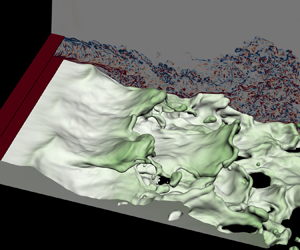
The temporal evolutions of the interfacial waves and the velocity fields for the cases W0 and W2 are shown in figure 3. The cases W0 and W2 represent the two distinct gas inflow conditions: laminar ( $I=0$) and highly turbulent (
 $I=0.13$). Figures 3(a) and 3(b) in the left column show the interfacial waves from a 3-D view, with the streamwise
  $u$-velocity in the background. Figures 3(c) and 3(d) in the right column are sequential snapshots of the gas–liquid interfaces coloured by the
  $u$-velocity from the top view.

Figure 3. Snapshots for the two-phase mixing layer for (a) the case W0 with a laminar gas inflow and (b) the case W2 with a turbulent gas inlet. The colour in the background in (a,b) represents the velocity magnitude. Temporal development of the interfacial waves for the cases W0 and W2 are shown in (c) and (d), respectively, where the colour at the interfaces represents the streamwise velocity. The frames in (c) and (d) are moving with the waves to keep the waves located at the centre of the window. Supplementary movies are available online at https://doi.org/10.1017/jfm.2021.481.
The results for the case W0 shown in figure 3(c) represent a typical process of interfacial wave formation and development for a planar two-phase mixing layer (Matas et al. Reference Matas, Marty and Cartellier2011; Agbaglah et al. Reference Agbaglah, Chiodi and Desjardins2017; Ling et al. Reference Ling, Fuster, Zaleski and Tryggvason2017; Zandian et al. Reference Zandian, Sirignano and Hussain2018; Ling et al. Reference Ling, Fuster, Tryggvasson and Zaleski2019). When the two streams meet at the end of the separator plate, the longitudinal instability is triggered due to the shear at the interface. The instability develops to a 2-D longitudinal interfacial wave which propagates downstream, the wave crest of which is approximately a straight line from the top view. Due to the transverse instability, the height of the wave crest varies over the transverse direction. When the wave amplitude grows, the wave interacts with the fast gas stream and develops into a 3-D wave, exhibiting a lobe shape. The liquid lobe later extends to form a liquid sheet which bends and folds. The thickness of the sheet reduces rapidly and unevenly due to the complex sheet deformation. Multiple holes are formed near the edge of the sheet. The expansion and merging of the holes disintegrate the liquid sheet violently. Multiple breakup events occur (see snapshots between  $t^{*}=335$ and 345 in figure 3c), until the sheet completely breaks into droplets.
By adding small-amplitude turbulent velocity fluctuations at the gas inlet (case W2), several important differences are observed. First of all, the longitudinal instability grows faster. As a result, the wave amplitude near the inlet is much higher than that for the laminar gas inflow. Second, the liquid sheet extending from the wave is much shorter, and experiences a weaker interaction with the gas stream. Third, the wavenumber of the transverse modulation of the interfacial wave increases. While there are approximately one to two transverse waves shown in figure 3(c) (see  $t^{*}=330$), approximately three to four waves are observed in figure 3(d) (see
  $t^{*}=350$). Due to the increase of wavenumber, the width of the lobes formed is reduced and the shape of the rim formed at the edge of the liquid sheet is less regular. Fourth, the breakup dynamics of the interfacial waves also changes significantly. Fewer holes are seen for the case W2. The disintegration of the wave takes a different path, i.e. forming fingers at the rim. Finally, the different breakup dynamic impacts the statistics of the droplets generated. Significantly fewer droplets are formed. Detailed quantitative analysis for these effects will be presented in the following sections.
3.2. Longitudinal instability and wave formation
3.2.1. Absolute instability
The shear between the gas and liquid streams triggers a Kelvin–Helmholtz (KH) longitudinal instability, which is the onset of the formation of interfacial waves. The temporal evolutions of the interfacial heights are measured near the inlet at  $x^{*}=0.625$ and eleven evenly spaced locations along the transverse direction. The temporal evolutions of the spatially averaged
  $h^{*}=h/H$ are shown in figure 4(a) for different cases of the wide and narrow domains. At this
  $x$ location, the wave amplitude is small (less than 4 % of
  $H$ for all cases), so the waves remain in the linear regime. Fourier transform is used to cast the temporal signals to the frequency spectra, see figure 4(b). The spectra obtained at eleven different transverse locations are averaged. The amplitude at the dominant frequency is the maximum in the spectra for all cases except W0, for which the dominant frequency is a local maximum. The maximum amplitude for the case W0 is located at a very low frequency that corresponds to the total simulation time.

Figure 4. (a) Temporal evolution of the transversely averaged interfacial heights at  $x^{*}=0.625$ for different cases. (b) Frequency spectra that correspond to temporal signal in (a). (c) Variation of the normalized dominant frequency for the longitudinal instability,
  $\omega _L^{*}/\omega _{L,0}^{*}$ as a function of
  $I$ for different cases, compared with the experimental data of Matas et al. (Reference Matas, Marty, Dem and Cartellier2015).
The appearance of the dominant mode affirms that the cases studied are in the absolute instability regime. The frequency of the longitudinal wave formation is dictated by the most-unstable mode of the longitudinal instability. As suggested by Matas (Reference Matas2015) and Matas et al. (Reference Matas, Delon and Cartellier2018), there are two different mechanisms that contribute to the convective-to-absolute instability transition: the surface tension and the confinement. Both types of absolute instabilities have been identified in the spatial-temporal stability analysis, as the pinching between the shear branch and the other branch controlled by surface tension (Otto et al. Reference Otto, Rossi and Boeck2013) or by confinement (Juniper Reference Juniper2006; Healey Reference Healey2007). For both types of absolute instability, the imaginary part of the frequency is positive at the pinch point. The wavenumber at the pinch point for the confinement type is generally low, so that the most-unstable wavelength is typically larger than the layer thickness  $H$. In contrast, for the surface-tension type, the wavenumber for the dominant mode is much higher and the corresponding wavelength is smaller than
  $H$. Another fundamental difference between the two is that the phase velocity at the pinch point for the confinement-triggered absolute instability follows the Dimotakis speed
  $U_D$, while the surface-tension absolute instabilities typically exhibit much smaller phase velocities.
The simulations for the cases with laminar gas inflows (N0 and W0) yield similar results for the dominant frequency and wavelength,  $\omega _L^{*} = 0.31$ and
  $\lambda ^{*} = 4.5$. Stability analysis without confinement for the same case has been performed in previous studies (Ling et al. Reference Ling, Fuster, Tryggvasson and Zaleski2019; Jiang & Ling Reference Jiang and Ling2020), which represent the absolute instability triggered by the surface-tension mechanism. The stability analysis slightly overestimates the dominant frequency
  $\omega ^{*}_{st}=0.40$, while the predicted wavelength
  $\lambda ^{*}_{st}=1.6$ is significantly lower than the simulation result, namely the surface-tension absolute instability over-predicted the wavenumber. Furthermore, it is found in the simulation results that, the wave propagation speed
  $U_w^{*}=0.22$, which agrees well with the Dimotakis speed and is much higher than the wave speed predicted by the surface-tension absolute instability,
  $U^{*}_{w,st}=0.10$. These discrepancies, together with the fact that
  $\lambda ^{*}>1$, seem to indicate the absolute shear instability observed here belongs to the inviscid confinement mechanism, instead of the surface-tension mechanism. Nevertheless, to fully confirm the nature of absolute instability, stability analysis similar to Matas (Reference Matas2015) needs to be performed, which will be relegated to our future work.
3.2.2. Dominant frequency
As shown in figure 4(b), when the gas inlet turbulence intensity  $I$ increases, the dominant frequencies shift to the right for both narrow and wide domains, and the amplitude also increases correspondingly. The normalized frequencies for different cases,
  $\omega _L^{*}/\omega _{L,0}^{*}$, where
  $\omega _{L,0}^{*}$ represents the frequency for
  $I=0$, are plotted in figure 4(c). The experimental data of Matas et al. (Reference Matas, Marty, Dem and Cartellier2015) are also shown for comparison. The experiments covered a wide range of injection conditions for different gas and liquid velocities, but the normalized frequencies approximately collapse. Although the simulation conditions are not identical to those for the experiments, the simulation results for the normalized frequency agree reasonably well with the experimental results. In particular, the general variation trend of
  $\omega _L^{*}/\omega _{L,0}^{*}$ over
  $I$ is well captured, i.e.
  $\omega _L^{*}/\omega _{L,0}^{*}$ varies little for
  $I\lesssim 0.02$ and increases with
  $I$ for
  $I\gtrsim 0.02$. The discrepancy between the simulation and experiment results may be due to the different density and viscosity ratios used in the present simulation.
The increase of  $\omega _L^{*}$ over
  $I$ can be explained by the viscous spatial-temporal stability analysis with eddy viscosity model (O'Naraigh, Spelt & Shaw Reference O'Naraigh, Spelt and Shaw2013; Matas et al. Reference Matas, Marty, Dem and Cartellier2015; Jiang & Ling Reference Jiang and Ling2020). The effective gas viscosity is the sum of the molecular and eddy viscosities, which increases with
  $I$ since the turbulent eddy viscosity increases with
  $I$. Furthermore, the Orr–Sommerfeld system indicated that the dominant frequency increases with the effective gas viscosity. When
  $I$ is small, the eddy viscosity is smaller than the molecular counterpart and that is why
  $\omega _L^{*}$ varies little for
  $I\lesssim 0.02$. More discussions on the stability analysis can be found in our previous study (Jiang & Ling Reference Jiang and Ling2020).
For similar  $I$,
$I$,  $\omega _L^{*}/\omega _{L,0}^{*}$ for the wide domain is smaller than that for the narrow domain. For example, the values of
  $I$ for the cases N3 and W1 are similar,
  $I_{N3}=0.056$ and
  $I_{W1}=0.06$, respectively, but
  $\omega _{L,W1}^{*}=0.38$ is approximately 9 % lower than
  $\omega _{L,N3}^{*}$. This seems to indicate that, the longitudinal instability is more sensitive to domain width when the gas inflow is turbulent. Since the turbulent gas flow is three-dimensional in nature, the small domain width may have constrained the development of the turbulence and the turbulence–interface interaction.
3.2.3. Spatial growth
The spatial development of the longitudinal instability determines the longitudinal growth of the interfacial wave amplitude. Since the interface motion will introduce a fluctuation in the liquid volume fraction  $c'=c-\langle \bar {c} \rangle$, the mean square of which, i.e.
  $\langle \overline {c'c'} \rangle$, is employed to measure the spatial longitudinal wave amplitude, see figure 5. For a given
  $x^{*}$, the vertical distance between the two contour lines of
  $\langle \overline {c'c'} \rangle =0.02$ is defined as the longitudinal wave amplitude
  $\xi _L^{*}$.

Figure 5. Spatial growth of the longitudinal wave amplitude (characterized by the mean square of liquid volume fraction fluctuations  $\langle \overline {c'c'}\rangle$, for the cases (a) W0, (b) W1 and (c) W2. The contour line
  $\langle \overline {c'c'} \rangle =0.02$ is used to measured the wave amplitude
  $\xi _L^{*}$.
It can be seen that,  $\xi _L^{*}$ grows rapidly with
  $x^{*}$ near the nozzle exit and this growth becomes more gradual downstream. From the log–linear plot shown in figure 6(a), the spatial growth of
  $\xi _L^{*}$ near the nozzle exit is approximately exponential, see e.g.
  $0.5\lesssim x^{*} \lesssim 0.8$ for the case W2. Nevertheless, it should be recalled that, since the longitudinal instability here is absolute, nonlinearity will influence the properties of the most-unstable mode and the spatial growth does not follow an exponential function as in convective instability (Otto et al. Reference Otto, Rossi and Boeck2013; Matas Reference Matas2015).

Figure 6. (a) The growth of the longitudinal wave amplitude  $\xi _L^{*}$ for different cases. The dotted lines indicate the spatial growth rate
  $\alpha ^{*}_L$ for different cases at
  $\log (\xi _L^{*})\approx -2$. (b) Variation of the normalized spatial growth rate
  $\alpha _L/\alpha _{L,0}$ as a function of
  $I$.
$I$.
As the inlet gas turbulence intensity  $I$ increases, the spatial growth of
  $\xi _L^{*}$, particularly near the nozzle exit, becomes faster. To characterize the effect of
  $I$, the spatial growth rate,
  $\alpha _L^{*}$, namely the slope of the curve
  $\log {\xi _L^{*}}$-
 $x^{*}$, is measured at
  $\log (\xi _L^{*})\approx -2$ for all cases. The variation of
  $\alpha _L^{*}$ over
  $I$ is shown in figure 6(b). Similar to the dominant frequency,
  $\alpha _L^{*}$ also increases with
  $I$. If a different threshold value for
  $\langle \overline {c'c'} \rangle$ other than 0.02 is to be used, the values of
  $\xi _L^{*}$ would change, but those for
  $\alpha _L^{*}$ will not be affected. For the cases W0 and N0, the variation
  $\xi _L^{*}$ over
  $x^{*}$ exhibits fluctuations, which makes the measurement of
  $\alpha _L^{*}$ somewhat sensitive. As will be discussed later in § 3.3.4, these fluctuations are induced by the spatial averaging over the transverse direction. To reduce the influence of the fluctuations, the measurement of
  $\alpha _L^{*}$ for the cases N0 and W0 is made for a wider range of
  $x^{*}$, as indicated in figure 6(a).
It can be observed from figure 6(a) that the values of  $\xi _L^{*}$ at the end of the separator plate,
  $x^{*}=\eta _x^{*}=0.5$, are almost zero for the narrow domain cases, but are finite for the wide domain cases. A snapshot of the interface near the inlet for the case W0 is shown in figure 7(a). The contact line where the three phases meet can be seen. A close-up in figure 7(c) shows that the contact line varies in time and also in the transverse direction. This indicates that the contact line moves on the separator front wall (facing the streamwise direction). Accurately capturing the contact-line dynamics is out of the scope of the present study. The boundary conditions on the solid separator plate are no-slip wall for velocity and symmetric for the liquid volume fraction
  $c$ (yielding a 90 degree contact angle). The small-amplitude spatial variation of the contact line is due to a numerical slip, with half of the cell size as the slip length (Snoeijer & Andreotti Reference Snoeijer and Andreotti2013). For the case N0, due to the constraint of the smaller domain width, the contact line remains a straight line pinned on the lower edge of the separator front wall, see figure 7(b). Therefore, when we compute the longitudinal wave amplitude by averaging
  $\overline {c'c'}$ in the transverse direction, the amplitude at
  $x^{*}=\eta _x^{*}$ for the case N0 is identical to zero, while that for the case W0 is finite.

Figure 7. (a) A close-up of the interface near the inlet and interfaces at  $x^{*}=\eta _x^{*}=0.5$ for different times for the cases (b) N0 and (c) W0. The interfaces for the case N0 collapse to a straight line.
Finally, it is worth mentioning that linear stability analysis has been performed in previous studies to identify the most unstable mode in the present configuration. Among the many attempts, the viscous spatial-temporal analysis has been shown to be quite successful (Otto et al. Reference Otto, Rossi and Boeck2013; Matas Reference Matas2015). The perturbation is introduced in the form of a 2-D normal mode. The resulting Orr–Sommerfeld equations are solved to obtain the most-unstable frequency and growth rate, which have been shown to agree well with the experimental and direct numerical simulation (DNS) results when the inlet gas is laminar (Fuster et al. Reference Fuster, Matas, Marty, Popinet, Hoepffner, Cartellier and Zaleski2013). In order to predict the most-unstable mode when turbulence is present at the gas inlet, additional modelling efforts are required. Attempts have been made by Matas et al. (Reference Matas, Marty, Dem and Cartellier2015) and Jiang & Ling (Reference Jiang and Ling2020) by incorporating the effect of inlet turbulence using the turbulent viscosity model. As the turbulent viscosity increases with  $I$, the Orr–Sommerfeld equations can reproduce the trends that the frequency increases with
  $I$. However, the modified stability model underestimates the values. The present simulation results indicate that the interface exhibits 3-D features right at the end of the separator plate, the assumption of 2-D mode in conventional stability analysis may need to be relaxed to yield better prediction.
3.3. Transverse instability and wave development
3.3.1. RT instability
Although the interfacial waves near the inlet are approximately longitudinal, transverse modulations are also observed, see figure 3. The transverse modulations are induced by the RT instability. As shown in figure 4, the longitudinal instability introduces oscillatory motion of the interface in the vertical direction. When the interface accelerates toward the liquid or decelerates toward the gas, the interface is unstable due to the baroclinic effect and the RT instability is triggered, see figure 8. While the longitudinal instability develops right at the end of the separator plate, the transverse interfacial modulation may not grow immediately, see figure 3(a). The reason is that the interface is stable in half time of one oscillation cycle (when the interface decelerates toward the liquid or accelerates toward the gas), see figure 8, so the transverse instability may first grow and then decay.

Figure 8. Schematic for the transverse RT instability due to the vertical motion of interface induced by the longitudinal instability.
The present results indicate that two conditions need to be satisfied for a transverse modulation to grow and to transform the 2-D longitudinal wave to fully three-dimensional. First, the longitudinal wave amplitude must be sufficiently large. Second, the interface is decelerating toward the gas, so that the growing interfacial wave will interact with the gas stream. A representative example of the development of the transverse instability is shown in figure 9. The later time evolution of this specific wave can be found in figure 3(c). At this time ( $t^{*}=323.75$) the interfacial wave is well aligned with transverse direction if viewed from the top, with some small transverse variations in the height of the wave crest. The interface is rising upward and decelerating toward the gas, the misalignment between the pressure and density gradients generates a baroclinic torque. The baroclinic torque in the
  $x$ direction,
  $B_x= (\nabla \rho \times \nabla p)_x$ will cause the transverse interfacial perturbation to grow, as indicated in figure 9(b), which shows the interface profile on the
  $y$–
$y$– $z$ plane. At this streamwise location
  $x^{*}\approx 1.6$, the amplitude of the longitudinal wave is large enough, as a result, the wave crest will experience a significant interaction with fast gas stream above the wave. The local acceleration of the gas flow above the wave crest creates a Bernoulli depression, which will further pull the interface upward (Hoepffner et al. Reference Hoepffner, Blumenthal and Zaleski2011), amplifying the transverse modulation of the interface, see
  $t^{*}=322.5$ to 327.5 in figure 3(c). More discussions about the interaction between the interfacial wave and the gas stream will be presented in § 3.4.1.

Figure 9. Transverse development of the RT instability for the case W0. (a) Top view of the interface at  $t^{*} = 323.75$, and the interface is coloured with
  $u$-velocity (m s
 $^{-1}$). The vertical dashed line in (a) indicates the wave location, and the interface profile along the dashed line is shown in (b) on the
  $y-z$ plane to demonstrate the baroclinic effect.
3.3.2. Dominant mode for transverse instability
Although the transverse modulation growth is assisted by its interaction with the gas stream, the selection of the dominant transverse wavenumber is mainly controlled by the RT instability. The inviscid linear temporal RT instability with surface tension for a planar interface yields the following dispersion relation (Chandrasekhar Reference Chandrasekhar1961):
 \begin{equation} \omega_I = \left(ak\frac{\rho_l-\rho_g}{\rho_l+\rho_g}- \frac{\sigma k^{3}}{\rho_l+\rho_g}\right)^{1/2}, \end{equation}
where  $\omega _I$ is temporal growth rate,
  $k$ is wavenumber and
  $a$ is magnitude of the interfacial acceleration. To account for the viscous effect, the dispersion relation becomes (Chandrasekhar Reference Chandrasekhar1961; Joseph, Belanger & Beavers Reference Joseph, Belanger and Beavers1999)
 \begin{equation} \omega_I ={-}k^{2} \frac{\mu_l+\mu_g}{\rho_l+\rho_g}\pm \left(ak\frac{\rho_l-\rho_g}{\rho_l+\rho_g}- \frac{\sigma k^{3}}{\rho_l+\rho_g}+ k^{4} \left(\frac{\mu_l+\mu_g}{\rho_l+\rho_g}\right)^{2} \right)^{1/2}. \end{equation}
Due to the low liquid viscosity in the present problem, the viscous effect on the RT instability is very small. The difference between (3.1) and (3.2) is negligible, so the inviscid relation (3.1) will be used in the following analysis.
Based on (3.1), the transverse wavenumber for the most unstable mode is
 \begin{equation} k_{T}=\sqrt{\frac{a(\rho_l-\rho_g)}{3\sigma}}, \end{equation}
and the corresponding growth rate is
 \begin{equation} \omega_{T}=\frac{2}{3^{3/2}} \left( \frac{a^{3}(\rho_l-\rho_g)}{\sigma}\right)^{1/4}. \end{equation}
 The interfacial acceleration  $a$ is induced by the longitudinal instability, for which the characteristic length and time scales are
  $\delta$ and
  $1/\omega _L$, respectively. Therefore, it can be approximated that
  $a\sim \delta \omega _L^{2}$ and the dominant transverse wavenumber
 \begin{equation} k_{T}\approx \omega_L\sqrt{\frac{\delta (\rho_l-\rho_g)}{3\sigma}}. \end{equation}
As shown in § 3.2,  $\omega _L$ increases with
  $I$. According to (3.5),
  $k_T$ will also grow with
  $I$.
$I$.
Using similar scaling relations, the temporal growth rate for the transverse instability can be estimated as
 \begin{equation} \omega_{T} \approx \frac{2}{3^{3/2}} \left( \frac{\delta^{3} \omega_L^{6}(\rho_l-\rho_g)}{\sigma}\right)^{1/4}. \end{equation}
Since  $\omega _L \sim U_D/\delta$, it can be shown that
 \begin{equation} {\omega_{T}} \approx \omega_L We_{L}^{1/4}, \end{equation}
where  $We_L$ is the Weber number for the longitudinal wave, expressed as
 \begin{equation} We_L = \frac{(\rho_l-\rho_g)U_D^{2} \delta}{\sigma}. \end{equation}
If  ${\omega _{T}}$ is significantly lower than
  ${\omega _L}$, then the RT instability will not grow fast enough to be relevant. For the present problem,
  $We_L=9.45$, and it is estimated that
  ${\omega _{T}}/{\omega _L} \sim$ O(1). Therefore, the time scales for the longitudinal KH and the transverse RT instabilities are comparable. In other words, the transverse RT instability can grow in a time scale that is comparable to oscillatory interface motion induced by the longitudinal instability. This affirms that RT instability is responsible to the transverse development of the interfacial waves for the present problem.
3.3.3. Transverse wavenumber spectra
To investigate the effect of inlet gas turbulence intensity  $I$ on the dominant transverse wavenumber, the wavenumber spectrum of the transverse interfacial modulation is examined. For a given
  $t^{*}$ and
  $x^{*}$, a Fourier transform is performed for the interfacial height
  $h$ along the transverse direction. Then, the wavenumber for the maximum amplitude in the spectrum,
  $k_{max}$, is measured. The contours of
  $k_{max}$ for different
  $I$ are shown in figure 10.

Figure 10. The dominant transverse wavenumber  $k_{max}$ on the
  $x^{*}$–
 $t^{*}$ diagrams for the cases (a) W0, (b) W1 and (c) W2. The vertical dashed lines indicate the streamwise locations to estimate the time-averaged transverse wavenumber
  $\bar {k}_T$.
It is observed that  $k_{max}$ rises to much larger values when longitudinal waves pass by. This suggests that the development of the transverse modulations is closely associated with the longitudinal waves, as predicted by the stability analysis (3.5). As a result, the
  $k_{max}$ contours also reveal important features about the formation and propagation in the longitudinal waves. First of all, the trajectories of the longitudinal waves appear as inclined straight lines of higher
  $k_{max}$ values in the figures. The slopes of the lines represent the wave propagation speeds in the longitudinal direction. It is observed that the wave speeds are very similar for all the cases and agree with the Dimotakis speed (Dimotakis Reference Dimotakis1986),
  $U_D$. For the present problem,
  $U_D^{*}=U_D/U_g=0.223$. As the longitudinal wave grows in amplitude and interact with the fast gas stream, the aerodynamic drag will cause the wave to accelerate. That is why the longitudinal wave trajectories bend downward slightly further downstream, which is most profound for the case W2 due to the faster spatial growth for the longitudinal instability, see figure 10(c). The time period
  $\tau _L$ and the wavelength
  $\lambda _L$ for the longitudinal waves can also be identified, and they are related by
  $U_D$ as
  $\lambda _L =U_D \tau _L$. It is also observed that
  $\tau _L$ decreases with
  $I$. Since
  $U_D$ remains unchanged,
  $\lambda _L$ decreases with
  $I$.
$I$.
It is noted that only  $k_{max}$ on the longitudinal wave location characterizes the transverse modulations of the interfacial waves. Between two longitudinal waves,
  $k_{max}$ represents the ripples on the interfaces, which are less important. Therefore, we denote the
  $k_{max}$ at the passages of the longitudinal waves as the transverse wavenumber of the interfacial wave,
  $k_T$. It is observed that
  $k_{T}$ for different waves are different due to the chaotic nature of the turbulent multiphase flows. The temporal evolution of
  $k_{max}$ for different
  $I$ is shown in figures 11(a)–11(c). For each case, the measurement is made at
  $x^{*}$ locations corresponding to
  $\log (\xi _L^{*})=-1$, i.e.
  $x^{*}=2.375$, 1.625, 1.25, for the cases W0, W1 and W2, respectively, which are indicated by dashed lines in figure 10. The RT instability predictions (3.5) are also shown in figure 11 for comparison. It can be observed that
  $k_{T}$ generally increases when
  $I$ increases, which is consistent with the RT instability theory. The increase of
  $k_T$ with
  $I$ is also consistent with the snapshots shown in figure 3.

Figure 11. Temporal evolution of transverse wavenumber  $k_{max}$ for the cases (a) W0 at
  $2.375H$, (b) W1 at
  $1.625H$ and (c) W2 at
  $1.25H$. The vertical lines indicated the passage times of the longitudinal waves, which are estimated based on the
  $\omega _L$ for the corresponding
  $I$. (d) Variation of
  $\bar {k}_{T}$ with turbulent intensity
  $I$, compared with the RT predictions (3.5).
The time-averaged transverse wavenumber  $\bar {k}_{T}$ is plotted as a function of
  $I$ in figure 11(d). The measurement times for
  $k_{T}$ are indicated by the vertical lines in figures 11(a)–11(c), which correspond to the longitudinal wave passage times estimated based on the dominant longitudinal frequency
  $\omega ^{*}_L$ for the given
  $I$. It is shown that
  $\bar {k}_T$ increases from approximately 3330 to 5100 when
  $I$ increases from 0 to 0.13. The values of
  $\bar {k}_T$ for
  $I=0$ and 0.13 correspond to approximately 2.5 and 3.9 waves in the domain width. The RT instability model (3.5) well captures the increasing of trend of
  $\bar {k}_T$ over
  $I$. The discrepancy between the model predictions and the simulation results can be up to 17 %, so the model predictions can only be used as approximations of
  $\bar {k}_T$.
3.3.4. Transverse modulation amplitude
The wave amplitude for a given  $(x^{*},z^{*})$ location can be characterized by the root mean square of the interfacial height fluctuations normalized by
  $H$, i.e.
  $\xi ^{*}=(\overline {h'h'})^{1/2}/H$. The variations of
  $\xi ^{*}$ with
  $x^{*}$ and
  $z^{*}$ for different cases are shown in figure 12. The wave amplitude generally increases in the longitudinal direction, although small variations in the transverse direction are also observed. It should be noted that
  $\xi ^{*}$ can be used to characterize the wave amplitude only when the wave amplitude is small. The noise observed in figure 12(c) is due to the rolling up and breakup of the waves. The transverse variations are the most profound for the case W0.

Figure 12. Spatial variation of the interfacial wave amplitude  $\xi ^{*}=(\overline {h'h'})^{1/2}/H$ for the cases (a) W0, (b) W1 and (c) W2.
If  $\xi ^{*}$ is averaged in the transverse direction, we can obtain the longitudinal wave amplitude, i.e.
  $\check {\xi }_L = \langle (\overline {h'h'})^{1/2}/H\rangle$. The spatial variation of
  $\check {\xi }_L$ in
  $x^{*}$ direction is shown in figure 13(a). The results for the longitudinal wave amplitude
  $\xi _L^{*}$ defined based on the contours of
  $\langle \overline {c'c'}\rangle =0.02$ (see figure 5a) are also shown for comparison. It can be observed that, although the values for
  $\check {\xi }_L$ and
  ${\xi }_L^{*}$ are different, the ratio
  $\check {\xi }_L/{\xi }_L^{*}$ is approximately a constant for all cases. Therefore, the spatial growth rates for the longitudinal instability
  $\alpha _L^{*}$ will remain the same, no matter if
  $\check {\xi }_L$ or
  ${\xi }_L^{*}$ is used. The curve of
  $\check {\xi }_L$ for the case W0 exhibits some fluctuations, which are due to stronger transverse variations of
  $\xi ^{*}$. The results of
  $\xi ^{*}$ at different transverse locations are shown in figure 14. It can be observed that the
  $\xi ^{*}$-
 $x^{*}$ curves are very different for the case W0, while the difference among different profiles is much smaller for the cases W1 and W2. In spite of the different
  $\xi ^{*}$-
 $x^{*}$ curves at different transverse locations for the case W0, the growth rates
  $\alpha _{L,W0}^{*}$ are quite similar, see figure 14(a). Therefore, the measurement of
  $\alpha _L^{*}$ for the case W0 is not as uncertain as it may appear in figures 6(a) and 13(a).

Figure 13. Spatial variation of (a) longitudinal wave amplitude  $\check {\xi }_L$ and (b) transverse modulation amplitude
  $\check {\xi }_T$ along the
  $x^{*}$ direction for the cases W0, W1 and W2. The results for the longitudinal wave amplitude
  $\xi _L^{*}$, which are measured based on the liquid volume fraction fluctuations
  $\langle \overline {c'c'}\rangle$, are also shown in (a) for comparison.

Figure 14. Spatial variation of wave amplitude  $\xi ^{*}$ at different
  $z$ locations for the cases (a) W0, (b) W1 and (c) W2.
For a given  $x^{*}$, the deviation of wave amplitude
  $\xi ^{*}$ from the transverse mean
  $\check {\xi }_L$ can be calculated as
  $\xi ^{*}-\check {\xi }_L=(\overline {h'h'})^{1/2}/H-\langle (\overline {h'h'})^{1/2}/H \rangle$. Then, the root mean square of the deviation,
  $\check {\xi }_T=\langle (\xi ^{*}-\check {\xi }_L)^{2}\rangle ^{1/2}$, can be used to characterize the average amplitude of the transverse modulations, which is plotted as a function of
  $x^{*}$ in figure 13(b). Near the inlet,
  $\check {\xi }_T$ is at least an order of magnitude smaller than
  $\check {\xi }_L$ (
 $\check {\xi }_L/\check {\xi }_T \gtrsim \exp (2.5$)). As the longitudinal wave amplitude grows in
  $x^{*}$, the transverse modulation amplitude also grows correspondingly. The spatial growth rates of
  $\check {\xi }_T$ near the inlet are similar for different
  $I$. Yet since the spatial growth of
  $\check {\xi }_L$ is higher for larger
  $I$, the wave amplitude exceeds the linear regime at a smaller
  $x^{*}$. Beyond that point, the interfacial waves start to deform and break, then
  $\check {\xi }_T$ is not valid to characterize the transverse modulation amplitude. For the case W0, since the longitudinal wave grows more slowly,
  $\check {\xi }_T$ has a wider
  $x^{*}$ range to grow, reaching a higher value than for the cases W1 and W2.
3.4. Development and disintegration of 3-D interfacial waves
3.4.1. Wave–gas-stream interaction
When the wave amplitude grows beyond the linear regime, such as  $\xi ^{*}>0.1$, the nonlinear interaction between the interfacial wave and the fast gas stream will influence the subsequent deformation of the wave and the liquid sheet extended from the wave crest. The temporal evolutions of the interfaces, the pressure and the velocity magnitude for the case W0 are shown in figure 15. The first snapshots at
  $t^{*}=327.5$ correspond to approximately the end of the linear regime, and the interfacial wave appears like a lobe of small amplitude. The continuous growth of the wave introduces perpendicular exposure of the wave crest to the fast gas stream. As a consequence of that, a high pressure is built up on the upstream side of the wave, see figure 15(b). The gas flow accelerates over the wave crest, introducing a low pressure above due to the Bernoulli principle. Furthermore, the gas flow separates on the downstream side (see figure 15c), which also introduces a low pressure wake region. The pressure difference leads to an aerodynamic drag that pushes the wave crest upward and also along the streamwise direction, further destabilizing the interfacial wave. As a consequence of that, a liquid sheet is extended from the wave crest, see figure 15(a) at
  $t^{*}=332.5$. The Taylor–Culick rim is formed on the edge of the liquid sheet. It can be observed that the rim is not as smooth as that at the earlier time and exhibits transverse variation with a higher wavenumber. Multiple mechanisms contribute to the secondary transverse variations of the wave shape. At first, another RT instability is triggered due to the acceleration of the rim in the longitudinal direction. Furthermore, the RP instability of the rim can also lead to variation in the rim diameter. Finally, the turbulent wake of the wave and the interaction between the turbulent vortices and the liquid sheet can also cause irregular deformation of the liquid sheet.

Figure 15. Temporal evolutions of the (a) interfaces, (b) pressure and (c) velocity magnitudes for the case W0, to demonstrate the interaction between the interfacial wave and the gas stream. The interfaces in (a) are coloured by the streamwise velocity. The pressure and velocity shown in (b,c) are on the  $x$–
$x$– $y$ plane through the wave. The frame is moving with the wave to keep the wave located at the centre of the window.
As the interfacial wave continues to grow, the interaction with the gas stream becomes more intense and complex. The liquid sheet starts to bend and fold. The thickness of the liquid sheet at the folding region becomes very small and, as a result, holes are formed in the liquid sheet. In figure 15(a), it can be observed that, at  $t^{*}=337.5$, the folded segment of the liquid sheet has completely broken, forming droplets and filaments of different sizes. A new rim will form at the edge of the unbroken sheet that remains attached to the wave, and another cycle of wave–gas-stream interaction will occur. Yet as the interfacial wave is now further away from the inlet and the velocity of the gas stream decreases along the streamwise direction due to turbulent dissipation, the subsequent interaction between the interfacial wave and the gas stream will be less intense.
3.4.2. Hole formation and sheet disintegration
The formation and development of the holes in the liquid sheet for the cases W0 and W2 are shown in figure 16. The  $w$-velocity is shown on the interfaces and also on the cross-section
  $y-z$ planes at the hole centres. As can be seen in figure 16(a), at
  $t^{*}=246.25$, the thickness of the liquid sheet is highly uneven due to the sheet deformation. Furthermore, it can be observed that the liquid is moving away from location of minimum thickness (see figure 16a at
  $t^{*}=246.25$). Eventually the two surfaces pinch and a hole is formed. The pinching process observed here is reminiscent of pinching of liquid neck in drop formation (Castrejón-Pita et al. Reference Castrejón-Pita, Castrejón-Pita, Thete, Sambath, Hutchings, Hinch, Lister and Basaran2015; Zhang et al. Reference Zhang, Ling, Tsai, Wang, Popinet and Zaleski2019). After the holes are formed, the Taylor–Culick (TC) rim develops on the edge of the hole. Due to the capillary effect, the rim retracts radially, making the holes expand. The speed of hole expansion is dictated by the rim retraction velocity, namely the TC velocity,
 \begin{equation} U_{TC}=\sqrt{\frac{2\sigma}{\rho e}}, \end{equation}
where  $e$ is the liquid sheet thickness. The curvature of the rim has little effect on the retraction velocity (Agbaglah Reference Agbaglah2021). Since the thickness of the liquid sheet is non-uniform,
  $e$ varies from
  $14.2$ to
  $6.5$
$6.5$  $\mathrm {\mu }$m near the edge of the hole, see figure 16(a) at
  $t^{*}=247.5$, for which the hole expansion velocity predicted by theory (3.9) is 0.84–1.24 m s
 $^{-1}$. The hole expansion velocity measured from the simulation results is approximately 1.35 m s
 $^{-1}$, which is in reasonable agreement with the TC predictions. When the inlet gas is turbulent, the gas flow around the sheet exhibits more intense fluctuations, which can be recognized from the footprints on the interfacial velocity (see figure 16b). The surrounding turbulence seems to have little effect on the hole expansion speed, which is found to be similar to that for the case W0. This indicates that the capillary effect still dominates the hole development. Nevertheless, it is observed that the hole is formed closer to the rim. As a result, the expansion of the hole will interact with the rim and cause the rim to break (Agbaglah Reference Agbaglah2021).

Figure 16. Formation and development of holes in liquid sheets for the cases (a) W0 and (b) W2. The  $w$-velocity is plotted on the interfaces and also on the cross-section
  $y-z$ planes at the hole centres (indicated by the dashed lines). The frame is moving with the hole to keep the hole located at the centre of the window.
3.4.3. Impact of inlet gas turbulence on sheet breakup
Although the inlet gas turbulence does not change the hole dynamics, it does have a strong impact on the number of holes formed, and the locations where the holes are formed. The breakups of the liquid sheet for the W0 and W2 cases are shown in figure 17. For the case W0, the holes are formed at around  $x^{*}=4.275$, which is much further than the hole formation location
  $x^{*}=3.025$ for the turbulent gas inlet. This is due to smaller growth rate for the case W0, and as a result, the interaction between the wave and the gas stream occurs further downstream. Nevertheless, the interfacial wave for the case W0 reaches a larger amplitude and experiences a stronger interaction with the gas stream. Furthermore, the interfacial wave is accelerated by the gas stream to a higher velocity and is stretched to form a longer liquid sheet. The folding of the liquid sheet enhances the reduction of sheet thickness (see also figure 15). Multiple holes arise and expand simultaneously and the merging of the holes leads to a violent breakup of the folding segment of the liquid sheet (Agbaglah Reference Agbaglah2021). The rim of the liquid sheet is detached from the wave, forming a filament aligned with the transverse direction, see
  $t^{*}=238.75$ in figure 17(a). The detached filament interacts with the gas stream and continues to break into droplets. Due to the irregular shape of the filament, the breakup dynamics is different from the regular Rayleigh breakup of a perturbed liquid cylinder (Villermaux et al. Reference Villermaux, Marmottant and Duplat2004).

Figure 17. Breakups of the liquid sheet due to hole formation and development for the cases (a) W0 and (b) W2. The interfaces are coloured with  $u$-velocity.
For the case W2, the transverse wavenumber is higher than that for the case W0. Therefore, the interfacial wave exhibits narrower lobes and more irregular rims. In the snapshots shown in figure 17(b), only one hole is seen. By examining all the time snapshots, it is confirmed that the number of holes formed for the case W2 is significantly lower than that for the case W0. Since only one hole is formed, instead of merging with other holes as for the case W0, the hole expands and merges with the rim. The rim eventually breaks and retracts to form two fingers aligned with the longitudinal direction. The fingers are stretched by the gas stream and will break and form droplets. Since the size and orientation of the fingers/filaments formed for the case W2 are distinct from those for the case W0, the resulting droplet statistics will also be different.
3.5. Droplet statistics
To obtain statistics of droplets formed in the interfacial wave breakup, the cells with liquid ( $f>0$) that are connected together are tagged with the same identity. Then, the volume and centroid coordinates of individual liquid structures can be computed. The details of the tagging approach can be found in a previous study (Ling et al. Reference Ling, Zaleski and Scardovelli2015).
3.5.1. Size distribution
The droplet size distribution for different cases are shown in figure 18. Only the droplets in the region  $x^{*}<14$ are considered, to exclude the effect of the outflow boundary. Furthermore, sampling is only performed after the droplet statistics have reached the statistically stationary state (at approximately
  $t^{*}=200$). For all cases, droplets are collected every 50 time steps, so in total approximately
  $N_s=3000$ samples have been collected. The sampling time has been verified to be sufficiently long to yield statistically converged results. Since the droplet number generally decreases with the droplet diameter
  $d$, the size interval
  $\Delta d$ is increased over
  $d$ with a scaling ratio 1.15, namely
  $\Delta d_{i+1} = 1.15 \Delta d_{i}$, where
  $i$ is the interval number. The number of droplets falling into the size interval centred with the diameter
  $d$ for all samples is denoted as
  $n$. The average droplet number is then defined as
  $\bar {n}=n/N_s$.

Figure 18. (a) Droplet size distribution and (b) PDF based on the time-averaged droplet number for the cases W0, W1 and W2.
The results for  $\bar {n}$ as a function of
  $d$ for the cases W0, W1 and W2 are shown in figure 18(a). It is observed that
  $\bar {n}$ for all
  $d$ generally decreases when
  $I$ increases. This is consistent with the observation in figure 17, namely, that the interfacial wave breakup is less violent when
  $I$ increases, and as a result, fewer droplets are formed. Nevertheless, the shapes of the distribution profiles for different
  $I$ are quite similar, which motivates the examination of the probability density function (PDF). The droplet size PDF based on the droplet number is defined as
 \begin{equation} P_n(d)= \frac{\bar{n}(d)}{\Delta d\displaystyle\sum \bar{n}(d)}. \end{equation}
 The droplet size PDFs for different  $I$ are shown in figure 18(b). The profile of
  $P_n$ is quite complex and cannot be represented by any typical distribution function. The recent study by Balachandar et al. (Reference Balachandar, Zaleski, Soldati, Ahmadi and Bourouiba2020) indicates that a combined log–normal and Pareto distribution is required to represent the complex PDF for the respiratory droplets formed in a coughing event (Duguid Reference Duguid1946). While the small droplets follow the log–normal distribution, the larger droplets follow the Pareto distribution. The drop size PDFs for the present problem for different ranges of droplet size also seem to follow different distribution functions, i.e. the log–normal, Pareto and exponential distribution functions. The expressions for these three functions are given as
 $$\begin{gather} P_L(d) = \frac{B_L}{{d \hat{\sigma} \sqrt{2{\rm \pi}}}} \exp \left[ -\frac{(\ln d -\hat{\mu})^{2}}{2\hat{\sigma}^{2}}\right], \end{gather}$$
 $$\begin{gather}P_P(d) = \frac{B_P}{d^{\alpha}}, \end{gather}$$
 $$\begin{gather}P_E(d) = B_E \exp(d/\lambda), \end{gather}$$
where  $B_L$,
  $B_P$ and
  $B_E$ are the corresponding normalization constants for the log–normal, Pareto and exponential functions, respectively. For the log–normal function,
  $\hat {\mu }$ and
  $\hat {\sigma }$ are the expected value and the standard deviation of
  $\ln d$. While
  $\alpha$ is the power index for the Pareto distribution,
  $\lambda$ is the characteristic length for the exponential distribution. To compare the simulation results with the distribution functions, we have used the data for the case W1 to fit these distributions functions. For convenience of discussion, the droplets for
  $d \lesssim 25$
  $\mathrm {\mu }$m,
  $25\lesssim d \lesssim 140$
  $\mathrm {\mu }$m and
  $d \gtrsim 140$
  $\mathrm {\mu }$m are referred to as small, medium and large droplets, the data of which are used to fit (3.11), (3.12) and (3.13), respectively. The boundaries between different ranges vary slightly with
  $I$. The values for the fitting parameters are
  $B_L=1.14$,
  $\hat {\sigma }=0.35$,
  $\hat {\mu }=2.24$ for the log–normal function,
  $B_P=0.099$,
  $\alpha =1.04$ for the Pareto function and
  $B_E=0.0035$,
  $\lambda =95.0$ for the exponential function. The units for these parameters can be determined based on the units for
  $P_n$ and
  $d$, i.e. (
 $\mathrm {\mu }$m)
 $^{-1}$ and
  $\mathrm {\mu }$m, respectively. As shown in figure 18(b), the fitted distribution functions generally agree well with the simulation results.
For the large droplets ( $d \gtrsim 140$
  $\mathrm {\mu }$m), the curves of
  $P_n$ for different
  $I$ approximately collapse to the same exponential function. The exponential tail in the drop size distribution has been observed in numerous experiments and simulations (Simmons Reference Simmons1977a,Reference Simmonsb; Marmottant & Villermaux Reference Marmottant and Villermaux2004; Ling et al. Reference Ling, Zaleski and Scardovelli2015). For droplets of medium size,
  $25 \lesssim d \lesssim 140$
  $\mathrm {\mu }$m, the PDF exhibits a power-law decay, namely the Pareto distribution. The width of the Pareto distribution region increases with the the inlet gas turbulence intensity
  $I$. As a result, the power-law decay is the most profound for the case W2. For the small droplets
  $d \lesssim 25$
  $\mathrm {\mu }$m, the shape of
  $P_n$ is significantly different from that for the medium droplets. The different PDF profiles may be due to the different droplet formation mechanisms. While the large number of small droplets are probably generated directly in the breakup of liquid sheets, see figure 17(a), the medium droplets are produced in the RP breakup of thicker ligaments and fingers, see figure 17(b). It will be interesting for future study to identify
  $P_n$ for different breakup events and to further reveal the physical reasons behind the different
  $P_n$ for the small and medium droplets. Following former studies (Marty Reference Marty2015; Ling et al. Reference Ling, Fuster, Zaleski and Tryggvason2017; Balachandar et al. Reference Balachandar, Zaleski, Soldati, Ahmadi and Bourouiba2020), the log–normal function has been used to fit
  $P_n$ for the small droplets, although the narrow range of
  $d$ may have placed some uncertainty in the fitting process and whether the log–normal function is indeed the best fit for the small droplets. It should be noted that the droplets smaller than 8
  $\mathrm {\mu }$m are not accounted here, since those droplets are smaller than approximately one cell and the formation of these droplets is likely under-resolved. To better examine the distribution function for the small droplets, more data points are required for
  $d<8$
$d<8$  $\mathrm {\mu }$m, which would require further refined simulations. Such simulations require computer time at least an order of magnitude higher than that for the present simulations and will be relegated to future works.
3.5.2. Spatial distribution
The spatial distributions of droplet number  $\bar {n}$ in the longitudinal and vertical directions for different droplet size ranges and the cases W0, W1 and W2 are shown in figure 19. In the longitudinal direction,
  $\bar {n}$ is zero until the interfacial waves break. After that,
  $\bar {n}$ increases with
  $x^{*}$, approximately following the hyperbolic tangent function, see figure 19(a). For the small and medium droplets,
  $\bar {n}$ reaches the maximum around
  $10\lesssim x^{*}\lesssim 13$. The decrease in
  $\bar {n}$ for
  $x^{*}\gtrsim 13$ is due to the coalescence of droplets and the merger of droplets back on the unbroken liquid layer at the bottom (see figure 3c,d). For large droplets, the decrease of
  $\bar {n}$ is less profound, and
  $\bar {n}$ reaches a plateau for large
  $x^{*}$. When the inlet gas turbulence intensity
  $I$ increases, several changes are induced. First, the onset of the increase of
  $\bar {n}$ occurs at smaller
  $x^{*}$ due to the faster growth of the longitudinal wave and the earlier breakup of the interfacial waves. Second, the increase of
  $\bar {n}$ becomes more gradual and eventually settles on a lower plateau. As a result, the curves for W0 and W1 cross at a critical longitudinal location
  $x^{*}_c$. For
  $x^{*}< x^{*}_c$,
  $\bar {n}_{W1}> \bar {n}_{W0}$, or vice versa. The values of
  $x^{*}_c$ for the small and medium droplets are similar, at approximately
  $x^{*}_c=7$, while that for the large droplets is larger, at approximately
  $x^{*}_c=8.2$.

Figure 19. Distribution of  $\bar {n}$ in (a) streamwise and (b) vertical directions for the cases W0, W1 and W2. The droplets are collected every 50 time steps. The three columns are for the small (12.5–100
  $\mathrm {\mu }$m), medium (100–200
  $\mathrm {\mu }$m) and large (200–300
  $\mathrm {\mu }$m) droplets, respectively.
The droplet number distributions in the vertical direction for different droplet size ranges are shown in figures 19(d)–19( f). For the small droplets, the maxima of  $\bar {n}$ are at the bottom plane of the domain for all cases. The droplet number then decreases rapidly with
  $y^{*}$ until
  $y^{*}\approx 1$, where the interface is located at the inlet and the decrease of
  $\bar {n}$ becomes more gradual. After that,
  $\bar {n}$ decreases approximately exponentially to zero, see figure 19(d). The accumulation of small droplets near the bottom domain is probably due to the fact that the small droplets have smaller inertia and thus are easier to be carried by the gas stream toward the bottom downstream. The medium and larger droplets have larger inertia and tend to maintain the velocity direction when they are formed. As a result, we see the maxima of
  $\bar {n}$ for the medium and the large droplets are near
  $y^{*}=1$, instead. The vertical location corresponding to the maximized
  $\bar {n}$ is denoted by
  $y^{*}_{max}$ (see figure 19e). It is observed that, for the medium and large droplets,
  $y^{*}_{max}$ decreases with the inlet gas turbulence intensity
  $I$. This is again due to the faster growth of the longitudinal wave for the cases with larger
  $I$, and as a result, the breakups of the interfacial waves occur in a lower vertical location (see also figure 3).
4. Conclusions
The effect of inlet gas turbulence on the formation, development and breakup of the interfacial waves in a two-phase mixing layer is investigated through direct numerical simulation. The gas and liquid properties and the mean injection velocities are chosen to place the present case in the absolute instability regime. Turbulent velocity fluctuations are induced at the gas inlet and a parametric study for the inlet gas turbulence intensity  $I$ is performed. The governing equations are solved using the open-source multiphase flow solver, PARIS, in which the mass–momentum consistent VOF method is used to capture the sharp gas–liquid interfaces. To allow a detailed investigation of the transverse development of the interfacial waves, two different domain widths have been used. The wide domain consists of approximately 1.6 billion cells.
The temporal evolutions and the frequency spectra for the interfacial height in the near field show a dominant frequency, confirming that the case is in the absolute instability regime. The dominant frequency varies little when  $I\lesssim 0.02$ but then increases over
  $I$ after the threshold. A similar increasing trend over
  $I$ has been observed for the spatial growth rate of the longitudinal wave amplitude. When the inlet gas is laminar, the dominant frequencies and spatial growth rates for the narrow and wide domains are similar. When the turbulence is present at the gas inlet, deviations between the results for the narrow and wide domains are observed.
The longitudinal instability introduces vertical motion of the interface. When the interface moves upward and decelerates toward the gas, the RT instability is triggered, introducing transverse modulations on the interfacial waves. The transverse variation is amplified as the wave interacts with the fast gas stream. The selection of dominant transverse wavenumber is dictated by the RT instability and can be determined by inviscid temporal stability theory with surface tension. The transverse wavenumber scales with the longitudinal frequency and thus will also increase with  $I$. The simulation results for the transverse wavenumber agree well with theoretical predictions. The growth rate of the transverse instability is estimated to be comparable to the dominant frequency of the longitudinal instability, affirming the RT instability is responsible for the initiation of the transverse modulations for the present problem.
The subsequent development of the interfacial wave is controlled by the nonlinear interaction with the gas stream. When the interfacial wave invades the gas stream, an aerodynamic drag is developed, which further destabilizes the interfacial waves and stretches the wave crest to form liquid lobes/sheets. For the laminar gas inlet, the liquid sheet deforms and folds when it interacts with the gas stream, leading to the formation of multiple holes in the folding area. The expansion and merging of the holes eventually lead to a violent disintegration of the liquid sheet, detaching filaments that are aligned with the transverse direction. In contrast, for the turbulent gas inlet, the lobes are narrower and the rim is less regular. Fewer holes are formed and the expansion of the holes interacts with the rim, forming fingers aligned with the longitudinal direction. The different breakup dynamics of the liquid sheet results in different sizes and orientations of the filaments. The droplets formed due to the subsequent breakup of the filaments thus exhibit different statistics.
The numbers of droplets for all sizes are reduced when  $I$ increases, although the PDFs appear to be similar. The droplets of different size ranges are found to follow different distribution functions, i.e. the log–normal, Pareto and exponential functions for the small (
 $8 \lesssim d \lesssim 25$
  $\mathrm {\mu }$m), medium (
 $25 \lesssim d \lesssim 140$
  $\mathrm {\mu }$m) and large (
 $d \gtrsim 140$
  $\mathrm {\mu }$m) droplets, respectively. The spatial distributions of the droplet number for different size ranges have also been presented. The increase of the droplet number along the longitudinal direction is similar to the hyperbolic tangent function and the decrease of droplet number along the vertical distance away from the mixing layer follows the exponential function. When
  $I$ increases, more droplets are formed in the near field and near the bottom of the domain.
Supplementary movies
Supplementary movies are available at https://doi.org/10.1017/jfm.2021.481.
Acknowledgements
We also thank Dr G. Tryggvason, Dr S. Zaleski and other developers of for their contributions to the PARIS solver.
Funding
This research is supported by the National Science Foundation (No. 1942324). The authors also acknowledge the Extreme Science and Engineering Discovery Environment (XSEDE) for providing the computational resources that have contributed to the research results reported in this paper. The Baylor High Performance and Research Computing Services (HPRCS) have been used to process the simulation data.
Declaration of interests
The authors report no conflict of interest.


