


1 Introduction
Convection in porous media is observed in a wide variety of settings (Nield & Bejan Reference Nield and Bejan2013) ranging from the dissolution of supercritical carbon dioxide sequestered in the subsurface (Ennis-King, Preston & Paterson Reference Ennis-King, Preston and Paterson2005) through to industrial solidification processes (Copley et al. Reference Copley, Giamei, Johnson and Hornbeck1970). We focus on transient problems where a change in buoyancy forcing at one of the boundaries creates a boundary layer which grows over time and accumulates potential energy to drive a convective instability. Of particular interest with these transient problems is determining the onset time at which convective overturning begins. This has been studied in some detail for systems with a sudden instantaneous change in Dirichlet boundary conditions, corresponding to a fixed buoyancy perturbation imposed at a boundary (e.g. Caltagirone Reference Caltagirone1980, or see subsequent studies as reviewed by Rees, Selim & Ennis-King Reference Rees, Selim, Ennis-King and Vadász2008 and Tilton, Daniel & Riaz Reference Tilton, Daniel and Riaz2013). Applications include solute-driven convection in carbon sequestration (e.g. Hassanzadeh, Pooladi-Darvish & Keith Reference Hassanzadeh, Pooladi-Darvish and Keith2006) and thermally driven groundwater convection (van Dam et al. Reference van Dam, Simmons, Hyndman and Wood2009).
The stability of the system to the development of convective disturbances is usually identified in terms of a Rayleigh number,
 $\mathit{Rp}$
, which characterises the strength of driving buoyancy forces compared with viscous and thermal dissipation. Unlike static stability problems, the time-dependent nature of transient boundary layer growth means that different definitions of the instability will produce different results for the critical Rayleigh number. While the underlying physical scalings usually remain independent of the method used for problems with step changes in a Dirichlet boundary condition, the numerical coefficients can differ significantly. A few common methods are compared in Tilton et al. (Reference Tilton, Daniel and Riaz2013). Some recent studies (e.g. Riaz et al.
Reference Riaz, Hesse, Tchelepi and Orr2006; Kim & Choi Reference Kim and Choi2012) have identified the thermal diffusion length
$\mathit{Rp}$
, which characterises the strength of driving buoyancy forces compared with viscous and thermal dissipation. Unlike static stability problems, the time-dependent nature of transient boundary layer growth means that different definitions of the instability will produce different results for the critical Rayleigh number. While the underlying physical scalings usually remain independent of the method used for problems with step changes in a Dirichlet boundary condition, the numerical coefficients can differ significantly. A few common methods are compared in Tilton et al. (Reference Tilton, Daniel and Riaz2013). Some recent studies (e.g. Riaz et al.
Reference Riaz, Hesse, Tchelepi and Orr2006; Kim & Choi Reference Kim and Choi2012) have identified the thermal diffusion length
 $\sqrt{{\it\kappa}\hat{t}}$
as the relevant length scale, where
$\sqrt{{\it\kappa}\hat{t}}$
as the relevant length scale, where
 ${\it\kappa}$
is the thermal diffusivity of the medium and
${\it\kappa}$
is the thermal diffusivity of the medium and
 $\hat{t}$
is the dimensional time. Indeed, both the critical Rayleigh number and critical wavenumber scale proportional to
$\hat{t}$
is the dimensional time. Indeed, both the critical Rayleigh number and critical wavenumber scale proportional to
 $1/\sqrt{{\it\kappa}\hat{t}}$
. For a system much deeper than this length scale, the thermal diffusion length becomes the only relevant distance and a non-dimensionalisation based on the thermal diffusion length yields a self-similar solution to the problem.
$1/\sqrt{{\it\kappa}\hat{t}}$
. For a system much deeper than this length scale, the thermal diffusion length becomes the only relevant distance and a non-dimensionalisation based on the thermal diffusion length yields a self-similar solution to the problem.
However, in many settings a Dirichlet boundary condition, which effectively assumes that the boundary is perfectly conducting, does not accurately reflect a more general dependence of the buoyancy forcing on the surface temperature. This applies particularly in cases when the boundary does not act as a perfect conductor. Hurle, Jakeman & Pike (Reference Hurle, Jakeman and Pike1967) considered Rayleigh–Bénard convection in a pure liquid of finite depth with an imperfectly conducting upper boundary, where the heat flux depends linearly on the surface temperature through a Robin boundary condition. These are characterised in terms of the Biot number,
 $\mathit{Bi}$
, which represents the rate of thermal transport across the boundary. An infinite Biot number represents a perfectly conducting boundary and a Biot number of zero represents a perfectly insulating boundary. Wilkes (Reference Wilkes1995) was one of the first to consider such a boundary condition for a horizontal porous layer and since then, there have been a number of studies considering convection in a porous rectangular domain which apply a Robin boundary condition to the thermal perturbation, either on the vertical walls (e.g. Nygård & Tyvand Reference Nygård and Tyvand2010) or horizontal walls (e.g. Barletta & Storesletten Reference Barletta and Storesletten2012). Barletta, Tyvand & Nygård (Reference Barletta, Tyvand and Nygård2015) took this further and applied a Robin boundary condition to both the thermal and vertical velocity perturbations on the upper and lower boundaries. They found that Dirichlet boundary conditions (constant temperature or no normal flow) are the most restrictive of convective instability, while Neumann boundary conditions (no heat flux or no horizontal flow) are the most liberating. However, few studies have considered how a Robin boundary condition affects convection through changes to the underlying base-state temperature profile, instead only applying the Robin boundary condition to the perturbations. Kubitschek & Weidman (Reference Kubitschek and Weidman2003) investigated convection in a porous cuboid with insulating sidewalls, an isothermal upper boundary and an imperfectly conducting lower boundary. The temperature of the heat sink for the lower boundary was held constant. However, the temperature just inside the porous layer differs from the temperature of the heat sink as a result of changes to the effective boundary conductivity, through changes to the Biot number. They calculated the magnitude of this effect and proposed a Biot-modified Rayleigh number defined by
$\mathit{Bi}$
, which represents the rate of thermal transport across the boundary. An infinite Biot number represents a perfectly conducting boundary and a Biot number of zero represents a perfectly insulating boundary. Wilkes (Reference Wilkes1995) was one of the first to consider such a boundary condition for a horizontal porous layer and since then, there have been a number of studies considering convection in a porous rectangular domain which apply a Robin boundary condition to the thermal perturbation, either on the vertical walls (e.g. Nygård & Tyvand Reference Nygård and Tyvand2010) or horizontal walls (e.g. Barletta & Storesletten Reference Barletta and Storesletten2012). Barletta, Tyvand & Nygård (Reference Barletta, Tyvand and Nygård2015) took this further and applied a Robin boundary condition to both the thermal and vertical velocity perturbations on the upper and lower boundaries. They found that Dirichlet boundary conditions (constant temperature or no normal flow) are the most restrictive of convective instability, while Neumann boundary conditions (no heat flux or no horizontal flow) are the most liberating. However, few studies have considered how a Robin boundary condition affects convection through changes to the underlying base-state temperature profile, instead only applying the Robin boundary condition to the perturbations. Kubitschek & Weidman (Reference Kubitschek and Weidman2003) investigated convection in a porous cuboid with insulating sidewalls, an isothermal upper boundary and an imperfectly conducting lower boundary. The temperature of the heat sink for the lower boundary was held constant. However, the temperature just inside the porous layer differs from the temperature of the heat sink as a result of changes to the effective boundary conductivity, through changes to the Biot number. They calculated the magnitude of this effect and proposed a Biot-modified Rayleigh number defined by
 $Rp\,Bi/(1+Bi)$
to account for this change. Their Biot-modified Rayleigh number tends to a constant value in both the high and low Biot number limits, with a monotonic decrease as the Biot number decreases, in agreement with the observation of Barletta et al. (Reference Barletta, Tyvand and Nygård2015) that insulating boundaries are less restrictive. Robin boundary conditions have also been considered in a variety of different geometries, including a horizontal cylindrical pipe (Barletta & Storesletten Reference Barletta and Storesletten2011) and a vertical cylinder (Barletta & Storesletten Reference Barletta and Storesletten2013).
$Rp\,Bi/(1+Bi)$
to account for this change. Their Biot-modified Rayleigh number tends to a constant value in both the high and low Biot number limits, with a monotonic decrease as the Biot number decreases, in agreement with the observation of Barletta et al. (Reference Barletta, Tyvand and Nygård2015) that insulating boundaries are less restrictive. Robin boundary conditions have also been considered in a variety of different geometries, including a horizontal cylindrical pipe (Barletta & Storesletten Reference Barletta and Storesletten2011) and a vertical cylinder (Barletta & Storesletten Reference Barletta and Storesletten2013).
Here, we consider the impact of such a linearised thermal boundary condition on convective instability in a growing thermal boundary layer in a porous medium, with the previously uninvestigated time-dependent nature of the growing boundary layer adding a new dimension to the study. Physically, this could for example represent a linearisation of convection driven by sensible heat fluxes and radiative cooling to the atmosphere, which would occur in ground water convection with an open upper boundary (van Dam et al. Reference van Dam, Simmons, Hyndman and Wood2009). It will also help build insight into the more complex problem of convection in solidifying alloys (Emms & Fowler Reference Emms and Fowler1994; Hwang & Chung Reference Hwang and Chung2008) which is relevant to the growth of young sea ice (Wettlaufer, Worster & Huppert Reference Wettlaufer, Worster and Huppert2000; Wells, Wettlaufer & Orszag Reference Wells, Wettlaufer and Orszag2011). The more complex cooling mechanisms involving a Robin boundary condition may also be useful for allowing convective instability to be controlled in industrial problems involving porous media, such as metal casting processes involving the solidification of a binary alloy (Copley et al. Reference Copley, Giamei, Johnson and Hornbeck1970; Beckermann, Gu & Boettinger Reference Beckermann, Gu and Boettinger2000).
Our idealised model of the system is described in § 2 and the dynamical equations are discussed in § 2.1. The stability analysis methodology is described in § 3 and the numerical method in § 4. In § 5, we present results for the stability to fully nonlinear two-dimensional convective disturbances. Two limiting behaviours are found with key differences in the scaling of the time for the onset of instability and wavenumbers of the most unstable modes, corresponding to highly conducting boundaries (§ 5.1) and highly insulating boundaries (§ 5.2). We conclude with a summary of the work and discussion of potential implications in § 6.
2 Model
To understand the impact of effective boundary thermal conductivity on convective instability, we consider a simplified system consisting of an infinitely deep, two-dimensional porous medium with temperature-independent thermal properties and uniform porosity, as illustrated in figure 1. We consider thermal properties which differ between the solid and liquid phases, but show that with a suitable rescaling of the variables used, this reduces to the case of equal thermal properties between the two phases.

Figure 1. A diagram illustrating the model described in the main text. Heat is lost through imperfect thermal conduction, described by (2.1), to a heat sink of temperature
 $T_{e}$
, which results in an evolving thermal base state temperature,
$T_{e}$
, which results in an evolving thermal base state temperature,
 $T_{B}(\hat{z},\hat{t})$
, that depends on depth
$T_{B}(\hat{z},\hat{t})$
, that depends on depth
 $\hat{z}$
and time
$\hat{z}$
and time
 $\hat{t}$
. The evolving base state forms a diffusive boundary layer of characteristic depth
$\hat{t}$
. The evolving base state forms a diffusive boundary layer of characteristic depth
 $\sqrt{{\it\kappa}\hat{t}}$
. The base state velocity,
$\sqrt{{\it\kappa}\hat{t}}$
. The base state velocity,
 $\hat{\boldsymbol{u}}_{B}$
, is zero everywhere. The other boundary conditions on temperature,
$\hat{\boldsymbol{u}}_{B}$
, is zero everywhere. The other boundary conditions on temperature,
 $T$
, and velocity,
$T$
, and velocity,
 $\hat{\boldsymbol{u}}$
, are discussed in the main text.
$\hat{\boldsymbol{u}}$
, are discussed in the main text.
The fluid is initially at rest with an initial temperature of
 $T_{\infty }$
everywhere. At time
$T_{\infty }$
everywhere. At time
 $\hat{t}=0$
, heat loss begins to a heat sink of temperature
$\hat{t}=0$
, heat loss begins to a heat sink of temperature
 $T_{e}$
with the rate of heat loss depending on the temperature difference between the heat sink and the surface of the porous layer:
$T_{e}$
with the rate of heat loss depending on the temperature difference between the heat sink and the surface of the porous layer:
 $$\begin{eqnarray}\displaystyle \frac{\partial T}{\partial \hat{z}}=\frac{h}{{\it\lambda}^{\ast }}(T-T_{e})\quad \text{at}~\hat{z}=0. & & \displaystyle\end{eqnarray}$$
Here
 ${\it\lambda}^{\ast }$
is the combined phase-weighted thermal conductivity of the solid matrix and interstitial fluid,
${\it\lambda}^{\ast }$
is the combined phase-weighted thermal conductivity of the solid matrix and interstitial fluid,
 $h$
is the heat transfer coefficient which modulates the rate of heat loss from the porous layer,
$h$
is the heat transfer coefficient which modulates the rate of heat loss from the porous layer,
 $T$
is the temperature of the porous layer and
$T$
is the temperature of the porous layer and
 $\hat{z}$
is the vertical position. We will use hats
$\hat{z}$
is the vertical position. We will use hats
 $\hat{~}$
to denote dimensional lengths, times and velocities. The heat transfer coefficient and thermal conductivity can be combined to give a length scale associated with the boundary conductivity effects,
$\hat{~}$
to denote dimensional lengths, times and velocities. The heat transfer coefficient and thermal conductivity can be combined to give a length scale associated with the boundary conductivity effects,
 $\hat{l}_{c}={\it\lambda}^{\ast }/h$
which we will make use of later. As motivation, one example of how a boundary condition in this form might arise is given in appendix A, which considers sensible heat fluxes and longwave radiative exchange in growing sea ice. However, our results apply more generally to any surface exchange that can be linearised into the form (2.1). Previous studies of convection from a growing boundary layer have tended to focus on the limit of perfect boundary conductivity, replacing (2.1) with
$\hat{l}_{c}={\it\lambda}^{\ast }/h$
which we will make use of later. As motivation, one example of how a boundary condition in this form might arise is given in appendix A, which considers sensible heat fluxes and longwave radiative exchange in growing sea ice. However, our results apply more generally to any surface exchange that can be linearised into the form (2.1). Previous studies of convection from a growing boundary layer have tended to focus on the limit of perfect boundary conductivity, replacing (2.1) with
 $T=T_{e}$
, or a boundary temperature which evolves linearly in time, replacing (2.1) with
$T=T_{e}$
, or a boundary temperature which evolves linearly in time, replacing (2.1) with
 $T=T_{e}-A\hat{t}$
for constant
$T=T_{e}-A\hat{t}$
for constant
 $A$
, (see Hassanzadeh et al.
Reference Hassanzadeh, Pooladi-Darvish and Keith2006, for an example of both).
$A$
, (see Hassanzadeh et al.
Reference Hassanzadeh, Pooladi-Darvish and Keith2006, for an example of both).
This imperfect heat exchange can be non-dimensionalised by introducing a length scale,
 $\hat{d}$
, and associated time scale,
$\hat{d}$
, and associated time scale,
 $\hat{d}^{2}/{\it\kappa}$
, where
$\hat{d}^{2}/{\it\kappa}$
, where
 ${\it\kappa}$
is the thermal diffusivity (defined in the next section). This can be thought of as the thermal diffusion length scale after some chosen interrogation time at which we want to observe the system. In § 3, we will show that this distance can be scaled out of the problem in favour of the time-dependent boundary layer thickness
${\it\kappa}$
is the thermal diffusivity (defined in the next section). This can be thought of as the thermal diffusion length scale after some chosen interrogation time at which we want to observe the system. In § 3, we will show that this distance can be scaled out of the problem in favour of the time-dependent boundary layer thickness
 $\sqrt{{\it\kappa}\hat{t}}$
, but for the purposes of our analysis it is useful to initially non-dimensionalise using a time-independent length scale. The non-dimensional temperature,
$\sqrt{{\it\kappa}\hat{t}}$
, but for the purposes of our analysis it is useful to initially non-dimensionalise using a time-independent length scale. The non-dimensional temperature,
 ${\it\theta}=(T-T_{e})/{\rm\Delta}T$
, is also introduced, where
${\it\theta}=(T-T_{e})/{\rm\Delta}T$
, is also introduced, where
 ${\rm\Delta}T=T_{\infty }-T_{e}$
. The upper boundary condition then becomes
${\rm\Delta}T=T_{\infty }-T_{e}$
. The upper boundary condition then becomes
 $$\begin{eqnarray}\displaystyle \frac{\partial {\it\theta}}{\partial z}=\mathit{Bi}\,{\it\theta}\quad \text{at}~z=0,\quad \text{with}~\mathit{Bi}=\frac{h\hat{d}}{{\it\lambda}^{\ast }}=\frac{\hat{d}}{\hat{l}_{c}}, & & \displaystyle\end{eqnarray}$$
while
 $z=\hat{z}/\hat{d}$
and
$z=\hat{z}/\hat{d}$
and
 $t=\hat{t}{\it\kappa}/\hat{d}^{2}$
. The Biot number,
$t=\hat{t}{\it\kappa}/\hat{d}^{2}$
. The Biot number,
 $\mathit{Bi}$
, represents the rate of heat transfer into the heat sink compared with thermal diffusion within the porous layer, and can be interpreted as an effective thermal conductivity of the surface boundary,
$\mathit{Bi}$
, represents the rate of heat transfer into the heat sink compared with thermal diffusion within the porous layer, and can be interpreted as an effective thermal conductivity of the surface boundary,
 $h\hat{d}$
, relative to the thermal conductivity of the porous layer,
$h\hat{d}$
, relative to the thermal conductivity of the porous layer,
 ${\it\lambda}^{\ast }$
. This combination
${\it\lambda}^{\ast }$
. This combination
 $h\hat{d}$
does not necessarily represent a physical conductivity of the adjacent medium, but instead is equivalent to an effective conductivity for general, linearised heat transfer across the surface boundary and into the heat sink at
$h\hat{d}$
does not necessarily represent a physical conductivity of the adjacent medium, but instead is equivalent to an effective conductivity for general, linearised heat transfer across the surface boundary and into the heat sink at
 $z<0$
. The Biot number can alternatively be considered as the ratio of the length scale associated with the imperfect boundary cooling,
$z<0$
. The Biot number can alternatively be considered as the ratio of the length scale associated with the imperfect boundary cooling,
 $\hat{l}_{c}$
, and the representative length scale of the domain (currently
$\hat{l}_{c}$
, and the representative length scale of the domain (currently
 $\hat{d}$
and later
$\hat{d}$
and later
 $\sqrt{{\it\kappa}\hat{t}}$
). An infinite Biot number represents an effective conductivity equivalent to a perfect thermal conductor at the boundary, and a Biot number of zero represents a boundary which does not conduct heat, equivalent to a perfect insulator.
$\sqrt{{\it\kappa}\hat{t}}$
). An infinite Biot number represents an effective conductivity equivalent to a perfect thermal conductor at the boundary, and a Biot number of zero represents a boundary which does not conduct heat, equivalent to a perfect insulator.
We assume that at large depths the fluid is unaffected by the cooling above and hence temperatures and velocities approach their initial values:
 $$\begin{eqnarray}\displaystyle {\it\theta}\rightarrow 1,\quad \boldsymbol{e}_{\boldsymbol{z}}\boldsymbol{\cdot }\boldsymbol{u}\rightarrow 0,\quad \text{as}~z\rightarrow \infty , & & \displaystyle\end{eqnarray}$$
where
 $\boldsymbol{e}_{\boldsymbol{z}}$
is the vertical unit vector and
$\boldsymbol{e}_{\boldsymbol{z}}$
is the vertical unit vector and
 $\boldsymbol{u}=\hat{\boldsymbol{u}}\hat{d}{\it\Lambda}/{\it\kappa}$
non-dimensionalises the Darcy flux
$\boldsymbol{u}=\hat{\boldsymbol{u}}\hat{d}{\it\Lambda}/{\it\kappa}$
non-dimensionalises the Darcy flux
 $\hat{\boldsymbol{u}}$
(with units of velocity) for constant thermal lag
$\hat{\boldsymbol{u}}$
(with units of velocity) for constant thermal lag
 ${\it\Lambda}$
defined below. We also assume that there is no fluid flux across the upper boundary,
${\it\Lambda}$
defined below. We also assume that there is no fluid flux across the upper boundary,
 $\boldsymbol{e}_{\boldsymbol{z}}\boldsymbol{\cdot }\boldsymbol{u}=0$
at
$\boldsymbol{e}_{\boldsymbol{z}}\boldsymbol{\cdot }\boldsymbol{u}=0$
at
 $z=0$
, which is applied in addition to the surface flux condition (2.2).
$z=0$
, which is applied in addition to the surface flux condition (2.2).
2.1 Dynamical equations
The transfer of thermal energy within the porous layer is governed by the dimensional advection–diffusion equation
 $$\begin{eqnarray}\displaystyle [{\it\phi}({\it\rho}c_{p})_{l}+(1-{\it\phi})({\it\rho}c_{p})_{s}]\frac{\partial T}{\partial \hat{t}}+({\it\rho}c_{p})_{l}\hat{\boldsymbol{u}}\boldsymbol{\cdot }\hat{\boldsymbol{{\rm\nabla}}}T=\hat{\boldsymbol{{\rm\nabla}}}\boldsymbol{\cdot }([{\it\phi}{\it\lambda}_{l}+(1-{\it\phi}){\it\lambda}_{s}]\hat{\boldsymbol{{\rm\nabla}}}T). & & \displaystyle\end{eqnarray}$$
Here,
 ${\it\phi}$
represents the porosity,
${\it\phi}$
represents the porosity,
 $({\it\rho}c_{p})$
represent the volumetric heat capacities,
$({\it\rho}c_{p})$
represent the volumetric heat capacities,
 ${\it\lambda}$
represents the thermal conductivity, and the subscripts
${\it\lambda}$
represents the thermal conductivity, and the subscripts
 $_{l}$
and
$_{l}$
and
 $_{s}$
denote a value in the liquid and solid phases respectively. The thermal conductivity,
$_{s}$
denote a value in the liquid and solid phases respectively. The thermal conductivity,
 ${\it\lambda}^{\ast }$
, used in (2.1) is the porosity-weighted conductivity, given by
${\it\lambda}^{\ast }$
, used in (2.1) is the porosity-weighted conductivity, given by
 ${\it\lambda}^{\ast }={\it\phi}{\it\lambda}_{l}+(1-{\it\phi}){\it\lambda}_{s}$
. In a material with uniform porosity and thermal properties which do not vary with temperature, we can rearrange this equation to give
${\it\lambda}^{\ast }={\it\phi}{\it\lambda}_{l}+(1-{\it\phi}){\it\lambda}_{s}$
. In a material with uniform porosity and thermal properties which do not vary with temperature, we can rearrange this equation to give
 $$\begin{eqnarray}\displaystyle \frac{\partial T}{\partial \hat{t}}+{\it\Lambda}\hat{\boldsymbol{u}}\boldsymbol{\cdot }\hat{\boldsymbol{{\rm\nabla}}}T={\it\kappa}\hat{{\rm\nabla}}^{2}T. & & \displaystyle\end{eqnarray}$$
 $$\begin{eqnarray}\displaystyle {\it\Lambda}=\frac{({\it\rho}c_{p})_{l}}{{\it\phi}({\it\rho}c_{p})_{l}+(1-{\it\phi})({\it\rho}c_{p})_{s}},\quad {\it\kappa}=\frac{{\it\phi}{\it\lambda}_{l}+(1-{\it\phi}){\it\lambda}_{s}}{{\it\phi}({\it\rho}c_{p})_{l}+(1-{\it\phi})({\it\rho}c_{p})_{s}}, & & \displaystyle\end{eqnarray}$$
where we define the thermal diffusivity,
 ${\it\kappa}$
, which was introduced previously as part of the non-dimensionalisation, and a parameter,
${\it\kappa}$
, which was introduced previously as part of the non-dimensionalisation, and a parameter,
 ${\it\Lambda}$
, which controls the amount of thermal lag within the system.
${\it\Lambda}$
, which controls the amount of thermal lag within the system.
When non-dimensionalising this equation, we note that we can include a non-unitary thermal lag parameter in the velocity scale without affecting the boundary conditions above, by using a non-dimensional velocity
 $\boldsymbol{u}=\hat{\boldsymbol{u}}{\it\Lambda}\hat{d}/{\it\kappa}$
. Using this velocity scale, the non-dimensional thermal equation is
$\boldsymbol{u}=\hat{\boldsymbol{u}}{\it\Lambda}\hat{d}/{\it\kappa}$
. Using this velocity scale, the non-dimensional thermal equation is
 $$\begin{eqnarray}\displaystyle \frac{\partial {\it\theta}}{\partial t}+\boldsymbol{u}\boldsymbol{\cdot }\boldsymbol{{\rm\nabla}}{\it\theta}={\rm\nabla}^{2}{\it\theta}. & & \displaystyle\end{eqnarray}$$
We assume that momentum and mass conservation are described by incompressible, Boussinesq, Darcy flow within the uniform porous layer with a linearised equation of state for the fluid density,
 ${\it\rho}={\it\rho}_{0}[1-{\it\alpha}(T-T_{e})]$
. This yields
${\it\rho}={\it\rho}_{0}[1-{\it\alpha}(T-T_{e})]$
. This yields
 $$\begin{eqnarray}\displaystyle -\frac{{\it\nu}}{{\it\Pi}_{0}}\hat{\boldsymbol{u}}=\frac{1}{{\it\rho}_{0}}\hat{\boldsymbol{{\rm\nabla}}}\hat{p}+g{\it\alpha}(T-T_{e})\boldsymbol{e}_{\boldsymbol{z}},\quad \hat{\boldsymbol{{\rm\nabla}}}\boldsymbol{\cdot }\hat{\boldsymbol{u}}=0. & & \displaystyle\end{eqnarray}$$
Here,
 ${\it\nu}$
is the kinematic viscosity,
${\it\nu}$
is the kinematic viscosity,
 ${\it\Pi}_{0}$
is the permeability of the solid matrix,
${\it\Pi}_{0}$
is the permeability of the solid matrix,
 $\hat{p}$
is the fluid pressure, the acceleration due to gravity is
$\hat{p}$
is the fluid pressure, the acceleration due to gravity is
 $g$
, the thermal expansion coefficient is
$g$
, the thermal expansion coefficient is
 ${\it\alpha}$
and
${\it\alpha}$
and
 ${\it\rho}_{0}$
is a Boussinesq reference density.
${\it\rho}_{0}$
is a Boussinesq reference density.
We non-dimensionalise (2.7a
) and use (2.7b
) to introduce a non-dimensional stream function,
 $\boldsymbol{u}=\boldsymbol{{\rm\nabla}}\times {\it\psi}\boldsymbol{e}_{\boldsymbol{y}}$
. Taking the curl of (2.7a
) then leads to the vorticity equation:
$\boldsymbol{u}=\boldsymbol{{\rm\nabla}}\times {\it\psi}\boldsymbol{e}_{\boldsymbol{y}}$
. Taking the curl of (2.7a
) then leads to the vorticity equation:
 $$\begin{eqnarray}\displaystyle {\rm\nabla}^{2}{\it\psi}=-\mathit{Rp}\frac{\partial {\it\theta}}{\partial x}. & & \displaystyle\end{eqnarray}$$
The porous medium Rayleigh number,
 $\mathit{Rp}=g{\it\alpha}{\rm\Delta}T{\it\Pi}_{0}{\it\Lambda}\hat{d}/{\it\kappa}{\it\nu}$
, characterises the strength of buoyancy forcing compared with thermal and viscous dissipation in a porous medium. It can also be interpreted as a ratio of length scales, comparing the imposed depth,
$\mathit{Rp}=g{\it\alpha}{\rm\Delta}T{\it\Pi}_{0}{\it\Lambda}\hat{d}/{\it\kappa}{\it\nu}$
, characterises the strength of buoyancy forcing compared with thermal and viscous dissipation in a porous medium. It can also be interpreted as a ratio of length scales, comparing the imposed depth,
 $\hat{d}$
, with the buoyancy length scale,
$\hat{d}$
, with the buoyancy length scale,
 $\hat{l}_{b}={\it\kappa}{\it\nu}/g{\it\alpha}{\rm\Delta}T{\it\Pi}_{0}{\it\Lambda}$
.
$\hat{l}_{b}={\it\kappa}{\it\nu}/g{\it\alpha}{\rm\Delta}T{\it\Pi}_{0}{\it\Lambda}$
.
We note that, with this non-dimensionalisation, any effects of thermal lag have been scaled out of the non-dimensional problem and will only appear when the results are translated back to dimensional coordinates.
2.2 Base-state solution
Only the temperature profile evolves before convection begins, with no initial fluid motion,
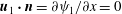
 $\boldsymbol{u}=\boldsymbol{u}_{B}(z,t)\equiv 0$
, and the solution to the thermal diffusion equation (2.6) subject to (2.2a
) and (2.3a
) is
$\boldsymbol{u}=\boldsymbol{u}_{B}(z,t)\equiv 0$
, and the solution to the thermal diffusion equation (2.6) subject to (2.2a
) and (2.3a
) is
 $$\begin{eqnarray}\displaystyle {\it\theta}={\it\theta}_{B}\equiv \text{erf}\left(\frac{z}{2\sqrt{t}}\right)+\text{exp}\left(-\frac{z^{2}}{4t}\right)\text{erfcx}\left(\frac{z}{2\sqrt{t}}+\mathit{Bi}\sqrt{t}\right). & & \displaystyle\end{eqnarray}$$
where the scaled complementary error function is defined by
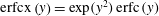 $\text{erfcx}\left(y\right)=\text{exp}(y^{2})\,\text{erfc}\,(y)$
(see Carslaw & Jaeger Reference Carslaw and Jaeger1959). The
$\text{erfcx}\left(y\right)=\text{exp}(y^{2})\,\text{erfc}\,(y)$
(see Carslaw & Jaeger Reference Carslaw and Jaeger1959). The
 $z$
-dependence contains two effective length scales that evolve over time, the thermal diffusion length scale,
$z$
-dependence contains two effective length scales that evolve over time, the thermal diffusion length scale,
 $\sqrt{t}$
in dimensionless scaling, and a length scale associated with the radiative cooling effects,
$\sqrt{t}$
in dimensionless scaling, and a length scale associated with the radiative cooling effects,
 $1/\mathit{Bi}$
.
$1/\mathit{Bi}$
.
For
 $z+2\mathit{Bi}\,t\gg 2\sqrt{t}$
, the solution reduces to
$z+2\mathit{Bi}\,t\gg 2\sqrt{t}$
, the solution reduces to
 $$\begin{eqnarray}\displaystyle {\it\theta}_{B}\sim \text{erf}\left(\frac{z}{2\sqrt{t}}\right),\quad \text{for}~\frac{z+2\mathit{Bi}\,t}{2\sqrt{t}}\gg 1. & & \displaystyle\end{eqnarray}$$
We refer to (2.10) as the conductive limit because it arises when
 $\mathit{Bi}\rightarrow \infty$
, but note that it also applies for finite
$\mathit{Bi}\rightarrow \infty$
, but note that it also applies for finite
 $\mathit{Bi}$
at large depths with
$\mathit{Bi}$
at large depths with
 $z\gg \sqrt{t}$
, or long times with
$z\gg \sqrt{t}$
, or long times with
 $t\gg 1/\mathit{Bi}^{2}$
.
$t\gg 1/\mathit{Bi}^{2}$
.
3 Stability analysis
To perform a stability analysis on this base state, we consider general perturbations,
 ${\it\theta}_{1}$
and
${\it\theta}_{1}$
and
 ${\it\psi}_{1}$
, satisfying
${\it\psi}_{1}$
, satisfying
 $$\begin{eqnarray}\displaystyle {\it\theta}(x,z,t)={\it\theta}_{B}(z,t)+{\it\theta}_{1}(x,z,t),\quad {\it\psi}(x,z,t)={\it\psi}_{1}(x,z,t), & & \displaystyle\end{eqnarray}$$
with
 $\boldsymbol{u}_{1}=\boldsymbol{{\rm\nabla}}\times {\it\psi}_{1}\boldsymbol{e}_{\boldsymbol{y}}$
. We use the energy stability method of Slim & Ramakrishnan (Reference Slim and Ramakrishnan2010) to calculate the stability of the system by considering the maximal growth rate of arbitrarily sized perturbations. The method therefore provides a strong lower bound for the stability of the system, with all disturbances decaying below the threshold it provides, and convection permitted above it. For perfectly conducting boundaries, a number of methods have been used to determine the onset of instability, but we note that the these other methods generally assume small linear perturbations which means they may not capture an instability triggered by a finite amplitude perturbation. The popular propagation method (e.g. Kim & Choi Reference Kim and Choi2012) also requires that perturbations spread vertically with the growing thermal diffusion length scale, which may break down here following the introduction of a second length scale,
$\boldsymbol{u}_{1}=\boldsymbol{{\rm\nabla}}\times {\it\psi}_{1}\boldsymbol{e}_{\boldsymbol{y}}$
. We use the energy stability method of Slim & Ramakrishnan (Reference Slim and Ramakrishnan2010) to calculate the stability of the system by considering the maximal growth rate of arbitrarily sized perturbations. The method therefore provides a strong lower bound for the stability of the system, with all disturbances decaying below the threshold it provides, and convection permitted above it. For perfectly conducting boundaries, a number of methods have been used to determine the onset of instability, but we note that the these other methods generally assume small linear perturbations which means they may not capture an instability triggered by a finite amplitude perturbation. The popular propagation method (e.g. Kim & Choi Reference Kim and Choi2012) also requires that perturbations spread vertically with the growing thermal diffusion length scale, which may break down here following the introduction of a second length scale,
 $\hat{l}_{c}$
, to the infinite-depth problem.
$\hat{l}_{c}$
, to the infinite-depth problem.
However, it is important to remember that the stability bound presented here identifies the first perturbations that are able to grow in amplitude. Determining the time for convective disturbances to develop to a specified finite-amplitude threshold constitutes a different problem, and would depend on both the full details of the initial perturbation and the subsequent time development of these disturbances (see Tilton & Riaz Reference Tilton and Riaz2014; Emami-Meybodi et al. Reference Emami-Meybodi, Hassanzadeh, Green and Ennis-King2015).
When interpreting the results we will also make use of relevant linearised dynamics (discussed in § 3.2) where the perturbations are assumed to be small compared with the base state.
3.1 Energy stability method
Our main calculations follow the energy stability method of Slim & Ramakrishnan (Reference Slim and Ramakrishnan2010), which we summarise below. This method considers the maximal growth rate of the perturbation-amplitude functional:
 $$\begin{eqnarray}\displaystyle E_{0}=\int _{V}\frac{{\it\theta}_{1}^{2}}{2}\,\text{d}^{3}\boldsymbol{x}. & & \displaystyle\end{eqnarray}$$
The integration volume,
 $V$
, here is over the full depth of the domain and a suitable width which allows horizontal boundary conditions to cancel, as discussed below. By finding the maximal growth rate of this functional with respect to all possible perturbations
$V$
, here is over the full depth of the domain and a suitable width which allows horizontal boundary conditions to cancel, as discussed below. By finding the maximal growth rate of this functional with respect to all possible perturbations
 ${\it\theta}_{1}$
that are constrained by the dynamics in (2.6) and (2.8), we can determine the nonlinear stability of the system with respect to an arbitrary perturbation. We have chosen a functional of
${\it\theta}_{1}$
that are constrained by the dynamics in (2.6) and (2.8), we can determine the nonlinear stability of the system with respect to an arbitrary perturbation. We have chosen a functional of
 ${\it\theta}_{1}$
rather than a functional of
${\it\theta}_{1}$
rather than a functional of
 ${\it\psi}_{1}$
because the equations include no time derivatives of
${\it\psi}_{1}$
because the equations include no time derivatives of
 ${\it\psi}_{1}$
. This functional represents a generalised energy, rather than a physical energy. Differentiating
${\it\psi}_{1}$
. This functional represents a generalised energy, rather than a physical energy. Differentiating
 $E_{0}$
with respect to time and using the energy equation (2.6) to eliminate
$E_{0}$
with respect to time and using the energy equation (2.6) to eliminate
 $\partial {\it\theta}_{1}/\partial t$
leads to
$\partial {\it\theta}_{1}/\partial t$
leads to
 $$\begin{eqnarray}\displaystyle {\dot{E}}_{0}=\frac{\text{d}E_{0}}{\text{d}t}=\int _{V}{\it\theta}_{1}{\rm\nabla}^{2}{\it\theta}_{1}-{\it\theta}_{1}(\boldsymbol{u}_{1}\boldsymbol{\cdot }\boldsymbol{{\rm\nabla}}){\it\theta}_{B}-(\boldsymbol{u}_{1}\boldsymbol{\cdot }\boldsymbol{{\rm\nabla}})\left(\frac{{\it\theta}_{1}^{2}}{2}\right)\,\text{d}^{3}\boldsymbol{x}. & & \displaystyle\end{eqnarray}$$
The nonlinear term in (2.6) gives rise to the non-quadratic third term above. Integrating this term by parts gives
 $$\begin{eqnarray}\displaystyle \int _{V}\boldsymbol{u}_{1}\boldsymbol{\cdot }\boldsymbol{{\rm\nabla}}\left(\frac{{\it\theta}_{1}^{2}}{2}\right)\text{d}^{3}\boldsymbol{x}=\oint _{S}\boldsymbol{n}\boldsymbol{\cdot }\left[\frac{{\it\theta}_{1}^{2}}{2}\boldsymbol{u}_{1}\right]\text{d}^{2}\boldsymbol{x}-\int _{V}\frac{{\it\theta}_{1}^{2}}{2}\boldsymbol{{\rm\nabla}}\boldsymbol{\cdot }\boldsymbol{u}_{1}\,\text{d}^{3}\boldsymbol{x}, & & \displaystyle\end{eqnarray}$$
where
 $S$
is the surface bounding the volume
$S$
is the surface bounding the volume
 $V$
. Incompressibility (2.7b
) causes the contribution from the final term to vanish. We focus on systems where the boundary terms also vanish or are negligible, with
$V$
. Incompressibility (2.7b
) causes the contribution from the final term to vanish. We focus on systems where the boundary terms also vanish or are negligible, with
 $\boldsymbol{u}_{1}\boldsymbol{\cdot }\boldsymbol{n}=\partial {\it\psi}_{1}/\partial x=0$
at
$\boldsymbol{u}_{1}\boldsymbol{\cdot }\boldsymbol{n}=\partial {\it\psi}_{1}/\partial x=0$
at
 $z=0$
and as
$z=0$
and as
 $z\rightarrow \infty$
, and then either assuming horizontal periodicity, impermeable or isothermal sidewalls, or a domain of sufficient width for end contributions to be small compared with the full volume integral. Hence, the only nonlinear term in the original dynamical equations makes no contribution to the stability of the system and we will obtain the same stability results for linearised and nonlinear perturbations.
$z\rightarrow \infty$
, and then either assuming horizontal periodicity, impermeable or isothermal sidewalls, or a domain of sufficient width for end contributions to be small compared with the full volume integral. Hence, the only nonlinear term in the original dynamical equations makes no contribution to the stability of the system and we will obtain the same stability results for linearised and nonlinear perturbations.
We now write the growth rate functional as
 $$\begin{eqnarray}\displaystyle {\it\sigma}=\frac{{\dot{E}}_{0}+{\dot{E}}_{1}}{2E_{0}}, & & \displaystyle\end{eqnarray}$$
where
 ${\dot{E}}_{0}/E_{0}$
is the normalised perturbation growth rate and a new term,
${\dot{E}}_{0}/E_{0}$
is the normalised perturbation growth rate and a new term,
 ${\dot{E}}_{1}/E_{0}$
, is introduced to ensure that any variations on this functional are constrained by the vorticity equation (2.8). We add this constraint using a distributed Lagrange multiplier,
${\dot{E}}_{1}/E_{0}$
, is introduced to ensure that any variations on this functional are constrained by the vorticity equation (2.8). We add this constraint using a distributed Lagrange multiplier,
 ${\it\mu}_{1}(\boldsymbol{x},t)$
, with
${\it\mu}_{1}(\boldsymbol{x},t)$
, with
 $$\begin{eqnarray}\displaystyle {\dot{E}}_{1}=\int _{V}{\it\mu}_{1}\left[{\rm\nabla}^{2}{\it\psi}_{1}+\mathit{Rp}\frac{\partial {\it\theta}_{1}}{\partial x}\right]\,\text{d}^{3}\boldsymbol{x}. & & \displaystyle\end{eqnarray}$$
To find the maximal growth rate
 ${\it\sigma}_{\mathit{max}}$
, we vary
${\it\sigma}_{\mathit{max}}$
, we vary
 ${\it\sigma}$
with respect to
${\it\sigma}$
with respect to
 ${\it\theta}_{1}$
,
${\it\theta}_{1}$
,
 ${\it\psi}_{1}$
and
${\it\psi}_{1}$
and
 ${\it\mu}_{1}$
resulting in the system:
${\it\mu}_{1}$
resulting in the system:
 $$\begin{eqnarray}\displaystyle {\rm\nabla}^{2}{\it\theta}_{1}-\frac{1}{2}\frac{\partial {\it\theta}_{B}}{\partial z}\frac{\partial {\it\psi}_{1}}{\partial x}-{\it\sigma}_{\mathit{max}}{\it\theta}_{1}=\frac{\mathit{Rp}}{2}\frac{\partial {\it\mu}_{1}}{\partial x},\quad {\rm\nabla}^{2}{\it\psi}_{1}=-\mathit{Rp}\frac{\partial {\it\theta}_{1}}{\partial x},\quad {\rm\nabla}^{2}{\it\mu}_{1}+\frac{\partial {\it\theta}_{B}}{\partial z}\frac{\partial {\it\theta}_{1}}{\partial x}=0, & & \displaystyle \nonumber\\ \displaystyle & & \displaystyle\end{eqnarray}$$
with boundary conditions on
 ${\it\mu}_{1}$
identical to those on
${\it\mu}_{1}$
identical to those on
 ${\it\psi}_{1}$
.
${\it\psi}_{1}$
.
Despite considering non-linear perturbations, the resulting derived system (3.7) is linear and invariant under horizontal translations, and so we assume a horizontally periodic perturbation structure and perform a Fourier decomposition with wavenumber,
 $k$
, writing
$k$
, writing
 $$\begin{eqnarray}\displaystyle \left[\begin{array}{@{}c@{}}{\it\theta}_{1}(x,z,t)\\ {\it\psi}_{1}(x,z,t)\\ {\it\mu}_{1}(x,z,t)\end{array}\right]=\left[\begin{array}{@{}c@{}}{\it\theta}_{f}(k,z,t)\\ \text{i}k\,{\it\psi}_{f}(k,z,t)\\ \text{i}k\,{\it\mu}_{f}(k,z,t)\end{array}\right]\text{e}^{\text{i}kx}, & & \displaystyle\end{eqnarray}$$
where the subscript
 $_{f}$
indicates that the variables have been Fourier transformed in the horizontal direction. The eigenvalue problem (3.7) reduces to:
$_{f}$
indicates that the variables have been Fourier transformed in the horizontal direction. The eigenvalue problem (3.7) reduces to:
 $$\begin{eqnarray}\displaystyle \unicode[STIX]{x1D63C}\boldsymbol{y}-\mathit{Rp}\,\unicode[STIX]{x1D63D}\boldsymbol{y}={\it\sigma}_{\mathit{max}}\unicode[STIX]{x1D63E}\boldsymbol{y}, & & \displaystyle\end{eqnarray}$$
 $$\begin{eqnarray}\displaystyle \boldsymbol{y}=\left[\begin{array}{@{}c@{}}{\it\theta}_{f}\\ {\it\psi}_{f}\\ {\it\mu}_{f}\end{array}\right],\quad \unicode[STIX]{x1D63C}=\left[\begin{array}{@{}ccc@{}}\displaystyle \frac{\partial ^{2}}{\partial z^{2}}-k^{2} & \displaystyle \frac{k^{2}}{2}\displaystyle \frac{\partial {\it\theta}_{B}}{\partial z} & 0\\ 0 & \displaystyle \frac{\partial ^{2}}{\partial z^{2}}-k^{2} & 0\\ \displaystyle \frac{\partial {\it\theta}_{B}}{\partial z} & 0 & \displaystyle \frac{\partial ^{2}}{\partial z^{2}}-k^{2}\end{array}\right], & & \displaystyle\end{eqnarray}$$
 $$\begin{eqnarray}\displaystyle \unicode[STIX]{x1D63D}=\left[\begin{array}{@{}ccc@{}}0 & 0 & \displaystyle -\frac{k^{2}}{2}\\ -1 & 0 & 0\\ 0 & 0 & 0\end{array}\right],\quad \unicode[STIX]{x1D63E}=\left[\begin{array}{@{}ccc@{}}1 & 0 & 0\\ 0 & 0 & 0\\ 0 & 0 & 0\end{array}\right]. & & \displaystyle\end{eqnarray}$$
The boundary conditions are expanded in the same way as the dynamical equations and become
 $$\begin{eqnarray}\displaystyle \frac{\partial {\it\theta}_{f}}{\partial z}=\mathit{Bi}\,{\it\theta}_{f},\quad {\it\psi}_{f}=0,\quad {\it\mu}_{f}=0,\quad \text{at}~z=0 & & \displaystyle\end{eqnarray}$$
 $$\begin{eqnarray}\displaystyle {\it\theta}_{f}\rightarrow 0,\quad {\it\psi}_{f}\rightarrow 0,\quad {\it\mu}_{f}\rightarrow 0,\quad \text{as}~z\rightarrow \infty . & & \displaystyle\end{eqnarray}$$
As a final step, we note that time now only appears explicitly through the
 ${\it\theta}_{B}$
terms and can be removed by transforming to the self-similar coordinates natural to the thermal diffusion problem:
${\it\theta}_{B}$
terms and can be removed by transforming to the self-similar coordinates natural to the thermal diffusion problem:
 $$\begin{eqnarray}\displaystyle \tilde{z}=\frac{z}{\sqrt{t}},\quad \tilde{k}=k\sqrt{t},\quad \tilde{\mathit{Rp}}=\mathit{Rp}\sqrt{t},\quad \tilde{\mathit{Bi}}=\mathit{Bi}\sqrt{t},\quad \tilde{{\it\sigma}}={\it\sigma}_{\mathit{max}}t. & & \displaystyle\end{eqnarray}$$
This transformation effectively replaces the non-dimensionalisation length
 $\hat{d}$
with the thermal diffusion length scale
$\hat{d}$
with the thermal diffusion length scale
 $\sqrt{{\it\kappa}\hat{t}}$
and leaves the form of (3.9) and (3.10) unchanged (with each variable replaced by its rescaled counterpart). With the similarity transformation, the base-state temperature profile (2.9) becomes
$\sqrt{{\it\kappa}\hat{t}}$
and leaves the form of (3.9) and (3.10) unchanged (with each variable replaced by its rescaled counterpart). With the similarity transformation, the base-state temperature profile (2.9) becomes
 $$\begin{eqnarray}\displaystyle {\it\theta}_{B}=\text{erf}\left(\frac{\tilde{z}}{2}\right)+\text{exp}\left(-\frac{\tilde{z}^{2}}{4}\right)\text{erfcx}\left(\frac{\tilde{z}}{2}+\tilde{\mathit{Bi}}\right). & & \displaystyle\end{eqnarray}$$
The removal of
 $t$
via this rescaling has the advantage of reducing the parameter space that needs to be considered when constraining the stability and we calculate our results in these similarity coordinates, corresponding to scales measured relative to the instantaneous thickness of the thermal boundary layer, before later translating back to time-independent physical scales. Note also that by performing this transformation after deriving the stability system (3.9) we have avoided any a priori assumption of self-similar disturbances, so that our energy stability analysis encompasses general two-dimensional disturbances rather than just disturbances confined to spread at the same rate as the boundary layer.
$t$
via this rescaling has the advantage of reducing the parameter space that needs to be considered when constraining the stability and we calculate our results in these similarity coordinates, corresponding to scales measured relative to the instantaneous thickness of the thermal boundary layer, before later translating back to time-independent physical scales. Note also that by performing this transformation after deriving the stability system (3.9) we have avoided any a priori assumption of self-similar disturbances, so that our energy stability analysis encompasses general two-dimensional disturbances rather than just disturbances confined to spread at the same rate as the boundary layer.
This eigenvalue problem can be solved for the maximal growth rate at a given Rayleigh number, wavenumber and Biot number, with instability allowed if the real part of
 $\tilde{{\it\sigma}}$
is greater than zero. This yields the neutral stability curve
$\tilde{{\it\sigma}}$
is greater than zero. This yields the neutral stability curve
 $\tilde{\mathit{Rp}}(\tilde{k},\tilde{\mathit{Bi}})$
where the real part of the growth rate is equal to zero. If the imaginary part of
$\tilde{\mathit{Rp}}(\tilde{k},\tilde{\mathit{Bi}})$
where the real part of the growth rate is equal to zero. If the imaginary part of
 $\tilde{{\it\sigma}}$
is also zero on the neutral stability curve, then the neutral stability curve can be found directly by setting
$\tilde{{\it\sigma}}$
is also zero on the neutral stability curve, then the neutral stability curve can be found directly by setting
 $\tilde{{\it\sigma}}=0$
in (3.9) and solving for
$\tilde{{\it\sigma}}=0$
in (3.9) and solving for
 $\tilde{\mathit{Rp}}$
. Whilst we did not formally prove that the growth rate is purely real, we found in preliminary investigations that there were no complex growth rates for a sample of Biot numbers,
$\tilde{\mathit{Rp}}$
. Whilst we did not formally prove that the growth rate is purely real, we found in preliminary investigations that there were no complex growth rates for a sample of Biot numbers,
 $\tilde{\mathit{Bi}}=0.05$
, 1, 50, as well as when
$\tilde{\mathit{Bi}}=0.05$
, 1, 50, as well as when
 $\tilde{\mathit{Bi}}\rightarrow \infty$
, and that both of methods produced the same results for the position of the neutral stability curve. To accelerate the computations, we therefore neglect oscillatory modes and set the growth rate to zero in all subsequent calculations and solve for the neutral stability curve directly.
$\tilde{\mathit{Bi}}\rightarrow \infty$
, and that both of methods produced the same results for the position of the neutral stability curve. To accelerate the computations, we therefore neglect oscillatory modes and set the growth rate to zero in all subsequent calculations and solve for the neutral stability curve directly.
3.2 Linearised dynamics
Having established above that the energy stability method yields the same stability criteria for linear and nonlinear perturbations, we will also make use of linearised dynamics when interpreting our results. We assume that the perturbations in equation (3.1) are small compared with the base-state values, and terms that are quadratic in perturbations can be neglected. The linearised forms of (2.6) and (2.8) are
 $$\begin{eqnarray}\displaystyle \frac{\partial {\it\theta}_{1}}{\partial t}+\frac{\partial {\it\theta}_{B}}{\partial z}\frac{\partial {\it\psi}_{1}}{\partial x}={\rm\nabla}^{2}{\it\theta}_{1},\quad {\rm\nabla}^{2}{\it\psi}_{1}=-\mathit{Rp}\,\frac{\partial {\it\theta}_{1}}{\partial x}. & & \displaystyle\end{eqnarray}$$
Eliminating
 ${\it\theta}_{1}$
results in
${\it\theta}_{1}$
results in
 $$\begin{eqnarray}\displaystyle \left(\frac{\partial }{\partial t}-{\rm\nabla}^{2}\right){\rm\nabla}^{2}{\it\psi}_{1}=\mathit{Rp}\,\frac{\partial {\it\theta}_{B}}{\partial z}\,\frac{\partial ^{2}{\it\psi}_{1}}{\partial x^{2}}. & & \displaystyle\end{eqnarray}$$
Thus, the linearised perturbation dynamics are driven by the quantity
 $\mathit{Rp}\,\partial {\it\theta}_{B}/\partial z$
. We will make use of this observation later when interpreting results, noting that the form of this equation is unchanged under the similarity transformation (3.11).
$\mathit{Rp}\,\partial {\it\theta}_{B}/\partial z$
. We will make use of this observation later when interpreting results, noting that the form of this equation is unchanged under the similarity transformation (3.11).
4 Numerical method
To solve the eigenvalue problem in (3.9), we use a Chebyshev pseudospectral discretisation of the three variables,
 ${\it\theta}_{f}$
,
${\it\theta}_{f}$
,
 ${\it\psi}_{f}$
and
${\it\psi}_{f}$
and
 ${\it\mu}_{f}$
, and the differential operators are rewritten as matrix operators on the Chebyshev modes (see Trefethen Reference Trefethen2000). The discretised form of the boundary conditions (3.10) are algebraically rearranged to express the boundary values in terms of the internal values. This is then used to write an eigenvalue problem for the internal points with eigenfunctions that satisfy both the dynamical equations and boundary conditions.
${\it\mu}_{f}$
, and the differential operators are rewritten as matrix operators on the Chebyshev modes (see Trefethen Reference Trefethen2000). The discretised form of the boundary conditions (3.10) are algebraically rearranged to express the boundary values in terms of the internal values. This is then used to write an eigenvalue problem for the internal points with eigenfunctions that satisfy both the dynamical equations and boundary conditions.
Convergence testing was performed to ensure that the results are numerically consistent, and independent of both the number of Chebyshev modes used,
 $N_{z}$
, and the numerically imposed finite domain depth,
$N_{z}$
, and the numerically imposed finite domain depth,
 $\tilde{H}$
, for suitably large
$\tilde{H}$
, for suitably large
 $\tilde{H}$
. The resolution was increased at fixed
$\tilde{H}$
. The resolution was increased at fixed
 $\tilde{H}$
to obtain numerical convergence. This was then repeated at larger
$\tilde{H}$
to obtain numerical convergence. This was then repeated at larger
 $\tilde{H}$
until the resolution-converged values also showed no significant variation with depth. For
$\tilde{H}$
until the resolution-converged values also showed no significant variation with depth. For
 $\tilde{\mathit{Bi}}>1$
, good convergence is found using
$\tilde{\mathit{Bi}}>1$
, good convergence is found using
 $N_{z}\geqslant 40$
and
$N_{z}\geqslant 40$
and
 $\tilde{H}\geqslant 70$
. For
$\tilde{H}\geqslant 70$
. For
 $\tilde{\mathit{Bi}}<1$
, a deeper domain and more grid points were needed. For
$\tilde{\mathit{Bi}}<1$
, a deeper domain and more grid points were needed. For
 $\tilde{\mathit{Bi}}=0.001$
, the lowest Biot number investigated, convergence was only found once
$\tilde{\mathit{Bi}}=0.001$
, the lowest Biot number investigated, convergence was only found once
 $N_{z}\geqslant 90$
and
$N_{z}\geqslant 90$
and
 $\tilde{H}\geqslant 475$
.
$\tilde{H}\geqslant 475$
.
5 Results
To test the accuracy of our code, we first solved the porous boundary layer convection problem in the limit of a perfectly conducting boundary, with an infinite Biot number. We found the critical wavenumber,
 $\tilde{k}_{\infty }$
, and Rayleigh number,
$\tilde{k}_{\infty }$
, and Rayleigh number,
 $\tilde{\mathit{Rp}}_{\infty }$
, to be
$\tilde{\mathit{Rp}}_{\infty }$
, to be
 $$\begin{eqnarray}\displaystyle \tilde{k}_{\infty }=0.378,\quad \tilde{\mathit{Rp}}_{\infty }=6.92, & & \displaystyle\end{eqnarray}$$
in agreement with the results of Slim & Ramakrishnan (Reference Slim and Ramakrishnan2010), who used an equivalent definition of stability. The results here are also of a similar magnitude to calculations using alternative definitions of stability (see Tilton et al.
Reference Tilton, Daniel and Riaz2013 for a review). We note that the fixed dimensionless wavenumber
 $\tilde{k}_{\infty }$
and Rayleigh number
$\tilde{k}_{\infty }$
and Rayleigh number
 $\tilde{\mathit{Rp}}_{\infty }$
results from the similarity transformation (3.11), and leads to time dependence in physical coordinates. Reversing the transformation leads to a dynamic stability criteria compared with the fixed physical scales.
$\tilde{\mathit{Rp}}_{\infty }$
results from the similarity transformation (3.11), and leads to time dependence in physical coordinates. Reversing the transformation leads to a dynamic stability criteria compared with the fixed physical scales.
The Biot number appears in the upper boundary conditions (2.2a
) and in the base-state temperature profile (3.12). In addition to the full system calculations, we ran two additional sets of diagnostic simulations as sensitivity studies to isolate the impacts of
 $\tilde{\mathit{Bi}}$
-dependent changes of potential energy in the background profile, and
$\tilde{\mathit{Bi}}$
-dependent changes of potential energy in the background profile, and
 $\tilde{\mathit{Bi}}$
-dependent modulation of the perturbation boundary conditions. The profile effects set, denoted by superscript
$\tilde{\mathit{Bi}}$
-dependent modulation of the perturbation boundary conditions. The profile effects set, denoted by superscript
 $^{p}$
, uses a conductive boundary condition,
$^{p}$
, uses a conductive boundary condition,
 ${\it\theta}_{f}=0$
at
${\it\theta}_{f}=0$
at
 $z=0$
, for the perturbation but the full
$z=0$
, for the perturbation but the full
 $\tilde{\mathit{Bi}}$
-dependent base-state temperature profile (3.12). Meanwhile the boundary effects set, denoted by superscript
$\tilde{\mathit{Bi}}$
-dependent base-state temperature profile (3.12). Meanwhile the boundary effects set, denoted by superscript
 $^{b}$
, uses the conductive limit of the base-state temperature profile,
$^{b}$
, uses the conductive limit of the base-state temperature profile,
 ${\it\theta}_{B}\sim \text{erf}\left(\tilde{z}/2\right)$
, but maintaining the full
${\it\theta}_{B}\sim \text{erf}\left(\tilde{z}/2\right)$
, but maintaining the full
 $\tilde{\mathit{Bi}}$
-dependent boundary condition for the perturbation. These two extra sets are not intended to represent physically realisable configurations, but instead provide diagnostic insight into the mathematical scalings obtained.
$\tilde{\mathit{Bi}}$
-dependent boundary condition for the perturbation. These two extra sets are not intended to represent physically realisable configurations, but instead provide diagnostic insight into the mathematical scalings obtained.
Figure 2(a) shows how the Rayleigh number at neutral stability, with
 $\tilde{{\it\sigma}}=0$
, varies with wavenumber,
$\tilde{{\it\sigma}}=0$
, varies with wavenumber,
 $\tilde{k}$
, and Biot number,
$\tilde{k}$
, and Biot number,
 $\tilde{\mathit{Bi}}$
, along with showing the critical wavenumbers,
$\tilde{\mathit{Bi}}$
, along with showing the critical wavenumbers,
 $\tilde{k}_{c}$
. Figure 2(b) shows the variation of the resulting critical Rayleigh numbers,
$\tilde{k}_{c}$
. Figure 2(b) shows the variation of the resulting critical Rayleigh numbers,
 $\tilde{\mathit{Rp}}_{c}$
, with
$\tilde{\mathit{Rp}}_{c}$
, with
 $\tilde{\mathit{Bi}}$
. It is clear that decreasing the Biot number monotonically increases the critical Rayleigh number for the full system (figure 2
b), while the effect on the critical wave number is more complex. There is an increase when compared with the conductive limit for
$\tilde{\mathit{Bi}}$
. It is clear that decreasing the Biot number monotonically increases the critical Rayleigh number for the full system (figure 2
b), while the effect on the critical wave number is more complex. There is an increase when compared with the conductive limit for
 $\tilde{\mathit{Bi}}>O(1)$
and a decrease for
$\tilde{\mathit{Bi}}>O(1)$
and a decrease for
 $\tilde{\mathit{Bi}}<O(1)$
, as shown in figure 2(a). There are two distinct regimes for large and small Biot numbers, which are emphasised using a change of scale at
$\tilde{\mathit{Bi}}<O(1)$
, as shown in figure 2(a). There are two distinct regimes for large and small Biot numbers, which are emphasised using a change of scale at
 $\tilde{k}=0.3$
in figure 2(a) and
$\tilde{k}=0.3$
in figure 2(a) and
 $\tilde{\mathit{Rp}}_{c}=12.5$
in figure 2(b). We find no indication of any secondary minima in the stability curves,
$\tilde{\mathit{Rp}}_{c}=12.5$
in figure 2(b). We find no indication of any secondary minima in the stability curves,
 $\tilde{\mathit{Rp}}_{c}(\tilde{k})$
, for each
$\tilde{\mathit{Rp}}_{c}(\tilde{k})$
, for each
 $\tilde{\mathit{Bi}}$
.
$\tilde{\mathit{Bi}}$
.

Figure 2. Stability properties against Biot number. (a) The colour scale shows the Rayleigh number at neutral stability as a function of wavenumber and Biot number. Overlayed are the critical wavenumbers of the three calculation sets described in the text. To aid viewing of the different limits, the wavenumber is displayed on a logarithmic scale for
 $\tilde{k}<0.3$
and linear scale for
$\tilde{k}<0.3$
and linear scale for
 $\tilde{k}>0.3$
, with the transition marked by a dashed line. (b) The critical Rayleigh number varies with Biot number. The data is shown on a linear scale for
$\tilde{k}>0.3$
, with the transition marked by a dashed line. (b) The critical Rayleigh number varies with Biot number. The data is shown on a linear scale for
 $\tilde{\mathit{Rp}}_{c}<12.5$
and a logarithmic scale for
$\tilde{\mathit{Rp}}_{c}<12.5$
and a logarithmic scale for
 $\tilde{\mathit{Rp}}_{c}>12.5$
.
$\tilde{\mathit{Rp}}_{c}>12.5$
.
The structure of the instability differs in these two limits, as illustrated in figure 3. For large Biot numbers, the unstable convective cells are narrower and do not penetrate as deeply as the cells for low Biot numbers. By normalising the perturbations such that the integrated amplitude over all three perturbation variables is equal to 1, we can also see that the thermal variations and velocities have significantly larger amplitude when the Biot number is large. This suggests that the instability will be more intense in this regime but less disperse. This conclusion is also supported by looking at the growth rates,
 $\tilde{{\it\sigma}}$
, at the critical wavenumber and with a Rayleigh number equal to double the critical value. When
$\tilde{{\it\sigma}}$
, at the critical wavenumber and with a Rayleigh number equal to double the critical value. When
 $\tilde{\mathit{Bi}}=100$
, this non-dimensional growth rate is
$\tilde{\mathit{Bi}}=100$
, this non-dimensional growth rate is
 $\tilde{{\it\sigma}}=0.35$
, while for
$\tilde{{\it\sigma}}=0.35$
, while for
 $\tilde{\mathit{Bi}}=0.022$
the growth rate is
$\tilde{\mathit{Bi}}=0.022$
the growth rate is
 $\tilde{{\it\sigma}}=0.016$
, which suggests that after onset of instability, the disturbance will initially develop more rapidly at large Biot numbers than it will for small Biot numbers. However, determining the long-time development will require a study of the time-dependent evolution of perturbations to confirm whether such trends continue.
$\tilde{{\it\sigma}}=0.016$
, which suggests that after onset of instability, the disturbance will initially develop more rapidly at large Biot numbers than it will for small Biot numbers. However, determining the long-time development will require a study of the time-dependent evolution of perturbations to confirm whether such trends continue.

Figure 3. Representative convective instability structure for (a)
 $\tilde{B}i=100$
, and (b)
$\tilde{B}i=100$
, and (b)
 $\tilde{B}i=0.022$
. The colour scale shows the thermal variation with hot regions coloured red and cold regions coloured blue. Stream lines are also shown with clockwise cells in black and anticlockwise cells in grey, with
$\tilde{B}i=0.022$
. The colour scale shows the thermal variation with hot regions coloured red and cold regions coloured blue. Stream lines are also shown with clockwise cells in black and anticlockwise cells in grey, with
 ${\it\psi}_{f}=\pm 0.03$
,
${\it\psi}_{f}=\pm 0.03$
,
 $\pm 0.06$
and
$\pm 0.06$
and
 $\pm 0.09$
contours plotted. Note that the temperature scale for (a) is 100 times larger than the scale in (b) and there is no
$\pm 0.09$
contours plotted. Note that the temperature scale for (a) is 100 times larger than the scale in (b) and there is no
 ${\it\psi}_{f}=0.09$
contour in (b). The same vertical and horizontal scales are used in the two panels and the instability continues periodically beyond the region shown, with alternating directions of neighbouring convection cells.
${\it\psi}_{f}=0.09$
contour in (b). The same vertical and horizontal scales are used in the two panels and the instability continues periodically beyond the region shown, with alternating directions of neighbouring convection cells.
5.1 High Biot number limit
Boundaries that can rapidly remove heat from a medium have a large Biot number and behave as good effective conductors, with an infinite Biot number representing a perfectly conducting boundary. Behaviour in the large Biot number limit,
 $\tilde{\mathit{Bi}}\gg 1$
, is dominated by the limiting case of a perfectly conducting boundary (discussed above) with only small
$\tilde{\mathit{Bi}}\gg 1$
, is dominated by the limiting case of a perfectly conducting boundary (discussed above) with only small
 $\tilde{\mathit{Bi}}$
-dependent variations. To illustrate the underlying scalings, figure 4 shows compensated plots taking the deviation from the perfectly conducting limit and scaling by the Biot number, plotting
$\tilde{\mathit{Bi}}$
-dependent variations. To illustrate the underlying scalings, figure 4 shows compensated plots taking the deviation from the perfectly conducting limit and scaling by the Biot number, plotting
 $\tilde{\mathit{Bi}}(\tilde{\mathit{Rp}}_{c}-\tilde{\mathit{Rp}}_{\infty })$
for the compensated critical Rayleigh number and
$\tilde{\mathit{Bi}}(\tilde{\mathit{Rp}}_{c}-\tilde{\mathit{Rp}}_{\infty })$
for the compensated critical Rayleigh number and
 $\tilde{\mathit{Bi}}(\tilde{k}_{c}-\tilde{k}_{\infty })$
for the compensated critical wavenumber. We observe that both groupings tend to a constant value for large Biot numbers. The critical Rayleigh number and critical wavenumber therefore behave as
$\tilde{\mathit{Bi}}(\tilde{k}_{c}-\tilde{k}_{\infty })$
for the compensated critical wavenumber. We observe that both groupings tend to a constant value for large Biot numbers. The critical Rayleigh number and critical wavenumber therefore behave as
 $$\begin{eqnarray}\displaystyle & \displaystyle \tilde{\mathit{Rp}}_{c}\sim \tilde{\mathit{Rp}}_{\infty }+\frac{3.25}{\tilde{\mathit{Bi}}},\quad \tilde{\mathit{Rp}}_{c}^{p}\sim \tilde{\mathit{Rp}}_{\infty }+\frac{6.35}{\tilde{\mathit{Bi}}},\quad \tilde{\mathit{Rp}}_{c}^{b}\sim \tilde{\mathit{Rp}}_{\infty }-\frac{3.10}{\tilde{\mathit{Bi}}},\quad \text{for}~\tilde{\mathit{Bi}}\gg 1, & \displaystyle \nonumber\\ \displaystyle & & \displaystyle\end{eqnarray}$$
 $$\begin{eqnarray}\displaystyle & \displaystyle \tilde{k}_{c}\sim \tilde{k}_{\infty }+\frac{0.054}{\tilde{\mathit{Bi}}},\quad \tilde{k}_{c}^{p}\sim \tilde{k}_{\infty }+\frac{0.088}{\tilde{\mathit{Bi}}},\quad \tilde{k}_{c}^{b}\sim \tilde{k}_{\infty }-\frac{0.034}{\tilde{\mathit{Bi}}},\quad \text{for}~\tilde{\mathit{Bi}}\gg 1, & \displaystyle \nonumber\\ \displaystyle & & \displaystyle\end{eqnarray}$$
corresponding to the full calculation, profile effects and boundary effects in each of (5.2) and (5.3). These trends remain accurate for
 $\tilde{\mathit{Bi}}\gtrsim 5$
. We also note that in both cases the sum of the deviations caused by the profile effects only, plus the deviations caused by the boundary effects only is very similar to the deviation of the full system
$\tilde{\mathit{Bi}}\gtrsim 5$
. We also note that in both cases the sum of the deviations caused by the profile effects only, plus the deviations caused by the boundary effects only is very similar to the deviation of the full system
 $$\begin{eqnarray}\displaystyle {\rm\Delta}\tilde{\mathit{Rp}}_{c}=\tilde{\mathit{Rp}}_{c}-\tilde{\mathit{Rp}}_{\infty }\approx {\rm\Delta}\tilde{\mathit{Rp}}_{c}^{p}+{\rm\Delta}\tilde{\mathit{Rp}}_{c}^{b},\quad {\rm\Delta}\tilde{k}_{c}=\tilde{k}_{c}-\tilde{k}_{\infty }\approx {\rm\Delta}\tilde{k}_{c}^{p}+{\rm\Delta}\tilde{k}_{c}^{b}. & & \displaystyle\end{eqnarray}$$
This suggests that nonlinear interactions between the changes in the base-state profile and perturbation boundary condition are negligible when the Biot number is large.

Figure 4. Scaled deviations from the perfectly conducting limit: (a)
 $\tilde{\mathit{Bi}}(\tilde{\mathit{Rp}}_{c}-\tilde{\mathit{Rp}}_{\infty })$
for the compensated critical Rayleigh number and (b)
$\tilde{\mathit{Bi}}(\tilde{\mathit{Rp}}_{c}-\tilde{\mathit{Rp}}_{\infty })$
for the compensated critical Rayleigh number and (b)
 $\tilde{\mathit{Bi}}(\tilde{k}_{c}-\tilde{k}_{\infty })$
for the compensated critical wavenumber. The scaled deviation of both the Rayleigh number and wavenumber asymptote to a constant value for large Biot numbers. In this limit, the deviation for the full system matches a linear sum of the deviation caused by the boundary effects, and the deviation caused by profile effects. At small Biot numbers,
$\tilde{\mathit{Bi}}(\tilde{k}_{c}-\tilde{k}_{\infty })$
for the compensated critical wavenumber. The scaled deviation of both the Rayleigh number and wavenumber asymptote to a constant value for large Biot numbers. In this limit, the deviation for the full system matches a linear sum of the deviation caused by the boundary effects, and the deviation caused by profile effects. At small Biot numbers,
 $\tilde{\mathit{Bi}}(\tilde{\mathit{Rp}}_{c}-\tilde{\mathit{Rp}}_{\infty })$
again tends to a constant (but different) value for the full dynamics and profile effects.
$\tilde{\mathit{Bi}}(\tilde{\mathit{Rp}}_{c}-\tilde{\mathit{Rp}}_{\infty })$
again tends to a constant (but different) value for the full dynamics and profile effects.
The
 $O(1/\tilde{\mathit{Bi}})$
deviations found in this limit can be considered as a first-order expansion in the small parameter
$O(1/\tilde{\mathit{Bi}})$
deviations found in this limit can be considered as a first-order expansion in the small parameter
 $1/\tilde{\mathit{Bi}}$
around the perfectly conducting limit and this is also reflected in the profiles of
$1/\tilde{\mathit{Bi}}$
around the perfectly conducting limit and this is also reflected in the profiles of
 ${\it\theta}_{f}$
,
${\it\theta}_{f}$
,
 ${\it\psi}_{f}$
and
${\it\psi}_{f}$
and
 ${\it\mu}_{f}$
having only small deviations from the conducting limit (not shown here). The observed signs of the deviations are explained as follows. For large Biot numbers, the thermal forcing term identified previously in (3.14) is approximately:
${\it\mu}_{f}$
having only small deviations from the conducting limit (not shown here). The observed signs of the deviations are explained as follows. For large Biot numbers, the thermal forcing term identified previously in (3.14) is approximately:
 $$\begin{eqnarray}\displaystyle \tilde{\mathit{Rp}}\frac{\partial {\it\theta}_{B}}{\partial \tilde{z}}=\frac{\tilde{\mathit{Rp}}}{\sqrt{{\rm\pi}}}\text{exp}\left(-\frac{\tilde{z}^{2}}{4}\right)\left[1-\frac{\tilde{z}}{2\tilde{\mathit{Bi}}}+O\left(\frac{1}{\tilde{\mathit{Bi}}^{2}}\right)\right],\quad \text{for}~\tilde{\mathit{Bi}}\gg 1. & & \displaystyle\end{eqnarray}$$
When the Biot number decreases from the perfectly conducting limit, the thermal forcing decreases because the potential energy available for convection has been reduced. This change in the background profile necessarily causes an increase in the critical Rayleigh number,
 ${\rm\Delta}\tilde{\mathit{Rp}}_{c}^{p}>0$
, but it also affects the critical wavenumber by changing the vertical distribution of the available energy. By decreasing the energy available at depth to a greater extent than the energy available close to the boundary, the change in forcing confines the convection to a shallower layer near the surface. In turn, this is consistent with a smaller convective wavelength and larger wavenumber,
${\rm\Delta}\tilde{\mathit{Rp}}_{c}^{p}>0$
, but it also affects the critical wavenumber by changing the vertical distribution of the available energy. By decreasing the energy available at depth to a greater extent than the energy available close to the boundary, the change in forcing confines the convection to a shallower layer near the surface. In turn, this is consistent with a smaller convective wavelength and larger wavenumber,
 ${\rm\Delta}\tilde{k}_{c}^{p}>0$
, when viewed as relative fractions of the corresponding diffusion length scale of the growing boundary layer.
${\rm\Delta}\tilde{k}_{c}^{p}>0$
, when viewed as relative fractions of the corresponding diffusion length scale of the growing boundary layer.
However, the Biot number dependence of the perturbation boundary condition causes the opposite effect, as shown by the scaling of the boundary effects simulations. The change in boundary condition allows the energy close to the upper boundary to be more effectively utilised by permitting modes to develop with non-zero thermal variation on the upper boundary. This tends to decrease the critical Rayleigh number,
 ${\rm\Delta}\tilde{\mathit{Rp}}_{c}^{b}<0$
. It is also consistent with a tendency for stronger and deeper-penetrating convection, leading to larger convective cells with a longer wavelength and smaller wavenumber,
${\rm\Delta}\tilde{\mathit{Rp}}_{c}^{b}<0$
. It is also consistent with a tendency for stronger and deeper-penetrating convection, leading to larger convective cells with a longer wavelength and smaller wavenumber,
 ${\rm\Delta}\tilde{k}_{c}^{b}<0$
. Barletta et al. (Reference Barletta, Tyvand and Nygård2015) noted a similar effect for steady-state convection in a finite horizontal domain. As the Biot number decreases they observed that the critical Rayleigh number and critical wavenumber also decrease as the boundary conditions become less restrictive on the allowable perturbations (note that their parameters
${\rm\Delta}\tilde{k}_{c}^{b}<0$
. Barletta et al. (Reference Barletta, Tyvand and Nygård2015) noted a similar effect for steady-state convection in a finite horizontal domain. As the Biot number decreases they observed that the critical Rayleigh number and critical wavenumber also decrease as the boundary conditions become less restrictive on the allowable perturbations (note that their parameters
 $a_{i}$
and
$a_{i}$
and
 $b_{i}$
 $(i=1,2)$
are equivalent to
$(i=1,2)$
are equivalent to
 $1/\mathit{Bi}$
).
$1/\mathit{Bi}$
).
The combined effect of these profile and boundary effects is an increase in both the critical Rayleigh number and critical wavenumber compared to the perfectly conducting limit. This suggests that the changes caused by the available potential energy in the background profile are more significant than the modification to the heat-flux boundary conditions on the growing perturbations.
The above results have considered the impact of effective boundary conductivity on wavenumbers and Rayleigh numbers scaled relative to the time-dependent thermal diffusion timescale
 $\sqrt{{\it\kappa}\hat{t}}$
. We can invert the scaling behaviour in (5.2) to find the physical instability time of the system
$\sqrt{{\it\kappa}\hat{t}}$
. We can invert the scaling behaviour in (5.2) to find the physical instability time of the system
 $$\begin{eqnarray}\displaystyle \hat{t}_{i}=47.9\,\hat{t}_{b}[1+0.136\,\text{R}{\rm \small{B}}+O(\text{R}{\rm \small{B}})^{2}],\quad \text{for}~\text{R}{\rm \small{B}}\ll 1, & & \displaystyle\end{eqnarray}$$
where the buoyancy time scale is
 $\hat{t}_{b}=\hat{l}_{b}^{2}/{\it\kappa}$
, and we define the effective boundary Rayleigh number as the ratio of boundary-cooling and buoyancy lengthscales,
$\hat{t}_{b}=\hat{l}_{b}^{2}/{\it\kappa}$
, and we define the effective boundary Rayleigh number as the ratio of boundary-cooling and buoyancy lengthscales,
 $$\begin{eqnarray}\displaystyle \text{R}{\rm \small{B}}=\frac{\mathit{Rp}}{\mathit{ Bi }}=\frac{g{\it\alpha}{\rm\Delta}T{\it\Pi}_{0}{\it\Lambda}{\it\lambda}^{\ast }}{{\it\kappa}{\it\nu}h}=\frac{\hat{l}_{c}}{\hat{l}_{b}}. & & \displaystyle\end{eqnarray}$$
The instability time (5.6) is dominated by the buoyancy time scale
 $\hat{t}_{b}$
. As the heat transfer coefficient increases,
$\hat{t}_{b}$
. As the heat transfer coefficient increases,
 $h\rightarrow \infty$
, the boundary length scale correspondingly decreases,
$h\rightarrow \infty$
, the boundary length scale correspondingly decreases,
 $\hat{l}_{c}\rightarrow 0$
, and the time of instability reduces to the time found by Slim & Ramakrishnan (Reference Slim and Ramakrishnan2010). For finite
$\hat{l}_{c}\rightarrow 0$
, and the time of instability reduces to the time found by Slim & Ramakrishnan (Reference Slim and Ramakrishnan2010). For finite
 $h$
,
$h$
,
 $\hat{l}_{c}$
is non-zero and convective instability is delayed in a way that depends on the boundary Rayleigh number (5.7). Larger values of
$\hat{l}_{c}$
is non-zero and convective instability is delayed in a way that depends on the boundary Rayleigh number (5.7). Larger values of
 $\text{R}{\rm \small{B}}$
correspond to increasingly imperfect cooling and convection is delayed by a greater amount. The conductive limit corresponds to
$\text{R}{\rm \small{B}}$
correspond to increasingly imperfect cooling and convection is delayed by a greater amount. The conductive limit corresponds to
 $\text{R}{\rm \small{B}}\rightarrow 0$
, and the subsequent expansion (5.6) in small
$\text{R}{\rm \small{B}}\rightarrow 0$
, and the subsequent expansion (5.6) in small
 $\text{R}{\rm \small{B}}$
is accurate to within 10 % for
$\text{R}{\rm \small{B}}$
is accurate to within 10 % for
 $\text{R}{\rm \small{B}}\lesssim 14.4$
.
$\text{R}{\rm \small{B}}\lesssim 14.4$
.
We can also find the physical wavenumber at the moment of convective instability,
 $$\begin{eqnarray}\displaystyle \hat{k}_{i}=\frac{0.0546}{\hat{l}_{b}}[1-0.0206\,\text{R}{\rm \small{B}}+O(\text{R}{\rm \small{B}})^{2}]\quad \text{for}~\text{R}{\rm \small{B}}\ll 1. & & \displaystyle\end{eqnarray}$$
The dominant length scale in this limit is therefore the buoyancy length scale
 $\hat{l}_{b}$
. We note that this approximation is accurate to within 10 % of the true value for
$\hat{l}_{b}$
. We note that this approximation is accurate to within 10 % of the true value for
 $\text{R}{\rm \small{B}}\lesssim 4.8$
, which is a smaller range of
$\text{R}{\rm \small{B}}\lesssim 4.8$
, which is a smaller range of
 $\text{R}{\rm \small{B}}$
than for (5.6). Intriguingly, we see that whilst (5.3) predicts that boundary conductivity effects increase the wavenumber scaled relative to the thermal diffusion length, there is still a net decrease in the physical wavenumber observed at the time of convective instability. This is a consequence of the delayed instability time described in (5.6) and the trend of wavenumber variation is now monotonic for all values of
$\text{R}{\rm \small{B}}$
than for (5.6). Intriguingly, we see that whilst (5.3) predicts that boundary conductivity effects increase the wavenumber scaled relative to the thermal diffusion length, there is still a net decrease in the physical wavenumber observed at the time of convective instability. This is a consequence of the delayed instability time described in (5.6) and the trend of wavenumber variation is now monotonic for all values of
 $\text{R}{\rm \small{B}}$
. The delay of instability allows growth of a thicker diffusive boundary layer before convection is triggered. Combined with the relative changes in the distribution of available potential energy across the boundary layer depth, and modulation of growing perturbations by surface boundary conditions, the net effect is an increase of the physical wavelength of the perturbation expected at the moment of instability.
$\text{R}{\rm \small{B}}$
. The delay of instability allows growth of a thicker diffusive boundary layer before convection is triggered. Combined with the relative changes in the distribution of available potential energy across the boundary layer depth, and modulation of growing perturbations by surface boundary conditions, the net effect is an increase of the physical wavelength of the perturbation expected at the moment of instability.
In figure 5, we illustrate the full behaviour of the onset time (scaled by the buoyancy time),
 $\hat{t}_{i}/\hat{t}_{b}$
, and onset wavenumber (scaled by the buoyancy length),
$\hat{t}_{i}/\hat{t}_{b}$
, and onset wavenumber (scaled by the buoyancy length),
 $\hat{k}_{i}\,\hat{l}_{b}$
. We also plot the limiting behaviour found in (5.6) and (5.8) for the highly conducting limit, and those for the insulating limit which is discussed in the next section. Note that the non-monotonic variation found for the self-similar wavenumber (figure 2
a) does not appear in the physical onset wavenumber (figure 5
b), as discussed above.
$\hat{k}_{i}\,\hat{l}_{b}$
. We also plot the limiting behaviour found in (5.6) and (5.8) for the highly conducting limit, and those for the insulating limit which is discussed in the next section. Note that the non-monotonic variation found for the self-similar wavenumber (figure 2
a) does not appear in the physical onset wavenumber (figure 5
b), as discussed above.

Figure 5. These two graphs show the variation of (a) the physical instability time and (b) most unstable wavenumber with the boundary Rayleigh number,
 $\text{R}{\rm \small{B}}=(g{\it\alpha}{\rm\Delta}T{\it\Pi}_{0}{\it\Lambda}{\it\lambda}^{\ast })/{\it\kappa}{\it\nu}h$
. The full dynamics are compared to the limiting trends given in (5.6) and (5.8) for the highly conducting limit (High. cond. lim.) and (5.11) and (5.14) for the insulating limit. The perfectly conducting limit (Perf. cond. lim.) is given by (5.6) and (5.8) with
$\text{R}{\rm \small{B}}=(g{\it\alpha}{\rm\Delta}T{\it\Pi}_{0}{\it\Lambda}{\it\lambda}^{\ast })/{\it\kappa}{\it\nu}h$
. The full dynamics are compared to the limiting trends given in (5.6) and (5.8) for the highly conducting limit (High. cond. lim.) and (5.11) and (5.14) for the insulating limit. The perfectly conducting limit (Perf. cond. lim.) is given by (5.6) and (5.8) with
 $\text{R}{\rm \small{B}}=0$
.
$\text{R}{\rm \small{B}}=0$
.
5.2 Low Biot number limit
In the low Biot number limit, the upper boundary is a poor thermal conductor and thus heat removal is much slower. The limiting case of
 $\tilde{\mathit{Bi}}=0$
represents a perfectly insulating boundary with no cooling and no convection. The behaviour for
$\tilde{\mathit{Bi}}=0$
represents a perfectly insulating boundary with no cooling and no convection. The behaviour for
 $\tilde{\mathit{Bi}}\ll 1$
shows very different scaling to the high Biot number regime.
$\tilde{\mathit{Bi}}\ll 1$
shows very different scaling to the high Biot number regime.
Figure 4(a) shows that the scaled deviations for both
 $\tilde{\mathit{Rp}}_{c}$
and
$\tilde{\mathit{Rp}}_{c}$
and
 $\tilde{\mathit{Rp}}_{c}^{p}$
tend to a constant value for
$\tilde{\mathit{Rp}}_{c}^{p}$
tend to a constant value for
 $\tilde{\mathit{Bi}}\ll 1$
, consistent with the profile effects controlling the behaviour of the full dynamics, while the deviation for
$\tilde{\mathit{Bi}}\ll 1$
, consistent with the profile effects controlling the behaviour of the full dynamics, while the deviation for
 $\tilde{\mathit{Rp}}_{c}^{b}$
goes to zero. As
$\tilde{\mathit{Rp}}_{c}^{b}$
goes to zero. As
 $\tilde{\mathit{Bi}}\rightarrow 0$
,
$\tilde{\mathit{Bi}}\rightarrow 0$
,
 $\tilde{\mathit{Bi}}\cdot \tilde{\mathit{Rp}}_{\infty }\rightarrow 0$
and hence the asymptotic behaviour is consistent with
$\tilde{\mathit{Bi}}\cdot \tilde{\mathit{Rp}}_{\infty }\rightarrow 0$
and hence the asymptotic behaviour is consistent with
 $$\begin{eqnarray}\displaystyle \tilde{\mathit{Rp}}_{c}\sim \frac{1.9}{\tilde{\mathit{Bi}}},\quad \tilde{\mathit{Rp}}_{c}^{p}\sim \frac{8.0}{\tilde{\mathit{Bi}}},\quad \text{for}~\tilde{\mathit{Bi}}\ll 1. & & \displaystyle\end{eqnarray}$$
The dominating influence of the profile effects on the stability criteria suggests that the instability is controlled by the amount of potential energy available for convection with little dependence on the perturbation boundary conditions. This scaling can be explained by approximating the thermal forcing term in (3.14) for small Biot numbers:
 $$\begin{eqnarray}\displaystyle \tilde{\mathit{Rp}}\frac{\partial {\it\theta}_{B}}{\partial \tilde{z}}\sim \tilde{\mathit{Rp}}\,\tilde{\mathit{Bi}}\,\text{erfc}\left(\frac{\tilde{z}}{2}\right),\quad \text{for}~\tilde{\mathit{Bi}}\ll 1. & & \displaystyle\end{eqnarray}$$
Clearly, the vertical structure of the forcing is independent of the Biot number (leading to the constant critical wavenumber for the profile effects) but the amplitude of the forcing has a linear dependence on
 $\tilde{\mathit{Rp}}\,\tilde{\mathit{Bi}}$
. We therefore expect that the critical Rayleigh number should scale as
$\tilde{\mathit{Rp}}\,\tilde{\mathit{Bi}}$
. We therefore expect that the critical Rayleigh number should scale as
 $\tilde{\mathit{Rp}}_{c}=\propto \,1/\tilde{\mathit{Bi}}$
, as observed. Hence in the limit of poor thermal transport by the boundary, convection is suppressed because the available potential energy in the background profile is reduced.
$\tilde{\mathit{Rp}}_{c}=\propto \,1/\tilde{\mathit{Bi}}$
, as observed. Hence in the limit of poor thermal transport by the boundary, convection is suppressed because the available potential energy in the background profile is reduced.
This argument might suggest the introduction of a local Rayleigh number,
 $\tilde{\mathit{Rp}}_{L}\propto \tilde{\mathit{Rp}}[1-{\it\theta}(0,t)]$
, which is dependent on the time-evolving temperature difference within the porous media rather than the externally imposed constant temperature difference
$\tilde{\mathit{Rp}}_{L}\propto \tilde{\mathit{Rp}}[1-{\it\theta}(0,t)]$
, which is dependent on the time-evolving temperature difference within the porous media rather than the externally imposed constant temperature difference
 ${\rm\Delta}T$
. This local Rayleigh number is an analogue to the Biot-modified Rayleigh number of Kubitschek & Weidman (Reference Kubitschek and Weidman2003) for a fixed depth, steady-state system. However, whilst such a modification would capture the correct form of Biot-number dependence by accounting for variation in the global critical Rayleigh number caused by changes to the surface temperature, it does not determine the correct numerical prefactor. There are still
${\rm\Delta}T$
. This local Rayleigh number is an analogue to the Biot-modified Rayleigh number of Kubitschek & Weidman (Reference Kubitschek and Weidman2003) for a fixed depth, steady-state system. However, whilst such a modification would capture the correct form of Biot-number dependence by accounting for variation in the global critical Rayleigh number caused by changes to the surface temperature, it does not determine the correct numerical prefactor. There are still
 $\mathit{Bi}$
-dependent variations in
$\mathit{Bi}$
-dependent variations in
 $\tilde{\mathit{Rp}}_{L}$
which arise from the changing perturbation boundary conditions and from the changing vertical forcing structure. This second effect does not appear in Kubitschek & Weidman (Reference Kubitschek and Weidman2003) because their base-state temperature profile has a linear vertical structure which is unchanged by variations in the Biot number. The time-dependent nature of the local Rayleigh number used here means that it requires more careful interpretation than the global Rayleigh number, but might be useful for order of magnitude estimates when considering applications of the results.
$\tilde{\mathit{Rp}}_{L}$
which arise from the changing perturbation boundary conditions and from the changing vertical forcing structure. This second effect does not appear in Kubitschek & Weidman (Reference Kubitschek and Weidman2003) because their base-state temperature profile has a linear vertical structure which is unchanged by variations in the Biot number. The time-dependent nature of the local Rayleigh number used here means that it requires more careful interpretation than the global Rayleigh number, but might be useful for order of magnitude estimates when considering applications of the results.
We can invert these scalings to find the dimensional convective instability time:
 $$\begin{eqnarray}\displaystyle \hat{t}_{i}\sim 1.9\,\text{R}{\rm \small{B}}\,\hat{t}_{b}=1.9(\hat{t}_{b}\hat{t}_{c})^{1/2}=1.9\frac{\hat{l}_{c}\hat{l}_{b}}{{\it\kappa}},\quad \text{for}~\text{R}{\rm \small{B}}\gtrsim 1.0\times 10^{5}. & & \displaystyle\end{eqnarray}$$
The leading-order scaling of the instability time in this nearly-insulating limit depends on the diffusion time scale over a distance given by the geometric mean of the boundary-cooling length scale
 $\hat{l}_{c}$
and the buoyancy length scale
$\hat{l}_{c}$
and the buoyancy length scale
 $\hat{l}_{b}$
. This contrasts with the high Biot number limit, where we found that the dependence on
$\hat{l}_{b}$
. This contrasts with the high Biot number limit, where we found that the dependence on
 $\hat{l}_{c}$
, and hence on the rate of heat transfer
$\hat{l}_{c}$
, and hence on the rate of heat transfer
 $h$
, is only through weak higher-order corrections in the effective boundary Rayleigh number
$h$
, is only through weak higher-order corrections in the effective boundary Rayleigh number
 $\text{R}{\rm \small{B}}$
. The transition towards this limit for
$\text{R}{\rm \small{B}}$
. The transition towards this limit for
 $\text{R}{\rm \small{B}}\gg 1$
is illustrated in figure 5(a).
$\text{R}{\rm \small{B}}\gg 1$
is illustrated in figure 5(a).
Despite the perturbation boundary conditions playing no significant role in controlling the instability time, they intriguingly are significant for selecting a preferred wavelength. Figure 2(a) shows that the scaling of the critical wavenumber is consistent between the full dynamics and the boundary effects simulations, but differs substantially from the scaling found for the profile effects simulations. The observed asymptotic trends are
 $$\begin{eqnarray}\displaystyle \tilde{k}_{c}\sim 0.73\sqrt{\tilde{\mathit{Bi }}},\quad \tilde{k}_{c}^{b}\sim 0.67\sqrt{\tilde{\mathit{Bi }}},\quad \text{for}~\tilde{\mathit{Bi}}\ll 1. & & \displaystyle\end{eqnarray}$$
Expressing this in dimensional coordinates leads to
 $$\begin{eqnarray}\displaystyle \hat{k_{c}}\sim 0.73\sqrt{\frac{1}{\hat{l}_{c}\sqrt{{\it\kappa}\hat{t}}}}, & & \displaystyle\end{eqnarray}$$
which indicates that the critical wavenumber scales inversely with the geometric mean of the two thermal length scales in the problem, namely the thermal diffusion length scale,
 $\sqrt{{\it\kappa}\hat{t}}$
, and the boundary cooling length scale,
$\sqrt{{\it\kappa}\hat{t}}$
, and the boundary cooling length scale,
 $\hat{l}_{c}$
, which contains the effects of the heat transfer coefficient,
$\hat{l}_{c}$
, which contains the effects of the heat transfer coefficient,
 $h$
.
$h$
.
At the physical instability time (5.11), this wavenumber becomes
 $$\begin{eqnarray}\displaystyle \hat{k}_{i}\sim \frac{0.62}{\text{R}{\rm \small{B}}^{3/4}\hat{l}_{b}}=\frac{0.62}{\hat{l}_{c}^{3/4}\hat{l}_{b}^{1/4}},\quad \text{for}~\text{R}{\rm \small{B}}\gtrsim 3.1\times 10^{4}. & & \displaystyle\end{eqnarray}$$
Thus, there is stronger dependence of the critical wavenumber on boundary conductivity effects, scaling as
 $\hat{l}_{c}^{-3/4}$
and therefore
$\hat{l}_{c}^{-3/4}$
and therefore
 $h^{3/4}$
, than on the buoyancy effects, scaling as
$h^{3/4}$
, than on the buoyancy effects, scaling as
 $\hat{l}_{b}^{-1/4}$
. The transition towards the scaling (5.14) for the insulating limit is illustrated in figure 5(b).
$\hat{l}_{b}^{-1/4}$
. The transition towards the scaling (5.14) for the insulating limit is illustrated in figure 5(b).
6 Conclusion
In this paper we have investigated the convective stability of a growing thermal boundary layer in a semi-infinite porous medium cooled from above via exchange with a heat sink with imperfect thermal transport. The system stability depends on the dimensionless Biot number,
 $\tilde{\mathit{Bi}}$
, which characterises the ratio of the effective thermal conductivity of heat exchange with the surface heat sink, compared with thermal conduction in the porous media. Stability also depends on a porous medium Rayleigh number,
$\tilde{\mathit{Bi}}$
, which characterises the ratio of the effective thermal conductivity of heat exchange with the surface heat sink, compared with thermal conduction in the porous media. Stability also depends on a porous medium Rayleigh number,
 $\tilde{\mathit{Rp}}$
, representing the relative strength of buoyancy forcing versus dissipative mechanisms. Both
$\tilde{\mathit{Rp}}$
, representing the relative strength of buoyancy forcing versus dissipative mechanisms. Both
 $\tilde{\mathit{Bi}}$
and
$\tilde{\mathit{Bi}}$
and
 $\tilde{\mathit{Rp}}$
increase with time as the thermal boundary layer (and hence available potential energy) grows. We have identified two distinct regimes of behaviour. For large Biot numbers, efficient cooling produces a boundary condition behaving similarly to a perfect conductor. For small Biot numbers, the boundary condition behaves like a poor conductor. In the large Biot number regime,
$\tilde{\mathit{Rp}}$
increase with time as the thermal boundary layer (and hence available potential energy) grows. We have identified two distinct regimes of behaviour. For large Biot numbers, efficient cooling produces a boundary condition behaving similarly to a perfect conductor. For small Biot numbers, the boundary condition behaves like a poor conductor. In the large Biot number regime,
 $\tilde{\mathit{Bi}}\gg 1$
, we observe
$\tilde{\mathit{Bi}}\gg 1$
, we observe
 $O(1/\tilde{\mathit{Bi}})$
deviations from the perfectly conducting limit
$O(1/\tilde{\mathit{Bi}})$
deviations from the perfectly conducting limit
 $(\tilde{\mathit{Bi}}\rightarrow \infty )$
which has been previously studied in some detail (e.g. Slim & Ramakrishnan Reference Slim and Ramakrishnan2010; Tilton et al.
Reference Tilton, Daniel and Riaz2013). The net deviation causes a weak increase in stability, and is consistent with a competition between reduction of available potential energy by vertical confinement of the background profile, and the tendency of the modified perturbation boundary condition to reduce stability by allowing greater variation in surface temperature (see Barletta et al.
Reference Barletta, Tyvand and Nygård2015). For smaller Biot numbers, the reduction in available potential energy strongly dominates and leads to a substantial increase in the critical Rayleigh number, which scales as
$(\tilde{\mathit{Bi}}\rightarrow \infty )$
which has been previously studied in some detail (e.g. Slim & Ramakrishnan Reference Slim and Ramakrishnan2010; Tilton et al.
Reference Tilton, Daniel and Riaz2013). The net deviation causes a weak increase in stability, and is consistent with a competition between reduction of available potential energy by vertical confinement of the background profile, and the tendency of the modified perturbation boundary condition to reduce stability by allowing greater variation in surface temperature (see Barletta et al.
Reference Barletta, Tyvand and Nygård2015). For smaller Biot numbers, the reduction in available potential energy strongly dominates and leads to a substantial increase in the critical Rayleigh number, which scales as
 $\tilde{\mathit{Rp}}_{c}\sim 1.9/\tilde{\mathit{Bi}}$
for
$\tilde{\mathit{Rp}}_{c}\sim 1.9/\tilde{\mathit{Bi}}$
for
 $\tilde{\mathit{Bi}}\ll 1$
. Hence, the convective stability of a growing boundary layer is enhanced if the supply of potential energy is decreased by imperfect heat transfer to the neighbouring medium. This leads to a delay in the instability compared with settings that have perfectly conducting boundaries and a temperature difference of
$\tilde{\mathit{Bi}}\ll 1$
. Hence, the convective stability of a growing boundary layer is enhanced if the supply of potential energy is decreased by imperfect heat transfer to the neighbouring medium. This leads to a delay in the instability compared with settings that have perfectly conducting boundaries and a temperature difference of
 $T_{\infty }-T_{e}$
within the porous layer. In the limit of poor boundary conductivity, one might interpret the scaling with Biot number in terms of a modified criterion with instability occurring when a local Rayleigh number, based on the temperature difference across the porous medium rather than the externally imposed temperature difference, exceeds a constant value. This local Rayleigh number would depend on the surface temperature of the porous layer, which is an intrinsic part of the problem that evolves in time. To determine the prefactor accurately, one also needs to account for changes in the perturbation boundary condition and vertical structure of the forcing.
$T_{\infty }-T_{e}$
within the porous layer. In the limit of poor boundary conductivity, one might interpret the scaling with Biot number in terms of a modified criterion with instability occurring when a local Rayleigh number, based on the temperature difference across the porous medium rather than the externally imposed temperature difference, exceeds a constant value. This local Rayleigh number would depend on the surface temperature of the porous layer, which is an intrinsic part of the problem that evolves in time. To determine the prefactor accurately, one also needs to account for changes in the perturbation boundary condition and vertical structure of the forcing.
The most unstable wavenumber also varies depending on the rate of boundary cooling, with the viewpoint depending on the particular non-dimensionalisation considered. When scaled relative to the time-dependent diffusion length
 $\sqrt{{\it\kappa}\hat{t}}$
the most unstable dimensionless wavenumber shows non-monotonic variation with the Biot number. As
$\sqrt{{\it\kappa}\hat{t}}$
the most unstable dimensionless wavenumber shows non-monotonic variation with the Biot number. As
 $\tilde{\mathit{Bi}}$
is reduced from the perfectly conducting limit of
$\tilde{\mathit{Bi}}$
is reduced from the perfectly conducting limit of
 $\tilde{\mathit{Bi}}\rightarrow \infty$
, the dimensionless wavenumber first increases, consistent with enhanced vertical confinement of the background profile generating shallower convection cells with shorter wavelengths as a fraction of the diffusion length
$\tilde{\mathit{Bi}}\rightarrow \infty$
, the dimensionless wavenumber first increases, consistent with enhanced vertical confinement of the background profile generating shallower convection cells with shorter wavelengths as a fraction of the diffusion length
 $\sqrt{{\it\kappa}\hat{t}}$
. The dimensionless wavenumber eventually begins to decrease as
$\sqrt{{\it\kappa}\hat{t}}$
. The dimensionless wavenumber eventually begins to decrease as
 $\tilde{\mathit{Bi}}$
is decreased further and reaches an asymptotic limit
$\tilde{\mathit{Bi}}$
is decreased further and reaches an asymptotic limit
 $\tilde{k}_{c}\sim 0.73\sqrt{\tilde{\mathit{Bi }}}$
for
$\tilde{k}_{c}\sim 0.73\sqrt{\tilde{\mathit{Bi }}}$
for
 $\tilde{\mathit{Bi}}\ll 1$
. This leads to larger, deeply penetrating convective cells with longer wavelengths when the surface cooling is inefficient and acts like a poor conductor. However, when calculating dimensional wavenumbers, the above relative effects must be combined with the impact of cooling rate on the onset of convective instability. Slower cooling results in delayed instability and growth of a thicker diffusive boundary layer. The net effect of delayed instability and the changes relative to the boundary-layer depth is a monotonic decrease in the dimensional wavenumber as the cooling rate is reduced.
$\tilde{\mathit{Bi}}\ll 1$
. This leads to larger, deeply penetrating convective cells with longer wavelengths when the surface cooling is inefficient and acts like a poor conductor. However, when calculating dimensional wavenumbers, the above relative effects must be combined with the impact of cooling rate on the onset of convective instability. Slower cooling results in delayed instability and growth of a thicker diffusive boundary layer. The net effect of delayed instability and the changes relative to the boundary-layer depth is a monotonic decrease in the dimensional wavenumber as the cooling rate is reduced.
The physical instability times found, and corresponding wavenumbers, agree with the results of previous studies when the heat transfer coefficient is infinite,
 $h\rightarrow \infty$
, and otherwise depend on a boundary Rayleigh number,
$h\rightarrow \infty$
, and otherwise depend on a boundary Rayleigh number,
 $\text{R}{\rm \small{B}}$
, defined in (5.7) which represents the ratio of buoyancy effects to viscous dissipation and thermal dissipation through exchange with the overlying heat sink. The boundary Rayleigh number
$\text{R}{\rm \small{B}}$
, defined in (5.7) which represents the ratio of buoyancy effects to viscous dissipation and thermal dissipation through exchange with the overlying heat sink. The boundary Rayleigh number
 $\text{R}{\rm \small{B}}$
can be interpreted as the ratio of two lengthscales. The boundary cooling length scale
$\text{R}{\rm \small{B}}$
can be interpreted as the ratio of two lengthscales. The boundary cooling length scale
 $\hat{l}_{c}={\it\lambda}^{\ast }/h$
describes a characteristic scale for heat transfer within the domain with conductivity
$\hat{l}_{c}={\it\lambda}^{\ast }/h$
describes a characteristic scale for heat transfer within the domain with conductivity
 ${\it\lambda}^{\ast }$
, and driven by surface cooling with heat transfer coefficient
${\it\lambda}^{\ast }$
, and driven by surface cooling with heat transfer coefficient
 $h$
. The buoyancy length scale
$h$
. The buoyancy length scale
 $\hat{l}_{c}={\it\kappa}{\it\nu}/g{\it\alpha}{\rm\Delta}T{\it\Pi}_{0}{\it\Lambda}$
describes a natural scale for convective motion before a buoyant perturbation is dissipated within the porous medium. When the boundary acts as a relatively good conductor, the leading-order scaling of the instability time
$\hat{l}_{c}={\it\kappa}{\it\nu}/g{\it\alpha}{\rm\Delta}T{\it\Pi}_{0}{\it\Lambda}$
describes a natural scale for convective motion before a buoyant perturbation is dissipated within the porous medium. When the boundary acts as a relatively good conductor, the leading-order scaling of the instability time
 $\hat{t}_{i}\propto \hat{t}_{b}$
is controlled by the buoyancy timescale. Deviations of
$\hat{t}_{i}\propto \hat{t}_{b}$
is controlled by the buoyancy timescale. Deviations of
 $\hat{t}_{i}$
from this conducting limit are characterised by a Taylor expansion (5.6) in terms of
$\hat{t}_{i}$
from this conducting limit are characterised by a Taylor expansion (5.6) in terms of
 $\text{R}{\rm \small{B}}$
, which is a small parameter in this limit. When the overlying heat sink acts as a relatively poor conductor, we see different behaviour with
$\text{R}{\rm \small{B}}$
, which is a small parameter in this limit. When the overlying heat sink acts as a relatively poor conductor, we see different behaviour with
 $\hat{t}_{i}\propto \text{R}{\rm \small{B}}\,\hat{t}_{b}=\hat{l}_{c}\hat{l}_{b}/{\it\kappa}$
depending on both the boundary-cooling and buoyancy scales. The wavelength at the moment of instability also shows similar behaviour, scaling with the buoyancy length scale for highly conducting boundaries, but for near-insulating boundaries the most unstable wavelength scales with the combination
$\hat{t}_{i}\propto \text{R}{\rm \small{B}}\,\hat{t}_{b}=\hat{l}_{c}\hat{l}_{b}/{\it\kappa}$
depending on both the boundary-cooling and buoyancy scales. The wavelength at the moment of instability also shows similar behaviour, scaling with the buoyancy length scale for highly conducting boundaries, but for near-insulating boundaries the most unstable wavelength scales with the combination
 $\text{R}{\rm \small{B}}^{3/4}\hat{l}_{b}=\hat{l}_{c}^{3/4}\hat{l}_{b}^{1/4}$
of boundary-cooling and buoyancy length scales. Thus we expect much longer wavelength convective features to be favoured at the moment of instability when boundary heat transfer is relatively poor. These results for boundary-layer convection in a porous medium echo results for Rayleigh–Bénard convection in a pure fluid of fixed depth with poorly conducting boundaries (Hurle et al.
Reference Hurle, Jakeman and Pike1967).
$\text{R}{\rm \small{B}}^{3/4}\hat{l}_{b}=\hat{l}_{c}^{3/4}\hat{l}_{b}^{1/4}$
of boundary-cooling and buoyancy length scales. Thus we expect much longer wavelength convective features to be favoured at the moment of instability when boundary heat transfer is relatively poor. These results for boundary-layer convection in a porous medium echo results for Rayleigh–Bénard convection in a pure fluid of fixed depth with poorly conducting boundaries (Hurle et al.
Reference Hurle, Jakeman and Pike1967).
The results here will provide valuable insight into the effects of imperfect boundary cooling in more complex settings involving convection in porous media. Surface cooling conditions are significant during the growth of porous mushy layers, such as sea ice growth or metal castings. The aim for future work will be to develop a more representative model of mushy-layer growth that accounts for the additional complexities of growth into an underlying liquid, compositional effects and reactive porosity. It may also be possible to apply aspects of this work in industrial processes where the rate of cooling could be modified to change the wavelength of convection patterns, or modify the properties of a solidifying binary alloy by suppressing or promoting instability.
Acknowledgements
The authors thank D. Notz, C. MacMinn and D. Rees Jones for valuable comments on an earlier form of this work. J.R.H. acknowledges support from a studentship from the Natural Environment Research Council, UK, awards NE/L501530/1 and NE/I528493/1. A.J.W. also acknowledges support through the research program of the European Union FP7 award PCIG13-GA-2013-618610 SEA-ICE-CFD. All relevant numerical data used in this study are provided in the figures and text of the paper, and were produced by solving the equations stated in the paper, or are from cited references.
Appendix A. Linearised heat exchange in sea ice growth
To motivate the use of (2.1), we present an example of how sensible heat fluxes and radiative exchange between a porous layer and an overlying atmosphere can be represented by the linearised boundary condition. Our description of thermal energy loss to the overlaying atmosphere is motivated by the thermodynamic model of young sea ice proposed by Maykut (Reference Maykut1978), who identified a number of processes contributing to the cooling of sea ice which are illustrated in figure 6. Shortwave radiation and latent heat fluxes were significantly smaller than longwave radiative exchange and sensible heat fluxes. Thus, the dominant contributions to the cooling can be described by
 $$\begin{eqnarray}\displaystyle {\it\lambda}^{\ast }\frac{\partial T}{\partial \hat{z}}={\it\rho}_{a}c_{p}C_{s}u_{w}(T-T_{s})+{\it\epsilon}{\it\sigma}_{sb}T^{4}-F_{LW}^{in}\quad \text{at}~\hat{z}=0, & & \displaystyle\end{eqnarray}$$
where
 ${\it\rho}_{a}$
is the Boussinesq reference density of the overlying air,
${\it\rho}_{a}$
is the Boussinesq reference density of the overlying air,
 $c_{p}$
is the specific heat capacity of the atmosphere,
$c_{p}$
is the specific heat capacity of the atmosphere,
 $C_{s}$
is a heat transfer coefficient with a typical value of
$C_{s}$
is a heat transfer coefficient with a typical value of
 $3.3\times 10^{-3}$
,
$3.3\times 10^{-3}$
,
 $u_{w}$
is the atmospheric wind speed,
$u_{w}$
is the atmospheric wind speed,
 $T_{s}$
is the atmospheric temperature above the surface of the ice,
$T_{s}$
is the atmospheric temperature above the surface of the ice,
 ${\it\epsilon}$
is the surface emissivity,
${\it\epsilon}$
is the surface emissivity,
 ${\it\sigma}_{sb}$
is the Stefan–Boltzmann constant and
${\it\sigma}_{sb}$
is the Stefan–Boltzmann constant and
 $F_{LW}^{in}$
is the heating caused by incoming longwave radiation.
$F_{LW}^{in}$
is the heating caused by incoming longwave radiation.

Figure 6. A diagram of the main thermal processes by which a porous layer occupying depths
 $\hat{z}>0$
can lose heat to an overlying atmosphere. A sensible heat flux,
$\hat{z}>0$
can lose heat to an overlying atmosphere. A sensible heat flux,
 $F_{SH}$
, allows the loss of heat through turbulent exchange with the lower atmosphere while longwave radiative fluxes
$F_{SH}$
, allows the loss of heat through turbulent exchange with the lower atmosphere while longwave radiative fluxes
 $F_{LW}^{in/out}$
exchange heat with the higher atmosphere through black body radiation. Heat can also be lost through latent heat fluxes
$F_{LW}^{in/out}$
exchange heat with the higher atmosphere through black body radiation. Heat can also be lost through latent heat fluxes
 $F_{LH}$
if evaporation occurs, or gained through incoming shortwave radiation
$F_{LH}$
if evaporation occurs, or gained through incoming shortwave radiation
 $F_{SW}$
but we do not consider these contributions here. The cooling at the surface balances thermal conduction within the porous layer, with flux
$F_{SW}$
but we do not consider these contributions here. The cooling at the surface balances thermal conduction within the porous layer, with flux
 ${\it\rho}_{0}c_{p}{\it\kappa}\boldsymbol{e}_{\boldsymbol{z}}\boldsymbol{\cdot }\boldsymbol{{\rm\nabla}}T$
.
${\it\rho}_{0}c_{p}{\it\kappa}\boldsymbol{e}_{\boldsymbol{z}}\boldsymbol{\cdot }\boldsymbol{{\rm\nabla}}T$
.
We use the incoming longwave radiative flux to define an effective upper atmospheric temperature
 $T_{ua}$
such that
$T_{ua}$
such that
 $F_{LW}^{in}={\it\epsilon}{\it\sigma}_{sb}T_{ua}^{4}$
. By assuming that the surface and effective upper atmospheric temperatures are close,
$F_{LW}^{in}={\it\epsilon}{\it\sigma}_{sb}T_{ua}^{4}$
. By assuming that the surface and effective upper atmospheric temperatures are close,
 $|T-T_{ua}|\ll T_{ua}$
, we can simplify the relationship for the net longwave flux to
$|T-T_{ua}|\ll T_{ua}$
, we can simplify the relationship for the net longwave flux to
 $$\begin{eqnarray}\displaystyle F_{LW}^{net}\approx 4{\it\epsilon}{\it\sigma}_{sb}{T_{ua}}^{3}(T-T_{ua})+O([T-T_{ua}]^{2})\quad \text{at}~\hat{z}=0. & & \displaystyle\end{eqnarray}$$
This then allows us to approximate the full energy balance as
 $$\begin{eqnarray}\displaystyle {\it\lambda}^{\ast }\frac{\partial T}{\partial \hat{z}}={\it\gamma}(T-T_{e})\quad \text{at}~\hat{z}=0, & & \displaystyle\end{eqnarray}$$
 $$\begin{eqnarray}\displaystyle {\it\gamma}={\it\rho}_{a}c_{p}C_{s}u_{w}+4{\it\epsilon}{\it\sigma}_{sb}{T_{ua}}^{3},\quad T_{e}=\frac{{\it\rho}_{a}c_{p}C_{s}u_{w}T_{s}+4{\it\epsilon}{\it\sigma}_{sb}{T_{ua}}^{4}}{{\it\rho}_{a}c_{p}C_{s}u_{w}+4{\it\epsilon}{\it\sigma}_{sb}{T_{ua}}^{3}}, & & \displaystyle\end{eqnarray}$$
where
 $T_{e}$
is an effective atmospheric temperature and
$T_{e}$
is an effective atmospheric temperature and
 ${\it\gamma}$
represents the strength of cooling. Defining the boundary length scale to be
${\it\gamma}$
represents the strength of cooling. Defining the boundary length scale to be
 $\hat{l}_{c}={\it\rho}_{0}c_{p}{\it\kappa}/{\it\gamma}$
, we recover (2.1).
$\hat{l}_{c}={\it\rho}_{0}c_{p}{\it\kappa}/{\it\gamma}$
, we recover (2.1).
We note that whilst this derivation was performed in the context of ice growth, the derivation would also be applicable to ground water convection where the processes are the same. Shortwave radiation can be included by a redefinition of
 $F_{LW}^{in}$
to include these contributions and any constant flux forcing can also be included by a redefinition of
$F_{LW}^{in}$
to include these contributions and any constant flux forcing can also be included by a redefinition of
 $T_{e}$
and
$T_{e}$
and
 $\hat{l}_{c}$
. We also note that boundary conditions of the form (2.1) will arise in many other physical settings.
$\hat{l}_{c}$
. We also note that boundary conditions of the form (2.1) will arise in many other physical settings.


