2.1. Granular phase: discrete element method

The dynamics of the granular phase is solved using a classical DEM. The motion of each solid particle $j$, with $j\in [1, N_p]$ (with $N_p$ being the number of particles), submitted to gravitational acceleration, solid contact force with other particles and hydrodynamics force induced by the surrounding fluid, is obtained by integrating Newton's equations for linear and angular momentum of a solid sphere of mass $m_j$,

(2.1a,b)\begin{equation} m_{j}\frac{\textrm{d}\boldsymbol{v}_{j}}{\textrm{d}t} = m_{j}\boldsymbol{g} + \boldsymbol{F}^h_{j} + \sum_{k\ne j }\boldsymbol{F}^c_{kj}, \quad \frac{m_j {\textrm{d}_j}^2}{10} \frac{\textrm{d} \boldsymbol{\omega}_{j}}{\textrm{d}t} = \boldsymbol{\varGamma}^h_{j} + \sum_{k\ne j }\boldsymbol{\varGamma}^c_{kj}, \end{equation}

where $\boldsymbol {v}_{j}$ and $\boldsymbol {\omega }_{j}$ correspond to the linear velocity and the angular velocity, respectively, $\boldsymbol {F}^h_{j}$ and $\boldsymbol {\varGamma }^h_{j}$ are the hydrodynamic force and torque exerted on each particle $j$, respectively, and $\boldsymbol {F}^c_{kj}$ and $\boldsymbol {\varGamma }^c_{kj}$ are the solid contact force and torque, respectively, exerted by particle $k$ on particle $j$ if they are in contact. Note that, with the formulation just mentioned, $\boldsymbol {F}^h_{j}$ then includes the buoyancy contribution. The model of the hydrodynamics force on each particle will be specified in the next section.

Solid contacts between particles are modelled using a soft sphere approach, i.e. by allowing a small overlap between particles to mimic the deformation of real grains. This overlap is then used to calculate the contact force between grains, using a linear spring–dashpot model. The tangential force is limited by a Coulomb threshold allowing sliding between grains. Details of the model can be found in Izard, Bonometti & Lacaze (Reference Izard, Bonometti and Lacaze2014). We only recall that the solid contact is then parametrized by the coefficient of restitution $e$ and the coefficient of friction $\mu _p$ between the two particles in contact and the stiffness of the considered material $k_n$, or equivalently the contact time $t_c$. In the case of granular material, we impose $t_c\ll \sqrt {d/g}$ to ensure rigidity of the material for the dry situation (Baran et al. Reference Baran, Ertaş, Halsey, Grest and Lechman2006). Here, $t_c= 2\times 10^{-3}\sqrt {d/g}$, or equivalently the stiffness of the particle is $k_n=2\times 10^5\;mg/d$. Note that, in such a limit, the stiffness of the material no longer influences the dynamics of the granular material (Baran et al. Reference Baran, Ertaş, Halsey, Grest and Lechman2006). In fact, we also have $t_c\ll \rho d^2/\eta$, where $\rho$ and $\eta$ are the density and the viscosity of the surrounding fluid, respectively. The latter constraint ensures that the contact time is smaller than the diffusive time scale in the vicinity of the moving particle.

2.2. Fluid phase: volume-averaged Navier–Stokes model

The fluid phase is solved at a scale larger than the grain size, as sketched in figure 1 for a two-dimensional (2-D) cross-section of the 3-D physical domain. For this purpose, the fluid-phase equations to be resolved are derived from the Navier–Stokes (NS) equations spatially averaged over a spatial scale larger than the grain size (Jackson Reference Jackson2000). In other words, the NS equations are averaged over a volume $\mathcal {V}_f$ of fluid contained in a volume of reference $\mathcal {V}$ larger than a solid particle and similar to the mesh cell volume (see figure 1 for a sketch). The VANS mass and momentum equations read (Jackson Reference Jackson2000)

(2.2)\begin{gather} \frac{\partial \varepsilon}{\partial t} + \boldsymbol{\nabla}\boldsymbol{\cdot}\left ( \varepsilon \langle \boldsymbol{u}\rangle _f\right ) =0, \end{gather}

(2.3)\begin{gather} \varepsilon \frac{\textrm{D}\langle \boldsymbol{u}\rangle _f}{\textrm{D}t} = \varepsilon \boldsymbol{g}+\frac{1}{\rho} \boldsymbol{\nabla} \boldsymbol{\cdot} \boldsymbol{\mathsf{S}} -\frac{1}{\rho} n\langle \,\boldsymbol{f}_{p/f}\rangle _p, \end{gather}

where $\varepsilon =1-\phi$ is the local fluid volume fraction ($\phi$ is the particle volume fraction), $\langle \cdot \rangle _f$ and $\langle \cdot \rangle _p$ denote the average operator over the fluid phase and particle phase within the volume $\mathcal {V}$, respectively, and $\textrm {D}/\textrm {D}t$ is a fluid material derivative and is defined accordingly with respect to the fluid velocity $\langle \boldsymbol {u}\rangle _f$ as $\textrm {D}/\textrm {D}t = \partial / \partial t + \langle \boldsymbol {u}\rangle _f \boldsymbol {\cdot }\boldsymbol {\nabla }$. The fluid–particle interaction force averaged over the particles within $\mathcal {V}$ is denoted $n\langle \,\boldsymbol {f}_{p/f}\rangle _p$, with $n$ the number of particles per unit volume. Finally, $\boldsymbol{\mathsf{S}}$ is an effective stress tensor for the fluid, which has to be specified. Note that using this volume-averaged formulation, different contributions emerge in the stress $\boldsymbol{\mathsf{S}}$, including the average fluid stress tensor over $\mathcal {V}_f$ as well as what is referred to as the traction term in Jackson (Reference Jackson2000), defined at the interface between the particles and the fluid.

Figure 1. Sketch of the spatial scales used for the VANS/DEM approach in a 2-D $(x,y)$ cross-section. Here $(\Delta x_V,\Delta y_V)$ defines the grid size for the fluid phase resolution in the 2-D plane. Grey disks are the 2-D slice through the three-dimensional (3-D) spherical grain of diameter $d$ in this 2-D cross-section.

The fluid–particle interaction force $n\langle \, \boldsymbol {f}_{p/f}\rangle _p$ is simply related to the hydrodynamics force on each grain $\boldsymbol {F}^{h}_j$ in the Lagrangian formulation (2.1a,b) as

(2.4)\begin{equation} n\langle\, \boldsymbol{f}_{p/f}\rangle _p = \frac{1}{\mathcal{V}} \sum_{j\in \mathcal{V}}\boldsymbol{F}^h_{j}. \end{equation}

In the VANS/DEM model, particle–fluid interaction is not resolved at the grain scale and $\boldsymbol {F}^h_{j}$, and thus $n\langle \, \boldsymbol {f}_{p/f}\rangle _p$, have therefore to be modelled. According to Jackson (Reference Jackson2000), the fluid–particle interaction force can be split into a buoyancy contribution and a local interaction force. For the sake of simplicity, we assume that the remaining contribution is only a drag force. We thus write

(2.5)\begin{equation} n\langle\, \boldsymbol{f}_{p/f}\rangle _p= \phi \boldsymbol{\nabla}\boldsymbol{\cdot} \boldsymbol{\mathsf{S}} + n \boldsymbol{F}^M_D, \end{equation}

where $\boldsymbol {F}^M_D$ corresponds to a drag model force at the scale of the grain, superscript $M$ standing for ‘modelled’. We choose in the following to model this drag contribution as (see,for instance, Richardson & Zaki Reference Richardson and Zaki1954; Maurin et al. Reference Maurin, Chauchat, Chareyre and Frey2015)

(2.6)\begin{equation} n\boldsymbol{F}^{M}_D = \frac{18\eta}{\textrm{d}^2}\phi (1-\phi )^{-\xi} \left ( 1+\frac{1}{60} Re_p\right ) \left ( \langle \boldsymbol{v}\rangle _p - \langle \boldsymbol{u}\rangle _f \right ), \end{equation}

with $Re_p = \rho d |\langle \boldsymbol {v}\rangle _p - \langle \boldsymbol {u}\rangle _f|/\eta$, and $\xi$ is a constant whose value lies in the interval $[1,3]$. Note that such a force model does not provide any torque on the particle that would be induced by the fluid; thus $\boldsymbol {\varGamma }^h_{j}=\boldsymbol {0}$ in (2.1a,b) for this specific method. The only torque applied to each grain therefore comes from solid contact. This is quite a crude approximation, but it provides the simplest model leading to the expected dynamics of the collapse (see the supplementary material).

Moreover, we assume that the deviatoric part of the stress can be simply written as a generalized viscous stress, leading to a total stress $\boldsymbol{\mathsf{S}}$ of the form

(2.7)\begin{equation} \boldsymbol{\mathsf{S}} = -\langle p\rangle _f \boldsymbol{\mathsf{I}}+ \eta_{eff} \left ( \boldsymbol{\nabla} \langle \boldsymbol{u}\rangle + {}^\textrm{T}\boldsymbol{\nabla}\langle \boldsymbol{u}\rangle \right ) \equiv -\langle p\rangle_f \boldsymbol{\mathsf{I}}+ \eta_{eff}^M \left ( \boldsymbol{\nabla} \langle \boldsymbol{u}\rangle + {}^\textrm{T}\boldsymbol{\nabla}\langle \boldsymbol{u}\rangle \right ), \end{equation}

where $\langle \cdot \rangle$ stands for an average over the mixture and $\langle \boldsymbol {u}\rangle = \varepsilon \langle \boldsymbol {u}\rangle _f+\phi \langle \boldsymbol {v}\rangle _p$ is its average velocity, with $\phi \langle \boldsymbol {v}\rangle _p= ({1}/{\mathcal {V}})\sum _{j\in \mathcal {V}}\mathcal {V}_j \boldsymbol {v}_j$. The viscosity $\eta _{eff}$ is an effective viscosity. This viscosity has to be modelled and will thus be denoted $\eta _{eff} \equiv \eta _{eff}^M$.

Note that, in (2.7), mixture velocity has been chosen instead of the fluid velocity to model the viscous deviatoric stress component. In the literature, both choices can be found as long as they provide an actual deviatoric tensor for the viscous stress (for a review, see Jackson Reference Jackson2000). Then, if the fluid velocity is chosen, its trace contribution has to be subtracted, as the fluid phase is not divergence-free in the case of the fluid (Baumgarten & Kamrin Reference Baumgarten and Kamrin2019). Using the mixture velocity allows one to satisfy straightforwardly the previous constraint, as it is divergence-free, and moreover it has been shown to appear quite naturally in the case of dilute Stokes flow (Zhang & Prosperetti Reference Zhang and Prosperetti1997; Jackson Reference Jackson2000). The latter approach has also been used to describe dense situations (Guazzelli & Pouliquen Reference Guazzelli and Pouliquen2018). This definition has thus been chosen here regarding the state of our knowledge. Moreover, the following model will be used for the effective viscosity,

(2.8)\begin{equation} \frac{\eta_{eff}^M}{\eta} = 1+\frac{5}{2}\phi+7.6\phi^2 + \zeta\phi^3, \end{equation}

where we recognize the Einstein viscosity at $ {O}(\phi )$, the Batchelor viscosity for hard spheres at $ {O}(\phi ^2)$, and an extra $ {O}(\phi ^3)$ term to account for higher-order correction in such a dense configuration.

In most of the simulations discussed in this paper, $\xi =1$ in (2.6) and $\eta _{eff}^M/\eta = 1+5\phi /2$ in (2.8). However, a discussion on the influence of these models is given in § 3.4, including $\xi =2$, $\xi =3$ and higher-order viscosity terms. Moreover, a resolved numerical approach at the grain scale has been used to show the relevance of these different models and to obtain an estimation of $\zeta \approx 16$ in (2.8) for the flows studied in this work (see the supplementary material).

The VANS equations (2.2) and (2.3) are solved numerically to obtain $\langle \boldsymbol {u}\rangle _f$ and $\langle p\rangle _f$ on a regular mesh grid $\Delta x_V=\Delta y_V=\Delta z_V=2d$, where the cell volume matches the elementary volume $\mathcal {V}$ (see figure 1). Note that we take advantage of the incompressibility of the mixture (fluid plus grains) to solve a divergence-free equation for the mixture phase instead of (2.2), allowing the use of a standard numerical algorithm developed for incompressible flows. The required $\varepsilon$ and $\langle \boldsymbol {v}\rangle _p$ are obtained by averaging DEM results over the fluid cell. For more details on the numerical algorithm, the reader can refer to Charru et al. (Reference Charru, Bouteloup, Bonometti and Lacaze2016).

2.3. Set-up and dimensionless numbers

A typical sketch of the configuration considered in this study is shown in figure 2. The computational domain consists of a rectangular box $(L_x, L_y, L_z)$ in $(x,y,z)$ with $(x,y)$ the main propagation plane, $y$ being opposed to gravity (see figure 2), and $z$ is the third, out-of-plane, direction. Boundary conditions for both the fluid phase and the granular phase are periodic in the $z$ direction. For the fluid phase, a no-slip condition is imposed at the walls located at $x=0$ and $y=0$, while a slip condition is imposed at the walls located at $x=L_x$ and $y=L_y$, $\partial \langle \boldsymbol {u}\rangle _f/\partial \boldsymbol {n}=0$, with $\boldsymbol {n}$ being the normal to the wall. Grains of diameter $d$ are glued on the bottom plane – on a square grid centred at $y=0$ – to prevent the granular material from rolling on the bottom.

Figure 2. Sketch of the 3-D set-up in a 2-D streamwise $(x,y)$ plane at a fixed $z$ coordinate. Unit vector $\boldsymbol {z}$ is in the out-of-plane direction. (a) Initial configuration at $t=0$ and (b) final deposit for $t\ge t_f$.

At the left-hand side of the domain, $x=0$, a rectangular column of base $(L_i,L_z)$ is filled up to a height $H_i$ with $N_p$ spherical grains of mean diameter $d$ and the same density $\rho _p$ (see figure 2a). Only a small dispersion (${\pm }5\,\%$ in diameter of a uniform distribution) is imposed onto the grain diameter to avoid a crystal-like pattern in the medium while keeping a monodisperse behaviour, i.e. no segregation is observed for such small dispersion in grain diameter. The geometry of the system is unchanged for all simulations. In particular, the aspect ratio of the initial column is set to $a=H_i/L_i=0.5$, i.e. $H_i=L_i/2$, as its influence on the collapse has already been reported in several studies. The dimensionless base length of the column is $L_i/d=64$. The dimensionless size of the computational domain is such that $L_x/d\approx 192$, $L_y/d\approx 51$ and $L_z/d= 8$.

At $t=0$, the column is released in a liquid of density $\rho$ and viscosity $\eta$. For $t> 0$, the granular medium first collapses during a so-called slumping phase, and eventually stops at a finite time $t=t_f$. The final deposit can be characterized by two lengths, say a final spreading length $L_f$ and a final maximum height $H_f$ (see figure 2b), or equivalently $L_f$ and a deposit slope $\tan {\alpha }$, which will be defined later.

At the grain scale, the dynamics is controlled by several dimensionless parameters, including solid–solid interaction and fluid–solid interaction. For the solid–solid interaction, first, the dimensionless parameter characterizing the rigidity is defined as $\kappa = (\tau _i/t_c)^2$, with $\tau _i = d\sqrt {\rho _p/\Delta \rho g H_i}$ a characteristic time of rearrangement imposed by the granular pressure (see, for instance, GDR MiDi (Reference GDR2004); here the characteristic pressure is the granulostatic one at the bottom of the column using the apparent weight of the granular material $\Delta \rho = \rho _p -\rho _f$). The value of this parameter in the present simulations is $\kappa = 5 \times 10^5$ ensuring the rigidity of the material as mentioned previously (Da Cruz et al. Reference Da Cruz, Emam, Prochnow, Roux and Chevoir2005). In this rigid limit, the significant parameters characterizing the solid–solid interaction are then the coefficient of restitution $e$ and the coefficient of friction $\mu _p$. In the following, they are set to $e=0.87$ and $\mu _p=0.25$.

For the fluid–solid interaction in such a gravity-driven flow, two dimensionless parameters can be built upon the fluid and particle properties, say a Stokes number $St$ and a density ratio $r$. The density ratio $r$ is usually defined as $r=(\rho _p/\rho )^{1/2}$ and is kept constant in the following, $r=1.6$, corresponding to glass into water, as mostly used in laboratory experiments. Its influence on the collapse has been reported in Bougouin & Lacaze (Reference Bougouin and Lacaze2018), and is beyond the scope of the present paper. The Stokes number $St$ can be defined in different ways, and we choose here to follow Bougouin & Lacaze (Reference Bougouin and Lacaze2018) as

(2.9)\begin{equation} St = \frac{1}{18\sqrt{2}}\frac{(\rho_p \Delta \rho g d^3)^{1/2}}{\eta}. \end{equation}

In order to vary $St$, the viscosity of the fluid $\eta$ is varied over five decades to range in $St\in [6\times 10^{-3}, 60]$. This range of $St$ allows one to cover both the viscous regime and the free-fall regime as defined in Courrech du Pont et al. (Reference Courrech du Pont, Gondret, Perrin and Rabaud2003) and Cassar, Nicolas & Pouliquen (Reference Cassar, Nicolas and Pouliquen2005). Note that the validity of the model (2.8) for $\eta _{eff}^M$ when increasing $St$ in this range is probably questionable, as fluid inertia at the scale of the grains could become not negligible. However, the small-scale fluid-inertia contribution should be limited in a dense granular configuration, and mostly dominant close to the upper surface of the granular medium. This is therefore expected to decrease quickly in the granular medium and not to be a dominant effect in the present configuration. Fluid inertia is therefore only accounted for through the drag model (2.6).

At the scale of the initial column, beyond the initial aspect ratio $a$ set constant in the present study (recall that we have set $a=0.5$), the column is characterized by its initial volume fraction defined as

(2.10)\begin{equation} \phi_i = \frac{\sum_{j=1:N_p} \mathcal{V}_j}{L_i H_i L_z}, \end{equation}

with $\mathcal {V}_j$ the volume of grain $j$. The volume fraction of the initial column $\phi _i$ is varied by modifying the filling procedure. We cover the range $\phi _i\in [0.57, 0.63]$. Note that the total number of grains is $N_p\approx 20\,000$ whose exact value depends on $\phi _i$.

The set of dimensionless parameters used is collected together in table 1.

Table 1. Range of dimensionless parameters covered.

3.1. Preliminary considerations and typical observations

Experimental observations of dry and immersed granular collapses are noticeably different, particularly concerning the influence of $\phi _i$ reported in both cases. Even if differences in the transient and the final profiles for varying $\phi _i$ were observed for the dry case in an almost similar configuration (Daerr & Douady Reference Daerr and Douady1999), they remain relatively small. Then the influence of $\phi _i$ was not discussed any longer in the literature for the case of dry granular collapse. On the other hand, when dealing with immersed granular flows, Rondon et al. (Reference Rondon, Pouliquen and Aussillous2011) reported the influence of $\phi _i$ as one of the dominant effects on the granular pile evolution. Their experiments were performed for $St=\{0.035, 0.065\}$ according to the definition (2.9), i.e. in a viscous regime at small $St$.

These experimental observations can be recovered using the VANS/DEM approach as reported in figure 3. In particular, one shows the temporal evolution of the dimensionless height profiles of the granular material $h(x/d)/d$ for different values of $(St,\phi _i)$. We focus here on $St=\{6\times 10^{-3}, 60\}$ and $\phi _i=\{ 0.57, 0.63\}$. In a viscous-dominated situation, $St=6\times 10^{-3}$ (figure 3a,b), $\phi _i$ clearly influences both the dynamics and the final rest state of the collapse. In particular, the initiation of the collapse is clearly delayed for the dense initial situation $\phi _i=0.63$ with an initiation of the collapse at the right upper corner of the initial column (figure 3b) while no delay is observed for the initial loose configuration for which the collapse is initiated at the right bottom corner (figure 3a). Moreover, the spreading length is significantly more important for the loose situation. These observations are in qualitative agreement with experimental observations at small $St$ (Rondon et al. Reference Rondon, Pouliquen and Aussillous2011). On the other hand, for a particle-inertia (free-fall) configuration, $St=60$ (figure 3c,d), the influence of $\phi _i$ is less obvious. Certainly, the spreading length is not affected, which explained why no influence of $\phi _i$ was reported in experimental studies dealing with dry collapse. However, a small difference can be observed close to the summit of the deposit. This observation reflects results reported by Daerr & Douady (Reference Daerr and Douady1999).

Figure 3. Dimensionless height profiles $h(x/d)/d$ of the granular medium at different times: (a) $(St,\phi _i)=(6\times 10^{-3},0.57)$ and time step $\Delta t\sqrt {g/d}=150$; (b) $(St,\phi _i)=(6\times 10^{-3},0.63)$ and time step $\Delta t\sqrt {g/d}=150$; (c) $(St,\phi _i)=(60,0.57)$ and time step $\Delta t\sqrt {g/d}=15$; and (d) $(St,\phi _i)=(60,0.63)$ and time step $\Delta t\sqrt {g/d}=15$.

The numerical results reported in figure 3 highlight the relevance of the mesoscale approach to provide the main behaviours obtained in previous experiments.

3.2. Granular morphology during collapse: a simple geometrical model

In order to highlight similarities and differences of collapses in the range of $(St,\phi _i)$ considered here, the time-dependant position of the centre of mass of the granular material $(X_g,Y_g)$ in the $(x,y)$ plane is first considered as a relevant quantifier of its morphology during collapse. For this purpose, the trajectory of the centre of mass $(2Y_g-L_i)/L_i,(2X_g-L_i)/L_i$ during the collapse, i.e. for $t\in [0,t_f]$, is shown in figure 4 for different values of $(St,\phi _i)$. Surprisingly, one observes that all trajectories remarkably collapse onto a single curve prior to reaching the final deposit. The only difference between all the cases considered here is the position at which the trajectory of a given $(St,\phi _i)$ stops onto this universal curve (see, in particular, the inset of figure 4). Note that this observation confirms the experimental results reported by Bougouin & Lacaze (Reference Bougouin and Lacaze2018) for constant $\phi _i\approx 0.64$. Obviously, a closer investigation indicates some small deviations, mostly at the early stages of the collapse particularly for small $\phi _i$ and small $St$ (light grey squares). Assuming these deviations to be of second order, we focus here on the main curve holding all these trajectories.

Figure 4. Trajectories of the dimensionless position of the centre of mass ($(2Y_g-L_i)/L_i,(2X_g-L_i)/L_i$) (inset: log–log representation). Light grey symbols, dark grey symbols and black symbols correspond to $\phi _i=0.57$, $\phi _i=0.59$ and $\phi _i=0.63$, respectively (squares, $St=6\times 10^{-2}$, and circles, $St=6\times 10^{-1}$). Solid line (triangular shape) and dashed line (trapezoidal shape) correspond to model (3.1a,b).

The trend of the trajectory of the centre of mass can be predicted by deriving the trajectories of simple geometric models. In particular, according to the shapes observed for small spreading length situations and larger ones, one considers that the shape of the collapse remains either trapezoidal or triangular during the entire collapse. We obtain for the trapezoidal shape and the triangular shape, respectively,

(3.1a,b)\begin{equation} \frac{2Y_g-H_i}{H_i} \sim -\left ( \frac{2X_g-L_i}{L_i}\right ) ^{1/2} \quad \text{and} \quad \frac{2Y_g}{H_i} \sim \left ( \frac{2X_g}{L_i}\right ) ^{-1}. \end{equation}

These two solutions are plotted in figure 4 with dashed line and solid line, respectively. Such simple solutions are shown to predict quite well the numerical data far from the initial state, i.e. for $((2X_g-L_i)/L_i, (2Y_g-H_i)/H_i)$ sufficiently far from $(0,0)$. In the latter case, the trapezoidal and triangular predictive models give an identical trend. However, closer to the initial state, i.e. $((2X_g-L_i)/L_i, (2Y_g-H_i)/H_i)\approx (0,0)$, the trapezoidal model gives a better estimation of the collapse evolution in the range of parameters considered here (dashed line). This is in accordance with the small aspect ratio $a=0.5$ considered here, for which the granular medium remains in a trapezoidal shape during most of the collapse and particularly at the early stages, even if the final rest state can be closer to the triangular shape for some cases (small $\phi _i$ and small $St$, for instance). Note that it has been shown that situations with larger $a$ are better estimated by the triangular model, as shown in Bougouin & Lacaze (Reference Bougouin and Lacaze2018) for laboratory experiments.

Even if these simple models give a first insight into the dynamics of the collapse, the final rest state remains unpredicted. In order to close model (3.1a,b), i.e. to predict the final state of the granular collapse, it would necessary to prescribe the time scale of the collapse and one of the final state morphological properties, such as the final spreading length or the final height or even the deposit slope. This is discussed in the next section.

3.3. Final-state morphology and time scale

In order to quantify the combined influence of $(St,\phi _i)$ on both the final state and the time scale of the collapse, figure 5(a–c), respectively, show the final run-out $r=(L_f-L_i)/L_i$, the mean deposit slope $\tan {\alpha }$ and the dimensionless collapse time scale $T_{95}/T_c$, as functions of $St$ and for several $\phi _i$ ($\phi _i=0.57$, green symbols; $\phi _i=0.59$, red symbols; and $\phi _i=0.63$, blue symbols). In figure 5(b), the mean deposit slope $\tan {\alpha }$ is defined as $\tan {\alpha }=L_f/H_f$ for a triangular deposit and as $\tan {\alpha }=(L_f-L_b)/H_f$ for a trapezoidal deposit (see inset of figure 5(b) for sketches and corresponding deposit lengths). Also shown in figure 5(b) is the maximum deposit slope $\tan {\alpha _t}$ obtained at the top of the deposit (dots). In figure 5(c), $T_{95}$ corresponds to the time at which $95\,\%$ of the final spreading length is reached by the front of the granular avalanche. Two different characteristic times $T_c$ have been considered here (full symbols and open symbols in figure 5c) and defined as in Bougouin & Lacaze (Reference Bougouin and Lacaze2018). A so-called free-fall characteristic time $T_c = T_i= \sqrt {{2\rho _p H_i}/{(\rho _p-\rho ) g}}$ corresponds to the time that a particle needs to fall from a height $H_i$ with a constant acceleration induced by gravity $g$, assuming no interaction with the surrounding fluid (full symbols in figure 5c). A second characteristic time corresponds to a viscous time scale that a grain needs to fall from a height $H_i$ when its velocity remains constant as an equilibrium between weight and viscous drag. In this case, one can write $T_c= T_v= {18\eta H_i}/{(\rho _p-\rho )gd^2}$ and the corresponding results are shown by empty symbols in figure 5(c).

Figure 5. (a) Dimensionless run-out $r=(L_f-L_i)/L_i$, (b) mean deposit slope $\tan {\alpha }$ as defined in the text (squares) and maximum deposit slope $\tan {\alpha _t}$ (dots) as sketched in the inset and (c) dimensionless time scale $T_{95}/T_c$, all as a function of $St$ (green symbols, $\phi _i=0.57$; red symbols, $\phi _i=0.59$; and blue symbols, $\phi _i=0.63$). Full symbols in (c) correspond to $T_c=T_i$ while open symbols are for $T_c=T_v$ (see text for definitions of $T_i$ and $T_v$). In (a,b), horizontal small black lines at large $St$ correspond to dry simulations of the present configuration for $\phi _i=0.57$ and $\phi _i=0.63$, respectively, while dark grey lines are extracted from the experimental results of Lajeunesse et al. (Reference Lajeunesse, Monnier and Homsy2005).

When $St$ is large enough, $St\ge 10$, figure 5(a) shows that $(L_f-L_i)/L_i$ is independent of $\phi _i$ and reaches the expected dry situation (grey horizontal line from experiments of Lajeunesse et al. (Reference Lajeunesse, Monnier and Homsy2005) and black horizontal lines from dry DEM simulations; dry DEM simulations are performed by removing the fluid solver on the same granular configuration). The spreading length then clearly decreases with decreasing $St$ when the initial packing is dense enough, $\phi _i=0.63$ and to a lesser extent $\phi _i=0.59$, as could be expected from the role of viscous dissipation. Yet, the opposite trend is observed for the initial loose packing, $\phi _i=0.57$. In particular, $(L_f-L_i)/L_i$ increases with decreasing $St$, reaching a maximum around $St=0.12$. For $St<0.12$, the spreading length slightly decreases with $St$ as for the dense situations, but keeping a value larger than that for the large-$St$ limit. For all $\phi _i$ reported here, $(L_f-L_i)/L_i$ reaches a plateau when $St\ll 1$, whose value increases for decreasing $\phi _i$. Accordingly, figure 5(b) shows a similar trend for the deposit slope $\tan {\alpha }$ (squares). A noticeable difference, however, is observed at large $St$, where a small difference in the deposit slope $\tan {\alpha }$ (as it is defined here) is obtained. This remains in the range of values reported from experiments (horizontal grey line from Lajeunesse et al. (Reference Lajeunesse, Monnier and Homsy2005)) and dry DEM simulations (horizontal black lines). This difference at large $St$ quantifies the observations reported in figure 3(c,d), and is probably a signature of previous experimental observation on a similar configuration (Daerr & Douady Reference Daerr and Douady1999). Finally, the maximum slope close to the top of the deposit $\tan {\alpha _t}$ supports previous observations (dots in figure 5b). Small differences between $\tan {\alpha _t}$ and $\tan {\alpha }$ somehow measure an apparent uncertainty between the macroscopic behaviour induced by $(St,\phi _i)$ on the shape of the final deposit and a local manifestation of different spatio-temporal dynamics, close to the front or close to the upper part of the deposit. Then, accordingly, the influence of $(St,\phi _i)$ is considered as remaining small for $St\gtrapprox 1.5$, above which $\tan {\alpha _t}$ no longer depends on $St$ or $\phi _i$.

At large $St$, the time scale of the collapse scales with a free-fall situation for which the fluid is disregarded (see full symbols in figure 5c). This time scale then strongly increases when $St$ decreases (full symbols in figure 5c) to reach a viscous time scale whatever $\phi _i$ (open symbols in figure 5c). One observes here that the regime of the collapse, viscous versus free-fall, changes for $1 < St < 10$, actually close to $St\approx 1.5$, like the transition observed for the deposit shape mentioned previously. This confirms the influence of the viscous dissipation on the final deposit. Yet, fluid viscosity can act in a very different manner on the dynamics and the deposit when $St\rightarrow 0$, depending on the value of $\phi _i$. A non-intuitive consequence is a possible enhancement of the spreading length due to the fluid viscosity. This means that the influence of the fluid viscosity is twofold: it not only slows down the collapse, as could be expected through $St$ whatever $\phi _i$, but also plays another role through $\phi _i$ at given $St$. The only other source of dissipation is obviously the granular friction, which has therefore to be strongly affected by $\phi _i$. The rheological properties of the granular material then play a major role on these observations. This will be discussed in § 4.

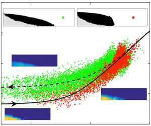
3.4. An effective $St$ definition: unifying closure models and laboratory experiments

Before discussing the rheological properties, we focus on the generalization of the above-mentioned results regarding the fluid phase closure models and with respect to experimental data available in the literature. So far, we have provided results for a given set of parameters of the closure models (2.6) and (2.8). According to the results discussed in the supplementary material, this specific set of parameters should contain all the required physics of the fluid phase at the microscale, smaller than $d$, to provide the expected behaviour of the collapse, at least qualitatively. This would mean that the influence of a specific choice of the closure model, in the range of that proposed in § 2.2, could only affect the dynamics quantitatively. We will show in this section that this quantitative influence of the closure models can actually be simply accounted for by defining an adequate effective Stokes number. Moreover, this will then be discussed in light of experimental results to highlight their predictability from the present simulations.

We have shown previously that the collapse is strongly affected by the transition from the viscous regime towards the free-fall regime. This transition has been shown to be controlled by the $St$ number according to many configurations involving fluid–particle interactions. One can thus anticipate that closure models, affecting viscous dissipation at the microscale, should modify the critical range of $St$ characterizing the transition from the viscous regime towards the free-fall regime. However, the qualitative trend obtained previously by varying $(St,\phi _i)$ should be maintained.

To highlight that assumption, different models have been considered for $\phi _i=0.63$ and varying $St$. The results are reported in figure 6(a). The different symbols correspond to different closure models, namely $(\xi =1, \eta _{eff}^M/\eta = 1+5\phi/2)$ (squares; circles correspond to the same closure models but with an extra lubrication force added into the DEM contact model as in Izard et al. (Reference Izard, Bonometti and Lacaze2014)), $(\xi =2,\eta _{eff}^M/\eta = 1+5\phi /2+7.6\phi ^2 + 16\phi ^3)$ (upward-pointing triangles), and $(\xi =3,\eta _{eff}^M/\eta = 1+5\phi /2+7.6\phi ^2 + 16\phi ^3)$ (downward-pointing triangles). One shows in this figure that providing a relevant definition of $St$, say $St^*$, allows the different cases almost to collapse onto a master curve. In particular, this modification of $St$ includes the influence of $\phi _i$ through the effective models as $St^*=St\times \eta /\eta _{eff}^M$ (open symbols in figure 6a) or $St^*=St/ ( \phi _i (1-\phi _i)^{-\xi } )$ (full symbols in figure 6a), i.e. accounting for the $\phi _i$ contribution included in either the effective viscosity closure model or the effective drag closure model, respectively. Note that, for the specific situation of an additional lubrication force in the contact model (circles), the definition of $St^*$ chosen as $St^*=St\eta /\eta _{eff}^M$ uses $\eta _{eff}^M/\eta = 1+5\phi /2+7.6\phi ^2 + 16\phi ^3$, even if the first-order Einstein viscosity was used here, as lubrication adds dissipation, which is not incorporated in the fluid phase solver. Then, one shows that models used for drag and/or viscosity, and even lubrication, only shift the transition from viscous to free-fall regimes, which could be easily understood using an appropriate definition of the $St$ number. This is a remarkable result, as it provides the relevance of the mesoscale approach for modelling immersed granular flows, even if the accurate closure models to be used are still debated.

Figure 6. (a) Ratio of the spreading length $L_f-L_i$ to the dry one $L_f^d-L_i$ as a function of the effective Stokes number $St^*=St\times \eta /\eta _{eff}^M$ (open symbols) or $St^*=St/ ( \phi _i (1-\phi _i)^{-\xi } )$ (full symbols) for the initially dense configuration $\phi _i=0.63$ (see text for details): simulations for $(\xi =1,\eta _{eff}^M/\eta = 1+5\phi /2)$ (squares) and an extra lubrication model (circles), $(\xi =2,\eta _{eff}^M/\eta = 1+5\phi /2+7.6\phi ^2 + 16\phi ^3)$ (upward-pointing triangle) and $(\xi =3,\eta _{eff}^M/\eta = 1+5\phi /2+7.6\phi ^2 + 16\phi ^3)$ (downward-pointing triangle); and experimental data from Bougouin & Lacaze (Reference Bougouin and Lacaze2018) (crosses with uncertainty). (b) Mean deposit slope $\tan {\alpha }$ as a function of $\phi _i$: numerical simulations for $(\xi =1,\eta _{eff}^M/\eta = 1+5\phi /2)$ and $St\approx 6\times 10^{-3}$ (black squares with uncertainty; blue squares correspond to the same simulations but shifting $\phi _i$ by $\approx 0.012$, a value based on the difference of rheological parameters between experiments and simulations, as explained in § 4.1), experimental data from Rondon et al. (Reference Rondon, Pouliquen and Aussillous2011) for $St\approx 5\times 10^{-2}$ (small dots) and for $St\approx 5\times 10^{-2}$ and $a\approx 0.5$ or $a\approx 0.65$ (big dots).

A comparison of the results with available experimental data is given in figure 6. More particularly, figure 6(a) compares the influence of $St$ in a dense configuration $\phi _i\approx 0.64$ on the spreading length as experimentally studied by Bougouin & Lacaze (Reference Bougouin and Lacaze2018), and figure 6(b) shows the comparison of the deposit angle as a function of $\phi _i$ at small $St$ as reported by Rondon et al. (Reference Rondon, Pouliquen and Aussillous2011). In figure 6(a), the final spreading length is shown relative to the dry one. This is done to ensure comparability between the numerical simulations and the experiments, for which the bottom surface is different. In figure 6(b), the comparison is done on the deposit slope $\tan {\alpha }$. Moreover, note that, here, the values of $St$ between numerical simulations and experiments are slightly different. However, their small values ensure a viscous regime, for which the final state remains roughly unchanged up to $St\approx 10^{-1}$. In both cases (figure 6a,b), a good agreement is obtained between the numerical simulations and the experimental data. In particular, the evolution of the final deposit as a function of $(St,\phi _i)$ is clearly captured and, moreover, the quantitative ranges of evolution are in reasonable agreement. Note that, as the value of $\phi _i$ is very sensitive, we also provide in figure 6(b) results for which $\phi _i$ is slightly shifted for the numerical data (blue squares; the shift value is not arbitrary and is based on the difference of equilibrium rheological states obtained in experiments and simulations as explained in § 4).

It can be noted that adding $\phi _i$ in $St^*$ only accounts for the rate of fluid dissipation induced by compaction in the granular pores. This allows one to capture the relevant range of variation of the final state as a function of fluid dissipation (figure 6a) but not to provide, solely, an explanation for the influence of $\phi _i$ at given $St$ reported in the previous section. In fact, the latter highlights a too significant influence on the final state to be attributed only to the definition of $St^*$. This shows again that the obtained results are to be linked to a significant influence of the rheological properties of the granular phase.

4.1. Influence of $St$ in the loose packing configuration

In this section, we focus on the initial loose packing configuration, i.e. $\phi _i=0.57$. This initial case is first considered as most of the initial column contributes to the granular motion, while for large $\phi _i$, most of the bottom-left corner remains static during the collapse. It will be shown that this configuration more clearly highlights an equilibrium state according to the rheological and state parameters $(\phi ,\mu )$, as obtained in steady flows.

The discussion on the rheological results obtained from the coarsening method is first discussed over the entire collapse without making any distinction between specific regions, i.e. over the domain $\mathcal {A}\in \{x > 2d, y > 2d, y < h(x,t)\}$, with $h$ the time-dependent height profile of the granular medium, and over a linear time-stepping scale, as $t\in [0, T_{95}]$ with a time step $T_{95}/10$. Note that $T_{95}$ is a function of $St$; thus this time stepping accounts for the different dynamics of the collapse to cover regularly the full range of evolution. Moreover, boundaries are excluded from the analysis, as they would need a specific attention such as an adapted coarse-graining approach (Weinhart et al. Reference Weinhart, Thornton, Luding and Bokhove2012).

Only the influence of $St$ is thus considered here. The results obtained from the coarse-graining approach are shown for $(St,\phi _i) = (6\times 10^{-3}, 0.57)$ (light green symbols) and $(St,\phi _i) = (6, 0.57)$ (dark green symbols) in figure 7. Note that larger values of $St$ have been performed up to $St=60$, for which no significant difference is observed from $St=6$. Thus $St=6$ is discussed here without altering the analysis. The volume fraction $\phi$ and the effective friction $\mu$ are plotted as functions of $K$ in figures 7(a) and 7(b), respectively. We can first note that, beyond an important dispersion of the results as anticipated, $\phi$ and $\mu$ show a clear evolution with respect to $K$, thus highlighting the relevance of the parameter $K$ as the controlling dimensionless parameter to describe the rheology of immersed granular material. Moreover, the two different cases $(St,\phi _i) = (6\times 10^{-3}, 0.57)$ and $(St,\phi _i) = (6, 0.57)$ nearly collapse onto a similar trend curve, even if a slight difference is actually observed, as will be discussed in the following. These observations reinforce the role of $K$, whose purpose is to unify the different regimes from viscous to free-fall.

Figure 7. (a) Volume fraction $\phi$ and (b) effective coefficient of friction $\mu$ as functions of $K$ for $(St,\phi _i)=(6\times 10^{-3},0.57)$ (light green dots) and $(St,\phi _i)=(6,0.57)$ (dark green dots). Inset: average data on a regular $K$ scale from rough local data. Solid lines correspond to model (4.3) with $\phi _c=0.592$, $a=0.18$, $\mu _c=0.24$, $\Delta \mu = 0.6$ and $\sqrt {K_0}=0.2$. Dashed lines correspond to the model used at large $St$ and extracted from figure 8(b), i.e. $\phi _c=0.6$ and $\mu _c=0.29$, keeping the other parameters equal to the former case.

The results obtained here show that, at small $\phi _i$, the rheology is not significantly affected by $St$, and that the obtained critical volume fraction $\phi _c=\phi (K\rightarrow 0)$ is larger than that in the initial state. These observations suggest that the rheological state is close to a somehow universal one, independent of the initial state, which should therefore be expected to be the one obtained for steady-state systems. We thus compare these results to the model proposed by Trulsson et al. (Reference Trulsson, Andreotti and Claudin2012) obtained for steady state and considered here as the equilibrium state rheology. This model can be written as

(4.3)\begin{equation} \left. \begin{gathered} \phi_{eq} =\phi_c - a\sqrt{K},\\ \mu_{eq} = \mu_c+\frac{\Delta \mu}{\sqrt{K_0/K}+1}, \end{gathered} \right\} \end{equation}

where subscript $eq$ stands for equilibrium. In figure 7, black solid lines correspond to the model (4.3) with $\phi _c=0.592$, $a=0.18$, $\mu _c=0.24$, $\Delta \mu = 0.6$ and $\sqrt {K_0}=0.2$. These values correspond to the best fit that can be obtained from the data shown in figure 7 for $St=6\times 10^{-3}$, which shows less dispersion. Moreover, the values for $\Delta \mu$ and $\sqrt {K_0}$ are consistent with results obtained for the dry collapse (Lacaze & Kerswell Reference Lacaze and Kerswell2009). This leads to values of the fitting data that are in reasonable agreement with what is obtained in the literature. It can also be noted at this point that the usual value of $\phi _c$ found in experiments is around $0.58$ (see, for instance, Pailha & Pouliquen Reference Pailha and Pouliquen2009). The $\approx 0.012$ difference of $\phi _c$ between experiments and simulations has thus been used as the shift value for $\phi _i$ in figure 6(b) (blue symbols).

The agreement between numerical results and the equilibrium model in figure 7 confirms the reliability of this model in the case of an unsteady and 3-D configuration for a large range of $St$, at least for $\phi _i=0.57$. However, a closer inspection of the results suggests that the influence of $St$ is not non-existent, and that the spatio-temporal domain of extraction of the rheological characteristics requires specific attention, as it highlights different states during collapse. This point is discussed in the following, and will also be considered attentively in the next section.

As mentioned above, the general rheological trend given in figure 7 is obtained at 10 regularly spaced time steps for $t\in [0, T_{95}]$. At large $St$, this includes both accelerating and decelerating stages of the collapse, while at small $St$ it only includes decelerating stages. This is highlighted in figure 8(a) in which the average value $\langle K\rangle$ is plotted as a function of $t/T_{95}$ for $St=6\times 10^{-3}$ and $St=6$, and with $\langle K\rangle$ being the spatial average of $K$ over the non-static area $\mathcal {A}_D\in \{x > 2d, y > h_s(x), y < h(x,t)\}$, where $h_s$ is the height profile delimiting the granular region which remains static for $t\in [0, T_{95}]$.

Figure 8. (a) Evolution of $\langle K\rangle$ as a function of time $t/T_{95}$ over the domain $\mathcal {A}_D$ (see text for details) for $(St,\phi _i)=(6\times 10^{-3},0.57)$ (black squares) and $(St,\phi _i)=(6,0.57)$ (grey squares). (b) Plot of $\mu _c$ (black squares) and $\phi _c$ (grey circles) as functions of $St$. Vertical lines in (b) indicate the typical uncertainty in evaluating $\mu _c$ and $\phi _c$.

We now focus on the decelerating stage, referred to as the resting stage, which is characterized as the time interval of decreasing $\langle K\rangle$. Note that, according to the results shown in figure 8(a), the case $St=6\times 10^{-3}$ is not significantly affected by this new procedure, as previous results were already obtained in the resting stage. However, this is somehow different for $St=6$, for which part of the coarse-grained results are removed with this new procedure. It explains the more important dispersion of results for $St=6$ in figure 7. Using this new procedure, each $St$ is investigated independently. The insets of figure 7 show the average values of $\phi$ and $\mu$, respectively, obtained on $\mathcal {A}_D$ during the resting stage, for the two values of $St$ considered previously. The average is obtained here by binning the spatio-temporal rough data in log-scale compartments of $K$. This first confirms the $K$ trend of both $\phi$ and $\mu$. Moreover, $\mu$ and $\phi$ merge at large $K$ for the different $St$, typically $K>10^{-3}$ here, i.e. at the beginning of the resting stage. This would naturally support the fact that the granular material has reached a universal equilibrium state. However, according to the definitions of $\phi _c$ and $\mu _c$ in (4.3) and obtained as $K\rightarrow 0$ during the resting stage, this refined investigation shows that they are both functions of $St$. The dependences of $\phi _c$ and $\mu _c$ with $St$ are shown in figure 8(b).

The evolution of $\mu _c(St)$ and $\phi _c(St)$ shown in figure 8(b) highlights a rapid transition around $St\approx 1$ delimiting two asymptotic behaviours at small $St$ and large $St$, at which plateaus are obtained. In particular, for both $\mu _c$ and $\phi _c$, the values on these plateaus are found to be slightly larger for $St\gg 1$ than for $St\ll 1$. Note that the value found at $St\gg 1$ is very close to that reported for dry collapses in Lacaze & Kerswell (Reference Lacaze and Kerswell2009). However, the physical reason for the sudden decrease of $\mu _c$ at small $St$ remains unclear, even if viscous/free-fall transitions are usual observations for several properties in different configurations (see, for instance, Gondret, Lance & Petit (Reference Gondret, Lance and Petit2002) for the case of particle bouncing). It can be at least noted that this is associated with the state of the granular medium for $K\rightarrow 0$, as $\phi _c$ follows a similar trend, such that $\mu _c$ decreases with $\phi _c$. This indicates an influence of the history of the collapse on the final state, through $St$, which leads to a small deviation from a universal equilibrium law.

For an unsteady configuration such as collapse, the state of the granular system and its associated rheological law, described here by $\phi$ and $\mu$ during the resting stage, i.e. for decreasing $K$, are close to the equilibrium law obtained for steady flows. However, the unique function of $K$ with constant parameters in (4.3) as obtained in steady configurations is not clear in the state. Here, different states can exist for the same value of $K$. In the loose configuration considered here, it has been shown to be possibly modelled by including a $St$ dependence in $\mu _c$ and $\phi _c$, keeping the trend of the equilibrium model. To finish with, note that the obtained evolution of $\mu _c(St)$ is in line with the conclusions drawn previously from the final state shape of the initial loose packing case, i.e. the spreading length increases while $\mu _c$ decreases for decreasing $St$ (see figure 5b).

4.2. Influence of $\phi _i$ at small $St$

The same procedure can be followed to identify the influence of the initial volume fraction $\phi _i$. As the influence of $\phi _i$ is clearer at small $St$, we focus here on $St=6\times 10^{-3}$. In this case, the granular flow remains in the viscous regime and then $K=J$. Figure 9 reports the coarse-graining results obtained over the temporal interval $t\in [0, T_{95}]$ with a time step $T_{95}/10$ and over the spatial domain $\mathcal {A}\in \{x > 2d, y > 2d, y < h(x,t)\}$, as done in the previous section. More particularly, the volume fraction $\phi$ and the effective coefficient of friction $\mu$ are plotted as functions of $J$ for $(St,\phi _i) = (6\times 10^{-3}, 0.57)$ (green symbols) and $(St,\phi _i) = (6\times 10^{-3}, 0.63)$ (blue symbols) in figures 9(a) and 9(b), respectively. Note, again, that the equilibrium law is recovered for $\phi _i=0.57$ on this spatio-temporal domain, as discussed in the previous section. Yet, as observed in figure 9, the case $\phi _i=0.63$ does not show the same trend as for $\phi _i=0.57$; the influence of the initial decompaction of the granular medium prior to collapsing cannot be disregarded from the rheological point of view. This behaviour has been reported in Pailha & Pouliquen (Reference Pailha and Pouliquen2009), specifying a dilatancy angle $\psi$ having to be accounted for when defining the effective friction angle. Following their analysis, we define the dilatancy angle $\psi$ as

(4.4)\begin{equation} \tan{\psi} = \boldsymbol{\nabla}\boldsymbol{\cdot} \langle \boldsymbol{v}\rangle_p. \end{equation}

Figure 9. (a) Volume fraction $\phi$ and (b) effective coefficient of friction $\mu$ as functions of $J$ for $(St,\phi _i)=(6\times 10^{-3},0.57)$ (green dots) and $(St,\phi _i)=(6\times 10^{-3},0.63)$ (blue dots). Inset of (a): Angle of dilatation $\tan {\psi }$ (4.4) as a function of $\phi$ for $(St,\phi _i)=(6\times 10^{-3},0.63)$. (c) Corrected coefficient of friction $\mu -\tan {\psi }$ as a function of $J$ (symbols are similar to panels a,b). Note that the dilatation effect for $\phi _i=0.57$ is hardly observable, so its correction $\tan {\psi }$ has therefore been neglected for this case (green dots in c); and the dilatation angle correction $\tan {\psi }$ is only observable when grain motion is significant enough, so data below $J\approx 10^{-4}$, i.e. in the plastic region, have therefore been disregarded for $\phi _i=0.63$ (blue dots in c). Solid lines in (a,c) correspond to model (4.5) with $\phi _{eq}=\phi _c$. Solid line in (b) corresponds to model (4.3).

The rheological model (4.3) can then be modified to include the influence of the dilatancy angle $\psi$ as discussed in Roux & Radjai (Reference Roux and Radjai1998) and Pailha & Pouliquen (Reference Pailha and Pouliquen2009),

(4.5)\begin{equation} \left. \begin{gathered} \tan{\psi}=b(\phi_{oeq}-\phi_{eq}),\\ \mu_{oeq} -\tan{\psi}= \mu_c+\frac{\Delta \mu}{\sqrt{K_0/J}+1}, \end{gathered} \right\} \end{equation}

where subscript $oeq$ stands for out of equilibrium. According to this model, $\mu -\tan {\psi }$ is plotted as a function of $J$ in figure 9(c), with the same symbols as previously. For $\phi =0.63$, only values above $J\approx 10^{-4}$ are reported here. As will be shown later, this is actually similar to considering only the moving region of the granular medium after the initial stages of the collapse corresponding to the initial expansion of the granular material. Below $J\approx 10^{-4}$, the $\mu -\tan {\psi }$ does not collapse on the same curve (not shown here). The reason can probably be attributed to the connection with the plastic region, which is not well captured by the $\mu (J)$ rheology (probably related to the behaviour of the $\mu (I)$ rheology at small $I$ as discussed in Barker & Gray (Reference Barker and Gray2017)). This very specific behaviour should be addressed in future works but is beyond the scope of the present paper, as it does not significantly affect the physics and the dynamics of the collapse. However, for $J> 10^{-4}$, one obtains a collapse of $\mu -\tan {\psi }$ onto a single function of $J$ for $\phi _i=0.57$ and $\phi =0.63$.

In order to predict simply the rheological behaviour shown in figure 9, we can first assume that $\phi _{eq}\approx \phi _c$ in (4.5), as it is shown to be roughly constant in the inset of figure 9(a) , where $\tan \psi$ is shown to be a single linear function of $\phi$ whatever $J$. This is, moreover, shown here to be equal to $\phi _c=0.592$ (intersection of the solid line and $\tan \psi =0$ in the inset of figure 9a ), similar to the value obtained with model (4.3) for $(St,\phi _i) = (6\times 10^{-3}, 0.57)$. The solid lines in figure 9(a,c) correspond to the model (4.5) with $\phi _{eq}=\phi _c$ keeping the values of $\mu _c$, $\Delta \mu$ and $K_0$ obtained previously and $b=5.5$. This model prescribes relatively well the trends of rheological parameters obtained from the simulations, particularly for $\mu -\tan {\psi }$ as a function of $J$ and $\tan \psi$ as a function of $\phi$, highlighting the influence of the deviation of the volume fraction $\phi$ with respect to a reference value $\phi _c$. Nevertheless, this model does not allow the trend of $\phi _{oeq}$ as a function of $J$ to be provided, i.e. model (4.5) is not closed as we basically end up with one equation for two unknowns $(\phi _{oeq},\mu _{oeq})$.

A slightly more advanced approach to close the rheological model (4.5) in our configuration would be to prescribe $\phi _{oeq}$. This is not necessarily an obvious task without solving an appropriate time-dependent equation. For the sake of simplicity, we propose in the following a prediction based on the expected behaviour of $\phi _{oeq}$, or more likely of $\tan \psi$, during the collapse. For that purpose, we rewrite the dilatancy angle $\psi$ such that

(4.6)\begin{equation} \tan \psi = -\frac{1}{\phi}\frac{\textrm{D}\phi}{\textrm{D}t}\dot{\gamma}^{-1} = -\frac{1}{\phi}\frac{\textrm{D}\phi}{\textrm{D}\tilde{t}}{J}^{-1}, \end{equation}

where $\tilde {t} = t/t_m$ with $t_m=\eta /\langle p\rangle _p$ is a microscopic time scale of rearrangement of the granular material in the viscous regime (Cassar et al. Reference Cassar, Nicolas and Pouliquen2005). As dilatation/compaction are precisely a rearrangement process, then we can assume that $({1}/{\phi }){\textrm {D}\phi }/{\textrm {D}\tilde {t}}= {O}(1)$ and then $\tan \psi \sim J^{-1}$. That said, we seek a solution that is also regular when $J\rightarrow 0$. As shown in figure 9(a), $\phi (J\rightarrow 0)$ can take several values. However, these values can be anticipated to be either $\phi _i$ or $\phi _c$, depending on the situation. These situations can be distinguished, as $J\rightarrow 0$ at two different stages of the collapse, say at the very beginning of the collapse and when reaching its final rest state. In particular, the former case $\phi (J\rightarrow 0)=\phi _i$ is more likely to be expected at the initial stage of the collapse, when the granular medium starts from an imposed volume fraction $\phi _i$. This will be referred to as the initiation stage. The latter case, $\phi (J\rightarrow 0)=\phi _c$, on the other hand, is more likely to be reached at the end of the collapse when the granular material returns to rest. As already discussed in the previous section, this resting stage could be considered as mainly described by its equilibrium state. This can be summarized as $\phi (J\rightarrow 0, t\rightarrow \{ 0;t_f\})=\{\phi _i;\phi _c\}$. A solution that would be consistent with (4.5) and (4.3) when $J\rightarrow 0$ should then have the form $\tan \psi \rightarrow b(\phi _i-\phi _c)$ for an initiation state and $\tan \psi \rightarrow b(\phi _c-\phi _c)=0$ for a resting state.

We thus propose the following simple model that would account for the out-of-equilibrium state during the granular collapse:

(4.7)\begin{equation} \left. \begin{gathered} \phi_{oeq} = \phi_{eq}+ \frac{ \left ( \{\phi_i;\phi_c\}- \phi_c \right ) {J}_1}{{J}+{J}_1} ,\\ \mu_{oeq}= \mu_{eq} + \frac{ b\left ( \{\phi_i;\phi_c\}- \phi_c \right ) {J}_1}{{J}+{J}_1}, \end{gathered} \right\} \end{equation}

where $\{\phi _i;\phi _c\}$ takes one of these values depending on the considered stage, i.e. initiation versus resting. Note, again, that, with this description, the resting stage is nothing but an equilibrium state. In (4.7) $J_1$ is a regularization term allowing one to reach a finite non-zero value when $J \rightarrow 0$. Its value is found here to be $J_1\approx 10^{-3}$ to fit the numerical data. This can be seen as the transition from the dominance of the dilatation/compaction effect towards a rheology controlled by the equilibrium state, this transition being found here to be controlled by the number $J$.

In order to show the relevance of the above-mentioned model, one proposes in the following to extract and to separate results from simulations during the so-called initiation stage and resting stage, labelled in the following as $(.i)$ and $(.ii)$, respectively. For that purpose, the distinction between these two stages has to be prescribed. We propose here to use the temporal evolution of averaged quantities over the granular medium. We thus plot the evolution of $\langle J\rangle$ and $\langle \phi \rangle$ as a function of $t/T_v$ in figure 10(a,b) for both $\phi _i=0.57$ (left column, labelled $L$ for loose) and $\phi _i=0.63$ (right column, labelled $D$ for dense). Recall that $T_v$ is a viscous time scale. Here, the procedure to obtain $\langle \cdot \rangle$ is the same as that explained in § 4.1 but over the domain $\mathcal {A}_{Dt}\in \{x > 2d, y > h_s(x,t), y < h(x,t)\}$, with $h_s$ delimiting the flowing region and plastic region at each time step. Note that domain $\mathcal {A}_{Dt}$ is slightly more restrictive than $\mathcal {A}_{D}$ as used previously in § 4.1.

Figure 10. Time-dependent rheology of the viscous collapse, $St=6\times 10^{-3}$, for $\phi _i=0.57$ (loose $L$, left column) and $\phi _i=0.63$ (dense $D$, right column). (a,b) Plots of $\langle J \rangle$ (black symbols) and $\langle \phi \rangle$ (grey symbols), averaged over domain $\mathcal {A}_{Dt}$ (see text for details), as a function of time (upper plots show snapshots of the granular medium within the different phases with static grains in grey and moving grains in black). (c,d) State and rheological parameters $\phi$ and $\mu$ as functions of $J$ for the different phases as labelled in each panel. In all panels, $(.0)$, $(.i)$ and $(.ii)$ correspond to the different stages of the granular flow according to its dynamical behaviour and rheological state: $(.0)$ is an initial decompaction stage prior to collapsing only observed for dense configuration $(D.)$; $(.i)$ corresponds to the initiation stage as an accelerating phase of the collapse; and $(.ii)$ is the resting stage during which the granular material goes to rest.

For the loose packing configuration $L$, one observes that the dynamics of the collapse, measured as $\langle J \rangle$, quickly reaches its maximum inertial state, and then $\langle J\rangle \rightarrow 0$. At the same time $\langle \phi \rangle$ increases during all the collapse (see figure 10a). However, in the log–linear representation of figure 10(a), the slope of $\langle \phi \rangle (t/T_v)$ suddenly changes. This also corresponds to a change in slope of $\langle J \rangle (t/T_v)$. This time is chosen as a delimitation of region $(L.i)$ and region $(L.ii)$. For the dense packing configuration, the evolutions of $\langle J \rangle$ and $\langle \phi \rangle$ are slightly different (see figure 10b). In particular, a first initial stage $(D.0)$ is observed during which $\langle J \rangle \approx 0$. This corresponds to the initial dilatancy during which both $\langle J \rangle$ and $\langle \phi \rangle$ evolve very slowly. Then $\langle J \rangle$ increases suddenly. The rest of the dynamics can also be separated into two stages $(D.i)$ and $(D.ii)$ roughly similarly to the loose configuration, and therefore corresponding to the initiation stage and resting stage. Here, however, the delimitation is characterized by an inversion of evolution of $\langle \phi \rangle (t/T_v)$ which decreases during $(D.i)$ and increases during $(D.ii)$. Note that, in both cases (loose and dense), the chosen delimitation between stages $(.i)$ and $(.ii)$ more clearly corresponds to a change in the evolution of the state of the granular medium through the evolution of $\langle \phi \rangle$. However, it is clear from figure 10(a,b) that this separation also delineates dynamical stages of the collapse, as for instance $\langle J \rangle$ is maximum during the initiation stage $(.i)$, while it slowly goes to zero during the resting stage $(.ii)$. On the other hand, stages $(.i)$ and $(.ii)$ actually correspond to significant difference in the mass evolution, and thus the run-out, between loose and dense configurations (as shown by the snapshot of the grains’ positions in figure 10a,b; black dots correspond to moving grains). In particular, $T_{95}$ is obtained at the end of stage $(L.ii)$ for the loose configuration, while it is at the end of $(D.i)$ or only early $(D.ii)$ for the dense one. Note that the latter observation explains the coarse-grained results shown in figure 9, as will be discussed later.

Using the above-mentioned delimitation in time, the rheological and state variables $\mu$ and $\phi$ are plotted as a function of $J$ during stage $(.i)$ (red dots) and stage $(.ii)$ (green dots) in figure 10(c,d). Here, coarse-graining is performed over the spatial domain $\mathcal {A}_{Dt}$. Even though coarse-grained results are a bit sparse, trends can be observed. These coarse-grained results are compared to the model (4.7) for $\phi (J\rightarrow 0, t\rightarrow 0)=\phi _i$ (solid line) and $\phi (J\rightarrow 0, t\rightarrow t_f)=\phi _c$ (dashed lines). The qualitative agreement between the model and the simulations confirms the assumptions used to obtain model (4.7).

To finish, we come back to the results obtained in figure 9. Recall that, there, coarse-grained results were obtained in the interval $t\in [0,T_{95}]$ over a regular time grid in a linear scale, and also includes the static region. According to results reported in figure 10 and the scale of $T_{95}$ for the loose and dense configurations, the spreading phase $t\in [0,T_{95}]$ mostly lasts at the end of $(L.i)$ and during $(L.ii)$ for the loose configuration, while it mostly lasts during $(D.i)$ for the dense one. In figure 11, one compares model (4.7) with this previously obtained coarse-grained results. The solutions of (4.7) are shown here for $\{\phi _i;\phi _c\}=\phi _i=[0.57:0.01:0.63]$ (thin lines), with highlights on $\{\phi _i;\phi _c\}=\phi _c$ (dashed line) and $\{\phi _i;\phi _c\}=\phi _i=0.63$ (solid line). We can first conclude that the model proposed is in good agreement with numerical data showing its relevance for out-of-equilibrium situations. Moreover, the dense packing configuration highlights more clearly an out-of-equilibrium law model with $\{\phi _i;\phi _c\}=\phi _i$ while the loose packing situation shows an equilibrium state, i.e. $\{\phi _i;\phi _c\}=\phi _c$, during most of the spreading phase $t\in [0, T_{95}]$. This latter remark does not mean that the loose configuration is not affected by the initiation stage, but that it happens on a short time scale compared to the entire collapse one, unlike the dense configuration.

Figure 11. Comparison of the coarse-graining results reported in figure 9 for $\phi _i=0.63$ (blue dots) and $\phi _i=0.57$ (green dots) with the model (4.7) (lines): (a) $\phi$ as a function of $J$ and (b) $\mu$ as a function of $J$. Dashed lines correspond to the equilibrium rheological model, i.e. $\phi _i=\phi _c$, while solid lines show the out-of-equilibrium model for $\phi _i=[0.57:0.01:0.63]$.